P Statistical Design and Analysis of Experiments
378
P Statistical Design and Analysis of Experiments Downloaded 12/11/12 to 129.128.207.242. Redistribution subject to SIAM license or copyright; see http://www.siam.org/journals/ojsa.php
Transcript of P Statistical Design and Analysis of Experiments

P Statistical Designand Analysis
of Experiments
Dow
nloa
ded
12/1
1/12
to 1
29.1
28.2
07.2
42. R
edis
trib
utio
n su
bjec
t to
SIA
M li
cens
e or
cop
yrig
ht; s
ee h
ttp://
ww
w.s
iam
.org
/jour
nals
/ojs
a.ph
p

P
9Statistical Design
and Analysisof Experiments
Peter W. M. JohnUniversity of Texas at Austin
Austin, Texas
51IITL.Society for Industrial and Applied Mathematics
Philadelphia
Dow
nloa
ded
12/1
1/12
to 1
29.1
28.2
07.2
42. R
edis
trib
utio
n su
bjec
t to
SIA
M li
cens
e or
cop
yrig
ht; s
ee h
ttp://
ww
w.s
iam
.org
/jour
nals
/ojs
a.ph
p
SIAM's Classics in Applied Mathematics series consists of books that were previouslyallowed to go out of print. These books are republished by SIAM as a professional servicebecause they continue to be important resources for mathematical scientists.
Editor-in-ChiefRobert E O'Malley, Jr., University of Washington
Editorial BoardRichard A. Brualdi, University of Wisconsin-MadisonHerbert B. Keller, California Institute of TechnologyAndrzej Z. Manitius, George Mason UniversityIngram Olkin, Stanford UniversityStanley Richardson, University of EdinburghFerdinand Verhuist, Mathematisch Instituut, University of Utrecht
Classics in Applied MathematicsC. C. Lin and L A. Segel, Mathematics Applied to Deterministic Problems in the Natura!Sciences
Johan G. F. Belinfante and Bernard Kolman, A Survey of Lie Groups and Lie Algebras withApplications and Computational Methods
James M. Ortega, Numerical Analysis: A Second Course
Anthony V. Fiacco and Garth P. McCormick, Nonlinear Programming: SequentialUnconstrained Minirnization Techniques
F. H. Clarke, Optimization and Nonsmooth Analysis
George F. Carrier and Carl E. Pearson, Ordinary Differential Equations
Leo Breiman, Probability
R. Bellman and G. M. Wing, An Introduction to Invariant Inbedding
Abraham Berman and Robert J. Plemmons, Nonnegative Matrices in theMathematica) Sciences
Olvi L Mangasarian, Nonlinear Programming*Carl Friedrich Gauss, Theory of the Combination of Observations Least Subject to Errors:Part One, Part Two, Supplement Translated by G. W. StewartRichard Bellman, Introduction to Matrix AnalysisU. M. Ascher, R. M. M. Mattheij, and R. D. Russell, Numerical Solution of Boundary ValueProblems for Ordinary Differential Equations
K. E. Brenan, S. L Campbell, and L. R. Petzold, Numerical Solution of Initial•Value Problemsin Differential Algebraic Equations
Charles L Lawson and Richard J. Hanson, Solving Least Squares Problems
J. E. Dennis, Jr. and Robert B. Schnabel, Numerical Methods for Unconstrained Optimizationand Nonlinear Equations
Richard E. Barlow and Frank Proschan, Mathematica) Theory of Reliability
Cornelius Lanczos, Linear Differential Operators
Richard Beliman, Introduction to Matrix Analysis, Second Edition
Beresford N. Parlett, The Symmetrie Eigenvalue Problem
Richard Haberman, Mathematical Models: Mechanica] Vibrations, Population Dynaniics, andTraffic Flow
Peter W. M. John, Statistica! Design and Analysis of Experiments
*First time in nrint.
Dow
nloa
ded
12/1
1/12
to 1
29.1
28.2
07.2
42. R
edis
trib
utio
n su
bjec
t to
SIA
M li
cens
e or
cop
yrig
ht; s
ee h
ttp://
ww
w.s
iam
.org
/jour
nals
/ojs
a.ph
p

Copyright © 1998 by the Society for Industrial and Applied Mathematics.
This SIAM edition is an unabridged republication of the work first published by TheMacmillan Company, New York, 1971.
10987654321
All rights reserved. Printed in the United States of America. No part of this book may bereproduced, stored, or transmitted in any maner without the written permission of thepublisher. For information, write the Society for Industrial and Applied Mathematics, 3600University City Science Center, Philadelphia, PA 19104.2688.
Library of Congress Cataloging-in-Publication Data
John, Peter William Meredith.Statistical design and analysis of experiments / Peter W.M. John.
p. cm. - (Classics in applied mathematics ; 22)"An unabridged republication of the work first published by the
Macmillan Company, New York, 1971 "--T.p. verso.Includes bibliographical references (p. - ) and index.ISBN 0-89871-427.3 (softcover)1. Experimental design. I. Title. II. Series.
QA279j65 1998 98-29392001.4'34-dc21
ELBJ1L is a registered trademark.
Dow
nloa
ded
12/1
1/12
to 1
29.1
28.2
07.2
42. R
edis
trib
utio
n su
bjec
t to
SIA
M li
cens
e or
cop
yrig
ht; s
ee h
ttp://
ww
w.s
iam
.org
/jour
nals
/ojs
a.ph
p

Contents
Preface xi
Preface to the Classics Edition
x111
References in the Preface xxiii
Chapter 1. Introduction
1.1 The Agricultural Heritage 21.2 An Example of an Experiment 31.3 Tests of Hypotheses and Confidence Intervals 51.4 Sample Size and Power 71.5 Blocking 81.6 Factorial Experiments 101.7 Latin Square Designs 121.8 Fractional Factorials and Confounding 121.9 Response Surfaces 141.10 Matrix Representation 14
Chapter 2. Linear Models and Quadratic Forms 17
2.1 Introduction 172.2 Linear Models 182.3 Distribution Assumptions 192.4 The Method of Least Squares 192.5 The Case of Full Rank 202.6 The Constant Term and Fitting Planes 212.7 The Singular Case 222.8 Pseudo-Inverses and the Normal Equations 232.9 Solving the Normal Equations 26
v
Dow
nloa
ded
12/1
1/12
to 1
29.1
28.2
07.2
42. R
edis
trib
utio
n su
bjec
t to
SIA
M li
cens
e or
cop
yrig
ht; s
ee h
ttp://
ww
w.s
iam
.org
/jour
nals
/ojs
a.ph
p
vi Contents
2.10 A Theorem in Linear Algebra 282.11 The Distribution of Quadratic Forms
29
2.12 The Gauss-Markoff Theorem
342.13 Testing Hypotheses 352.14 Missing Observations 37
Chapter 3. Experiments with a Single Factor 39
3.1 Analysis of the Completely Randomized Experiment
413.2 Tukey's Test for Treatment Differences
45
3.3 Scheffé's S Statistic
453.4 A Worked Example 463.5 Qualitative and Quantitative Factors and Orthogonal Contrasts 483.6 The Gasoline Experiment (Continued)
52
3.7 The Random Effects Model
523.8 The Power of the F Test with Random Effects 533.9 Confidence Intervaas for the Components of Variance 543.10 The Gasoline Experiment (Continued)
54
3.11 The Randomized Complete Block Experiment
553.12 The Gasoline Experiment (Continued)
58
3.13 Missing Plots in a Randomized Complete Block Design
593.14 The Analysis of Covariance
60
3.15 Analysis of Covariance for the Randomized Complete Block Design 63
Chapter 4. Experiments with Two Factors 66
4.1 The Two-Way Layout with One Observation per Cell 664.2 Orthogonality with More Than One Observation per Cell 684.3 The Two-Way Layout with Interaction 704.4 The Subdivision of the Sum of Squares for Interaction 734.5 Interaction with One Observation per Cell 754.6 The Random Effects Model 764.7 The Mixed Model 774.8 The Two-Stage Nested or Hierarchic Design 804.9 The Diallel Cross Experiment 81
Chapter 5. Experiments with Several Factors 86
5.1 Error Terms and Pooling 865.2 Replicates 875.3 The Complete Three-Factor Experiment 885.4 Approximate F Tests 92
Dow
nloa
ded
12/1
1/12
to 1
29.1
28.2
07.2
42. R
edis
trib
utio
n su
bjec
t to
SIA
M li
cens
e or
cop
yrig
ht; s
ee h
ttp://
ww
w.s
iam
.org
/jour
nals
/ojs
a.ph
p

Contents vii
5.5 An Experiment with Crossed and Nested Factors 945.6 General Rules for Sums of Squares and EMS 965.7 Split-Plot Designs 985.8 Split-Split-Plot Designs 1015.9 Computer Programs 102
Chapter 6. Latin Square Designs 105
6.1 Analysis 1066.2 Limitations of the Model 1086.3 Graeco-Latin Squares 1106.4 Sets of Orthogonal Latin Squares 1116.5 Experiments Involving Several Squares 1146.6 Change-Over Designs 1156.7 Change-Over Designs Balanced for Residual Effects 1176.8 Designs for Experiments with Residual Effects 120
Chapter 7. Factors with Two or Three Levels; Confounding 123
7.1 Factors at Two Levels 1247.2 Yates' Algorithm and the General 2n Design 1277.3 The 3'' Series of Factorials 1307.4 Confounding 1327.5 Partial Confounding 1347.6 Confounding 2n Designs in 2k Blocks of 2n - k Points Each 1367.7 The Allocation of Treatment Combinations to Blocks 1377.8 The Composition of the Defining-Contrast Subgroup 1397.9 Double Confounding and Quasi-Latin Squares 1407.10 Confounding in 3n Designs 1437.11 Confounding with Factors at More Than Three Levels 1447.12 Confounding in the 4 2 Design 1447.13 Confounding in Other Factorial Experiments 145
Chapter 8. Fractions of 2" Factorial Designs 148
8.1 The 2n - k Fractional Factorials 1498.2 The Classification of Fractions 1518.3 Some 2n - k Fractions 1528.4 Designs with Eight Points 1538.5 Designs with Sixteen Points 1558.6 Other 2n -k Fractions of Resolution V 1578.7 Blocking Fractional Factorials 158
Dow
nloa
ded
12/1
1/12
to 1
29.1
28.2
07.2
42. R
edis
trib
utio
n su
bjec
t to
SIA
M li
cens
e or
cop
yrig
ht; s
ee h
ttp://
ww
w.s
iam
.org
/jour
nals
/ojs
a.ph
p
viii Contents
8.8 Analyzing 2n - k Fractions8.9 Designs Obtained by Omitting 2n - k Fractions8.10 Three-Quarter Replicates8.11 The 3(25- 2) Designs8.12 Some 3(2n - k ) Designs of Resolution V8.13 Adding Fractions8.14 Nested Fractions8.15 Resolution III Designs8.16 Designs of Resolution IV
Chapter 9. Fractional Factorials with More Than Two Levels
9.1 3n Designs9.2 Latin Squares as Main Effects Plans9.3 3n - k Fractions with Interactions9.4 Orthogonal Main Effects Plans9.5 The Plackett and Burman Designs9.6 Addelman's Designs9.7 Fractions of 2m3n Designs of Resolution V9.8 Two Nonorthogonal Fractions of the 43 Design
Chapter 10. Response Surfaces
10.1 First-Order Designs10.2 Second-Order Designs10.3 3k Designs and Some Fractions10.4 Polygonal Designs for k = 210.5 Central Composite Designs10.6 Orthogonal Blocking10.7 Steepest Ascent and Canonical Equations10.8 The Method of Steepest Ascent10.9 The Canonical Form of the Equations10.10 Other Surfaces10.11 Evolutionary Operation10.12 The Method of Calculation
Chapter 11. Incomplete Block Designs
11.1 Balanced Incomplete Block Designs11.2 Some Balanced Incomplete Block Designs11.3 The Analysis of Balanced Incomplete Block Designs11.4 Resolvable Designs
159161163165167167170172173
177
178179181184185187190191
193
194196198201204206208209211213213216
219
220221223226
Dow
nloa
ded
12/1
1/12
to 1
29.1
28.2
07.2
42. R
edis
trib
utio
n su
bjec
t to
SIA
M li
cens
e or
cop
yrig
ht; s
ee h
ttp://
ww
w.s
iam
.org
/jour
nals
/ojs
a.ph
p

Contents ix
11.5 The General Incomplete Block Design 22711.6 The Adjusted Treatment and Block Totals 23011.7 Solving the Intrablock Equations 23011.8 Connected Designs 23311.9 The Recovery of Interblock Information 23311.10 Combining Intrablock and Interblock Estimates 23511.11 Some Computational Formulae for Combined Estimates 23811.12 Other Combined Estimates 24211.13 Maximum Likelihood Estimation 24211.14 The General Balanced Design 24511.15 Extended Incomplete Block Designs 248
Chapter 12. Partially Balanced Incomplete Block Designs 250
12.1 The Group Divisible Association Scheme 25212.2 Intrablock Analysis of GD Designs 25312.3 The Triangular Scheme 25412.4 The Latin Square Scheme (L £) 25512.5 The Cyclic Association Scheme 25512.6 The Intrablock Equations for PBIB(2) Designs 25612.7 Combined Intrablock and Interblock Estimates 25912.8 The Simple Lattice Design 26012.9 Partial Diallel Cross Experiments 26212.10 Choosing an Incomplete Block Design 265
Chapter. 13. The Existence and Construction of Balanced Incomplete BlockDesigns 268
13.1 The Orthogonal Series 27013.2 Series of Designs Based on Finite Geometries 27113.3 Designs Using Euclidean Geometries 27413.4 Designs Derived from Difference Sets 27513.5 Two Nonexistence Theorems 27613.6 The Fundamental Theorems of Bose 27713.7 Designs Derived from Symmetric Designs 28113.8 Designs with r < 10 28213.9 Series of Designs Based on Difference Sets 28313.10 Resolvable Designs 286
Chapter 14. The Existence and Construction of Partially Balanced Designs 288
14.1 Duality and Linked Block Designs 29014.2 The Elementary Designs 29114.3 Group Divisible Designs 292D
ownl
oade
d 12
/11/
12 to
129
.128
.207
.242
. Red
istr
ibut
ion
subj
ect t
o SI
AM
lice
nse
or c
opyr
ight
; see
http
://w
ww
.sia
m.o
rg/jo
urna
ls/o
jsa.
php
x Contents
14.4 Singular Designs 29314.5 Semiregular Designs 29314.6 Regular Designs 29514.7 Designs with the Triangular Scheme 30114.8 The Nonexistence of Some Triangular Designs 30514.9 Designs for the Latin Square Scheme 305
Chapter 15. Additional Topics in Partially Balanced Designs 310
15.1 Geometric Designs 31015.2 Latent Roots of the Intrablock and Interblock Matrices 31215.3 Cyclic Association Schemes 31515.4 Partially Balanced Association Schemes with Three Associate
Classes 31615.5 The Hierarchic Group Divisible Scheme 31715.6 The Rectangular Scheme 31815.7 The Cubic Scheme 31915.8 The Triangular Scheme for m = 3 32015.9 The LS3 Association Scheme 32115.10 Cyclic Designs 32215.11 Generalized Cyclic Designs 32415.12 Designs for Eight Treatments in Blocks of Three 32515.13 Conclusion 327
Appendix. Matrices and Quadratic Forms 329
A.1 Matrices 329A.2 Orthogonality 331A.3 Quadratic Forms 332A.4 Latent Roots and Latent Vectors 332A.5 Simultaneous Linear Equations 335
Bibliography 339
Index 351
Dow
nloa
ded
12/1
1/12
to 1
29.1
28.2
07.2
42. R
edis
trib
utio
n su
bjec
t to
SIA
M li
cens
e or
cop
yrig
ht; s
ee h
ttp://
ww
w.s
iam
.org
/jour
nals
/ojs
a.ph
p

Preface
This book, about the design of experiments, is for the mathematically orientedreader. It has grown primarily from courses that 1 have given during the pastdecade to first- and second-year graduate students in the statistics department atBerkeley and in the mathematics departments at the Davis campus of the Univer-sity of California and at the University of Texas.
My interest in experimental design began in 1957 when I became a researchstatistician for what is now Chevron Research Company (Standard Oil ofCalifornia). I had the particular good fortune to have the benefit of HenryScheffé as a consultant there, and subsequently as a colleague and friend. Thatwas the time when Scheffé's book on analysis of variance was just about to appear,when Box and Hunter were introducing the chemical engineers to responsesurface designs, and when engineers were becoming interested in 2n designs.At Davis 1 was able to teach a statistical methods course to graduate students inagricultural sciences, and at the same time 1 became interested in the combina-torial problems of the construction of incomplete block designs.
The book reflects all these phases. Although the treatment is essentiallymathematical, I have endeavored throughout to include enough examples fromboth engineering and agricultural experiments to give the reader the flavor of thepractical aspects of the subject.
The main mathematical prerequisite is a working knowledge of matrix algebraand an introductory mathematical statistics course. Unfortunately, courses onmatrices nowadays often seem to die before reaching quadratic forms, so 1 haveincluded an appendix dealing with them. There is no need for a knowledge ofmeasure theory, and the reader who is prepared to accept Cochran's theorem onfaith will need no calculus at all.
xi
Dow
nloa
ded
12/1
1/12
to 1
29.1
28.2
07.2
42. R
edis
trib
utio
n su
bjec
t to
SIA
M li
cens
e or
cop
yrig
ht; s
ee h
ttp://
ww
w.s
iam
.org
/jour
nals
/ojs
a.ph
p

xii Preface
From a practical standpoint, many readers will find the second chapter moredifficult than those that follow it. Unfortunately, this can hardly be avoided,whether one uses Cochran's theorem or Scheffé's geometric approach.
The choice of topics for a one-year course will vary with the interests of theinstructor and the mathematical abilities of the students. The first twelve chaptersare of interest to researchera and form the basis of a one-year course, with thechapter on Latin squares coming either at the end of the first semester or at thebeginning of the second. This allows the first semester to be devoted to analysis ofvariance and the complete factorial experiment. The second semester thencontains 2n and 3n designs, fractional factorials, response surfaces, and incompleteblock designs.
The last three chapters call for considerably more mathematical maturity thanthe others, and it is not necessary that the practitioner of experimental designread them. They take the reader to the frontier of research in the construction ofincomplete block designs, and a course for graduate students with a theoreticalemphasis should include some of these topics. Alternatively, I have sometimesused these chapters as the basis for an advanced seminar.
I am greatly indebted to my wife, Elizabeth, for her continued help andencouragement.
Austin, Texas P. W. M. J.
Dow
nloa
ded
12/1
1/12
to 1
29.1
28.2
07.2
42. R
edis
trib
utio
n su
bjec
t to
SIA
M li
cens
e or
cop
yrig
ht; s
ee h
ttp://
ww
w.s
iam
.org
/jour
nals
/ojs
a.ph
p

Preface to the ClassicsEdition
1. Introduction
In the 27 years since the initial publication of this book, much has changedin both application and theory of the design of experiments. The primecatalysts have been the personal computer (PC) and its increasingly sophis-ticated software, and the concomitant burgeoning of experimental designin industry. There are key debates over fixed, mixed, and random modelsin the analysis of variante and over the theory of optimal designs. Thissecond release gives me a welcome opportunity to comment about thesetopics and how they might have changed this book had it been writtentoday.
2. Computers
When I signed my contract with Macmillan in 1966, some, but by no meansall, statisticians had access to computers, which were big mainframes incomputer centers. One took one's problem to the center, together withthe necessary Fortran cards to suit the software package, and gave it to anemployee to have the data keypunched; the only package to which I cannow recall having ready access was the Biomed series. The whole thingwas handled through the bureaucracy of the computer center, who usuallycharged for their services. Some statisticians in industry had to send theirdata away to the computer at company headquarters. So most of us didwhat we ourselves could do on our desk calculators. Who of my generationdoes not recall the noise of the Friden desktop machine and such tricks asusing a machine with a large register so that one could accumulate x 2 onthe left, 2xy in the center, and y2 on the right?
Three decades later, we each have PCs of our own with (relatively) user-friendly software packages that will do, in a few seconds, analyses that used
xiii
Dow
nloa
ded
12/1
1/12
to 1
29.1
28.2
07.2
42. R
edis
trib
utio
n su
bjec
t to
SIA
M li
cens
e or
cop
yrig
ht; s
ee h
ttp://
ww
w.s
iam
.org
/jour
nals
/ojs
a.ph
p

xiv Preface to the Classics Edition
to take hours, and without the problems of making a charge to a budget.Not only can we do many things that we did not have the computer powerto do, we can do them while sitting at our own desks and at our own pace.I have not carried a job to the computer center in years. This has had anenormous influence on statistics in several ways. Obviously, we can performmore complex calculations than before and do our analyses more quickly,but there is more.
The "more" is manifested in a change of attitude. Graphics are so goodand so speedy that there is no excuse for a scientist not to plot his orher data and to spot obvious outliers or nonnormality. One can vet one'sdata as a matter of routine. More people can look at their own data andbecome interested in statistical analysis. They can display their analysesin presentations to colleagues in tables and charts. This can be a mixedblessing, however; someone who does not know what he or she is doing cando a lot of damage. Turning a graduate student loose on a data set armedwith a computer package and manual that are new to him or her (and withlittle knowledge of statistics) is a passport to disaster.
I will not take sides and recommend any particular computer package tothe reader, except to say that I use Minitab. I use Minitab for two reasons.The first is that I started my statistical computing with Minitab's father,Omnitab, many years ago, and I am too set in my ways to change, eventhough I do not question that there are other packages that may do somethings better. The second is that I find it a very easy package to use forroutine teaching purposes. It is very user friendly, and my students, someof whom are not strong on computer skills, can learn to do many standardthings very easily. The package does things at the click of a mouse thatI would never even have dreamed of attempting 30 years ago. I have nothad to take time to teach the abbreviated Doolittle method of invertingsymmetric matrices for so long that I have probably forgotten it.
One impact of the PC revolution is that, if this book were to be rewrit-ten, I would leave some sections out or radically alter them. I particularlyhave in mind Section 3.14 on analysis of covariance and Section 6.7 onchange-over designs with residual effects. The main thrust of these sectionswas to develop formulae to make the analysis systematic, and, therefore,relatively easy on a desk calculator. Today's reader does not need thoseformulae and should be spared the pain of reading about them. The miss-ing plot formulae of Section 3.13 and the first exercise in Chapter 6 areobsolescent, if not actually obsolete. Modern computer routines make thecalculations for such cases easy.
Readers whose interests in computing go beyond the scope of this bookmay be interested, for example, in such topics as programs to obtain solu-tions to the equations that arise when the method of maximum likelihoodis used to find estimates of components of variance. I shall mention laterthe use of computers to find D-optimal experimental designs.D
ownl
oade
d 12
/11/
12 to
129
.128
.207
.242
. Red
istr
ibut
ion
subj
ect t
o SI
AM
lice
nse
or c
opyr
ight
; see
http
://w
ww
.sia
m.o
rg/jo
urna
ls/o
jsa.
php

Preface to the Classics Edition xv
3. The growth of experimental design in in-dustry
In 1971, the vast majority of applications of analysis of variance and designof experiments were still in agriculture. There had been relatively little im-pact in industry in the United States and Europe outside Imperial ChemicalIndustries Ltd. in Great Britain, where George Box and his tolleagues didpioneering work, and in those oil and chemical companies whose membershad learned about 2n factorials and response surfaces from Box, often atGordon Research Conferences. Other engineers had little opportunity tolearn about that approach to experimentation. After all, Yates's (1937)monograph was published by the Imperial Bureau of Soil Science and dealtwith agricultural experiments, and there was little communication betweenaggies and engineers.
But in the 1980s, the growth of interest in experimental design acceler-ated as the emerging semiconductor industry became conscious of Japan'sindustrial success. Much of that success was attributed to the use of statis-tics that William Edwards Deming had advocated in Japan after WorldWar II and, in particular, to the resulting emphasis on designed exper-iments. The Japanese engineer, G. Taguchi, who had learned about 272
designs from Mahalanobis in India, introduced to the semiconductor in-dustry his methods for small complete factorials and orthogonal fractions.He was primarily concerned with main effects and paid little attention tosuch complications as interactions. Taguchi's method reduces design ofexperiments to a relatively simple drill, to which some companies requirestrict adherence. That has some merit, as long as it works, but it does notlead to a very deep understanding. However, Taguchi went further. Hemade us think not just about experiments to find conditions that optimizeyield, but also about experiments to control the variability of a manufac-turing process.
At about the same time, the advent of the PC made the requisite calcu-lations much easier. We no longer had to use Yates's algorithm to analyze2n factorials. It became easier to analyze them, or their fractions, by re-gression, especially since the I.C.I. group had persuaded us to think of thelevels of the factors as —1, +1 instead of 0, 1, as Yates had used. Run-ning nonorthogonal fractions was no longer so daunting because we couldactually analyze the data when it came in! The journal Techinometrics,which had first appeared in 1959 and to which there are numerous refer-ences in the 1971 edition of this book, thrived, publishing numerous paperson design of experiments.
Engineers came to realize that they no longer had to associate de-signed experiments solely with the large complete factorial experiments,planted in the spring and gathered in the fall, that were the tradition ofDow
nloa
ded
12/1
1/12
to 1
29.1
28.2
07.2
42. R
edis
trib
utio
n su
bjec
t to
SIA
M li
cens
e or
cop
yrig
ht; s
ee h
ttp://
ww
w.s
iam
.org
/jour
nals
/ojs
a.ph
p

xvi Preface to the Classics Edition
the agronomists. They could think of series of small experiments: runningan exploratory fractional experiment and then, after seeing the results,running further points to answer the questions that the analysis of the firstexperiment raised.
Performing a set of small experiments in sequence quite logically leadsone to consider running the points of an individual experiment in a plannedsequence. Often they will be run one after another anyway, which itselfimplies a sequence. Why not arrange the order so that the estimates of theeffects will be orthogonal to time trends? Cox (1951) was the first to writeabout this. Hill (1960), Daniel and Wilcoxon (1966), Steinberg (1988),and John (1990) all wrote about the topic in Technometrics. Dickinson(1974) wrote about sequences from another point of view: How can weorder the points so as to minimize the cost of all the changes in factorlevels that a factorial experiment requires? Another relevant question ishow to order the points so that early termination will still leave us with aviable, though incomplete, set of data? (Section 8.14 touches upon the lastof these questions.)
4. Fixed, mixed, and random models
In 1971, the question of the expected values of the mean squares in theanalysis of factorial experiments seemed to have been settled by Scheffé(1956). In Section 4.7, I gave an account of Scheffé's method of analyzingthe two-factor experiment in which one factor, A, is fixed and the other,B, is random. One tests the mean square for A against the mean squarefor interaction; on the other hand, one tests the mean square for B againstthe mean square for error. An essential feature of Scheffé's model is that,since A is fixed, we should impose the side condition > (a/3)jj = 0 for eachj. In deriving E(SB) we can argue that we sum (average) the interactionsover all the levels of the fixed factor A; hence, they "cancel out," and nointeraction term appears in E(SB).
Hocking (1973) introduced an alternative model in which the interac-tions were freed of those side conditions. In Hocking's model the interactionterm appears in both E(SA) and E(SB), and so MA and MB are each testedagainst MAB. Scheffé's model has come to be called the restricted modeland Hocking's the unrestricted model. Practitioners are given a difficultchoice. Bach model has a logical basis, and the differences are subtle; eachmodel can be defended and each has its advocates. I had no difficulty in1971. Hocking had not yet written his paper. The only approach of whichI was aware was Scheffé's, and so that was the only one that I described.
In Section 5.3 I gave a set of rules for computing the expected values ofthe mean squares (EMS) in a crossed classification for three factors (usingScheffé's model). One writes down the EMS as if all three factors wereD
ownl
oade
d 12
/11/
12 to
129
.128
.207
.242
. Red
istr
ibut
ion
subj
ect t
o SI
AM
lice
nse
or c
opyr
ight
; see
http
://w
ww
.sia
m.o
rg/jo
urna
ls/o
jsa.
php

Preface to the Classics Edition xvii
random, and then one strikes out certain interaction terms that involvefixed effects, following rule 4. The reader should now call this rule 4r (tocorrespond to the restricted rule) and add the following rule 4u (if he orshe wishes to use the unrestricted rule).
4.1. Rule 4u
In the unrestricted rule, an interaction is called fixed if and only if all itsfactors are fixed. Otherwise, it is random. In the expected mean squarefor any effect, strike out any interaction that is fixed and leave the others.Do not strike out an interaction from its own EMS.
In the case of three factors with A random and B and C fixed, the onlyfixed interaction is BC. We strike it out of the expectations of the meansquares for B and C, but we do not strike it out in the line for BC itself.Because A is random, we do not strike out the ABC interaction from anymean square.
The restricted rule is much more liberal than the unrestricted rule instriking out terms.
These distinctions also apply to the general balanced design in whichsome factors are crossed and others are nested. We can still begin byfollowing the first four steps of the procedure of Bennett and Franklin thatis described in Section 5.6.
Step 5 should be revised as follows.
Write the EMS, assuming that all the factors are random and followingthe rules that (i) each line of the EMS table contains all the terms that haveas subscripts all the letters in the title of the line, and (ii) the coefficient ofany component is the product of the levels of all the factors that correspondto absent subscripts. Then strike out terms using step 5r or step 5u.
4.2. Step 5r (the restricted rule)
If some of the factors are fixed, we strike out of the expectation of anymean square all those terms that contain in their live subscripts any letters(other than those in the name of the mean square itself) that correspondto fixed effects.
4.3. Step 5u (the unrestricted rule)
We strike out an interaction term only if all its live subscripts belong tofixed effects.Dow
nloa
ded
12/1
1/12
to 1
29.1
28.2
07.2
42. R
edis
trib
utio
n su
bjec
t to
SIA
M li
cens
e or
cop
yrig
ht; s
ee h
ttp://
ww
w.s
iam
.org
/jour
nals
/ojs
a.ph
p
xviii Preface to the Classics Edition
5. Optimal designs
Kiefer (1959) presented to the Royal Statistical Society a paper about hiswork on the theory of optimal designs. How do we choose between onedesign for p factors in n points and another? How do we find the best de-sign? This book mentions the criterion of minimizing the average varianceof the estimates of the effects, which came to be known as A-optimality ortrace-optimality.
Kiefer spoke of D-optimality, choosing the design that maximized thedeterminant, D, of X'X, where X is the design matrix. How does one findsuch a design?
The factors can be discrete or continuous. Users of 2n factorials havethe discrete case with xi = ±1. Mitchell (1974) published his DETMAXalgorithm, enabling us to find a design that maximizes D when the exper-imental space has a finite number of points. His algorithm has since beenimproved and is now available in some standard software packages, so thatan engineer has only to type in the values of n and p and the model (withor without interactions), and out comes a design.
It is all very easy, but there are questions in addition to the obviouspossibility of local maxima. The criterion is very sensitive to the model.Suppose that the model has q terms. If you drop one of the terms, adesign that was optimal for q terms in n runs is not necessarily optimal forq — 1 terms in n runs, nor does an optimal design for q factors in n pointsnecessarily contain a subset that is a D-optimal design for n — 1 points.
Also, the solution in any case may not be unique. If one permutes thecolumns of X, or if one multiplies any column by minus one, which corre-sponds to changing the level of that factor at every point, D is unchanged.One can call such solutions isomorphic to one another. But there are non-isomorphic solutions in some cases. In the small problem of fitting maineffects and two-factor interactions for a 2 4 factorial in 12 points, there are4 families of nonisomorphic solutions, all with the same maximum value ofD, and one of them is a foldover design! Furthermore, none of them is anoptimal plan for main effects only. In this case, an optimal design is givenby any 4 columns of the Plackett and Burman design for 11 factors in 12runs.
The continuous case is beyond the scope of this book. Its mathematicaldemands go further into measure theory and functional analysis than mostof our readers wish. It has become a flourishing field of research among themore mathematically oriented statisticians. A survey of the field written byAtkinson (1982) has more than 100 references, including books by Fedorov(1972) and Silvey (1980). A follow-up survey by the same author in 1988has many more.D
ownl
oade
d 12
/11/
12 to
129
.128
.207
.242
. Red
istr
ibut
ion
subj
ect t
o SI
AM
lice
nse
or c
opyr
ight
; see
http
://w
ww
.sia
m.o
rg/jo
urna
ls/o
jsa.
php

Preface to the Classics Edition xix
6. Incomplete block designs
I have written of some areas that have grown in interest since 1971. Sadly,I must comment on an area which has quietly disappeared from the radarscreen of experimental design: incomplete block designs. In 1971, it was animportant topic, and it still provides opportunity for some interesting andelegant mathematics. I have enjoyed working on some of its problems overthe years, but I must confess that it is an obsolescent topic, a victim to theadvance of computers. I contributed a paper to the 1982 commemorativevolume for Yates about running 2'factorials in incomplete block designs,and published a follow-up paper in 1984, but applications of the resultsseem to have been few and far between, if, indeed, there have been any!
7. Finis
By contemporary standards, mine has been an unusual career. Nowadaysyoungsters are expecteded to set a straight path almost as soon as theybecome upper-division undergraduates and pursue it doggedly to the end.My path has zigged and zagged with the help of some outstanding teachersto whom I am deeply grateful. I began as a pure mathematician and firstencountered statistics in 1948 in the postgraduate diploma (now M.Sc.)course at Oxford, where I was taught by David Finney, P.A.P. Moran, andMichael Sampford. Upon coming to the United States, I set statistics asidefor a few years while earning a Ph.D. in probability.
Then an extraordinary opportunity occurred in industry. In 1957 Ijoined Chevron Research Corporation in Richmond, California, as theirfirst statistician. In effect, that gave me a 4-year postdoctoral period work-ing with Henry Scheffé, whom Chevron had retained as its consultant inthe previous year. Chevron sent me to Gordon Conferences on Statistics,which were then dominated by George Box and his pioneering work in theapplication of design of experiments to chemical engineering and, in par-ticular, to response surfaces. The conferences had an electric atmosphereof intellectual ferment. At the same time, Henry set me to read the Box—Wilson (1951) paper and the I.C.I. book on industrial experimentation,edited by my fellow Welshman Owen Davies. I learned a lot from thatbook. The level of exposition is excellent and, unlike the spring of 1949,when Sampford was lecturing about design to a young mathematician whohad never seen a real experiment, I now knew what an experiment was.Real ones were going on all around me.
After 4 invaluable years at Chevron, I chose to return to the academieworld, where I have been ever since. I greatly enjoy teaching. Indeed, atHenry's instance, for the last 3 of those years I had taught a course in thestatistics department at the University of California, Berkeley, in additionDow
nloa
ded
12/1
1/12
to 1
29.1
28.2
07.2
42. R
edis
trib
utio
n su
bjec
t to
SIA
M li
cens
e or
cop
yrig
ht; s
ee h
ttp://
ww
w.s
iam
.org
/jour
nals
/ojs
a.ph
p

xx Preface to the Classics Edition
to my work at Chevron. Now I also wanted the freedom to work on anyproblem that attracted me, regardless of its importante to the company.An ideal opportunity beckoned from the mathematics department at theUniversity of California, Davis, one of the world's foremost agriculturalresearch domains. This involved me in a remarkable new array of exper-iments, including the large factorials of the agronomists with their fixed,mixed, and random models. Finally, in 1967, I moved to a large mathe-matics department at the University of Texas, which has no tradition ofresponsibility for any statistical services to the campus community.
This book, begun in Davis, was largely written in the relative isolationof Austin, where I have remained for personal reasons. Happily, continuinginvolvement in the Gordon Conferences and consulting kept me in touchwith real-world stimuli until another remarkable opportunity emerged fromthe new semiconductor industry.
In cooperation with the federal government, a consortium of companiesin that industry established in Austin a research facility called SematechCorporation. For several years I have been fortunate to work with membersof their statistical methods group. My collaboration with them has led towork in such areas as nonorthogonal fractions, D-optimal designs, andmultivariate analysis of variance. I have learned that engineers do indeedcarry out large factorial experiments with crossed and nested factors andmixed models; they call them gauge studies!
My path has zigged and zagged but, in retrospect, each turn ultimatelyafforded stimulating new experiences and opportunity for growth. Morethan ever, I share Henry Scheffé's (1958) conviction that industry is avaluable source of research problems. The first question that he was askedas a consultant for Chevron led him to invent a new branch of experimentaldesign: experiments with mixtures. He told me repeatedly that there aredozens of interesting problems out there in industry, just below the surface,waiting to be solved, if only one is alert enough to spot them and run withthem. That brings me to the role of serendipity and the thesis that a lotof useful research comes from a combination of luck, accident, and beingin the right place at the right time.
This is true of two problems, to which I have referred above, from mydays at Chevron. The idea of running the points of a factorial experimentin a prescribed sequence so as to protect against early termination cameErom an accident. A client wanted to do a 2 factorial on a pilot plant whichhe had at his disposal for 2 weeks, enough to do one complete replicate.I knew the "correct" thing to do. We carefully listed the 16 points andarranged them in random order. Fate struck. After 8 points, the pumpquit, and could not be repaired within the 2-week period. Have you everseen an experiment that consists of 8 points chosen at random from all16? It is a mess. With the benefit of hindsight, we realized that it wouldhave been a lot smarter if, instead of randomizing the 16 points, we hadD
ownl
oade
d 12
/11/
12 to
129
.128
.207
.242
. Red
istr
ibut
ion
subj
ect t
o SI
AM
lice
nse
or c
opyr
ight
; see
http
://w
ww
.sia
m.o
rg/jo
urna
ls/o
jsa.
php
Preface to the Classics Edition xxi
arranged for the first eight points to be either a resolution IV half replicatedefined by I = +ABCD, or I = —ABCD, in random order. Then wewould have had a design with good salvage value when the darned pumpbroke. Clearly, it would have been better to modify the randomization.
The other example led to my interest in nonorthogonal fractions. I hadpersuaded an engineer to try a 2 factorial. The raw material came from afacility in Scotland by slow boat. They sent enough for only 6 runs. I knewwhat to do with 8 runs; I knew what to do with 4 runs; but 6 was betwixtand between. I had to work out what to do. That led me to 4 factors in12 runs, and thus to three-quarter replicates.
Both problems arose by accident. They should never have happened.A referee of a paper about one of them objected that the problem wascontrived. It certainly was not. It was a real-life situation that probablywould not have occurred to me had I just spent my time in an ivory-toweroffice thinking about mathematical theorems in the design of experiments.
Henry Scheffé was right. There are all kinds of practical research prob-lems lurking in industrial applications, just waiting to be found and solved.I advise students to keep their eyes open and spot them. Some can betremendously interesting and full of theoretical challenge. Above all, beinghelpful to people is rewarding in itself.
I end with the sentence that concluded my original preface. It is stilltrue. I am greatly indebted to my wife, Elizabeth, for her continued helpand encouragement.
Austin, Texas P. W. M. J.
Dow
nloa
ded
12/1
1/12
to 1
29.1
28.2
07.2
42. R
edis
trib
utio
n su
bjec
t to
SIA
M li
cens
e or
cop
yrig
ht; s
ee h
ttp://
ww
w.s
iam
.org
/jour
nals
/ojs
a.ph
p

References in the Preface
ATKINSON, A. C. (1982). "Developments in Design of Experiments." Int. Statist.Rev., 50, 161-177.
ATKINSON, A. C. (1988). "Recent Developments in the Methods of Optimumand Related Experimental Designs." Int. Statist. Rev., 56, 99-116.
Box, G. E. P., AND K. J. WILSON (1951). "On the Experimental Attainmentof Optimum Conditions." J. Roy. Statist. Soc. Ser. B., 13, 1-45.
Cox, D. R. (1951). "Some Systematic Experimental Designs." Biometrika, 38,312-323.
DANIEL, C., AND F. WILCOXON (1966). "Factorial 2P -9 Designs Robust AgainstLinear and Quadratic Trends." Technometrics, 8, 259-278.
DAVIES, O. L. (1954). Design and Analysis of Industrial Experiments. Oliver andBoyd, London.
DICKINSON, A. W. (1974). "Some Run Orders Requiring a Minimum Number ofFactor Level Changes for the 2 4 and 2 Main Effect Plans." Technometrics,16, 31-37.
FEDOROV, V. (1970). Theory of Optimal Experiments. Academic Press, NewYork.
HILL, H. H. (1960). "Experimental Designs to Adjust for Time Trends." Tech-nometrics, 2, 67-82.
HOCKING, R. R. (1973). "A Discussion of the Two-way Mixed Model." Amer.Statist., 27, 148-152.
JOHN, P. W. M. (1982). "Incomplete Block designs for the 2 Factorial." UtilitasMath., 21, 179-199.
JOHN, P. W. M. (1984). "Incomplete Block Designs for the 24 Factorial." UtilitasMath., 26, 79-88.
JOHN, P. W. M. (1990). "Time Trends and Factorial Experiments." Technomet-rics, 31, 275-282.
KIEFER, J. (1959). "Optimal Experimental Designs (with discussion)." J. Roy.Statist. Soc. Ser. B, 21, 272-319.
MITCHELL, T. J. (1974). "An Algorithm for the Construction of `D-Optimal"Experimental Designs." Technometrics, 16, 203-210.
xxiii
Dow
nloa
ded
12/1
1/12
to 1
29.1
28.2
07.2
42. R
edis
trib
utio
n su
bjec
t to
SIA
M li
cens
e or
cop
yrig
ht; s
ee h
ttp://
ww
w.s
iam
.org
/jour
nals
/ojs
a.ph
p

xxiv
References in the Preface
SCHEFFÉ, H. (1956). "A Mixed Model for the Analysis of Variance." Ann. Math.Statist., 27, 23-36.
SCHEFFÉ, H. (1956). "Alternative Models for the Analysis of Variance." Ann.Math. Statist., 27, 251-271.
SCHEFFÉ, H. (1958). "Experiments with Mixtures." J. Roy. Statist. Soc. Ser. B,20,344-360.
SCHEFFÉ, H. (1959). The Analysis of Variance. John Wiley and Sons, New York.
SILVEY, S. D. (1980). Optimal Design. Chapman—Hall, London.
STEINBERG, D. (1988). "Factorial Experiments with Time Trends." Technomet-rics, 30, 259-270.
YATES, F. (1937). The Design and Analysis of Factorial Experiments. ImperialBureau of Soil Science, Harpenden, England.
Dow
nloa
ded
12/1
1/12
to 1
29.1
28.2
07.2
42. R
edis
trib
utio
n su
bjec
t to
SIA
M li
cens
e or
cop
yrig
ht; s
ee h
ttp://
ww
w.s
iam
.org
/jour
nals
/ojs
a.ph
p

CHAPTER 1
Introduction
It is the view of many statisticians, amongst whom the author counts himself,that statistics is a branch of applied mathematics, and that its health and growthdepend upon the involvement of the statistician in practical problems. This bookdeals with one of the interfaces between applied mathematics and scientificinvestigation: the design of experiments.
To some scientists, the idea that a statistician can contribute substantially tothe design of an experiment is, if not patently absurd, at least dubious. A commonimage of statisticians is one of people who are rather clever with figures and henceuseful for reducing data to tables; the statistician might be of some help in theanalysis, but only if there are reams of data to feed into computers. One hopes thatthis false image is fading with the passage of time. Meanwhile, however, thisattitude frustrates the statistician and deprives the scientist of valuable help.
It is true that the statistician is not usually an expert in the particular areas ofbiology or engineering in which the experiments are being made. It is true alsothat, given a computer, or for that matter enough time, pencils, and paper, one canfit a straight line or a plane to almost any hodgepodge of data whether relevant ornot. The bigger the computer, the more variables it can handle in a multipleregression program, and, unfortunately, the more miles of useless numbers it canprint out. It is clear, therefore, that some planning before the data is obtained is inorder, and that the planning had best be made with the method of analysis of theexperiment as well as its objectives in mind.
It follows that the role of the statistician in an experimental program should benot merely to analyze the results of the experiment, but also to help the scientistplan his experiment in such a way as to produce valid results as efficiently aspossible. There is little sense in waiting until the end of the experiment and then
Dow
nloa
ded
12/1
1/12
to 1
29.1
28.2
07.2
42. R
edis
trib
utio
n su
bjec
t to
SIA
M li
cens
e or
cop
yrig
ht; s
ee h
ttp://
ww
w.s
iam
.org
/jour
nals
/ojs
a.ph
p

2 Introduction [Ch. 1
visiting the statistician for the first time with a pile of data to deal with as best hecan. Every applied statistician can tell horror stories of having been asked afterthe event to analyze data from lengthy and expensive experiments which were sobadly planned that no valid conclusions could be drawn from them. There arealso numerous experiments which, although valid results have been obtained,would have yielded even more information if skilled knowledge of design hadfigured in the planning, and others in which the results obtained could, withefficient design, have been obtained with less effort and expense.
This book is written for the mathematically oriented statistician, scientist, andengineer. The basis of all the theory of design and analysis will be the linear modeland the analysis of variance, and throughout we shall refer the reader to the bookby Henry Scheffé (1959). It is the most authoritative book available on theanalysis of variance and is invaluable as a reference book. The examples that weinclude are drawn from various fields; most of them are taken from the publishedliterature, and some of them come from experiments in which the author hasparticipated as a consultant.
1.1 The Agricultural Heritage
The pioneer in the use of mathematical statistics in the design of experimentswas the late Sir Ronald Fisher. He dominated the bistory of experimental designbetween the First and Second World Wars, 1918-1939. During the early partof that era he was in charge of statistics at the Rothamsted Agricultural Experi-ment Station near London. In 1933 he succeeded Karl Pearson as GaltonProfessor at the University of London and later he moved to a professorship atCambridge University. It was Fisher who introduced the analysis of variance.He wrote two books about experimental design, each of which has run intoseveral editions, even though neither is by any means easy to read: StatisticalMet hods for Research Workers, which first appeared in 1925, and The Design ofExperiments. Dr. F. Yates joined Fisher at Rothamsted in 1931, and throughoutthis book the reader will find references to the major contributions of Yates andhis colleagues at the agricultural experiment station.
From this background it has naturally followed that the common terminologyof experimental design comes from agriculture, where they sow varieties in orapply treatments to plots and often have the plots arranged in blocks. We shalluse this terminology except when we think in terms of engineering applications,and then we shall talk about points or runs. The terms point and run will beused interchangeably; we make a run on the plant at a predetermined set ofconditions, and the result will be an observation or a data point (pedants wouldsay datum point). It sometimes puts engineers off to hear a statistician talkabout plots when he discusces their experiments. Some engineers tend to jumpto the superficial conclusion that the statistician is locked into a rigid frameworkof agricultural thinking and hence can contribute little to the solution ofengineering problems.
Dow
nloa
ded
12/1
1/12
to 1
29.1
28.2
07.2
42. R
edis
trib
utio
n su
bjec
t to
SIA
M li
cens
e or
cop
yrig
ht; s
ee h
ttp://
ww
w.s
iam
.org
/jour
nals
/ojs
a.ph
p

Sec. 1.2] An Example of an Experiment 3
This ignores the essential fact that the statistician really thinks in terms oflinear mathematical models. He is distinguished from many experimenters, whoare deeply involved in their own specialized sphere, by mathematical trainingwith a certain amount of emphasis on abstract thinking. This makel it easierfor him to see the essential mathematical similarity between an experimentcomparing varieties of barley and an experiment comparing operating tem-peratures in a catalytic cracker at an oil refinery.
The process of designing an industrial experiment is not, however, just amatter of taking a standard design from an agricultural handbook and substi-tuting temperature for variety and run for plot. Indeed, differences do existbetween agricultural and industrial experimentation, and, with all the incumbentrisks of generalizing, we suggest a few. One is that the agronomist usually has tosow his experimental plots in the spring and harvest them in the fall. Plots andplants are relatively cheap, and the emphasis has to be on. designing relativelycomplete experiments; if anything is omitted it will have to wait until next year.On the other hand, much industrial experimentation can be carried out relativelyquickly, in a matter of days rather than months, but experimental runs areoften very expensive. The emphasis should, therefore, be on small experimentscarried out in sequence, with continual feedback of information, so that indesigning each stage the experimenter can make use of the results of the previousexperiments.
The agronomist is more interested in the tests of significance in the analysisof variance than is the industrial experimenter. One of the reasons is that theagronomist is more often concerned with uniformity trials. Can he producestrains of seed that are essentially equivalent? Can he produce a new variety ofseed that will do well, not just on the experimental farm at Davis, California,but all up and down the hot Central Valley and perhaps also in the coastalregion, in the other states where the erop is grown, and even in other countries?He wants to be able to accept the null hypothesis of uniformity. The positionof the industrial experimenter often differs from that of the agronomist in twoways: he frequently knows before starting the experiment that his treatmentsare not all the same and is interested in finding out which ones differ and byhow much. His emphasis will be on estimation rather than hypothesis testing.He will sometimes argue that failure to reject the null hypothesis is merely theresult of taking too small an experiment. Expecting to reject the null hypothesis,he is more interested in confidence intervals.
In the sections that follow we shall introduce the topics of the various chaptersby considering a typical experiment.
1.2 An Example of an Experiment
Suppose that a chemical engineer hopes to improve the yield of some petro-chemical in an oil refinery plant by comparing several catalysts. Crude oil is fedinto the plant, which is charged with the catalyst; some of the crude oil, or
Dow
nloa
ded
12/1
1/12
to 1
29.1
28.2
07.2
42. R
edis
trib
utio
n su
bjec
t to
SIA
M li
cens
e or
cop
yrig
ht; s
ee h
ttp://
ww
w.s
iam
.org
/jour
nals
/ojs
a.ph
p

4 Introduction Ch. 1]
feedstock, passes through the plant unchanged; some is converted into thepetrochemical, or product. The liquid that comes out of the plant is separatedinto product and unconverted feedstock, and the yield, or response, is thepercentage of feedstock converted into product.
An obvious procedure is to make one or more plant runs using each of thecatalysts and to compare the average yields on each catalyst. There are, how-ever, some other considerations that enter the picture. How many catalysts?How many runs? How do we compare these averages after we have obtainedthem? Let us assume for the moment that the crude supply is plentiful andconsider just two catalysts, A and B, which make up the simplest situation.We take r runs on each catalyst, N = 2r runs altogether, and we obtain averageyields yl on A and y2 on B.
The first of our mathematica) models now enters the picture. Let y ij denotethe yield on the jth run made with the ith catalyst; y ij is a random variable andwe assume y t; = m i + eij where m i is the true value for the ith catalyst and e^ 5 isa random component of error or noise. We further assume that on the averagethe noise contribution is zero; sometimes it is positive and sometimes negative,but it averages out over the long haul, in the sense that E(e 5) = 0, and soE(y11) = m ; . Then yt will be an unbiased estimate of m i , and yl — y2 will be anunbiased estimate of m l — m 2 .
The word random should not be passed over lightly. The use of randomizationis the keystone of the application of statistical theory to the design of experi-ments, and the validity of our deductions rests upon the principle of randomiza-tion. The very least that can be said as a recommendation for randomization isthat it is only prudent to avoid the introduction of systematic bias into anexperiment. An agronomist comparing two varieties of corn would not rationallyassign to one variety all the plots that were in the shade and to the other all theplots that were in the sun. If he did, he would not be able to teil after the experi-ment whether any apparent difference in yields resulted from varietal differencesor from the fact that one variety had more sun. Furthermore, Fisher (1947) hasshown that the fact that the treatments have been randomly assigned to the runsis itself an adequate basis for obtaining tests of significance and confidenceintervals.
The other maxim of experimental design emphasized by Fisher was replicationto provide a proper estimate of the error variance, V(et;). If we were to taker = 1 and obtain y l = 80, Y2 = 79, we should not be able to make conclusionsabout the relative potencies of the catalysts with much confidence. We could pickthe winner and recommend catalyst A because y l l > y21, but we should have noidea whether the apparent difference was genuine or a result of noise (error). Ifwe made several runs with each catalyst, and found that the observations werehighly repeatable, i.e., that the range of the observations on A, and the range ofthe observations on B were both very small, we could be happy about concludingthat m l > m 2 when we observed yl > y2 . On the other hand, if the observationson both A and B were scattered between 60 and 90, a difference between themeans of only one would hardly be convincing.
Dow
nloa
ded
12/1
1/12
to 1
29.1
28.2
07.2
42. R
edis
trib
utio
n su
bjec
t to
SIA
M li
cens
e or
cop
yrig
ht; s
ee h
ttp://
ww
w.s
iam
.org
/jour
nals
/ojs
a.ph
p

Sec. 1.3] Tests of Hypotheses and Confidence Intervals 5
1.3 Tests of Hypotheses and Confidence Intervals
Deciding whether or not an observed difference between the sample meansyl and y2 is convincing evidence of a real difference between m l and m 2 isequivalent to testing the hypothesis Ho : m l = m2 . There is no need for us to gointo the details of the Neyman—Pearson theory of hypothesis testing at thistime, or to discuss the merits of one-tailed or two-tailed tests. The reader will befamiliar with these topics already. Nor is this the place to rekindle the Hames ofcontroversy between the confidence intervals that we shall employ and fiducialintervals; it suffices to say that in practice the intervals are the same and theargument is of little import.
It is at this stage of the proceedings that we have to make some decisions aboutwhat we shall assume to be the nature of the random errors e t; . We mentionthree possibilities:
(i) We could assume only that the treatments were assigned to the runs, orthe plots, by some process of randomization. This would lead us to theconsideration of randomization models and permutation tests. We shallnot take this road because not very much has been done with thisapproach for designs other than randomized complete blocks and Latinsquares. The reader may wish to refer to the discussions of the randomiza-tion models and tests given by Kempthorne (1952) and (1955), Scheffé(1959), Wilk and Kempthorne (1955) and (1957). Nor shall we considerthe nonparametric rank order tests of the Wilcoxon type.
(ii) We could assume that the errors are (a) uncorrelated random variableswith zero expectations and the same variance o 2 , or else (b) randomvariables with zero means and a covariance matrix that is of known form.
(iii) We could add to assumption (ii) the additional assumption of normality.
For obtaining our estimates under assumption (ii), we shall rely upon themethod of least squares. For testing hypotheses we shall make the normalityassumption and use F tests and t tests.
Returning to our earlier model under assumptions (iia) and (iii), we now haveyi; = m t + et; where the errors e i; are independent normal random variables,each with mean zero and variance o 2 . The least squares estimates m t of theparameters m i are obtained by minimizing the sum of squares of the residuals,
se = (Yii — mt) 2 ^t i
and they are, as we suspected all the time, m t = ƒi . We can also obtain an esti-mate of a 2 by comparing repeated observations on the same treatment. Lookingfirst at A, J; (y, ; — y^) 2 is an unbiased estimate of (r — 1)u 2 . If there are ttreatments, E(Se) = t(r — 1)a2.
Dow
nloa
ded
12/1
1/12
to 1
29.1
28.2
07.2
42. R
edis
trib
utio
n su
bjec
t to
SIA
M li
cens
e or
cop
yrig
ht; s
ee h
ttp://
ww
w.s
iam
.org
/jour
nals
/ojs
a.ph
p

6 Introduction [Ch. 1
When two treatments are to be compared, the statistic z = (j — y2)/^/(2Q2/r)has a normal distribution with mean m 1 — m2 and variance unity, which weshall write as z — N(m 1 — m2 , 1). If Q2 is not known, we shall substitute for Cr 2
the estimate s2 = SQ/(rt — t). The resulting statistic, when m l = m2, hasStudent's t distribution with t(r — 1) degrees of freedom.
No great difficulties are introduced if the numbers of observations are notthe same for each treatment. Suppose that there are r ; observations on theith catalyst. As before, m ; = y; , and now
E (Se) = E{^ (j)t1 — yt) 2} _ (rt — 1)a2 = (N — t)°2,
where N = ^, r1 . The estimate of a2 is thus 52 = Se/(N — t). When the hth andith treatments are to be compared, the statistic
_ Yn — Yt_ t s(1/rh + 1/ri) 1I2
has, if mh = m i , Student's distribution with (N — t) degrees of freedom.There is, however, a problem if the variance of ejj changes from treatment
to treatment. Consider again two treatments and suppose that the variancesof the random variables involved are V(e11) = a and V(e21) = 02. Then, ifthere are r{ observations on the ith treatment,
V (Yl — Y2) = r1 lal + r2 1az = v2 ,
and (y1 — Y2) — N(m l — m2i v2).If cri and oZ are known, v2 is easily computed, and the distribution of
(Yl — Y2)/v is standard normal. If, however, neither oi nor a2 is known, the bestestimates of them from the data are s; = (y — y1)2 /(r, — 1).
We let w; = rti 's?. Unfortunately, the random variable t' _ (yl — Y2)/(w1 + w2)"2 does not have the Student's distribution and its distribution has tobe approximated. There are several approximations that can be used, and wemention two of them. The disparity between the distributions of t and t' is leastwhen r1 = r2 .
Cochran and Cox (1957, page 101) give a procedure for obtaining an approxi-mation to the critical value of t' for any level a. Let 0 { = rt — 1. Then thecritical value is t* = (wl tl + w2 t2)/(w l + w2), where ti is the critical value, atthe desired level a, of Student's t with 0 t degrees of freedom.
Welch (1947) approximates the distribution of t' by a Student's t distributionwith 0 d.f., where
0 = 919'2(wl + W2)2/(ç61w1 + 2w2)•
The assumption of equal variances is usually not unreasonable, especiallywhen two similar treatments are being compared. Scheffé (1959) devotes a
Dow
nloa
ded
12/1
1/12
to 1
29.1
28.2
07.2
42. R
edis
trib
utio
n su
bjec
t to
SIA
M li
cens
e or
cop
yrig
ht; s
ee h
ttp://
ww
w.s
iam
.org
/jour
nals
/ojs
a.ph
p
Sec. 1.4] Sample Size and Power 7
chapter to the consequences, in the analysis of variance, of departures fromassumptions (ii) and (iii). In some cases where the variance is believed to dependupon E(y) in a known manner, the variance can be stabilized bytransformingthe data. These transformations do not necessarily eliminate the nonnormality,but they leem to alleviate it somewhat.
If V(y) = {g(y)} 2, and if z is a single-valued function of y, the variance of z isapproximated by
vz = (azl a ) 2 V(y).
If v is to be a constant, we therefore need to have
z = c f [g(Y)] -1 dY,
where c is an arbitrary constant. If g(y) is directly proportional to y, the trans-formation z = In y is appropriate; in y denotes the natural logarithm of y;logla y will do just as well. For binomial data the transformation z = Arcsin ymay be used, but this is often not done if the range of y is not large, especiallywhen p is about 0.5. When p = 0.5 we have pq = 0.25, and when p = 0.3 orp = 0.7 the product pq only decreases to 0.21.
1.4 Sample Size and Power
If the experimenter has at his disposal a prior estimate of the variance o 2, heis in a position to make some approximate power calculations. Most readers willalready be acquainted with the procedures for computing r in the case of onlytwo treatments, when type I and II errors are given. If the experimenter hasdecided to use a one-sided normai test with type I error a to compare twomeans, he will reject the hypothesis Ho : m l = m2 in favor of the alternativeHA : m l > m2 if yl — y2 > c. The cutof point c is given by c = zaa /(2/r) whereZa is the upper a point of the standard normal density, i.e., P(z > za) = a.
Suppose now that he wants to choose r to be so large that if m l = m2 + Sohe will have probability t1 — P) of deciding that m l > m2, i.e., of havingyl — Y2 fall in the critical region. He must then have
P(Y1 —y2 <c^m l —m2 =8a)=P.
It follows that
SQ — c = zsu/(2/r) and 8 = (za + zs)V(2/r).
This gives an approximate value
r=2(za+zs)2/S-2
Dow
nloa
ded
12/1
1/12
to 1
29.1
28.2
07.2
42. R
edis
trib
utio
n su
bjec
t to
SIA
M li
cens
e or
cop
yrig
ht; s
ee h
ttp://
ww
w.s
iam
.org
/jour
nals
/ojs
a.ph
p

8 Introduction [Ch. 1
In practice, however, the sample size is often determined not by calculationsof power but by real or imagined considerations of the budget. If a prior estimateof the variance is available, a variation of the previous calculation is still worthcarrying out. To revert to our earlier example, suppose that previous experiencein the plant gives a prior estimate az = 2 and that the engineer wishes to detectthat the new catalyst A is better than the old catalyst B if m l — m2 >_ 2 =but that he is only prepared to make n = 4 runs with each of the catalysts. Letus suppose further that he wishes to use a = 0.05. We have z a = 1.645, 6 = ^/2.
Then zs = 0.355 and P = 0.36, so that there is about one chance in three thatwith n = 4 he will fail to reveal an actual improvement of 2 units with hisexperiment. If 6 had been one, corresponding to m l — m2 >_ 1.4, the chance ofdetection would have been only about four in ten (0.4). This kind of information,even if it is a rough approximation, is salutary to the engineer. It should at leastserve to make his hopes for the outcome of his experiment more realistic. It mayeven prompt him to abandon or to revamp completely an investigation that wasdoomed to be unproductive.
When there are several treatments, similar calculations can be made involvingthe power of the Ftest. This is discussed by Scheffé (1959), Graybill (1961), andKempthorne (1952). Scheffé uses the charts by Pearson and Hartley (1951) andby Fox (1956). The other two books contain Tang's tables based upon theincomplete Beta distribution.
1.5 Blocking
There are two ways in which we can reduce the variance of m l — m2 . Wecan take more data points, i.e., increase r and thereby increase the cost of theexperiment, or we can somehow improve the design.
Some reduction can be made by refinement in experimental technique and byimproved methods of measurement and chemical analysis, but these improve-ments are limited in their achievement and there still remains what might becalled the natural noire of the system. Some engineers have difficulty acceptingthe fact that a system or a procedure has a built-in variability. This is true foranalytical procedures, and the American Society for Testing Materials has triedhard to make its members realize that in standard measurements a certain amountof variability is to be expected because of the nature of the measurementprocedure. Hence, failure to have duplicate measurements identical is notnecessarily an indication of incompetence on the part of the operator. It isregrettable that in some laboratories duplicate measurements are uselessbecause the atmosphere is such that the operator feels so strong a pressure tohave his second reading conform to the first reading that the second readingcan by no stretch of the imagination be considered as an independent observa-tion. W. J. Youden has suggested that second readings obtained in this wayshould be regarded not so much as duplicate readings as duplicity; they certainly
Dow
nloa
ded
12/1
1/12
to 1
29.1
28.2
07.2
42. R
edis
trib
utio
n su
bjec
t to
SIA
M li
cens
e or
cop
yrig
ht; s
ee h
ttp://
ww
w.s
iam
.org
/jour
nals
/ojs
a.ph
p
Sec. 1.5] Blocking 9
give the scientist a false sense of confidence in his results. Genuine duplicates canbe obtained by sending the analytic laboratory coded samples, e.g., pouring agallon of product into eight pint bottles and calling for a single determinationon each of the eight "different" samples. It is a nuisance to have to do this, butit is often worth the trouble, and the results can be quite revealing.
One way of improving the precision of estimates of differences, such asm l — m2i is by blocking. If there are t catalysts, perhaps we can take a barrel ofcrude oil, divide it into t parts, and use one part with each catalyst. The agricul-tural equivalent is to divide a field into blocks and then to subdivide each blockinto t plots. This topic is discussed at the end of Chapter 3. When we have acompletely randomized design in which the runs are made in completelyrandom order, or in which the plots with any given treatment are scattered allover the field, then comparisons between treatments contain additional vari-ability from the fact that some runs are made from one barrel and some fromanother, or that some are made on good land and some on stony land. The ideabehind the blocking is that by balancing the treatments over the blocks we makethe differences between the blocks cancel out when we compare the treatments.The individual estimates of m l and m2 are no better than they were before, in thesense that V(y) has not been reduced, but V(yl — y2) has hopefully suffered aconsiderable reduction.
This is the randomized (complete) block experiment, and the reader shouldnote that the word randomized appears again. We assign the treatments atrandom to the runs within each block; we should perhaps be suspicious if wealways used the first sample drawn from each barrel for catalyst A and the lastsample for catalyst B that there might be some systematic bias introduced. Wemodify our earlier model and, letting yl; denote the observation on the ithtreatment in the jth block, we write ytf = m ; + b1 + e{; where b; is the effect ofthe jth block. We shall actually write the model a little differently later when wecome to look at it a little more closely.
This procedure works well so long as each barrel of crude oil is big enoughto handle t runs, and the randomized complete block design is said to be themost commonly used experimental design. If, however, the blocks are not bigenough to accommodate all the treatments, we have to resort to incompleteblocks, with k (<t) treatments being contained in each block. The topic ofincomplete block designs is introduced in Chapter 11. If we cannot arrange tohave every pair of treatments appear together in every block, perhaps we canarrange the design so that every pair appears in A blocks where t is a constant.Such a design is called a balanced incomplete block design. These designs wereintroduced by Yates in 1936, but long before then such arrangements of symbolshad been of interest to pure mathematicians. Number theorists have for yearsinvestigated the combinatorial properties of these designs without any care forpossible statistical applications. Chapter 13 is devoted to the problems of theconstruction of balanced incomplete block designs. It is a chapter for mathe-maticians, and the experimenter who simply wants a particular design for hisexperiment might be content to look it up in the Fisher and Yates tables.
Dow
nloa
ded
12/1
1/12
to 1
29.1
28.2
07.2
42. R
edis
trib
utio
n su
bjec
t to
SIA
M li
cens
e or
cop
yrig
ht; s
ee h
ttp://
ww
w.s
iam
.org
/jour
nals
/ojs
a.ph
p

10 Introduction [Ch. 1
The restriction that each pair of treatments shall appear in exactly A blocks isdemanding, and designs do not exist for all values of t, k, and A. In 1939 Boseand Nair introduced partially balanced incomplete block designs. These designsare the topics of Chapters 12 and 14, the latter chapter being devoted to theconstruction of the designs for different partially balanced schemes. In partiallybalanced designs each treatment appears with n l of the other treatments ,1 1 times,with n 2 of them d2 times, and so on. There are also some further restrictions, butthey can wait until Chapter 12.
Just as one would not normally use an incomplete block design when asuitable complete block design is available, so balanced incomplete blockdesigns are preferable to partially balanced designs because of their higherefficiency. The measure of efficiency is the average of the variances of theestimates m,, — m i for all pairs of treatments; the measure is made scale free bydividing it by the average that would be obtained for a complete block designwith the same number of observations, if such a design could have been used.Kempthorne (1956a) conjectured, and J. Roy (1958) proved that for any givenset of numbers N, t, k (k < t) the most efficient incomplete block design is thebalanced design; that is, if one exists.
1.6 Factorial Experiments
We have just talked about blocking as a technique for improving the precisionof the estimates (mh — m i). The block effects b. canceled out of the comparisonbetween the treatments. We were thinking at thé time of the block differences asa nuisance to be eliminated. The idea was to avoid the differences between thecrude oils by balancing them out over the treatments. We could, however,purposely choose one barrel of Venezuelan crude oil, one of Sumatran, one ofCalifornian, one of Texan, and so on. This would give us two factors: catalystsand types of oil. The structure is very similar to that of the blocked experiment.Just as each catalyst "sees" each barrel of oil, so each type of oil "sees" eachcatalyst. The crude oil differences cancel out of comparisons between catalysts;the catalyst differences cancel out of the comparisons between crude oils.
We can rewrite our model to take into account two factors, A and B, the latterstanding either for blocks or for another factor:
yti; =m+ai +b5 +ejj .
Here m is a grand mean effect, a, is the main effect of the ith level of A, and bj isthe main effect of the jth level of *B. We talk of the several crude oils as beinglevels of the factor "crude oil." The terminology sounds artificial in this context,but its justification becomes more apparent when we think of a quantitativefactor such as temperature at levels of 100, 200, and 300 degrees.
The model that we have just written is an additive model. It may beinadequate. It could happen that the first catalyst is clearly better than the
Dow
nloa
ded
12/1
1/12
to 1
29.1
28.2
07.2
42. R
edis
trib
utio
n su
bjec
t to
SIA
M li
cens
e or
cop
yrig
ht; s
ee h
ttp://
ww
w.s
iam
.org
/jour
nals
/ojs
a.ph
p

Sec. 1.6] Factorial Experiments 11
others on all crude oils except the Sumatran, which might perhaps have a highersulfur content. This failure of the additive model, inasmuch as the expectationof the difference between observations on different crude oils does not remainconstant from catalyst to catalyst, is an example of interaction between thefactors. Interaction is an added complication, and at this stage the experimenterhas to face up to a problem that he should have thought about earlier. Fromwhat populations did the levels of the factors that were used come? If thecatalysts are some specific types having perhaps an alumina base, a silica base,and so on, we have a fixed factor, meaning that the levels are fixed effects, andthe parameters a i are unknown constants. The objective would then be toinvestigate comparisons between the parameters a i .
On the other hand, suppose that the barrels of crude oil were all drawn fromday-to-day production in the same California oil field. The effect b. would be arandom variable representing the day-to-day variation in the quality of the oil.Then B would be a random factor, and the objective would usually be to obtainan estimate of the component of variance V(b) = ob.
If both factors are fixed, we have a fixed effects model. If both are random, wehave a random effects model. If there is one of each, we have a mixed model.The analysis, particularly in regard to the choice of denominators for the Fstatistics, depends upon which of these three types of model is relevant. This isdiscussed for the case of two factors in Chapter 4.
In Chapter 5 we turn to factorial experiments with several factors. Some ofthe further development is a routine extension of the results of Chapter 4 to afew more dimensions. There are, however, other complications and variationsthat will be considered at that time. One of them merits mention now.
Let us return for a moment to the crude oils and the catalysts. Suppose thatthere is indeed within each oilfield barrel-to-barrel variation in the quality of thecrude oil, and that we take three barrels from each of four fields and make onerun with each catalyst from each of the twelve barrels. This is an example ofwhat is called a split plot experiment. The catalysts see every barrel, and sobarrel differences cancel out in comparing catalysts. However, in comparingcrude oils each crude oil average contains the variability only of its own barrels,and this does not cancel out.
The term split plot comes from the agricultural background at Rothamsted.A modern example of split plots occurs with the use of crop-dusting aircraft.One possibility is to take several fields; these will be the plots, or the whole plots.We now divide the field into strips and plant each strip with a single variety ofbarley; if there are enough strips we may have several strips to each variety.These strips are the subplots. Suppose now that we also want to test somefertilizers. We can then fertilize each complete field with the same fertilizer byspraying it from an aircraft. Comparisons between fertilizers will be madebetween whole fields. Comparisons between varieties of barley will be madebetween strips in the same field. Conversely, one could apply the differentfertilizers by hand to the different strips in the fields, and then sow the seeds afield at a time from an aircraft. A more complicated approach would be to sow
Dow
nloa
ded
12/1
1/12
to 1
29.1
28.2
07.2
42. R
edis
trib
utio
n su
bjec
t to
SIA
M li
cens
e or
cop
yrig
ht; s
ee h
ttp://
ww
w.s
iam
.org
/jour
nals
/ojs
a.ph
p
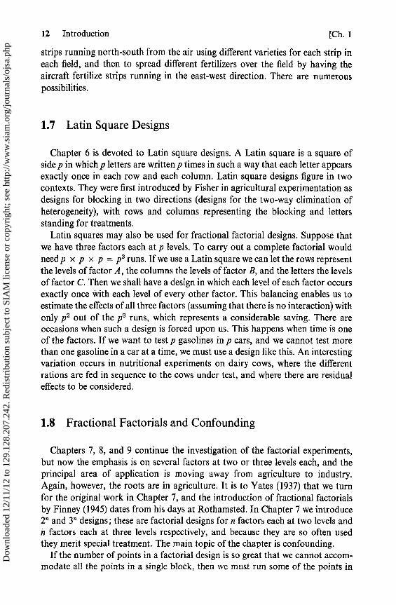
12 Introduction [Ch. 1
strips running north-south from the air using different varieties for each strip ineach field, and then to spread different fertilizers over the field by having theaircraft fertilize strips running in the east-west direction. There are numerouspossibilities.
1.7 Latin Square Designs
Chapter 6 is devoted to Latin square designs. A Latin square is a square ofside p in which p letters are written p times in such a way that each letter appearsexactly once in each row and each column. Latin square designs figure in twocontexts. They were first introduced by Fisher in agricultural experimentation asdesigns for blocking in two directions (designs for the two-way elimination ofheterogeneity), with rows and columns representing the blocking and lettersstanding for treatments.
Latin squares may also be used for fractional factorial designs. Suppose thatwe have three factors each at p levels. To carry out a complete factorial wouldneedp x p x p = p 3 runs. If we use a Latin square we can let the rows representthe levels of factor A, the columns the levels of factor B, and the letters the levelsof factor C. Then we shall have a design in which each level of each factor occursexactly once with each level of every other factor. This balancing enables us toestimate the effects of all three factors (assuming that there is no interaction) withonly p2 out of the p3 runs, which represents a considerable saving. There areoccasions when such a design is forced upon us. This happens when time is oneof the factors. If we want to test p gasolines in p cars, and we cannot test morethan one gasoline in a car at a time, we must use a design like this. An interestingvariation occurs in nutritional experiments on dairy cows, where the differentrations are fed in sequence to the cows under test, and where there are residualeffects to be considered.
1.8 Fractional Factorials and Confounding
Chapters 7, 8, and 9 continue the investigation of the factorial experiments,but now the emphasis is on several factors at two or three levels each, and theprincipal area of application is moving away from agriculture to industry.Again, however, the roots are in agriculture. It is to Yates (1937) that we turnfor the original work in Chapter 7, and the introduction of fractional factorialsby Finney (1945) dates from his days at Rothamsted. In Chapter 7 we introduce2n and Y' designs; these are factorial designs for n factors each at two levels andn factors each at three levels respectively, and because they are so often usedthey merit special treatment. The main topic of the chapter is confounding.
If the number of points in a factorial design is so great that we cannot accom-modate all the points in a single block, then we must run some of the points in
Dow
nloa
ded
12/1
1/12
to 1
29.1
28.2
07.2
42. R
edis
trib
utio
n su
bjec
t to
SIA
M li
cens
e or
cop
yrig
ht; s
ee h
ttp://
ww
w.s
iam
.org
/jour
nals
/ojs
a.ph
p

Sec. 1.8] Fractional Factorials and Confounding 13
one block, and the remainder in one or more other blocks. One of the possiblecontrasts between the data points will coincide with the differente between theblock totals. That degree of freedom is said to be confounded with blocks.Clearly we should not like, for example, to include all the points at high tempera-ture in one block and all the points at low temperature in the other block,because then the temperature effect, if any, would be hopelessly confused orconfounded with the block effects. We should like to divide the design intoblocks in such a way that the division does as little damage as possible to thedesign.
In Chapters 8 and 9 we turn to fractionation. We have already mentioned theLatin square design as a 1/3 fraction of a factorial with three factors, each atthree levels. There are several reasons for the extensive use of fractional fac-torials. The relatively high cost of industrial experimentation makel it essentialthat the designs used be as economical and as efficient as possible. Runs on arefinery unit may cost several thousand dollars a time, and, even though theeventual payoff may be many times more than that, management decisionmakers are usually loath to spend more money on experimentation than theyfeel is absolutely necessary.
The fact that it is possible to carry out experiments in relatively quicksuccession means that it is feasible to consider in the initial stages of an experi-mental program a large number of factors in the hope of finding a few importantones for further investigation. Such an initial experiment is called a screeningexperiment, and it is customary to use as small a fraction as possible with hardlyany more degrees of freedom than there are factors. We shall consider suchdesigns for n — 1 factors in n runs.
An example in which, on the other hand, the scientist hopes to find noimportant factors is found in the food industry. Suppose that a company hasdeveloped a new cake mix. When made in their laboratory ovens it is excellent.Before marketing it, however, the company needs to be sure that it is robustagainst the vagaries of the outside world, the uncertainties of the equipment inmany home kitchens, and the mistakes of some housewives. Will the new mixproduce an acceptable cake if the oven is ten degrees too hot or ten degrees toocold, if it is left in too long or taken out a few minutes too Boon, if when thecook adds the prescribed two eggs, she uses extra large eggs or the smallereconomy size? Here it is appropriate to run a screening experiment to check awhole list of possible mistakes as factors with the hope than none, or at most onlya few, will turn out to be damaging to the cake.
Interest in fractional factorials has grown steadily during the last decade.With factors at two levels, we shall present designs that allow us to estimate allthe main effects and two factor interactions if the higher order interactions areignored; smaller designs for estimating main effects but not the two factorinteractions; and even smaller designs for estimating all the main effects if allthe interactions are ignored. With factors at three or more levels, the number ofdegrees of freedom taken up by the two factor interactions increases fast with n,and most of the designs that are used are for the estimation of main effects only.
Dow
nloa
ded
12/1
1/12
to 1
29.1
28.2
07.2
42. R
edis
trib
utio
n su
bjec
t to
SIA
M li
cens
e or
cop
yrig
ht; s
ee h
ttp://
ww
w.s
iam
.org
/jour
nals
/ojs
a.ph
p

14 Introduction
[Ch. 1
1.9 Response Surfaces
Chapter 10 is industry's own chapter; the ideas were developed in industryfor industrial applications. The applications to agriculture are few and farbetween. We shall be concerned with the basic problem of finding optimumconditions for operating chemical processen. In its simplest form, we canconceive of a chemical process as a black box with two knobs, one markedtemperature and the other pressure (with perhaps a third knob at the back fornoise). We envision a three-dimensional space with temperature plotted alongthe x axis, pressure along the y axis, and the yield along the z axis, rising upout of the paper. This response surface is like a mountain with a (hopefully)single peak, and we have to turn the two knobs, i.e., carry out experimentsvarying the levels of the two factors, until we find that peak. The original workin this area was carried out by members of a group at Imperial ChemicalIndustries, Great Britain, prominent among whom was G. E. P. Box. One of thefirst papers on the topic is that of Box and Wilson (1951) on the experimentalattainment of optimum conditions. The work has been continued by Box andhis students since he left industry to enter the academic world. The chapterconcludes with a short section on evolutionary operation, which applies themethods of the earlier part of the chapter to actual working plants in a refinery.
1.10 Matrix Representation
Throughout the book we shall make extensive use of matrices and quadraticforms. This aspect of linear algebra is introduced in Chapter 2, together with adiscussion of the distribution of quadratic forms under the normality assump-tion. We shall conclude this chapter by sketching how the procedure that weshall follow might be applied to the problem of comparing two means.
We shall rewrite the earlier model as
=m +t, +e11,
where yt; is thejth observation on the ith treatment (i = 1, 2; j = 1, 2, ..., n),m is a grand mean, and t{ is the i th treatment effect. We arrange the observationsin a vector Y, the first n observations being those on the first treatment. Then
m
Y=X tl + e,
t2
where e is the vector of errors and X is a matrix with three columns and N = 2nrows. The first column of X is 1N , a column of N unit elements which corresponds
Dow
nloa
ded
12/1
1/12
to 1
29.1
28.2
07.2
42. R
edis
trib
utio
n su
bjec
t to
SIA
M li
cens
e or
cop
yrig
ht; s
ee h
ttp://
ww
w.s
iam
.org
/jour
nals
/ojs
a.ph
p

Sec. 1.10] Matrix Representation 15
to the mean. The second column corresponds to t l and consists of n onesfollowed by n zeros. The third column has n zeros followed by n ones. Since thesum of the last two columns is equal to the first column, the rank of X is two.
We seek a vector (m, tl , t2)' of estimates such that
Se = (Ys1 — .Yti)2t f
is a minimum where j = th + Z{ . Differentiating Se with respect to m, 11i 12 inturn gives the three normal equations
1y,; =Nm+ni,+n12 , n9l=1Ylf=nm+ni,
n92 = y2f = nm + n?2i or X'Y = X'X(m, tt 1 , 112).
We cannot invert X'X because it is singular. Had we stayed with the earlierformulation of the model, we would have avoided this crisis. However, we arereally concerned with (m + t1 ) — (m + ï2) = Zl — 12 . Subtracting the thirdnormal equation from the second we have i l — 12 = Yl — 92, which comes as nosurprise; also, = yi .
We now consider four quadratic forms. One of them is the raw sum of squaresli Ir Y i = Y'Y = Y'IY. The second is N92, where y is the mean of all Nobservations. This form may be written as Y'J NY/N, where JN denotes a squarematrix of order N with every element unity.
The identity
y4r = NY 2 + (j, — 9) 2 = N92 + n(Yi — Y2)2/2 + (Yj — 9)2t r t r { i
may be written
Y'Y = Y'A 1Y + Y'A2Y + Y'A3Y,
where
Al = N - iJN,
A2 = (2n) - [— J"Jn — ij
A3_ [I„ — n - 'J,^ 0
—0 I, — n Jj
These three matrices, A l , A2 , and A 3 are all idempotent, i.e., A = A. Weshall show later that this implies that the quadratic forms, when divided by u 2 ,have Xz distributions. Furthermore, A 1A2 = A 1A3 = A2A3 = 0, and this willbe seen to imply that the forms are independently distributed. Hence, we maytest the hypothesis m l = m2i or t, = t2, by the statistic
= (Y'A2Y)I(Y'A3Y/(N — 2))
Dow
nloa
ded
12/1
1/12
to 1
29.1
28.2
07.2
42. R
edis
trib
utio
n su
bjec
t to
SIA
M li
cens
e or
cop
yrig
ht; s
ee h
ttp://
ww
w.s
iam
.org
/jour
nals
/ojs
a.ph
p

16 Introduction
[Ch. 1
(the ranks of the forms are equal to the numbers of degrees of freedom). Underthe null hypothesis this statistic has the F(1, N — 2) distribution, and the test isthe same as the usual t test.
Indeed, we have
— n(91 — Y2) 2 se _ n(Y1 — Y2)2 — t 2 .2 N-2 2s2
Dow
nloa
ded
12/1
1/12
to 1
29.1
28.2
07.2
42. R
edis
trib
utio
n su
bjec
t to
SIA
M li
cens
e or
cop
yrig
ht; s
ee h
ttp://
ww
w.s
iam
.org
/jour
nals
/ojs
a.ph
p
CHAPTER 2
Linear Modelsand Quadratic
Forms
2.1 Introduction
In this chapter we derive some of the mathematica) results that will be used inthe subsequent chapters. The treatment makes considerable use of matrices andquadratic forms; a short discussion of these topics appears in the appendix.
If we arrange the data in an experiment in a vector Y, the analysis of varianceprocedure involves separating the sum of squares of the observations y2 orY'Y into a set of quadratic forms
Y'Y=Y'A 1Y+Y'A2Y+Y'A3Y+•••
If the observations Y are normally distributed, tests of hypotheses are made byexamining some of the ratios of these forms. The distribution of quadratic formsis the topic of one of the later sections. This section is somewhat more demandingmathematically than the rest of the chapter. Some readers may wish to omit itprovided they are prepared to accept our assurances that except where we sayotherwise:
(i) Y'A{Y does, with the proper divisors, have a X2 distribution with thenumber of degrees of freedom equal to the rank of A,
(ii) The forms are independent, and, hence, (iii) The corresponding ratioshave F distributions.
We shall often use the abbreviation d.f. for degrees of freedom.
17
Dow
nloa
ded
12/1
1/12
to 1
29.1
28.2
07.2
42. R
edis
trib
utio
n su
bjec
t to
SIA
M li
cens
e or
cop
yrig
ht; s
ee h
ttp://
ww
w.s
iam
.org
/jour
nals
/ojs
a.ph
p
18 Linear Models and Quadratic Forms [Ch. 2
2.2 Linear Models
We shall be concerned throughout this book with linear models in which anobservation y may be represented by
y = Nix1 +/32x2 +•••+Pyxy + e,
where x1 , .. ., xp are coordinates, f3, ..., Sp are coefficients, and e denotesrandom error. If there is more than one data point under consideration, we maydenote the ith data point by y{ and write
yt = Nixil + N2xi2 + • • • + NPxtD + ei,
with xij denoting the value of the jth coordinate at the ith data point. We shallcustomarily use matrix notation and write
Y=Xf3+e,
where Y is a vector of N observations, X is a matrix of known constants, (3 is avector of p parameters, and e is the vector of random errors.
The matrix X = (x j) is sometimes called the design matrix; it has N rows andp columns. In the experimental design situations that will be considered, x, i willtake only the values zero or one. That restriction is not, however, necessary forthe results of this preliminary chapter. The elements of the parameter vector (3will usually be unknown constants; there will be some occasions in later chapterswhen we shall consider the special case in which the parameters f3; are randomvariables. Our main purpose will be to obtain estimates of these parameters f3,or some functions of the parameters, and to test some hypotheses about them.The hypotheses will usually be that some subset of the parameters P1 , ... , ,8 areall zero.
The model is raid to be linear because it expresses y as a linear combinationof the parameters P;. There is no restriction that the model has to be a linearfunction of the x j or that the Jatter be independent. We can put the polynomialPo + flix + j2x2 + 93x3 into this form by setting x l = x, x2 = x2, x3 = x3 .Some models that are not linear can be made so by transformations. Forexample, y = AeBx becomes z = Po + ,1x if we take z = in y; then Po = ln Aand S l = B. On the other hand, the two models
Y = N1 + 1 f(N2 + N3x)
and
y = AeBX + CeD"
are not linear and cannot be made linear by transforming y.
Dow
nloa
ded
12/1
1/12
to 1
29.1
28.2
07.2
42. R
edis
trib
utio
n su
bjec
t to
SIA
M li
cens
e or
cop
yrig
ht; s
ee h
ttp://
ww
w.s
iam
.org
/jour
nals
/ojs
a.ph
p

Sec. 2.4]
The Method of Least Squares 19
2.3 Distribution Assumptions
In the original linear model, the ith observation consists of two components:Ij x,j,S1 and e ; , the "error" in the ith observation. The following assumptionsare made about the errors e i .
(i) They have zero expectations: E(e i) = 0 for all i;(ii) They are uncorrelated: E(ee,) = 0 if i # i';
(iii) They have homogeneous variance: E(e;) = u2 for all i.
These assumptions may be written E(e) = 0, E(ee') = Ia 2, and it follows fromassumption (i) that E(Y) = X13.
(In general, if Z is a vector of random variables, E(Z) is the vector whose ithelement is E(zi). The variance-covariance matrix of the random variablesconstituting Z will be denoted by cov (Z). If cov (Z) = Va 2, the covariance of z{
and z; is vifc2 ; we shall sometimes omit the scalar a 2 . If A is a matrix such thatAZ exists, we have E(AZ) = AE(Z), and cov (AZ) = AVA', where cov(Z) = V.)
In addition to the three assumptions given before, we shall often make afourth assumption.
(iv) The normality assumption: that the errors e have a multivariate normaldistribution with E(e) = 0, cov (e) = Ia 2, which will be written e —N(0, Io2).
Equivalently, we may say that Y has a multivariate normal distributionY — N(Xp, Ia2). This assumption is important in carrying out tests of signifi-cance or in interval estimation, but it is not essential to the subdivision of sums ofsquares or for obtaining least squares estimates. Indeed, the method of maximumlikelihood under the normality assumption gives the same estimates of estimablefunctions as the method of least squares, which we shall consider in the nextsection.
2.4 The Method of Least Squares
In estimating the unknown constants, Pf, by the method of least squares, wechoose as our estimates a set, P 1 , P2 , ... , ^ , which minimize the sum of thesquares of the residuals. The vector of the estimates is written as (3, and we shallsee later that in some situations it is not unique. The residuals are defined inthe following way. Let f, denote the estimate of E(y 1) obtained by substituting0 for the unknown (d, i.e., yt = 1 x,,ft ; then yl — yt is the ith residual, and weseek to minimize the sum of squares 1(y, — y ;)2• In matrix notation, we write
Dow
nloa
ded
12/1
1/12
to 1
29.1
28.2
07.2
42. R
edis
trib
utio
n su
bjec
t to
SIA
M li
cens
e or
cop
yrig
ht; s
ee h
ttp://
ww
w.s
iam
.org
/jour
nals
/ojs
a.ph
p

20 Linear Models and Quadratic Forms [Ch. 2
the sum of the squares of the residuals as Se = (Y — ')'(Y — Y). To minimizeSe , we solve a set of p equations obtained by equating to zero the partial deriva-tives of Se with respect to each of the estimates P; . Dropping the commonfactor —2, thejth of these equations is
N p N
X^jYi — XisxijP, = o.{=1 s=li=1
These are called the normal equations. In matrix form they may be writtenX'Y = X'X.
The matrix X'X is a symmetric matrix with p rows and p columns. Its rankis the same as the rank of X, which is the number of linearly independentcolumns of X.
2.5 The Case of Full Rank
This is the usual case that occurs in multiple regression problems. It will,however, be the exception in the experimental designs that will be consideredin later chapters. We shall examine it briefly as an introduction to the generalcase. If the p columns of X are linearly independent, r(X) = r(X'X) = p. Thus,(X'X) -1 exists, and the normal equations have a unique set of solutions, orsolution vector, = (X'X) -1X'Y.
The vector A is an unbiased estimator of (3, for we have
E(0) = (X'X) -1X'E(Y) = (X'X) - 'X'Xa = P.Furthermore,
coV ( f") = (X'X)-1X'Ia2X(X'X)-1 = (X'X) - 1 a2 .
In computing the sum of squares of residuals
Se =Y'Y—Y'Y—Y'Y+Y'Y,
we substitute ' = XA and note that
Y' = Y'Y = 'Y = Y'X(X'X) -1X'Y,
whence,
Se = Y'(I — X(X'X) - 'X')Y.
We denote the quadratic form Y'X(X'X) - 'X'Y by SR and call it the sum ofsquares for regression. We have a subdivision of the total sum of squares intotwo components, Y'Y = SR + Se.D
ownl
oade
d 12
/11/
12 to
129
.128
.207
.242
. Red
istr
ibut
ion
subj
ect t
o SI
AM
lice
nse
or c
opyr
ight
; see
http
://w
ww
.sia
m.o
rg/jo
urna
ls/o
jsa.
php

Sec. 2.6] The Constant Term and Fitting Planes 21
We shall see later that the expectations of these two component quadraticforms are E(SR) = (3'X'Xp + pa2, E(Se) = (N — p)a2. Since X'X is positivedefinite, p'X'X(3 is nonnegative and is zero only when (3 = 0. Under normality,SR/a2 has a noncentral x2 distribution with p d.f., and SQ/a2 has a centra! X2
distribution with (N — p) d.f.; furthermore, the two forms are distributedindependently. Thus, an appropriate test for the hypothesis H0 : (3 = 0, withalternative HA : (3 s4 0, makes use of the test statistic F = p~'SR/(N —Under the null hypothesis, F has Snedecor's F distribution with p and (N — p)d.f. The critical region is the upper tail of the F distribution. This is a con-sequence of the following results about the distribution of quadratic forms innormal variables. Let Y — N(µ, I). Then Y'AY — X2(m) if, and only if, A is anidempotent matrix of rank m; Y'AY and Y'BY are independent if, and only if,AB = 0.
2.6 The Constant Term and Fitting Planes
The linear model presented in section 2.2 does not appear to contain aconstant term. However, such a term is easily included within the scope of themodel. We add a coordinate x 0 , which always takes the value one, and write
E(y) = PO + N1x1 +. ' ' + Nkxk = N0x0 + N1x1 +• ' . + Nkxk-
We shall not attempt a comprehensive discussion of fitting planes and hyper-planes to data. The reader who wishes to look further at the practical aspects isreferred to the book by Draper and Smith (1966). It has become the custom torefer to the variables x 1 , ..., Xk as independent variables and the observedresponse y as the dependent variable. The use of the word independent should notbe taken seriously. It derives from the habit in beginning algebra courses oflabeling y as the dependent variable and x as the independent variable in theformula y = x + 3, because one can choose any value of x, substitute inthe formula, and obtain the value of y. Nothing, however, is implied about theindependence of the x variables. Indeed, as we mentioned before, we can fit apolynomial in x by letting x = x,.
In some situations we have no control over the elements of the design matrixX. When we can choose the points at which observations are to be taken, wenote that cov () = (X'X) -1a2, and choose the experimental points with this inmind. One possibility could be to choose X in such a way as to minimize theaverage variance of the Pi . This is equivalent to minimizing the trace of (X'X) -1 .
This procedure of fitting hyperplanes is commonly used to obtain equationsfor predicting future values of the response given x 1 , ... , X. If f3 = 0, we mightconclude that x ; is of little use as a predictor variable, although one should becareful about jumping to that conclusion when x i is highly correlated with otherindependent variables. One might ask the following question: are the predictorvariables x 1i x2 , ... , Xk collectively useless as predictors, or, alternatively, does
Dow
nloa
ded
12/1
1/12
to 1
29.1
28.2
07.2
42. R
edis
trib
utio
n su
bjec
t to
SIA
M li
cens
e or
cop
yrig
ht; s
ee h
ttp://
ww
w.s
iam
.org
/jour
nals
/ojs
a.ph
p
22 Linear Models and Quadratic Forms [Ch.2
adding the set of x variables give a significant improvement over the simplerprediction equation E(y) = Po ? More formally, we wish to test the hypothesisHo : p* = 0 where (3* = (P1, P2. Pi), against the alternative HA : F3* # 0.We have two nested models:
L: E(y) = po i Qi : E(y) = Po + fl,x1.
Under S?o , Po = y so that SR = N92 = N - 'Y'JY, and the sum of squares ofthe residuals is 1 yt — Ny 2 = 1 (yi — y)2. The matrix J is a square matrixwith every element unity. Under 0 1 we have, as before, SR = Y'X(X'X) -1X'Y.The increase in SR is attributable to the addition of x 1 , ..., xk to the model.
We have
Y'Y = N - 'Y'JY + Y'(X(X'X) -1X' — N - 'J)Y + Se = Y'A 1Y + Y'A2Y+Se .
Under normality, the three quadratic forms Y'A 1 Y, Y'AZY, Se have, upondivision by o2, independent X2 distributions with 1, k, and N — k — 1 d.f.respectively. The test statistic for Ho is
= Y'A2Y/k = Se/(N — k — 1),
which has, under the null hypothesis, the F(k, N — k — 1) distribution. Somewriters prefer to call Y'A 2Y the sum of squares for regression. We shall not dothis, but shall continue instead to let SR = Y'Y — S. The generaI question oftesting subhypotheses will be considered later.
2.7 The Singular Case
If X is of less than full rank because the columns are not linearly independent,X'X is singular and (X'X) -1 does not exist. Then we must modify the results ofthe previous sections. This state of affairs can occur either inadvertently or bydesign. It will, in fact, be true of almost all the experimental design models inthe subsequent chapters.
As an example of accidental singularity, suppose that we have a model
E(y) = Po + R1x1 + R2x2,
where x l + x2 - 100. This would occur if xl denoted the percentage of olefinsin a hydrocarbon and x 2 the percentage of nonolefins. The matrix X is singularbecause the first column is a linear combination of the last two columns.
Suppose that y = 90 + 3x 1 + 5x2 is a predicting plane. Since x l + x2 - 100,we may equally welf have y = 190 + 2x 1 + 4x2 or more generally,
9=90— 100t +(3 +t)xl +(5 +t)x2.
Dow
nloa
ded
12/1
1/12
to 1
29.1
28.2
07.2
42. R
edis
trib
utio
n su
bjec
t to
SIA
M li
cens
e or
cop
yrig
ht; s
ee h
ttp://
ww
w.s
iam
.org
/jour
nals
/ojs
a.ph
p

Sec. 2.8] Pseudo-Inverses and the Normal Equations 23
Obviously, in this simple example the difficulty can easily be avoided bydropping either x l or x2 (it does not matter which) from the equation. The threeparameters Po , S l , and P, cannot be (uniquely) estimated. However, we note thatfor all values of t we have
p1 — P2=(3+t) — (5+t)= —2, P0 +50(P1 +fl2)= 490.
These two parametric functions are said to be estimable.An example in which the model was purposely chosen in such a way that X
is singular appears at the end of the previous chapter in the experiment tocompare two treatments. The model was E(Y) = X13, where (i' = (m, tl , t2).If y,j denotes the jth observation on the ith treatment, we have yij = m +t, + ei;. The first column of X consists entirely of ones. The elements of theother columns are either zero or one, and the first column is the sum of the othertwo; we have r(X) = r(X'X) = 2.
2.8 Pseudo-Inverses and the Normal Equations
We consider now the solution of the normal equations X'Y = X'X in thegeneral case where X has N rows and p columns and r(X) = k < p andm = p — k.
The normal equations are consistent. The augmented matrix (X'X, X'Y) maybe written as X'(X, Y). Then r(X'X, X'Y) < r(X') = r(X'X). However,r(X'X, X'Y) >_ r(X'X) since all the columns of X'X are contained in the largermatrix, and so r(X'X, X'Y) = r(X'X). Let p = PX'Y be a set of solutions tothe normal equations. We call a solution vector and P a solution matrix, or apseudo-inverse of X'X. P is not necessarily a symmetric matrix. If k = p, thereis only one solution matrix, namely P = (X'X) -1 . The use of pseudo-inversesin the solution of the normal equations has been discussed by Rao (1962).
Substituting for (3 in the normal equations, we have X'Y = X'XPX'Y. Thisis an identity for all Y, and so
X' = X'XPX'. (2.1)
Multiplying both sides of this equation on the right by XP gives
X'XP = X'XPX'XP,
so that X'XP is idempotent. It may similarly be shown that XPX' and PX'Xare also idempotent. Furthermore, multiplying on the right by X givesX'X(PX'X — I) = 0, so that a general solution to the equations X'X(i = 0 is(PX'X — I)Z, where Z is an arbitrary vector. A general solution to the normalequations is thus
= PX'Y + (PX'X — I)Z.
Dow
nloa
ded
12/1
1/12
to 1
29.1
28.2
07.2
42. R
edis
trib
utio
n su
bjec
t to
SIA
M li
cens
e or
cop
yrig
ht; s
ee h
ttp://
ww
w.s
iam
.org
/jour
nals
/ojs
a.ph
p

24 Linear Models and Quadratic Forms [Ch. 2
If P = (X'X) -1 , the extra term vanishes; if k < p, it would appear that we mightfind ourselves in the awkward position of having numerous solutions. If we seekto estimate a linear function = a'(3 by substituting solution vectors (3 for [i,we obtain a set of estimates
^ = X'PX'Y + X'(PX'X — I)Z. (2.2)
We now define an estimable function [Bose (1944)]. A linear combination= X'[3 of the parameters is said to be estimable if, and only if, there exists a
linear combination c'Y of the observations such that E(c'Y) = a'(3, i.e., suchthat c'X(3 = ?'f3 for all vectors P. The condition is that a vector c exists suchthat X'c = ).. A linear function 0 is estimable if, and only if, ais a linear combina-tion of the rows of X. It follows that the set of estimable functions forms avector space. The dimension of the vector space, i.e., the number of linearlyindependent estimable functions, is equal to the rank of X.
An equivalent necessary and sufficient condition for a linear combination ofthe parameters to be estimable is that there exists a solution vector to thesystem of equations X'Xr = a. If such a vector r exists, then we let Xr = c.Conversely, if there is a vector c such that X'c = a, c is a solution vector to thatset of equations, and hence r(X') = r(X', l). It follows that r(X'X) andr(X'X, X) are also equal, and so the set of equations X'Xr = a has a solutionvector r.
Multiplying Equation 2.1 on the left by r' and on the right by X givesr'X'X = r'X'XPX'X or a' = X'PX'X. Hence the term X'(PX'X — I)Z inEquation 2.2 vanishes, and that equation becomes = X'PX'Y.
Let P* be any other solution matrix. From Equation 2.1 we have X'XPX' _X'XP*X'. Multiplying on the left by r' gives a'PX' = X'P*X', whence _a'PX'Y = a'P*X'Y.
Thus, we have shown that the estimates of estimable functions are unique.They are the same, no matter which solution vector (i to the normai equations wechoose. Henceforth, we can denote ?'PX'Y by and call it the least squaresestimate of a'(3.
The estimate is unbiased; we have
E(^) = E(X'PX'Y) = X'PX'Xp = X'(3.
The variance of is given by
V() = V(a'PX'Y) = X'PX'XP'aa 2 = a'Paa2 .
This means that we can, in calculating the variances of least squares estimates ofestimable functions, act as if Pa 2 is the variance-covariance matrix of 0. Inparticular, for any solution matrix P we have
V(N1 — Ni) = (Ptt + pij — pui — Pi1)a2•
Dow
nloa
ded
12/1
1/12
to 1
29.1
28.2
07.2
42. R
edis
trib
utio
n su
bjec
t to
SIA
M li
cens
e or
cop
yrig
ht; s
ee h
ttp://
ww
w.s
iam
.org
/jour
nals
/ojs
a.ph
p
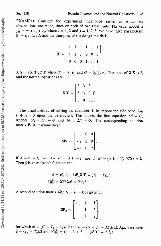
Sec. 2.8] Pseudo-Inverses and the Normal Equations 25
EXAMPLE. Consider the experiment mentioned earlier in which sixobservations are made, three on each of two treatments. The usual model isy;f = m + t, + eij where i = 1, 2 and j = 1, 2, 3. We have three parameters:(3' = (m, t l , t2), and the transpose of the design matrix is
1 1 1 1 1 1
X'= 1 1 1 0 0 0;
0 0 0 1 1 1
X'Y = (G, T1 , T2)' where Ti = y and G = I t Ij yij . The rank of X'X is 2,and the normai equations are
6 3 3
X'Y = 3 3 0 .
3 0 3
The usual method of solving the equations is to impose the side conditiont l + t2 = 0 upon the parameters. This makes the first equation 6m = G,whence 611 = 2T1 — G and 612 = 2T2 — G. The corresponding solutionmatrix P l is unsymmetrical.
1 0 0
6P1 = --1 2 0
— 1 0 2
If zG = tl — t, we have X' = (0, 1, —1) and, if 3r' = (0, 1, —1), X'Xr = a.Then 0 is an estimable function and
^ = (0, 1, — 1)P1X'Y = (T1 — T2)/3 ,
V(^) = a'P1a72 = 2a2 /3.
A second solution matrix with t l + t2 = 0 is given by
1 1 1
12P2 = 1 1 —3
1 —3 1
for which m = (G + Tl + T2)/12 and 11 = (G + Tl — 3T2)/12. Again we have+^ = (Ti — T2)/3 and V(^) = (1 + 3 + 3 + 1)02/12 = 2a2/3.
Dow
nloa
ded
12/1
1/12
to 1
29.1
28.2
07.2
42. R
edis
trib
utio
n su
bjec
t to
SIA
M li
cens
e or
cop
yrig
ht; s
ee h
ttp://
ww
w.s
iam
.org
/jour
nals
/ojs
a.ph
p

26 Linear Models and Quadratic Forms [Ch. 2
Two other solution matrices having t 2 = 0 and t l = (T1 — T2)/3 are given by
00 1 0 0 1
3P3 = 0 1 —1 , 3P4 = 0 1 —1
0 0 0 1 —1 —1
These give the same results as before for and V(^).In this example the estimable functions are 0 1 = m + t 1 , 1s = m + t 2 , and
any linear combination of them, including in particular 0 3 = tl — t2 .
2.9 Solving the Normal Equations
In the example given in the previous section, we solved the normal equationsby imposing a side condition upon the parameters. The side condition t l + t2 = 0,or Zl + t2 = 0, added an extra equation to the normal equations, which thengave us a set of p + 1 equations of which p were linearly independent. Anynonestimable linear function of the parameters can be used as a side conditlon.For example, m = 0 or t l = 0 or t2 = 0 would each sufface. So, for that matter,would a bizarre linear combination such as 72m + 13t 1 + 97t2 = 0; theequations would not be convenient to solve and the estimates of m, t 1 , and t2
would look a little peculiar, but it should be emphasized that the estimates ^of the estimable functions 0 would be the same no matter which of the sideconditions was imposed. The usual procedure. is to choose a side conditionwhich enables us to obtain a solution matrix P and a solution vector (3 asconveniently as possible.
We present now two standard methods of obtaining solution matrices in thecase where r(X) = k = p — m and m > 0, with a set of m side conditions. Forthose experiments in which the normal equations have a simple form, the solu-tion matrix is easily obtained directly; the reader may, therefore, wish topostpone this section until he reaches Chapter 11.
Let D be a matrix ofp rows and m columns such that r(D) = m and XD = 0.Suppose allo that we add m further rows to X in the form of a matrix H of mrows and p columns, such that the rank of (X', H') is p. Then HD is nonsingular.If the normal equations are solved, subject to the side conditions H13 = 0, thesolutions ft are unique numerically. However, since D'X'Y = 0, the solutionsmay differ in form by some linear combination of the rows of D'X'Y.
In the previous example, D' = (1, —1, —1) and D'X'Y = G — Tl — T2 - 0.The solutions are obtained with H = (0, 1, 1). The solution matrix P l givesµ = G/6; P2 gives µ = (G + Tl + T2)/12 = (G/6) — (D'X'Y/12).
Let P and P* be two solution matrices under the side conditions Hp = 0.Then PX'Y = P*X'Y. This is an identity in Y, and so (P — P*)X' = 0. Butr(X) = (p — m), and r(D) = m. Thus, if W is a matrix such that XW = 0,there exists a matrix E such that W = DE', and so P — P* = ED'. If P and P*
Dow
nloa
ded
12/1
1/12
to 1
29.1
28.2
07.2
42. R
edis
trib
utio
n su
bjec
t to
SIA
M li
cens
e or
cop
yrig
ht; s
ee h
ttp://
ww
w.s
iam
.org
/jour
nals
/ojs
a.ph
p
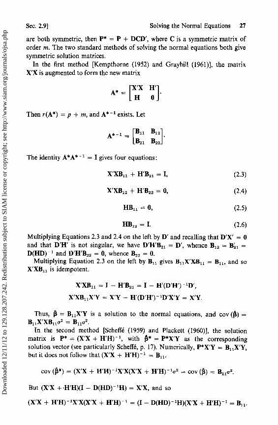
Sec. 2.9] Solving the Normal Equations 27
are both symmetric, then P* = P + DCD', where C is a symmetric matrix oforder m. The two standard methods of solving the normal equations both givesymmetric solution matrices.
In the first method [Kempthorne (1952) and Graybill (1961)], the matrixX'X is augmented to form the new matrix
A* = [XIX H'1H 0
Then r(A*) = p + m, and A* -1 exists. Let
A* _1 = B11 B12
B21 B22] .
The identity A*A* -1 = I gives four equations:
X'XB11 + H'B21 = I, (2.3)
X'XB12 + H'B22 = 0, (2.4)
HB11 = 0, (2.5)
HB12 = I. (2.6)
Multiplying Equations 2.3 and 2.4 on the left by D' and recalling that D'X' = 0and that D'H' is not singular, we have D'H'B 21 = D', whence B12 = B'21 =D(HD) -1 and D'H'B22 = 0, whence B22 = 0.
Multiplying Equation 2.3 on the left by B 11 gives B 11X'XB11 = B, and soX'XB11 is idempotent.
X'XB11 = I — H'B21 = I — H'(D'H') -1D',
X'XB11X'Y = X'Y — H'(D'H') -1D'X'Y = X'Y.
Thus, (3 = B 11X'Y is a solution to the normal equations, and cov () _B11X'XB11a2 = B1la2 .
In the second method [Scheffé (1959) and Plackett (1960)], the solutionmatrix is P* = (X'X + H'H) -1 , with 0* = P*X'Y as the correspondingsolution vector (see particularly Scheffé, p. 17). Numerically, P*X'Y = B 11X'Y,but it does not follow that (X'X + H'H) -1 = Bl1.
cov (*) = (X'X + H'H) -1X'X(X'X + H'H) - lo2 = cov (^) = Bllv2 .
But (X'X + •H'H)(I — D(HD) -1H) = X'X, and so
(X'X + H'H) -1X'X(X'X + H'H) -1 = (I — D(HD) -1H)(X'X + H'H) -1 = B11.
Dow
nloa
ded
12/1
1/12
to 1
29.1
28.2
07.2
42. R
edis
trib
utio
n su
bjec
t to
SIA
M li
cens
e or
cop
yrig
ht; s
ee h
ttp://
ww
w.s
iam
.org
/jour
nals
/ojs
a.ph
p

28 Linear Models and Quadratic Forms [Ch. 2
This gives us a method of obtaining B 11 from (X'X + H'H) -1 . We cannot,however, obtain (X'X + H'H) -1 from B11 with this result because
(1— D(HD) -1H)
is idempotent, and thus is not of full rank.We now obtain a different relationship between the two solution matrices.
We write (X'X + H'H) -1 = B11 + DCD'. Then
I = (X'X + H'H)(B ll + DCD') = X'XB ll + H'HDCD'
= I — H'(D'H') - 'D' + H'HDCD',
and so H'(D'H') -1D' = H'HDCD'. Multiplying both lides on the left by(D'H') - 'D' and on the right by H'(D'H') -1 reduces this equation [John (1964)a]to
(D'H')-1 = HDC,
whence
C = (HD) - '(D'H') - ' = (D'H'HD) -1 ,
so that
(X'X + H'H) -' = B11 + D(D'H'HD) - 'D'.
2.10 A Theorem in Linear Algebra
The following theorem will be used later in proving Cochran's theorem.Alternative proofs of the theorem and other relevant results are given by James(1952), Lancaster (1954), Graybill and Marsaglia (1957), and Banerjee (1964).
Theorem 1. Let Al„, Ak be symmetrie matrices of order n such thatI = ^i= 1 Â. Each of the following conditions is necessary and sufficient for theother two:
(i) All the Ai are idempotent;(ii) A,A; = Ofor all pairs i, j, i s4 j;(iii) Ii n, = n where n i = r(Ai).
PROOF . There is an orthogonal matrix P such that
k
P'IP = I = P'A 1P + P'AJP,t=z
where
P'A'P = (0 0)and P'A,P = (B; Cl)
i r
Dow
nloa
ded
12/1
1/12
to 1
29.1
28.2
07.2
42. R
edis
trib
utio
n su
bjec
t to
SIA
M li
cens
e or
cop
yrig
ht; s
ee h
ttp://
ww
w.s
iam
.org
/jour
nals
/ojs
a.ph
p

Sec. 2.111 The Distribution of Quadratic Forms 29
where A is the diagonal matrix whose diagonal elements are the nl nonzerolatent roots of A l , and B; is a square matrix of order n l . Throughout this proof,j takes the values 2 <— j 5 k.
Suppose all the A. are idempotent. To establish condition (ii), it is enough toshow that A,A; = 0 for all j. We have A = I and 1, tr (Bi) = 0; but P'AfPis idempotent, and so the diagonal elements of B ; cannot be negative. HenceB1 = 0 and C, = 0 for each j. It follows that A 1A, = PP'A1 PP'A1P = 0.
Since P'A;P is idempotent, E; is idempotent. Then n = tr (In) = nl +1 tr (E;) = n l + 1 nf, and condition (iii) is established.
We now show that conditions (ii) and (iii) each imply condition (i). SupposeA,A1 = 0 for all pairs i, j where i j. Then for each i,
A;= AtiI= A{(A1+ . ..+Ai+...+A,j=A,.
If condition (iii) holds, we can show that A l is idempotent. We write B, C, E, Qfor 1 Bj, 1 Cj, E5, 1 A;. Then, since P'A 1P + P'QP = I, we have E = In_n1,C = 0. But r(P'QP) = r(Q) = n — n l = r(E), and so B = 0 and A = I, sothat A l is idempotent. u
2.11 The Distribution of Quadratic Forms
If Y is a vector of N random variables, the quadratic form Y'AY is also arandom variable. Most of the results in this section about the distribution ofquadratic forms hold only when Y has the multivariate normal distribution.The following lemma is true even when the yl are not normally distributed.
Lemma. Let E(Y) = p and cov (Y) = Io2. Then E(Y'AY) = µ'Aµ + a2 tr (A).
PROOF.
Y'AY = a, t yi + 2 at,yty>>t i <1
E(y) = µi + a2 , E(ytyf) = µtlif•
Hence,
E(Y'AY) _ aµ41 + at1Q2 + 2 a115 = &'AN. + a2 tr (A). •t i t f
t<1
The next result concerns the normal distribution.
Theorem 1. Let Y — N(µ, I). The moment generating function of Y'AY isMy.Ay(t) = II — 2AtJ -1/2 exp{ — IIµ'µ — µ'(I — 2At) -1g)}.
Dow
nloa
ded
12/1
1/12
to 1
29.1
28.2
07.2
42. R
edis
trib
utio
n su
bjec
t to
SIA
M li
cens
e or
cop
yrig
ht; s
ee h
ttp://
ww
w.s
iam
.org
/jour
nals
/ojs
a.ph
p

30 Linear Models and Quadratic Forms [Ch. 2
PROOF . Suppose X — N(U, V). The probability density function of X is
.1x (X) = (21r)N12 [V 1 112 exp{ — 1(X — U)' V - 1(X — U)},
and the corresponding multiple integral over the range —00 <X < +00 isunity. The moment-generating function of Y'AY is
E[e<Y"AY] = (2^.) - Nj2 J - exp{— [(Y — µ)'(Y — µ) — 2tY'AY]/2} dY.m
Writing the exponent as — Q/2, we have
Q=Y'(I-2tA)Y—Y'µ— .'Y+µ'...
Completing the square and writing U for (I — 2At)- 'g,
Q=(Y—U)'(I-2At)(Y—U)+µ'(I—(I-2At) -1)µ,
so that
M(t) = (21T) - N 12 f 00 exp{—I(Y — U)'(I — 2At)(Y — U)}
dY exp[—µ'(I — (1 — 2At) - ')K/2]
= ^I — 2At^ - 112 exp(—+[i'p. — (I — 2At) - fit]}• E
If A = I, we have for the moment-generating function of Y'Y
My ,y(t) = (1 — 2t) - N 12 exp[—,1 + a(1 — 2t) -1 ].
This is the moment-generating function of the noncentral X2 distribution withN d.f. and noncentrality parameter A = µ'µ/2. If A = I and µ = 0, M(t) =(1 — 2t) - N 12, which is the moment-generating function of the centra! X2distribution with N d.f.
If cov (Y) = V, we may prove in similar fashion that
M(t) = II — 2tAVI -1 /2 exp{—I[µ'V - lµ — µ'V -1(I — 21VA) - lµ]}.
The next theorem points out the importante of idempotent matrices in thetheory of the distribution of quadratic forms.
Theorem 2. Let Y — N(µ, I). A necessary and sufficient condition that Y'AY havea X2 distribution with m < N d.f. is that A be an idempotent matrix of rank m.
Dow
nloa
ded
12/1
1/12
to 1
29.1
28.2
07.2
42. R
edis
trib
utio
n su
bjec
t to
SIA
M li
cens
e or
cop
yrig
ht; s
ee h
ttp://
ww
w.s
iam
.org
/jour
nals
/ojs
a.ph
p
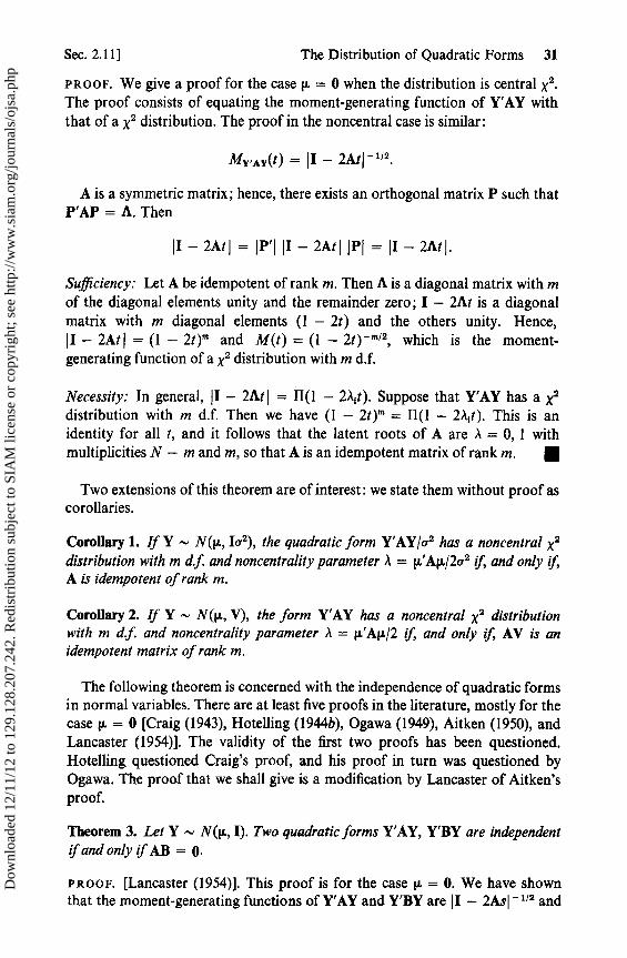
Sec. 2.11] The Distribution of Quadratic Forms 31
PxooF. We give a proof for the case µ = 0 when the distribution is central X2.
The proof consists of equating the moment-generating function of Y'AY withthat of a X 2 distribution. The proof in the noncentral case is similar:
MY.nx(t) = ]I — 2Atj -112.
A is a symmetrie matrix; hence, there exists an orthogonal matrix P such thatP'AP = A. Then
I — 2At I = IP'I II — 2At HPI = II — 2At I.
Sufficiency: Let A be idempotent of rank m. Then A is a diagonal matrix with mof the diagonal elements unity and the remainder zero; I — 2At is a diagonalmatrix with m diagonal elements (1 — 2t) and the others unity. Hence,]I — 2At = (1 — 2t)m and M(t) = (1 — 2t) - m/2, which is the moment-generating function of a x2 distribution with m d.f.
Necessity: In general, I — 2At = 1I(1 — 21,t). Suppose that Y'AY has a Xadistribution with m d.f. Then we have (1 — 2t)m = 1I(1 — 2),t). This is anidentity for all t, and it follows that the latent roots of A are A = 0, 1 withmultiplicities N — m and m, so that A is an idempotent matrix of rank m. u
Two extensions of this theorem are of interest: we state them without proof ascorollaries.
Corollary 1. 1f Y — N(µ, Ia2), the quadratic form Y'AY/a2 has a noncentral X2
distribution with m d.f. and noncentrality parameter A = µ'Aµ/2a 2 if, and only if,A is idempotent of rank m.
Corollary 2. 1f Y — N(µ, V), the form Y'AY has a noncentral x2 distributionwith m d.f. and noncentrality parameter A = µ'Aµ/2 if, and only if, AV is anidempotent matrix of rank m.
The following theorem is concerned with the independence of quadratic formsin normal variables. There are at least five proofs in the literature, mostly for thecase µ = 0 [Craig (1943), Hotelling (1944b), Ogawa (1949), Aitken (1950), andLancaster (1954)]. The validity of the first two proofs has been questioned.Hotelling questioned Craig's proof, and his proof in turn was questioned byOgawa. The proof that we shall give is a modification by Lancaster of Aitken'sproof.
Theorem 3. Let Y — N(1r., I). Two quadratic forms Y'AY, Y'BY are independentifandonlyifAB = 0.
PROOF. [Lancaster (1954)]. This proof is for the case µ = 0. We have shownthat the moment-generating functions of Y'AY and Y'BY are 11 — 2AsI -112 and
Dow
nloa
ded
12/1
1/12
to 1
29.1
28.2
07.2
42. R
edis
trib
utio
n su
bjec
t to
SIA
M li
cens
e or
cop
yrig
ht; s
ee h
ttp://
ww
w.s
iam
.org
/jour
nals
/ojs
a.ph
p

32 Linear Models and Quadratic Forms [Ch. 2
11 — 2Bt1 -112 . By a similar argument, the joint moment-generating function ofthe two forms is seen to be 1I — 2As — 2Bt 1 -1 "2 . We have to show that thejoint function is the product of the two individual functions, i.e.,
^I— 2Asj]I-2BtI=^I— 2As —2BtI, (2.3)
for all values of s and t in an interval around the origin if, and only if, AB = 0.The sufficiency part is trivial since, if AB = 0, we have
^I-2AsJ I-2BtI = ^I— 2As —2Bt+4ABst = ^I-2As-2BtI.
Conversely, suppose Equation 2.3 is true. Let P be an orthogonal matrix suchthat
P'AP = (A 0
P'BP = (C21
C^^ C^2l`0 0) — C22
where A is diagonal and A and C11 are square matrices of order r(A). It followsfrom Equation 2.3 that for any ,1 0 we may replace s by s/A and t by t/)) toobtain
IJ-2AsH Ju-2BtI = a"IM-2As-2BtI
or
^1I — 2P'APs — 2P'BPtI — 2P'APs — 2P'BPtI.
Equating coefficients of st( ) on each side of the equation gives
Al — 2 P'BPt 1= PA) 1 M- 2 C22 t 1.
Thus P'BP and C22 have the same nonzero latent roots. This implies that thesum of the squares of elements of P'BP is equal to the sum of the squares of theelements of C22 , each being the sum of the squares of the latent roots. Since allthe elements of B are real, this implies that C l„ Cr2, and C21 are all zero matricesso that P'APP'BP = 0 and AB = 0.
In the case g 0, we must, in addition, take into account the exponents in themoment-generating functions. Thus we must show that
..'{I — (I — 2As) -1}µ + N.'{I — (I — 2Bt) - '}p. = 1.'{I — (I — 2As — 2Bt) -1}g
for all s and t in some interval containing s = t = 0, i.e.,
I—(I-2As) -1 +I—(I-2Bt) -1 =I—(I-2As-2Bt) -1 ,
if, and only if, AB = 0.
Dow
nloa
ded
12/1
1/12
to 1
29.1
28.2
07.2
42. R
edis
trib
utio
n su
bjec
t to
SIA
M li
cens
e or
cop
yrig
ht; s
ee h
ttp://
ww
w.s
iam
.org
/jour
nals
/ojs
a.ph
p

Sec. 2.11 ] The Distribution of Quadratic Forms 33
For sufficiently small s we have
I — (I — 2As) - = I — (I + 2As + (2 As) 2 + ... + (2As)" + ... ),
and the required condition becomes
2As +(2As) 2 +••• + 2Bt +(2Bt)2 +•••
= (2As + 2Bt) + (2As + 2Bt)2 +...
Equating coefficients, this is true if, and only if, AmBnsmtn = 0 for all m, n, andfor all s, t, which in turn is true if, and only if, AB = 0. 3
In the analysis of variance, Y'Y is subdivided into several quadratic forms(sums of squares). The next theorem is concerned with the joint distribution ofthese sums of squares. It is due to Cochran (1934) and is essentially an algebraicresult expressed in a statistical context. He originally proved it in the centra!case. The noncentral case is due to Madow (1940).
Theorem 4. Let Y — N(p., 1) and let Y'Y = Y'A 1Y + • • • + Y'A,,Y where Yhas n observations and r(A 1) = n i . A necessary and sufficient condition for theforms Y'A,Y to be distributed independently with Y'A,Y— X2(ni) is that 1 n, = n.
PROOF. We have already shown that n { = n if, and only if, each A, is idem-potent and if, and only if, AAf = 0 where i s4 j. But A i idempotent is equivalent toY'A,Y _ X2(ni), and AA, = 0 is equivalent to Y'A,Y and Y'A 1Y independent. •
We may rephrase the statement of the theorem in the following way. LetY — N(p., I), and let Y'Y = 1 Y'A,Y where r(Ai) = n i. Then any one of thefollowing five conditions implies the other four:
(i) ni = n;(ii) Each At is idempotent;
(iii) A,A1 = 0 for all pairs i, j, where i 0 j;(iv) Y'A1Y — x2(ni) for each i;(v) Y'A{Y, Y'A5Y are independent for all i, j where i # j.
Each of the forms Y'A,Y may be written as Y'Bi'B1Y where Bt is a matrix of n,rows and n columns such that B,B! = I74 i.e., such that the columns of Bi forman orthonormal set of ni vectors, It follows from the fact that A tA; = 0 thatBBI' = 0 also, for we have
A1A5 = BiB,BJBJ = 0,
and, multiplying on the left by B i and on the right by Bi,
IB,B f'I = B{B! = 0.
Let B be the matrix defined by B' = (B'1 , Bi,. . . ). Then B is an orthogonalmatrix, and the transformation Z = BY is an orthogonal transformation takingY'Y into Z'Z.
Dow
nloa
ded
12/1
1/12
to 1
29.1
28.2
07.2
42. R
edis
trib
utio
n su
bjec
t to
SIA
M li
cens
e or
cop
yrig
ht; s
ee h
ttp://
ww
w.s
iam
.org
/jour
nals
/ojs
a.ph
p
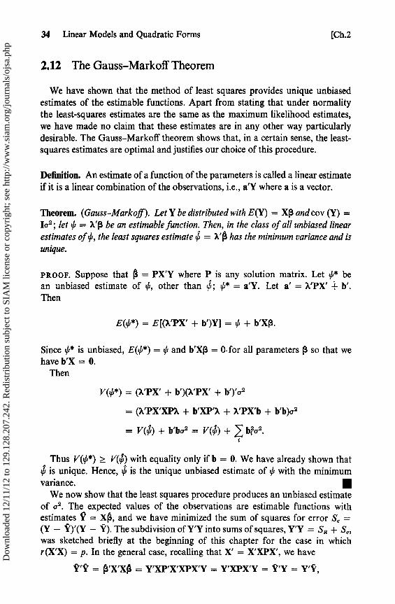
34 Linear Models and Quadratic Forms [Ch.2
2.12 The Gauss—Markoff Theorem
We have shown that the method of least squares provides unique unbiasedestimates of the estimable functions. Apart from stating that under normalitythe least-squares estimates are the same as the maximum likelihood estimates,we have made no claim that these estimates are in any other way particularlydesirable. The Gauss—Markoff theorem shows that, in a certain sense, the least-squares estimates are optimal and justifies our choice of this procedure.
Definition. An estimate of a function of the parameters is called a linear estimateif it is a linear combination of the observations, i.e., a'Y where a is a vector.
Theorem. (Gauss—Markoff). Let Y be distributed with E(Y) = X(3 and cov (Y) _Ia2 ; let 0 = a'(3 be an estimable function. Then, in the class of all unbiased linearestimates of b, the least squares estimate = ai has the minimum variance and isunique.
PROOF. Suppose that 0 = PX'Y where P is any solution matrix. Let 0* bean unbiased estimate of 0, other than ; * = a'Y. Let a' = )'PX' 4- b'.Then
E(O*) = E[(a'PX' + b')Y] = :G + b'Xp.
Since :G* is unbiased, E(*) = 0 and b'Xp = 0. for all parameters [i so that wehave b'X = 0.
Then
V(O*) = (a'PX' + b')(a'PX' + b')'a 2
= (a'PX'XPa + b'XP'a + )^'PX'b + b'b)a 2
= V(^) + b'bo2 = V(^) + bi a2 .
Thus V(/*) >_ V(+) with equality only if b = 0. We have already shown thatis unique. Hence, is the unique unbiased estimate of 0 with the minimum
variance. uWe now show that the least squares procedure produces an unbiased estimate
of a2. The expected values of the observations are estimable functions withestimates Y = X^i, and we have minimized the sum of squares for error Se =(Y — — Y). The subdivision of Y'Y into rums of squares, Y'Y = SR + Se ,was sketched briefly at the beginring of this chapter for the case in whichr(X'X) = p. In the general case, recalling that X' = X'XPX', we have
yl' = ^i'X'XO = Y'XP'X'XPX'Y = Y'XPX'Y = Y'Y = Y'Y,
Dow
nloa
ded
12/1
1/12
to 1
29.1
28.2
07.2
42. R
edis
trib
utio
n su
bjec
t to
SIA
M li
cens
e or
cop
yrig
ht; s
ee h
ttp://
ww
w.s
iam
.org
/jour
nals
/ojs
a.ph
p

Sec. 2.12] The Gauss—Markoff Theorem 35
and
Se =Y'Y—Y"'—i'Y+' 't = Y'(I — XPX')Y,
SR = Y'XPX'Y = ^3'X'Y.
Since E(Y) = X(d and cov (Y) = Ia',
E(Y'Y) = (3'X'1X13 + a 2 tr (I) = f3'X'X(3 + Na2 ,
and
E(SR) = E(Y'XPX'Y) = E3'X'XPX'XR + a 2 tr (XPX').
XPX' is idempotent, and so tr (XPX') = r (XPX'). Now r (XPX') < r (X) = k;but X' = X'XPX', and so r(X) = r(X') < r(XPX'). Hence, r(XPX') _r(X) = k, and we have
E(SR) = f'X'X13 + ka2 ,
and, by subtraction,
E(Se) = (N — k)a2 .
Thus, we see that the sum of squares for error provides an unbiased estimateS2 = Se/(N — k) of the error variance a2 .
The matrices XPX' and (I — XPX') of the quadratic forms SR, SQ are bothidempotent. Under normality, the conditions of Cochran's theorem are satisfiedif we replace Y by o - 1Y, and so SR/a2 and Se/o2 have independent X 2 distribu-tions with k and (N — k) d.f. respectively.
2.13 Testing Hypotheses
Throughout this section we shall assume that Y has a multivariate normaldistribution. The distribution of SR/aa is noncentral x2 with noncentralityparameter f'X'X f /(2o 2). Thus, as we have already mentioned, an appropriatetest statietic for the nul! hypothesis H o : (i = 0 against the general alternative
p # 0 (i.e., at least one of the elements of p is not zero) is = k - 'SR/(N — k) - 'Se , where k = r(X). Under the nuli hypothesis, . has Snedecor's Fdistribution with k and (N — k) d.f. The critical region is the upper tail ofF(k, N — k). We shall not discuss here the optimum properties of the F testin this situation. The reader who wishes to pursue the matter further is referred toScheffé (1959), especially Chapter 2.
When a sum of squares is divided by the number of degrees of freedom in thecorresponding x2 distribution, the quotient is called a mean square. Thus, S 2 is themean square for error, and SR/k is the mean square for regression.
Dow
nloa
ded
12/1
1/12
to 1
29.1
28.2
07.2
42. R
edis
trib
utio
n su
bjec
t to
SIA
M li
cens
e or
cop
yrig
ht; s
ee h
ttp://
ww
w.s
iam
.org
/jour
nals
/ojs
a.ph
p

36 Linear Models and Quadratic Forms [Ch. 2
It may be argued that in some practical situations the hypothesis t = 0 is notespecially interesting, and the experimenter might be more interested in testingeither the hypothesis that some particular estimable function is zero or thehypothesis that all the parameters in some subset of P are zero.
Consider first a particular estimable function 0 = ?'[3, which is estimated by= a = >.'PX'Y. Then 2 = Y'XP'XX'PX'Y, and 2/(a'Pao2) has a X2
distribution with one d.f. Furthermore, X'(I — XPX') = 0, and so 2/(a'Paa2)and Se /a2 have independent X2 distributions. Thus, the hypothesis H 0 : 0 = 0may be tested by the F test using the test statistic F = 2/(X'PXs2), or, equiva-lently, by the t test with t 2 = F. Confidence intervals for 0 can be constructedusing Student's t in the usual way. For example, a two-sided interval could beobtained as
tÍi — t*()'Ps2)-1I2 ^ ,/, + t*(Á'P%ls2)-1I2
More will be said on this topic later.We next consider testing hypotheses of the type Ho : P l = 0 where p 1 is a
subvector of P. Suppose that (3 is divided into two subvectors, P = «1, 02), andthat X is similarly partitioned into (X 1 , X2). Let r(X i) = kl , r(X2) = k2. Thecomplete model for which we have just estimated the parameters is
Y = (X1, X2)(P1, f32) + e.
Under the hypothesis Ho : (3 1 = 0, we have the reduced model
Y=X202+e.
We write SR(P2), SR(P) for the sums of squares for regression under thereduced and complete models, respectively, and SR(P1IP2) for the differenceSR(P) — SR(P2). Let M be a solution matrix for the reduced normal equationsX2Y = X' X2 (32 i X2MX2 is idempotent and SR(P2) = Y'X2MX2Y.
We now have a subdivision of Y'Y into three quadratic forms:
Y ' Y = SR\N2) + SR(P1I P2) + Se,
where SR(P11 r2) = Y'(XPX' — X2MX2)Y.Now X' = X'XPX', and so X2 = X' XPX', and (XPX' — X 2MX2) is idem-
potent. Thus, SR(P2)/a 2, SR(P1 1 f32)/a2, Se /a2 have independent x 2 distributionswith k2 , k — k2 and N — k d.f. The hypothesis H0 : [i l = 0 is tested by com-paring the sum of squares for error under the reduced model, S e + SR(al Ito the sum of squares for error, Se , under the complete model, ad asking our-selves whether the reduction in error, SR([3 1 1(3 2), made by including P l in themodel is large enough to be regarded as significant. The test statistic F =(k — k2) -1SR(P11P2)/s2 has the F[k — k2, N — k] distribution under the nullhypothesis.
Dow
nloa
ded
12/1
1/12
to 1
29.1
28.2
07.2
42. R
edis
trib
utio
n su
bjec
t to
SIA
M li
cens
e or
cop
yrig
ht; s
ee h
ttp://
ww
w.s
iam
.org
/jour
nals
/ojs
a.ph
p

Sec. 2.14] Missing Observations 37
2.14 Missing Observations
It occasionally happens that in an experiment one or more of the observationsis spoiled or omitted. One might have planned a setup in which there wereseveral cars and several gasolines, each gasoline to be used in each car (a nicelybalanced experiment) only to find that something went wrong. Perhaps one ofthe cars broke down before being used to test all the gasolines and could not berepaired in time; perhaps, because of a failure in communications, not enoughof one of the fuels was prepared and the supply ran out before it could be testedin every car; perhaps one of the observations is so clearly incompatible with theothers that it should be rejected as containing gross error. What can be done?If possible, the experimenter should try to take another observation duplicatingthe experimental conditions prescribed for the missing observation. If thiscannot be done, we ask the following question: can we obtain a convenientformula or recipe for generating from the actual data an estimate for what themissing value should have been? Because this question first arose in agriculturalexperimentation [Yates (1933)] where the experimental units are called plots,these formulae are called missing plot formulae in the literature. We shall discussthe general case in this section. Specific formulae for lome of the standarddesigns will be given in later chapters, either in the text or as exercises.
Suppose that the experimental plan called for N + 1 observations or plots.We have N observations, Y, for which the design matrix is X (N x p). The(N + l)th observation is missing; its design matrix is a single row x. We shallchoose for our estimate of the missing observation the value y that minimizes thesum of squares for error when we carry out the least squares procedure for all(N + 1) points (the N actual data and y).
Writing 0 for the vector of estimates obtained in this way, we minimize
Se =(Y—XO)'(Y—XÇ3)+(y—x0) 2 .
The first term is minimized if we take 0 to be any solution vector to the normalequations for the N actual data points, and the second term is zero if we takey=x0.
From an abstract point of view we appear to have gained nothing except tosay that the best estimate y is obtained by solving the normal equations for theactual data and substituting 0 for (3 to obtain y = x^i. In practice, however, thedesign matrix (X', x')' is usually chosen in such a way that the augmentednormal equations can be solved very easily, whereas the equations X'X[3 = X'Ymay be more awkward to handle computationally. Since y — x^3 = 0, anequivalent procedure, which we shall use later, is to choose for y the value thatwill fit the model with zero residual when the least squares procedure is carriedout on the set of (N + 1) points consisting of the N data points and the missingplot (x, y).
Dow
nloa
ded
12/1
1/12
to 1
29.1
28.2
07.2
42. R
edis
trib
utio
n su
bjec
t to
SIA
M li
cens
e or
cop
yrig
ht; s
ee h
ttp://
ww
w.s
iam
.org
/jour
nals
/ojs
a.ph
p
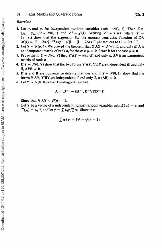
38 Linear Models and Quadratic Forms [Ch. 2
Exercises
1. Let y l and ya be independent random variables each N(µ, 1). Then Z =(Y — Y2)/V2 — N(0, 1) and Z 2 _ X2(1). Writing Z 2 = Y'AY where Y' =(Yi, Ya) show that the expression for the moment-generating function of Z 2 :M(t) = II — 2Atj -1 j2 exp —µ'{I — (I — 2At) -1}µ/2 reduces to (1 — 2t) -112 .
2. Let Y — N(µ, I). We proved the theorem that Y'AY — X 2(n,), if, and only if, A isan idempotent matrix of rank n, for the case µ = 0. Prove it for the case ^ 0.
3. Prove that if Y — N(0, V) then Y'AY — X 2(n) if, and only if, AV is an idempotentmatrix of rank n.
4. If Y — N(0, V) show that the two forms Y'AY, Y'BY are independent if, and onlyif, AVB = 0.
5. If A and B are nonnegative definite matrices and if Y — N(0, I), show that theforms Y'AY, Y'BY are independent, if and only if, tr (AB) = 0.
6. Let Y — N(0, D) where Dis diagonal, and let
A = D - ' — (D - 'JD -1/1'D -11).
Show that Y'AY — X2(n — 1).7. Let Y be a vector of n independent normal random variables with E(y) = µ, and
V(y ) = wr 1, and let y = 1 w,y,/> w,. Show that
1 ws(Y1 — 9)2 X2(n — 1).
Dow
nloa
ded
12/1
1/12
to 1
29.1
28.2
07.2
42. R
edis
trib
utio
n su
bjec
t to
SIA
M li
cens
e or
cop
yrig
ht; s
ee h
ttp://
ww
w.s
iam
.org
/jour
nals
/ojs
a.ph
p
CHAPTER 3
Experimentswith a
Single Factor
If an agronomist wishes to compare the yields of five varieties of wheat, anobvious procedure would be to mark off twenty plots of land and to sow varietyA on four of them, variety B on four more of them, and so on. The varieties areassigned to the plots by some random procedure, and from each plot comes asingle observation, the yield on that plot. This simple experiment is called acompletely randomized experiment because of the method of assigning thevarieties. We shall begin our discussion of experimental designs by consideringthis kind of experiment.
An industrial example would be the comparison of four different operatingtemperatures on the yield of a product from a chemical reactor. Twenty runscould be made, five at each temperature, and the yield of product at each runrecorded. Again, the temperatures should be assigned to the runs at random.Suppose that the process involves the use of an acid catalyst which deteriorateswith time. If the experimenter were to make the runs at the highest temperaturefirst, then the runs at the next highest temperature, and finally the runs at thelowest temperature, he would have difficulty interpreting his results. If the yieldsat the high temperatures were greater than the yields at low temperatures, couldhe be sure whether the apparent drop in yield resulted from the reduction in theoperating temperature or from the deterioration of the acid? The random assign-ment of the temperatures to the runs, or of the varieties to the plots, is essential toour analysis of the experiment. The models for the experiments will be linearmodels like those of the last chapter. In the model for each observation therewill be an error term, e; these errors are assumed to be uncorrelated.
In general, a set of different treatments are applied to N experimental units,one treatment to each unit, and an observation is made on each unit. The
39
Dow
nloa
ded
12/1
1/12
to 1
29.1
28.2
07.2
42. R
edis
trib
utio
n su
bjec
t to
SIA
M li
cens
e or
cop
yrig
ht; s
ee h
ttp://
ww
w.s
iam
.org
/jour
nals
/ojs
a.ph
p

40 Experiments with a Single Factor [Ch. 3
theory of experimental design was first developed in agriculture and muchof the jargon is taken from that field. We shall refrain from using the expressionexperimental unit. Instead we shall most often use the agricultural term plot,or, when talking of industrial experiments, the terms run or point. An observationwill commonly be referred to as a yield or a response.
Some of our examples will be concerned with octane numbers. Producers ofgasoline are interested in the octane number of their product. If a driver uses agasoline with too low an octane number, the engine of his car will knock. Largercars with engines that have higher compression ratios need higher octane than docompact cars to prevent knocking. Thus, high octane number is a desirable charac-teristic of a gasoline. The octane number may be determined in the laboratory oron the road by a procedure that may be described in a simplified fashion as follows.
There is a standard engine on which the compression ratio may be varied.The engine is run with the gasoline to be tested. The compression ratio is in-creased until knocking occurs, and the reading on the meter is noted. Then theprocedure is repeated using reference fuels. These are mixtures of normalheptane and iso-octane. A reference fuel composed of X per cent iso-octane and(100 — X) per cent normal heptane is defined as having octane number X. Tworeference fuels are used, one with a slightly higher octane number than the un-known gasoline and one with a slightly lower octane number. The readings onthe compression ratio meter at which the engine knocks using each of thereference fuels are noted, and the octane number of the gasoline being tested isobtained by interpolation. An observed octane number is a random variable.A standard deviation of about 0.3 ON is not unusual.
A similar procedure can be followed using automobiles on the road to obtain"road-octane numbers." The manufacturers of both cars and gasolines conducttests under road conditions to find both the road-octane numbers of commercialgasolines and the octane requirements of commercial automobiles. Because themodern automobile engines differ somewhat from the standard engines, andfrom each other, and also because the components in commercial gasoline arenot iso-octane and normal heptane, it often happens that even apart fromrandom error a test fuel will have different octane ratings in different cars andthese ratings will differ from those obtained in the laboratory. The octane numberof a gasoline can be increased by the use of special additives such as tetra-ethyllead or tetra-methyl lead, or by adding some of the aromatic hydrocarbonsfound in crude oil. The latter, however, are also in demand for petrochemicals,and the managers of an oil company have to decide how much of their supplyshould be used for each purpose.
An engineer wishing to compare five gasolines might take twenty cars, assigneach gasoline to four cars, and observe the octane number for each car—gasolinecombination. The choice of cars is important to the analysis of the experimentand to the use of the results. One should not experiment solely on Volkswagensif the results are to be used to make decisions about Cadillacs, nor should oneexpect crops to yield the same amounts in the Central Valley of California asthey do in the coastal area.
Dow
nloa
ded
12/1
1/12
to 1
29.1
28.2
07.2
42. R
edis
trib
utio
n su
bjec
t to
SIA
M li
cens
e or
cop
yrig
ht; s
ee h
ttp://
ww
w.s
iam
.org
/jour
nals
/ojs
a.ph
p

Sec. 3.1 ] Analysis of the Completely Randomized Experiment 41
3.1 Analysis of the Completely Randomized Experiment
In either of the two experiments just mentioned we can take as a model
yij= µs +e15, i= 1, 2,...,t;j= 1,2,...,r,
where y{f denotes the jth observation on the ith gasoline, or the yield on the jthof the plots that were sown with the ith variety of wheat, µ, denotes the " true "value of the octane number or the yield of the ith gasoline or variety; i.e.,E(y15), and e15 is the random error of the (ij)th observation or plot. We assumethat the µ, are unknown constants, and that the e11 are uncorrelated randomvariables, each distributed with the same mean, zero, and the same variance Q2 .
We use the general term treatments for the gasolines or the varieties and speak ofan experiment with t treatments.
In addition we may make the normality assumption, namely that the elf arenormally distributed, i.e., the vector e of the e15 has a multivariate normaldistribution with mean vector 0 and covariance matrix Ia2 .
The least squares estimate of p-, which is the maximum likelihood estimateunder the normality assumption, is the average of the observations on the ithtreatment. Writing
G = y11, Ti = > y1j, y,. = Yt = Ti/r,{ r f
we have
11 = yt., (3.1)
Se = t(r — 1 )s2 = (Yti — y1.)2 = 2u — T2 /r. (3.2)s i s ! t
If the number of observations is not the same for each treatment, we denote thenumber of observations on the ith treatment by r, and let y,. = Tlr,. .ThenEquation 3.2 becomes Se = Ii Ii yi'i — l{ T,2/r1 .
We shall use N to denote the total number of observations, G for the grandtotal 1, Ii ytj of the observations, and y.. or y for the grand mean G/N. The casewhere ri = r for all i will be called the equireplicate case. (Some people like to saythat the ith treatment is replicated r, times; we shall do so when we considerincomplete block designs in a later chapter).
Under the normality assumption the hypothesis µ, = µ,. can be tested byStudent's t test. In the equireplicate case the test statistic
t = (yi — Y'i) (r/25 2 )
has, under the hypothesis, Student's t distribution with t(r — 1) d.f.
Dow
nloa
ded
12/1
1/12
to 1
29.1
28.2
07.2
42. R
edis
trib
utio
n su
bjec
t to
SIA
M li
cens
e or
cop
yrig
ht; s
ee h
ttp://
ww
w.s
iam
.org
/jour
nals
/ojs
a.ph
p
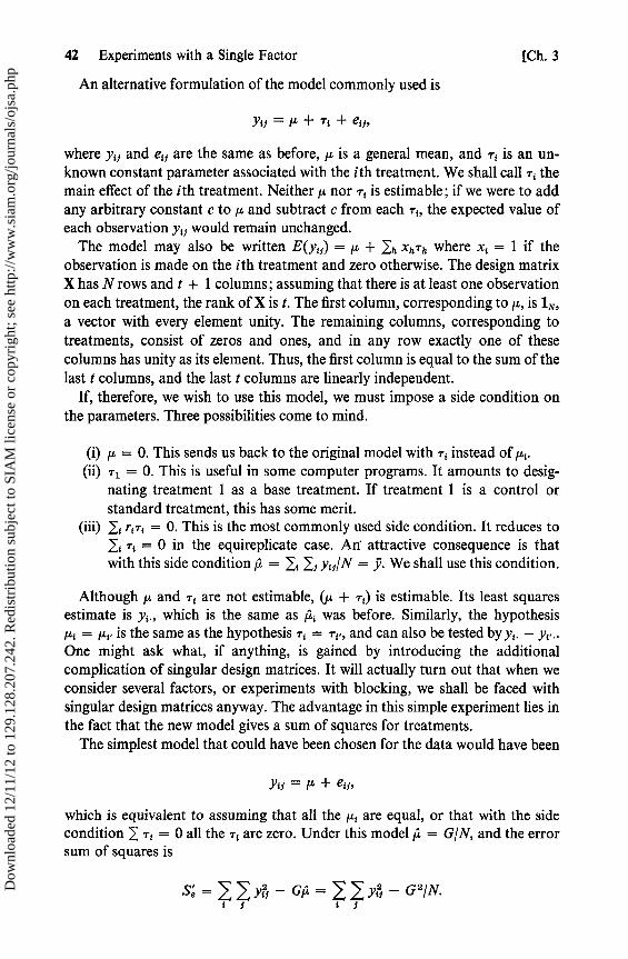
42 Experiments with a Single Factor [Ch. 3
An alternative formulation of the model commonly used is
yi=µ + ri + eu,
where yi and e15 are the same as before, µ is a general mean, and T{ is an un-known constant parameter associated with the ith treatment. We shall call -Ti themain effect of the ith treatment. Neither µ nor T{ is estimable; if we were to addany arbitrary constant c to and subtract c from each T,, the expected value ofeach observation yij would remain unchanged.
The model may also be written E(y 5) = µ + lh XhTh where x, = 1 if theobservation is made on the ith treatment and zero otherwise. The design matrixX has N rows and t + 1 columns; assuming that there is at least one observationon each treatment, the rank of X is t. The first column, corresponding to µ, is 1 N ,
a vector with every element unity. The remaining columns, corresponding totreatments, consist of zeros and ones, and in any row exactly one of thesecolumns has unity as its element. Thus, the first column is equal to the sum of thelast t columns, and the last t columns are linearly independent.
If, therefore, we wish to use this model, we must impose a side condition onthe parameters. Three possibilities come to mind.
(i) µ = 0. This sends us back to the original model with Ti instead of µ,.(ii) Tl = 0. This is useful in some computer programs. It amounts to desig-
nating treatment 1 as a base treatment. If treatment 1 is a control orstandard treatment, this has some merit.
(iii) 1t riri = 0. This is the most commonly used side condition. It reduces to1, -r, = 0 in the equireplicate case. An attractive consequence is thatwith this side condition µ = 1, If yij/N = y. We shall use this condition.
Although µ and Tt are not estimable, (µ + Ti) is estimable. Its least squaresestimate is y i ., which is the same as µ i was before. Similarly, the hypothesis
= . is the same as the hypothesis T, = -r,., and can also be tested by y1 . — yi...
One might ask what, if anything, is gained by introducing the additionalcomplication of singular design matrices. It will actually turn out that when weconsider several factors, or experiments with blocking, we shall be faced withsingular design matrices anyway. The advantage in this simple experiment lies inthe fact that the new model gives a sum of squares for treatments.
The simplest model that could have been chosen for the data would have been
ysi=µ+eu,
which is equivalent to assuming that all the µ i are equal, or that with the sidecondition 1 Ti = 0 all the -r, are zero. Under this model µ = G/N, and the errorsum of squares is
Sé= 1 — Gµ=yii — G 2/N.1 t 1
Dow
nloa
ded
12/1
1/12
to 1
29.1
28.2
07.2
42. R
edis
trib
utio
n su
bjec
t to
SIA
M li
cens
e or
cop
yrig
ht; s
ee h
ttp://
ww
w.s
iam
.org
/jour
nals
/ojs
a.ph
p

Sec. 3.1] Analysis of the Completely Randomized Experiment 43
When the treatment parameters r, are added to the model the estimate of µ isstil! µ. = y; the estimate of Tt is Tt = y,. — y, and the new sum of squares forregression is
SR = Gµ + Tfzt = G 2/N + TT(yc. — 9) _ T2/rr .i 1 t
The reduction in the sum of squares for error or the increase in the sum ofsquares for regression because of the addition of the treatment parameters to themodel is thus 1 T,a/r{ — G 2IN. This is called the sum of squares for treatmentsand is denoted by S. The sum of squares for error, Se , is the same as it was withthe first model.
We now have the subdivision of the sum of the squares of the observations
Y'Y = G 2/N + [> T?/r — G 2/N] + (y{r — y,•)2
or
Y'Y =C+St + Se .
The term G 2/N is called the correction for the mean and is often written asC. Y'Y is called the raw sum of squares; the corrected sum Y'Y — C is calledthe total sum of squares, and we shall occasionally denote it by ST .
The quadratic forms C, St, and Se have ranks 1, t — 1 and N — t respectively.Under normality they have, upon division by a2, independent chi-squaredistributions. The expected value of C is a2 + N -1(Nµ + r,-r,)2. 1f we write
rrr1 = NT, this becomes a2 + N(µ + T)2, and if we take the side conditionr,-r, = 0, E(C) reduces to u2 + Nµ2 . To compute E(St) we note that
E(Ti2/r1) = rt 'E(> e,! + riu + riT,) 2 = a2 + rt(N, + Tt)2 .i
Then
E(S) = (tal + Ng2 + 2µ rtT, + rir2) — E(C)_ (t — 1)a2 + r,(_, — T)a .
This information is summarized in Table 3.1.
TABLE 3.1ANALYSIS OF VARIANCE
Source SS d.f. EMS
Total Y'Y — C N— 1Treatments 7 /r, — C t — 1 a2 + (t — 1)' r{(r, — T)zError Y'Y — 7/r, N — t aaD
ownl
oade
d 12
/11/
12 to
129
.128
.207
.242
. Red
istr
ibut
ion
subj
ect t
o SI
AM
lice
nse
or c
opyr
ight
; see
http
://w
ww
.sia
m.o
rg/jo
urna
ls/o
jsa.
php
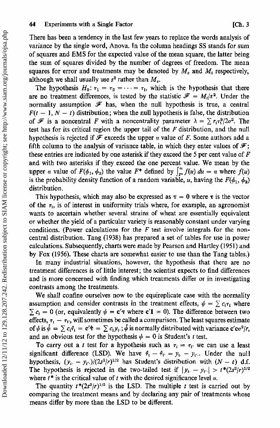
44 Experiments with a Single Factor [Ch. 3
There has been a tendency in the last few years to replace the words analysis ofvariance by the single word, Anova. In the column headings SS stands for sumof squares and EMS for the expected value of the mean square, the Jatter beingthe sum of squares divided by the number of degrees of freedom. The meansquares for error and treatments may be denoted by Me and Mt respectively,although we shall usually use s 2 rather than Me .
The hypothesis Ho : T l = T2 = • = Tt, which is the hypothesis that thereare no treatment differences, is tested by the statistic F = Mt/s 2. Under thenormality assumption F has, when the null hypothesis is truc, a centralF(t — 1, N — t) distribution; when the null hypothesis is false, the distributionof F is a noncentral F with a noncentrality parameter ,1 = r{ Ti /2a2. Thetest has for its critical region the upper tail of the F distribution, and the nullhypothesis is rejected if F exceeds the upper a value of F. Some authors add afifth column to the analysis of variance table, in which they enter values of F;these entries are indicated by one asterisk if they exceed the 5 per cent value of Fand with two asterisks if they exceed the one percent value. We mean by theupper a value of F(¢ l , ¢2) the value F* defined by fF f(u) du = a where f(u)is the probability density function of a random variable, u, having the F(¢ 1 , 02)distribution.
This hypothesis, which may also be expressed as r = 0 where T is the vectorof the i, is of interest in uniformity trials where, for example, an agronomistwants to ascertain whether several strains of wheat are essentially equivalentor whether the yield of a particular variety is reasonably constant under varyingconditions. (Power calculations for the F test involve integrals for the non-central distribution. Tang (1938) has prepared a set of tables for use in powercalculations. Subsequently, charts were made by Pearson and Hartley (1951) andby Fox (1956). These charts are somewhat easier to use than the Tang tables.)
In many industrial situations, however, the hypothesis that there are notreatment differences is of little interest; the scientist expects to find differencesand is more concerned with finding which treatments differ or in investigatingcontrasts among the treatments.
We shall confine ourselves now to the equireplicate case with the normalityassumption and consider contrasts in the treatment effects, = ^ c,T, where1 ct = 0 (or, equivalently 0 = c'T where c'1 = 0). The difference between twoeffects, T i — i-, will sometimes be called a comparison. The least squares estimateof 0 is = 1 ciT, = c'T = 1 C,yt .; ^ is normally distributed with variance c'co 2/r,and an obvious test for the hypothesis 0 = 0 is Student's t test.
To carry out a t test for a hypothesis such as ri = T,. we can use a leastsignificant difference (LSD). We have Tt — Tt. = yt. — y.. Under the nullhypothesis, (yi. — y1..)/(2s2/r)"2 has Student's distribution with (N — t) d.f.The hypothesis is rejected in the two-tailed test if 1 y1. — yi.. > t *(2s2/r)112
where t * is the critical value of t with the desired significance level a.The quantity t*(2s2/r) 112 is the LSD. The multiple t test is carried out by
comparing the treatment means and by declaring any pair of treatments whosemeans differ by more than the LSD to be different.
Dow
nloa
ded
12/1
1/12
to 1
29.1
28.2
07.2
42. R
edis
trib
utio
n su
bjec
t to
SIA
M li
cens
e or
cop
yrig
ht; s
ee h
ttp://
ww
w.s
iam
.org
/jour
nals
/ojs
a.ph
p
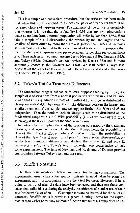
Sec. 3.3] Scheffé's S Statistic 45
This is a simple and convenient procedure, but the criticism has been madethat when this LSD is applied to all possible pairs of treatments there is anincreased chance of type-one errors. The argument of the critics is essentiallythat whereas it is true that the probability is 0.95 that any two observationsmade at random from a normal population will differ by less than 1.96a, if wetake a sample of n > 2 observations, the probability that the largest and thesmallest of them differ by more than 1.96a is greater than 0.05 and increasesas n increases. This has led to the development of tests with the property thatthe probability of a type-one error per experiment (rather than per comparison)is a. Three such tests in common use are due to Newman (1939), Duncan (1955),and Tukey (1953); Newman's test was revived by Keuls (1952) and is morecommonly known as the Newman-Keuls test. We shall derive Tukey's test.Accounts of the other two tests are found in the references cited and in the booksby Federer (1955) and Miller (1966).
3.2 Tukey's Test for Treatment Differences
The Studentized range is defined as follows. Suppose that x 1 , x2 , ... , xn is asample of n observations from a normal population with mean µ and variancea2 and that 5 2 is a quadratic estimate of a2 with 0 d.f., i.e., s 2/a2 is distributed aschi-square with 0 d.f. The range R(x) is the difference between the largest andsmallest members of the sample, and we suppose further that R(x) and s 2 areindependent. Then the random variable R(x)/s is said to be distributed as theStudentized range with 0 d.f. With probability (1 — a) we have R(x) < gn;ms,where qn;m is the upper a point of the Studentized range.
In Tukey's test we replace the x, of the previous paragraph by the treatmentmeans yi . and argue as follows. Under the null hypothesis, the probability is(1 — a) that R(y,.) < qt ms/^/r where 0 = N — t. Thus the probability is(j: — a) that Ti — Ti. < q^ ms/i/r for all pairs i, i'. We may therefore use q^ ms/-,/ras the least significant difference and declare that T t # Ti, if, and only if,IY{• — Yi'.1 > sgiN-t/\/r. Tukey's test is somewhat too conservative to suitsome experimenters. The tests of Newman and Keuls and of Duncan providecompromises between Tukey's test and the t test.
3.3 Scheffé's S Statistic
The three tests mentioned before are useful for testing comparisons. Theexperimenter usually has a few specific contrasts in mind when he plans hisexperiment, and it is appropriate to use the t test for these. However, if he isgoing to wait until after the data have been collected and then test those con-trasts that strike his eye during the analysis, the criticisms of blanket use of the ttest for the whole set of t(t — 1)/2 comparisons are no less valid for the set of allcontrasts. Scheffé's statistic provides a general hunting license for the experi-menter who wishes to test any estimable function that takes his fancy after he has
Dow
nloa
ded
12/1
1/12
to 1
29.1
28.2
07.2
42. R
edis
trib
utio
n su
bjec
t to
SIA
M li
cens
e or
cop
yrig
ht; s
ee h
ttp://
ww
w.s
iam
.org
/jour
nals
/ojs
a.ph
p
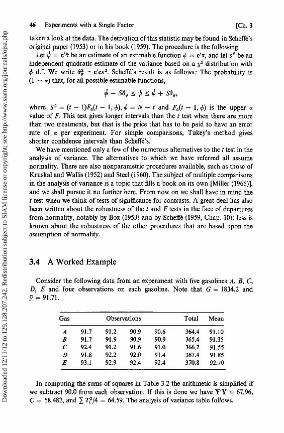
46 Experiments with a Single Factor [Ch. 3
taken a look at the data. The derivation of this statietic may be found in Scheffé'soriginal paper (1953) or in his book (1959). The procedure is the following.
Let = c'T be an estimate of an estimable function 0 = c'T, and let s 2 be anindependent quadratic estimate of the variance based on a X 2 distribution with0 d.f. We write & = c'cs 2 . Scheffé's result is as follows: The probability is(1 - a) that, for all possible estimable functions,
^-S& fr < +S&*,
where S 2 = (t - 1)Fa(t - 1, 0), 0 = N - t and Fa(t - 1, 0) is the upper «value of F. This test gives longer intervals than the t test when there are morethan two treatments, but that is the price that has to be paid to have an errorrate of a per experiment. For simple comparisons, Tukey's method givesshorter confidence intervals than Scheffé's.
We have mentioned only a few of the numerous alternatives to the t test in theanalysis of variance. The alternatives to which we have referred all assumenormality. There are also nonparametric procedures available, such as those ofKruskal and Wallis (1952) and Steel (1960). The subject of multiple comparisonsin the analysis of variance is a topic that fills a book on its own [Miller (1966)],and we shall pursue it no further here. From now on we shall have in mind thet test when we think of tests of significance for contrasts. A great deal has alsobeen written about the robustness of the t and F tests in the face of departuresfrom normality, notably by Box (1953) and by Scheffé (1959, Chap. 10); lens isknown about the robustness of the other procedures that are based upon theassumption of normality.
3.4 A Worked Example
Consider the following data from an experiment with five gasolines A, B, C,D, E and four observations on each gasoline. Note that G = 1834.2 andy = 91.71.
Gas Observations Total Mean
A 91.7 91.2 90.9 90.6 364.4 91.10B 91.7 91.9 90.9 90.9 365.4 91.35C 92.4 91.2 91.6 91.0 366.2 91.55D 91.8 92.2 92.0 91.4 367.4 91.85E 93.1 92.9 92.4 92.4 370.8 92.70
In computing the sums of squares in Table 3.2 the arithmetic is simplified ifwe subtract 90.0 from each observation. If this is done we have Y'Y = 67.96,C = 58.482, and 1 T,z/4 = 64.59. The analysis of variance table follows.D
ownl
oade
d 12
/11/
12 to
129
.128
.207
.242
. Red
istr
ibut
ion
subj
ect t
o SI
AM
lice
nse
or c
opyr
ight
; see
http
://w
ww
.sia
m.o
rg/jo
urna
ls/o
jsa.
php
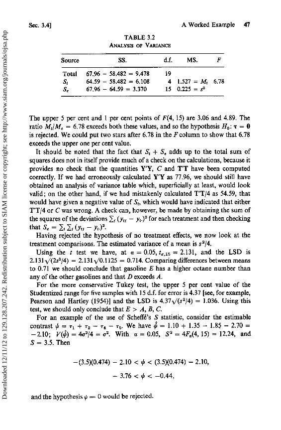
Sec. 3.4] A Worked Example 47
TABLE 3.2ANALYSIS OF VARIANCE
Source SS. d.f. MS. F
Total 67.96 — 58.482 = 9.478 19St 64.59 — 58.482 = 6.108 4 1.527 = Mt 6.78Se 67.96 — 64.59 = 3.370 15 0.225 = s 2
The upper 5 per cent and 1 per cent points of F(4, 15) are 3.06 and 4.89. Theratio Mt/Me = 6.78 exceeds both these values, and so the hypothesis Ho : r = 0is rejected. We could put two stars after 6.78 in the F column to show that 6.78exceeds the upper one per cent value.
It should be noted that the fact that S t + Se adds up to the total sum ofsquares does not in itself provide much of a check on the calculations, because itprovides no check that the quantities Y'Y, C and T'T have been computedcorrectly. If we had erroneously calculated Y'Y as 77.96, we should still haveobtained an analysis of variance table which, superficially at least, would lookvalid; on the other hand, if we had mistakenly calculated T'T/4 as 54.59, thatwould have given a negative value of St, which would have indicated that eitherT'T/4 or C was wrong. A check can, however, be made by obtaining the sum ofthe squares of the deviations Ij (yt5 — y,.)2 for each treatment and then checkingthat S. = 1 { Ij (yu —
Having rejected the hypothesis of no treatment effects, we now look at thetreatment comparisons. The estimated variance of a mean is s 2/4.
Using the t test we have, at a = 0.05, ta,15 = 2.131, and the LSD is2.131 //(2s2/4) = 2.131 x/0.1125 = 0.714. Comparing differences between meansto 0.71 we should conclude that gasoline E has a higher octane number thanany of the other gasolines and that D exceeds A.
For the more conservative Tukey test, the upper 5 per cent value of theStudentized range for five samples with 15 d.f. for error is 4.37 [see, for example,Pearson and Hartley (1954)] and the LSD is 4.37\/(S 2/4) = 1.036. Using thistest, we should only conclude that E> A, B, C.
For an example of the use of Scheffé's S statistic, consider the estimablecontrast 0=T 1 +'r2 —T4 —T5.We have +,i=1.10+1.35-1.85-2.70=—2.10; V(^i) = 4a2/4 = a2. With a = 0.05, S a = 4Fa(4, 15) = 12.24, andS = 3.5. Then
—(3.5)(0.474) — 2.10 < < (3.5)(0.474) — 2.10,
— 3.76 < 0 < —0.44,
and the hypothesis 0 = 0 would be rejected.Dow
nloa
ded
12/1
1/12
to 1
29.1
28.2
07.2
42. R
edis
trib
utio
n su
bjec
t to
SIA
M li
cens
e or
cop
yrig
ht; s
ee h
ttp://
ww
w.s
iam
.org
/jour
nals
/ojs
a.ph
p
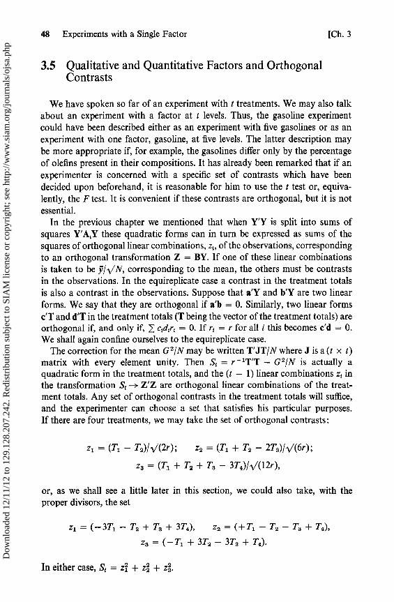
48 Experiments with a Single Factor [Ch. 3
3.5 Qualitative and Quantitative Factors and OrthogonalContrasts
We have spoken so far of an experiment with t treatments. We may also talkabout an experiment with a factor at t levels. Thus, the gasoline experimentcould have been described either as an experiment with five gasolines or as anexperiment with one factor, gasoline, at five levels. The Jatter description maybe more appropriate if, for example, the gasolines differ only by the percentageof olefins present in their compositions. It has already been remarked that if anexperimenter is concerned with a specific set of contrasts which have beendecided upon beforehand, it is reasonable for him to use the t test or, equiva-lently, the F test. It is convenient if these contrasts are orthogonal, but it is notessential.
In the previous chapter we mentioned that when Y'Y is split into sums ofsquares Y'A {Y these quadratic forms can in turn be expreseed as sums of thesquares of orthogonal linear combinations, z ti , of the observations, correspondingto an orthogonal transformation Z = BY. If one of these linear combinationsis taken to be y/^/N, corresponding to the mean, the others must be contrastsin the observations. In the equireplicate case a contrast in the treatment totalsis also a contrast in the observations. Suppose that a'Y and b'Y are two linearforms. We say that they are orthogonal if a'b = 0. Similarly, two linear formsc'T and d'T in the treatment totals (T being the vector of the treatment totals) areorthogonal if, and only if, r cid;r; = 0. If r• = r for all i this becomes c'd = 0.We shall again confine ourselves to the equireplicate case.
The correction for the mean G 2/N may be written T'JT/N where J is a (t x t)matrix with every element unity. Then St = r -1T'T — G 2/N is actually aquadratic form in the treatment totals, and the (t — 1) linear combinations z t inthe transformation St --> Z'Z are orthogonal linear combinations of the treat-ment totals. Any set of orthogonal contrasts in the treatment totals will suffice,and the experimenter can choose a set that satisfies his particular purposes.If there are four treatments, we may take the set of orthogonal contrasts:
zl = (T, — T2)/1/(2r); z2 = (Ti + T2 — 2T3)/1/(6r);
z3 = (T1 + T2 + T3 — 3T4)/\/( 12r),
or, as we shall see a little later in this section, we could also take, with theproper divisors, the set
zl = (— 3 T1 — T2 + T3 + 3T4), z2 = (+ Tl — T2 — T3 + T4),
z3 =(—T1 +3T2-3T3+T4).
In either case, St = zi + z + z3.
Dow
nloa
ded
12/1
1/12
to 1
29.1
28.2
07.2
42. R
edis
trib
utio
n su
bjec
t to
SIA
M li
cens
e or
cop
yrig
ht; s
ee h
ttp://
ww
w.s
iam
.org
/jour
nals
/ojs
a.ph
p
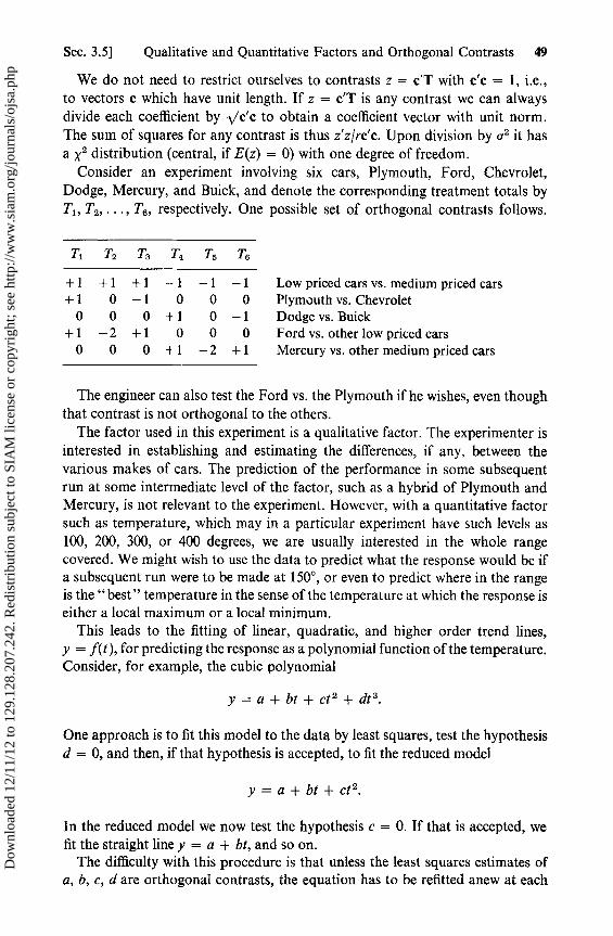
Sec. 3.5] Qualitative and Quantitative Factors and Orthogonal Contrasts 49
We do not need to restrict ourselves to contrasts z = c'T with c'c = 1, i.e.,to vectors c which have unit length. If z = c'T is any contrast we can alwaysdivide each coefficient by \/c'c to obtain a coefficient vector with unit norm.The sum of squares for any contrast is thus z'z/rc'c. Upon division by o2 it hasa X2 distribution (central, if E(z) = 0) with one degree of freedom.
Consider an experiment involving six cars, Plymouth, Ford, Chevrolet,Dodge, Mercury, and Buick, and denote the corresponding treatment totals byT1 , T2 ,. . ., T6, respectively. One possible set of orthogonal contrasts follows.
T1 Tz T3 T4 T5 Ts
+ 1 + 1 + 1 —1 —1 —1 Low priced cars vs. medium priced cars+ 1 0 —1 0 0 0 Plymouth vs. Chevrolet
0 0 0+ 1 0 —1 Dodge vs. Buick+ 1 —2 + 1 0 0 0 Ford vs. other low priced cars
0 0 0 + 1 —2 + 1 Mercury vs. other medium priced cars
The engineer can also test the Ford vs. the Plymouth if he wishes, even thoughthat contrast is not orthogonal to the others.
The factor used in this experiment is a qualitative factor. The experimenter isinterested in establishing and estimating the differences, if any, between thevarious makes of cars. The prediction of the performance in some subsequentrun at some intermediate level of the factor, such as a hybrid of Plymouth andMercury, is not relevant to the experiment. However, with a quantitative factorsuch as temperature, which may in a particular experiment have such levels as100, 200, 300, or 400 degrees, we are usually interested in the whole rangecovered. We might wish to use the data to predict what the response would be ifa subsequent run were to be made at 150°, or even to predict where in the rangeis the "best" temperature in the sense of the temperature at which the response iseither a local maximum or a local minimum.
This leads to the fitting of linear, quadratic, and higher order trend lines,y = f(t), for predicting the response as a polynomial function of the temperature.Consider, for example, the cubic polynomial
y = a + bt + ct 2 + dt 3 .
One approach is to fit this model to the data by least squares, test the hypothesisd = 0, and then, if that hypothesis is accepted, to fit the reduced model
y=a+bt+ct 2 .
In the reduced model we now test the hypothesis c = 0. If that is accepted, wefit the straight line y = a + bt, and so on.
The difficulty with this procedure is that unless the least squares estimates ofa, b, c, d are orthogonal contrasts, the equation has to be refitted anew at each
Dow
nloa
ded
12/1
1/12
to 1
29.1
28.2
07.2
42. R
edis
trib
utio
n su
bjec
t to
SIA
M li
cens
e or
cop
yrig
ht; s
ee h
ttp://
ww
w.s
iam
.org
/jour
nals
/ojs
a.ph
p
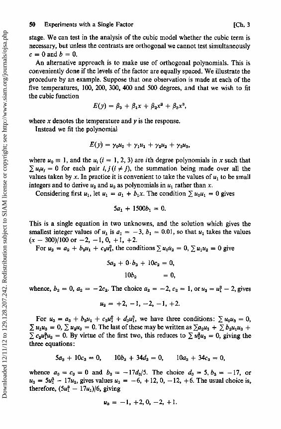
50 Experiments with a Single Factor [Ch. 3
stage. We can test in the analysis of the cubic model whether the cubic term isnecessary, but unless the contraets are orthogonal we cannot test simultaneouslyc = 0 and b = 0.
An alternative approach is to make use of orthogonal polynomials. This isconveniently done if the levels of the factor are equally spaced. We illustrate theprocedure by an example. Suppose that one observation is made at each of thefive temperatures, 100, 200, 300, 400 and 500 degrees, and that we wish to fitthe cubic function
E(y) = RO + Nlx + N2x2 + N3x3 ,
where x denotes the temperature and y is the response.Instead we fit the polynomial
E(y) = Youo + Y1u1 + Y2u2 + Y3u3,
where u0 = 1, and the ui (i = 1, 2, 3) are ith degree polynomials in x such that1 u,ui = 0 for each pair 1, j (i j), the summation being made over all thevalues taken by x. In practice it is convenient to take the values of u 1 to be smallintegers and to derive u 2 and u3 as polynomials in u 1 rather than x.
Considering first u 1 , let u1 = al + b lx. The condition uoul = 0 gives
5a1 + 1500b 1 = 0.
This is a single equation in two unknowns, and the solution which gives thesmallest integer values of u 1 is a1 = - 3, b l = 0.01, so that u1 takes the values(x - 300)/100 or -2, -1, 0, +1, +2.
For u2 = a2 + b2u1 + c2u1, the conditions uou2 = 0, 1 ulu2 = 0 give
5a2 + 0•b2 + 10c2 = 0,
10b2 = 0,
whence, b2 = 0, a2 = - 2c2. The choice a2 = - 2, c2 = 1, or u2 = u1 - 2, gives
u2 =+2,-1,-2,-1,+2.
For u3 = a3 + b3u1 + c3ui + d3ui, we have three conditions: uou3 = 0,u1u3 = 0, 1 u2u3 = 0. The last of these may be written as a2u3 + 1 b2ulu3 +
c2uiu3 = 0. By virtue of the first two, this reduces to uiu3 = 0, giving thethree equations:
5a3 + 10e3 = 0, 101,3 + 34d3 = 0, 10a3 + 34e3 = 0,
whence a3 = c3 = 0 and b3 = -17d3/5. The choice d3 = 5, b3 = - 17, oru3 = 5ui - 17u1 , gives values u3 = - 6, + 12, 0, -12, + 6. The usual choice is,therefore, (5ui - 17u1)/6, giving
u3 = - 1, +2,0, -2, +1.
Dow
nloa
ded
12/1
1/12
to 1
29.1
28.2
07.2
42. R
edis
trib
utio
n su
bjec
t to
SIA
M li
cens
e or
cop
yrig
ht; s
ee h
ttp://
ww
w.s
iam
.org
/jour
nals
/ojs
a.ph
p
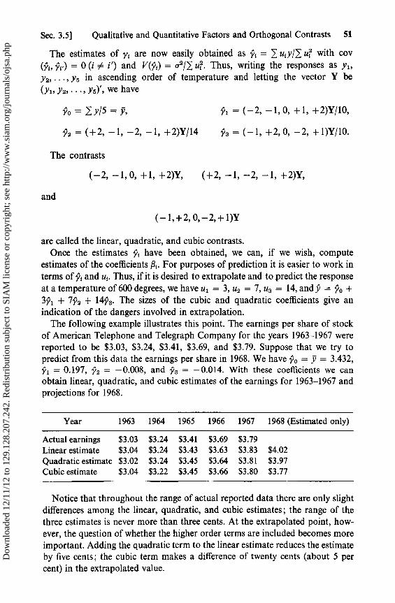
Sec. 3.5] Qualitative and Quantitative Factors and Orthogonal Contrasts 51
The estimates of y, are now easily obtained as yt = u, y/ ui with cov(y^, y{.) = 0 (i 0 i') and V( f) = a2/ ui'. Thus, writing the responses as y l ,Y2, ... , y5 in ascending order of temperature and letting the vector Y be(Y^, Y2, • • • , Ys)', we have
yo=1y15=y—, y1=(-2,-1,0,+1,+2)Y/10,
Y2 = (+2, —1, —2, —1, +2)Y/14 y3 = (-1, +2,0, —2, + 1)Y/10.
The contrasts
(-2, —1,0, +1, +2)Y, (+2, —1, —2, —1, +2)Y,
and
(-1,+2,0,-2,+1)Y
are called the linear, quadratic, and cubic contrasts.Once the estimates y i have been obtained, we can, if we wish, compute
estimates of the coefficients fl. For purposes of prediction it is easier to work interms of y, and u i . Thus, if it is desired to extrapolate and to predict the responseat a temperature of 600 degrees, we have u l = 3, u2 = 7, u3 = 14, and y = yo +321 + 722 + 1423 . The sizes of the cubic and quadratic coefficients give anindication of the dangers involved in extrapolation.
The following example illustrates this point. The earnings per share of stockof American Telephone and Telegraph Company for the years 1963-1967 werereported to be $3.03, $3.24, $3.41, $3.69, and $3.79. Suppose that we try topredict from this data the earnings per share in 1968. We have y o = y = 3.432,yl = 0.197, y2 = —0.008, and y3 = -0.014. With these coefficients we canobtain linear, quadratic, and cubic estimates of the earnings for 1963-1967 andprojections for 1968.
Year 1963 1964 1965 1966 1967 1968 (Estimated only)
Actual earnings $3.03 $3.24 $3.41 $3.69 $3.79
Linear estimate $3.04 $3.24 $3.43 $3.63 $3.83 $4.02Quadratic estimate $3.02 $3.24 $3.45 $3.64 $3.81 $3.97Cubic estimate $3.04 $3.22 $3.45 $3.66 $3.80 $3.77
Notice that throughout the range of actual reported data there are only slightdifferences among the linear, quadratic, and cubic estimates; the range of thethree estimates is never more than three cents. At the extrapolated point, how-ever, the question of whether the higher order terms are included becomes moreimportant. Adding the quadratic term to the linear estimate reduces the estimateby five cents; the cubic term makes a difference of twenty cents (about 5 percent) in the extrapolated value.
Dow
nloa
ded
12/1
1/12
to 1
29.1
28.2
07.2
42. R
edis
trib
utio
n su
bjec
t to
SIA
M li
cens
e or
cop
yrig
ht; s
ee h
ttp://
ww
w.s
iam
.org
/jour
nals
/ojs
a.ph
p

52 Experiments with a Single Factor [Ch. 3
3.6 The Gasoline Experiment (Continued)
Suppose now that the gasolines used in the experiment discussed Barlier inthis chapter differed only in the amount of some quantitative factor; in particular,suppose that gasolines A, B, C, D, and E were identical except that they con-tained x = 0, 1, 2, 3, 4 cubic centimeters, respectively, of some additive pergallon. We can subdivide St into linear, quadratic, cubic, and quartic com-ponents. The sum of squares for the linear contrast is
Sl = (-2T1 — T2 + T4 + 2T5)2/(10 x 4) = (14.8) 2/40 = 5.476;
the sums for the quadratic and cubic contrasts are
S2 = (2T1 — T2 — 2T3 — T4 + 2T5)2/(14 x 4) = (5.2) 2/56 = 0.483,
S3 = (—T1 + 2T2 — 2T4 + T5)2/(10 x 4) = (2.4)2/40 = 0.144.
The quartic contrast is (1, —4, 6, —4, 1)Y, and the corresponding sum ofsquares is (1.2)2/280 = 0.005.
These four sums of squares add up to St, which provides a check on ourcalculations. If the corresponding coefficient in the polynomial is zero, S,/s2 hasan F distribution with 1 and 15 d.f. The upper 5 per cent value of F(1, 15) is4.54. The only component that exceeds 4•54s 2 = 4.54(0.225) = 1.022 is S 1 . Weconclude that the higher order coefficients can be omitted from the polynomial.The estimated line is
Y=Yo+Yiui,
whereyo =y= 91.71, y 1 = 14.8/40 = 0.37, and u 1 = x — 2,ory=90.97+0.37x. The linear estimates and their deviations from the treatment means are
x 0 1 2 3 4
y, 90.97 91.34 91.71 92.08 92.45y,. — y, +0.13 +0.01 —0.16 —0.23 +0.25
We note that (y,. — Y,) = 0 and 4 (y,. — 9t)2 = 4(0.1580) = St — S,.
3.7 The Random Effects Model
In the previous model the levels of the factor were associated with unknownconstants T,. In the random effects model we have
yti=F^+at+e,1,
Dow
nloa
ded
12/1
1/12
to 1
29.1
28.2
07.2
42. R
edis
trib
utio
n su
bjec
t to
SIA
M li
cens
e or
cop
yrig
ht; s
ee h
ttp://
ww
w.s
iam
.org
/jour
nals
/ojs
a.ph
p
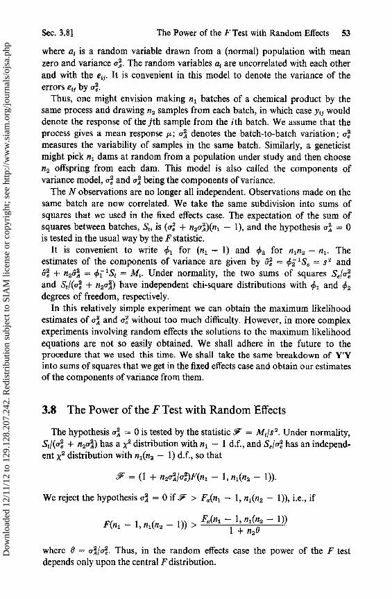
Sec. 3.8] The Power of the F Test with Random Effects 53
where a, is a random variable drawn from a (normal) population with meanzero and variance aÁ. The random variables a, are uncorrelated with each otherand with the eij . It is convenient in this model to denote the variance of theerrors et j by aé.
Thus, one might envision making n l batches of a chemical product by thesame process and drawing n2 samples from each batch, in which case yij woulddenote the response of the jth sample from the ith batch. We assume that theprocess gives a mean response µ; oÁ denotes the batch-to-batch variation; oémeasures the variability of samples in the same batch. Similarly, a geneticistmight pick n l dams at random from a population under study and then choosen2 offspring from each dam. This model is also called the components ofvariance model, aé and aÁ being the components of variance.
The N observations are no longer all independent. Observations made on thesame batch are now correlated. We take the same subdivision into sums ofsquares that we used in the fixed effects case. The expectation of the sum ofsquares between batches, St , is (c + n2aÁ)(n 1 — 1), and the hypothesis al = 0is tested in the usual way by the F statistic.
It is convenient to write q 1 for (n l — 1) and 02 for n 1n2 — n l. Theestimates of the components of variance are given by Qé = ¢2 1 Se = s 2 andQé + n2&Á = 'j 'S = M. Under normality, the two sums of squares Sefoéand St/(aé + n2aÁ) have independent chi-square distributions with ¢ 1 and 02
degrees of freedom, respectively.In this relatively simple experiment we can obtain the maximum likelihood
estimates of aA and aé without too much diffiiculty. However, in more complexexperiments involving random effects the solutions to the maximum likelihoodequations are not so easily obtained. We shall adhere in the future to theprocedure that we used this time. We shall take the same breakdown of Y'Yinto sums of squares that we get in the fixed effects case and obtain our estimatesof the components of variance from them.
3.8 The Power of the F Test with Random Effects
The hypothesis aÁ = 0 is tested by the statistic 9 = Mt/s 2 . Under normality,St/(ae + n2o) has a X2 distribution with n l — 1 d.f., and Se/Q has an independ-ent x2 distribution with n l(n2 — 1) d.f., so that
.F = (1 + n2a faé)F(nj — 1 , n1(n2 — 1 ))•
We reject the hypothesis oÁ = 0 if JF > Fa(nl — 1, n l(n2 — 1)), i.e., if
F(n l — 1, n l(n2 — 1)) > Fa(ni — 1, n1(n2 — 1 ))1 + n2 0
where 0 = a /oe. Thus, in the random effects case the power of the F testdepends only upon the tentral F distribution.
Dow
nloa
ded
12/1
1/12
to 1
29.1
28.2
07.2
42. R
edis
trib
utio
n su
bjec
t to
SIA
M li
cens
e or
cop
yrig
ht; s
ee h
ttp://
ww
w.s
iam
.org
/jour
nals
/ojs
a.ph
p

54 Experiments with a Single Factor [Ch. 3
EXAMPLE. Suppose that n l = 4, n2 = 6, 0 = 2.5, and that a is taken to be0.05. The upper 5 per cent value of F(3, 20) is 3.10. Then the power of the testis P[F(3, 20) > 3.10(1 + 6(2.5)) - '] = P[F(3, 20) > 0.19], which is approxi-mately 0.90.
3.9 Confidence Intervals for the Components of Variance
A confidence interval for oré can be obtained in the usual way using the X2distribution
[Se'Xu(42)] < ae < [+SeI XL(02)],
where for confidence, (1 — a), Xu, and XL are the upper and lower a/2 points ofthe chi-square distribution with 2 d.f.
An approximate confidence interval for aÁ can be obtained in the same wayusing St and assuming that 52 = o. We should then have
[St/Xu(ç61)] — s 2 < n2QA < [st/XL(ç61)] — s 2
Unfortunately, this method can give negative lower limits even when the F testrejects the hypothesis aÁ = 0. A preferable approach is to argue, as in theprevious section, that F/(1 + n 20) has a central F(o 1 , 02) distribution. Thenwe can obtain a confidence interval with confidence (1 — a) by writing
(1 + n20)FL < .F < (1 + n 2 0)FLI,
and manipulating it to obtain
n2 1(. /Fv — 1)s 2 < QA < n2 1(^/FL — 1)s 2 ,
where Fu and FL are the upper and lower a/2 points of F(O 1i 02). FL can beobtained from the usual tables by the identity Fl ,2 (q 1 , i2) = 1 /F«12(02, 0^)-
The general problem of confidence intervals for the components of variancehas been investigated by Bulmer (1957) and by Scheffé (1959). There are alsointeresting problems involving the allocation of observations. For a fixednumber N = n1n2 of observations, what is the best ratio nl /n2 for the experi-menter to take in designing his experiment? Should he perhaps choose anunbalanced design having unequal numbers of observations on the batches?For the case in which the same number of observations is made on each batch,the problem was solved by Hammersley (1949) [see also Scheffé (1959)].
3.10 The Gasoline Experiment (Continued)
Suppose that instead of being fixed effects the gasoline effects were random.Suppose that the gasolines were drawn from five different tanks, all filled with
Dow
nloa
ded
12/1
1/12
to 1
29.1
28.2
07.2
42. R
edis
trib
utio
n su
bjec
t to
SIA
M li
cens
e or
cop
yrig
ht; s
ee h
ttp://
ww
w.s
iam
.org
/jour
nals
/ojs
a.ph
p
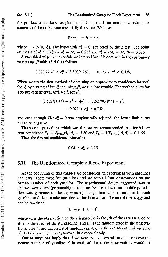
Sec. 3.11] The Randomized Complete Block Experiment 55
the product from the same plant, and that apart from random variation thecontents of the tanks were essentially the same. We have
Yu=i' +tt+ei3,
where tt — N(0, QÁ). The hypothesis QÁ = 0 is rejected by the F test. The pointestimates of oé and aÁ are 8é = Me = 0.225 and &Á = (Mt — Me)/4 = 0.326.
A two-sided 95 per cent confidence interval for aé is obtained in the customaryway using X2 with 15 d.f. as follows:
3.370/27.49 < aé < 3.370/6.262, 0.123 < aé < 0.538.
When we try the first method of obtaining an approximate confidence intervalfor a by putting s 2 for aé and using X2, we run into trouble. The method gives fora 95 per cent interval with 4 d.f. for Xa,
(1.527/11.14) — s 2 < 4oÁ < (1.527/0.4844) — s 2 ,
— 0.022 < aÁ < 0.732,
and even though Ho : oÁ = 0 was emphatically rejected, the lower limit turnsout to be negative.
The second procedure, which was the one we recommended, has for 95 percent confidence Fr, = F0025(4, 15) = 3.80 and FL = 1 /F0 025(15, 4) = 0.1155.
Then the desired confidence interval is
0.04<vÁ<3.25.
3.11 The Randomized Complete Block Experiment
At the beginning of this chapter we considered an experiment with gasolinesand cars. There were five gasolines and we wanted four observations on theoctane number of each gasoline. The experimental design suggested was tochoose twenty cars (presumably at random from whatever automobile popula-tion was germane to the experiment), assign four cars at random to eachgasoline, and then to take one observation in each car. The model then suggestedcan be rewritten
Yi=µ+ Ti +fr,
where yij is the observation on the ith gasoline in the jth of the cars assigned toit, T, is the effect of the ith gasoline, and ff is the random error in the observa-tions. The f i are uncorrelated random variables with zero means and varianceoÍ. Let us eiamine these f, f terms a little more closely.
Our assumptions imply that if we were to take several cars and observe theoctane number of gasoline A in each of them, the observations would be
Dow
nloa
ded
12/1
1/12
to 1
29.1
28.2
07.2
42. R
edis
trib
utio
n su
bjec
t to
SIA
M li
cens
e or
cop
yrig
ht; s
ee h
ttp://
ww
w.s
iam
.org
/jour
nals
/ojs
a.ph
p
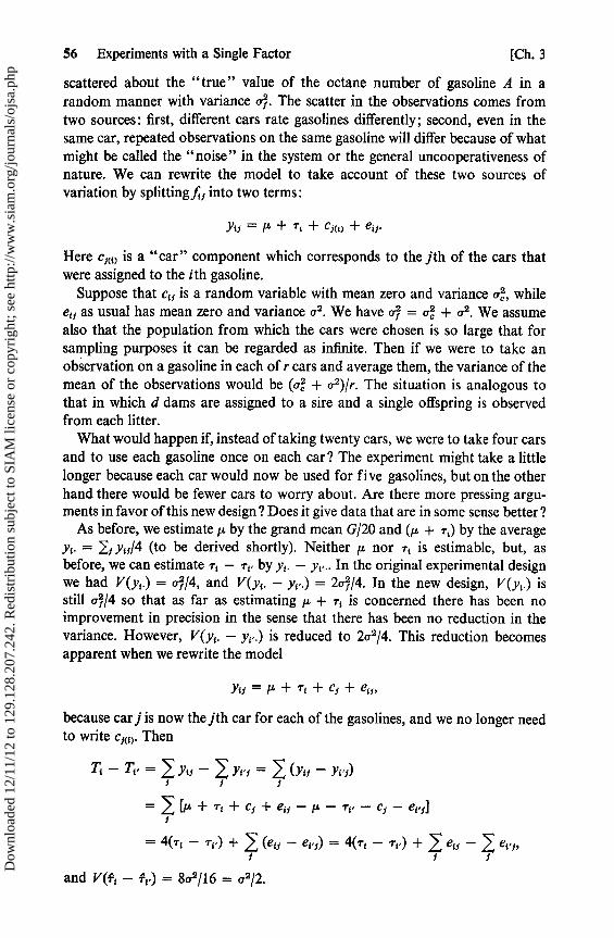
56 Experiments with a Single Factor [Ch. 3
scattered about the " t rue" value of the octane number of gasoline A in a random manner with variance a2. The scatter in the observations comes from two sources: first, different cars rate gasolines differently; second, even in the same car, repeated observations on the same gasoline will differ because of what might be called the "noise" in the system or the general uncooperativeness of nature. We can rewrite the model to take account of these two sources of variation by splitting ftj into two terms:
yu = I* + rt + cm + e^.
Here cm is a "car" component which corresponds to the^'th of the cars that were assigned to the ith gasoline.
Suppose that cw is a random variable with mean zero and variance a2, while etj as usual has mean zero and variance a2. We have a2 = a2 + a2. We assume also that the population from which the cars were chosen is so large that for sampling purposes it can be regarded as infinite. Then if we were to take an observation on a gasoline in each of r cars and average them, the variance of the mean of the observations would be (a2 + a2)jr. The situation is analogous to that in which d dams are assigned to a sire and a single offspring is observed from each litter.
What would happen if, instead of taking twenty cars, we were to take four cars and to use each gasoline once on each car? The experiment might take a little longer because each car would now be used for five gasolines, but on the other hand there would be fewer cars to worry about. Are there more pressing arguments in favor of this new design ? Does it give data that are in some sense better ?
As before, we estimate /* by the grand mean G/20 and (/n + T4) by the average yt- = 2 / W 4 (to be derived shortly). Neither /*. nor T, is estimable, but, as before, we can estimate T( — rf- by yt. — yv.. In the original experimental design we had V(yt.) = of/4, and V(yt. - yv.) = 2CT?-/4. In the new design, V(yt.) is still aj/4 so that as far as estimating p. + T( is concerned there has been no improvement in precision in the sense that there has been no reduction in the variance. However, V(y(. - yr.) is reduced to 2CT2/4. This reduction becomes apparent when we rewrite the model
yu = /* + T, + Cj + eu,
because car j is now they'th car for each of the gasolines, and we no longer need to write cm. Then
Ti - TV = 2 y» - 2 y*i = 2 ta> ~ yi'd
= 2 & + T( + ci + e« ~ V- - TY - Cj - eVj] i
= 4(n - T|.) + 2 («« - eVi) = 4(T, - T(.) + 2 ew ~ 2 *<'» i i i
and Vft - tt.) = 8<r2/16 = a2/2.
Dow
nloa
ded
12/1
1/12
to 1
29.1
28.2
07.2
42. R
edis
trib
utio
n su
bjec
t to
SIA
M li
cens
e or
cop
yrig
ht; s
ee h
ttp://
ww
w.s
iam
.org
/jour
nals
/ojs
a.ph
p
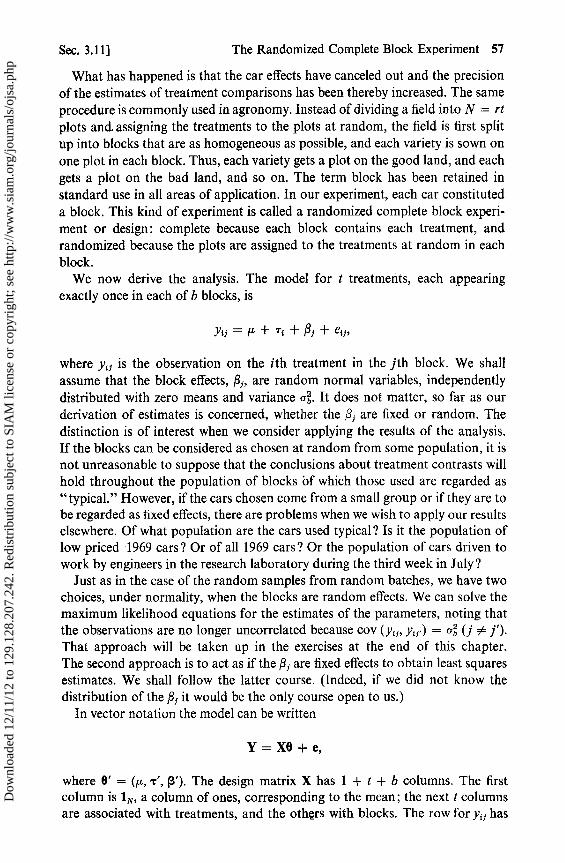
Sec. 3.11] The Randomized Complete Block Experiment 57
What has happened is that the car effects have canceled out and the precisionof the estimates of treatment comparisons has been thereby increased. The sameprocedure is commonly used in agronomy. Instead of dividing a field into N = rtplots and. assigning the treatments to the plots at random, the field is first splitup into blocks that are as homogeneous as possible, and each variety is sown onone plot in each block. Thus, each variety gets a plot on the good land, and eachgets a plot on the bad land, and so on. The term block has been retained instandard use in all areas of application. In our experiment, each car constituteda block. This kind of experiment is called a randomized complete block experi-ment or design: complete because each block contains each treatment, andrandomized because the plots are assigned to the treatments at random in eachblock.
We now derive the analysis. The model for t treatments, each appearingexactly once in each of b blocks, is
yt; =µ+T{ +Pf+e„,
where y { 3 is the observation on the ith treatment in the jth block. We shallassume that the block effects, fl, are random normal variables, independentlydistributed with zero means and variance ab. It does not matter, so far as ourderivation of estimates is concerned, whether the /3 are fixed or random. Thedistinction is of interest when we consider applying the results of the analysis.If the blocks can be considered as chosen at random from some population, it isnot unreasonable to suppose that the conclusions about treatment contrasts willhold throughout the population of blocks bf which those used are regarded as"typical.” However, if the cars chosen come from a small group or if they are tobe regarded as fixed effects, there are problems when we wish to apply our resultselsewhere. Of what population are the cars used typical? Is it the population oflow priced 1969 cars? Or of all 1969 cars? Or the population of cars driven towork by engineers in the research laboratory during the third week in July?
Just as in the case of the random samples from random batches, we have twochoices, under normality, when the blocks are random effects. We can solve themaximum likelihood equations for the estimates of the parameters, noting thatthe observations are no longer uncorrelated because cov (yij, yir.) = ab (j # j')That approach will be taken up in the exercises at the end of this chapter.The second approach is to act as if the / are fixed effects to obtain least squaresestimates. We shall follow the Jatter course. (Indeed, if we did not know thedistribution of the flf it would be the only course open to us.)
In vector notation the model can be written
Y = XO + e,
where 0' = (µ, r', (3'). The design matrix X has 1 + t + b columns. The firstcolumn is 1N, a column of ones, corresponding to the mean; the next t columnsare associated with treatments, and the oth§rs with blocks. The row for yj has
Dow
nloa
ded
12/1
1/12
to 1
29.1
28.2
07.2
42. R
edis
trib
utio
n su
bjec
t to
SIA
M li
cens
e or
cop
yrig
ht; s
ee h
ttp://
ww
w.s
iam
.org
/jour
nals
/ojs
a.ph
p
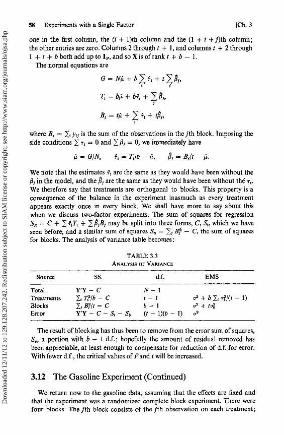
58 Experiments with a Single Factor [Ch. 3
one in the first column, the (i + l)th column and the (1 + t + j)th column;the other entries are zero. Columns 2 through t + 1, and columns t + 2 through1 + t + b both add up to 1N, and so X is of rank t + b — 1.
The oormal equations are
G=Nµ.+b f,+t>f,4 i
Ti =b11+bfj +^p1,
Bƒ =tµ+^ +{
where Bf = li yíj is the sum of the observations in the jth block. Imposing theside conditions 1 r, = 0 and 1 f f = 0, we immediately have
µ=G/N, Tt=Tilb—A, Pr =Bi/t—A.
We note that the estimates T, are the same as they would have been without the/3 in the model, and the nf are the same as they would have been without thé Ti .We therefore say that treatments are orthogonal to blocks. This property is aconsequence of the balance in the experiment inasmuch as every treatmentappears exactly once in every block. We shall have more to say about thiswhen we discuss two-factor experiments. The sum of squares for regressionSR = C + + 1 PA may be split into three forms, C, St , which we haveseen before, and a similar sum of squares S b = B — C, the sum of squaresfor blocks. The analysis of variante table becomes:
TABLE 3.3ANALYSIS OF VARIANCE
Source SS. d.f. EMS
Total Y'Y — C N-1Treatments Tz/b — C t — 1 o2 + b 1, T;/(t — 1)Blocks If B, /t — C b — 1 02 + tobError Y'Y — C — St — Sb (t — 1)(b — 1) a2
The result of blocking has thus been to remove from the error sum of squares,Se , a portion with b — 1 d.f.; hopefully the amount of residual removed hasbeen appreciable, at least enough to compensate for reduction of d.f. for error.With fewer d.f., the critical values of F and t will be increased.
3.12 The Gasoline Experiment (Continued)
We return now to the gasoline data, assuming that the effects are fixed andthat the experiment was a randomized complete block experiment. There werefour blocks. The jth block consists of the jth observation on each treatment;
Dow
nloa
ded
12/1
1/12
to 1
29.1
28.2
07.2
42. R
edis
trib
utio
n su
bjec
t to
SIA
M li
cens
e or
cop
yrig
ht; s
ee h
ttp://
ww
w.s
iam
.org
/jour
nals
/ojs
a.ph
p
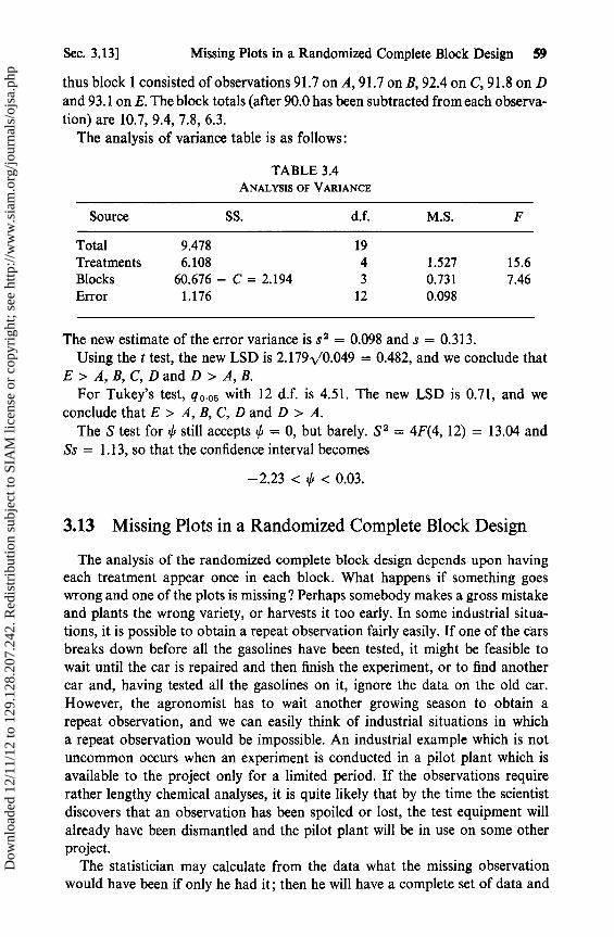
Sec. 3.13] Missing Plots in a Randomized Complete Block Design 59
thus block 1 consisted of observations 91.7 on A, 91.7 on B, 92.4 on C, 91.8 on Dand 93.1 on E. The block totals (after 90.0 has been subtracted from each observa-tion) are 10.7, 9.4, 7.8, 6.3.
The analysis of variance table is as follows:
TABLE 3.4ANALYSIS OF VARIANCE
Source SS. d.f. M.S. F
Total 9.478 19Treatments 6.108 4 1.527 15.6Blocks 60.676 — C = 2.194 3 0.731 7.46Error 1.176 12 0.098
The new estimate of the error variance is 52 = 0.098 and s = 0.313.
Using the t test, the new LSD is 2.179V0.049 = 0.482, and we conclude thatE> A,B,C,DandD > A,B.
For Tukey's test, go.05 with 12 d.f. is 4.51. The new LSD is 0.71, and weconclude that E> A, B, C, D and D > A.
The S test for 0 still accepts 0 = 0, but barely. SZ = 4F(4, 12) = 13.04 andSs = 1.13, so that the confidence interval becomes
—2.23<0<0.03.
3.13 Missing Plots in a Randomized Complete Block Design
The analysis of the randomized complete block design depends upon havingeach treatment appear once in each block. What happens if something goeswrong and one of the plots is missing? Perhaps somebody makes a gross mistakeand plants the wrong variety, or harvests it too early. In some industrial situa-tions, it is possible to obtain a repeat observation fairly easily. If one of the carsbreaks down before all the gasolines have been tested, it might be feasible towait until the car is repaired and then finish the experiment, or to find anothercar and, having tested all the gasolines on it, ignore the data on the old car.However, the agronomist has to wait another growing season to obtain arepeat observation, and we can easily think of industrial situations in whicha repeat observation would be impossible. An industrial example which is notuncommon occurs when an experiment is conducted in a pilot plant which isavailable to the project only for a limited period. If the observations requirerather lengthy chemical analyses, it is quite likely that by the time the scientistdiscovers that an observation has been spoiled or lost, the test equipment willalready have been dismantled and the pilot plant will be in use on some otherproject.
The statistician may calculate from the data what the missing observationwould have been if only he had it; then he will have a complete set of data and
Dow
nloa
ded
12/1
1/12
to 1
29.1
28.2
07.2
42. R
edis
trib
utio
n su
bjec
t to
SIA
M li
cens
e or
cop
yrig
ht; s
ee h
ttp://
ww
w.s
iam
.org
/jour
nals
/ojs
a.ph
p
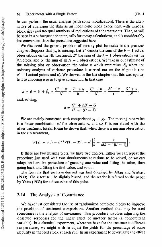
60 Experiments with a Single Factor [Ch. 3
he can perform the usual analysis (with some modification). There is the alter-native of analyzing the data as an incomplete block experiment with unequalblock Bizes and unequal numbers of replications of the treatments. That, as willbe seen in a subsequent chapter, calls for messy calculations, and is considerablyless convenient than the procedure suggested here.
We discussed the general problem of missing plot formulae in the previouschapter. Suppose that y jj is missing. Let T' denote the sum of the b — 1 actualobservations on the ith treatment, B' the sum of the t — 1 observations on thejth block, and G' the sum of all N — 1 observations. We take as our estimate ofthe missing plot or observation the value u which minimizes S e when theordinary analysis of variance procedure is carried out on the N points (theN — 1 actual points and u). We showed in the last chapter that this was equiva-lent to choosing u so as to give an exact fit. In that case
G'+u T'+u G'+u B' +u G'+uu=µ+T,+flf = N + b N + t — N
and, solving,
_ tT' +bB' —Gu (b — 1)(t — 1)
We are mainly concerned with comparisons y,. — y,... The missing plot valueis a linear combination of the observations, and so Ti is correlated with theother treatment totals. It can be shown that, when there is a missing observationin the ith treatment,
V(yi .—yt-.)=b-2V(T,—T;.)=a2lb+b(b— 1)(t — 1)]
If there are two missing plots, we have two choices. Either we can repeat theprocedure just used with two simultaneous equations to be solved, or we canadopt an iterative procedure of guessing one value and fitting the other, thengoing back and fitting the first value, and so on.
The formula that we have derived was first obtained by Allan and Wishart(1930). The F test will be slightly biased, and the reader is referred to the paperby Yates (1933) for a discussion of this point.
3.14 The Analysis of Covariance
We have just considered the use of randomized complete blocks to improvethe precision of treatment comparisons. Another method that may be usedsometimes is the analysis of covariance. This procedure involves adjusting theobserved responses for the linear effect of another factor (a concomitantvariable). In a chemical experiment, where we have for the treatments differenttemperatures, we might wish to adjust the yields for the percentage of someimpurity in the feed stock at each run. In an experiment to investigate the effect
Dow
nloa
ded
12/1
1/12
to 1
29.1
28.2
07.2
42. R
edis
trib
utio
n su
bjec
t to
SIA
M li
cens
e or
cop
yrig
ht; s
ee h
ttp://
ww
w.s
iam
.org
/jour
nals
/ojs
a.ph
p
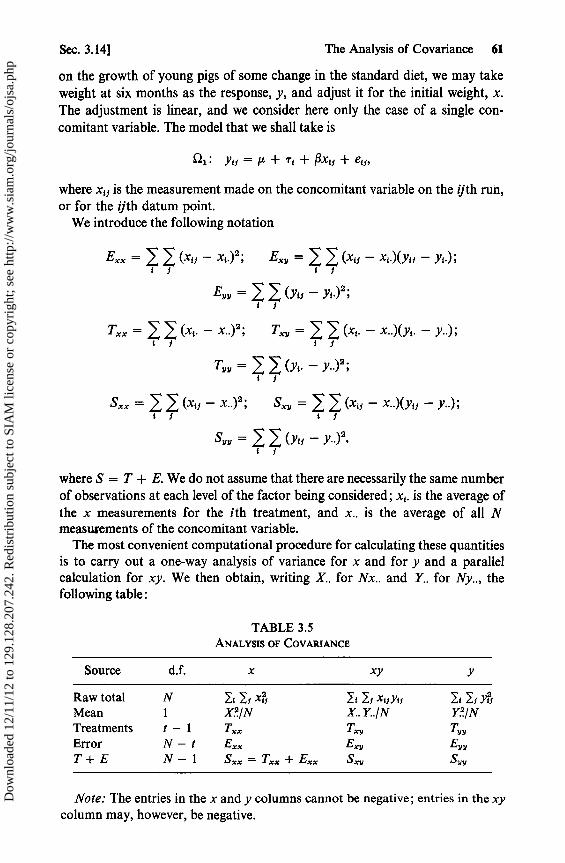
Sec. 3.14] The Analysis of Covariance 61
on the growth of young pigs of some change in the standard diet, we may takeweight at six months as the response, y, and adjust it for the initial weight, x.The adjustment is linear, and we consider here only the case of a single con-comitant variable. The model that we shall take is
f: Yti = F^ + Ti + 1xt7 + eti,
where x15 is the measurement made on the concomitant variable on the ijth run,or for the ijth datum point.
We introduce the following notation
E„. = (x{i — xt•)2 ; E., = (xt1 — x.)(Yt, — Yt•);t r t f
E, . = (Yu — yt.)2 ;t i
T, = (x,. — x..)2 ; Txv = G (xt . — x..)(Yt. —
T vv = (yt. —y..)2 ;t r
S, = (x,i — x..)2 ; S.. = (x1, — x..)(Yts — Y..);
S» = G > (Ytt — y•) 2.{ r
where S = T + E. We do not assume that there are necessarily the same numberof observations at each level of the factor being considered; x t. is the average ofthe x measurements for the i th treatment, and x.. is the average of all Nmeasurements of the concomitant variable.
The most convenient computational procedure for calculating these quantitiesis to carry out a one-way analysis of variance for x and for y and a parallelcalculation for xy. We then obtain, writing X.. for Nx.. and Y.. for Ny.., thefollowing table:
TABLE 3.5ANALYSIS OF COVARIANCE
Source d.f. x xy y
Raw total N 1, J i 4 l s Iƒ x,5Yi l i l t Y%Mean 1 X^/N X..Y../N Y.^/NTreatments t — 1 T. T., T.Error N — t Exx Exy Ey„
T + E N — 1 S...=T...+Exx. Sz7 Sw
No te: The entries in the x and y columns cannot be negative; entries in the xy
column may, however, be negative.
Dow
nloa
ded
12/1
1/12
to 1
29.1
28.2
07.2
42. R
edis
trib
utio
n su
bjec
t to
SIA
M li
cens
e or
cop
yrig
ht; s
ee h
ttp://
ww
w.s
iam
.org
/jour
nals
/ojs
a.ph
p

62 Experiments with a Single Factor [Ch. 3
We can now proceed in two ways, and it is constructive to consider both.When we introduce blocks, we shall set up and solve the normal equations. Atthis time we shall use the other approach.
Suppose that we have no treatment effects. Our model would be
Oo: yit=ii+Pxit+eit.
Under this model P is estimated by = S./Sxz, and the sum of squares forerror is Sé = S, — (S)2/S.
Suppose now that we have treatment effects and that the model is 0 1 . Thismodel implies that there is a family of parallel lines, one for each treatment.Some of the lines may coincide; S2o corresponds to the case in which all ofthe lines coincide. The data for the ith treatment alone give an estimate bi of ,where
=
I f (xif — xi.)(Yif — Yi.)Qs
b` 1i (xi5 — xi.)2
and V(bi) = (xi> — xi .)2
The several estimates, bi, are clearly uncorrelated because they involve differentdata. The minimum variance unbiased combined estimate from them is P =li wibi, where the weight, wi, given to any bi is inversely proportional to V(bs),and wi = 1. This gives w, = Ii (x 5 — xt.)2IE.„ and
p = Ex /E x .
The ith line is thus yi, = y,. + P(xiJ — xi .).The sum of the squares of the deviations about the several lines is
Se = (Yi — yi• — P(xii — xi•))2 = E — (E.v) 2/E .t 1
We can now write down the analysis of variance table. The sum of squaresfor treatments is the reduction in error made by fitting individual Tines ratherthan a common line, i.e., SB — Se .
TABLE 3.6ANALYSIS OF VARIANCE
Source d.f. SS
Total N — 1 S.Fitting a single line 1 (S.Y)2/Sxx
Treatments t — 1 (Sy, — (SS„)2/Sxz) — (E (Exy)2/Exx)
Error N — t — 1 Ey, — (E.xy)2/Ezx
The error variance, o2, is estimated by S 2 = (N — t — 1) - '(E22 — (Ex )2/Exx)•
Dow
nloa
ded
12/1
1/12
to 1
29.1
28.2
07.2
42. R
edis
trib
utio
n su
bjec
t to
SIA
M li
cens
e or
cop
yrig
ht; s
ee h
ttp://
ww
w.s
iam
.org
/jour
nals
/ojs
a.ph
p
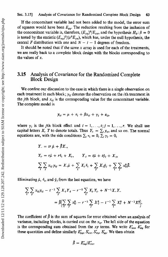
Sec. 3.15] Analysis of Covariance for Randomized Complete Block Design 63
If the concomitant variable had not been added to the model, the error sumof squares would have been E^ v . The reduction resulting from the inclusion ofthe concomitant variable is, therefore, (E„„)2IExx, and the hypothesis Ha : S = 0is tested by the statistic (Ex„)2/(s2Exx), which has, under the null hypothesis, thecentral F distribution with one and N — t — 1 degrees of freedom.
It should be noted that if the same x array is used for each of the treatments,we are really back to a complete block design with the blocks corresponding tothe values of x.
3.15 Analysis of Covariance for the Randomized CompleteBlock Design
We confine our discussion to the case in which there is a single observation oneach treatment in each block; y t, denotes the observation on the ith treatment inthe jth block, and x,f is the corresponding value for the concomitant variable.The complete model is
ytf =g+ r +jxtf+yj+eti,
where y, is the jth block effect and i = 1, ..., t; j = 1, ..., r. We shall usecapital letters X, Y to denote totals. Thus Y{ . = y, and so on. The normaiequations are, with the side conditions = 0, If yf = 0,
Y..= tri +px..,
Yt . = rµ + rTt + Xt ., Y., = tµ + ty, + X.,,
xtiyu = X..µ + ^ Xt •Tt + ^ XrYr +11 t i t i
Eliminating µ, T,, and y, from the last equation, we have
xuyti — t 1 > X.1 Y.5 — r' X. YY . + N -1 X.. Y..t i i t
_ {^ ^ xti — r —1 X.1 — t —1 X a + N —1 X }.
The coefficient of P is the sum of squares for error obtained when an analysis ofvariance, including blocks, is carried out on the x,5. The left side of the equationis the corresponding sum obtained from the xy terms. We write Exx, Ezj forthese quantities and define similarly E^, Sxx, Sx v, S. We then obtain
xv xx•
Dow
nloa
ded
12/1
1/12
to 1
29.1
28.2
07.2
42. R
edis
trib
utio
n su
bjec
t to
SIA
M li
cens
e or
cop
yrig
ht; s
ee h
ttp://
ww
w.s
iam
.org
/jour
nals
/ojs
a.ph
p
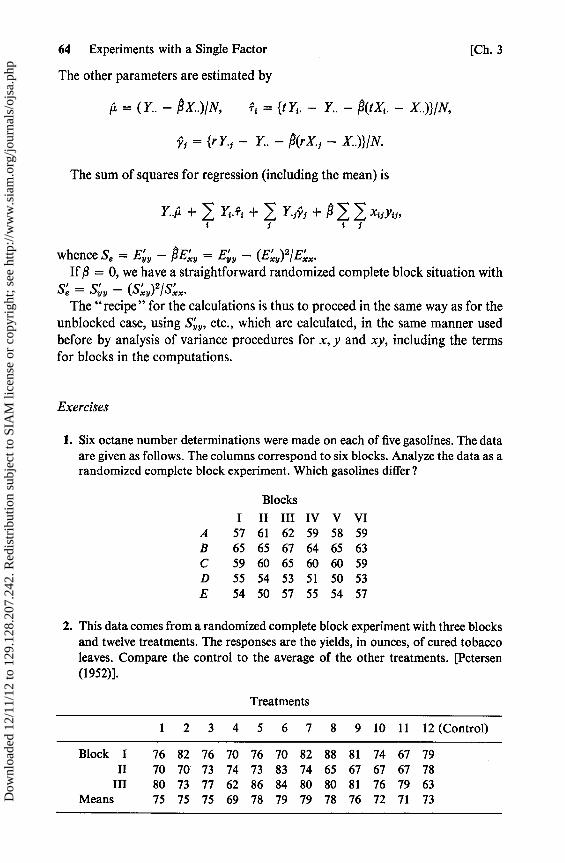
64 Experiments with a Single Factor [Ch. 3
The other parameters are estimated by
µ = (Y.. — $X..)/N, T, = {t Y{. — Y.. — P(tX{. — X..)}IN,
y1 = {r Y., — Y.. — P(rX. j — X..)}IN.
The sum of squares for regression (including the mean) is
Y..µ + YY .Ti + Y., 1 +
whence Se = Eyy — PEx, = E^„ — (Exy)ZI Eax•If P = 0, we have a straightforward randomized complete block situation with
Se = S ' . — (Sxy) ZI Sxx•
The "recipe" for the calculations is thus to proceed in the same way as for theunblocked case, using S, ,, etc., which are calculated, in the same manner usedbefore by analysis of variance procedures for x, y and xy, including the termsfor blocks in the computations.
Exercises
1. Six octane number determinations were made on each of five gasolines. The dataare given as follows. The columns correspond to six blocks. Analyze the data as arandomized complete block experiment. Which gasolines differ?
Blocks
I II III IV V VIA 57 61 62 59 58 59
B 65 65 67 64 65 63
C 59 60 65 60 60 59D 55 54 53 51 50 53
E 54 50 57 55 54 57
2. This data comes from a randomized complete block experiment with three blocksand twelve treatments. The responses are the yields, in ounces, of cured tobaccoleaves. Compare the control to the average of the other treatments. [Petersen(1952)].
Treatments
1 2 3 4 5 6 7 8 9 10 11 12 (Control)
Block I 76 82 76 70 76 70 82 88 81 74 67 79II 70 70 73 74 73 83 74 65 67 67 67 78
III 80 73 77 62 86 84 80 80 81 76 79 63Means 75 75 75 69 78 79 79 78 76 72 71 73D
ownl
oade
d 12
/11/
12 to
129
.128
.207
.242
. Red
istr
ibut
ion
subj
ect t
o SI
AM
lice
nse
or c
opyr
ight
; see
http
://w
ww
.sia
m.o
rg/jo
urna
ls/o
jsa.
php

Exercises 65
3. An experiment is to be designed to compare t new treatments with a controltreatment. A one-way layout is to be used; there are to be ro observations on thecontrol and r observations on each of the new treatments. Show that for any givenvalue of N the variante of the comparisons between the control treatment andthe new treatments, V(T0 - T{), is minimized if ro = rVt.
4. Let x take the values 1, 2, 3,..., n, and let y = x2. Show that the correlationcoefficient of x and y is given by
15(n + 1)2r2= 16n2 + 30n + 11'
which is a monotone decreasing function of n with limit 15/16.5. Two observations are made at x = 0 and one each at x = 1, 2, 3, and 4. Find a
set of orthogonal linear, quadratic polynomials.6. If x takes the values 1, 2,..., n once each, show that the polynomials u1 = x
— z, u2 = 12u1 — (na — 1) are orthogonal.7. Find a pair of orthogonal linear and quadratic polynomials when x takes the
values 0, 1, 2, 4, 8.8. Find the expected value of St for a randomized complete block design when one
of the plots is missing and its value has been calculated by the formula.9. Derive the formula for V(yh — yt) if one of the observations on the hth treatment
has been calculated by the missing plot formula.10. Find the expected value of Se in the random effects case when there are r, observa-
tions on the ith variety and the r, are not all equal.11. In the random effects model for the one-way layout with r observations on each
variety, use the method of maximum liklihood under the normality assumption toobtain estimates of oé and oa,, and to test the hypothesis H0 : QÁ = 0.
12. Assume that in a randomized complete block experiment the errors e iƒ and theblock effects S, are normal random variables. Use the method of maximumlikelihood to derive estimates of r and a.
13. Prove that St and Se are independent in the random effects model under normalityin the balanced case. Is it true even when there are unequal numbers of observa-tions on the varieties?
14. Suppose that in a randomized complete block design the observation on the firsttreatment in the first block and the observation on the second treatment in thesecond block are missing. Obtain formulae for calculating the two missingvalues.
15. Repeat problem 14 for the case in which the two missing plots are in the sameblock.
16. Scheffé (1959, p. 70) points out that the F test will reject Ho if, and only if,there is at least one estimable y which has a significant estimate by his S test.Is it true that if, in the fixed effects case, the F ratio is significant, then there is atleast one contrast that will be declared significantly different from zero by thet test? Is the converse true? If not, give an example.
Dow
nloa
ded
12/1
1/12
to 1
29.1
28.2
07.2
42. R
edis
trib
utio
n su
bjec
t to
SIA
M li
cens
e or
cop
yrig
ht; s
ee h
ttp://
ww
w.s
iam
.org
/jour
nals
/ojs
a.ph
p

CHAPTER 4
Experimentswith
Two Factors
In the previous chapter we considered as an example of a randomized blockexperiment an experiment in which t treatments (gasolines) were tested in r cars.The cars were chosen at random from some appropriate population and theyconstituted the blocks of the design. The purpose of the blocking was to improvethe precision of the comparisons between gasolines. The differences betweencars were eliminated in estimating the gasoline contrasts. In some presentationsthe analysis of variance tables contain under the heading, "Expected meansquare for the sum of squares between blocks," the single word discard. Thevariation between blocks is considered as something to be "backed out" of theexperimental analysis.
Suppose, however, that instead of having r nondescript vehicles, we had beenat pains to choose a Chevrolet, a Plymouth, a Ford, and so on, with the resultthat cars could be considered as a second factor occurring at r levels. The twofactors are said to be crossed. Each factor appears at least once with each levelof the other factor. Indeed, each gasoline sees each car exactly once, and eachcar sees each gasoline exactly once. How, if at all, does this experiment differfrom the randomized block experiment of the previous chapter? We considerfirst the simple experiment in which each gasoline is tested only once in each car.This experimental setup is called the two-way layout (or two-way crossedclassification) with one observation per cell.
4.1 The Two-Way Layout with One Observation per Cell
We shall find it convenient now to think about a factorial experiment involvingtwo factors, A and B, with a and b levels respectively. In our previous example,the factors were gasolines and cars. The factors can be qualitative or quantitative.
ri
Dow
nloa
ded
12/1
1/12
to 1
29.1
28.2
07.2
42. R
edis
trib
utio
n su
bjec
t to
SIA
M li
cens
e or
cop
yrig
ht; s
ee h
ttp://
ww
w.s
iam
.org
/jour
nals
/ojs
a.ph
p

Sec. 4.1] The Two-Way Layout with One Observation per Cell 67
The levels of the car factor could be Plymouth, Ford, etc.; the levels of thegasoline factor might be one ml/gal, 2 ml/gal, etc., of some additive like lead.Our model is the simple additive model Y = XO + e, or
yi=µ+ at+ilj +et1,
where y{1 is the observation made on (or the response at) the ith level of A andthe jth level of B, and et, is the random error with the usual assumptions. Theother terms in the model are unknown constante; µ represents a grand mean, a, isthe main effect of the i th level of A, and f is the main effect of the j th level of B.
The design matrix X has N = ab rows and 1 + a + b columns. The rowcorresponding to the observation y ij has unit elements in the first, the (i + 1)thand the (1 + a + j)th columns, and zeros elsewhere. The first column is 1 N •The sum of the next a columns is also 1N , and the sum of the last b columns isalso 1N ; it follows that r(X) < a + b — 1. This implies that we have twoparameters too many. We could get rid of one parameter by putting µ = 0,which is the same as leaving µ out of the model, but we would still be faced with asingular matrix X'X. The most common procedure is to leave µ in the model andto impose the two side conditions 1'a = 0 and 1'(3 = 0, where a and p are theveetors of the main effects a{ and Pi . The parameters µ, a,, and / are not estim-able. The expected values of observations, contrasts in the parameters a,, andcontrasts in the f, are estimable.
As far as the derivation of the rums of squares is concerned, there is no changefrom the randomized complete block design. We write T i. = y 1 = byt . andT 1 = l ; yi; = ay.f. Then % = y, «, = y,. — y and P1 = y. ; — y. Writing a. fori, aja and P. for I; fj/b, we have
E(ái) = µ + ai + P. — µ — a. — P. = ai — a..
This brings out the concept of the main effect of the ith level of A as the differ-ence between the average response at the i th level of A and the average responseat all levels of A.
The comparison a• — a ;. is estimated by y i . — y; ... We point out again thatjust as was the case in the randomized block experiment, the B effects arecanceled out in the expectation of the contrast because of the balance, ororthogonality, that was built into the experiment by having each level of Aappear exactly once with each level of B. Similarly, the comparison fj — /1. isestimated by y. j — y.j-. Table 4.1 follows:
TABLE 4.1ANALYSIS OF VARIANCE
Source SS d.f.
Total 1, J f y? — G 2/N ab — 1Between levels of A Tlb — G 2/N a — 1Between levels of B JJ T.fla — G 2/N b — 1Residual 1, Ij y, — 7-, T,?/b — J t T.J/a + G 2/N (a — 1)(b — 1)
Dow
nloa
ded
12/1
1/12
to 1
29.1
28.2
07.2
42. R
edis
trib
utio
n su
bjec
t to
SIA
M li
cens
e or
cop
yrig
ht; s
ee h
ttp://
ww
w.s
iam
.org
/jour
nals
/ojs
a.ph
p

68 Experiments with Two Factors [Ch. 4
Tests of hypotheses about the a{ and about the /3 are carried out just as in arandomized complete block design.
EXAMPLE. In their studies on the habits of Zebu cattle, Rollison et al.observed a group of cattle and recorded every minute which of the cattle weregrazing. The same group of five observcrs was used throughout the work carriedout at Entebbe, Uganda. The authors (1956) reported upon an experiment carriedout to compare these observers. They watched a group of ten cattle in the samepaddock for eighty-eight minutes one afternoon. The numbers recorded are thenumbers of minutes in which observer i reported that he saw animal j grazing.
Observers Animals
1 2 3A 34 76 75B 33 76 72C 35 78 76D 34 77 71E 33 77 70
Total 169 384 364
4 5 6 7 8 9 10 Total31 61 82 82 67 72 38 61829 60 82 84 67 72 36 61130 65 86 88 66 76 37 63729 60 78 83 67 72 37 60827 59 81 82 67 70 33 599
146 305 409 419 334 362 181 3073
TABLE 4.2ANALYSIS OF VARIANCE
Source d.f. MS
Animals 9 2149.42Observers 4 20.33Residual 36 2.06Total 49
4.2 Orthogonality with More Than One Observation per Cell
Suppose that we relax the requirement that there be exactly one observation ateach level of A and at each level of B, and allow several observations. The modelremains the same, except that we could write yU,„ to denote the mth observationat the ith level of A and the jth level of B, i.e., in the (ij)th cell. If there are anequal number of observations in each cell, the analysis will be a trivial extensionof that of the previous section. If the cell numbers are not all the same, thesolution of the normai equations is complicated by the fact that we cannot findtwo side conditions that will separate the unknowns in a simple fashion.
We are not going to discuss the solution of the equations at this time. We havealready spoken in Chapter 2 about methods of finding pseudo-inverses, and thematter will come up again in more detail in our discussion of incomplete block
Dow
nloa
ded
12/1
1/12
to 1
29.1
28.2
07.2
42. R
edis
trib
utio
n su
bjec
t to
SIA
M li
cens
e or
cop
yrig
ht; s
ee h
ttp://
ww
w.s
iam
.org
/jour
nals
/ojs
a.ph
p
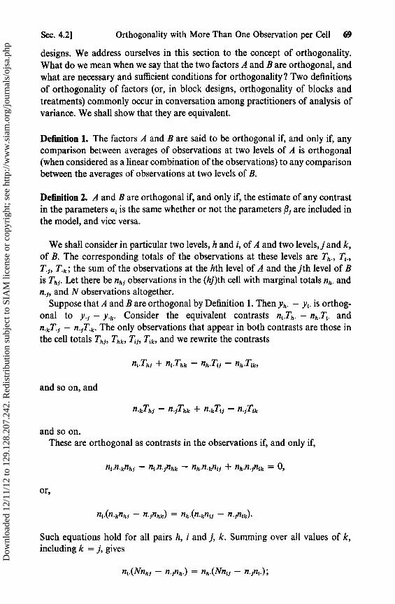
Sec. 4.2] Orthogonality with More Than One Observation per Cell 69
designs. We address ourselves in this section to the concept of orthogonality.What do we mean when we say that the two factors A and B are orthogonal, andwhat are necessary and sufficient conditions for orthogonality? Two definitionsof orthogonality of factors (or, in block designs, orthogonality of blocks andtreatments) commonly occur in conversation among practitioners of analysis ofvariance. We shall show that they are equivalent.
Definition 1. The factors A and B are said to be orthogonal if, and only if, anycomparison between averages of observations at two levels of A is orthogonal(when considered as a linear combination of the observations) to any comparisonbetween the averages of observations at two levels of B.
Definition 2. A and B are orthogonal if, and only if, the estimate of any contrastin the parameters a i is the same whether or not the parameters /3 are included inthe model, and vice versa.
We shall consider in particular two levels, h and i, of A and two levels, j and k,of B. The corresponding totals of the observations at these levels are T h ., T,.,T.1, T.k ; the sum of the observations at the hth level of A and the jth level of Bis Thf . Let there be n,^5 observations in the (hj)th cell with marginal totals n,^. andn.5, and N observations altogether.
Suppose that A and B are orthogonal by Definition 1. Then yh . — yi . is orthog-onal to y., — y.k. Consider the equivalent contrasts n { .Th . — nh.T{. andn.kT.j — n. IT. k. The only observations that appear in both contrasts are those inthe cell totals Thj, Thk, T,j, Tik, and we rewrite the contrasts
n{.Thj + ni .Thk — nh.Tlj — nh.Tik,
and so on, and
n.kThi — n. jThk + n.kTl j — n.lT{k
and so on.These are orthogonal as contrasts in the observations if, and only if,
n { •n• knhf — n i .n. jnhk — nh •n.knt1 + nh .n.1nik = 0,
or,
n{.(n.knhj — n.inhk) = n h .(n. kn ij — n.jnik).
Such equations hold for all pairs h, i and j, k. Summing over all values of k,including k = j, gives
nt .(Nnh1 — n.Jnh.) = nh .(Nnti — n.jni.);
Dow
nloa
ded
12/1
1/12
to 1
29.1
28.2
07.2
42. R
edis
trib
utio
n su
bjec
t to
SIA
M li
cens
e or
cop
yrig
ht; s
ee h
ttp://
ww
w.s
iam
.org
/jour
nals
/ojs
a.ph
p

70 Experiments with Two Factors [Ch. 4
then, summing over all values of h,
ni .(Nn.j - n.,N) = 0 = (Nn i f —
so that Nn, f — n. 5n4 . = 0, or n, f = n { .n.i/N for each i and each j.The converse, that this condition implies the orthogonality of the contraets, is
easily shown. We call this condition the condition of proportional frequencies.Suppose now that A and B are orthogonal by Definition 2. We show that the
condition of proportional frequencies is again a necessary and sufficient condi-tion. There are now two models under consideration:
E(Y) = µ1 + X1a + X213, (4.1)
E(Y) = µ1 + Xla, (4.2)
where X = (1, X1 , X2), and a and P are the vectors of main effects.Under model (4.2) we have a one-way layout and the least squares estimate of
ah — ai is y,,. — y,.. Consider the estimable function 0 = nh .n{ .(ah — a,). Itsleast squares estimate is = n,.Th . — nh .T,.. Since the least squares estimates arethe unique minimum variance unbiased estimates, and since any linear com-bination of the observations which is an unbiased estimate of 0 under model(4.1) will also be unbiased under model (4.2), it follows that 1 is the least squaresestimate of 0 under (4.1) if, and only if, it is unbiased. Under model (4.1)
E(^) = nh.ni.(ah — aj) + (n,.nhj — nh.ntr)Nr,
and is unbiased if, and only if, n{.nh f — nh .n, f = 0 for each j. Summing over allvalues of h leads to the condition of proportional frequencies.
Conversely, if the condition of proportional frequencies is satisfied and theside conditions 1, n,.a{ = 0 and > n., 5 = 0 are used in the standard leastsquares procedure, it is easily seen that the least squares estimates ofµ and a i arey and y,. — y under both models.
Under model (4.2) we may subdivide the sum of squares for regression intotwo components S(µ) and S(aIµ), where S(µ) = G 2IN. Under model (4.1)we can have three components S(µ), and S(aIµ), as before, and the extra portionS( , a). If A and B are orthogonal, S(I µ) = S(Sl µ, a).
4.3 The Two-Way Layout with Interaction
An important and restrictive implication of the simple additive model used inthe previous sections for the two-factor experiment is that the expected value ofthe difference between the responses at two levels of A is the same at each levelof B. In terms of the gasoline experiment, this amounts to saying that apart fromthe random error if the Plymouth rates gasoline 1 to have an octane number
Dow
nloa
ded
12/1
1/12
to 1
29.1
28.2
07.2
42. R
edis
trib
utio
n su
bjec
t to
SIA
M li
cens
e or
cop
yrig
ht; s
ee h
ttp://
ww
w.s
iam
.org
/jour
nals
/ojs
a.ph
p
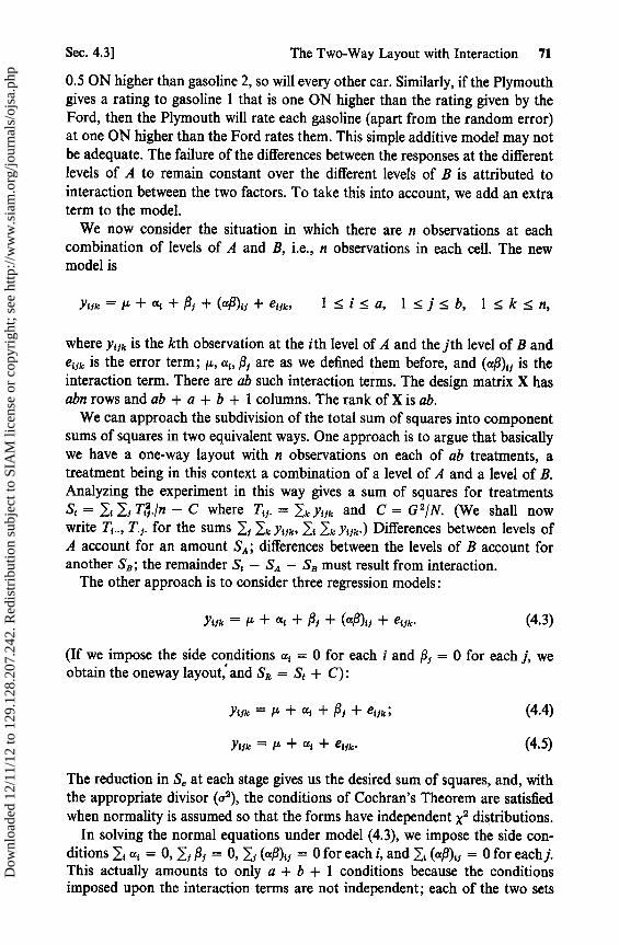
Sec. 4.3] The Two-Way Layout with Interaction 71
0.5 ON higher than gasoline 2, so will every other car. Similarly, if the Plymouthgives a rating to gasoline 1 that is one ON higher than the rating given by theFord, then the Plymouth will rate each gasoline (apart from the random error)at one ON higher than the Ford rates them. This simple additive model may notbe adequate. The failure of the differences between the responses at the differentlevels of A to remain constant over the different levels of B is attributed tointeraction between the two factors. To take this into account, we add an extraterm to the model.
We now consider the situation in which there are n observations at eachcombination of levels of A and B, i.e., n observations in each cell. The newmodel is
Yuk = µ + at + P1 + (aP){f + eilk, 1 < i < a, 1 < j < b, 1 < k < n,
where yifk is the kth observation at the ith level of A and the jth level of B andei1k is the error term; µ, ai , P1 are as we defined them before, and (as)ti is theinteraction term. There are ab such interaction terms. The design matrix X hasabn rows and ab + a + b + 1 columns. The rank of X is ab.
We can approach the subdivision of the total sum of squares into componentsums of squares in two equivalent ways. One approach is to argue that basicallywe have a one-way layout with n observations on each of ab treatments, atreatment being in this context a combination of a level of A and a level of B.Analyzing the experiment in this way gives a sum of squares for treatmentsSt = lt ^f T1./n — C where T11. = Ik Y41k and C = G 2/N. (We shall nowwrite Ti .., T.,. for the sums l f Ik Ytik, ^t Ik Yuk•) Differences between levels ofA account for an amount SA ; differences between the levels of B account foranother SB ; the remainder St — SA — SB must result from interaction.
The other approach is to consider three regression models:
Ytlk = µ + at + jJ + (af1)u + eifk• (4.3)
(If we impose the side conditions a, = 0 for each i and P, = 0 for each j, weobtain the oneway layout, and SR = St + C):
Ytrk = FJ + as + S! + etik; (4.4)
Yuk = i& + a i + eijk. (4.5)
The reduction in Se at each stage gives us the desired sum of squares, and, withthe appropriate divisor (aa), the conditions of Cochran's Theorem are satisfiedwhen normality is assumed so that the forms have independent x2 distributions.
In solving the normal equations under model (4.3), we impose the side con-ditions = 0, If Si = 0, Ii (af1)1J = 0 for each i, and 1t (af1),f = 0 for each j.This actually amounts to only a + b + 1 conditions because the conditionsimposed upon the interaction terms are not independent; each of the two sets
Dow
nloa
ded
12/1
1/12
to 1
29.1
28.2
07.2
42. R
edis
trib
utio
n su
bjec
t to
SIA
M li
cens
e or
cop
yrig
ht; s
ee h
ttp://
ww
w.s
iam
.org
/jour
nals
/ojs
a.ph
p
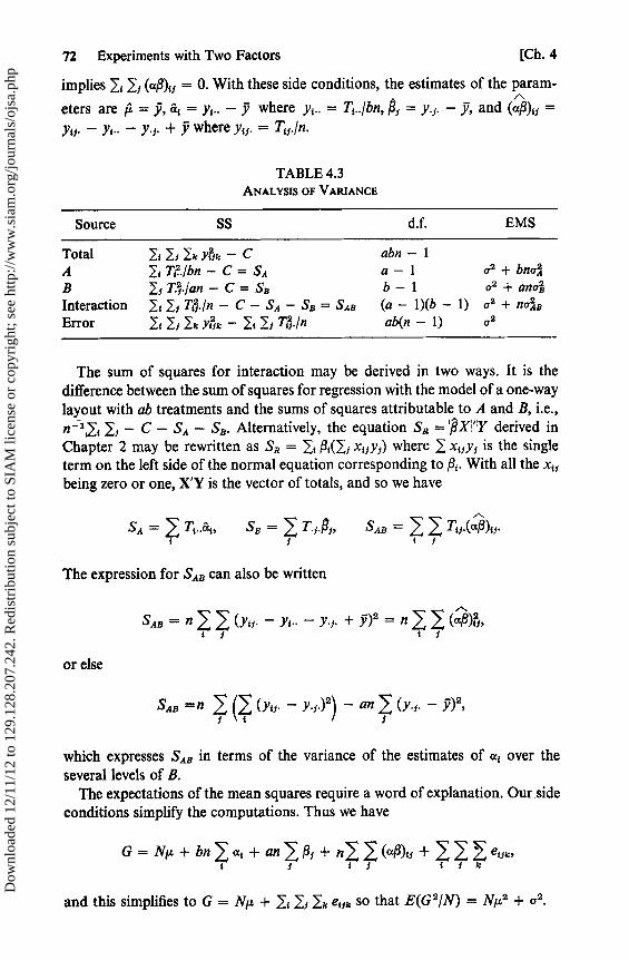
72 Experiments with Two Factors [Ch. 4
implies li I j (aa)i5 = 0. With these side conditions, the estimates of the param-
eters are µ =9,& = yt.. —9 where y,.. = T{ ../bn, ,^, =y.. -7, and ( 1 =yi1. — y t .. — y.,. + y where yif. = T,1./n.
TABLE 4.3ANALYSIS OF VARIANCE
Source SS d.f. EMS
Total li G1 Gk Y41k — C abn — 1A l i T,?./bn — C = SA a — 1 a2 + bna2
B J, T../an — C = SB b — 1 a2 + anaBInteraction 1, J, T!./n — C — SA — SB = SAa (a — 1)(b — 1) aa + naÁ8Error lt I1 Ik Ys1k — lt St T 5./n ab(n — 1) aa
The sum of squares for interaction may be derived in two ways. It is thedifference between the sum of squares for regression with the model of a one-waylayout with ab treatments and the sums of squares attributable to A and B, i.e.,n - ^, ^1 — C — SA — SB . Alternatively, the equation SR = IPX!'IY derived inChapter 2 may be rewritten as SR = li Pt(l1 x{1y,) where 1 xy1 is the singleterm on the left side of the normal equation corresponding to P { . With all the x, i
being zero or one, X'Y is the vector of totals, and so we have
SA = Ti ..«tl SB = L T.5., SAS = Tt1( ^)t1•
The expression for SAB can also be written
SAB =n (yi1.—y1..—y.1.+9)2=n
or else
SAB =n ( (yu. — — an (y.1. — 9) 2,
which expresses SAB in terms of the variante of the estimates of a{ over theseveral levels of B.
The expectations of the mean squares require a word of explanation. Our,sideconditions simplify the computations. Thus we have
G = Np + bn a4 + an 1 P1 + nl 1(afl)t1 + 1 E es>k,1 4 1 f ik
and this simplifies to G = Nµ + Lk euk so that E(G 2/N) = Np 2 + aaDow
nloa
ded
12/1
1/12
to 1
29.1
28.2
07.2
42. R
edis
trib
utio
n su
bjec
t to
SIA
M li
cens
e or
cop
yrig
ht; s
ee h
ttp://
ww
w.s
iam
.org
/jour
nals
/ojs
a.ph
p

Sec. 4.4] The Subdivision of the Sum of Squares for Interaction 73
Similarly, yt .. — y reduces from µ + at + fi. + (af) t . + et .. — µ — a. —^. — (as).. — e..., where e t .. = aN-1 Ii Ik etik and e... = N-1 lt Ii Ik etik to
yt — Y=at+et.. — e...;
thus, E(SA) = bn l t E(y, — 9)2 = bn It aa + (a — 1)02, and we shall, in anobvious notation, write I t at as (a — 1)4
Finally, we can proceed in the same way and obtain
E(SAB) = n: E(yu. — y,.. — y.j. + 9) 2t i
= n (a,6) i + (a — 1)(b — 1)a 2 .t i
We then write It Ii (aa)ti as (a — 1)(b — 1)»ÁB.
4.4 The Subdivision of the Sum of Squares for Interaction
We discussed in the previous chapter the subdivision of the sum of squares fortreatments in the one-way layout. This process can be extended to the factortalexperiment, and the sums of squares for A, B, and AB interaction can all besubdivided into single degrees of freedom. We can take ab — 1 orthogonalcontrasts in the cell totals, of which (a — 1) are contrasts in the A totals and(b — 1) are contrasts in the B totals. The squares of the remaining contrastswith the appropriate divisors each correspond to one degree of freedom, andtheir total is S„B . We mention two uses of this procedure, one of which, Tukey'sone degree of freedom for interaction, will be discussed in the next section.
We have already seen that when A is a quantitative factor, preferably with itslevels equally spaced, SA can be divided into such components as linear, quad-ratic, and cubic. If both A and B are quantitative, this approach can be extendedto fit the model.
a b a b
E(y) = Po + 3toxi + boixá + Ptixixá,t=^ i1 1=15=1
where xl and x2 are coordinates for the levels of A and B respectively. Replacingxi by the ith degree orthogonal polynomial for a levels, u t, and xá by the corre-sponding polynomial vi, we obtain
E(y) = Yo + 1 Ytout + 1 Yoivi + 1 Ytiutvi•
The estimates of the yti are orthogonal contrasts. The contrasts corresponding toyto and yoi are the linear, quadratic, cubic, and so on contrasts for A and B and
Dow
nloa
ded
12/1
1/12
to 1
29.1
28.2
07.2
42. R
edis
trib
utio
n su
bjec
t to
SIA
M li
cens
e or
cop
yrig
ht; s
ee h
ttp://
ww
w.s
iam
.org
/jour
nals
/ojs
a.ph
p
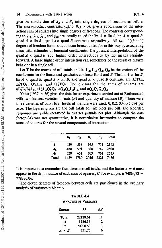
74 Experiments with Two Factors [Ch. 4
give the subdivision of SA and SB into single degrees of freedom as before.The cross-product contrasts, yjj(i > 0,] > 0), give a subdivision of the inter-action sum of squares into single degrees of freedom. The contrasts correspond-ing to yll, Y122 Y21. and yaa are usually called the lin A x lin B, lin A x quad B,quad A x lin B, quad A x quad B contrasts respectively. All (a — 1)(b — 1)degrees of freedom for interaction can be accounted for in this way by associatingthem with estimates of binomial coefficients. The physical interpretation of thequad A x quad B and higher order interactions is by no means straight-forward. A large higher order interaction can sometimes be the result of bizarrebehavior in a single ceil.
Let T be the matrix of cell totals and let LA, LB , Q,, QB be the vectors of thecoefficients for the linear and quadratic contrasts for A and B. The lin A x lin B,lin A x quad B, quad A x lin B, and quad A x quad B contrasts are LATLB ,L ITQ B, QÁTLB, and QÁTQB. The divisors for the sums of squares arenLÁLALéLB, nLALAQBQB, nQ.sQALBLB, and nQQAQQB.
Yates (1937, p. 36) gives the data for an experiment carried out at Rothamstedwith two factors, varieties of oats (A) and quantity of manure (B). There werethree varieties of oats; four levels of manure were used, 0, 0.2, 0.4, 0.6 cwt peracre. The figures given are the celi totals for six plots per cell; the recordedresponses are yields measured in quarter pounds per plot. Although the oatsfactor (A) was not quantitative, it is nevertheless instructive to compute thesums of squares for the several components of interaction.
B1 B2 B3 B4 Total
A l 429 538 665 711 2343Az 480 591 688 749 2508A3 520 651 703 761 2635
Total 1429 1780 2056 2221 7486
It is important to remember that these are cell totals, and the factor n = 6 mustappear in the denominator of each sum of squares; C, for example, is 74861/72 =778336.06.
The eleven degrees of freedom between cells are partitioned in the ordinaryanalysis of variance table into
TABLE 4.4ANALYSIS OF VAIUANCE
Source SS d.f.
Total 22128.61 11A 1786.36 2B 20020.50 3
A x B 321.75 6Dow
nloa
ded
12/1
1/12
to 1
29.1
28.2
07.2
42. R
edis
trib
utio
n su
bjec
t to
SIA
M li
cens
e or
cop
yrig
ht; s
ee h
ttp://
ww
w.s
iam
.org
/jour
nals
/ojs
a.ph
p

Sec. 4.5] Interaction with One Observation per Cell 75
To obtain the interaction contrasts, we first obtain the B contrasts at eachlevel of A by using Lá = (-3, —1, 1, 3), Qá = (1, —1, —1, 1), Cá =(1, —3, 3, —1). Then we multiply by LÁ = (-1,0, 1), QÁ = (-1, 2, —1). Thuslin A x lin B = 775 -973 = —198, and quad A x quad B = 63 — 2(50) +73 = 36. The B contrasts are
lin B quad B cub B A divisor
Al 973 —63 99Aa 904 —50 22A 3 775 —73 —85
lin A ' —198 —10 —184 2quad A 60 36 30 6
B divisors 20 4 20
The individual sums of squares are
lin A x lin Blin A x quad Blin A x cub Bquad A x lin Bquad A x quad Bquad A x cub B
(-198)2/(2 x 20 x 6) = 163.35(-10)2/(2 x 4 x 6) = 2.08
(-184)2/(2 x 20 x 6) = 141.07(60)2/(6 x 20 x 6) = 5.00
(36) 2/(6 x 4 x 6) = 9.00(30)2/(6 x 20 x 6) = 1.25
321.75
The value of the lin A x lin B term is large, and we note that the lin Bcontrast decreases as we change levels of A: 973, 904, 775. (If we had inter-changed varieties 2 and 3, this inconsistency of the lin B contrast would havebeen manifested as a large quad A x lin B interaction; - however, A is not reallya quantitative factor.) It would appear that the increase in the response caused byusing extra manure is greater for A l than for A 3 .
4.5 Interaction with One Observation per Cell
Our earlier discussion of the two-way layout with one observation per cellcame before we introduced the idea of interaction. If there is interaction present,the sum of squares called Se is actually SAB with n = 1. We have, therefore, twoproblems:
(i) Our estimate of the error variance is biased inasmuch as E(M.)a2 + °B;
(ii) We have lost our F test for the hypothesis a = 0.
Dow
nloa
ded
12/1
1/12
to 1
29.1
28.2
07.2
42. R
edis
trib
utio
n su
bjec
t to
SIA
M li
cens
e or
cop
yrig
ht; s
ee h
ttp://
ww
w.s
iam
.org
/jour
nals
/ojs
a.ph
p
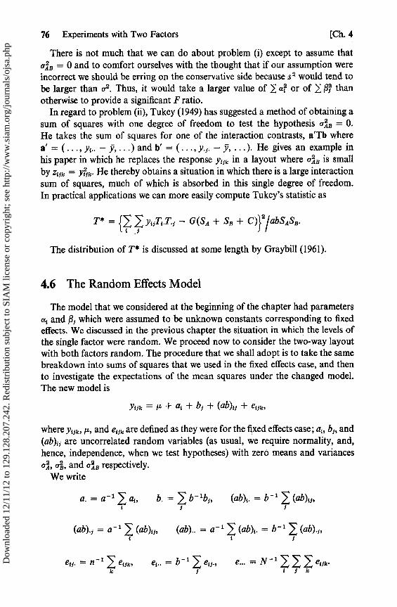
76 Experiments with Two Factors [Ch. 4
There is not much that we can do about problem (i) except to assume thatvAB = 0 and to comfort ourselves with the thought that if our assumption wereincorrect we should be erring on the conservative side because s 2 would tend tobe larger than a2. Thus, it would take a larger value of 1 a? or of fl thanotherwise to provide a significant F ratio.
In regard to problem (ii), Tukey (1949) has suggested a method of obtaining asum of squares with one degree of freedom to test the hypothesis a = 0.
He takes the sum of squares for one of the interaction contrasts, a'Tb wherea' = (... , y{ .. — y, ...) and b' _ (... , y.j . — y, ... ). He gives an example inhis paper in which he replaces the response y ijk in a layout where cÁS is small
by zirk = He thereby obtains a situation in which there is a large interactionsum of squares, much of which is absorbed in this single degree of freedom.In practical applications we can more easily compute Tukey's statistic as
T* _ — G(SA + SE + C)}2 /abSASB .
The distribution of T* is discussed at lome length by Graybill (1961).
4.6 The Random Effects Model
The model that we considered at the beginning of the chapter had parametersa, and $, which were assumed to be unknown constants corresponding to fixedeffects. We discussed in the previous chapter the situation in which the levels ofthe single factor were random. We proceed now to consider the two-way layoutwith both factors random. The procedure that we shall adopt is to take the samebreakdown into sums of squares that we used in the fixed effects case, and thento investigate the expectations of the mean squares under the changed model.The new model is
ytfk = µ + at + bf + (ab)i1 +
where y,ik, µ, and e,ik are defined as they were for the fixed effects case; ai, bj, and(ab), f are uncorrelated random variables (as usual, we require normality, and,hence, independence, when we test hypotheses) with zero means and variances4, oá, and 4B respectively.
We write
a. = a 1 l at , b. = 1 b lbf, (ab),. = b' (ab)ii,i i 1
(ab).; = a -1 (ab)ii, (ab).. = a' (ab)t . = b' > (ab). i,c c f
e{ f. = n -1 1 e,rk, e,.. = b - ' ei f., e... = N1 1 e.k i t 1 k
Dow
nloa
ded
12/1
1/12
to 1
29.1
28.2
07.2
42. R
edis
trib
utio
n su
bjec
t to
SIA
M li
cens
e or
cop
yrig
ht; s
ee h
ttp://
ww
w.s
iam
.org
/jour
nals
/ojs
a.ph
p
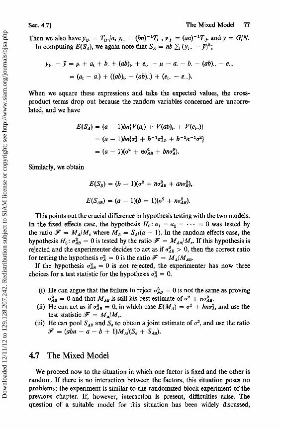
Sec. 4.7] The Mixed Model 77
Then we also have yti. = T 1./n, yi.. _ (bn) - 'Ti .., y.f. = (an) - 'T. 1 . and y = GEN.In computing E(SA), we again note that SA = nb (y f .. — y)2 ;
y{..—y= µ + a,+b.+(ab),.+e,..—µ—a.—b.—(ab)..—e...
= (ai — a.) + ((ab). — (ab)..) + (ei.. — e...).
When we square these expressions and take the expected values, the cross-product terms drop out because the random variables concerned are uncorre-lated, and we have
E(SA) = (a — 1)bn{V(a 1) + V(ab) 1. + V(et ..)}
= (a — 1)bn{aÁ + b -laAB + b - 1n -1a2}
= (a — 1)(62 + natB + bnaÁ).
Similarly, we obtain
E(SB) = (b — 1)(a2 + naA2B + anaá),
E(SAB) = (a — 1)(b — 1)(a 2 + noáB)•
This points out the crucial difference in hypothesis testing with the two models.In the fixed effects case, the hypothesis Ho : al = = • • • = 0 was tested bythe ratio F = M4/Me where MA = SA/(a — 1). In the random effects case, thehypothesis H0 : oAB = 0 is tested by the ratio .F = MABI M,. If this hypothesis isrejected and the experimenter decides to act as if aAB > 0, then the correct ratiofor testing the hypothesis a = 0 is the ratio .W = MA/MAB .
If the hypothesis oÁB = 0 is not rejected, the experimenter has now threechoices for a test statistic for the hypothesis QÁ = 0.
(i) He can argue that the failure to reject vÁB = 0 is not the same as provingaA, = 0 and that MAB is still his best estimate of o2 + naAB.
(ii) He can act as if vÁB = 0, in which case E(MA) = 02 + bnaA2, and use thetest statistic JF = MA/M€ .
(iii) He can pool SAB and Se to obtain a joint estimate of a2, and use the ratio= (abn — a — b + 1)MA/(Se + SAB)•
4.7 The Mixed Model
We proceed now to the situation in which one factor is fixed and the other israndom. If there is no interaction between the factors, this situation poses noproblems; the experiment is similar to the randomized block experiment of theprevious chapter. If, however, interaction is present, difficulties arise. Thequestion of a suitable model for this situation has been widely discussed,
Dow
nloa
ded
12/1
1/12
to 1
29.1
28.2
07.2
42. R
edis
trib
utio
n su
bjec
t to
SIA
M li
cens
e or
cop
yrig
ht; s
ee h
ttp://
ww
w.s
iam
.org
/jour
nals
/ojs
a.ph
p

78 Experiments with Two Factors [Ch. 4
particularly by Wilk and Kempthorne (1955) and (1956), by Scheffé (1956a and b),and by Cornfield and Tukey (1956). The approaches of Cornfield and Tukey andof Wilk and Kempthorne involve deriving the expected values on the assumptionthat the levels of the fixed factor A are a random sample of size a from a finitepopulation of size p, and then putting p equal to a. We shall follow Scheffé'sderivation. Again, we take the breakdown into sums of squares derived for thefixed effects case, and concern ourselves with the expected values of those sumsof squares under the new conditions.
The new model is
Yifk= µ+ ai +b! +Cij +eifk;
Yuk, µ, b1, and e,i,, are defined in the same way as in the random effects model,and the bi and the eifk are all uncorrelated; the effects at are unknown constantssubject to the side condition 1 a, = 0; c,i is the interaction term.
The interactions c15 are random variables: they involve a random factor B.They are not correlated with any of the bi or the etfk . However, bearing in mindthat for the fixed effects a, we have 1 ai = 0, we impose a similar condition
c,5 = 0 for each j upon the interaction terms. Consequently, the c{j are, forany given j, correlated with each other. It is convenient to write V(c 1) as(a — 1 )aÁS/a.
Lemma. Let xl , x2 ,. . . , x, be a set of random variables having the same variancea2 and the same covariances pat, and being subject to the condition x, = const;then p = —(n — 1) -1 .PR00F. We have V(I x,) = na2 + n(n — l)pQa. But 1 x, = const impliesthat V(I xi) = 0. Hence, n(1 + (n — l)p)a2 = 0, and so p = —(n — 1) -1. •
Applying this lemma to the c,i, with n = a and a2 = (a — l)oÁS/a, we havefor i 96 i', j 0 j'
cov (cij, c1 . 5) = —a -1QAB, cov (cjj , ct5 ) = cov (ctf, c,.1.) = 0,
V(ci .) = b - 'V(cu) = b-la -1(a — 1)QA B .
We proceed now to derive the expectations of the sums of squares.
E(Se) = ab(n — 1)a2 , (4.6)
as before.
SA = bn I (Yt.. — y)2 .s
(Y..—y)=a,—a.+b.—b.+ c 1. — c.. + et .. — e...
= at+ci.+ei..—e...,
Dow
nloa
ded
12/1
1/12
to 1
29.1
28.2
07.2
42. R
edis
trib
utio
n su
bjec
t to
SIA
M li
cens
e or
cop
yrig
ht; s
ee h
ttp://
ww
w.s
iam
.org
/jour
nals
/ojs
a.ph
p

Sec. 4.7] The Mixed Model 79
since a. = 0 and c.. = 0. Thus, E(SA) = bn 1 a? + n(a — 1)aÁ B + (a — 1)a2 ,and writing 1 a? = (a — 1)oÁ,
E(MA) = a2 + naL + bnaÁ. (4.7)
Ss = an (Y.. — y)a .
(y.,. — Y)=a. — a.+b5 — b.+ c.1 — c.. + e.5 . — e...
=bf —b.+e. 1.—e...,
since c.1 = c.. = 0. Then
E(SB) = an(b — 1){V(b1) + V(e.J.)} = (b — 1)(a2 + anuB),
E(MB) = aa + an4B. (4.8)
Sas = n (Y,1. — y{ .. — Y.J. + 7)2 ,^ r
(Yii. — y,.. — y. i. + y) = c,f — c{. + (et1. — e,.. — e. j. + e...) .
The error term is the same term that appears in the earlier models; its contribu-tion to E(SAB) is (a — 1)(b — l)a2 . E{I5 (cij — c,.) 2} = (b — 1)V(c15) for each i.Hence, E(SAB) = (a — 1)(b — 1)(a2 + nOÁB), and
E(MAB) = a2 + na. (4.9)
From this, we see that if a4B 0 0, the hypothesis QÁ = 0 is tested by the ratio= MA/MAB , while the hypothesis o8 = 0 is tested by .5F = MB/Me .
If there is only one observation per cel!, S e does not exist, and we have onlythe three sums of squares SA, SB, and SAB . In the random effects case, thispresents no problem in testing oÁ = 0 or oB = 0 because MAB is the appropriatedenominator for the test statistic anyway. However, in the fixed effects case (andin the mixed case considered in this section when we test QB = 0), there is notest for the main effects unless it can be assumed a priori that a3 = 0.
Some people find it surprising that although A is a fixed effect, its expectedmean square contains the interaction term (4B, which would appear at firstglance to go with A random rather than with A fixed. The approaches of Wilkand Kempthorne and of Cornfield and Tukey throw more light on this. Theyobtain E(MA) as
E(MA) = a2 + (1 — b/R)(Á6 + bna4,
and
where
Dow
nloa
ded
12/1
1/12
to 1
29.1
28.2
07.2
42. R
edis
trib
utio
n su
bjec
t to
SIA
M li
cens
e or
cop
yrig
ht; s
ee h
ttp://
ww
w.s
iam
.org
/jour
nals
/ojs
a.ph
p

80 Experiments with Two Factors [Ch. 4
where q denotes the number of levels of B in the population of levels from whichthe experimenter chose the b levels actually used.
Then, if B is fixed, b = q and (1 — b/q) = 0; but, if B is random, q = co and(1 — b/q) = 1. We may also picture ourselves, when looking at the main effectsof A, as averaging the interactions cij over all the levels of B that were used. If Bis fixed, then we have averaged over all possible levels of B, and the interactionterms "cancel out"; on the other hand, if Bis a random factor, we are averagingover only a fraction of the levels of B, and it would not be reasonable to assumethat the interactions average out in any given experiment.
4.8 The Two-Stage Nested or Hierarchic Design
We illustrate this design by an example. Consider b batches of gasolineproduced by some process. From each batch, s samples are taken, and then nobservations are made on the octane number of each sample. If y,fk denotes thekth observation on the jth sample from the ith batch, we have
YiJk = µ + b, + si(> + e,cin,
where bi is the effect of the ith batch, s„, ) is the effect of the jth sample in the ithbatch, and ek(tn is the observational error.
If we assume to begin with that µ, b, and s,( , ) are all fixed, we have bs samplesand 1 + b + bs parameters. We impose side conditions 1i b, = 0 and I1 sf( ,) = 0for each i. Then, if yij. and y,.. denote the sample and batch means,
µ = Y, bi = Yi.. — Y, s'j(i) = Yj. — y{ ...
The sum of squares attributable to batch differences is obtained by treating thesetup as just a one-way layout with b batches and sn observations per batch,which gives
SB = T?./ns — G 2/N,
where N = bsn. Regarding the set-up as a one-way layout with bs samples andn observations pet sample gives a sum of squares
SR =T1./n —Ga/N.
Then, subtracting, we have the sum of squares for samples within batches, as
Ss in a = SS(B) _ T>•ln — Tt?•lns ;s i 1
Dow
nloa
ded
12/1
1/12
to 1
29.1
28.2
07.2
42. R
edis
trib
utio
n su
bjec
t to
SIA
M li
cens
e or
cop
yrig
ht; s
ee h
ttp://
ww
w.s
iam
.org
/jour
nals
/ojs
a.ph
p

Sec. 4.9] The Diallel Cross Experiment 81
and also
Se = Yttk — Tiran.1 r k t j
Alternatively, we may argue that SB = lt Fi{T.. and Ss(B) _ ^{ ^i sj(,)Tf.. Theetension to more than two stages is obvious.
If either of the two factors is random, we take the same breakdown into sumsof squares. The most common situation is that in which S is a random effect, thesf(, ) being (normally) distributed with mean zero and variance oi. We write vófor V(e,Jk). We shall assume that the batches are distributed with mean zero andvariance az. An example from genetics is the case of s sires being chosen andeach of them being mated to d dams (there being ds dams altogether); then nsiblings are chosen from each of the ds litters. The expectations of the meansquares are given in Table 4.5.
TABLE 4.5ANALYSIS OF VARIANCE
Source SS d.f. EMS
Total LL IkYlk-C N-1Between sires 2, T2./dn — C s — 1 aó + na + dna2
Dams in sires li 21 Taf./n — 2, T?./dn s(d — 1) aó + noiBetween siblings 1, I f lkYuk — l+ 1i Tƒ./n sd(n — 1) ao
Under normality, the testing of the hypotheses oi = 0 and a = 0 is carried outby the F test in the usual way. The principal interest in the experiment usuallycenters, however, on the problems of estimating the components of variancevó, ai, and 1.
4.9 The Diallel Cross Experiment
This kind of experiment is commonly performed by geneticists who areinterested in selecting lines and strains of plants or animals for further breeding.The structure of the model used is similar to that of the two-way layout withinteraction. Observations are made on the offspring of the crosses of pairs ofinbred lines. The main effect of a given line is called its general combiningability, a term originally defined by Sprague and Tatum (1942). Correspondingto the interaction terms in the two-way layout are the specific combining abilities.The reader is referred for a more detailed discussion to the papers by Griffing(1956) and Kempthorne (1956b).
We consider here a situation in which p inbred lines are chosen and somecrosses are made. Griffing discusces four different experiments. In methods 1 and2 the p parental lines are also included; in methods 3 and 4 they are omitted.In methods 1 and 3 the reciprocal crosses are included, i.e., both the cross in
Dow
nloa
ded
12/1
1/12
to 1
29.1
28.2
07.2
42. R
edis
trib
utio
n su
bjec
t to
SIA
M li
cens
e or
cop
yrig
ht; s
ee h
ttp://
ww
w.s
iam
.org
/jour
nals
/ojs
a.ph
p
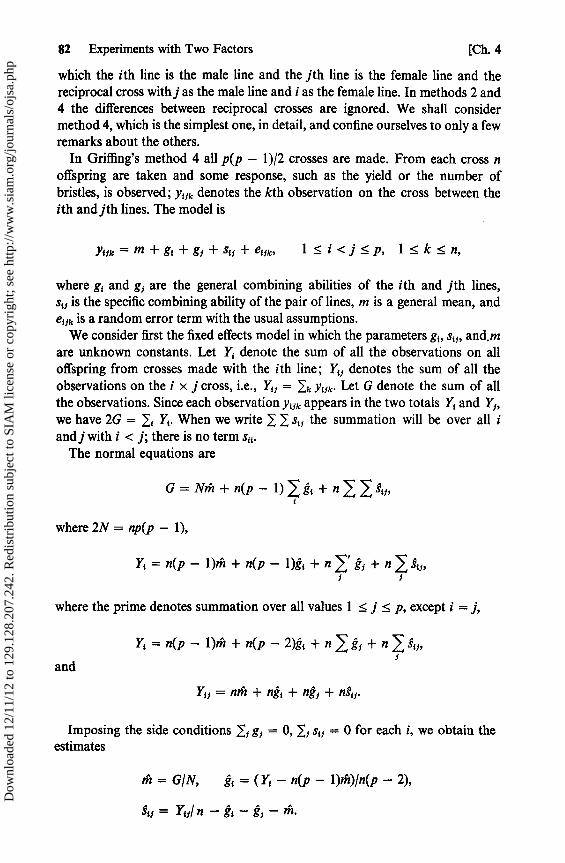
82 Experiments with Two Factors [Ch. 4
which the ith line is the male line and the jth line is the female line and thereciprocal cross withj as the male line and i as the female line. In methods 2 and4 the differences between reciprocal crosses are ignored. We shall considermethod 4, which is the simplest one, in detail, and confine ourselves to only a fewremarks about the others.
In Griffing's method 4 all p(p — 1)/2 crosses are made. From each cross noffspring are taken and some response, such as the yield or the number ofbristles, is observed; Y,ik denotes the kth observation on the cross between theith and jth lines. The model is
y,ik =m+gi +gi +s{i +e,ik, 1 <i<j<p, 1 <k<n,
where g, and g; are the general combining abilities of the ith and jth lines,s„ is the specific combining ability of the pair of lines, m is a general mean, ande{ik is a random error term with the usual assumptions.
We consider first the fixed effects model in which the parameters g { , stƒ, and.mare unknown constants. Let Y; denote the sum of all the observations on alloffspring from crosses made with the ith line; YY1 denotes the sum of all theobservations on the i x j cross, i.e., Yt1 = y. Let G denote the sum of allthe observations. Since each observation y,fk appears in the two totals Yt and Yi,we have 2G = Y. When we write 1 1 s ii the summation will be over all iand j with i < j; there is no term si{ .
The oormal equations are
G=Nm+ n(p — 1) +
where 2N = np(p — 1),
Yi =n(p — 1)m+ n(p — 1)gt +n gf+n>su,
where the prime denotes summation over all values 1 < j < p, except i = j,
Yi =n(p — 1)m+ n(p —2)g { +n1gf +n ti ,
and
=nm+ngt+ng1+nsii.
Imposing the side conditions _7, g; = 0, If stj = 0 for each i, we obtain theestimates
m = GIN, 81 = (YY — n(p — 1)m)/n(p — 2),
gu = YY/ n — g^ — gi — m.
Dow
nloa
ded
12/1
1/12
to 1
29.1
28.2
07.2
42. R
edis
trib
utio
n su
bjec
t to
SIA
M li
cens
e or
cop
yrig
ht; s
ee h
ttp://
ww
w.s
iam
.org
/jour
nals
/ojs
a.ph
p
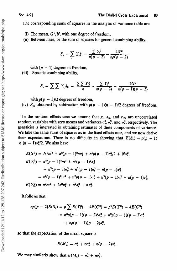
Sec. 4.9] The Diallel Cross Experiment 83
The corresponding sums of squares in the analysis of variance table are
(i) The mean, G'/N, with one degree of freedom,(ii) Betv ,een lines, or the sum of squares for general combining ability,
Ya 4G2Sg yi81=
n(p -2) np(p - 2)
with (p — 1) degrees of freedom,(iii) Specific combining ability,
ya2 Y12 2G2Sa = Yii^{j = n n(p — 2) + n(p — 1 )(p — 2)
with p(p — 3)/2 degrees of freedom,(iv) Se, obtained by subtraction with p(p — 1)(n — 1)/2 degrees of freedom.
In the random effects case we assume that g,, s, l, and e,ik are uncorrelatedrandom variables with zero means and variances a, o$, and aé, respectively. Thegeneticist is interested in obtaining estimates of these components of variance.We take the same sums of squares as in the fixed effects case, and we now derivetheir expectations. There is no difficulty in showing that E(Se) = p(p — 1)x (n — 1)u/2. We also have
E(G 2) = N 2m2 + n2(p — l)2pa + n2p(p — 1)o$/2 + No,
E(Y?) = n2(p — 1 )2m2 + n2(p — 1 )2a2
+ n2(p — 1)a + n 2(p — 1)a$ + n(p — 1)aé
= n2(p — 1 )2m2 + n 2p(p — 1 )aá + n2(p — 1 )aá + n(p — 1 )°é,E(Y f) = n2m2 + 2n2a + n2a + na.
It follows that
np(p — 2)E(S9) = p 1 E( Y?) — 4E(G 2) = p 2E(Ya) — 4E(G 2)
n2p(p — 1 )(p — 2)2aá + n2p(p — 1 )(p — 2)a,
+ np(p — 1 )(p — 2)4
so that the expectation of the mean square is
E(M9) = ae + na; + n(p — 2)4
We may similarly show that E(M) = oé + na;.
Dow
nloa
ded
12/1
1/12
to 1
29.1
28.2
07.2
42. R
edis
trib
utio
n su
bjec
t to
SIA
M li
cens
e or
cop
yrig
ht; s
ee h
ttp://
ww
w.s
iam
.org
/jour
nals
/ojs
a.ph
p
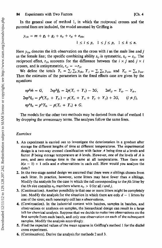
84 Experiments with Two Factors [Ch. 4
In the general case of method 1, in which the reciprocal crosses and theparental lines are included, the model assumed by Griffing is
Ytrk = m + gt + Sr + st) + rti + etrk,
1_<i<p, 1<j<p, 1<k<n.
Here y, jk denotes the kth observation on the cross with i as the male line and jas the female line; the specific combining ability s, ƒ is symmetric, s,i = s5{. Thereciprocal effect, rt,, accounts for the difference between the i x j and j x icrosses, and is antisymmetric, rtj = — rfi .
We define the totals Yt . = I i I k Ytrk, Y> = ^t I k Ytjk, and Y 5 . = I k Yt,k-Then the estimates of the parameters in the fixed effects case are given by theequations
np'th = G, 2np2g{ = 2p(Yi . + Y.,) — 2G, 2nrti = Yt f. —
2np2sti = p2(Y5. + Y,t•) — p(Y1. + Y. t + Y1. + Y.t) + 2G, (i 0 j),
npagtt = p2 Y0 . — p(YY . + Y. t) + G.
The models for the other two methods may be derived from that of method 1by dropping the unnecessary terms. The analyses follow the same lines.
Exercises
1. An experiment is carried out to investigate the deterioration in a product afterstorage for different lengths of time at different temperatures. The experimentaldesign is a two-way crossed classification with factor A being time at a levels andfactor B being storage temperature at b levels. However, one of the levels of A iszero, and zero storage time is the same at all temperatures. Thus there areb(a — 1) + 1 cells and n observations in each cell. How would you analyze thedata ?
2. In the two-stage nested design we assumed that there were n siblings chosen fromeach litter. In practice, however, some litters may have fewer than n siblings.Modify the analysis for the case in which the cell corresponding to the jth litter bythe ith sire contains ntj members where nij > 0 for all i and j.
3. (Continuation). Another possibility is that one or more litters might be completelylost. Modify the analysis for the situation in which there are only d — 1 litters byone of the sires; each nonempty cell has n observations.
4. (Continuation). In the industrial context with batches, samples in batches, andobservations or analyses on samples, the hierarchical design can result in a largebili for chemical analysis. Suppose that we decide to make two observations on thefirst sample from each batch, and only one observation on each of the subsequentsamples. Modify the analysis accordingly.
5. Find the expected values of the mean squares in Griffing's method 1 for the diallelcross experiment.
6. (Continuation). Derive the analysis for methods 2 and 3.
Dow
nloa
ded
12/1
1/12
to 1
29.1
28.2
07.2
42. R
edis
trib
utio
n su
bjec
t to
SIA
M li
cens
e or
cop
yrig
ht; s
ee h
ttp://
ww
w.s
iam
.org
/jour
nals
/ojs
a.ph
p
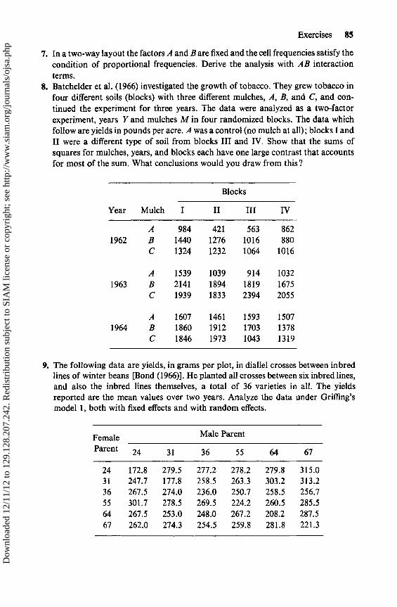
Exercises 85
7. Ina two-way layout the factors A and B are fixed and the cell frequencies satisfy thecondition of proportional frequencies. Derive the analysis with AB interactionterms.
8. Batchelder et al. (1966) investigated the growth of tobacco. They grew tobacco infour different soils (blocks) with three different mulches, A, B, and C, and con-tinued the experiment for three years. The data were analyzed as a two-factorexperiment, years Y and mulches M in four randomized blocks. The data whichfollow are yields in pounds per acre. A was a control (no mulch at all); blocks 1 andII were a different type of soil from blocks III and IV. Show that the soms ofsquares for mulches, years, and blocks each have one large contrast that accountsfor most of the sum. What conclusions would you draw from this?
Year Mulch I
Blocks
II III IV
A 984 421 563 8621962 B 1440 1276 1016 880
C 1324 1232 1064 1016
A 1539 1039 914 10321963 B 2141 1894 1819 1675
C 1939 1833 2394 2055
A 1607 1461 1593 15071964 B 1860 1912 1703 1378
C 1846 1973 1043 1319
9. The following data are yields, in grams per plot, in diallel crosses between inbredlines of winter beans [Bond (1966)]. He planted all crosses between six inbred lines,and also the inbred lines themselves, a total of 36 varieties in all. The yieldsreported are the mean values over two years. Analyze the data under Griffing'smodel 1, both with fixed effects and with random effects.
Female Male Parent
Parent 24 31 36 55 64 67
24 172.8 279.5 277.2 278.2 279.8 315.031 247.7 177.8 258.5 263.3 303.2 313.236 267.5 274.0 236.0 250.7 258.5 256.755 301.7 278.5 269.5 224.2 260.5 285.564 267.5 253.0 248.0 267.2 208.2 287.567 262.0 274.3 254.5 259.8 281.8 221.3
Dow
nloa
ded
12/1
1/12
to 1
29.1
28.2
07.2
42. R
edis
trib
utio
n su
bjec
t to
SIA
M li
cens
e or
cop
yrig
ht; s
ee h
ttp://
ww
w.s
iam
.org
/jour
nals
/ojs
a.ph
p
CHAPTER 5
Experimentswith
Several Factors
The results obtained in the previous chapter can be extended to larger experi-ments involving more than two factors. The simplest situation is the completefactorial experiment in which all the factors are fixed and crossed. This is aroutine extension of the two-way crossed classification. The term crossedclassification is used to denote that each factor is crossed with the others:factor A cuts across factor B in the sense that each level of factor A appears witheach level of factor B.
We shall see that in the crossed classification with some of the factors randomcomplications can arise about the Ftests. In some cases, no one mean square willprovide a suitable denominator for the F statistic to test a hypothesis, and adenominator has to be put together from several mean squares. We shall alsoconsider designs that contain both crossed and nested factors. A set of rules will begiven for deriving the degrees of freedom, sums of squares, and the expectationsof the mean squares. The chapter ends with a short discussion, including someexamples, of split-plot and split-split-plot designs. Before proceeding further, itis appropriate to make a few remarks about error terms, pooling, and replicates.
5.1 Error Terms and Pooling
We have seen in the previous chapter that in a two-way layout with a singleobservation per cell we do not have an estimate of the error variance unless weare prepared to assume, a priori, that there is no interaction between the twofactors. This situation persists when there are more than two factors, and it is ageneral operating procedure that if there is only one observation per cell, the
EA
Dow
nloa
ded
12/1
1/12
to 1
29.1
28.2
07.2
42. R
edis
trib
utio
n su
bjec
t to
SIA
M li
cens
e or
cop
yrig
ht; s
ee h
ttp://
ww
w.s
iam
.org
/jour
nals
/ojs
a.ph
p

Sec. 5.2] Replicates 87
highest order interaction (the interaction between all the factors) is taken to bezero, a priori. If the experimenter does not want to assume this in any caseexcept that in which all the effects are random, he will have to find some way ofduplicating his observations to obtain an unbiased estimate of error. If severalof the factors are at more than two levels, this procedure of ignoring the highestorder interaction will provide an error term with a reasonable number ofdegrees of freedom.
If an experiment involves four factors, each at four levels, the ABCD inter-action will have 3 4 = 81 d.f. Assuming the effects to be fixed, the critical valueof F for testing the hypothesis that the main effects for A are zero, using a = 0.05,is F*(3, 81), which is approximately 2.7. If the factors are at only three levelseach, we should have 16 d.f. for ABCD and F*(3, 16) = 3.24, which meansthat we should need a 20 per cent larger F value in order to detect differencesbetween the levels of A, a considerable decrease in power. If all the factors are attwo levels each, there will only be a single degree of freedom for each of the meansquares. In the Jatter circumstances, the experimenter is going to be ratherdesperate for degrees of freedom in the denominators of his F statistirs, and it iscustomary in such experiments to assume, in the absence of information tothe contrary, that all interactions involving more than two factors are negligible,a priori, and to pool their sums of squares to obtain an error term. We shalltacitly make that assumption in the later chapters when we discuss experimentswith factors at two or three levels.
The pooling of interaction sums of squares to provide an error term is asubjective matter. On the one hand, purists can deplore the use of a possiblybiased denominator and a possibly invalid F statistic. On the other hand, thepractical man can hardly be condemned for making use of reasonable assump-tions to obtain enough degrees of freedom in the denominator for his F test tohave enough power to be useful. What is important is that the experimentershould use his common sense. There used to be a popular procedure, which hashopefully passed into disuse, by which the experimenter would start his F testsat the foot of the table, testing the mean square in the next to last line against themean square for the error. If the ratio was larger than the critical value of F,he recorded the fact in the right-hand column and moved on to the next line.If the ratio was not significant, he pooled the sum of squares with the errorterm and went on to the next line. So he continued up the table automaticallypooling every sum of squares that was not significant, oblivious to the fact thatjust because the F ratio is not quite big enough for significance it does notnecessarily follow that the hypothesis is true and that if you pool a sum ofsquares that is almost large enough to be significant you will infláte your errorestimate and bias it upward.
5.2 Replicates
The word replicate (or replication) commonly occurs in the jargon of experi-mental design, but its meaning is not always the same. When in later chapters we
Dow
nloa
ded
12/1
1/12
to 1
29.1
28.2
07.2
42. R
edis
trib
utio
n su
bjec
t to
SIA
M li
cens
e or
cop
yrig
ht; s
ee h
ttp://
ww
w.s
iam
.org
/jour
nals
/ojs
a.ph
p
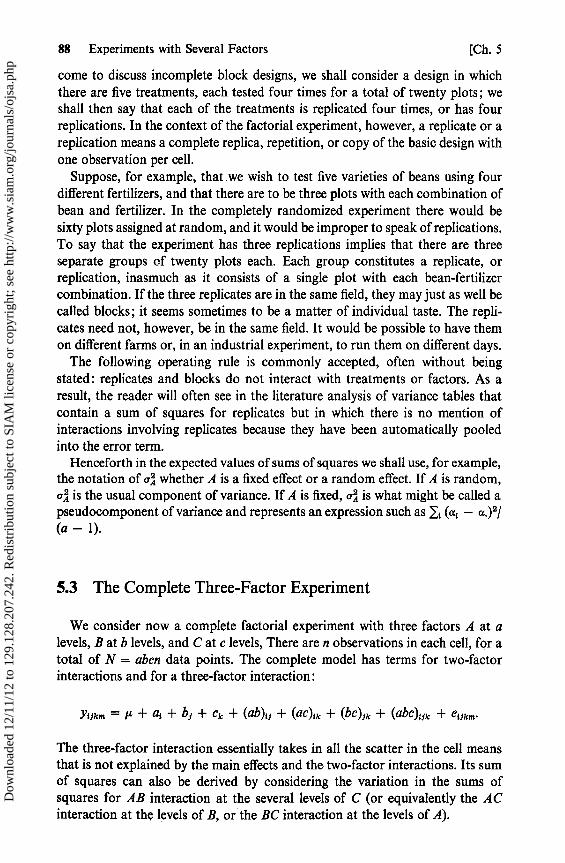
88 Experiments with Several Factors [Ch. 5
come to discuss incomplete block designs, we shall consider a design in whichthere are five treatments, each tested four times for a total of twenty plots; weshall then say that each of the treatments is replicated four times, or has fourreplications. In the context of the factorial experiment, however, a replicate or areplication means a complete replica, repetition, or copy of the basic design withone observation per cell.
Suppose, for example, that .we wish to test five varieties of beans using fourdifferent fertilizers, and that there are to be three plots with each combination ofbean and fertilizer. In the completely randomized experiment there would besixty plots assigned at random, and it would be improper to speak of replications.To say that the experiment has three replications implies that there are threeseparate groups of twenty plots each. Each group constitutes a replicate, orreplication, inasmuch as it consists of a single plot with each bean-fertilizercombination. If the three replicates are in the same field, they may just as well becalled blocks; it seems sometimes to be a matter of individual taste. The repli-cates need not, however, be in the same field. It would be possible to have themon different farms or, in an industrial experiment, to run them on different days.
The following operating rule is commonly accepted, often without beingstated: replicates and blocks do not interact with treatments or factors. As aresult, the reader will often see in the literature analysis of variance tables thatcontain a sum of squares for replicates but in which there is no mention ofinteractions involving replicates because they have been automatically pooledinto the error term.
Henceforth in the expected values of sums of squares we shall use, for example,the notation of aÁ whether A is a fixed effect or a random effect. If A is random,oÁ is the usual component of variance. If A is fixed, a is what might be called apseudocomponent of variance and represents an expression such as _7{ (a{ — a.)2/(a — 1).
5.3 The Complete Three-Factor Experiment
We consider now a complete factorial experiment with three factors A at alevels, B at b levels, and C at c levels, There are n observations in each cell, for atotal of N = abcn data points. The complete model has terms for two-factorinteractions and for a three-factor interaction:
YiJk. = !L + ai + bi + ck + (ab) 1 + (ac),k + (bc)ik + (abc)tik + e{jkm•
The three-factor interaction essentially takes in all the scatter in the cell meansthat is not explained by the main effects and the two-factor interactions. Its sumof squares can also be derived by considering the variation in the sums ofsquares for AB interaction at the several levels of C (or equivalently the ACinteraction at the levels of B, or the BC interaction at the levels of A).
Dow
nloa
ded
12/1
1/12
to 1
29.1
28.2
07.2
42. R
edis
trib
utio
n su
bjec
t to
SIA
M li
cens
e or
cop
yrig
ht; s
ee h
ttp://
ww
w.s
iam
.org
/jour
nals
/ojs
a.ph
p
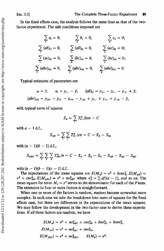
Sec. 5.3] The Complete Three-Factor Experiment 89
In the fixed effects case, the analysis follows the same lines as that of the two-factor experiment. The side conditions imposed are
lat =0,t
(ab)t, = 0,
(ac)tk = 0,
(abc)uk = 0 ,
b1 = 0,
(ab)t1 = 0,
(bc)1k = 0,k
(abc)t1k = 0 ,
Ck 0;k
(ac)tk = 0;k
(bc)1k = 0 ;
(abc)11k = 0 .k
Typical estimates of parameters are
F^ =7, at = Yt... — y, (ab)11 = Y{1.. — yt ... — y.1.. + y,
(abC)t5k = Yt5k• — Yt1.. — yt .k. — y.1k. + yt ... + y. 1.. + y..k . — y r
with typical sums of squares
SA = T?../bcn — C{
witha— 1 d.f.,
SAB=Tu../cn — C — SA — SB,t 1
with (a — 1)(b — 1) d.f.,
SABC=111 Tfk./n — C — SA — SB — SC— SAB — SAC — SBCt 1 k
with (a — 1)(b — 1)(c — 1) d.f..The expectations of the mean squares are E(MA) = a' + bcnaA2, E(MAB) _
oa + cnaA2B, E(MABC) = a 2 + naABC where aÁ = >_ aa/(a — 1), and so on. Themean square for error Me = Sa serves as the denominator for each of the F tests.The extension to four or more factors is straightforward.
When one or more of the factors is random, matters become somewhat morecomplex. In each case we take the breakdown into sums of squares for the fixedeffects case, but there are differences in the expectations of the mean squares.We may follow the development in the two-factor case to derive these expecta-tions. If all three factors are random, we have
E(MA) = aa + nUABC + CnaAB + bnaAC + bcnaA2,
E(MAB) = a2 + naA2BC + cnaA2B,
E(MABC) = a2 + naABC, E(M8) = aa.
Dow
nloa
ded
12/1
1/12
to 1
29.1
28.2
07.2
42. R
edis
trib
utio
n su
bjec
t to
SIA
M li
cens
e or
cop
yrig
ht; s
ee h
ttp://
ww
w.s
iam
.org
/jour
nals
/ojs
a.ph
p

90 Experiments with Several Factors [Ch. 5
For the mixed model, we recall that in the two-factor case with A fixed and Brandom, the term oMB did not appear in E(MB) because for each level of B theinteractions were averaged over the entire set of levels of the fixed factor A.On the other hand, O B did appear in E(MA) because for each level of A theinteractions were averaged over only those b levels of B that were (randomly)chosen from the infinite population.
With this in mind, we can formulate a set of rules for writing down theexpectations of the mean squares in the complete factorial experiment which areapplicable to any number of factors, fixed or random.
1. Each expected mean square contains a term aa.
2. Each component of variance has some letters as subscripts. The coefficientof a component in any expectation is the product of all the letters that are notamong its subscripts. Thus, in the three-factor case we have the four lettersa, b, c, and n. The coefficient of QÁB whenever it appears is the product cn;similarly, we have fla Bc and bcn4 The coefficient is the number of observationscontained in the corresponding total, such as Ti,...
3. If all the factors in an experiment are random, the expectation of a meansquare consists of o2 together with all the terms for effects and interactionscontaining all the letters in the name of the mean square in question. Thus,E(MAB) contains terms for all components with both A and B among thesubscripts, e.g., a2 + nUÁBC + cnOÁ9.
4. If some of the factors are fixed, we strike out in the expectation of any meansquare all those components which have amóng their subscripts any letters,other than those in the name of the mean square, which correspond to fixedfactors. For example, in the three-factor case we have, when all three factors arerandom,
E(MA) = a2 + noÁec + CnvOB + bnalc + bcnoÁ .
Whether A is fixed or random has no bearing on E(MA). However, if C werefixed, we should strike out all terms with C as a subscript and obtain
E(MA) = a2 + cnaÁ$ + bcnaÁ.
If B were also fixed, we should have E(MA) = a2 + bcnaÁ.We give in Table 5.1 the expected mean squares for a three-factor experiment
in three cases:
(i) A, B, and C are all random;(ii) A and B are random, C is fixed;(iii) A is random, B and C are fixed.
In the right-hand column we list the mean square that is the denominator in theF test for the hypothesis that the corresponding effects or interactions or com-ponents of variance are zero. An asterisk denotes that we have to construct a
Dow
nloa
ded
12/1
1/12
to 1
29.1
28.2
07.2
42. R
edis
trib
utio
n su
bjec
t to
SIA
M li
cens
e or
cop
yrig
ht; s
ee h
ttp://
ww
w.s
iam
.org
/jour
nals
/ojs
a.ph
p
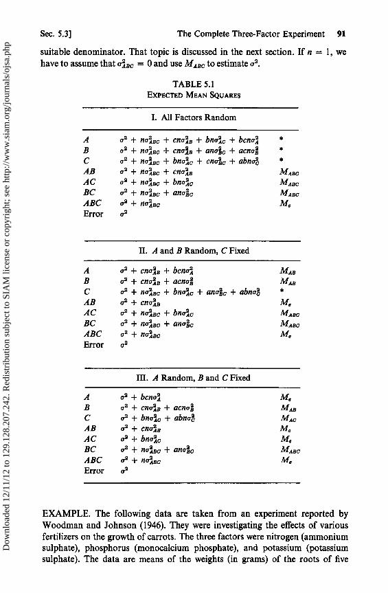
Sec. 5.3] The Complete Three-Factor Experiment 91
suitable denominator. That topic is discussed in the next section. If n = 1, wehave to assume that aAeC = 0 and use MARC to estimate a2 .
TABLE 5.1EXPECTED MEAN SQUARES
I. All Factors Random
A a2 + naABC + cnaAB + bnaAc + bcnaÁ *B a2 + naÁac + cnaÁB + analc + acnoC a2 + naÁBC + bn4 c + cn4Bc + abna2AB a2 + na4ac + cnaáe MABCAC a2 + naaicc + bnaác MABCBC a2 + noÁBC + anaéc MABCABC a2 + naÁec MeError a2
II. A and B Random, C Fixed
A a2 + cnaÁB + bcnaá MABB a2 + cna3e + acna4 MABC a2 + noAac + bnaÁc + analc + abn4AB a2 + Cncáa MeAC a2 + naáBC + bnaác MABCBC a2 + naáac + anaéc MABCABC a2 + naÁBC MB
Error a2
III. A Random, B and C Fixed
A a2+bcnaÁ M,B aa+Cna +acna8 MABC a2 + bnaÁc + abnvc MncAB a2 + cnaÁB MeAC a2 + bncÁc MeBC a2 + naÁec + analc MABCABC aa + naABC MB
Error a2
EXAMPLE. The following data are taken from an experiment reported byWoodman and Johnson (1946). They were investigating the effects of variousfertilizers on the growth of carrots. The three factors were nitrogen (ammoniumsulphate), phosphorus (monocalcium phosphate), and potassium (potassiumsulphate). The data are means of the weights (in grams) of the roots of five
Dow
nloa
ded
12/1
1/12
to 1
29.1
28.2
07.2
42. R
edis
trib
utio
n su
bjec
t to
SIA
M li
cens
e or
cop
yrig
ht; s
ee h
ttp://
ww
w.s
iam
.org
/jour
nals
/ojs
a.ph
p

92 Experiments with Several Factors [Ch. 5
plants in each group grown under the various conditions. We have multipliedthe data by 100.
No N1 N2
Ko Ki K2 Ko Ki K2 Ko ICi K2
Po 8876 9141 9785 9483 10049 9975 9990 10023 10451P1 8745 9827 9585 8457 9720 11230 9298 10777 11094P2 8601 10420 9009 8106 12080 10877 9472 11839 10287
Table 5.2 follows:
TABLE 5.2ANALYSIS OF VnxiANce
Source SS d.f.
Nitrogen 488.3675 2Potassium 1090.6564 2Phosphorus 49.1485 2N x K 142.5844 4N x P 32.3475 4K x P 592.6238 4N x K x P 185.7762 8
5.4 Approximate F Tests
We consider now the problem of testing the hypothesis a = 0 when all threefactors are random. The difficulty lies in the fact that there is no mean squarethat has for its expectation E(MA) — bcncÁ or a2 + naA2„ + cncÁB + bnaÁC.If either aÁB or a2C can be taken as zero, the problem is resolved. If we decidethat c = 0, MAB becomes a suitable denominator for the F test; if oÁB = 0,we can use MAC . Otherwise, a large value for the ratio MA/MAB merely indicatesthat the sum bnaÁC + bcnaÁ is not zero, and, if the hypothesis a = 0 hasalready been rejected, this throws little light on the size of oÁ. We have, therefore,to construct our own denominator from the several denominators available.(We are assuming now that the appropriate tests have already rejected thehypotheses adBC = 0, ah = 0, and a = 0).
We shall take as denominator the linear combination
u= MAB +Mac—MARC,
Dow
nloa
ded
12/1
1/12
to 1
29.1
28.2
07.2
42. R
edis
trib
utio
n su
bjec
t to
SIA
M li
cens
e or
cop
yrig
ht; s
ee h
ttp://
ww
w.s
iam
.org
/jour
nals
/ojs
a.ph
p

Sec. 5.4] Approximate F Tests 93
and take as our test statistic 9' = MA/u. MA(a — 1)/E(MA) has a Xa(a — 1)distribution, and MA and u are independent. We now need to find the approx-imate distribution of u.
It will be recalled that in the simpler case of the one-way layout with nobservations per cell and random effects our test statistic was
.'F = MA/Me .
Under normality, SA/(aa + naA2) and Se/aa had independent X 2 distributionswith (a — 1) = S6A and a(n — 1) = 0e d.f. respectively. We then argue that
H, _ çbA 1 SAl (aa + naA2) — aa MAce 'Se/a2aa + naA2 • Me
has the F[¢4, qe] distribution and that
aa + nuÁa2 F(#A, #)•
This argument depends upon MA and Me being multiples of independent X2variates. In the present case MA and u are certainly independent, but u does nothave a X2 distribution. Indeed, it has not yet been possible to derive the distribu-tion of u. We seek therefore to approximate the distribution of u by regarding uas a multiple of a x2 variate, i.e., by obtaining numbers p and 0 such thatz = u/p has the same mean and variante as a x 2 variate with 0 d.f.
For the more general case of the distribution of linear combinations of X2variates, the reader is referred to Satterthwaite (1946) and Welch (1956). We shallconfine our discussion to the present example.
If z _ X2, then E(z) _ and V(z) = 20. The random variables ç6ABMAa/[E(MAB)], #ACMACI [E(MAC)], and OABCMABCI [E(MABC)] where DAB = (a — 1)x (b — 1), and so on, have independent X 2 distributions. Then, for example
V(MAB) =[E(MAB)]2 . 2Ç6AB = 2
[E(MAB)]2
0AB Ç6AB
If we fit p and by letting E(u) = E(pz) = p and V(u) = p2 V(z) = 2p20, thenE(MAB + MAC — MABC) =pç6 = E(u) and V(MAB)+V(MAC)+V(MAsc)=2p2C=V(u), so that 0 = 2 [E(u)] 2/ V(u) and p = 0 - 'E(u). Unfortunately, we arein the difficult position of not knowing any of the expectations. We thereforereplace E(MAB) by the observed value MAB, and so on. We then obtain pç6 = u,and
__ Máa+
MAC M BCpa^ OAB ^AC + OABC^
Dow
nloa
ded
12/1
1/12
to 1
29.1
28.2
07.2
42. R
edis
trib
utio
n su
bjec
t to
SIA
M li
cens
e or
cop
yrig
ht; s
ee h
ttp://
ww
w.s
iam
.org
/jour
nals
/ojs
a.ph
p
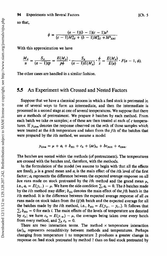
94 Experiments with Several Factors [Ch. 5
so that,
=(a — 1)(b — 1)(c — 1)u2
(c — 1)MÁB + (b — l)MAC +MaABc
With this approximation we have
MA __ SA __ E(MA) , SA , ^ = E(M4) . F(a — 1, ^)u (a — 1)zp p^ (a — 1)E(MA) z E(u)
The other cases are handled in a similar fashion.
5.5 An Experiment with Crossed and Nested Factors
Suppose that we have a chemical process in which a feed stock is pretreated inone of several ways to form an intermediate, and then the intermediate isproceseed in a second stage at one of several temperatures. We suppose that thereare a methods of pretreatment. We prepare b batches by each method. Fromeach batch we take cn samples; n of these are then treated at each of c tempera-tures. If ytikm denotes the response observed on the mth of those samples whichwere treated at the kth temperature and taken from the jth of the batches thatwere prepared by the ith method, we assume a model
Y(lkrn = µ + ai + bl(i) + Ck + (aC)ik + bClk(i) + eilkm•
The batches are nested within the methods (of pretreatment). The temperaturesare crossed with the batches and, therefore, with the methods.
In the formulation of the model (we assume to begin with that all the effectsare fixed), µ is a grand mean and at is the main effect of the ith level of the firstfactor; ai represents the difference between the expected average response on allben runs made on stock pretreated by the ith method and the grand mean µ,i.e., ai = E(y( ...) — µ. We have the side condition li ai = 0. The b batches madeby the ith method may differ; bf(() denotes the main effect of the jth batch in theith method. It is the difference between the expected average response of all cnruns made on stock taken from the (ij)th batch and the expected average for allthe batches made by the ith method, i.e., bf(() = E(yii.. — yj ...). It follows thatIi bt(() = 0 for each 1. The main effects of the levels of temperature are denotedby Ck ; we have ck = E(y..k.) — µ, the averages being taken over every batchfrom every method, and I k Ck = 0.
There are two interaction terms. The method x temperature interaction(ac)ik represents nonadditivity between methods and temperatures. Perhapschanging from temperature 1 to temperature 2 produces a greater change inresponse on feed stock pretreated by method 1 than on feed stock pretreated by
Dow
nloa
ded
12/1
1/12
to 1
29.1
28.2
07.2
42. R
edis
trib
utio
n su
bjec
t to
SIA
M li
cens
e or
cop
yrig
ht; s
ee h
ttp://
ww
w.s
iam
.org
/jour
nals
/ojs
a.ph
p

Sec. 5.5] An Experiment with Crossed and Nested Factors 95
method 2; we have (ac),k = E(yt .k.) — at — ck — µ = E(Yt•k. — Yi--- — Y••k• +y....). The side conditions are 1, (ac) ik = 0, and lk (ac)ik = 0. The temperature xbatch within methods interaction, (bc) ik(j), represents nonadditivity betweentemperatures and different batches made by the same method, and, in essence,accommodates all the scatter between cell means that has not been taken intoaccount so far. The side conditions are k (bc)1k(j) = 0 for each batch, and^1 (bc)fk(i) = 0 for each combination of temperature and method.
There is no AB interaction term. We cannot talk about the main effect ofbatches changing from method to method because batches are nested in methods.A run made at temperature 1 on a stock pretreated by method 1 and a run attemperature 1 on a stock pretreated by method 2 have in common the (possiblyimportant) fact that they were both made at the same temperature. The firstbatch made by method 1 and the first batch made by method 2 do not have abatch factor in common; as we have formulated the experiment there are just bbatches made by each method, and being the first or second batch is just a label.Similarly, there is no ABC interaction. That would have corresponded to an ABinteraction varying from temperature to temperature.
We could now proceed in two ways. We could go back to the linear model,obtain the normal equations, solve them, and derive sums of squares by routinealgebraic procedures. We shall, however, take instead a more practical approach,which can be formalized by considering a set of nested hypotheses.
Our experiment involves ab batches and c temperatures. We can analyze it as atwo-way layout with factors B (batches), C (temperatures), and the usual sumsof squares.
TABLE 5.3ANALYSIS OF VARIANCE
Source SS d.f.
Total Y'Y — C abcn — 1
B T,,../cn—C=SB ab-14 i
C T?k,/abn — C = ST c — 1k
BC T,ƒk./n — C — SB — ST (c — 1)(ab — 1)4 1 k
SBBy subtraction abc(n — 1)
The sum of squares for batches falls into two components, just as in the ordinarynested design.
SA = 1, Ti?../bcn — C is the sum of squares between (or for) methods.SB(A) = lt Ij T,ll ../cn — l i T../bcn is the remainder, and is attributable todifferences between batches made by the same method.
A similar process of subdivision can now be applied to the interaction sum ofsquares. We divide SBC into two components; SAC is the sum of squares for
Dow
nloa
ded
12/1
1/12
to 1
29.1
28.2
07.2
42. R
edis
trib
utio
n su
bjec
t to
SIA
M li
cens
e or
cop
yrig
ht; s
ee h
ttp://
ww
w.s
iam
.org
/jour
nals
/ojs
a.ph
p

96 Experiments with Several Factors [Ch. 5
interaction that we would obtain were we to ignore batches and to consider atwo-way layout with a methods, c temperatures, and bn observations in eachcell. Thus SAC =1,i E, T 2 i . k../bn-1,^ T i 2../bcn —ET2•. k/abn + C witli (a— 1)(b — 1) d.f.; the rest of SABC with a(b — 1) (c — 1) d.f. is the sum of squaresfor interaction between temperature and batches made by the same method (ormore concisely temperature x batches in methods).
In practice, it is more reasonable to regard the b ;( , ) as random variables,uncorrelated (or independent under the normality assumption) with mean zeroand variance oB. The interactions (bc) jk(i) will also be random variables. Supposethat we continue to take methods (A) and temperatures (C) as fixed. The expecta-tions of the sums of squares may be derived by following the same proceduresthat we used for the mixed model in the chapter on the two-way layout. This can,however, be a lengthy process and we shall give in the next section some rules forwriting down the expected mean squares more easily. In our example the table ofexpected mean squares with A and C fixed and B random is
TABLE 5.4
EXPECTED MEAN SQUARES
SS d.f. EMS
SA a — 1 a2 + cn4(A) + bcncASB(A) a(b — 1) a' + CnaB(A)
Sc c — 1 02 + n4c(A) + abnacSAC (a — 1)(c — 1) a2 + naBC(A) + bnaAC
SBc(A) a(b — 1)(c — 1) a2 + n4C(A)
Se abc(n — 1) 02
5.6 General Rules for Sums of Squares and EMS
We present now a set of rules for writing down the form of the model,formulae for the sums of squares, their degrees of freedom, and the expectationsof the mean squares. These rules are also given by Scheffé (1959, pp. 282-289)and by Bennett and Franklin (1954, Sec. 7.6). We shall use the example of thelast section as an illustration.
1. The model contains, in addition to th ° mean and the error term, all maineffects and interactions corresponding to sets of 2, 3,..., factors, except thatthere are no interaction terms containing two factors, one of which is nested inthe other. Thus, in the example there was no AB interaction and no ABCinteraction. The subscripts attached to a term are those corresponding to thefactors appearing in the term. If one of the factors in a term is a nested factor,the letters corresponding to the factors in which it is nested are added in bracketsas subscripts. Thus, we had for the BC in A interaction, (bc);k(,) . The error term iswritten in the form em(, jk) for our present purposes.
Dow
nloa
ded
12/1
1/12
to 1
29.1
28.2
07.2
42. R
edis
trib
utio
n su
bjec
t to
SIA
M li
cens
e or
cop
yrig
ht; s
ee h
ttp://
ww
w.s
iam
.org
/jour
nals
/ojs
a.ph
p
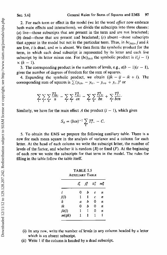
Sec. 5.6] General Rules for Sums of Squares and EMS 97
2. For each term or effect in the model (we let the word effect now embraceboth main effects and interactions), we divide the subscripts into three classes:(a) live—those subscripts that are present in the term and are not bracketed;(b) dead—those that are present and bracketed; (c) absent—those subscriptsthat appear in the model but not in the particular term. Thus, in bc;k( ), j and kare live, i is dead, and m is absent. We then form the symbolic product for theterm, in which Bach dead subscript is represented by its letter and each livesubscript by its letter minus one. For (bc);k(j) the symbolic product is i(j — 1)
x (k — 1).3. The corresponding product in the numbers of levels, e.g., a(b — 1)(c — 1),
gives the number of degrees of freedom for the sum of squares.4. Expanding the symbolic product, we obtain (ijk — ij — ik + i). The
corresponding sum of squares is 1(yi;k. — Yij.• — Yi.k• + y{...) 2 or
Tj TZ T2 TZtik• ti•• i•k• {"'
J ^ n — J cn — 11 bn + { ""
Similarly, we have for the main effect A the product (i — 1), which gives
S,4 = (bcn) 1 T?.. — C.
5. To obtain the EMS we prepare the following auxiliary table. There is arow for each mean square in the analysis of variance and a column for eachletter. At the head of each column we write the subscript letter, the number oflevels of the factor, and whether it is random (R) or fixed (F). At the beginningof each row we write the subscripts for that term in the model. The rules forfilling in the table follow the table itself.
TABLE 5.5AUXILIARY TABLE
iá ja k' mn
i 0 b c n
j(i) 1 1 c nk a b 0 n
ik 0 b 0 njk(i) 1 1 0 nm(ijk) 1 1 1 1
(i) In any row, write the number of levels in any column headed by a letterwhich is an absent subscript.
(ii) Write 1 if the column is headed by a dead subscript.
Dow
nloa
ded
12/1
1/12
to 1
29.1
28.2
07.2
42. R
edis
trib
utio
n su
bjec
t to
SIA
M li
cens
e or
cop
yrig
ht; s
ee h
ttp://
ww
w.s
iam
.org
/jour
nals
/ojs
a.ph
p

98 Experiments with Several Factors [Ch. 5
(iii) In any column corresponding to a random effect, write 1 in the remainingcells.
(iv) In any column corresponding to a fixed effect, write 0 in the remainingcells.
To obtain, for example, E(MA), we cover the ith column. In each row forwhich i is a live or dead subscript, we take the product of the visible numbers andmultiply by the corresponding component of variance. Thus, E(MA) = aa +cnaB(A) + bcnQÁ.
For E(MAC), we cover the i column and the k column and obtain
E(MAC) = a2 + n4C(A) + bnaAC.
5.7 Split-Plot Designs
The experiment that we have just considered is an example of a split-plotdesign. In the agricultural context from which the name is derived, we picture apiece of land divided into several plots, perhaps strips of land or fields. Eachof these plots is then given a single treatment. It is convenient to call these plotswhole plots and to designate the treatments that are applied, one to each wholeplot, as main treatments or levels of a main factor. The whole plots are thensplit into subplots, and one or more subtreatments are applied to each subplot.We might, for example, take several varieties of a erop and sow several fields(whole plots) , with each variety, one variety to a field. Then each field could bedivided into six subplots, and one subplot from each field could be harvestedeach week over a six-week period. The varieties would be the main treatments,and the hervesting times the subtreatments. In comparing the varieties, we musttake into account the field-to-field variation. In comparing harvest times, we cancompare yields within each field. It follows that the main treatments are testedagainst a larger error term (the whole-plot error) than the subtreatments.
In our example the methods of preparing the feedstock are the main treat-ments, the batches are the whole plots, the temperatures are the subtreatments,and the samples drawn from the batches to be run at the various temperaturesare the subplots. It will be recalled that the main effect C is tested againstMBC(A), as is the interaction AC; however, the main effect A is tested againstMB(A) . The most common situation is to have one subplot in each whole plot foreach subtreatment, i.e., n = 1. The main treatments are sometimes said to beconfounded with the whole plots.
The experiment reported by Yates (1937) involving oats and manure(nitrogen), to which we referred in the previous chapter, was a split-plot experi-ment. Six blocks of three plots each were taken, and one plot in each block wassown with each of the three varieties of oats chosen for the experiment. Eachplot was divided into four subplots, one of which was assigned at random toeach level of the nitrogen factor. The four levels were no manure and 0.01, 0.02,
Dow
nloa
ded
12/1
1/12
to 1
29.1
28.2
07.2
42. R
edis
trib
utio
n su
bjec
t to
SIA
M li
cens
e or
cop
yrig
ht; s
ee h
ttp://
ww
w.s
iam
.org
/jour
nals
/ojs
a.ph
p
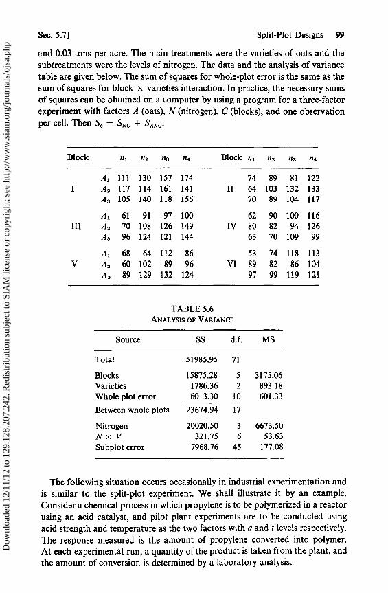
Sec. 5.7] Split-Plot Designs 99
and 0.03 tons per acre. The main treatments were the varieties of oats and thesubtreatments were the levels of nitrogen. The data and the analysis of variancetable are given below. The sum of squares for whole-plot error is the same as thesum of squares for block x varieties interaction. In practice, the necessary sumsof squares can be obtained on a computer by using a program for a three-factorexperiment with factors A (oats), N (nitrogen), C (blocks), and one observationper cel!. Then Se = SNC + SANC•
Block nl n2 n3 n4 Block nl n2 n3 n4
A l 111 130 157 174 74 89 81 122I AZ 117 114 161 141 II 64 103 132 133
A3 105 140 118 156 70 89 104 117
A I 61 91 97 100 62 90 100 116III A2 70 108 126 149 IV 80 82 94 126
A3 96 124 121 144 63 70 109 99
A l 68 64 112 86 53 74 118 113V A2 60 102 89 96 VI 89 82 86 104
A3 89 129 132 124 97 99 119 121
TABLE 5.6ANALYSIS OF VARIANCE
Source SS d.f. MS
Total 51985.95 71
Blocks 15875.28 5 3175.06Varieties 1786.36 2 893.18Whole plot error 6013.30 10 601.33
Between whole plots 23674.94 17
Nitrogen 20020.50 3 6673.50N x V 321.75 6 53.63Subplot error 7968.76 45 177.08
The following situation occurs occasionally in industrial experimentation andis similar to the split-plot experiment. We shall illustrate it by an example.Consider a chemical process in which propylene is to be polymerized in a reactorusing an acid catalyst, and pilot plant experiments are to be conducted usingacid strength and temperature as the two factors with a and t levels respectively.The response measured is the amount of propylene converted into polymer.At each experimental run, a quantity of the product is taken from the plant, andthe amount of conversion is determined by a laboratory analysis.
Dow
nloa
ded
12/1
1/12
to 1
29.1
28.2
07.2
42. R
edis
trib
utio
n su
bjec
t to
SIA
M li
cens
e or
cop
yrig
ht; s
ee h
ttp://
ww
w.s
iam
.org
/jour
nals
/ojs
a.ph
p

100 Experiments-with Several Factors [Ch. 5
Suppose now that it is decided to have four observations at each combinationoflevels of temperature and acid strength. There are two possibilities that come tomind. The first is to make 4 at runs in random order, and then to make an analysisof the product of each run. The second is to make only one run at each combina-tion of levels, but to make four analyses on the product of each run. In eithercase, we end up with four numbers for each cell in the acid-temperature table.
In the first case, the scatter among the numbers in each cell reflects both theprecision of the laboratory analysis and also the `noise' in the whole system.It measures the reproducibility of the results and throws lome light upon thequestion: if we make another run at the ith acid strength and the jth temperaturetomorrow, how well shall we be able to reproduce the results that were obtainedlast week? If y;;,^ denotes the response on the kth run at the ith level of acid andthe jth level of temperature, we could write
Yiik = m + ai + b; + (ab) t; + ei3k + f;k,
where ei;k is a term for the general noise, such as the inability to reproduceexactly the same temperature and perhaps the same acid strength, on differentruns; f;,, is the analytic error. They are independent random variables with zeromeans and variances Qé and of respectively, and V(y;;k) = (aé + af), V(y15.) _(aé + af)/4. The ordinary two-way analysis of variance procedure produces amean square for error s 2 with 3 at d.f. and expectation oé + o, and we havethe situation of the previous chapter.
On the other hand, in the second experimental plan, yi;k denotes the result ofthe kth analysis on the (ij)th run. We write
y„k =m+at +b; +(ab),; + e,; +f;k ,
because for any given i and j, ei». is the same for all four values of k. We haveV(Y;rx) = (a + af) as before, but now V(yt;.) = aé + (o/4).
TheThe sum of squares between duplicate analyses provides an estimate of o
with 3 at degrees of freedom. It does not, however, provide any informationabout o. In consequence, the experimenter who uses the mean square betweenduplicates as his error term in comparing temperatures is using too small anerror estimate. He is using only the analytic variance and is tacitly assuming thathis experimental conditions are perfectly reproducible. This will result in hismaking too many wrong decisions to reject null hypotheses.
How, then, do we test for temperature differences in this case? The answeris that we use for the denominator the mean square for A x T interaction. Weessentially have a two-factor experiment with one run at each combination oflevels; nested within each run are the four analyses. The setup is the same as ifthere were at whole plots, each split into four subplots to which no subtreatmentis applied. If either A or T is fixed, as such factors usually would be, we have thesame problem that we faced in the last chapter when there was one observationper cell and interaction was present. We may sum up with a useful reminder.If, in a factorial experiment, all the main effects and all the interactions turn out
Dow
nloa
ded
12/1
1/12
to 1
29.1
28.2
07.2
42. R
edis
trib
utio
n su
bjec
t to
SIA
M li
cens
e or
cop
yrig
ht; s
ee h
ttp://
ww
w.s
iam
.org
/jour
nals
/ojs
a.ph
p

Sec. 5.8] Split-Split-Plot Designs 101
to be highly significant in the analysis of variance, go back and look at theexperiment again. It may actually be a split-plot situation, and you may betesting everything against the repeatability of a chemical balance in the hands ofan expert technician!
The following example illustrates a slightly different aspect of the topic thathas just been discussed. Chanda, et al. (1952) fed carotene to goats and cows overconsecutive two-day periods and used two methods to measure the digestibilityof the carotene. The data shown are for four goats over five periods. In each cell,the first number given is the apparent digestibility measured by method 1. Thesecond number is the measurement by method 2.
The goat-period combinations can be regarded as 4 x 5 = 20 whole plots.Each whole plot is split into two subplots. Method 1 is applied to one subplotand method 2 to the other. The goat and period main effects are tested againstthe mean square for goat x period interaction. The M x G x P mean squareis used to test M, M x G and M x P. It wilt be noted that if the M x G x Pmean square had been used to test G and P, each of those effects would have beendeemed significant.
Periods
Goats I II III IV V
Anna 75.1, 75.2 69.0, 63.5 74.3, 80.7 51.2, 46.7 72.6, 71.0Betty 65.4, 62.7 63.3, 61.2 59.4, 65.3 62.9, 62.1 63.8, 63.1Bluebell 61.9, 60.1 57.7, 59.6 74.4, 75.8 62.9, 55.3 54.3, 58.3Diana 69.4, 70.1 60.7, 57.0 57.0, 54.5 56.6, 49.5 64.3, 63.3
TABLE 5.7
ANALYSIS OF VARIANCE
Source SS d.f. MS F values
Methods (M) 11.03 1 11.03 2.28Goats (G) 328.44 3 109.48 1.20Periods (P) 760.13 4 190.03 2.09M x G 10.23 3 3.41 0.71M x P 67.27 4 16.82 3.48G x P 1090.77 12 90.90 18.82M x G x P 57.99 12 4.83Total 2325.86 39
5.8 Split-Split-Plot Designs
In some experimental situations, further subdivision of the subplots is used. Anexample is the experiment conducted by Tandon (1949) to investigate the responseof flax to various rates of application and formulations of the herbicide 2,4-D.
Dow
nloa
ded
12/1
1/12
to 1
29.1
28.2
07.2
42. R
edis
trib
utio
n su
bjec
t to
SIA
M li
cens
e or
cop
yrig
ht; s
ee h
ttp://
ww
w.s
iam
.org
/jour
nals
/ojs
a.ph
p

102 Experiments with Several Factors [Ch. 5
He chose seven varieties of flax with three formulations of 2,4-D and fourrates of application. There were four replications in the experiment. Eachreplicate involved twelve blocks, each with seven plots, so that there were 336plots altogether. One plot in each block was sown with each variety of flax.The three formulations of 2,4-D were made up, and four blocks in each replicatewere assigned to each formulation. The 2,4-D was then applied to one of theblocks at the lowest rate, to another at the second rate, and so on. In any block,each of the seven plots received the same formulation at the same rate. In thesplit-split-plot context there are twelve whole plots with formulations as thewhole-plot factor. Each of the whole plots is split into four subplots (the blocks),with rates of application as the subplot factor. Each subplot is split into sevensub-subplots with flax as the sub-subplot factor. The sources of variation andthe degrees of freedom for their sums of squares are
Replications 3F = formulations 2Reps x F= Error (a) 6R = Rates 3R x F 6Error (b) 27V 6V x F 12VxR 18VxRxF 36Error (c) 216
He obtained his error (b) term for testing R and R x F by pooling the sums ofsquares for reps x R and reps x R x F. The sum of squares for error (c) isobtained by subtraction and consists of everything that has not been usedalready. As usual, it is assumed that replications do not interact with any of theother factors.
5.9 Computer Programs
The analysis of variance calculations for all these designs can readily be carriedout on a computer. It is relatively easy to write a program for a completefactorial design with one observation per cell, and most computer centers haveone available. It is not necessary to write a special program for each design whensome factors are nested or when there are split plots. A few examples will sufficeto show how the simple program can be used for the more complex designs withthe help of a few additions with pencil and paper. We have already mentionedthis in regard to the Yates experiment with oats and manure.
1. A two-factor design with r observations per cell. We have merely to pretendto ourselves that there are three factors. If y,fk is the kth observation at the ith
Dow
nloa
ded
12/1
1/12
to 1
29.1
28.2
07.2
42. R
edis
trib
utio
n su
bjec
t to
SIA
M li
cens
e or
cop
yrig
ht; s
ee h
ttp://
ww
w.s
iam
.org
/jour
nals
/ojs
a.ph
p
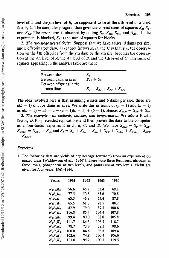
Exercises 103
level of A and the jth level of B, we suppose it to be at the k th level of a thirdfactor, C. The computer program then gives the correct sums of squares SA, SB ,
and SAB . The error term is obtained by adding Sc, S c, SBC, and SABC. If theexperiment is blocked, Sc is the sum of squares for blocks.
2. The two-stage nested design. Suppose that we have s sires, d dams per sire,and n offspring per dam. Take three factors A, B, and C so that y ijk, the observa-tion on the kth offspring from the jth dam by the ith sire, becomes the observa-tion at the i th level of A, the j th level of B, and the kth level of C. The sums ofsquares appearing in the analysis table are then:
Between sires SA
Between dams in sires SAB + SB
Between offspring in thesame litter Sc + SAC + SBC + SABC.
The idea involved here is that assuming a sires and b dams per sire, there area(b - 1) d.f. for dams in sires. We write this in terms of (a - 1) and (b - 1)as a(b - 1) = ab - a = (a - 1)(b - 1) + (b - 1). Hence, SB(A) = SAB + SB .
3. The example with methods, batches, and temperatures. We add a fourthfactor, D, for pretended replications and then present the data to the computeras a four-factor experiment in A, B, C, and D. We have SB(A) = SB + SAB ,
SBC(A) = SABC + SBC and Se = SD + SAD + SBD + SCD + SABD + SACD + SBCD
+ SABCD-
Exercises
1. The following data are yields of dry herbage (cwt/acre) from an experiment ongrazed grass [Widdowson et al., (1966)]. There were three fertilizers, nitrogen atthree levels, phosphorus at two levels, and potassium at two levels. Yields aregiven for four years, 1961-1964.
Years 1961 1962 1963 1964
NoPoKo 56.6 46.7 62.4 69.1N0P1K0 77.5 50.8 65.6 70.8N0P0K1 63.3 46.8 65.4 87.8N0P1K1 65.5 61.8 78.5 88.7N1P0K0 82.9 79.0 89.8 100.6N,P1Ko 116.8 85.4 104.4 107.8N,PoKi 99.4 80.0 88.0 105.8N1P1K1 111.7 84.3 106.2 118.7N2PoKo 78.7 73.3 78.2 98.6N2P1Ko 100.0 84.6 98.8 109.4N2PoK1 102.6 74.8 100.4 106.0N2P1K1 123.8 95.2 100.7 119.5D
ownl
oade
d 12
/11/
12 to
129
.128
.207
.242
. Red
istr
ibut
ion
subj
ect t
o SI
AM
lice
nse
or c
opyr
ight
; see
http
://w
ww
.sia
m.o
rg/jo
urna
ls/o
jsa.
php
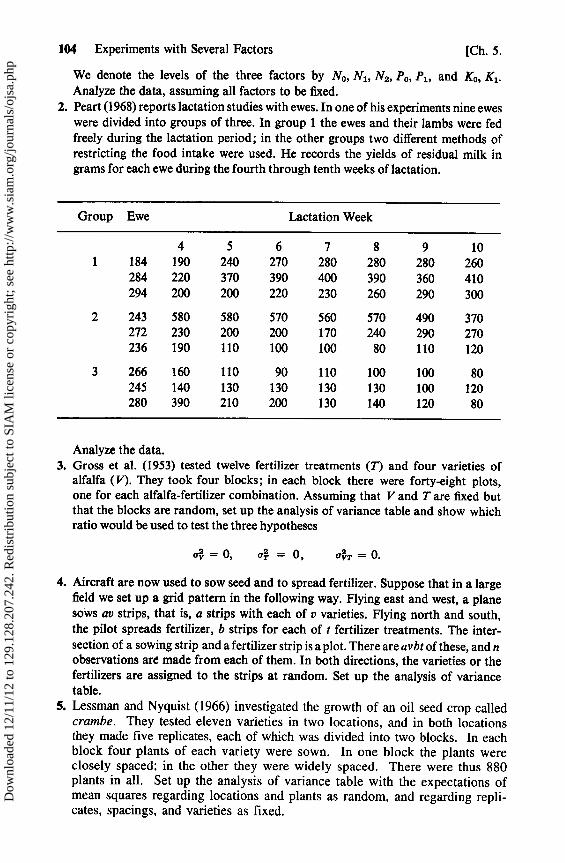
104 Experiments with Several Factors [Ch. 5.
We denote the levels of the three factors by No , Nl , N2 , Po, Pl, and Ko, K.Analyze the data, assuming all factors to be fixed.
2. Peart (1968) reports lactation studies with ewes. In one of his experiments nine eweswere divided into groups of three. In group 1 the ewes and their lambs were fedfreely during the lactation period; in the other groups two different methods ofrestricting the food intake were used. He records the yields of residual milk ingrams for each ewe during the fourth through tenth weeks of lactation.
Group Ewe Lactation Week
4 5 6 7 8 9 101 184 190 240 270 280 280 280 260
284 220 370 390 400 390 360 410294 200 200 220 230 260 290 300
2 243 580 580 570 560 570 490 370272 230 200 200 170 240 290 270236 190 110 100 100 80 110 120
3 266 160 110 90 110 100 100 80245 140 130 130 130 130 100 120280 390 210 200 130 140 120 80
Analyze the data.3. Gross et al. (1953) tested twelve fertilizer treatments (T) and four variaties of
alfalfa (V). They took four blocks; in each block there were forty-eight plots,one for each alfalfa-fertilizer combination. Assuming that V and T are fixed butthat the blocks are random, set up the analysis of variance table and show whichratio would be used to test the three hypotheses
4 = 0, 4 = 0, QVT = 0 .
4. Aircraft are now used to sow seed and to spread fertilizer. Suppose that in a largefield we set up a grid pattern in the following way. Flying east and west, a planesows av strips, that is, a strips with each of v varieties. Flying north and south,the pilot spreads fertilizer, b strips for each of t fertilizer treatments. The inter-section of a sowing strip and a fertilizer strip is a plot. There are avbt of these, and nobservations are made from each of them. In both directions, the varieties or thefertilizers are assigned to the strips at random. Set up the analysis of variancetable.
5. Lessman and Nyquist (1966) investigated the growth of an oil seed erop calledcrambe. They tested eleven varieties in two locations, and in both locationsthey made five replicates, each of which was divided into two blocks. In eachblock four plants of each variety were sown. In one block the plants wereclosely spaced; in the other they were widely spaced. There were thus 880plants in all. Set up the analysis of variance table with the expectations ofmean squares regarding locations and plants as random, and regarding repli-cates, spacings, and varieties as fixed.
Dow
nloa
ded
12/1
1/12
to 1
29.1
28.2
07.2
42. R
edis
trib
utio
n su
bjec
t to
SIA
M li
cens
e or
cop
yrig
ht; s
ee h
ttp://
ww
w.s
iam
.org
/jour
nals
/ojs
a.ph
p
CHAPTER 6
Latin SquareDesigns
In Chapter 3 we discussed the experiment in which five gasolines were tested incars and their road octane numbers observed. Four observations were to be madeon each gasoline. We began with the completely randomized experiment inwhich twenty cars were chosen and four of them were assigned by some randomprocedure to each gasoline. Later in the chapter we introduced the randomizedcomplete block design. There we took only four cars. Each gasoline was testedonce in each car. The car differences canceled out when gasolines were compared,and the precision of the experiment for comparing gasolines was thereby im-proved. In an agricultural experiment, where we have reason to think thatthe land becomes more fertile as we move from north to south, suitable blocksmight be strips of land running from east to west with one plot per block foreach of the treatments or varieties being tested. In either case, the treatmentsare randomized within the blocks. In the case of the gasolines, the order inwhich they are to be tested is chosen randomly for each car; the agronomistassigns the plots within each block at random to the different varieties.
Let us change the experiment slightly so that the response we observe is therate of consumption in miles per gallon, with the added restriction that eachcar can only make one run, i.e., test one gasoline, per day. It may be that condi-tions vary during the working week. Perhaps early in the week the weather iscold and damp, but as the week wears on the sun appears and the weatherbecomes warmer and drier. This could conceivably have some influence upon theperformance of the cars and upon the ratings that they give the gasolines.Unless something is done about it, this day-to-day variation may ruin the wholeexperiment. In an extreme situation suppose that all the cars use only gasoline Aon Monday, which is bright and Bunny, and that all the cars make their test of
105
Dow
nloa
ded
12/1
1/12
to 1
29.1
28.2
07.2
42. R
edis
trib
utio
n su
bjec
t to
SIA
M li
cens
e or
cop
yrig
ht; s
ee h
ttp://
ww
w.s
iam
.org
/jour
nals
/ojs
a.ph
p
106 Latin Square Designs [Ch. 6
gasoline B on Friday when the temperature is twenty degrees lower and it israining steadily. We might gain some insight into the relative merits of the carsused under a variety of conditions, but we should not be able to tell whether ahigher rating in miles per gallon of gasoline A over gasoline B results from thedifferences between the gasolines or from the differences in the weather. We wereable to increase the precision of the earlier experiment when we removed the careffects by blocking. We should be able to make a further improvement in theprecision if we could balance out the day effects. This calls for an experimentalscheme in which each gasoline is tested once in each car and once on each day(or in each position in the block). This cannot be done with five days and onlyfour observations on each gasoline. Suppose that we allow ourselves a fifth car.We can then use a Latin square design for the experiment.
A Latin square of side p, or a p x p Latin square, is an arrangement of pletters, each repeated p times, in a square array of side p in such a manner thateach letter appears exactly once in each row and in each column. Four Latinsquares of side five are
ABCDE ABCDE ABCDE ABCDEBCDEA CDEAB DEABC EABCDCDEAB EABCD BCDEA DEABCDEABC BCDEA EABCD CDEABEABCD DEABC CDEAB BCDEA.
Suppose that we were to use the first of these squares and to let the rows denotethe cars, the columns the days, and the letters the gasolines. Then, on thesecond day (column 2) the first car (row 1) uses gasoline B, the second car (row 2)uses gasoline C, and so on. As we have written it, this square has a more system-atic pattern than is needed or is desirable since for every car the gasolines followone another in alphabetical order. In practice, the experimenten should assignthe cars at random to the rows and the days at random to the columns (i.e., orderthe columns by a random procedure).
6.1 Analysis
We assume a completely additive model; more will be said about this assump-tion later. Let Yifk denote the observation corresponding to the kth letter in theith row and the jth column, if there is one, i.e., to the observation on the kthgasoline in the ith car on the jth day where 1 < i, j, k < p. The row, column,and letter effects are denoted by pi , yf, and Tk , respectively, and for the presentwe assume them to be fixed effects; µ is the grand mean and e1 ik is the randomerror with the usual assumptions about homoscedasticity and normality. We thenhave
Yiik = 1 t + Pi + Í'! + Tk + eilk•
Dow
nloa
ded
12/1
1/12
to 1
29.1
28.2
07.2
42. R
edis
trib
utio
n su
bjec
t to
SIA
M li
cens
e or
cop
yrig
ht; s
ee h
ttp://
ww
w.s
iam
.org
/jour
nals
/ojs
a.ph
p

Sec. 6.1] Analysis 107
We shall denote the row, column, and letter totals by Ti.., T. 1., and T..k, and thecorresponding means by y,.., y.,., Y..k; the grand mean will be denoted by y....In addition to the side conditions 1, p t = 0 and 1f y, = 0, we impose thecondition Ik Tk = 0 . The normai equations are then easily solved, and the leastsquares estimates of the parameters are
^ = Y..., Pc = Y:.. — Y..., Yr = Y. i . — Y... 1 fk = Y..k — y....
The analysis of variance table follows. Under normality, the sums of squaresare distributed independently. The appropriate test statistics for the hypothesesof no row effects, no column effects, or no letter effects are the ratios of thecorresponding mean squares to the mean square for error. Under the nullhypotheses, these ratios will each have the tentral F distribution with (p — 1)and (p — 1)(p — 2) degrees of freedom. If, for example, the row effects arerandom variables with mean zero and variance 4, we use the same breakdowninto sums of squares. The expected value of the mean square for rows is thena2 + p4R.
TABLE 6.1ANALYSIS OF VARIANCE
Source SS d.f. EMS
Total 1, I J I k Y4lk — C p2 —1Rows p - 1 1, T,. — C p — 1 a2 + p 1, p?/(p — 1 )Columns p -1 Ii T.J. — C p —1 a2 + p Ii yf/(p — 1)Letters p-1 Ik T.?k — C p — 1 oz + p Ik Tkl(p — 1)Error By subtraction (p — 1)(p — 2) 02
In the example of the gasoline experiment, the purpose of using the Latinsquare design was to improve the precision of the gasoline comparisons byeliminating the car and day effects. In agricultural experiments we could usesuch designs to eliminate fertility trends in two perpendicular directions, east-west as well as north-south; this was the context in which they were first intro-duced, and they are sometimes called designs for the elimination of two-wayheterogeneity. It is customary to refer to the three classifications as rows,columns, and treatments. The requirement that there should be the samenumber of rows and columns as there are treatments can present a difficulty, andalternative designs which involve incomplete blocks can be used. That, however,is a topic for later discussion.
The Latin square can also be used in factorial experiments. A completefactorial experiment with three factors each at five levels, which we may call a53 experiment, calls for 125 points. If we take one of the Latin squares we canlet the rows denote the levels of the first factor, the columns the levels of thesecond factor, and the letters the levels of the third factor. Then we have a set of
Dow
nloa
ded
12/1
1/12
to 1
29.1
28.2
07.2
42. R
edis
trib
utio
n su
bjec
t to
SIA
M li
cens
e or
cop
yrig
ht; s
ee h
ttp://
ww
w.s
iam
.org
/jour
nals
/ojs
a.ph
p
108 Latin Square Designs [Ch. 6
twenty-five out of the 125 points with the property that for any two of thefactors each level of one appears exactly once at each level of the other. In thegeneral case we have a (l/p)th fraction of the complete factorial design. Thisreduction in the number of points can be very attractive. When p = 5, itrepresents an 80 per cent reduction in the number of observations that have to bemade. The additive model that we have assumed may be rewritten
Yi1k= N+ai +Ni+Yk+etlk,
where Y,;k is the observation, if any, made at the ith level of the first factor, thejth level of the second factor, and the kth level of the third factor, and ai , PJ, andYk are the corresponding main effects. The analysis follows the same lines, andwe have tests for the main effects of the factors. Contrasts may be tested by anyof the usual multiple comparison methods. The reduction in the number ofpoints obliges us to assume in our model that there are no interactions. Thisrestriction may be serious; it is discussed in the next section.
This type of fractional factorial design may become necessary because ofbudget restrictions. It may also be necessary if time is one of the factors, as it isfor the dairy cattle and crop rotation experiments that we shall discuss later inthis chapter. Consider, for example, an experiment to investigate the consump-tion of lubricating oil in buses. Suppose that there are three brands of oil, X, Y,and Z. We could take three groups of new buses (A, B, and C) and conduct atest over three months (I, II, and III), in which case an observation would showthe average consumption of a test oil by a group of buses in a month. We mighthave group A use oil X for the first month, followed by oil Y for the secondmonth, and oil Z for the third month. We cannot use two oils simultaneously inthe same bus and so, even though we might think of a factorial experiment in thethree factors (oils, groups, and months, each at three levels), we can observe onlyone of the three points AIX, AI Y, and AIZ. We are obliged to use one-thirdfractions of the three-factor design, and the use of one or more Latin squareswould be appropriate.
6.2 Limitations of the Model
In the analysis of the Latin square design we assumed a completely additivemodel with no interaction terms. As long as this model is justified, there is noproblem about the validity of the analysis. However, if there is, for example,interaction between rows and columns, this interaction biases the estimates ofthe treatment effects. This difficulty can be illustrated in the gasoline experimentthat has just been discussed. Using the first square, suppose that there is indeeda row-column interaction (py)j to be added to the model. Over the set of rowsand the set of columns we have (py)ij = 0 for each j and Lf (py)u = 0 foreach i. These side conditions ensure that the interactions cancel out of E(fc).
Dow
nloa
ded
12/1
1/12
to 1
29.1
28.2
07.2
42. R
edis
trib
utio
n su
bjec
t to
SIA
M li
cens
e or
cop
yrig
ht; s
ee h
ttp://
ww
w.s
iam
.org
/jour
nals
/ojs
a.ph
p

Sec. 6.2] Limitations of the Model 109
Let us consider, in particular, the gasoline that had been labeled treatment A.We shall use subscripts 1, 2, 3, 4, and 5 for gasolines A, B, C, D, and E. We thenhave
5 5
T.. 1 = 5µ + 1 pi + yj + 5,r1 + (py)t> + 5e.. 1i=1 j=1 4 j
The terms 1f yf and 1i pi vanish by virtue of the side conditions but the inter-action terms that are actually involved are only a subset of the p2 possible (py)interactions, and there is no reason to expect them to vanish. They remain as anunwanted and unknown nuisance. In this case the bias is
(py)11 + (PY)25 + (py)34 + (py)43 + (py)52•
We might have chosen to label the gasoline in question treatment B rather thantreatment A, in which case the bias would have been
(PY)12 + (py)21 + (py)35 + (py)44 + (py)53,
or we might have retained the label A and used the second square, in which casethe bias would have been
(Py)11 + (PY)24 + (PY)32 + (py)45 + (py)53,
and so on. Thus, summing, or averaging, over all the labels and over all foursquares, it can be seen that the bias cancels out. In any particular square and forany particular label there is a bias, but over the whole set it averages out. Thisleads to the argument that the experimenter should choose his Latin square atrandom from the set of all squares of side p and, having done so, assign theletters at random to the treatments; by this procedure he would eliminate theunwanted bias.
It is, alas, cold comfort to the experimenter, who has for his particular experi-ment one particular square, to know that if he could repeat his experimentmany times using randomly selected squares, the bias would on the averagedisappear and to that extent, even in the presence of row-column interactions,treatment differences would be estimable. He is saddled with the single square thathas been chosen, and his results are conditional upon the choice of that square.
Nor is the error term free from bias. Scheffé (1959) shows that in the fixedeffects case the expectation of the mean square for error contains a term involvingthe interactions, which is nonnegative and may or may not be appreciable.The problem of bias in Latin squares was first noted by Neyman et al. (1935).Wilk and Kempthorne (1957) consider a random effects model in a similar way.In their model, rows, columns, and treatments are all considered as randomeffects; they show that in this case, too, the mean squares for rows, columns,treatments, and error are all biased if the simple additive model does not hold.Kempthorne (1952) and Scheffé (1959) discuss randomization models as alter-natives to the models presented here.
Dow
nloa
ded
12/1
1/12
to 1
29.1
28.2
07.2
42. R
edis
trib
utio
n su
bjec
t to
SIA
M li
cens
e or
cop
yrig
ht; s
ee h
ttp://
ww
w.s
iam
.org
/jour
nals
/ojs
a.ph
p

110 Latin Square Designs [Ch. 6
6.3 Graeco-Latin Squares
Suppose that we take a Latin square and superimpose upon it a second squarewith the treatments denoted by Greek letters. If the two squares have the prop-erty that each Latin letter coincides exactly once with each Greek letter whenthe squares are superimposed, then they are said to be orthogonal. The com-bined squares are said to form a Graeco-Latin square. Adding a third squareorthogonal to each of the others gives a hyper-Graeco-Latin square. The foursquares of side five that were given at the beginning of this chapter form a set ofmutually orthogonal squares.
Graeco-Latin squares can be used to provide designs for four factors (rows,columns, Latin letters, Greek letters), each at p levels in p 2 runs. Thus, in ourexample of the gasoline experiment, a fourth factor, drivers, might be introducedby combining the first two squares and using the Greek letters to represent thedrivers:
Aa Bfl Cy DS Ee
By C8 De Ea AP
Ce Da ES Ay B8
Dfl Ey AS Be Ca
ES Ae Ba Cp Dy
On the fourth day of the test, driver a uses gasoline E in car 2, driver P usesgasoline C in car 5, driver y uses gasoline A in car 3, driver 8 uses gasoline D incar 1, and driver e uses gasoline B in car 4. The analysis with the additive modelfollows the same procedure as the analysis of the Latin square design. There is anadditional sum of squares for Greek letters with (p — 1) degrees of freedom andthere are only (p — 1) (p — 3) degrees of freedom for error.
Indeed, we could go further by having five different test courses and by havingeach of the cars driven over a different course each day. Courses could be addedas a fifth factor by incorporating the third Latin square and using lower caseletters a, b, c, d, and e to denote the five courses. That would leave only (p — 1)x (p — 4) = 4 degrees of freedom for error. A sixth factor, perhaps predeter-mined average driving speeds, could be added by incorporating the fourthsquare and using Arabic numerals to denote the levels. There would then be nodegrees of freedom left for error, and, without some prior estimate of thevariance, testing hypotheses would present some difliculties. However, there is achance that perhaps one or two of the main effects might stand out much largerthan the others, which would point out the way to further experimentation. Itmay be observed that if the experiment is going to need five cars, each on all-daytrips, we are certainly going to need at least five drivers. It does not, however,follow that we are obliged to add drivers as a fourth factor and to use a Graeco-Latin square. It depends upon the nature of the interest in the cars and drivers.
Dow
nloa
ded
12/1
1/12
to 1
29.1
28.2
07.2
42. R
edis
trib
utio
n su
bjec
t to
SIA
M li
cens
e or
cop
yrig
ht; s
ee h
ttp://
ww
w.s
iam
.org
/jour
nals
/ojs
a.ph
p

Sec. 6.4] Sets of Orthogonal Latin Squares 111
If we wish to investigate whether there are car differences and whether there aredriver differences, then we must add drivers as a fourth factor and, unless we areprepared to increase the size of the experiment, the Graeco-Latin square wouldbe appropriate, with only eight degrees of freedom for error. However, if we areinterested only in comparing gasolines, and thus regard car and driver differ-ences, if any, as nuisances to be eliminated, we should be better advised to usethe same driver with the same car throughout the experiment. Then the drivereffects and the car effects would both be absorbed in the row effects, whichwould now denote car-driver combinations, and we should have twelve degreesof freedom for error.
The Graeco-Latin squares and the hyper-Graeco-Latin squares are, like theLatin squares, fractional factorial designs. The Graeco-Latin square is a (1/p 2)fraction of the p4 design, i.e., the factorial with four factors, each at p levels.The square with no degrees of freedom left for error is a (1 /p' -1) fraction of thepP+l factorial. Such a fraction, in which every degree of freedom is used forestimation, is said to be a saturated fraction.
This ability to add extra factors without increasing the size of the experimentappears attractive on the surface, but the experimenter should note that notonly does the number of degrees of freedom for error diminish as more factorsare added, but also the problems with nonadditivity, which are so bothersomein the Latin square layout, become even more troublesome. Graeco-Latinsquares exist whenever p is a prime, or a power of a prime, and for some othervalues. Complete sets of p — 1 mutually orthogonal squares for p = 3, 4, 5, 7, 8,and 9 are given in the Fisher and Yates tables.
6.4 Sets of Orthogonal Latin Squares
Now we present a method, due to Bose (1938), of obtaining sets of p — 1mutually orthogonal Latin squares of side p when p is a prime or a power of aprime. We associate each of the treatments with an element of the Galois fieldof p = s n elements, GF(s n), in a one-to-one correspondence. The elements ofthe field are ordered as g o = 0, g1 = 1, g2 = x, g3 = x2, ... , gp _ 1 = X - 2
where x is a primitive element of the field, i.e., x is an element such that xp -1 = 1and there is no other power x° = 1, 0 < q < p. Then the addition table formsa Latin square, and the other squares are obtained by rotating cyclically allthe rows except the first.
EXAMPLE 1. p = 4. GF(22) has elements 0, 1, x, and 1 + x. Arithmetic iscarried out mod 2, and x is a primitive element. The irreducible polynomial ofthe second degree in the field is x 2 + x + 1. Equating this polynomial to zero,and recalling that —1 - 1 (mod 2), we have x2 = 1 + x, and x3 = x + x2 = 1.In the addition table, the first row consists of the elements 0, 1, x, and 1 + x;
Dow
nloa
ded
12/1
1/12
to 1
29.1
28.2
07.2
42. R
edis
trib
utio
n su
bjec
t to
SIA
M li
cens
e or
cop
yrig
ht; s
ee h
ttp://
ww
w.s
iam
.org
/jour
nals
/ojs
a.ph
p

112 Latin Square Designs [Ch. 6
the second row is 0 + 1 = 1, 1 + 1 = 0, x + 1 = 1 + x, 1 + x + 1 = x; andso on. The complete table is
0 1 x l+x1 0 l+ x xx 1+x 0 11+x x 1 0
Writing A, B, C, and D for the elements 0, 1, x, and 1 + x, respectively, androtating the rows other than the first cyclically, we obtain the following threesquares. They form a mutually orthogonal set of squares of side 4.
ABCD ABCD ABCD
BADC CDAB DCBA
CDAB DCBA BADC
DCBA BADC CDAB
The first row of each square is the same. The second row of the second squareis the same as the third row of the first square. The third row of the second squareis the fourth row of the first square. The last row of the second square is thesecond row of the first square. The third square is obtained from the secondsquare in the same way.
We now show that Bose's method is valid in the general case. We define the ithsquare of the set to be the square that has gi = xi -1 as the first element of thesecond row. The first element of the (m + 1)th row is gi .xm -1 = gigm . We writethe ith square, therefore, as
0 1 ... gP-1
gi g+1 ... gi + gP -1
gig2 gig2 + 1 ... gig2 + gP-1
gigP-1 gigP-1 + 1 ... gigp-1 + gP-1
We need to establish two properties:
Property 1. Such a square is a Latin square.
PROOF. Suppose that it is not a Latin square and that two of the elements thatappear in the (q + 1)th row are identical, i.e., for some pair t, u, (t # u), gigq +gt = gig, + g,. This implies gi = g, which is false because the elements of thefield are distinct. u
Dow
nloa
ded
12/1
1/12
to 1
29.1
28.2
07.2
42. R
edis
trib
utio
n su
bjec
t to
SIA
M li
cens
e or
cop
yrig
ht; s
ee h
ttp://
ww
w.s
iam
.org
/jour
nals
/ojs
a.ph
p

Sec. 6.4] Sets of Orthogonal Latin Squares 113
Property 2. The squares in the set are mutually orthogonal.
PROOF. Suppose that the ith and jth squares are not orthogonal. This meansthat when the jth square is superimposed on the ith square, one pair of elementsoccurs together in two of the cells. Suppose that these cells are in the (q + 1)throw and the (t + 1)th column and in the (r + 1)th row and the (u + l)thcolumn where q r, t # u. In these two cells the elements of the i th squarecoincide to give
gjgq + gt = g{g. + g.,
and the elements of the jth square coincide to give
gjgq + gt = grg. + g„•
Subtracting, we have (g{ — gj)gq = (g{ — gf)g,. This would imply that eitherg{ = g. or gQ = g, in contradiction. E
This method was also presented by Stevens (1939). In his paper, Stevenspoints out that the orthogonal set for p = 9 given by Yates in the 1948 editionof the Fisher and Yates tables is not isomorphic to the set that Stevens himselfobtained using Galois fields, i.e., the one set cannot be obtained from the otherby a reassignment of the letters to the treatments.
It is easily verified that if p is a prime, rather than sn where n > 1, it is notnecessary to find a primitive element of GF(p) in order to obtain an initialsquare. Bose points out that we can, instead, work with the residue classes(mod p) and write the rows of the initial square in any order we wish.
EXAMPLE 2. p = 5. We shall now give two possible initial squares of side 5.The first of these is derived by the previous procedure. The elements of GF(5)are 0, 1, 2, 3, and 4. Arithmetic is mod 5 and x = 2 is a primitive element. Itspowers are x2 = 4, x 3 = 3, and x4 = 1. The first row (and column) of theaddition table as we write it to form the initial square is, therefore, 0, 1, 2, 4,and 3.
The second initial square is obtained by writing the residue classes (mod 5) inthe usual order 0, 1, 2, 3, and 4 and forming the addition table. The ith squareof this set is obtained by re-ordering the rows of the initial square so that thefirst column is 0, i, 2i, 3i,.... Writing A, B, C, D, and E for 0, 1, 2, 3, and 4,respectively, produces the set of mutually orthogonal squares of side 5 given atthe beginning of the chapter.
01243 0123412304 1234023410 2340140132 3401234021 40123
Dow
nloa
ded
12/1
1/12
to 1
29.1
28.2
07.2
42. R
edis
trib
utio
n su
bjec
t to
SIA
M li
cens
e or
cop
yrig
ht; s
ee h
ttp://
ww
w.s
iam
.org
/jour
nals
/ojs
a.ph
p
114 Latin Square Designs [Ch. 6
There are no similar methods of obtaining sets of p — 1 mutually orthogonalsquares of side p when p is not a prime or a power of a prime. Indeed, Bruck andRyser (1949) have shown that if p - 1 or 2 (mod 4), and if the square free partof p contains at least one prime factor q - 3 (mod 4), then no orthogonal set ofp — 1 squares exists. It had been conjectured by Euler that if p = 2 (mod 4),there did not exist a pair of orthogonal squares, and this conjecture was verifiedfor the case p = 6 by Tarry (1901). However, Bose, Shrikhande, and Parker, in aseries of papers, have shown that if p - 2 (mod 4) and p > 6, a pair of orthog-onal squares always exists. A pair of orthogonal squares found by them (1960)for p = 10 follows.
A pair of orthogonal Latin squares of side 10.
00 47 18 76 29 93 85 34 61 5286 11 57 28 70 39 94 45 02 6395 80 22 67 38 71 49 56 13 0459 96 81 33 07 48 72 60 24 1573 69 90 82 44 17 58 01 35 2668 74 09 91 83 55 27 12 46 3037 08 75 19 92 84 66 23 50 4114 25 36 40 51 62 03 77 88 9921 32 43 54 65 06 10 89 97 7842 53 64 05 16 20 31 98 79 87
6.5 Experiments Involving Several Squares
The single Latin square contains only p observations with each treatment.If the experimenter wishes to have more replications of each treatment, he mayfind it desirable to use several squares. The following analysis is valid whether thesquares chosen are the same or different. We suppose that there are s squares.
Let Yhifk denote the observation, if there is one, made upon the kth treatmentin the ith row and the jth column of the hth square. The model taken is
Yh(Jk = 9 + 7rh + Pi(h) + y1(h) + Tk + (ITT)hk + ehilk,
where 7rh is the effect of the hth square and (1r r)hk represents the interactionbetween squares and treatments; P, (h) and yi(h) are the row and column effects inthe hth square. The side conditions on the parameters are h 7rh = 0, -y^ P((h) = 0for each h, Ii y f(h) = 0 for each h, Ik rk = 0, (ITT)hk = 0 for each h, andlh (1TT)hk = 0 for each k.
With these side conditions, the estimates of the parameters are
^L = Y...., 17h = Yh... — Y...., fk = Y...k — Y....,
Pi(h) = Y,a.. — Yh•••, y!(h) = Yh•!• — Yn...,
()hk = Yh..k — Yh... — Y...k + Y.....
Dow
nloa
ded
12/1
1/12
to 1
29.1
28.2
07.2
42. R
edis
trib
utio
n su
bjec
t to
SIA
M li
cens
e or
cop
yrig
ht; s
ee h
ttp://
ww
w.s
iam
.org
/jour
nals
/ojs
a.ph
p

Sec. 6.6] Change-Over Designs 115
The analysis of variance table is
TABLE 6.2ANALYSIS OF VARIANCE
Source SS d.f.
Total lh Gt G1 Gk Yhjk — C spa — 1Squares lh T,a.../p2 — C = Ss s — 1Treatments Ik T.?.k/(SP) — C = St p — 1T x S >hIkTh•k/p—C —S8 —S, (s-1)(p-1)Rows in squares Tnt.. /p — lh Th ../pa s(p — 1)Columns in squares lh 21 T,? f.lP — Ih T.../p 2 s(p — 1)Residual By subtraction s(p — l)(p — 2)
6.6 Change-Over Designs
In the previous section we considered the s squares as separate squares. Wemay also consider them as being arranged in a rectangle with p rows and spcolumns. This situation typically occurs when time, in the form of periods, is afactor in the experiment. In experiments with dairy cattle, for example, we maytestp treatments (such as kinds of feed) overp periods using sp cows. Each cow haseach feed for one of the p periods, and the schedules are arranged so that duringeach period each feed is given to s cows. In the rectangular arrangement, theperiods correspond to rows and the cows to columns. Alternatively, we mayhave p subjects receiving p treatments over sp periods; each subject receives eachtreatment for s of the periods; during each period each of the treatments is usedon one of the subjects. In either case, we may let
Ytik = µ + Pt + y1 + T k + etik,
where 1 <i<p,1 <j< sp, and 1 <k<p.
TABLE 6.3ANALYSIS OF VARIANCE
Source SS d.f. EMS
Total 21211k ytlk — C spe —Rows 1, T./(sp) — C p — 1 02 + sp I, pi l(p — 1)Columns T. f /p — C sp — 1 02 + p 1, y2 /(sp — 1)Treatments Ik T.?k/(sp) — C p — 1 02 + sp Ik Tk/(p — 1)Residual By subtraction (sp — 2)(p — 1) a2
EXAMPLE. The following example is taken from Patterson (1950). In theexperiment eighteen cows were fed, for consecutive five week periods, threerations: A, good hay; B, poor hay; and C, straw. The cows were divided into six
Dow
nloa
ded
12/1
1/12
to 1
29.1
28.2
07.2
42. R
edis
trib
utio
n su
bjec
t to
SIA
M li
cens
e or
cop
yrig
ht; s
ee h
ttp://
ww
w.s
iam
.org
/jour
nals
/ojs
a.ph
p
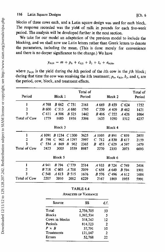
116 Latin Square Designs [Ch. 6
blocks of three cows each, and a Latin square design was used for each block.The response recorded was the yield of milk in pounds for each five-weekperiod. The analysis will be developed further in the next section.
We take for our model an adaptation of the previous model to include theblocking, and we shall now use Latin letters rather than Greek letters to denotethe parameters, including the mean. (This is done merely for convenienteand there is no deeper significance to the change.) We have
Yhtjk = M + ph + C{(p + bf + tk + ehiik,
where Yh{fk is the yield during the hth period of the ith cow in the jth block;during that time the cow was receiving the kth treatment; Ph , c{(j), b5, and tk arethe period, cow, block, and treatment effects.
Total of Total ofPeriod Block 1 Period Block 2 Period
1 A 768 B 662 C 731 2161 A 669 B 459 C 624 17522 B600 C 515 A 680 1795 C 550 A 409 B 462 14213 C411 A 506 B 525 1442 B 416 C 222 A 426 1064
Total of Cow 1779 1683 1936 5398 1635 1090 1512 4237
Block 3 Block 4
1 A 1091 B 1234 C 1300 3625 A 1105 B 891 C 859 28552 B 798 C 902 A 1297 2997 C 712 A 830 B 617 21593 C 534 A 869 B 962 2365 B 453 C 629 A 597 1679
Total of Cow 2423 3005 3559 8987 2270 2350 2073 6693
Block 5 Block 6
1 A 941 B 794 C 779 2514 A 933 B 724 C 749 24062 B 718 C 603 A 718 2039 C 658 A 649 B594 19013 C 548 A 613 B515 1676 B576 C 496 A 612 1684
Total of Cow 2207 2010 2012 6229 2167 1869 1955 5991
TABLE 6.4
ANALYSIS OF VARIANCE
Source SS d.f.
Total 2,756,705 53Blocks 1,392,534 5Cows in blocks 318,242 12Periods 814,223 2P x B 57,791 10Treatments 121,147 2Errors 52,768 22
Dow
nloa
ded
12/1
1/12
to 1
29.1
28.2
07.2
42. R
edis
trib
utio
n su
bjec
t to
SIA
M li
cens
e or
cop
yrig
ht; s
ee h
ttp://
ww
w.s
iam
.org
/jour
nals
/ojs
a.ph
p

Sec. 6.7] Change-Over Designs Balanced for Residual Effects 117
6.7 Change-Over Designs Balanced for Residual Effects
The change-over design that has just been discussed in the example is balancedfor treatments. It is also a balanced design for the comparison or elimination ofresidual effects, and it was as an illustration of this that Patterson (1950) pre-sented the data. When a cow that received treatment A for the first period isswitched to treatment B for the second period, the yield in the second period mayreflect not just the main effect of treatment B, but also the residual effect, if thereis one, of treatment A.
In the design, blocks I and II together form a pair of orthogonal Latin squares,
ABC ABC
BCA CAB
CA B B CA
and the same is true for blocks III and IV and for blocks V and VI. In the pair ofsquares, each treatment is used once on each of the six cows. There are noresidual effects during the first period. In the subsequent periods, the residualeffect of each treatment appears four times. In each of the last two periods, themain (or direct) effect of each treatment is observed in two cows, and theresidual effect of each treatment is also observed in two cows. Since no treat-ment can follow itself, no yield reflects both the main effect and the residualeffect of the same treatment. This problem was first considered by Cochran et al.(1941). Further developments are due to Patterson (1950) and (1952), and Lucas(1951) and (1957). The designs are also applicable to experiments, such as thoseinvolving the rotation of crops, in which several treatments are applied insuccession to the same experimental units.
In the general case with the dairy cattle, we make use of sp cows over p periods,and the feeding schedule is arranged in such a way that
(i) Each cow has each treatment for one period;(ii) In each period each treatment is used on s cows;
(iii) Each treatment follows every other treatment s times.
We shall not consider blocks in our analysis; they present only a minor complica-tion. The discussion given here is based on that of Patterson (1950).
A set of s of the cows receive the qth treatment in the last period, and there-fore never experience the residual effect of that treatment. We call the kth ofthat subset of s cows the (kq)th cow. Let Yhijkq denote the yield of the (kq)th cowduring the hth period in which she received the ith treatment, preceded, ifh > 1, by the jth treatment. Then
Yhilk4 = m + dh + ti + r1 + Ck9 + ehi5k9,
Dow
nloa
ded
12/1
1/12
to 1
29.1
28.2
07.2
42. R
edis
trib
utio
n su
bjec
t to
SIA
M li
cens
e or
cop
yrig
ht; s
ee h
ttp://
ww
w.s
iam
.org
/jour
nals
/ojs
a.ph
p
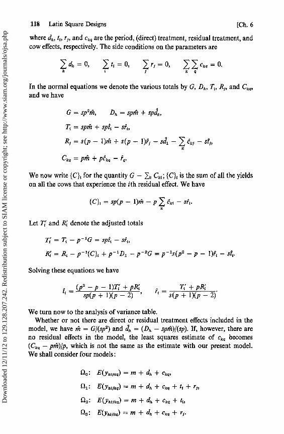
118 Latin Square Designs [Ch. 6
where dh , ti, ri, and Ckq are the period, (direct) treatment, residual treatment, andcow effects, respectively. The side conditions on the parameters are
1 di, =01 1 t1 = 0, r1=0, 11Ck9= 0 .h i j k q
In the normai equations we denote the various totals by G, Dh, Ti, R5, and Ckq,and we have
G = sp2ih, Dh = spin + spJh ,
Ti =spin +sp$i —sPi ,
R1 =s(p-1)»z+s(p-1)r"5 —sd1 —^ckf —si5 ,k
Ckq = p)h + PCkq — ry .
We now write {C}i for the quantity G — Ik Cki; {C} i is the sum of all the yieldson all the cows that experience the ith residual effect. We have
{C} i = sp(p — 1)m — p 5. cki — si.k
Let Ti and Ri denote the adjusted totals
Ti = Ti — p - 1 G = spti — sr"i,
Ri = Ri — p -1{C} i + p - 'D1 — p -2G = p -1s(p2 — p — 1)fi — s?i .
Solving these equations we have
_ (p2 — p — 1)T{ + pR{ Ti + pRiti sp(p + 1 )(P — 2) ' ri — s(P + 1 )(p — 2)
.
We turn now to the analysis of variance table.Whether or not there are direct or residual treatment effects included in the
model, we have m = G/(sp2) and cd,, = (Dh — spm)/(sp). If, however, there areno residual effects in the model, the least squares estimate of ckq becomes(Ckq — pm)/p, which is not the same as the estimate with our present model.We shall consider four models:
Oo: E(Yhtjk9) = m + dh + Ckq,
1: E(Yhiika) = m + dh + Ckq + ti + r5,
^2 : E (Yhilk9) = m + dh + Ckq + ti,
Ç : E(Yh15k4) = m + dh + Ckq + r!.
Dow
nloa
ded
12/1
1/12
to 1
29.1
28.2
07.2
42. R
edis
trib
utio
n su
bjec
t to
SIA
M li
cens
e or
cop
yrig
ht; s
ee h
ttp://
ww
w.s
iam
.org
/jour
nals
/ojs
a.ph
p
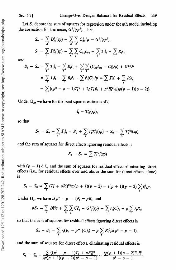
Sec. 6.7] Change-Over Designs Balanced for Residual Effects 119
Let S„ denote the sum of squares for regression under the nth model includingthe correction for the mean, G 2/(sp2). Then
So = Dhh/(sP) + Ga Ckq/P — G 2/(sp2),h k q
S1 = Dn/(sp) + Ckgekq + Tilt + Ri►'i,h k q t t
andSl — So = Tt it + Rtrt + (CkgCkq — Ckjjp) + G 2/N
t t k q
_ Ti lt + Rir"i — r"t{C}tlp = Ti fi + Rir"it t i t t
_ {(p2 — p — 1)T{ 2 + 2pTtRi + p 2Ri2}/{sp(p + 1)(p — 2)}.
Under SZ2 , we have for the least squares estimate of t i
ii = Til(sP),
so that
S2 = So + Ttft = So + T T, l (sp) = So + T{ 2/(sp),
and the sum of squares for direct effects ignoring residual effects is
S2 — So = : Ti 2/(sp)
with (p — 1) d.f., and the sum of squares for residual effects eliminating directeffects (i.e., for residual effects over and above the sum for direct effects alone)is
Sl — S2 = (Ti + PRí) 2/sp(P + 1 )(p — 2) = s(p + 1 )(P — 2) ri/p.t t
Under S23i we have s(p2 — p — 1)r1 = pR{, and
PS3 = Dh/s + Ckq — G 2/(sP) — r"i{C}t + p rtRt^h k q t i
so that the sum of squares for residual effects ignoring direct effects is
S3 — So = r"i(Rt — p -1{C} i) = p Ri2/s(p2 — p — 1),t t
and the sum of squares for direct effects, eliminating residual effects is
Si — S3 = 1i ((P2 — p — 1 )Ti + PRí) 2 —_ sp(P + 1 )(P — 2)y f2sp(P + 1 )(P — 2)(P2 — p — 1) p2 — p — 1
Dow
nloa
ded
12/1
1/12
to 1
29.1
28.2
07.2
42. R
edis
trib
utio
n su
bjec
t to
SIA
M li
cens
e or
cop
yrig
ht; s
ee h
ttp://
ww
w.s
iam
.org
/jour
nals
/ojs
a.ph
p
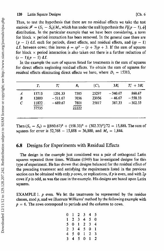
120 Latin Square Designs [Ch. 6
Thus, to test the hypothesis that there are no residual effects we take the teststatistic F = (S, — S2) /Me , which has under the null hypothesis the F[(p — 1), ¢]distribution. In the particular example that we have been considering, a termfor block x period interaction has been removed. In the general case there are(p — 1) d.f. each for periods, direct effects, and residual effects, and (sp — 1)d.f. between cows; this leaves ¢ = spe — (s + 3)p + 3. If the sum of squaresfor block x period interaction is allo taken out there is a further reduction of(s — 1)(p — 1) d.f.
In the example the sum of squares listed for treatments is the sum of squaresfor direct effects neglecting residual effects. To obtain the sum of squares forresidual effects eliminating direct effects we have, where D l = 15313,
T, Ti Rt {C}i 3Rí Tí + 3Ri
A 13713 1201.33 7385 25297 —340.67 860.67B 12000 —511.67 7036 23956 —46.67 —558.33C 11822 —689.67 7801 25817 387.33 —302.33
37535 22222
Then (S1 — S2) = [(860.67) 2 + (558.33)2 + (302.33) 2]/72 = 15,888. The sum ofsquares for error is 52,768 — 15,888 = 36,880, and Me = 1,844.
6.8 Designs for Experiments with Residual Effects
The design in the example just considered was a pair of orthogonal Latinsquares repeated three times. Williams (1949) has investigated designs for thistype of experiment. He has shown that designs balanced for the residual effect ofthe preceding treatment and satisfying the requirements listed in the previoussection can be obtained with only p cows, or replications, ifp is even, and with 2pcows ifp is odd, as was the case in the example. His designs are based upon Latinsquares.
EXAMPLE 1. p even. We let the treatments be represented by the residueclasses, mod p, and we illustrate Williams' method by the following example withp = 6. The rows correspond to periods and the columns to cows.
0 1 2 3 4 51 2 3 4 5 05 0 1 2 3 42 3 4 5 0 14 5 0 1 2 33 4 5 0 1 2
Dow
nloa
ded
12/1
1/12
to 1
29.1
28.2
07.2
42. R
edis
trib
utio
n su
bjec
t to
SIA
M li
cens
e or
cop
yrig
ht; s
ee h
ttp://
ww
w.s
iam
.org
/jour
nals
/ojs
a.ph
p
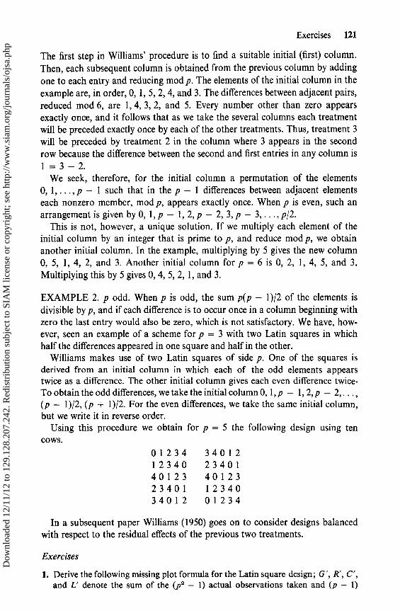
Exercises 121
The first step in Williams' procedure is to find a suitable initial (first) column.Then, each subsequent column is obtained from the previous column by addingone to each entry and reducing mod p. The elements of the initial column in theexample are, in order, 0, 1, 5, 2, 4, and 3. The differences between adjacent pairs,reduced mod 6, are 1, 4, 3, 2, and 5. Every number other than zero appearsexactly once, and it follows that as we take the several columns each treatmentwill be preceded exactly once by each of the other treatments. Thus, treatment 3will be preceded by treatment 2 in the column where 3 appears in the secondrow because the differente between the second and first entries in any column is1 = 3 - 2.
We leek, therefore, for the initial column a permutation of the elements0, 1, .. ., p - 1 such that in the p - 1 differences between adjacent elementseach nonzero member, mod p, appears exactly once. When p is even, such anarrangement is given by 0, 1, p - 1, 2, p - 2, 3, p - 3.....p/2.
This is not, however, a unique solution. If we multiply each element of theinitial column by an integer that is prime to p, and reduce mod p, we obtainanother initial column. In the example, multiplying by 5 gives the new column0, 5, 1, 4, 2, and 3. Another initial column for p = 6 is 0, 2, 1, 4, 5, and 3.Multiplying this by 5 gives 0, 4, 5, 2, 1, and 3.
EXAMPLE 2. p odd. When p is odd, the sum p(p - 1)/2 of the elements isdivisible by p, and if each difference is to occur once in a column beginning withzero the last entry would also be zero, which is not satisfactory. We have, how-ever, seen an example of a scheme for p = 3 with two Latin squares in whichhalf the differences appeared in one square and half in the other.
Williams makes use of two Latin squares of side p. One of the squares isderived from an initial column in which each of the odd elements appearstwice as a differente. The other initial column gives each even difference twice.To obtain the odd differences, we take the initial column 0, 1, p - 1, 2, p - 2, ... ,(p - 1)/2, (p + 1)/2. For the even differences, we take the same initial column,but we write it in reverse order.
Using this procedure we obtain for p = 5 the following design using tencows.
01234 3401212340 2340140123 4012323401 1234034012 01234
In a subsequent paper Williams (1950) goes on to consider designs balancedwith respect to the residual effects of the previous two treatments.
Exercises
1. Derive the following missing plot formula for the Latin square design; G', R', C',and L' denote the sum of the (p 2 - 1) actual observations taken and (p - 1)
Dow
nloa
ded
12/1
1/12
to 1
29.1
28.2
07.2
42. R
edis
trib
utio
n su
bjec
t to
SIA
M li
cens
e or
cop
yrig
ht; s
ee h
ttp://
ww
w.s
iam
.org
/jour
nals
/ojs
a.ph
p

122 Latin Square Designs [Ch. 6
actual observations occurring in the same row, column, and with the same letter asthe missing plot.
x= p(R' + C' + L') —2G '
(p — 1 )(P — 2)
Show that if the missing plot received the ith treatment and is replaced by a valuecalculated by the previous formula then
V(Th —T )=Qa \P + (P — 1)(p - 2)/
2. Youden and Hunter (1955) suggested modifying the Latin square design in thefollowing way to obtain an unbiased estimate of the error. They chose a squarein which each variety appeared exactly once on the diagonal and duplicated thoseplots, thus obtaining an estimate of error between duplicates with p degrees offreedom. Because the design is no longer orthogonal the analysis calls for testingsubhypotheses: rows, columns (after rows), and treatments (after columns androws). Derive the analysis.
3. Suppose that one entire row is omitted from a Latin square design and modify theanalysis accordingly.
4. For the data for the dairy cattle experiment, compute
(i) the sum of squares for residual effects ignoring direct effects, and(ii) the sum of squares for direct effects eliminating the residual effects.
Dow
nloa
ded
12/1
1/12
to 1
29.1
28.2
07.2
42. R
edis
trib
utio
n su
bjec
t to
SIA
M li
cens
e or
cop
yrig
ht; s
ee h
ttp://
ww
w.s
iam
.org
/jour
nals
/ojs
a.ph
p

CHAPTER 7
Factors withTwo or
Three Levels;Confounding
In the previous chapters we have developed the analysis of variance for thegeneral multifactorial experiment. We finished up with algorithms for obtainingdegrees of freedom, sums of squares, and expected mean squares for fixed,mixed, or random models. The only blocking situation considered was that ofthe randomized complete block, in which case the blocks appeared in thealgorithms as the levels of another (random) factor.
In this chapter we shall take another look at the factorial experiment. The2n and 3' factorials will be introduced. We shall also consider blocking in thecase in which the blocks are not large enough to contain all the treatments, asituation which we saw for the first time in the split-plot design where each wholeplot contained only one level of each of the main treatments. We shall assumethroughout that all the factors have fixed effects, that the block effects arerandom effects with mean zero and variance aB, uncorrelated with each otheror with the error terms, and that there is no interaction between blocks andtreatments. We mean by the last statement that if y jƒ denotes an observation onthe ith treatment in the jth block, and y denotes an observation on the hthtreatment in the same block, then, apart from random error, the differenceYhj — yij remains the same for all values of j.
The reader will not fail to notice the enormous contribution made by Yatesto the development of the topics covered in this chapter. In particular, numerousreferences will be found to his pioneer monograph, The Design and Analysis ofFactorial Experiments, which was published in 1937 as Technical Communication35 by the Imperial Bureau of Soil Science, Harpenden, England.
123
Dow
nloa
ded
12/1
1/12
to 1
29.1
28.2
07.2
42. R
edis
trib
utio
n su
bjec
t to
SIA
M li
cens
e or
cop
yrig
ht; s
ee h
ttp://
ww
w.s
iam
.org
/jour
nals
/ojs
a.ph
p
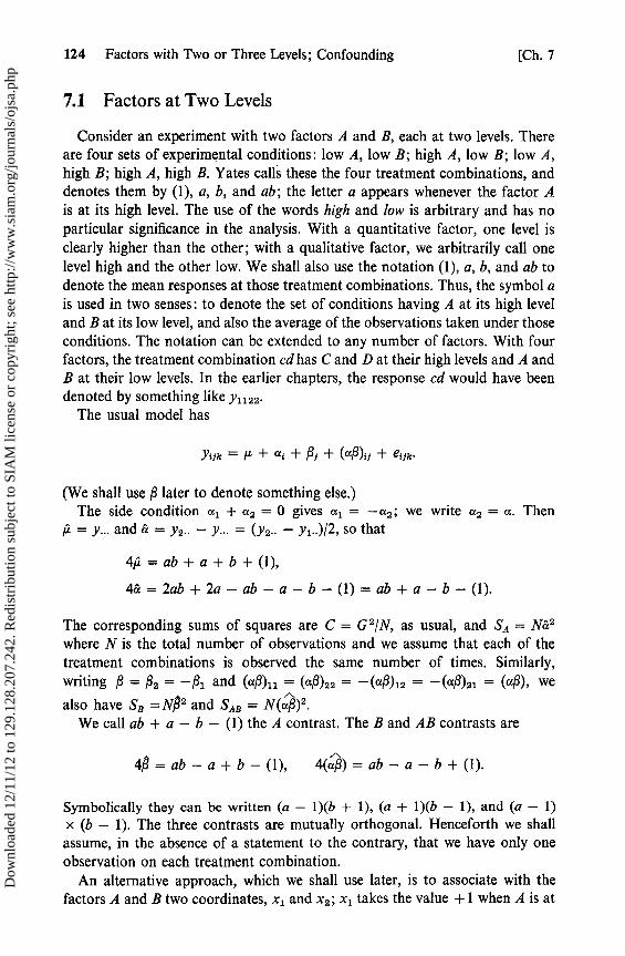
124 Factors with Two or Three Levels; Confounding [Ch. 7
7.1 Factors at Two Levels
Consider an experiment with two factors A and B, each at two levels. Thereare four sets of experimental conditions: 1ow A, low B; high A, low B; low A,high B; high A, high B. Yates calls these the four treatment combinations, anddenotes them by (1), a, b, and ab; the letter a appears whenever the factor Ais at its high level. The use of the words high and low is arbitrary and has noparticular significance in the analysis. With a quantitative factor, one level isclearly higher than the other; with a qualitative factor, we arbitrarily call onelevel high and the other low. We shall also use the notation (1), a, b, and ab todenote the mean responses at those treatment combinations. Thus, the symbol ais used in two senses: to denote the set of conditions having A at its high leveland B at its low level, and also the average of the observations taken under thoseconditions. The notation can be extended to any number of factors. With fourfactors, the treatment combination cd has C and D at their high levels and A andB at their low levels. In the earlier chapters, the response cd would have beendenoted by something like Y1122.
The usual model has
Ysik = N- + at + Pi + (aP)ti + etirc.
(We shall use P later to denote something else.)The side condition al + a2 = 0 gives al = —a2i we write a2 = a. Then
µ = y... and & = Y2.. — Y... =(Y2.. — yl..)/2, so that
4µ= ab+a+b+(1),
4á= 2ab+2a—ab—a—b—(1)=ab+a—b—(1).
The corresponding sums of squares are C = G 2/N, as usual, and SA = N&2
where N is the total number of observations and we assume that each of thetreatment combinations is observed the same number of times. Similarly,writing N = NZ = — P1 and (aN)11 = (a)22 = — (aP)12 = — (aa)21 = (aN), we
also have SB =NO2 and SAB = N( P)2 .
We call ab + a — b — (1) the A contrast. The B and AB contrasts are
4ft= ab—a+b—(1), 4(è)= ab—a—b+(1).
Symbolically they can be written (a — 1)(b + 1), (a + 1)(b — 1), and (a — 1)x (b — 1). The three contrasts are mutually orthogonal. Henceforth we shallassume, in the absence of a statement to the contrary, that we have only oneobservation on each treatment combination.
An alternative approach, which we shall use later, is to associate with thefactors A and B two coordinates, xl and x2 ; xl takes the value + 1 when A is at
Dow
nloa
ded
12/1
1/12
to 1
29.1
28.2
07.2
42. R
edis
trib
utio
n su
bjec
t to
SIA
M li
cens
e or
cop
yrig
ht; s
ee h
ttp://
ww
w.s
iam
.org
/jour
nals
/ojs
a.ph
p
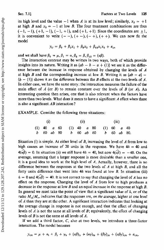
Sec. 7.1 ] Factors at Two Levels 125
its high level and the value —1 when A is at its low level; similarly, x2 = + 1at high B and x2 = — 1 at low B. The four treatment combinations are thus(-1, —1), (+ 1, —1), (-1, + 1), and (+ 1, + 1). Since the coordinates are ± 1,it is convenient to write (— —), (+ —), (— +), (+ +). We can now fit themodel
YiJ = Po + flixi + P2x2 + R12x1x2 + e1,
and we shall have Po = µ, P1 = a, P2 = P, P12 = (aP).The interaction contrast may be written in two ways, both of which provide
insights into its nature. Writing it as {ab — b — a + ( l)} we see it as the differ-ence between the increase in response obtained by changing the levels of Aat high B and the corresponding increase at low B. Writing it as {ab — a} —{b — ( 1)} shows it as the difference between the B effects at the two levels of A.In either case, we have the same story: the interaction measures the failure of themain effect of A (or B) to remain constant over the levels of B (or A). Aninteresting question then arises, one that is also relevant when the factors havemore than two levels. What does it mean to have a significant A effect when thereis also a significant AB interaction?
EXAMPLE. Consider the following three situations:
(i)
(ii)
(iii)
(1) 40 a 60
(1) 40 a 80 (1) 60 a 40b 60 ab 80
b 60 ab 60 b 60 ab 80.
Situation (i) is simple. At either level of B, increasing the level of A from low tohigh causes an increase of 20 units in the response. We have 4« = 40 and
4(a) = 0. In situation (ii) we stilt have 4& = 40, but now 4(aa) _ — 40. On theaverage, assuming that a larger response is more desirable than a smaller one,it is a good idea to work at the high level of A. Actually, however, there is nodifference between the responses at the two levels of A at high B, and all theforty units difference- that went into 4& was found at low B. In situation (iii)
« = 0 and 4(«a) = 40. It is not correct to say that changing the level of A has noeffect on the response. Changing the level of A from low to high produces adecrease in the response at low B and an equal increase in the response at high B.In general we must take the point of view that a significant value of «, or of theratio M4/Me , indicates that the responses are, on the average, higher at one levelof A than they are at the other. A significant interaction indicates that looking atthe average change in response is not enough, and that the effect of changinglevels of A is not the same at all levels of B; equivalently, the effect of changinglevels of B is not the same at all levels of A.
If we add a third factor, C, also at two levels, we introduce a three-factorinteraction. The model becomes
Ytik = N + ai + fl + Yk + ( X)ij + (aM)uo + (fY),k + (afY)iik + efjk,
Dow
nloa
ded
12/1
1/12
to 1
29.1
28.2
07.2
42. R
edis
trib
utio
n su
bjec
t to
SIA
M li
cens
e or
cop
yrig
ht; s
ee h
ttp://
ww
w.s
iam
.org
/jour
nals
/ojs
a.ph
p

126 Factors with Two or Three Levels; Confounding [Ch. 7
and, proceeding as before, we have
811=abc+ab+ac+bc+a+b+c+(1),
8&=abc+ab+ac—bc+a—b—c—(1),
8(a) = abc + ab — ac — bc — a — b + c + (1),
which may be written symbolically as (a + 1)(b + 1)(c + 1), (a — 1)(b + 1)x (c + l), and (a — 1)(b — 1)(c + 1).
The eight interaction terms (a!y), ik have the same absolute value. If they arenot all zero, four of them are positive and the other four are negative. The sideconditions
11(ajY)í>k = 0, 11(aPY)tik = 0, ^1, (aSY)tlk = 04 j 4 k ! k
lead to
(aNY)22a = — ("PY)221 = — (aaY)212 = — (afY)122 = (aaY)211 = (aPY)1a1
= (aaY)112 = — (afY)111 = (afY),
whence
8(afly)=abc—bc—ac—ab+a+b+c—(1).
Alternatively, we may write the model as
E(y) = Ro + Rlxl + 192x2 + 93x3 + P12x1x2
+ P13x1x3 + P23x2x3 + N123x1x2x3•
Then 8P123 = (responses at those points with x1x2x3 = 1) — Y (responses at
those points with x1x2x3 = —1) = 8(apy). Symbolically we have 8(aay) _
8$123 = (a — 1)(b — 1)(c — 1).There are several notations that can be used to denote the ABC contrasts and,
similarly, other contrasts. We shall use either {ABC} or {x1x2x3}. We shall alsouse {x1x2x3 = + 1} and {xlx2x3 = —1} to denote the sums of the responses atthe points at which x 1x2x3 = +1 or —1, respectively. Then {ABC} = {x1x2x3} _{x1x2x3 = + 1} — {x 1x2x3 = — 1}. Yates has denoted ABC by A.B.C..
The ABC contrast can be written (abc — ac — bc + c) — (ab — a — b + (1)),which is the difference between the AB contrast at high C and the AB contrastat low C. It may also be considered as the difference between the AC contrasts atthe two levels of B, or the difference between the BC contrasts at the two levelsof A.
Dow
nloa
ded
12/1
1/12
to 1
29.1
28.2
07.2
42. R
edis
trib
utio
n su
bjec
t to
SIA
M li
cens
e or
cop
yrig
ht; s
ee h
ttp://
ww
w.s
iam
.org
/jour
nals
/ojs
a.ph
p

Sec. 7.2] Yates' Algorithm and the General 2n Design 127
The variance of the estimate of any effect, either main effect or interaction, isN -102 . Each point contributes with the same weight to the estimate of eacheffect. In particular, so far as the estimation of a is concerned, we have lostnothing in precision by adding B and C to the experiment because the varianceof P1 in this experiment is the same as it would have been if we had not had thefactors B and C and had made instead only four runs at low A and four runs athigh A. Alternatively, we may take the point of view that the addition of theextra factor C to the experiment also adds two more points at high A and at lowA, and two more at high B and low B for estimating A, B, and AB. This is anexample of what is sometimes referred to as the hidden replication property ofthe factorial experiment.
We have in the 23 experiment four direct comparisons to estimate the maineffect of A, namely, a — (1), ab — b, ac — c, and abc — bc. We obtain a vividpictorial representation when the experimental points are portrayed as thevertices of a cube with coordinates (± 1, ± 1, ± 1).
bc 24 abc 40
c 20
30
(1) 12 a 22
The four constituent A contrasts are 10, 12, 10, and 16. The overall A contrastis the sum, 48, with an average of 12. At low B we have A contrasts 10 and 10;at high B we have 12 and 16, giving an interaction contrast 28 — 20 = 8. At lowC the AB contrast is 12 — 10 = 2; at high C the AB contrast is 16 — 10 = 6;the ABC contrast is 6 — 2 = 4.
7.2 Yates' Algorithm and the General 2n Design
The 2' design is the complete factorial for n factors, each at two levels. Wehave now seen enough to be able to tell how the derivation of the contrasts willproceed. If 0 is some effect (and we emphasize that we use the term effect toembrace both main effects and interactions), the contrast will be the symbolicproduct given by
{O} = 2n0 _ (a ± 1)(b ± 1)(c ± 1) ...,
Dow
nloa
ded
12/1
1/12
to 1
29.1
28.2
07.2
42. R
edis
trib
utio
n su
bjec
t to
SIA
M li
cens
e or
cop
yrig
ht; s
ee h
ttp://
ww
w.s
iam
.org
/jour
nals
/ojs
a.ph
p

128 Factors with Two or Three Levels; Confounding [Ch. 7
where the sign of ± 1 is negative for all those letters appearing in 0 and positiveelsewhere. Thus, in a 2 6 experiment we should have
64135 = 64(ACE) = (a — 1)(b + 1)(c — 1)(d + 1)(e — 1)(f + 1).
We shall, henceforth, use upper case letters such as ACE to denote either theeffects or their estimates in a particular experiment. We shall no longer write thehat over ACE unless its omission would cause confusion. Some statisticiansprefer to take as the effects twice the corresponding regression coefficients, e.g.,A = 2 1 rather than A = as we do. Their procedure corresponds to a changefrom xl = —1 to x l = +1 rather than a change from x l = 0 to xl = + 1.
Based on the symbolic product rule, Yates developed an algorithm forcomputing the contrasts in a 2n design. We now illustrate the algorithm with thedata for the 2 design. There are several steps.
(i) The data are listed in the standard order (1), a; then b, ab; then c, ac, bc,abc, and so on; they are entered in this order in column 1.
(ii) The first 2n -1 entries in any of the subsequent columns are obtained byaddition. The entry in the ith row of the (k + l)th column is the sum ofthe (2i — 1)th and the (2i)th entries in the kth column.
(iii) The next 2'' entries are differences. The (2'' + i)th entry in the(k + 1)th column is obtained from the kth column by subtracting the(2i — l)th entry from the (2i)th entry. It is easy to make a mistake inthe sign at this stage.
(iv) The entries in the (n + 1)th column are the grand total M, followed bythe contrasts in standard order.
(v) W, X, Y, and Z are part of the checking procedure. W is the sum of theentries in rows 1, 3, ... , 2n -1 — 1, and X is the sum of the entries in rows2, 4, ... , 2" -1 . Y and Z are the corresponding sums for the second half ofthe table. The check in the calculations is that in any column X + W isequal to X + W + Z + Yin the previous column, and Z + Yis equal toX — W + Z — Y in the previous column.
(vi) We may add an extra column, the (n + 2)th, for the sum of the squares ofthe contrasts. The entries in this column are obtained by squaring theentries in the (n + 1)th column and dividing by 2. The sum of theentries in this column is equal to the sum of the squares of the originalobservations.
The calculations in this algorithm are notoriously error prone, especially inrespect to wrong signs used in recording the differences. Three other methods ofchecking the calculations are given in the literature. Good (1960), in an addendumto his earlier paper (1958) on the topic, suggests reversing the order of theelements of the (n + 1)th column so as to begin with ABC and end with M.The Yates procedure is now carried out on these figures, and the new (n + 1)thcolumn will have for its entries the original data, multiplied by 2n, in the reverse
Dow
nloa
ded
12/1
1/12
to 1
29.1
28.2
07.2
42. R
edis
trib
utio
n su
bjec
t to
SIA
M li
cens
e or
cop
yrig
ht; s
ee h
ttp://
ww
w.s
iam
.org
/jour
nals
/ojs
a.ph
p
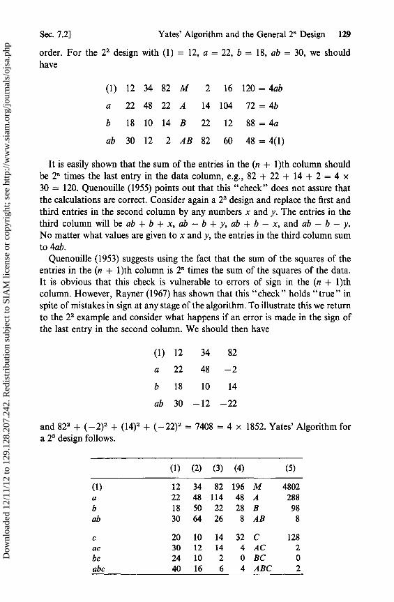
Sec. 7.2] Yates' Algorithm and the General 2" Design 129
order. For the 22 design with (1) = 12, a = 22, b = 18, ab = 30, we shouldhave
(1) 12 34 82 M 2 16 120 = 4ab
a 22 48 22 A 14 104 72 = 4b
b 18 10 14 B 22 12 88 = 4a
ab 30 12 2 AB 82 60 48 = 4(1)
It is easily shown that the sum of the entries in the (n + l)th column shouldbe 2' times the last entry in the data column, e.g., 82 + 22 + 14 + 2 = 4 x30 = 120. Quenouille (1955) points out that this "check" does not assure thatthe calculations are correct. Consider again a 22 design and replace the first andthird entries in the second column by any numbers x and y. The entries in thethird column will be ab + b + x, ab — b + y, ab + b — x, and ab — b — y.No matter what values are given to x and y, the entries in the third column sumto 4ab.
Quenouille (1953) suggests using the fact that the sum of the squares of theentries in the (n + 1)th column is 2' times the sum of the squares of the data.It is obvious that this check is vulnerable to errors of sign in the (n + 1)thcolumn. However, Rayner (1967) has shown that this "check" holds "true" inspite of mistakes in sign at any stage of the algorithm. To illustrate this we returnto the 22 example and consider what happens if an error is made in the sign ofthe last entry in the second column. We should then have
(1) 12 34 82
a 22 48 —2
b 18 10 14
ab 30 —12 —22
and 822 + (_2)2 + (14)2 + (*22)2 = 7408 = 4 x 1852. Yates' Algorithm fora 23 design follows.
(1) (2) (3) (4) (5)
(1) 12 34 82 196 M 4802a 22 48 114 48 A 288b 18 50 22 28 B 98ab 30 64 26 8 AB 8
c 20 10 14 32 C 128ac 30 12 14 4 AC 2bc 24 10 2 0 BC 0abc 40 16 6 4 ABC 2
Dow
nloa
ded
12/1
1/12
to 1
29.1
28.2
07.2
42. R
edis
trib
utio
n su
bjec
t to
SIA
M li
cens
e or
cop
yrig
ht; s
ee h
ttp://
ww
w.s
iam
.org
/jour
nals
/ojs
a.ph
p

130 Factors with Two or Three Levels; Confounding [Ch. 7
(1) (2) (3) (4)
W 30 84 104X 52 112 140Y 44 20 16Z 70 28 20X + W 82 196 244 280X — W 22 28 36Z + Y 114 48 36 40Z— Y 26 8 4X + W+Z+ Y 196 244 280X— W+Z— Y 48 36 40
7.3 The 3n Series of Factorials
The 3n factorial experiment has n factors, each at three levels. An example of. a3 3 experiment appeared in Chapter 5. We denote the levels of the factors by0, 1, and 2. Then the treatment combination with A and C at level 1 and B atlevel 2 may be denoted by 121 or a1b2c1 or ab2c. We shall use either of the firsttwo notations as convenient, and we shall sometimes not mention factors at theirlow levels, writing b1 c2 for the point with A at level 0, B at level 1, and C atlevel 2.
To illustrate the 3 2 experiment we take some of the data from the 3 3 experimentof Chapter 5. Subtracting 80 and rounding off we obtain
(1) 9, al 15, a2 20,
bl 7, albe 5, a2b 1 13,
b2 6, albe 1, a2b2 15.
TABLE 7.1ANALYSIS OF VARIANCE
Total 8 d.f. 1211 — 920.1 = 290.9
SA 2 1076.3 — 920.1 = 156.2lin A 1 112.7quad A 1 43.5SE 2 1015 — 920.1 = 94.9lin B 1 80.7quad B 1 14.2SAS 4 39.8
The interaction sum of squares is usually subdivided in one of two ways. Thefirst method involves the use of orthogonal Latin squares. As was pointed out in
Dow
nloa
ded
12/1
1/12
to 1
29.1
28.2
07.2
42. R
edis
trib
utio
n su
bjec
t to
SIA
M li
cens
e or
cop
yrig
ht; s
ee h
ttp://
ww
w.s
iam
.org
/jour
nals
/ojs
a.ph
p

Sec. 7.3] The 3" Series of Factorials 131
Chapter 6, a (p x p) Latin square is a square array of side p in which p lettersare arranged in such a way that each letter appears exactly once in each row andeach column. Two particular Latin squares of side 3 are
FQR P' Q R
QRF and RFQ
RPQ Q R P.
These two squares have an additional property. If the second square is super-imposed on the first square, each letter in the first square will appear exactlyonce with each letter in the second square. Such a pair of squares is said to beorthogonal. If we denote the coordinates (levels) for A and B by xl and x2 ,respectively, P occupies in the first square those places for which x l + x2 - 0(mod 3), while for Q we have xl + x2 = 1 (mod 3), and for R, xl + x2 = 2(mod 3). The totals for the letters are P 23, Q 37, R 31. Any contrast betweenthe letter totals is orthogonal to any contrast in the A totals or in the B totals.We can, therefore, calculate a sum of squares between the letters in square 1with 2 d.f. as (23 2 + 372 + 3 1 2)/3 — 920.1 = 32.9. Alternatively, we could taketwo orthogonal contrasts in the totals such as P — Q and P + Q — 2R and addtheir individual sums of squares to obtain (-14) 2/6 + (-2)2/18 = 32.9. Forthe second square, the letter totals are P 29, Q 34, R 28. Any contrast in thesetotals is orthogonal to any of the previous contrasts, and we have another sumof squares, also with 2 d.f.: (29 2 + 342 + 282)/3 — 920.1 = 6.9. The sum ofthe two components is 32.9 + 6.9 = 39.8 = SAB. Because their derivationsinvolve the sets of points defined by xl + x2 - 0, 1, 2 (mod 3) and byxl + 2x2 = 0, 1, 2 (mod 3), respectively, they are sometimes called the sums ofsquares for AB and AB2 interactions respectively.
For the 33 design we may subdivide SAB , SAc, and SBC in the same way.SABc with 8 d.f. can be divided into four constituent sums of squares, each with 2d.f., by breaking up the twenty-seven points into three sets of nine points each infour orthogonal ways. We then have
ABC: xl + x2 + x3 - 0, 1, 2 (mod 3),
AB2C: xl + 2x2 + x3 =_ 0, 1, 2 (mod 3),
ABC2 : xl + x2 + 2x3 = 0, 1, 2 (mod 3),
AB2C2: xl + 2x2 + 2x3 = 0, 1, 2 (mod 3).
Yates calls the sums of squares for AB and AB2 in the 3 2 design the sums ofsquares for the J diagonals and the I diagonals, respectively. He calls theclassifications that we have used for the 3 3 design Z, X, Y, and W, respectively.
The second approach is to split up the sum SAB into single degrees of freedomfor lin A lin B, and so on. We should then have the following four componentsums of squares: lin A lin B 1.0; lin A quad B 5.3; quad A lin B 33.3; quad A
Dow
nloa
ded
12/1
1/12
to 1
29.1
28.2
07.2
42. R
edis
trib
utio
n su
bjec
t to
SIA
M li
cens
e or
cop
yrig
ht; s
ee h
ttp://
ww
w.s
iam
.org
/jour
nals
/ojs
a.ph
p
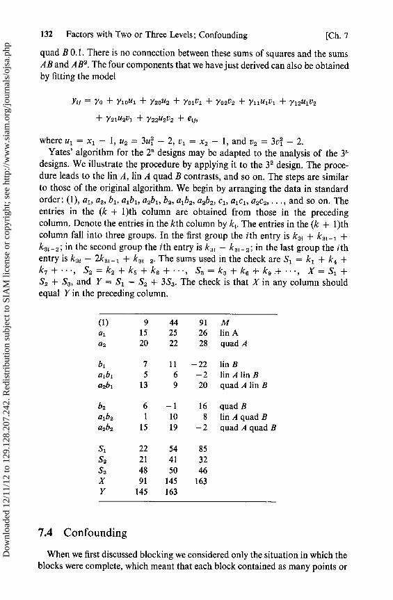
132 Factors with Two or Three Levels; Confounding [Ch. 7
quad B 0.1. There is no connection between these sums of squares and the sumsAB and AB2 . The four components that we have just derived can also be obtainedby fitting the model
Yti = Yo + Yioui + Y2ou2 + Yoivi + Y02v2 + Y11u1 v1 + Y12U1 V 2
+ Y21U2V1 + Y22U2V2 + ejj,
where ul = xi — 1, u2 = 3u1 — 2, v l = x2 — 1, and v2 = 3v1 — 2.Yates' algorithm for the 2n designs may be adapted to the analysis of the 3Ty
designs. We illustrate the procedure by applying it to the 3 2 design. The proce-dure leads to the lin A, lin A quad B contrasts, and so on. The steps are similarto those of the original algorithm. We begin by arranging the data in standardorder: (1), a,, a2, b1, albl, a2b1, b2, a1b2, a2b2, cl, alcl, a2c2, ..., and so on. Theentries in the (k + 1)th column are obtained from those in the precedingcolumn. Denote the entries in the kth column by ki . The entries in the (k + 1)thcolumn fall into three groups. In the first group the ith entry is k3i + k31 1 +k3i_2; in the second group the ith entry is k, — k_2; in the last group the ithentry is k31 — 2k3i _ 1 + k31 _ 2 . The sums used in the check are S l = kl + k4 +k7 +•••, S2= k2 +k5 +k8 +•••, S3=k3 +k6 +k9 +•• , X=S1 +S2 + S3 , and Y = Sl — S2 + 3S3 . The check is that X in any column shouldequal Y in the preceding column.
(1) 9 44 91 Mal 15 25 26 lin Aa2 20 22 28 quad A
bl 7 11 —22 lin Balbe 5 6 —2 lin A lin Ba2b1 13 9 20 quad A lin B
b2 6 —1 16 quad Bajb2 1 10 8 lin A quad Ba2b2 15 19 —2 quad A quad B
S1 22 54 85S2 21 41 32S3 48 50 46X 91 145 163Y 145 163
7.4 Confounding
When we first discussed blocking we considered only the situation in which theblocks were complete, which meant that each block contained as many points or
Dow
nloa
ded
12/1
1/12
to 1
29.1
28.2
07.2
42. R
edis
trib
utio
n su
bjec
t to
SIA
M li
cens
e or
cop
yrig
ht; s
ee h
ttp://
ww
w.s
iam
.org
/jour
nals
/ojs
a.ph
p
Sec. 7.4] Confounding 133
plots as there were treatments or treatment combinations. We turn our attentionnow to the situation which arises in a factorial experiment when the block size istoo small to accomodate one plot with each of the treatment combinations, butis large enough for some fraction of them. We begin by discussing a 2 2 experi-ment in two blocks of two points each. We shall refer to the experimental pointsas points or runs; the Jatter is a common usage among chemical engineers whospeak of making a run on their pilot plant at some set of conditions.
We have three choices for the division into blocks:
(i) (1), a; b, ab;(ii) (1), b; a, ab;(iii) (1), ab; a, b.
The revised model, including the block effects, may be written
Yijg = PO + N1x1 + P2X2 + P12X1X2 + sg + eij,
where Yijg is the response at the ith level of A and the jth level of B in the gthblock, and 8g is the gth block effect, which we now treat as fixed. The usual sidecondition lg Sg = 0 becomes 8 + 62 = 0, and so we write 8 1 = — 6 andS2=+ 8.
Consider blocking scheme (i). The experimental points in block I are both atlow B. The experimental points in block II are both at high B. Hence, theexpectation of the B contrast is (using the suffix 1 to denote the low level of afactor and 2 for the high level)
E{B} = E(y22 + Y12 — Y21 — Y11) = 4P2 + 48.
On the other hand, E{A} = 4P 1 and E{AB} = 4P 12 .
Another way of looking at the situation is to say that, since both points in oneblock are at high B and both points in the other block are at low B, we cannot,when we look at the B contrast, tell whether the observed difference results fromthe B effect, from block differences, or from a combination of both. On theother hand, each block contains one treatment combination at high A and one atlow A, and so the block effects 8 cancel out; they also cancel out for the ABcontrast. We say, therefore, that the B effect is completely confounded, i.e.,confused, with blocks. In scheme (ii), A is confounded but B and AB are not.In practice most experimenters would choose scheme (iii) because here it is thetwo-factor interaction AB that is confounded, while the main effects A and Bare clear of the block effects.
When we consider dividing the 2 design into two blocks of four runs each,there are more options; indeed, there are thirty-five possible ways in which tochoose three treatment combinations out of leven to be put in the same block as(1). One possibility is to take as the first block (1), a, b, c, which is the traditionalone-at-a-time experiment (inasmuch as we start at the base point and vary
Dow
nloa
ded
12/1
1/12
to 1
29.1
28.2
07.2
42. R
edis
trib
utio
n su
bjec
t to
SIA
M li
cens
e or
cop
yrig
ht; s
ee h
ttp://
ww
w.s
iam
.org
/jour
nals
/ojs
a.ph
p
134 Factors with Two or Three Levels; Confounding [Ch. 7
A, B, and C singly in turn). With this blocking the expected value of the contrastbetween block totals is
E{abc + ab + ac + bc — a — b — c — (1)}
= 88 + 441+ 4P2 + 453 - 4123.
The expectation of the A contrast is 8P1 + 48. All three main effects and thethree-factor interaction are confounded with blocks.
We can, however, arrange the blocking so that one and only one of theeffects is confounded. This we achieve by taking any one of the leven contrastsfor estimating effects, and placing in one block all the treatment combinationsthat appear with a positive sign in the contrast and in the other block thosetreatment combinations that have a negative sign. The chosen contrast will thenbe identical with the difference between block totals, and the chosen effect will becompletely confounded with block effects. However, the estimating contrasts aremutually orthogonal, and so the other contrasts are orthogonal to the contrast inthe block totals; the other effects are clear of the block biases.
If we decided to confound ABC with blocks, the division would be
block I abc, a, b, c; block II ab, ac, bc, (1).
We note that in each block there are exactly two points at the high level of Aand two at the low level; the same is true for B and C. Block I consists of all thetreatment combinations with positive signs in the ABC contrast; we shall callthem the set of points defined by I = +ABC. They are also the set of points forwhich x 1x2x3 = + 1. The other block contains the set of points defined byI = —ABC or by x 1x2x3 = — 1. In general, let P be any effect. We shall call theset of points that have positive (or negative) signs in the P contrast the set (orfraction of the 2n points) defined by 1 = +P (or by I = —P).
The chosen contrast is said to be the defining contrast of the confoundingscheme. The analysis proceeds as before, using Yates' algorithm, except that thesum of squares for the defining contrast is discarded, since it is biased by theblock effects. The extension to blocking the general 2n design into two blocks of2n -1 points each is obvious. When there are more than two blocks the situationis more interesting; this will be discussed later.
7.5 Partial Confounding
1f the experiment contains several replications, i.e., if the set of treatmentcombinations is to be repeated several times instead of only once, we have twochoices. Either we can repeat the same basic design each time, which wouldamount in our example to dividing each replicate into two blocks alwaysconfounding ABC, or else we can confound one or more of the other effects inthe subsequent replications. Thus, if the experiment were to call for four
Dow
nloa
ded
12/1
1/12
to 1
29.1
28.2
07.2
42. R
edis
trib
utio
n su
bjec
t to
SIA
M li
cens
e or
cop
yrig
ht; s
ee h
ttp://
ww
w.s
iam
.org
/jour
nals
/ojs
a.ph
p
Sec. 7.5] Partial Confounding 135
replicates we might elect to confound ABC in the first replicate, AB in the secondreplicate, AC in the third, and BC in the fourth. In that case the four interactionsare said to be partially confounded with blocks. Each of them is completelyconfounded with blocks in one of the replicates, but it is unconfounded in theother three replicates. We thus lose 25 per cent of the information about each ofthe interactions by dividing the thirty-two observations into eight blocks of fourpoints each.
The experimenter has, therefore, two choices. He can either elect to learnnothing about the three-factor interaction while at the same time retaining 100per cent information about each of the two-factor interactions, or he can obtainestimates of all four interactions at the colt of an increase in variance for theestimates of AB, AC, and BC. This is a choice which he himself must make indesigning his experiment.
AN EXAMPLE OF PARTIAL CONFOUNDING. The following example,given by Yates (1937), deals with an experiment on potatoes. The factors areA, sulphate of ammonia; B, sulphate of potash; and C, nitrogen (manure). Theresponses are the yields in pounds per plot.
(1) 101 c 312 (1) 106 b 272ac 373 a 106 ab 306 a 89bc 398 b 265 c 324 bc 407ab 291 abc 450 abc 449 ac 338
1163 1133 1185 1106la Ib IIa IIb
(1) 87 c 323 (1) 131 c 324ac 324 a 128 a 103 ac 361b 279 bc 423 bc 445 b 302abc 471 ab 334 abc 437 ab 272
1161 1208 1116 1259IIIa IIIb IVa IVb
Using Yates' algorithm for each of the four replicates separately, we obtain thefollowing totals and contrasts. The entries in the last column are the row totals.The underlined contrasts are those that are confounded with blocks, and theyare not included in the corresponding row totals.
The estimates of the unconfounded effects are obtained by dividing thecorresponding totals by 32; for the partially confounded interactions thedivisor is 24. In Table 7.2 the rums of squares for the effects are obtained bysquaring the row totals and dividing by 32 or 24, as appropriate, the divisorbeing the number of observations that went into the total.
The results of applying Yates' algorithm to the replicates follow.
Dow
nloa
ded
12/1
1/12
to 1
29.1
28.2
07.2
42. R
edis
trib
utio
n su
bjec
t to
SIA
M li
cens
e or
cop
yrig
ht; s
ee h
ttp://
ww
w.s
iam
.org
/jour
nals
/ojs
a.ph
p
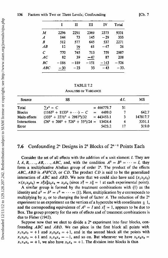
136 Factors with Two or Three Levels; Confounding [Ch. 7
I II III IV Total
M 2296 2291 2369 2375 9331A 144 73 145 —29 333B 512 577 645 537 2271AB 12 79 61 —47 26
C 770 745 713 759 2987AC 82 39 —47 87 208
BC —186 —189 —151 —143 —526
ABC —30 —23 33 —43 —33.
TABLE 7.2
ANALYSIS OF VARIANCE
Source SS d.f. MS
Total ry2 — C = 466779.7 31Blocks (11632 + 1133 2 +••) — C = 4499.0 7 642.7Main effects (3332 + 2271 2 + 2987 2)/32 = 443453.1 3 147817.7Interactions (262 + 208 2 + 5262 + 33 2)/24 = 13404.4 4 3351.1Error 5423.2 17 319.0
7.6 Confounding 2 Designs in 2k Blocks of 2 - k Points Each
Consider the set of all effects with the addition of a unit element I. They areI, A, B, ..., AB, ..., ABC, and, with the condition A 2 = B2 = • • • = I, theyform a multiplicative Abelian group of order 211. The product of the effectsABC, ABD is A 2B2CD, or CD. The product CD is said to be the generalizedinteraction of ABC and ABD. We note that we could also have said (x 1x2x3)x (x1x2x4) = 4xáx3x4 = x3x4 (since xi = xá = 1 at each experimental point).
A similar group is formed by the treatment combinations with (1) as theidentity and a 2 = b2 = c2 = • • • = ( 1). Here, multiplication by a corresponds tomultiplying by x l or to changing the level of factor A. The reduction of the 2 11
experiment to an experiment on the vertices of a hypercube with coordinates ± 1,and the corresponding equivalence of A 2 = I and xi = 1, appears to be due toBox. The group property for the sets of effects and of treatment combinations isdue to Fisher (1942).
Suppose now that we elect to divide a 2n experiment into four blocks, con-founding ABC and ABD. We can place in the first block all points withx1x2x3 = + 1 and x1x2x4 = + 1, and in the second block all the points withx1x2x3 = + 1 and x1x2x4 = — 1, and so on. But whenever we have x1x2x3 =x1x2x4 = + 1, we also have x3x4 = + 1. The division into blocks is thus
Dow
nloa
ded
12/1
1/12
to 1
29.1
28.2
07.2
42. R
edis
trib
utio
n su
bjec
t to
SIA
M li
cens
e or
cop
yrig
ht; s
ee h
ttp://
ww
w.s
iam
.org
/jour
nals
/ojs
a.ph
p

Sec. 7.7] The Allocation of Treatment Combinations to Blocks 137
Block I Block II Block III Block IV
X1X2X3 +1 +1 —1 —1X1X2X4 +1 —1 +1 —1X3X4 +1 —1 —1 +1
Each of the blocks contains 2n -2 points. The contrast in the block totalsI + II — III — IV is the ABC contrast; l — II + III — IV is the ABD contrast.The third degree of freedom between blocks corresponds to I — II — III + IV,which is the CD contrast. No other effects are confounded.
In the general case, let P and Q be two effects. We may divide the 2n designinto four blocks, each of size 2n - 2, by assigning to block I all points which havepositive signs in both the P and Q contrasts; block II contains the points whichhave positive signs in the P contrast and negative signs in the Q contrast, and soon. Then the generalized interaction PQ will also be confounded with blocks,and these will be the only three effects confounded.
If we wish to make eight blocks of size 2i -3, we may take a third effect R(other than PQ). One block will contain all the 2' points that have positivesigns in the P, Q, and R contrasts. The Beven effects confounded will be P, Q,PQ, R, PR, QR, and PQR. In the general case of 2" blocks, we take for thedefining contrasts a set of k independent generators P, Q, R, S,. .. , by whichwe mean k effects such that no one of them is the generalized interaction of anyset of the others. The blocks are then the 2k sets obtained by taking the inter-sections of the sets defined by I = ± P, I = ± Q, I = ± R, I = ± S, .... Thecomplete set of confounded effects consists of the generators and all possiblegeneralized interactions that can be derived from them.
If we add I we obtain a set that includes the identity and is closed under thegroup operation. The set of defining contrasts together with I is thus a sub-group of the group of effects. This subgroup is called the defining contrastsubgroup. It is usually desirable to choose the defining contrasts, if possible, sothat only higher order interactions are confounded. For example, in dividing a 25
experiment into four blocks of eight runs each, we might consider confoundingthe five-factor interaction and one of the four-factor interactions. However,confounding ABCDE and ABCD would be unwise because we should thenautomatically confound their generalized interaction, which is the main effect E.Similarly, choosing ABCDE and ABC as defining contrasts also confounds thetwo-factor interaction DE. A preferable choice of defining contrasts would betwo three-factor interactions and one four-factor interaction such as ABD, ACE,and BCDE. When the block effects are random, the design in which there areone or more main effects confounded is similar to a split-plot design.
7.7 The Allocation of Treatment Combinations to Blocks
We have already mentioned that the blocks are the intersections of the setsdefined by 1 = ±P and 1 = ± Q,.. .. The actual assignment of points to blocks
Dow
nloa
ded
12/1
1/12
to 1
29.1
28.2
07.2
42. R
edis
trib
utio
n su
bjec
t to
SIA
M li
cens
e or
cop
yrig
ht; s
ee h
ttp://
ww
w.s
iam
.org
/jour
nals
/ojs
a.ph
p

138 Factors with Two or Three Levels; Confounding [Ch. 7
is simplified in practice by taking advantage of the fact that the treatmentcombinations form a group. The procedure used is to obtain the principal block,and then to derive the other blocks from it. The principal block is defined to bethe block that contains the base point, or identity element, of the group, (1).
Theorem. The treatment combinations in the principal block form a subgroup ofthe group of all treatment combinations.
PROOF. Let P be a defining contrast and let S. be the set of all treatmentcombinations having an even number of letters (or none) in common with P.Thus, if P were ABC, the set Sp would contain (1), ab, ac, bc, abd, and so on.The set S, is closed and contains (1), for, if ab and ac are both in SP, so is theirproduct bc. Hence, S, is a subgroup. If P contains an even number of letters, S„is the set defined by I = +P. If P contains an odd number of letters, Sp is definedby I = —P. The principal block is the intersection of the sets St,, SQ, ..., and isthus a subgroup. The principal block is sometimes called the intrablock sub-group. 3
If a treatment combination has an even number of letters (or none) in commonwith both P and Q, it also has an even number (or none) in common with PQ.Hence, it is enough to find n — k independent members of the principal block,each having an even number (or none) of letters in common with a set of kgenerators of the defining contrast subgroup, and then to complete the block bytaking products.
The other blocks are obtained by changing the levels of one or more factors.Changing the level of A is equivalent to multiplying each member of the principalblock by a. To change the levels of A and B simultaneously, we multiply eachmember by ab. Thus the other blocks are the cosets of the principal block.
EXAMPLE. Confounding a 25 design in four blocks of eight runs. The definingcontrasts are ABD, ACE, and BCDE.
PrincipalBlock Block II Block III Block IV
(1) d e deade ae ad abd b bde beabe abde ab abdce cde c cdacd ac acde acebcde bce bcd bcabc abcd abce abcde
X4 = —X1X2 +X1X2—X1X2 +X1X2,
X5 = - X1X3 -X1X3 +X1X3 +XJX3
Dow
nloa
ded
12/1
1/12
to 1
29.1
28.2
07.2
42. R
edis
trib
utio
n su
bjec
t to
SIA
M li
cens
e or
cop
yrig
ht; s
ee h
ttp://
ww
w.s
iam
.org
/jour
nals
/ojs
a.ph
p

Sec. 7.81 The Composition of the Defining-Contrast Subgroup 139
The second block is derived by multiplying each member of the principal blockby d, the third by multiplying by e, and the fourth by multiplying by de.
We could also approach the problem of allocation of points in the followingway. The principal block consists of the points for which x1x2x4 = — 1 andx,x3x5 = — 1. Multiplying these equations by x4 and x5, respectively, and notingthat 4 = 4 = 1, we have x4 = — x1x2, x5 = — x1x3 . We can thus obtain theprincipal block by writing down a basic 23 design in the factors A, B, and C, andthen adding the other two factors D and E by putting x4 = — x lx2 and x5 =—xlx3 . Similarly, the second block could be obtained by letting x4 = + x1x2 andx5 = — x1x3 .
7.8 The Composition of the Defining-Contrast Subgroup
In this section we shall temporarily refer to the effects in the defining contrastsubgroup as words. The number of letters in an effect is the length of the word.A word with an odd (even) number of letters is called an odd (even) word. Theproduct of two words is the word for the corresponding generalized interaction.The patterns of word lengths in confounding a 2" design in 2k blocks have beeninvestigated by Brownlee et al. (1948), Burton and Connor (1957), and John(1966a). We shall assume in the remainder of this section that each of the nletters appears in at least one of the words in the subgroup. This eliminates fromour consideration, for example, the design for the 2 3 factorial in two blocks offour runs confounding the main effect A.
The product of two even words, or of two odd words, is an even word. Theproduct of an odd word and an even word is an odd word. The followingnecessary (but not sufficient) conditions can be deduced for the set of 21 — 1words in the defining contrast subgroup:
(i) Each letter appears in exactly 2k -1 words. Hence, if w, is the length of theith word, 1, w, = 2 1n;
(ii)(ii) Either all the words are even, or else exactly 2k -1 of them are odd. Ineither case, the even words together with the identity form a subgroup;
(iii) If one of the words contains all n letters, the remaining words occur inpairs such that the sum of the lengths of the words in any pair is n;
(iv) If one of the words consists of a single letter, the remaining words fallinto pairs, such that the lengths of the words in any pair differ by one.
Suppose that we take any set of k generators. We define a set of parameters:ti denotes the number of letters appearing only in the ith generator; t,; is thenumber of letters that appears only in the ith and jth generators; and so on.The sum of these parameters is t = n. We shall let w(i) denote the length of theith generator and w(i, j) the length of the product of the ith and jth generators.Then
w(1)= t1+112 +...+tras +...,
w(1, 2) = w(1) + w(2) — 2(t12 + t123 + - - •).
Dow
nloa
ded
12/1
1/12
to 1
29.1
28.2
07.2
42. R
edis
trib
utio
n su
bjec
t to
SIA
M li
cens
e or
cop
yrig
ht; s
ee h
ttp://
ww
w.s
iam
.org
/jour
nals
/ojs
a.ph
p

140 Factors with Two or Three Levels; Confounding [Ch. 7
In general let E O(s) t denote the sum of all the t which contain in their sub-scripts an odd number of members from a set S of integers i 1 , i2,..., 1 < i < k.Then, if w(S) denotes the length of the generalized interaction of the i l th, i2th, .. .generators we have
w(S) = 1 t.0(S)
Burton and Connor (1957) derived the formula
1 w2 = 2k - 2(1 t2 + n2^
and showed that properties (i) and (ii) were not sufficient for the existence of aconfounding scheme.
Their example involved trying to block a 2 9 design into 24 blocks, using sevenwords of length 4, six words of length 5, and two words of length 7. We have
w = 72 and so property (i) is satisfied. There is no difficulty in finding a set ofseven four-letter words satisfying property (ii); ABCD, ABEF, and ADFGgenerate such a set.
We note next that 1 w 2 = 360 so that t2 = t = n = 9. It follows thatnine of the t must be unity and the others zero. If such a scheme existed we couldtake as generators the two seven-letter words and two of the five-letter words.We should then have
w(1) + w(2) + w(3) + w(4) = 24.
But
1 W(i) = 4t1234 + 3 1 tht7 + 2 1 t{f + 1 t{.
A total of twenty-four can be obtained only if t1234, all the th1j , and all but two ofthe t;5 are unity.
We can now try to reconstruct a set of generators with these values of t. Oneletter, say A, must be in all four words; another letter, say B, must be in thefirst three words but not the fourth, and so on. There are only two cases to beconsidered: t12 = t34 = 0 and t12 = t13 = 0. In the first case each of thegenerators must have six letters; in the second case w(2) = w(3) = 6. Thus anarrangement with w(1) = w(2) = 7 and w(3) = w(4) = 5 is impossible. Burtonand Connor demonstrated the nonexistence differently, using some other resultsfrom their paper.
7.9 Double Confounding and Quasi-Latin Squares
In a Latin square design p treatments or treatment combinations are applied top2 plots arranged in a square array. The plots are assigned to the treatments in
Dow
nloa
ded
12/1
1/12
to 1
29.1
28.2
07.2
42. R
edis
trib
utio
n su
bjec
t to
SIA
M li
cens
e or
cop
yrig
ht; s
ee h
ttp://
ww
w.s
iam
.org
/jour
nals
/ojs
a.ph
p

Sec. 7.9] Double Confounding and Quasi-Latin Squares 141
such a way that each treatment or treatment combination appears exactly once ineach row and in each column. In consequence, the treatment differences are notconfounded with either the row or the column effects. Yates (1937) introducedthe term quasi-Latin square to denote a design in which more than p treatmentcombinations are used in a p x p square array. There is double confounding.One set of effects is confounded with rows and another set is confounded withcolumns.
In a 4 x 4 square we may have one complete replication of a 2 design or tworeplicates of a 23 factorial. In dividing a 24 design into four blocks of four runseach, we may confound the four-factor interaction and two of the two-factorinteractions, or else two of the three-factor interactions and their product, whichwould be a two-factor interaction. A design in which ABCD, AB, and CDare confounded with columns, and ABC, ACD, and BD are confounded withrows is
(1) bcd abd ac
ab acd d bc
cd b abc ad
abcd a c bd
With this design we can estimate all four main effects and three of the sixtwo-factor interactions, but we have only 2 d.f. that can be used for error. Theseare the 2 d.f. corresponding to ABD and BCD.
When two replicates of the 2 3 factorial are incorporated in one 4 x 4 square,we might choose to have ABC and AB confounded with rows and AC and BCconfounded with columns. There are two ways of achieving this:
BC AC BC AC
abc c b a a b abc cABC
bc ac (1) ab (1) ab ac bcor
(1) ab abc c abc c (1) abAB
a b ac bc bc ac b a
In either case the first two rows and the last two rows are separate replicates.The first two columns and the last two columns also constitute replicates. If,however, the rows and columns are randomized, the design will not in practicehave this nice pattern with runs in the same replicate being in adjacent rows andcolumns. The analysis is similar to that in the example of partial confoundinggiven earlier. Each of the partially confounded effects (the four interactions) isestimated from the two rows (or columns) in which it is not confounded.
Yates gives a design for 26 in an 8 x 8 square confounding ACE, ADF, BDE,BCF, ABCD, ABEF, and CDEF between the rows and ABF, ADE, BCD, CEF,
Dow
nloa
ded
12/1
1/12
to 1
29.1
28.2
07.2
42. R
edis
trib
utio
n su
bjec
t to
SIA
M li
cens
e or
cop
yrig
ht; s
ee h
ttp://
ww
w.s
iam
.org
/jour
nals
/ojs
a.ph
p

142 Factors with Two or Three Levels; Confounding [Ch. 7
ABCE, ACDF, and BDEFbetween the columns. A problem with this design wasnoted by Yates (1948) and was discussed in detail by Grundy and Healy (1950).The difficulty lies in the fact that, when the columns and rows are randomized,there is a considerable probability of obtaining an arrangement in which thecontrast for one of the main effects turns out to be the contrast between diag-onally opposite quarters of the design. This is illustrated in the arrangement thatwe wrote down for the 24 factorial in the 4 x 4 square; the ABD contrast pitsthe four points in the top left quadrant and the four in the bottom right quadrantagainst the points in the other two quadrants.
Yates presents other designs involving the use of several squares. He alsogives quasi-Latin squares for 3n designs and for two replicates of a design withtwo factors at three levels and one at two levels in a 6 x 6 square. He discusses theuse of quasi-Latin squares in split-plot designs, choosing his terminology fromthe weaving of tartans. A design in which main effects are confounded with bothrows and columns is called a plaid square. If main effects are confounded in onlyone direction, we have a half-plaid square.
An example of a half-plaid square for a 2 3 factorial repeated twice, with Aconfounded with rows and BC and ABC confounded with columns is
BC ABC
abc ac a ab
(1) b c bc
a ab abc ac
bc c b (1).
Although we have introduced double confounding with the quasi-Latinsquare, it is not essential that the designs have the same number of rows andcolumns. The following Latin rectangle designs are given by Healy (1951)using four rows and eight columns. The first design consists of four replicates of a23 factorial. Each row consists of a complete replicate, and the treatmentcombinations are arranged within the rows so that only ABC is confound-ed with columns. As the design is written, columns 1 and 2 form a replicateconfounding ABC. So do columns 3 and 4, columns 5 and 6, and columns7 and 8.
(1) a b ab c ac bc abc
ab b a (1) abc bc ac c
ac c abc bc a (1) ab b
bc abc c ac b ab (1) a
Dow
nloa
ded
12/1
1/12
to 1
29.1
28.2
07.2
42. R
edis
trib
utio
n su
bjec
t to
SIA
M li
cens
e or
cop
yrig
ht; s
ee h
ttp://
ww
w.s
iam
.org
/jour
nals
/ojs
a.ph
p

Sec. 7.10] Confounding in 3° Designs 143
In the second design there are two replicates of a 2 4 factorial. Rows 1 and 2,and rows 3 and 4 each comprise a complete replicate of the 2 4 . The first fourcolumns are a complete replicate confounding AB, ACD, and BCD. In the lastfour columns, CD, ABC, and ABD are confounded.
(1) bd ac abcd ab ad bc cd
abc a bcd d acd c abd b
cd bc ad ab (1) bd ac abcd
abd acd b c bcd abc d a
He also gives some designs for the 2 5 factorial in a 4 x 8 rectangle. One ofthese confounds ABC, A DE, and BCDE with rows and A C, DE, ABD, and soon, with columns. The other makes use of fractional factorials, which will bediscussed later.
7.10 Confounding in 3' Designs
We have already mentioned how in the 3 3 experiment the sums of squares foreach of the two-factor interactions and the three-factor interaction can be sub-divided into components with two degrees of freedom. The same procedure leadsto a method of confounding for dividing the twenty-seven points into threeblocks of nine points each. If, for example, AB2C 2 is to be confounded withblocks, we place in the first block the nine points for which x l + 2x2 + 2x3 =_ 0(mod 3); the second block contains the points with x l + 2x2 + 2x3 = 1(mod 3); the third block has x l + 2x2 + 2x3 - 2 (mod 3). The three blocks are
(I) 000, 012, 021, 101, 110, 122, 202, 211, 220;
(II) 002, 011, 020, 100, 112, 121, 201, 210, 222;
(III) 001, 010, 022, 102, 111, 120, 200, 212, 221,
where, for example, a2b1 c 1 is written as 211.Confounding two of the components of the three-factor interaction to obtain
nine blocks of three points each also confounds a main effect. If we take, forexample, the three points for which x l + x2 + x3 = i (mod 3) and xl + 2x2 +2x3 = j (mod 3), we also have 2x1 - i + j (mod 3) or xl - 2(i + j) (mod 3).We can avoid confounding main effects by confounding components of two-factor interactions such as AB, AC, and BC 2 .
Partial confounding can also be used for 3n designs with several replicates.We may take a 3 3 with four replicates and confound each of the four pairs ofdegrees of freedom for the three-factor interaction in one of the replicates. Theanalysis follows the same general pattern as the analysis of the 2 3 example thatwas discussed earlier.
Dow
nloa
ded
12/1
1/12
to 1
29.1
28.2
07.2
42. R
edis
trib
utio
n su
bjec
t to
SIA
M li
cens
e or
cop
yrig
ht; s
ee h
ttp://
ww
w.s
iam
.org
/jour
nals
/ojs
a.ph
p
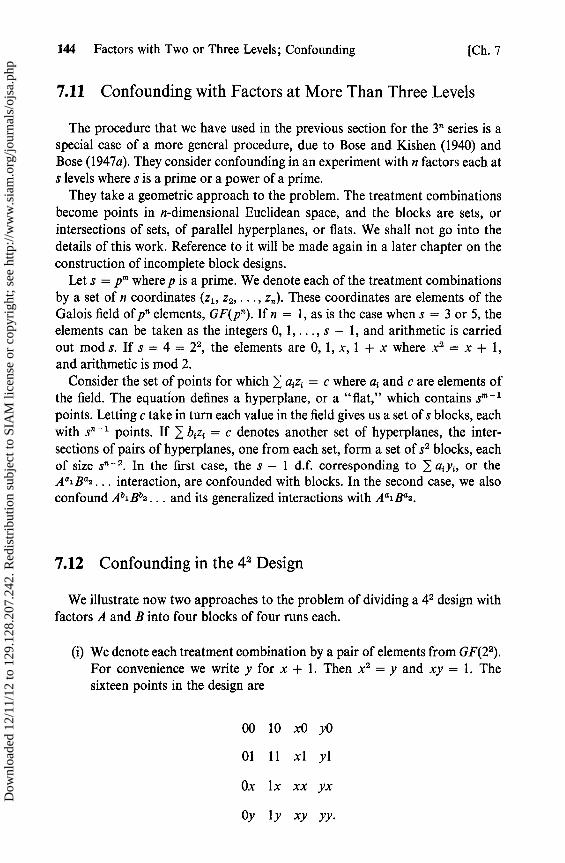
144 Factors with Two or Three Levels; Confounding [Ch. 7
7.11 Confounding with Factors at More Than Three Levels
The procedure that we have used in the previous section for the 3n series is aspecial case of a more general procedure, due to Bose and Kishen (1940) andBose (1947a). They consider confounding in an experiment with n factors each ats levels where s is a prime or a power of a prime.
They take a geometric approach to the problem. The treatment combinationsbecome points in n-dimensional Euclidean space, and the blocks are sets, orintersections of sets, of parallel hyperplanes, or flats. We shall not go into thedetails of this work. Reference to it will be made again in a later chapter on theconstruction of incomplete block designs.
Let s = pm where p is a prime. We denote each of the treatment combinationsby a set of n coordinates (z 1 , z2f ... , za). These coordinates are elements of theGalois field ofpn elements, GF(pn). If n = 1, as is the case when s = 3 or 5, theelements can be taken as the integers 0, 1, ..., s — 1, and arithmetic is carriedout mod s. If s = 4 = 22, the elements are 0, 1, x, 1 + x where x2 = x + 1,and arithmetic is mod 2.
Consider the set of points for which 1 a,z{ = c where at and c are elements ofthe field. The equation defines a hyperplane, or a "flat," which contains sm-1
points. Letting c take in turn each value in the field gives us a set of s blocks, eachwith sn -1 points. If 1 b;z, = c denotes another set of hyperplanes, the inter-sections of pairs of hyperplanes, one from each set, form a set of s 2 blocks, eachof size sti -2 . In the first case, the s — 1 d.f. corresponding to ai yi, or theAa1Ba2... interaction, are confounded with blocks. In the second case, we alsoconfound Ab1Bb2... and its generalized interactions with Aa1Ba2.
7.12 Confounding in the 4 2 Design
We illustrate now two approaches to the problem of dividing a 4 2 design withfactors A and B into four blocks of four runs each.
(i) We denote each treatment combination by a pair of elements from GF(22).For convenience we write y for x + 1. Then x 2 = y and xy = 1. Thesixteen points in the design are
00 10 xO y0
01 11 xl yl
Ox lx xx yx
Oy ly xy yy.
Dow
nloa
ded
12/1
1/12
to 1
29.1
28.2
07.2
42. R
edis
trib
utio
n su
bjec
t to
SIA
M li
cens
e or
cop
yrig
ht; s
ee h
ttp://
ww
w.s
iam
.org
/jour
nals
/ojs
a.ph
p

Sec. 7.13] Confounding in Other Factorial Experiments 145
There are 9 degrees of freedom for AB interaction. We elect to confoundwhat might be called the ABx component by taking as blocks the flatszl + xz2 = c. The blocks are
z l +xz2 = 0 1 x y
00 Oy 01 Ox
ly 10 lx 11
xl xx xO xy
yx yl yy y0.
(ii) We may replace each four-level factor by two pseudofactors, each at twolevels, A by P and Q, B by R and S. Let the coordinate one denote apseudofactor at its high level and zero denote it at its low level. Thepoints are
0000 1000 0100 1100
0010 1010 0110 1101
0001 1001 0101 1110
0011 1011 0111 1111
This really amounts to replacing 0, 1, x, and y in the previous representa-tion by 00, 10, 01, and 11, respectively.
The three degrees of freedom for A correspond to the main effects P and Qand the interaction PQ. The main effects of B are R, S, and RS. The other nineinteractions between the pseudofactors correspond to the interaction AB. Wecan now elect to split the 2 design into four blocks confounding PQR, QRS, andPS. This method will give the same blocks as the previous method.
7.13 Confounding in Other Factorial Experiments
The methods described in this chapter can be applied, although not so easily,to factorial experiments in which the factors do not all have the same number oflevels. If some of the factors have two levels and the others have four levels, theconfounding can be achieved by the use of pseudofactors, which has just beendescribed. Yates (1937) discusses confounding in designs with some three-levelfactors and some four-level factors. Binet et al. (1955) consider dividing a singlereplicate of a design with factors at several levels into blocks.
Dow
nloa
ded
12/1
1/12
to 1
29.1
28.2
07.2
42. R
edis
trib
utio
n su
bjec
t to
SIA
M li
cens
e or
cop
yrig
ht; s
ee h
ttp://
ww
w.s
iam
.org
/jour
nals
/ojs
a.ph
p

146 Factors with Two or Three Levels; Counfounding [Ch. 7
Exercises
1. Apply Yates' algorithm to the following set of data for a 2 4 experiment:
(1) 3.96 c 3.71 d 4.53 cd 4.52a 4.05 ac 3.87 ad 4.69 acd 4.72b 2.71 bc 2.67 bd 3.01 bcd 3.32ab 2.94 abc 3.02 abd 3.37 abcd 3.53
2. Use the algorithm to evaluate the contrasts and obtain the analysis of variancetable for the 3 3 design given as an example in Chapter 5.
3. Devise an algorithm in the style of Yates for calculating the contrasts in a22 x 3 design. Use it to carry out the analysis of variance for the followingdesign which has two levels of P, two levels of N, and three levels of K.
Ko K1 KZ
No N1 No N1 No N1
Po 23 36 25 46 25 31
P1 34 28 19 54 19 38
4. The data in exercise 1 were actually taken from a 22 x 4 experiment [Raese andDecker (1966)]. Factors C and D correspond to the factor with four levels. Usethe results of exercise 1 to obtain the analysis of variance table for the 2 2 x 4design.
5. In the section on partial confounding we considered the example of a 23 designwith four replicates, each divided into two blocks of four points each. Prove thatthe estimates we obtained are actually the least squares estimates.
6. Prove the necessity of the four conditions on the words in the defining contrastsubgroup given at the beginning of the section on the composition of that group.
7. Find the principal block when the 2 8 design is split into blocks of sixteen runseach, using the defining contrast subgroup generated by ABCD, ABEF, ABGH,ACEG.
8. Derive the quasifactorial design for a 2 6 design in an 8 x 8 square by Yates,which was mentioned in the text.
9. Derive a design for a 25 factorial in a 4 x 8 rectangle, confounding ABC, ADE,BCDE with rows and AC, DE, ABD with columns.
10. Obtain the partially confounded design for a 3 3 factorial with four replicates,each in three blocks of nine points each. Confound ABC with blocks in the firstreplicate, ABC 2 in the second, AB 2C in the third, and AB 2C 2 in the fourth.
11. A reasonable procedure when a plot is missing in a 2n design is to replace it bya value which makes the highest order interaction zero. Apply this technique tothe data of exercise 1, assuming bc to be missing. What is the variance of theestimate of an effect when a missing plot is included?
12. (Continuation). In the 2n design the highest order interaction has only onecontrast. However, in a 3" design the highest order interaction has 2n degrees
Dow
nloa
ded
12/1
1/12
to 1
29.1
28.2
07.2
42. R
edis
trib
utio
n su
bjec
t to
SIA
M li
cens
e or
cop
yrig
ht; s
ee h
ttp://
ww
w.s
iam
.org
/jour
nals
/ojs
a.ph
p

Exercises 147
of freedom; thus, there are 2" orthogonal contrasts, each of which might beequated to zero to calculate a missing value. A less ambiguous procedurewould be to omit all the highest order interaction terms from the model and usethe procedure of the earlier chapters. Investigate this for the 3 3 experiment ofexercise 2, assuming that the point 012 is missing.
Dow
nloa
ded
12/1
1/12
to 1
29.1
28.2
07.2
42. R
edis
trib
utio
n su
bjec
t to
SIA
M li
cens
e or
cop
yrig
ht; s
ee h
ttp://
ww
w.s
iam
.org
/jour
nals
/ojs
a.ph
p

CHAPTER 8
Fractions of2n Factorial
Designs
As the number of factors in a 2n design increases, the number of points soonoutgrows the facilities and budgets of most experimenters. The full 28 experiment calls for 256 runs. Only eight of the degrees of freedom correspond to maineffects, and twenty-eight to two-factor interactions. The remaining 219degrees offreedom correspond to interactions involving three or more factors. If thesehigher order interactions are all negligible, the experimenter has 219 degrees offreedom for error, which is more than he really needs for an adequate estimate.On the other hand, he hasto make 256 runs to estimate only 8 + 28 effects, andonly 14 per cent of the degrees of freedom are used for estimation.
We have already seen how Latin squares can be used to estimate the maineffects in a p3 factorial experiment with only p2 runs. Graeco- Latin squares andhyper-Graeco-Latin squares result in even greater savings, but at the cost ofassuming that some of the interactions do not exist.
This chapter is devoted to an investigation of fractions of 2n designs. One ofthe fractions that will be discussed can be derived from a Latin square of side 2,either
I 2
2 Ior
2 1
1 2.
If we let rows represent the levels of A, columns the levels of B, and I and 2 thelevels of C, we have two four-point fractions of the 23 design: (1), be, ab, ae, andb, e, a, abc. These are half replicates of the 23 design, or 23
-1 designs, from which
the main effects A, B, and C are estimable, if we neglect their interactions. The2n - " fractions, or 1{2" fractions of Z" designs were introduced by Finney (1945).
148
Dow
nloa
ded
12/1
1/12
to 1
29.1
28.2
07.2
42. R
edis
trib
utio
n su
bjec
t to
SIA
M li
cens
e or
cop
yrig
ht; s
ee h
ttp://
ww
w.s
iam
.org
/jour
nals
/ojs
a.ph
p

Sec. 8.1 ] The 2n - k Fractional Factorials 149
They will be the topic of the first part of the chapter, after which some otherfractions will be discuseed.
Fractional factorials are commonly used in industrial experimentation whereruns are expensive and where an acceptable prior estimate of the variance isavailable. They may also be used for screening experiments. These are experi-ments performed in the early stages of an investigation in which many factorsare considered, most of which may turn out to have little or no effect upon theresponse under investigation. The purpose of the screening experiment is toscreen several factors with the purpose of spotting those factors, if any, that haveappreciable effects. The factors that seem to be interesting are then investigatedmore closely in subsequent experiments. The emphasis is not so much uponestimating the effects with small variance, but upon finding out which of thefactors merit further study. We shall assume throughout most of this chapterthat the experimenter is interested in estimating the main effects, and perhaps thetwo-factor interactions; that he is prepared to assume before carrying out theexperiment that the higher order interactions are negligible; and that he is notparticularly concerned with using the actual experiment to provide himself withan estimate of the variance. The emphasis will therefore be on finding smallexperiments in which a high percentage of the degrees of freedom are used forestimation. In these small experiments there will be few degrees of freedom forerror even if higher order interactions are used, and it will be assumed that theexperimenter has some prior estimate of the error variance. Daniel (1959) hasintroduced a graphical method for deciding which effects in a 2n factorial aresignificant when there is no estimate of error. If there is no prior estimateavailable such graphical procedures seem to be the only recourse.
8.1 The 2' FractionalFractional Factorials
When in the previous chapter we divided the 2 5 design into four blocks ofeight runs, each block constituted a quarter replicate, or a 25 - 2 fraction. Theterm 2n - k fraction or (1/2k)th replicate is used to describe only those sets of2n-k treatment combinations that could occur in the same block when thecomplete factorial is divided into 2k blocks confounding exactly 2k — 1 effectsin the manner derived in the previous chapter. Thus we may define a 2' -k
fraction as a set of 2n -k different points which constitute a subgroup of thegroup of treatment combinations, or a coset of such a subgroup. This definitionthrows very little light upon the nature of fractional factorials and their impor-tance. Henceforth we shall regard a subgroup as a trivial coset of itself, and usethe term coset to embrace both the subgroup itself and the other cosets.
The first fraction listed (the principal block) was the fraction defined byI = — ABD = —ACE = + BCDE. The other fractions in order were defined byI= +ABD=—ACE=—BCDE,I=—ABD=+ACE=—BCDE,and I=+ABD = +ACE = +BCDE. The four fractions are said to belong to the samefamily. The term principal fraction has been used in the literature in two different
Dow
nloa
ded
12/1
1/12
to 1
29.1
28.2
07.2
42. R
edis
trib
utio
n su
bjec
t to
SIA
M li
cens
e or
cop
yrig
ht; s
ee h
ttp://
ww
w.s
iam
.org
/jour
nals
/ojs
a.ph
p

150 Fractions of 2n Factorial Designs [Ch. 8
senses and we shall refrain from employing it here. Some authors use it todenote the fraction containing (1) by analogy with the term principal block.Box and Hunter (1961) use it to denote the fraction for which the definingcontrasts all have positive signs; in our example that would be the fractioncontaining de, a, be, abd, cd, ace, bc, and abcde. We now consider that fraction inmore detail.
For each treatment combination in the fraction the relationship 1 = x 1x2x4 =
x 1x3x5 = x2x3x4x5 holds. Multiplying by x 1 and recalling that xi = 1, we have
xl = x2x4 = x3x5 = x1x2x3x4x5
at each point so that A, BD, CE, and ABCDE are indistinguishable. The foureffects A, BD, CE, and ABCDE are said to constitute an alias set and to bealiased (or confounded) with each other. The alias sets are the cosets of thedefining contrast subgroup (which is sometimes called the alias subgroup inthis context). There are 2n - k alias sets (including the subgroup itself) and eachset has 2k members. Each effect is aliased with the effects in the same alias setbut with no others.
If the elements of the vector of effects F3 are written by order of alias sets sothat P' = (PO, P124, P1359 P2345, P13 P24, P35, P12345, ...) the cross-product matrixX'X in the normai equations consists of square matrices 8J4 along the maindiagonal and zeros elsewhere. The rank of X'X is 8. A matrix of full rank isobtained by choosing one effect from each of the alias sets and striking out theremaining rows and columns. If, therefore, we were to assume a restricted modelwhich included the mean, the five main effects, either BC or DE, and either CDor BE, but no other terms, the corresponding least squares equations would havea unique set of solutions.
The A contrast from this fraction is
(a + abd + ace + abcde — de — be — cd — bc).
Its expectation is 8(fl1 + P24 + f35 + P12345), so that when we use the contrastto estimate A we are actually estimating A + BD + CE + ABCDE. The otherfractions give chains A ± BD ± CE ± ABCDE, with the signs correspondingto the signs of the defining contrasts. The full set of alias chains is
I +ABD+ ACE +BCDE
B + AD + ABCE + CDE
C + ABCD + AE + BDE
BC + ACD + ABE + DE
A + BD + CE + ABCDE
AB + D + BCE + ACDE
AC + BCD + E + ABDE
ABC + CD + BE + ADE
For A to be estimated we must assume that BD, CE, and ABCDE are all zero.If we plan to use this fraction with the intention of estimating A we must decidea priori that we are going to ignore the other three interactions. The prior
Dow
nloa
ded
12/1
1/12
to 1
29.1
28.2
07.2
42. R
edis
trib
utio
n su
bjec
t to
SIA
M li
cens
e or
cop
yrig
ht; s
ee h
ttp://
ww
w.s
iam
.org
/jour
nals
/ojs
a.ph
p

Sec. 8.2] The Classification of Fractions 151
decision to ignore the five-factor interaction will cause little concern, but it maynot be reasonable to assume without further investigation that the two-factorinteractions BD and CE are negligible. If these two particular interactions arethe only ones that concern the experimenter, he can avoid the difficulty bychoosing a different fraction such as one of the 2 5 - 2 defined by I = ± ABC =± A DE = ± BCDE. The two interactions will then be aliased with each other,but not with any of the main effects. There is not a quarter replicate from whichthe mean, the five main effects, BD and CE can all be estimated. If, on theother hand, the experimenter is not willing to declare prior to carrying out hisexperiment that any of the two-factor interactions can be ignored, he cannotestimate without bias the five main effects from any 2 5-2 fraction. In that case heis going to have to perform a larger experiment or to omit one of the factors.
8.2 The Classification of Fractions
We have seen that in the use of fractional replicates it is necessary to assumea priori that certain effects are zero. It is a common practice in industrialexperimentation to make the blanket assumption in the absence of priorinformation to the contrary that all interactions that involve three or morefactors can be ignored. We shall make that assumption in this chapter. Aninteraction which is taken to be zero in this way will be said to be suppressed.We shall sometimes suppress the two-factor interactions also, and considerestimating only the main effects. It will be convenient to use the abbreviation2 f.i. for the expression two factor interaction.
An effect will be said to be estimable if, and only if, there is a contrast in thedata which has for its expectation the particular effect biased only by othereffects which we choose to suppress. The effect being estimated is said to bealiased with the effects that were suppressed. Designs in which main effects arealiased with each other are of no interest. The remaining designs are divided intoseveral classes.
One method of classification has three classes:
(i) Main effects only designs. These are fractions in which some of the maineffects are aliased with 2 f.i. and are estimable only when those 2 f.i. aresuppressed;
(ii) Main effects clear plans. These are fractions in which al] the main effectsare estimable whether the 2 f.i. are suppressed or not, but some of the 2f.i. are aliased with each other;
(iii) 2 f.i. clear plans. These are fractions in which all the main effects and allthe 2 f.i. are estimable.
These classes were originally called types A, B, and B' by Box and Wilson(1951). Box and Hunter used the terras resolution III, resolution IV, andresolution V. Daniel (1962) called them three-, four-, and five-letter plans. The
Dow
nloa
ded
12/1
1/12
to 1
29.1
28.2
07.2
42. R
edis
trib
utio
n su
bjec
t to
SIA
M li
cens
e or
cop
yrig
ht; s
ee h
ttp://
ww
w.s
iam
.org
/jour
nals
/ojs
a.ph
p

152 Fractions of 2n Factorial Designs [Ch. 8
last two terminologies are in common use. The justification for Daniel's nomen-clature becomes clear when the alias sets are considered. If one of the definingcontrasts is a three-letter word, say ABC, then A is aliased with BC, B with AC,and C with AB; the three main effects are estimable only if the three 2 f.i. aresuppressed. With ABCD as a defining contrast, A is aliased with BCD, but ABis aliased with CD. With a five-letter word ABCDE, the main effects and 2 f.i.are all aliased only with higher order interactions.
We shall use the following definition of the resolution of a fractional factorial,which is applicable to other fractions as well as the 2n - ' series. An interactioninvolving t factors will be called a tth order effect; main effects are first-ordereffects. Let t be any integer.
A design is said to be of resolution (2t + 1) if it satisfies the condition that alleffects of order t or less are estimable whenever all effects of order higher than tare suppressed.
A design is said to be of resolution 2t if all effects of order (t — 1) or less areestimable whenever all effects of order (t + 1) or higher are suppressed.
8.3 Some 2n - k Fractions
The 23 -1 DesignThe smallest usable 2n - k fraction is the 23-1 consisting of four points. Two
such designs are useful: one, defined by I = ABC, contains the four points,a, b, c, and abc; the other, defined by I = — ABC, consists of (1), ab, ac, and bc.Both these designs are three-letter plans. Each main effect is aliased with atwo-factor interaction. In the first of these half replicates the estimates of themain effects are
= (abc + a — b — c)/4 with expectation A + BC;
= (abc + b — a — c)/4 with expectation B + AC;
P3 = (abc + c — a — b)/4 with expectation C + AB.
The variance of each estimate is a2/4.In the traditional one-at-a-time experiment, which appeals to some experi-
menters, each factor is varied in turn while the other factors are maintained attheir low levels. With three factors this design consists of the four points (1),a, b, and c. It is interesting to compare this design with the half replicates. Eachuses four points to estimate the mean and the three main effects. However, theestimate of the main effect A, for example, from the one-at-a-time experiment isp 1 = (a — (1))/2 with expectation A — AB — AC + ABC and variance o2/2.The 2 -1 fraction thus provides an estimate which has a smaller variance andwhich is biased by fewer interactions.
The one-at-a-time experiment should not, however, be dismissed completelybecause of its relative inefficiency. It is attractive to some experimenters in
Dow
nloa
ded
12/1
1/12
to 1
29.1
28.2
07.2
42. R
edis
trib
utio
n su
bjec
t to
SIA
M li
cens
e or
cop
yrig
ht; s
ee h
ttp://
ww
w.s
iam
.org
/jour
nals
/ojs
a.ph
p
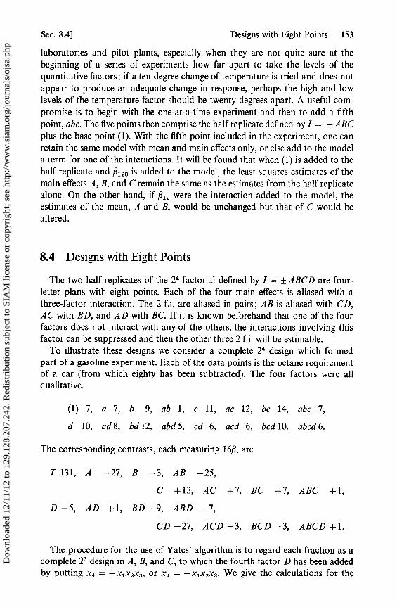
Sec. 8.4] Designs with Eight Points 153
laboratories and pilot plants, especially when they are not quite sure at thebeginning of a series of experiments how far apart to take the levels of thequantitative factors; if a ten-degree change of temperature is tried and does notappear to produce an adequate change in response, perhaps the high and lowlevels of the temperature factor should be twenty degrees apart. A useful com-promise is to begin with the one-at-a-time experiment and then to add a fifthpoint, abc. The five points then comprise the half replicate defined by I = + ABCplus the base point (1). With the fifth point included in the experiment, one canretain the same model with mean and main effects only, or else add to the modela term for one of the interactions. It will be found that when (1) is added to thehalf replicate and P123 is added to the model, the least squares estimates of themain effects A, B, and C remain the same as the estimates from the half replicatealone. On the other hand, if P12 were the interaction added to the model, theestimates of the mean, A and B, would be unchanged but that of C would bealtered.
8.4 Designs with Eight Points
The two half replicates of the 24 factorial defined by I = ± ABCD are four-letter plans with eight points. Each óf the four main effects is aliased with athree-factor interaction. The 2 f.i. are aliased in pairs; AB is aliased with CD,AC with BD, and AD with BC. If it is known beforehand that one of the fourfactors does not interact with any of the others, the interactions involving thisfactor can be suppressed and then the other three 2 f.i. will be estimable.
To illustrate these designs we consider a complete 2 design which formedpart of a gasoline experiment. Each of the data points is the octane requirementof a car (from which eighty has been subtracted). The four factors were allqualitative.
(1) 7, a 7, b 9, ab 1, c 11, ac 12, bc 14, abc 7,
d 10, ad 8, bd 12, abd 5, cd 6, acd 6, bcd 10, abcd 6.
The corresponding contrasts, each measuring 16p, are
T 131, A -27, B -3, AB -25,
C +13, AC +7, BC +7, ABC +1,
D -5, AD +1, BD +9, ABD -7,
CD-27, ACD + 3, BCD + 3, ABCD + 1.
The procedure for the use of Yates' algorithm is to regard each fraction as acomplete 2 design in A, B, and C, to which the fourth factor D has been addedby putting x4 = + x1x2x3i or x4 = - x 1x2x3 . We give the calculations for the
Dow
nloa
ded
12/1
1/12
to 1
29.1
28.2
07.2
42. R
edis
trib
utio
n su
bjec
t to
SIA
M li
cens
e or
cop
yrig
ht; s
ee h
ttp://
ww
w.s
iam
.org
/jour
nals
/ojs
a.ph
p

154 Fractions of 2n Factorial Designs [Ch. 8
two half replicates. The fourth column of figures in each section is the column ofcontrasts; these figures, which estimate 8fl, should be compared with one half ofthe values of the contrasts for the complete design.
I = +ABCD
(1) 7 15 28 66ad 8 13 38 —12 Abd 12 18 —10 0 Bab 1 20 —2 —26 AB + CDcd 6 1 —2 10 C
ac 12 —11 2 8 AC + BDbc 14 6 —12 4 BC + ADabcd 6 —8 —14 —2 D
I = —ABCD
d 10 17 31 65a 7 14 34 —15 A
9 17 —7 —3 Babd 5 17 —8 1 AB — CDc 11 —3 —3 3 C
acd 6 —4 0 —1 AC—BD bcd 10 —5 —1 3 BC — ADabc 7 —3 2 3 —D
The last contrast in each table is the ABC contrast. In the first fraction thiscontrast estimates 8(ABC + D); suppressing ABC we have 8$4 = — 2. In thesecond half replicate the contrast estimates 8(ABC — D), so that we have—8 4 = 3, or 8 4 = — 3.
It should also be noted that adding the values of the contrasts in the two halfreplicates gives the values for the complete design. Thus the A contrast for thecomplete factorial is —27 = (-12) + (-15) ; the AB contrast is —26 + 1 =— 25, and the CD contrast is — 26 — 1 = — 27. We are reminded in the secondhalf replicate that it is not wise to conclude, just because the estimate of AB —CD is —1, that both AB and CD are small. Although there is no mathematicaljustification for it, some scientists would as a practical matter be prepared, asDaniel (1962) has pointed out, to assume for example in the first half replicatethat, since the A and C effects are large and the B and D effects are small, therelatively large size of the AC + BD contrast can be attributed to the ACinteraction rather'than the BD interaction. This procedure, lacking as it does afirm mathematical basis, can lead to pitfalls unless the scientist has a consider-able amount of prior information about the probable relationships between thefactors.
If we add to the first of these half replicates a fifth factor E by puttingx5 = x1x2, we have the 25-2 design defined by 1 = ABCD = ABE = CDE.
Dow
nloa
ded
12/1
1/12
to 1
29.1
28.2
07.2
42. R
edis
trib
utio
n su
bjec
t to
SIA
M li
cens
e or
cop
yrig
ht; s
ee h
ttp://
ww
w.s
iam
.org
/jour
nals
/ojs
a.ph
p

Sec. 8.5] Designs with Sixteen Points 155
This resolution III design consists of the points e, ad, bd, abe, cde, ac, bc, abcde,and is similar to the 2 5 - 2 designs that were mentioned earlier.
Adding F by putting xs = x1x3 gives the 26-3 design defined by I = ABCD =ABE = CDE = ACF = BDF = BCEF = ADEF, which consists of the pointsef, ad, bdf, abe, cde, acf, bc, abcdef.
Finally, we may add a seventh factor by letting x 7 = x2x3 and obtain efg, adg,bdf, abe, cde, acf, bcg, abcdefg. The defining contrast subgroup for this fractionis generated by ABCD, ABE, ACF, and BCG. The alias chains for main effectsand 2 f.i. are
A+BE+CF+DG
B+AE+CG+DF
C+AF+BG+DE
D+AG+BF+CE
E+AB+CD+FG
F+AC+BD+EG
G+AD+BC+EF
A three-letter plan for 2t t -1 factors in 2n runs can always be constructed in thisway by starting with a basic 2n design and then adding new factors by equatingthem to interactions.
8.5 Designs with Sixteen Points
The half replicates of the 2 5 design defined by I = + ABCDE or by I=—ABCDE are designs of resolution V. Each main effect is aliased with a four-factor interaction; each 2 f.i. is aliased with a three-factor interaction. There arefive main effects and ten 2 f.i. Thus there are as many effects to be estimated asthere are degrees of freedom. A fraction in which each degree of freedom is usedto estimate an effect is said to be saturated. Daniel (1956) introduced the termsdegree-of-freedom efficiency and variance efficiency for a fractional factorial.The variance efficiency of a fraction is obtained by comparing the average of thevariances of the estimates of the effects to the smallest variance that could behoped for with factors at the levels ± 1. For a main effect such as A, the minimumvariance of the estimate $ is obtained when half the points are at x, = +1 andhalf are at x l = —1; the variance is then V(P1) = a2IN. The 2' fractionsall have 100 per cent variance efficiency. We shall discuss later some non-orthogonal fractions which have lower efficiencies. The degree-of-freedomefficiency is the ratio of the number of effects estimated to the number of degreesof freedom in the design. The 2 5 -1 fractions have 100 per cent degree-of-freedomefficiency.
Dow
nloa
ded
12/1
1/12
to 1
29.1
28.2
07.2
42. R
edis
trib
utio
n su
bjec
t to
SIA
M li
cens
e or
cop
yrig
ht; s
ee h
ttp://
ww
w.s
iam
.org
/jour
nals
/ojs
a.ph
p

156 Fractions of 2' Factorial Designs [Ch. 8
The half replicate defined by I = — ABCDE consists of the sixteen points
(1), ae, be, ab, ce, ac, bc, abce, de, ad, bd, abde, cd, acde, bcde, abcd.
The complementary half replicate, defined by I = + ABCDE, contains alltreatment combinations with an odd number of letters.
Four-letter plans for six, seven, or eight factors can be obtained by startingwith a basic 24 design and adding the other factors by putting E = ABC,F = ABD, G = ACD, and H = BCD. The design for all eight factors consistsof the points
(1), aefg, befh, abgh, cegh, acfh, bcfg, abce,
dfgh, adeh, bdeg, abdf, cdef, acdg, bcdh, abcdefgh.
The defining contrast subgroup is generated by ABCE, ABDF, ACDG, andBCDH; each defining contrast contains an even number of letters.
Designs like this can also be obtained by the important method of foldingover. Suppose that we begin with a resolution III design, the 2 7 - 4 design witheight points presented in the previous section. We can regard it as a 2 6 - 5 designin which all the runs were made at the low level of the factor H, and add thegenerator —H to the defining contrast subgroup. The folding-over processconsists of repeating each run with the levels of every factor changed. Thus,folding over efg gives abcdh. The design is
efg, adg, bdf, abe, cde, acf, bcg, abcdefg,
abcdh, bcefh, acegh, cdfgh, abfgh, bdegh, adefh, h.
For the first eight points we have x1x2x5 = x1x3x6 = x2x3x7 = — x8 = + 1; forthe second eight points we have x1x2x5 = x1x3x6 = x2X3x7 = —X8 = — 1. Forthe whole set of sixteen points we have (x 1 x2x5)(x 1x3x6) = (x 1x2x5)(x2x3x7) =
(x1x2x5)( — x8) ` (x1x3x6)(x2x3x7) = (x1x3x6)( — x8) = (x2x3x7)( — x8) = + 1, andalso x 1 X2x3x4 = 1.
Thus x2x3x5x6 = x1x3x5x7 = —x 1 x2x5x6 = • • _ + 1 and the generators ofthe fraction are BCFG, ABEG, —ABEH, ABCD.
In general, folding over will convert any design of resolution III into a designof resolution IV or higher. The defining contrasts for the combined design arethose defining contrasts of the original fraction that contain an even number ofletters, and, since there are no two-factor interactions in that set, they all containfour letters or more. The original 2" fractionfraction has 2k -1 — 1 defining contrastswith an even number of letters and 2k -1 with an odd number. In the comple-mentary fraction obtained by folding over, the signs of each of the odd definingcontrasts are changed, and the signs of each of the even contrasts are unaltered.It also follows that folding over a resolution V design produces a design ofresolution VI or higher.
Dow
nloa
ded
12/1
1/12
to 1
29.1
28.2
07.2
42. R
edis
trib
utio
n su
bjec
t to
SIA
M li
cens
e or
cop
yrig
ht; s
ee h
ttp://
ww
w.s
iam
.org
/jour
nals
/ojs
a.ph
p

Sec. 8.6] Other 2" - ' Fractions of Resolution V 157
Folding over can also be considered from the point of view of breaking chainsof aliases. Since the three-letter defining contrasts change signs in the secondfraction, the 2 f.i. change signs in those alias chains which include main effects.Thus, in our example, the alias chain for A in the first eight points (consideringonly main effects and 2 f.i.) is A + BE + CF + DG — AH, while the corre-sponding alias chain in the second set is A — BE — CF — DG + AH. The Acontrast from the first eight points gives an estimate of ft + P25 + P36 +P47 — P12. From the second eight points we have an estimate of fl — p„ —P3s — P47 + . Adding them gives an estimate of 22 1 .
Another possibility is to take a design of resolution III and repeat it, changingonly the level of A without adding the extra factor H. This gives a design inwhich A and all the 2 f.i. which contain A are estimable, biased only by inter-actions involving three or more factors. In our example the design would be
efg, adg, bdf, abe, cde, acf, bcg, abcdefg,
aefg, dg, abdf, be, acde, cf, abcg, bcdefg.
The set of defining contrasts for the combined design consists of all the definingcontrasts of the original design which do not contain A. The alias chainscontaining A are A + BE + CF + DG and A — BE — CF — DG. The aliaschains containing AB are AB + E + FG + CD and AB — E — FG — CD.
8.6 Other 2n - k Fractions of Resolution V
For six factors the smallest 2n - k fraction of resolution V is a half replicate.This can be defined either by the six-factor interaction, I = ± ABCDEF, or byany one of the five-factor interactions. We would usually prefer one of the halvesdefined by the six-factor interaction, because the main effects would be aliasedwith five-factor interactions and the 2 f.i. with four-factor interactions.
For seven or eight factors, sixty-four points are needed. For seven factors thisrequires a half replicate. With eight factors we can obtain a suitable quarterreplicate with two five-letter words and a six-letter word in the defining con-trasts, for example, I = ABCDE = ABFGH = CDEFGH.
2n - k fractions of resolution V for nine, ten, or eleven factors call for 128 pointseach. Examples of suitable sets of defining contrasts are
29-2 : 1= ABCDEF = ABCGHJ = DEFGHJ;210-3 : 1= ABCDEF = ABCGHJ = ABDEGHK;
211-4 : 1= ABCDEF = ABFJK = AEFGKL = ACEHL.
The first is a design of resolution VI. In the last two fractions only sets ofgenerators for the defining contrast subgroups are given. For twelve or morefactors at least 256 runs are needed. A set of generators for a 212 -4 design ofresolution V is ABCDJK, ABEFJL, ADEGLM, ABGHKL.
Dow
nloa
ded
12/1
1/12
to 1
29.1
28.2
07.2
42. R
edis
trib
utio
n su
bjec
t to
SIA
M li
cens
e or
cop
yrig
ht; s
ee h
ttp://
ww
w.s
iam
.org
/jour
nals
/ojs
a.ph
p
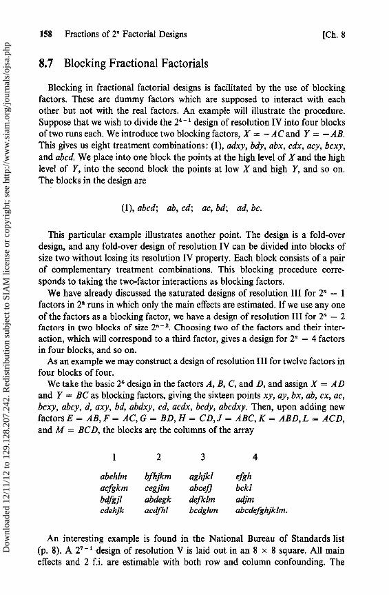
158 Fractions of 2n Factorial Designs [Ch. 8
8.7 Blocking Fractional Factorials
Blocking in fractional factorial designs is facilitated by the use of blockingfactors. These are dummy factors which are supposed to interact with eachother but not with the real factors. An example will illustrate the procedure.Suppose that we wish to divide the 2 4 -1 design of resolution IV into four blocksof two runs each. We introduce two blocking factors, X = — AC and Y = — AB.This gives us eight treatment combinations: (1), adxy, bdy, abx, cdx, acy, bcxy,and abcd. We place into one block the points at the high level of X and the highlevel of Y, into the second block the points at low X and high Y, and so on.The blocks in the design are
(1), abcd; ab, cd; ac, bd; ad, bc.
This particular example illustrates another point. The design is a fold-overdesign, and any fold-over design of resolution IV can be divided into blocks ofsize two without losing its resolution IV property. Each block consists of a pairof complementary treatment combinations. This blocking procedure corre-sponds to taking the two-factor interactions as blocking factors.
We have already discussed the saturated designs of resolution III for 2n — 1factors in 2n runs in which only the main effects are estimated. If we use any oneof the factors as a blocking factor, we have a design of resolution III for 2n — 2factors in two blocks of size 2'' -2 . Choosing two of the factors and their inter-action, which will correspond to a third factor, gives a design for 2n — 4 factorsin four blocks, and so on.
As an example we may construct a design of resolution III for twelve factors infour blocks of four.
We take the basic 24 design in the factors A, B, C, and D, and assign X = ADand Y = BC as blocking factors, giving the sixteen points xy, ay, bx, ab, cx, ac,bcxy, abcy, d, axy, bd, abdxy, cd, acdx, bcdy, abcdxy. Then, upon adding newfactors E = AB, F = AC, G = BD, H = CD, J = ABC, K = ABD, L = ACD,and M = BCD, the blocks are the columns of the array
4
abehlm bfhjkm aghjkl efghacfgkm cegjlm abcefj bcklbdfgjl abdegk defklm adjmcdehjk acdfhl bcdghm abcdefghjklm.
An interesting example is found in the National Bureau of Standards list(p. 8). A 2 -1 design of resolution V is laid out in an 8 x 8 square. All maineffects and 2 f.i. are estimable with both row and column confounding. The
Dow
nloa
ded
12/1
1/12
to 1
29.1
28.2
07.2
42. R
edis
trib
utio
n su
bjec
t to
SIA
M li
cens
e or
cop
yrig
ht; s
ee h
ttp://
ww
w.s
iam
.org
/jour
nals
/ojs
a.ph
p
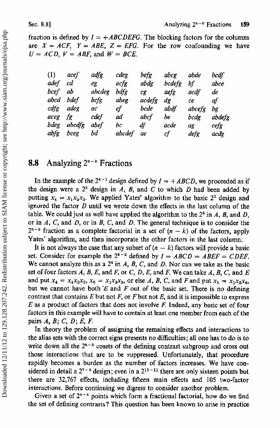
Sec. 8.8] Analyzing 2n -' Fractions 159
fraction is defined by I = + ABCDEFG. The blocking factors for the columnsare X = ACF, Y = ABE, Z = EFG. For the row confounding we haveU = ACD, V = ABF, and W = BCE.
(1) acef adfg cdeg befg abcg abde bcdfadef cd eg acfg abdg bcdefg bf abcebcef ab abcdeg bdfg cg aefg acdf deabcd bdef bcfg abeg acdefg dg ce afcdfg adeg ac ef bcde abdf abcefg bgaceg fg cdef ad abcf be bcdg abdefgbdeg abcdfg abef bc df acde ag cefgabfg bceg bd abcdef ae cf defg acdg
8.8 Analyzing 2 - k Fractions
In the example of the 2 4 -1 design defined by I = + ABCD, we proceeded as ifthe design were a 2 3 design in A, B, and C to which D had been added byputting x4 = x1x2x3 . We applied Yates' algorithm to the basic 2 3 design andignored the factor D until we wrote down the effects in the last column of thetable. We could just as well have applied the algorithm to the 2 3 in A, B, and D,or in A, C, and D, or in B, C, and D. The general technique is to consider the2n - k fraction as a complete factorial in a set of (n — k) of the factors, applyYates' algorithm, and then incorporate the other factors in the last column.
It is not always the case that any subset of (n — k) factors will provide a basicset. Consider for example the 2 8 - 2 defined by I = ABCD = ABEF = CDEF.We cannot analyze this as a 2 in A, B, C, and D. Nor can we take as the basicset of four factors A, B, E, and F, or C, D, E, and F. We can take A, B, C, and Eand put x4 = x1x2x3 , x6 = x 1x2x5 , or else A, B, C, and F and put x5 = x1x2x6 ,
but we cannot have both 1E and F out of the basic set. There is no definingcontrast that contains E but not F, or F but not E, and it is impossible to expressE as a product of factors that does not involve F. Indeed, any basic set of fourfactors in this example will have to contain at least one member from each of thepairs A, B; C, D; E, F.
In theory the problem of assigning the remaining effects and interactions tothe alias sets with the correct signs presents no difficulties; all one has to do is towrite down all the 2n - k cosets of the defining contrast subgroup and cross outthose interactions that are to be suppressed. Unfortunately, that procedurerapidly becomes a burden as the number of factors increases. We have con-sidered in detail a 2 - 4 design; even in a 215 -11 there are only sixteen points butthere are 32,767 effects, including fifteen main effects and 105 two-factorinteractions. Before continuing we digress to consider another problem.
Given a set of 2" - k points which form a fractional factorial, how do we findthe set of defining contraets? This question has been known to arise in practice
Dow
nloa
ded
12/1
1/12
to 1
29.1
28.2
07.2
42. R
edis
trib
utio
n su
bjec
t to
SIA
M li
cens
e or
cop
yrig
ht; s
ee h
ttp://
ww
w.s
iam
.org
/jour
nals
/ojs
a.ph
p

160 Fractions of 2" Factorial Designs [Ch. 8
when, by the time the experiment has been completed, the information on howthe fraction was constructed has been lost. It has been discuseed by Nelder(1963). The method of solving the problems presented in this section is due toMargolin (1967).
We assume that we have already found by inspection a basic set of factors orIetters. Margolin gives a simple method of doing this and calls the letters in thebasic set live letters and the others dead. It will be helpful to consider an example.Consider the eight-point fraction bc, acde, abdf, ef, ag, bdeg, cdfg, abcefg. E, F,and G are a set of live letters. The first step is to find a defining contrast thatcontains A and some of the live letters, but no other dead letters. We shall thendo the same for B, C, and D, and the four contrasts will be a set of generators forthe defining-contrast subgroup. These contrasts are called the special definingcontrasts for the dead letters. Margolin gives two rules.
To determine the sign of the special contrast for any dead letter in the definingrelationship of the fraction, we examine the treatment combination in which all(n — k) of the live factors are at their high levels. If, at this point, the particulardead factor is also at its high level, then the special contrast for that factor has apositive sign. If the factor is at its low level, the contrast has a negative sign. Inthe example the special contrasts for A, B, and C have positive signs; that for Dhas a negative sign.
We now find which live factors appear in the special contrast of the deadfactor being considered. We consider each live factor in turn and look at twopoints, the point at which all the live factors are at their low levels, and thepoint at which the particular live factor is at its high level and the others are attheir low levels. If the dead factor is at the same level in both points, then the livefactor does not appear in the special contrast; if the levels are different, the livefactor is present.
In the example we consider first the special contrast for A. We have alreadyestablished that it has a positive sign. The point at which E, F, and G are allat their low levels is bc. In each of the points acde, abdf, ag, A is at its highlevel and therefore all three letters, E, F, and G, appear in the special contrastfor A, which is thus AEFG. The other special contrasts are BEG, CFG, and—DEF.
We return now to the problem of the aliases. We have A = EFG, B = EG,C = FG, and D = — EF. We next write down the Beven sets of three effects in thelive 23 that have the identity for their generalized interaction: (E, F, EF — D),(E, G, EG = B), (E, FG = C, EFG = A), (F, FG, G), (F, EG, EFG), (G, EF,EFG), (EF, EG, FG). When the interactions are expressed as dead factors, theproducts give the set of three letter defining contrasts,
— DEF, BEG, ACE, CFG, ABF, — ADG, — BCD,
and the alias chains for the main effects and 2 f.i. follow immediately, A + CE +BF — DG, B + EG + AF — CD, and so on.
Dow
nloa
ded
12/1
1/12
to 1
29.1
28.2
07.2
42. R
edis
trib
utio
n su
bjec
t to
SIA
M li
cens
e or
cop
yrig
ht; s
ee h
ttp://
ww
w.s
iam
.org
/jour
nals
/ojs
a.ph
p

Sec. 8.9] Designs Obtained by Omitting 2n - k Fractions 161
8.9 Designs Obtained by Omitting 2n - k Fractions
We begin by considering an example. In the 2 4- k series there is nothingbetween the half replicate of resolution IV, from which the main effects can beestimated, and the complete factorial with sixteen points. The main effects andthe six 2 f.i. call for only ten degrees of freedom. Can we estimate all of themwith only twelve runs? John (1961a) showed that there were two ways in whichthis could be done by omitting a quarter replicate from the complete design.The problem arose in a practical situation: an experiment had to be plannedwith four factors at two levels each and there was only enough raw materialavailable to make twelve runs. How might those twelve runs best be chosen?
Consider the family of quarter replicates defined by
(i) I = +AB = +ACD = +BCD d, ab, c, abcd;
(ii) I = —AB = +ACD = —BCD bd, a, bc, acd;
(iii) I = +AB = —ACD = —BCD (1), abd, cd, abc;
(iv) I = —AB = —ACD = +BCD b, ad, bcd, ac;
and suppose that we omit the first of them. The remaining fractions form threeoverlapping half replicates
(ii) + (iii) I = —BCD, (ii) + (iv) I = —AB, (iii) + (iv) I = —ACD.
We can estimate A from (ii) + (iii) sine there A is aliased with ABCD; A isnot, however, estimable from either of the other two half replicates. B is estim-able from (iii) + (iv); C, D, and CD from (ii) + (iv); AC and AD from (ii) +(iii); BC and BD from (iii) + (iv). We shall see later that these are the leastsquares estimates. AB is estimable from both (ii) + (iii) and (iii) + (iv); theleast squares estimate is the average of these two estimates.
We recall the model
E(y) = Po + $ix= + $1xx1 + .. .t s ^
that we presented before, and again consider the normal equations X'Y =X'XO. The alias sets for the quarter replicates are I, AB, ACD, BCD; A, B, CD,ABCD; C, ABC, AD, BD; and AC, BC, D, ABD. We write the elements of theparameter vector f3 in that order: P ' = (9p, P12, $134, $234, Nl, N2, P349 $1234, • • • )•
The cross-product matrix, X'X, for the complete desigr. is 24I4 . The cross-product matrix for the omitted fraction (i) consists of submatrices 4J 4 along themain diagonal and zeros elsewhere. The cross-product matrix for the twelve-point design is the differente between these two matrices and consists of sub-matrices 16I4 — 4J 4 along the diagonal. Each of these submatrices is of rank 3.When we suppress from the model the higher order interactions and strike out
Dow
nloa
ded
12/1
1/12
to 1
29.1
28.2
07.2
42. R
edis
trib
utio
n su
bjec
t to
SIA
M li
cens
e or
cop
yrig
ht; s
ee h
ttp://
ww
w.s
iam
.org
/jour
nals
/ojs
a.ph
p
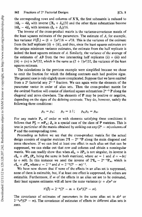
162 Fractions of 2n Factorial Designs [Ch. 8
the corresponding rows and columns of X'X, the first submatrix is reduced to16I2 — 4J2 with inverse (2I2 + J2)/32 and the other three submatrices become16I3 — 4J3 with inverses (I3 + J3)/16.
The inverse of the cross-product matrix is the variance-covariance matrix ofthe least squares estimates of the parameters. The estimate of A, for example,has variance V(P 1) = (1 + 1)x2/16 = a2/8. This is the variance of the estimatefrom the half replicate (ii) + (iii), and thus, since the least squares estimates arethe unique minimum variance estimates, the estimate from the half replicate isindeed the least squares estimate of A. Similarly, the variance of the average ofthe estimates of AB from the two intersetting half replicates (ii) + (iii) and(iii) + (iv) is 3a2/32, which is the same as (2 + 1)a2/32, the variance of the leastsquares estimate.
The calculations in the previous example were simplified because we choseto omit the fraction for which the defining contrasts each had positive signs.The general case is only slightly more complicated. Suppose that we have omittedfrom a 2n factorial any 2n - k fraction. We can again write the elements of theparameter vector in order of alias sets. Then the cross-product matrix forthe omitted fraction will consist of identical square submatrices 2n - k P along thediagonal and zeros elsewhere. The elements of P may be positive or negative,depending on the signs of the defining contrasts. They do, however, satisfy thefollowing three conditions:
R^ = P>i; p = ± 1; Ph>Pi> = Pni.
For any matrix Pm of order m with elements satisfying these conditions itfollows that P, = mPm ; Jm is a special case of the class of P matrices. This istrue in particular of the matrix obtained by striking out any (2k — m) columns ofP and the corresponding rows.
Proceeding as before we see that the cross-product matrix for the actualdesign consists of singular matrices 2nI — 2n - kP along the main diagonal andzeros elsewhere. If we can find at least one effect in each alias set that can besuppressed, we can strike out that row and column and obtain a nonsingularmatrix. We can readily show that when aIm + bPm is not singular, its inverse iscIm + dPm (Pm being the same in both matrices), where ac = 1 and d = — bc/(a + mb). In this instante we need the inverse of 2'I m — 2n - kPm , which iscIm + dPm where c = 2 - n and d = 2 - n(2k — m) 1 .
We have now shown that if none of the effects in an alias set is suppressed,none of them is estimable, but, if at least one effect is suppressed, the others areestimable. Furthermore, if m of the effects in an alias set are to be estimated,their least squares estimates will all have the same variance (c + d)a2 or
V(P) = 2 - n(2k — m + 1 )a2/(2k — m).
The covariance of estimates of parameters in the same alias set is doe or2 - n02/(2k — m). The covariance of estimates of effects in different alias sets iszero
Dow
nloa
ded
12/1
1/12
to 1
29.1
28.2
07.2
42. R
edis
trib
utio
n su
bjec
t to
SIA
M li
cens
e or
cop
yrig
ht; s
ee h
ttp://
ww
w.s
iam
.org
/jour
nals
/ojs
a.ph
p

Sec. 8.101 Three-Quarter Replicates 163
We now turn to the problem of finding estimates that have these variances.If we can do so, they will be the unique least squares estimates, and the co-variances will look after themselves. Now that we have established the variance-covariance matrix of the estimates, there will be no loss of generality if wesimplify matters by assuming that each of the defining contrasts in the omittedfraction has a positive sign. Suppose that it is defined by I = P = Q =PQ = • • • . The actual design then consists of 2k — 1 overlapping half replicatesdefined by I = —P, I = — Q, I = —PQ, and so on. Each pair of these halfreplicates has a quarter in common: for example, the half replicates defined byI = —P and by I = — Q both share the points for which I = —P =
—Q = +PQ.
Let S be an effect that is to be estimated. In the half replicate defined byI = —P, S is aliased with PS, and if PS is suppressed, S can be estimated fromthat half replicate. If 2" — m of the effects in the same alias set as S are sup-pressed, S is estimable from 2k — m overlapping half replicates. Each of theseestimates has variance 2 -(n -1)a2 ; their covariance is 2 - no2 . Let P denote theaverage of these estimates. Then
V(P) = (2k — m) -2{(2k — m)2 -(n-1) + (2k — m)(2k — m — 1)2 - n}a2
= 2 - n(2k — m + 1 )a2/(2k — m),
which is the same as the variance of the least squares estimate.We have thus established the following method of calculating the least
squares estimates of effects. To obtain the least squares estimate of an effect S,take the estimates of S from each of the half replicates in which it is estimableand average them.
8.10 Three-Quarter Replicates
The simplest designs of this type are the three-quarter replicates or 3(2n -2)
designs [John (1962)]. These fractions are obtained by omitting one of thequarters from a full factorial and are said to be defined by the missing quarter.Thus the twelve-point design just presented is the 3(24-2) design defined byI = AB = ACD = BCD. Had the set of points b, ad, bcd, ac been omittedinstead, we should have had the 3(2 4 2) defined by I = — AB = —ACD =BCD. We can add other factors to 3(2n -2) designs and obtain 3(2n - k) designs.
The smallest of these designs has six points. We can omit from the 2 3 factorialany one of the quarters defined by I = ± AB = ± AC = ± BC. These are (1),abc; a, bc; b, ac; ab, c. The alias sets are I, AB, AC, BC and A, B, C, ABC. Eachof the main effects is estimated from the half replicate in which it is aliased withABC. The 2 f.i. and the mean are hopelessly confounded with each other. Thedesign is a resolution IV design. The variance efficiency of the estimates of themain effects is 8/12 = 2/3.
This design can be made into a 3(25 - 3) fraction of resolution 111 by addingtwo more factors, D and E. They are equated to any two of the interactions
Dow
nloa
ded
12/1
1/12
to 1
29.1
28.2
07.2
42. R
edis
trib
utio
n su
bjec
t to
SIA
M li
cens
e or
cop
yrig
ht; s
ee h
ttp://
ww
w.s
iam
.org
/jour
nals
/ojs
a.ph
p

164 Fractions of 2° Factorial Designs [Ch. 8
± AB, ± AC, ± BC. Suppose that we let D = —AB and E = — BC. Then D andE are estimated from the half replicates in which they are aliased with A C. If weomit the quarter defined by I = — AB = —AC = +BC, the six points are(1), abc, bde, acde, abe, ce.A and D are estimated from the half replicate defined by I = — BC. The A
contrast is abe + acde — ce — bde. The D contrast is acde + bde — abe — ce.B and the general mean are estimated from the half replicate defined by I =+AC. The B contrast is abc + bde — (1) — acde; 4P0 = (1) + abc + bde +acde. C and E are estimated from the half replicate defined by I = + AB. The Ccontrast is abc + ce — (1) — abe; the E contrast is abe + ce — (1) — abc.
In general, any 3(2' -2) fraction can be made into a design of resolution IIIfor 3(2n -2) — 1 factors. New factors are assigned to interactions in such a waythat three of the effects in each alias set correspond to main effects and one isleft over. Each main effect is then estimated from the half replicate in which it isaliased with the suppressed effect that is left over. In this way we can convert the3(24-2) fraction mentioned earlier into a design of resolution III for elevenfactors. We can let E = AB, F = ACD, G = CD, H = ABC, J = AD,K = AC, M = BC with BCD, ABCD, BD, and ABD left over. The design wouldthen be
(ii) bdfhk afghm bcfjm acdfgjk
(iii) egjkm abdej cdegh abcehkm
(iv) bghjk adhjm bcdgm ack,
where (ii), (iii), and (iv) refer to the original quarters. The main effects B, E, H,and M are estimated from (iii) + (iv); D, F, G, and J are estimated from (ii) and(iv); the mean, A, C, and K are estimated from (ii) + (iii).
The design that we gave earlier is not the only 3(2 4-2) of resolution III. Wecould also have omitted one of the quarters defined by I = ± A = ± BCD =± ABCD. Some experimenters might prefer to use this fraction because in it theone effect that is estimated from two half replicates is the main effect A ratherthan a 2 f.i.
The 3(24-2) defined by I = AB = AC = BC and the 3(24 - 2) defined byI = AB = CD = ABCD are also of interest. Neither is of resolution V, thelatter having an alias set, AC, BC, AD, BD, which contains only two-factorinteractions. Both, however, are of resolution IV and can be made to accommo-date six factors. Consider in particular the first design. The alias sets are I, AB,AC, BC; AD, BD, CD, ABCD; A, B, C, ABC; and b, ABD, ACD, BCD. Wecan add two more factors, E and F, by setting them equal to two of the inter-actions ± ABD, ± ACD, ± BCD. The main effects will be clear of 2 f.i.; the2 f.i. will be hopelessly confounded. If we let E = +ABD and F = +ACD,the twelve points will be
aef bcef be ace abf cf
bcd ad acdf bdf cde abde.
Dow
nloa
ded
12/1
1/12
to 1
29.1
28.2
07.2
42. R
edis
trib
utio
n su
bjec
t to
SIA
M li
cens
e or
cop
yrig
ht; s
ee h
ttp://
ww
w.s
iam
.org
/jour
nals
/ojs
a.ph
p

Sec. 8.11 ] The 3(25 - 2) Designs 165
It should be noted that this is a fold-over design and that it can be divided intosix blocks of two runs each without losing its resolution IV property. The blocksare the columns of the array in which we have written the points.
This illustrates a general procedure for obtaining a resolution IV design for3(2' - 3) factors in 3(2 11 - 2) runs. We take a 3(2 11 - 2) fraction defined by omittinga quarter replicate in which every defining contrast contains an even number ofletters. The alias sets then consist either of four effects each with an evennumber of letters, or else of four effects each with an odd number of letters.The new factors are added by equating them to odd interactions, leaving oneover in each alias set. The 2 f.i. will then all have an even number of letters, andso they will not appear in the same alias sets as the main effects.
8.11 The 3(25_2) Designs
We have already seen that the 2 -1 fractions defined by I = ± ABCDE aresaturated fractions of resolution V with sixteen points. It is interesting toinvestigate the gains, if any, that can be made by using twenty-four points.To what extent can we, by a suitable choice of twenty-four points, obtáin betterestimates, i.e., estimates with smaller variances? It is not immediately obviousthat any improvement can be made, apart from the fact that we shall have anestimate of error with 8 d.f. from the actual data; after all, in a three-quarterreplicate some of the effects are only estimable from a single half replicate,which is what we have in the 2 5 -1 designs.
Apart from permutations of the letters and choices of sign in the definingcontrasts of the omitted fraction, there are only six 3(25 _2) fractions of resolutionV. The defining contrasts and alias sets for them are given in the table on page166.
Designs 4 and 5 have the property that each alias set contains exactly two ofthe effects that are to be estimated. In these designs we have V(ftn) = V (Ph) =3a/64; the half replicate gives V(h) = V(Pht) = c2 / 16. Designs 1, 2, and 3 eachhave three alias sets with only one suppressed effect. In each case these alias setscontain main effects, which means that in these designs several of the maineffects are only estimated from single half replicates. Taking the extra points hasnot improved the precision of the estimates of those main effects.
When we consider blocking, the differences between the designs become moreapparent. The choice of the blocking variables in one of these designs affectsnot only the number of blocks but also their sizes [John (1964b)]. When one ofthe defining contrasts is used as a blocking factor in a 3(2n -2) design, we havetwo blocks; one of these is a half replicate and the other is the remainingquarter. If one of the other effects is used, we have two blocks of equal size.If two effects in the same alias set are used for blocking, their product, which is adefining contrast, is also a blocking factor. Thus, if two of the defining con-trasts are blocking factors, so is the third, and the blocks are the quarters; if oneof the other alias sets contains two blocking factors, there are four blocks, two
Dow
nloa
ded
12/1
1/12
to 1
29.1
28.2
07.2
42. R
edis
trib
utio
n su
bjec
t to
SIA
M li
cens
e or
cop
yrig
ht; s
ee h
ttp://
ww
w.s
iam
.org
/jour
nals
/ojs
a.ph
p
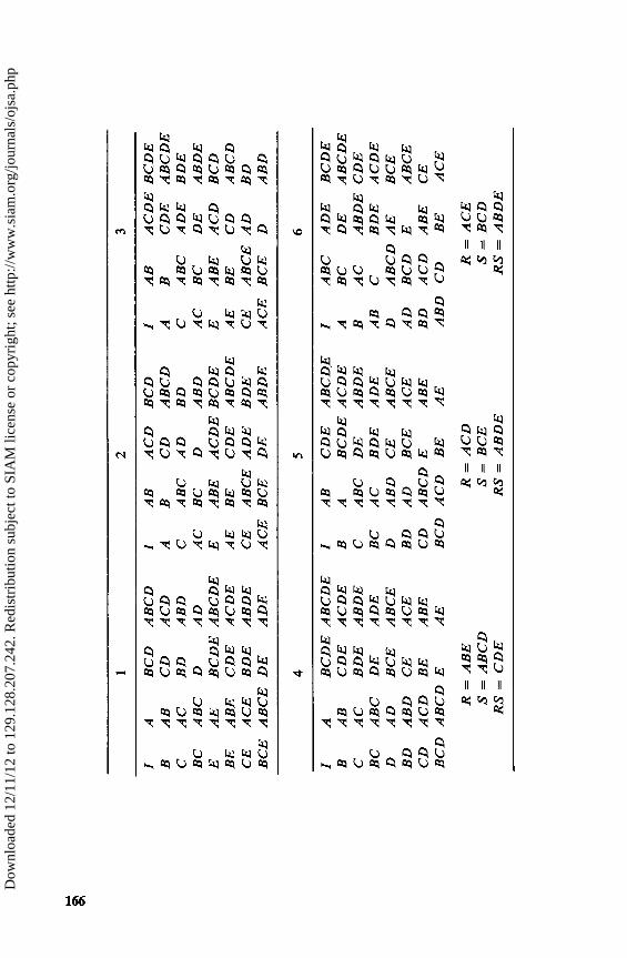
I-'
~
12
3
IA
BC
DA
BC
DI
AB
AC
DB
CD
IA
BA
CD
EB
CD
EB
AB
CD
AC
DA
BC
DA
BC
DA
BC
DE
AB
CD
EC
AC
BD
AB
DC
AB
CA
DB
DC
AB
CA
DE
BD
EB
CA
BC
DA
DA
CB
CD
AB
DA
CB
CD
EA
BD
EE
AE
BC
DE
AB
CD
EE
AB
EA
CD
EB
CD
EE
AB
EA
CD
BC
DB
EA
BE
CD
EA
CD
EA
EB
EC
DE
AB
CD
EA
EB
EC
DA
BC
DC
EA
CE
BD
EA
BD
EC
EA
BC
EA
DE
BD
EC
EA
BC
EA
DB
DB
CE
AB
CE
DE
AD
EA
CE
BC
ED
EA
BD
EA
CE
BC
ED
AB
D
45
6
IA
BC
DE
AB
CD
EI
AB
CD
EA
BC
D.E
IA
BC
AD
EB
CD
EB
AB
CD
EA
CD
EB
AB
CD
EA
CD
EA
BC
DE
AB
CD
EC
AC
BD
EA
BD
EC
AB
CD
EA
BD
EB
AC
AB
DE
CD
EB
CA
BC
DE
AD
EB
CA
CB
DE
AD
EA
BC
BD
EA
CD
ED
AD
BC
EA
BC
ED
AB
DC
EA
BC
ED
AB
CD
AE
BC
EB
DA
BD
CE
AC
EB
DA
DB
CE
AC
EA
DB
CD
EA
BC
EC
DA
CD
BE
AB
EC
DA
BC
DE
AB
EB
DA
CD
AB
EC
EB
CD
AB
CD
EA
EB
CD
AC
DB
EA
EA
BD
CD
BE
AC
E
R=
AB
ER
=A
CD
R=
AC
ES
=A
BC
DS
=B
CE
S=
BC
DR
S=
CD
ER
S=
AB
DE
RS
=A
BD
E
Dow
nloa
ded
12/1
1/12
to 1
29.1
28.2
07.2
42. R
edis
trib
utio
n su
bjec
t to
SIA
M li
cens
e or
cop
yrig
ht; s
ee h
ttp://
ww
w.s
iam
.org
/jour
nals
/ojs
a.ph
p

Sec. 8.13] Adding Fractions 167
with 2n - 2 points each and two with 2n - 3 points each. Finally, if two effects indifferent alias sets, neither of which is a defining contrast, are used for blocking,their product is in a third alias set and we have four blocks of equal size. In allcases, for an effect to be estimable there must be a suppressed effect in the alias setin addition to any blocking factors.
Designs 4, 5, and 6 can each be blocked into four blocks of six points each byusing as blocking factors the three factors R, S, and RS, which are given in eachcase. Design 6 can be run in separate quarters. Designs 1, 2, and 3 may be splitinto blocks of sizes 8, 8, 4, and 4. A particularly interesting property of designs 4and 5 is that they may be blocked, using ABCDE, into the half replicate definedby I = ± ABCDE and the remaining quarter. An implication of this is that wemay elect to complete either of these designs if, after the half replicate has beenrun, we find ourselves able to make an additional eight runs. Alternatively,we may choose to run the half replicate first anyway, as a precaution againstfinding ourselves in a situation in which we are not able to complete the twenty-four point sequence.
8.12 Some 3(2'1- k) Designs of Resolution V
The smallest 2 8 - k design of resolution V is a quarter replicate with sixty-fourpoints. The following 3(28-4) fraction has resolution V in forty-eight points.Omitting one of the factors gives a design of resolution V for Beven factors inforty-eight points. We omit from the complete 26 factorial the quarter defined byI = ABE = CDF = ABCDEF, and add new factors by putting G = ABCDand H = A CEF. The three quarters of the design are
(i) fg, aef, befh, abfgh, c, aceg, bcegh, abch, dh, adegh, bdeg, abd, cdfgh,acdefh, bcdef, and abcdfg;
(ii) eg, a, bh, abegh, cef, acfg, bcfgh, abcefh, defh, adfgh, bdfg, abdef, cdegh,acdh, bcd, and abcdeg;
(iii) gh, aeh, be, abg, cfh, acefgh, bcefg, abcf, df, adefg, bdefgh, abdfh, cdg,acde, bcdeh, and abcdgh.
The three quarters may be used as blocks.With ninety-six points we can obtain a design of resolution V for eleven
factors. This is achieved by omitting from the 2 factorial the quarter defined byI = AB = CDEFG = ABCDEFG and adding new factors H = ABDEF,J = ABCEG, K = AEFG, and L = BCDE. The alias sets are presented inJohn (1969).
8.13 Adding Fractions
The three-quarter replicate can fust as well be obtained by adding a quarterreplicate to a half replicate. The addition of other fractions to a half replicate
Dow
nloa
ded
12/1
1/12
to 1
29.1
28.2
07.2
42. R
edis
trib
utio
n su
bjec
t to
SIA
M li
cens
e or
cop
yrig
ht; s
ee h
ttp://
ww
w.s
iam
.org
/jour
nals
/ojs
a.ph
p

168 Fractions of 23 Factorial Designs [Ch. 8
does not, however, give such neat results. There are some useful designs that canbe obtained in this way and in them, too, the least squares estimates of theestimable effects can be pieced together from the estimates from the constituentfractions. We shall illustrate the procedure by an example and state the resultsfor the general case.
Suppose that we take a 2n 1 design defined by I = —P where P is some effect,and add to it the 2n - 3 fraction defined by I = P = Q = PQ = R = PR =QR = PQR. Let S be some other effect. The alias set, which contains S, consistsof S, PS, QS, PQS, RS, PRS, QRS, and PQRS. This alias set is composed offour pairs of effects, such as S, PS, which are themselves aliased in the halfreplicate. If one of the effects in each pair is suppressed, the other four effectscan be estimated from the half replicate without the need for any additionalpoints. The extra points are needed only to break chains of aliases, such asS— PS, when neither effect is suppressed.
As an example, suppose that in a 2 4 factorial we take the half replicate definedby I = —ABCD and add the 2 - 3 defined by 1= ABCD = A = BCD = B =ACD = AB = CD. There are two alias sets:
M, ABCD; A, BCD; B, ACD; AB, CD;
C, ABD; AC, BD; BC, AD; D, ABC.
As usual, we suppress the interactions with three or four factors.We shall call a pair of effects such as S and PS a nonnegligible pair if neither
S nor PS is suppressed. The first alias set contains one nonnegligible pairAB, CD; the second set has two such pairs A C, BD and AD, BC. The points inthe design are
abc, abd, a, acd, b, bcd, c, d, ab, abcd.
We can take the extra eighth replicate (ab, abcd) and combine it in turn witheach of the eighths in the original half replicate that have the same definingcontrasts. This will give us four overlapping 2 - 2 fractions:
1= A = B = AB, abc, abd, ab, abcd;
I = A = CD = ACD, a, acd, ab, abcd;
I = B = CD = BCD, b, bcd, ab, abcd;
1= AB = ACD = BCD, c, d, ab, abcd.
From the first of these quarters we have an estimate of CD: CD =(ab + abcd — abc — abd)/4. In the half replicate the CD contrast gives anestimate of CD — AB: (a + acd + b + bcd — abc — abd — c — d)/8. If wesubtract this from the estimate CD, we obtain an estimate of AB:
ÁB=(2ab+2abcd—abc— abd —a— acd —b— bcd +c+d)/8.
Dow
nloa
ded
12/1
1/12
to 1
29.1
28.2
07.2
42. R
edis
trib
utio
n su
bjec
t to
SIA
M li
cens
e or
cop
yrig
ht; s
ee h
ttp://
ww
w.s
iam
.org
/jour
nals
/ojs
a.ph
p

Sec. 8.13] Adding Fractions 169
Both CD and AB have variances a2/4. Also the mean, A, and B are estimablefrom the original half replicate. Thus all the effects in the first alias set that arenot suppressed are estimable.
We find in considering the submatrix of the cross-product matrix that if wedelete the suppressed effects and write the remaining effects in the order M, A, B,AB, and CD the submatrix is
4I3 + J3E3,2 lU 1 = 2
E2,3 8I2 — 3J2)
where Em ,,, is a matrix of m rows and n columns with every element unity. Thecorresponding covariance submatrix is
_ 4 2I3—E
Ui( —E I2 + 3J2)1 = 2
This shows that V(P0) = V(P1) = V(j2) = a2/8 and V(P12) = V(P34) =and so the estimates that we have given for M, A, B, AB, and CD are the leastsquares estimates.
On the other hand, the cross-product submatrix for the other alias set is
4I2 + J2 J2 J2
U2 = 2 J2 8I2 — 3J2J2
J2J2 812-3J2
where the first two columns correspond to C and D, the next two to the non-negligible pair AC and BD, and the last two to the nonnegligible pair AD andBC. The matrix U2 is singular. The main effects C and D are estimable from theoriginal half replicate, but the addition of the two extra points does not breakeither of the chains AC — BD or AD — BC.
The results in the general case where a 2' - k fraction is added to a disjoint halfreplicate are as follows:
(i) Any effects that are estimable in the half replicate are estimable in theaugmented design (the worst that can happen is that the estimates willbe the same);
(ii) If an alias set contains more than one nonnegligible pair, the onlyestimable effects that can be estimated are those that are estimated in thehalf replicate, and the estimates from the half replicate are the leastsquares estimates of the effects from all 2n -1 + 2n - k points;
(iii) If an alias set contains only one nonnegligible pair and, also, m pairswith one effect suppressed and one to be estimated (m < 2k -1 — 1),all the effects are estimable.
Dow
nloa
ded
12/1
1/12
to 1
29.1
28.2
07.2
42. R
edis
trib
utio
n su
bjec
t to
SIA
M li
cens
e or
cop
yrig
ht; s
ee h
ttp://
ww
w.s
iam
.org
/jour
nals
/ojs
a.ph
p

170 Fractions of 2" Factorial Designs [Ch. 8
In the last case, when m < 21c -1 — 1, and in the case in which an alias set hasno nonnegligible pairs, the least squares estimates are not simply the estimatesfrom the half replicate. They may be found by following the procedures derivedin John (1966b) or by using the results obtained by Plackett (1950).
This technique of adding fractions may be used to obtain a design of resolutionV for seven factors in thirty-six runs. The smallest such 27 - k fraction hassixty-four runs; any of the half replicates having as the defining contrast aninteraction involving five, six, or seven factors will sufface. A design with forty-eight runs is obtained by using a 3(2 7 - 3) fraction; one can, for example, omit thequarter defined by I = ABC = DEF = ABCDEF from the complete 26 designand add a new factor by putting G = ABCD. The thirty-six point design is a sub-set of the forty-eight point fraction. It is obtained as follows. We add to the26-1 defined by I = — ABCDEF the four-point fraction generated by I =+ABCDEF = +ABDEF = —ABC = +BCDEF = ...; the seventh factor isagain added by putting G = ABCD.
Also of interest is an eighty-point design of resolution V for nine factors.This is obtained by adding to the 2 -1 defined by I = — AB the 27 - 3 definedby I = AB = CDEFG = ABCDEFG = ACF = BCF = ADEG = BDEG andthen putting H = AEFG and J = BCDE.
8.14 Nested Fractions
We have already mentioned that one of the differences between industrial andagricultural experimentation is that in the former the runs can often be made insequence. Advantage can be taken of this in planning an experimental strategy.There is also a disadvantage because experiments may by misfortune be termi-nated before all the runs have been made. The designer would be prudent toanticipate such risks.
We expect the size of an experiment to be determined in the planning stageby budgetary considerations or, perhaps on some occasions, by calculationsinvolving the power of the t or F tests. Very often, however, time plays animportant part because the scientist is allotted a pilot plant for only a limitedtime. For example, he might have the use of a pilot plant for two weeks, or forten working days. If he can make two runs a day, and if he allows the first dayto set up his equipment, that gives him eighteen runs. A 2 4 design followed bytwo check points on the last day might be appropriate.
But what are the consequences if something goes wrong with the machineryand three days are lost while a pump is being replaced? Such misfortunes arenot uncommon. The loss of three days in the experiment mentioned in theprevious paragraph would mean that instead of eighteen runs the experimentercould only carry out the first twelve of the sixteen points in the 2 4 design.Suppose that the last four runs that had been scheduled (but never made) hadbeen (1), abd, cd, abc. Then he would have been lucky because the twelve pointsthat were actually carried out would have formed a 3(2 4-2) of resolution V.
Dow
nloa
ded
12/1
1/12
to 1
29.1
28.2
07.2
42. R
edis
trib
utio
n su
bjec
t to
SIA
M li
cens
e or
cop
yrig
ht; s
ee h
ttp://
ww
w.s
iam
.org
/jour
nals
/ojs
a.ph
p

Sec. 8.14] Nested Fractions 171
On the other hand, if he had lost (1), bd, bcd, ab he would have been left with atwelve-point fraction that can, at best, be called messy. The only half replicatethat it contains is the one defined by I = + ABD.
This suggests that the experimenter should modify complete randomizationby arranging his runs so that if the experiment ends prematurely he still has auseful fraction to analyze. The experimental strategy should be directed towarddesigns in which fractions are nested within the overall design so that a partiallycompleted design has a high salvage content.
An obvious possibility is to choose as the first eight points one of the fractionsdefined by I = + ABCD or by I = — ABCD so that even if he finishes only halfhis assigned runs he does at least have a resolution IV design. He might thenfollow that by a set of four points at the same level of one of the factors, andthereby obtain one of the 3(2n -2) replicates of the type I = A = BCD = ABCD.
We have already noted that the 3(25 _2) fraction defined by I = E = ABCD =ABCDE can be split into a half replicate and a quarter replicate by using any ofthe defining contrasts as a blocking factor. This indicates two strategies. Anexperimenter who starts on the twenty-four point sequence but doubts hisability to finish the program can make use of the fact that the 2 5 -1 design ofresolution V defined by I = ± ABCDE is included in his set of points and he maydecide to run that half replicate first. On the other hand, an experimenter whohad carried out a complete 2 design in A, B, C, and D (holding E fixed) could,if he found himself with time for another eight runs, proceed to carry out one ofthe 2 -1 fractions defined by I = ± ABCD at the other level of E, thus convertinghis 2 design into a 3(25 _2) design of resolution V.
Indeed, if after he has carried out the 3(2 5- z) fraction defined by I = E _ABCDE = ABCD which consists of all points except the omitted fraction
e, ade, bde, abe, cde, ace, bce, abcde,
he wishes to go further and add the set
e, ade, bde, abe,
he would then have a twenty-eight point 7(2 5 -3) design with alias sets
I, E, ABCDE, ABCD, ABD, ABDE, CE, C;
A,AE, BCDE, BCD, BD, BDE, ACE, AC;
B,BE, ACDE, ACD, AD, ADE, BCE, BC;
AB, ABE, CDE, CD, D, DE, ABCE, ABC.
Each alias set contains at least one four-factor interaction, and so the design is ofresolution VII.
Dow
nloa
ded
12/1
1/12
to 1
29.1
28.2
07.2
42. R
edis
trib
utio
n su
bjec
t to
SIA
M li
cens
e or
cop
yrig
ht; s
ee h
ttp://
ww
w.s
iam
.org
/jour
nals
/ojs
a.ph
p

172 Fractions of 2" Factorial Designs [Ch. 8
8.15 Resolution III Designs
A resolution III design is defined as a design in which all the main effects areestimable when all the interactions are suppressed. It can be shown, by followingthe arguments that will be used in the next section for resolution IV designs,that in a resolution III design the mean Po must also be estimable. Hence, a re-solution III design for n factors must contain at least n + 1 points. We shalluse, henceforth, the notation 2n/ /N to denote an N-point fraction of a 2'^factorial.
We have already seen examples of designs in which this lower bound isattained. These are the saturated designs for 2n — 1 factors in 2n runs, and for3(2n - 2) — 1 factors in 3(2n 2) runs. The former series of designs have varianceefficiency one; in the 3(2n - k) series of saturated designs the efficiency is onlytwo-thirds and, if n + 1 is divisible by four, it may be preferable to use thePlackett and Burman designs (1946). These are main effects designs for 2' 1//Nwith N = 4k where k is an integer. They have variance efficiency one. ThePlackett and Burman designs will be discussed with the main effects plans ofAddelman in the next chapter.
Other main effects plans have been considered under the heading of weighingdesigns by Hotelling (1944a), Kishen (1945), Mood (1946), Raghavarao (1959),and Yang (1966) and (1968). A discussion of them is found in the paper byMargolin (1969a). We shall merely point out here that a 2n/ /n + 1 design ofresolution III can always be obtained in the following way. The ith run,1 < i < n, has the i th factor at its low level, and all the other factors at theirhigh levels; the (n + 1)th point has all the factors at their low levels.
Taking the model
E(Y) = Po +
we have normal equations X'Y = X'X where X is the design matrix and includesa vector 1 for P o . The moment matrix X'X and its inverse, the covariance matrix,are
X'X = + (n — 3)J71+1, (X'X) -1 = 4 4(n —3)J
so that V($t) = [(n2 — 3n + 4)/4(n — 1)2]a2 and 1im 71 .„ V(f) = a 2/4.We can do considerably better by using Yang's results. We can also do
considerably worse by replacing the last run with the point at which all thefactors take their high levels. We should then have the classical one-at-a-timedesign. This is a resolution III 2n/ In + 1 design with V(Pt) = a2/2 for each i andfor all n.
Dow
nloa
ded
12/1
1/12
to 1
29.1
28.2
07.2
42. R
edis
trib
utio
n su
bjec
t to
SIA
M li
cens
e or
cop
yrig
ht; s
ee h
ttp://
ww
w.s
iam
.org
/jour
nals
/ojs
a.ph
p

Sec. 8.16] Designs of Resolution IV 173
8.16 Designs of Resolution IV
Webb (1968), noting that folding over converted a 2n - k design of resolution IIIinto a 2n+1- k fraction of resolution IV, showed that folding over will convertany resolution III design for n factors into a resolution IV design for n + 1factors. He also showed that any resolution IV design for n factors must containat least 2n points. He called such a design with only 2n points a minimal designand conjectured that any minimal resolution IV design must be a fold-overdesign. This conjecture was proved by Margolin (1969e); Margolin had provedit earlier (1969b) in the special case in which each factor appeared exactly n timesat its high level and n times at its low level.
A design is of resolution IV if, and only if, the main effects are estimable whenall interactions with three or more factors are suppressed. The mean may, ormay not, be estimable. We have already mentioned the resolution IV designsfor 23/ /6, 3(2a_2). In these designs the two alias sets are I, AB, AC, BC, andA, B, C, ABC, and the mean is not estimable unless at least one of the 2 f.i. issuppressed.
We consider a model that contains only the mean, the main effects, and the 2 f.i.:
E(y) = PO + 1 8hxh + 11 Phixhxi, 1 < h < i < n,h h i
and a design with N points.The normai equations are
X'Y = X'X,
where X is a matrix of 1 + n + n(n — 1)/2 columns and N rows.We denote by Xh the vector with elements xh; where xhf is the value of Xh for
the jth datum point; similarly Xhi is the vector with elements xhjxif ; Xhi is said tobe the Hademard product of X h and X. The vector X 0 = 1 corresponds to themean; X0 , ... , X,. . , Xhi, ... are the columns of X.
If all the main effects Ph , h > 0, are to be estimable, then the vectors Xh ,
h > 0, and Xo must be linearly independent. Furthermore, the main effectsvectors Xh must be linearly independent of the interaction vectors Xhi . Supposethat this were not so and that, for example, X1 = Xc where c is a vector havinge l = 0 and at least one element other than c 1 not zero. We are given that P1 isestimable. Let P1 = a'Y. Then
E(N1) = Nl = a 'E(Y) = a'{X0P0 + 1 X hNh + 1 1 Xhifht},
and, since this is an identity, a'X1 = 1 and a'X0 = á Xh = a'Xhi = 0, h > 1,which contradicts the assumption that Xl is a linear combination of the othervectors. The converse, that if all the main effects vectors are linearly independentof the mean and interaction vectors, then the main effects are estimable, iseasily shown.
Dow
nloa
ded
12/1
1/12
to 1
29.1
28.2
07.2
42. R
edis
trib
utio
n su
bjec
t to
SIA
M li
cens
e or
cop
yrig
ht; s
ee h
ttp://
ww
w.s
iam
.org
/jour
nals
/ojs
a.ph
p

174 Fractions of 2' Factorial Designs [Ch. 8
Consider now the set of 2n vectors Xl , X2,.. ., X0, X12, X13, .... The elementsof Xl,, are obtained by multiplying each element xh1 of Xh by x11, which is equalto ± 1; the elements of Xo are the squares of the elements of X 1 . The vectors Xh
are linearly independent, i.e., there exists no set of scalars Ch such that lh Chxhj =0 for all j. In particular, it is not true that either + 1(2 xh f) or —1 (1 xh f) = 0for each j. Hence, the set of vectors X 0 , X12, ... are Iinearly independent, andit has already been shown that X l , X2, ... are independent of them. It followsthat X l , X2 ,. . ., X0, X12,..., is a linearly independent set of 2n vectors. Thusr(X) = r(X'X) >— 2n. But r(X'X) < N and so N >_ 2n, which proves that everyresolution IV design for n factors must contain at least 2n points. Since we havealready seen several examples of resolution IV 2n/ /2n designs, we know thatthis lower bound is attainable.
We now show that when a resolution III design for n factors is folded over, theresulting design is of resolution IV and can indeed be made into a resolution IVdesign for n + 1 factors. We consider the (n + l)th factor to be held at its lowlevel throughout the resolution III design (if we choose to ignore this factorthere will be no difficulty). We write the X matrix for the resolution III design as
X=(1 U V),
where 1 corresponds to the mean, U = (X1 , X2,. . ., Xttt1 ) and V consists of thevectors X,,,. The rank of U is n + 1. For the folded-over portion, with the(n + 1)th factor now at its high level,
X=(1 —U V).
For the combined design
2N 0 21'V
X'X =(1 U
—U V) (11 —U V)0 2U'U 0
2V'1 0 2V'V
The main effect submatrix 2U'U is nonsingular. The estimable main effects areorthogonal to the mean and the interactions.
We have already seen that there are elementary weighing designs for n — 1factors in n runs with resolution III. Folding them over gives minimal resolutionIV designs 2°/ /2n for any n. These are not necessarily the most efficient 2n/ /2ndesigns, and some more efficient designs are given in the papers by Webb (1968)and Margolin (1969a) that have already been cited. We shall not give Margolin'sproofs of Webb's conjecture that all minimal resolution IV designs are fold-over designs. The reader is referred to Margolin's original papers.
Exercises
1. Analyze the fraction obtained by omitting the quarter defined by I = A =— BCDE = — ABCDE .
Dow
nloa
ded
12/1
1/12
to 1
29.1
28.2
07.2
42. R
edis
trib
utio
n su
bjec
t to
SIA
M li
cens
e or
cop
yrig
ht; s
ee h
ttp://
ww
w.s
iam
.org
/jour
nals
/ojs
a.ph
p
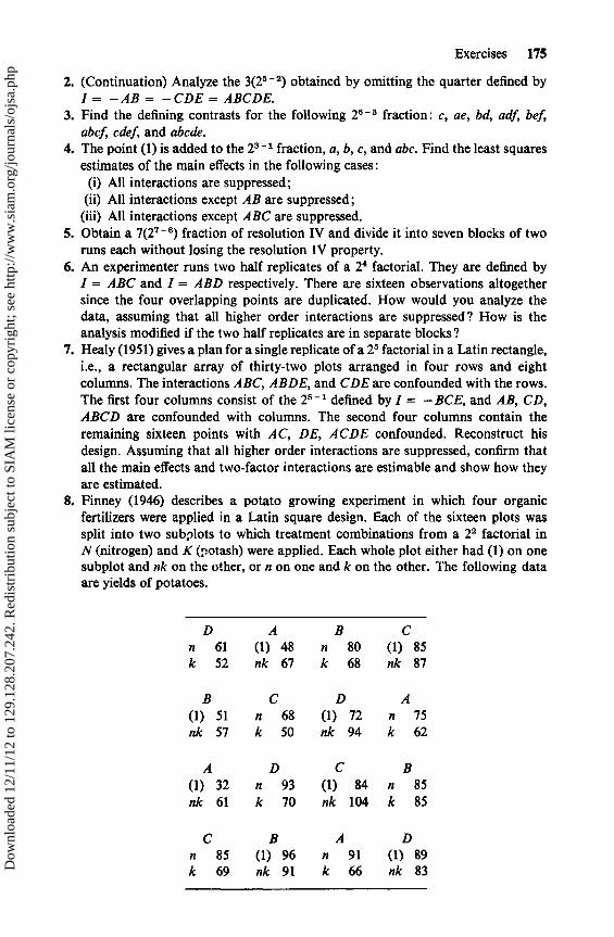
Exercises 175
2. (Continuation) Analyze the 3(25-1) obtained by omitting the quarter defined byI = — AB= — CDE = ABCDE.
3. Find the defining contrasts for the following 2 6-3 fraction: c, ae, bd, adf, bef,abcf, cdef, and abcde.
4. The point (1) is added to the 23-1 fraction, a, b, c, and abc. Find the least squaresestimates of the main effects in the following cases:(i) All interactions are suppressed;(ii) All interactions except AB are suppressed;
(iii) All interactions except ABC are suppressed.5. Obtain a 7(2 7 - e) fraction of resolution IV and divide it into seven blocks of two
runs each without losing the resolution IV property.6. An experimenter runs two half replicates of a 24 factorial. They are defined by
I = ABC and I = ABD respectively. There are sixteen observations altogethersince the four overlapping points are duplicated. How would you analyze thedata, assuming that all higher order interactions are suppressed? How is theanalysis modified if the two half replicates are in separate blocks?
7. Healy (1951) gives a plan for a single replicate of a 2 factorial in a Latin rectangle,i.e., a rectangular array of thirty-two plots arranged in four rows and eightcolumns. The interactions ABC, ABDE, and CDE are confounded with the rows.The first four columns consist of the 2 5 -1 defined by I = — BCE, and AB, CD,ABCD are confounded with columns. The second four columns contain theremaining sixteen points with AC, DE, ACDE confounded. Reconstruct hisdesign. Assuming that all higher order interactions are suppressed, confirm thatall the main effects and two-factor interactions are estimable and show how theyare estimated.
8. Finney (1946) describes a potato growing experiment in which four organicfertilizers were applied in a Latin square design. Each of the sixteen plots wassplit into two subplots to which treatment combinations from a 2 2 factorial inN (nitrogen) and K (potash) were applied. Each whole plot either had (1) on onesubplot and nk on the other, or n on one and k on the other. The following dataare yields of potatoes.
D A B Cn 61 (1) 48 n 80 (1) 85k 52 nk 67 k 68 nk 87
B C D A(1) 51 n 68 (1) 72 n 75nk 57 k 50 nk 94 k 62
A D C B(1) 32 n 93 (1) 84 n 85nk 61 k 70 nk 104 k 85
C B A Dn 85 (1) 96 n 91 (1) 89k 69 nk 91 k 66 nk 83D
ownl
oade
d 12
/11/
12 to
129
.128
.207
.242
. Red
istr
ibut
ion
subj
ect t
o SI
AM
lice
nse
or c
opyr
ight
; see
http
://w
ww
.sia
m.o
rg/jo
urna
ls/o
jsa.
php

176 Fractions of 2n Factorial Designs [Ch. 8
Analyze the data. Is it necessary to suppress the NK interaction? How would theanalysis be modified if A, B, C, and D were the four-treatment combinations in a22 factorial? How would it be modified if they were a 2 3 ' 1 of resolution III?Finney always confounded NK between whole plots. Could he perhaps haveconfounded the main effects N and K sometimes? Would he have gained anythingby it?
Dow
nloa
ded
12/1
1/12
to 1
29.1
28.2
07.2
42. R
edis
trib
utio
n su
bjec
t to
SIA
M li
cens
e or
cop
yrig
ht; s
ee h
ttp://
ww
w.s
iam
.org
/jour
nals
/ojs
a.ph
p

CHAPTER 9
FractionalFactorials
with MoreThan Two Levels
The fractions of the 2n designs that were discussed in the previous chapter areof considerable practical use as well as of academic interest. They enable us tohandle many factors without having to make an unreasonable number ofobservations, and it seems only natural that experimenters should wish to seekthe advantages of fractionation with factors having more than two levels. Newcomplications then arise; not only do factors at more than two levels call formore data points in the full design, but they also have more effects to bemeasured.
In a 2,1 experiment with all interactions involving three or more factorssuppressed, there are 1 + n + n(n — 1)/2 = (n2 + n + 2)/2 parameters to beestimated. In a 3' experiment each main effect has two degrees of freedom,corresponding to linear and quadratic effects; each two-factor interaction hasfour degrees of freedom, giving a total of 2n2 + 1 degrees of freedom. In a 5n
design the estimation of two-factor interactions soon gets out of hand; withonly three factors there are already 12 d.f. for main effects and forty-eight fortwo-factor interactions.
The interest in fractionation of 3n, 4n, and 5n designs is not merely for mathe-matical amusement. The model that was used for 2fz designs contained no termsin xh, and so, if the experimenter has cause to believe that for some factor there isa quadratic component to be estimated, he must take three or more levels. (Itwould be wrong to think that we always pay attention to estimating the quadraticcomponent, even when we suspect that it is there. In response-surface fitting,which will be discussed in the next chapter, we often elect to ignore the quadraticeffects in the earlier stages of experimentation and to make decisions aboutfuture experiments on the basis of first-order models.) The consideration ofcurvature thus leads us to 3n factorials, and we shall begin this chapter byrecalling some of the properties of 3" designs described in Chapter 7.
177
Dow
nloa
ded
12/1
1/12
to 1
29.1
28.2
07.2
42. R
edis
trib
utio
n su
bjec
t to
SIA
M li
cens
e or
cop
yrig
ht; s
ee h
ttp://
ww
w.s
iam
.org
/jour
nals
/ojs
a.ph
p
178 Fractional Factorials with More Than Two Levels [Ch. 9
We shall continue to use the concept of the resolution of a design that wasintroduced in the previous chapter. In view of the fact that the number of two-factor interactions increases so quickly with n, resolution V designs are of littleinterest and we shall not say much about them. The major use of these fractionalfactorials is in screening experiments, and so most of this chapter will be con-cerned with resolution III designs, which will often be called main effects plans.In the next section we shall recall the simplest of the main effects plans, theGraeco-Latin squares, and follow them with a discussion of 3n - ' factorials.
We shall then turn to the series of orthogonal resolution III designs, which areof considerable practical interest, developed by Plackett and Burman (1946) andby Addelman (1962). In that section we shall find some fractions of 2m3n designs,i.e., designs with m + n factors, of which m appear at two levels and the other nat three levels. The discussion of 2m3n designs will be developed further in latersections, and the chapter will conclude with a few examples of nonorthogonalfractions.
We have purposely restricted our discussion in this chapter to these topics.The reader who is particularly interested may wish to read some of the earlierpapers on the subject of fractionation of sn designs where s = pm and p is aprime. Among the papers of interest are some on orthogonal arrays. We note inparticular papers by Bose (1947a), Rao (1946) and (1947b), Bose and Bush(1952), and Finney (1945).
An orthogonal array (N, k, s, d) is a set of N treatment combinations with kfactors each at s levels, which has the property that for any subset of d out of thek factors all s' of the treatment combinations occur the same number of times;d is called the strength of the array. An orthogonal array of strength 2 is anorthogonal main effects plan. The levels of the factors will usually be denoted by0, 1, 2, ..., s — 1. If s is prime, these symbols will actually be elements of theGalois field GF(s). We shall sometimes write the levels of a two-level factorsymbolically as zero and one; this will be purely symbolic and they will betreated as the two elements of GF(2) with 1 + 1 = 0. In practice, the levels willstill be ± 1. The 2e - ' defined by I = — ABC may be written 000, 110, 101, and011. Consider the subset of factors A, B. We see that the set of treatmentcombinations 00, 01, 10, and 11 occurs once each. The same thing is true for thetreatment combinations of the subsets A, C and B, C. The design is thus anorthogonal array (4, 3, 2, 2).
9.1 3n Designs
The 3 2 and 3 3 experiments were discuseed in Chapter 7. At that time we tooka 3 2 example and divided the four degrees of freedom for A x B interaction intofour components: lin A lin B, lin A quad B, quad A lin B, and quad A quad B.We shall no longer use that method of subdivision of the interaction sum ofsquares because it does not lead to reasonable procedures for finding fractions.Instead we shall adopt a procedure used previously for confounding.
Dow
nloa
ded
12/1
1/12
to 1
29.1
28.2
07.2
42. R
edis
trib
utio
n su
bjec
t to
SIA
M li
cens
e or
cop
yrig
ht; s
ee h
ttp://
ww
w.s
iam
.org
/jour
nals
/ojs
a.ph
p

Sec. 9.2] Latin Squares as Main Effects Plans 179
The three levels of each factor are represented by 0, 1, and 2, and arithmetic iscarried out mod 3. The twenty-seven points of the 3 3 design form a finitegeometry in three-dimensional space. The sum of squares for A may be dividedinto two single degrees of freedom, corresponding to linear and quadraticeffects. The linear contrast is the difference between the sum of the observationsat xl = 2 and the sum at x l = 0, which we write as {x 1 = 2} — {x 1 = 0}. Thequadratic contrast is {x, = 0} — 2{x 1 = 1} + {x 1 = 2}. The equations x l = 0,x l = 1, and x l = 2 determine hyperplanes (in three dimensions they are justplanes). The degrees of freedom correspond to the two orthogonal contrastsbetween the totals of observations on the parallel planes.
For the A x B interaction we take the two sets of parallel planes xl + x2
0, 1, 2 (mod 3) and x l + 2x2 = 0, 1, 2 (mod 3). For each set of three planesthere are two orthogonal contrasts, and hence 2 degrees of freedom. We call thefirst pair of degrees of freedom the AB interaction and the second pair the AB 2
interaction. Nothing further is gained by considering the planes 2x 1 + x2
0, 1, 2 because the set of points with 2x 1 + x2 - c has 2(2x 1 + x2) - 2c, or,reducing mod 3, x l + 2x2 = 2c, and this again gives the AB2 interaction.
The three-factor interaction A x B x C has 8 degrees of freedom and fourcomponents, ABC, AB2C, ABC 2 , and AB'C 2, corresponding to sets of hyper-planes, x l + x2 + x3 - 0, 1, 2, x l + 2x2 + x3 - 0, 1, 2, x l + x2 + 2x3
0, 1, 2, and x l + 2x2 + 2x3 - 0, 1, 2, respectively. It is conventional to writethe components of interactions with the exponent of the first factor unity. Wegave an example of confounding the 33 factorial in three blocks of nine pointseach. Each of the blocks is a one-third replicate of the Pull factorial, which wemay write as a 33-1 fraction or, extending the notation that we introduced in thelast sections of the previous chapter, as a 3 1/ /9 design. Indeed, each of the blocksis a resolution III design, which leads us into the next section.
9.2 Latin Squares as Main Effects PlansWe originally presented the s x s Latin squares as designs for eliminating
plot differences in two directions: rows and columns. There is nothing in ourmodel or in the derivation of the analysis to prevent us from letting the rowsrepresent the s levels of one factor and the columns represent the s levels of asecond factor. Thus we see the Latin square of side s as an orthogonal maineffects plan for three factors, each at s levels in s2 runs. The Graeco-Latin squareis a main effects plan for four factors, and so on.
When we divided the 3 3 design into three blocks of nine points, the first blockconsisted of the points for which x l + 2x2 + 2x3 = 0. If we let x, denote therow and x 2 the column, this gives the Latin square
000 012 021
101 110 122
202 211 220.
Dow
nloa
ded
12/1
1/12
to 1
29.1
28.2
07.2
42. R
edis
trib
utio
n su
bjec
t to
SIA
M li
cens
e or
cop
yrig
ht; s
ee h
ttp://
ww
w.s
iam
.org
/jour
nals
/ojs
a.ph
p

180 Fractional Factorials with More Than Two Levels [Ch. 9
There are eight degrees of freedom in a 3 x 3 Latin square, and so there isroom for a fourth factor. We put x4 = xl + x2 and obtain a saturated maineffects plan or 34/ /9:
0000 0121 0212
1011 1102 1220
2022 2110 2201.
In the more general case, where s = pm, the s x s Latin square can be made toaccomodate s + 1 factors, each at s levels, in an orthogonal main effects plan.An interesting pioneering example of a 55-3, due to L. H. C. Tippett, is reportedby Fisher (1947). The factors involved were four different components of aspindle used in a cotton mill, each at five levels, and time, observations havingbeen made at five different periods.
The case s = 4 = 22 was also considered in Chapter 7. Here we have twopossible methods of attack. The finite geometry approach that we have adoptedso far implies the use of finite fields. In the case of s = 3 or 5, the elements ofthe field are the residue classes mod s. For s = 4 we can denote the levels of eachfactor by 0, 1, x, and y (= 1 + x) with arithmetic mod 2. When we blocked the42 experiment into four blocks of four, we took as the blocking factor C:x3 = yxl + yx2 . This also gives us a Latin square 4 3/ /16 main effects plan:
000 l0y x01 y0x
Oly 110 xlx yll
Oxl lxx xx0 yxy
Oyx lyl xyy yy0.
We also mentioned at that time the second method of attack, which involvesreplacing each four-level factor by two two-level factors.
The remarks that were made earlier about the bias resulting from interactionin Latin square designs are again relevant. In the last design A is aliased withB x C, B with A x C, and C with A x B.
In addition to the Graeco-Latin squares, there are other larger 3' - k fractionswhich are main effects plans. The principle of their constructiop is the same asthat for 2' - k designs of resolution III; we take a basic 3n design and add otherfactors by equating them to interactions, or rather to components of inter-actions. The following example will illustrate the procedure. We shall obtain atwenty-seven point resolution III 313-10 design and show how it becomes a39-6 in nine blocks of three points each.
Dow
nloa
ded
12/1
1/12
to 1
29.1
28.2
07.2
42. R
edis
trib
utio
n su
bjec
t to
SIA
M li
cens
e or
cop
yrig
ht; s
ee h
ttp://
ww
w.s
iam
.org
/jour
nals
/ojs
a.ph
p
Sec. 9.3] 3n -k Fractions with Interactions 181
We begin by taking a 3 3 design in the three factors A, B, and C and then addnew factors by setting
x4 = x1 + 2x3, x5 = 2X1 + x2 + x3, x6 = x2 + 2x3,
x7 = 2x 1 + x2 + 2x3 , x8 = x l + x2 + x3 , x9 = xl + x2,
X10 = Xl + X3, x11 = Xl + x2 + 2x3, x12 = xl + 2x2,
X13 = x2+ X3.
This is equivalent to taking as defining contrasts AC 2 D 2 , AB2 C 2E, BC 2F2 ,
AB2CG, ABCH 2 , ABJ 2, ACK 2, ABC 2L2 , AB2M2, and BCN 2 . The twenty-sevenpoints in the design follow:
0000000000000 0221100122011 0112200211022
1122221120000 1010021212011 1201121001022
2211112210000 2102212002011 2020012121022
1001202111110 1222002200121 1110102022102
2120120201110 2011220020121 2202020112102
0212011021110 0100111110121 0021211202102
2002101222220 2220201011201 2111001100212
0121022012220 0012122101201 0200222220212
1210210102220 1101010221201 1022110010212.
Suppose now that we decide to block the design by using the last two factors,M and N, as blocking factors, i.e., by assigning to the same block those pointsthat have the same value for x 12 and the same value for x 13 . There will be nineblocks corresponding to the pairs of coordinates 00, 01, 02, ..., and in thearrangement in which we have written the points they are the first three points,the middle three points, and the last three points of each column. There areeight degrees of freedom between blocks. Four of these are the 2 degrees offreedom each for M and N. The remaining 4 degrees of freedom are for thegeneralized interactions of M and N, namely K and L, which also becomeblocking factors since we have
X12 + X13 = xl + x3 = x10, x12 + 2x13 = xl + x2 + 2X3 = x11.
The blocked design is thus a resolution III 3 9-6 design in the first nine factors.
9.3 3n - k Fractions with Interactions
There is an extensive list of 3 fractions in the pamphlet prepared byConnor and Zelen (1959) for the National Bureau of Standards. In it theyconsider designs of resolution IV and resolution V with blocking for 4 < n < 10.
Dow
nloa
ded
12/1
1/12
to 1
29.1
28.2
07.2
42. R
edis
trib
utio
n su
bjec
t to
SIA
M li
cens
e or
cop
yrig
ht; s
ee h
ttp://
ww
w.s
iam
.org
/jour
nals
/ojs
a.ph
p
182 Fractional Factorials with More Than Two Levels [Ch. 9
The smallest resolution IV design for n = 4 is the one-third replicate, of whichan example will be given in the next section. For 5 < n < 9, they have resolutionIV designs with eighty-one points. Among the resolution V designs, eighty-onepoints are necessary for n = 4 or 5. For 6 < n < 9, resolution V designs arelisted with 243 points.
The 35/ /81 design can be obtained by using any of the five-factor interactionsas a defining contrast. The resolution IV 39/ /81 design is obtained by setting
x5 = x1 + 2x3 + x4, x6 = 2x1 + x2 + x3 + 2x4, x7 = x2 + 2x3 + x4,
x8 =2x1 +x2 +2x3 , x9 =x1 +x2 +x3 +x4 .
They obtain their 39/ /243 design by adding new factors to the basic 35 design asfollows :
x6 = xl + x2 + 2x3 + X5, X7= 2x1 + X2 + 2x4 + x5,
x8 = x2 + x3 + 2x4 + 2x5, x9 = xl + x2 + x3 + x4.
EXAMPLE OF A 34-1 DESIGN. Vance (1962) reports on a series of experi-ments in the course of which a 341 factorial was used. There were four majoroperating variables in the treatment of lube oil at a refinery, and these weretaken as the factors in the experiment. The objective of the experimentalprogram was to find a set of operating conditions that would optimize a measureof quality in the lube oil, which will be referred to as the response. Their previousexperience in the use of the plant had convinced Vance and his tolleagues thatthe quadratic effects should be estimated, and so at least three levels of eachfactor should be included.
In this preliminary experiment they were prepared to allow two-factor inter-actions to be aliased with each other. Their main concern was to obtain pre-liminary estimates of the linear and quadratic effects, aliased only by higherorder interactions, and to use this information to provide a basis for the designof subsequent experiments. This approach is similar to the procedure used infitting response surfaces, which will be discuseed in Chapter 10.
They had a choice of several possible fractions. In the 2 4 factorial there areonly two half replicates that have ABCD as the defining contrast. There are,however, no fewer than twenty-four 34-1 fractions in which the defining con-trast is some form of the four-factor interaction. We can take as the points of thefraction the set of points on any of the hyperplans defined by
xl + a2x2 + a3x3 + a4x4 = b (mod 3),
where a, = 1 or 2 and b = 0, 1, or 2.There is usually no particular reason for choosing any one of these fractions
over the others. Vance elected to use the fraction defined by
X1 + X2 + X3 + X4 = 0.
Dow
nloa
ded
12/1
1/12
to 1
29.1
28.2
07.2
42. R
edis
trib
utio
n su
bjec
t to
SIA
M li
cens
e or
cop
yrig
ht; s
ee h
ttp://
ww
w.s
iam
.org
/jour
nals
/ojs
a.ph
p
Sec. 9.3] 3"- k Fractions with Interactions 183
The experimental points and the reported responses are
0000 4.2 0012 5.9 0021 8.20102 13.1 0111 16.4 0120 30.70201 9.5 0210 22.2 0222 31.01002 7.7 1011 16.5 1020 14.31101 11.0 1110 29.0 1122 55.01200 8.5 1212 37.4 1221 66.32001 11.4 2010 21.1 2022 57.92100 13.5 2112 51.6 2121 76.52202 31.0 2211 74.5 2220 85.1.
We can now carry out the analysis of variance procedure for the basic 3 3
factorial in the usual way and obtain sums of squares for the main effectsA, B, C, and the interactions. These sums of squares are given in Table 9.1. Thesum of squares for D is calculated just as the sum of squares for the other maineffects, by adding the squares of the totals at the several levels of x 4 , dividing bynine, and subtracting the correction for the mean.
The two-factor interactions are hopelessly jumbled. If we work in terms of thesymbolic components of interaction we can untangle the web to a certainextent, but it is hardly worthwhile. Consider for example the A x D interaction,which has four degrees of freedom. The AD interaction involves contrastsbetween sums of points with x l + x4 - const (mod 3). Since we also have thedefining relationship x l + x2 + x3 + x4 = 0, it follows that for these points(x 1 + x2 + x3 + x4) + 2(x1 + x4) - const, i.e., x2 + x3 = const, and so theAD contrasts are also BC contrasts. Similarly, we have xl + 2x2 + 2x3 + x4
const, and so the AD contrasts are also AB2C 2D contrasts.An equivalent approach is to argue that the defining contrasts are I, ABCD,
A 2B2 C 2D2. Multiplying by AD and letting A 3 = B3 = C 3 = D3 = I gives analias set AD, A 2BCD2, B2 C 2 . Finally, squaring the last two members to makethe exponent of the first letter unity gives the set AD, AB2C 2D, BC. We canproceed in this way to obtain the aliases of each component (2 d.f.) in the 3 3
experiment. If we ignore interactions involving three or more factors, the aliassets are
A; B; C; AB, CD; AB2 ; AC, BD; AC 2 ; BC, AD;
BC 2 ; (ABC), D; (AB2C), BD2 ; (ABC 2), CD2 ; (AB2C 2), AD2 .
The crucial difference between this and the 2 4 -1 fractional factorial defined byI = ABCD is that in the Jatter the A x D interaction is completely aliased, orconfounded, with the B x C interaction. In the present case two of the degrees offreedom of the A x D interaction are aliased with BC, and the other twodegrees of freedom come from the A x B x C interaction sum of squares. A
Dow
nloa
ded
12/1
1/12
to 1
29.1
28.2
07.2
42. R
edis
trib
utio
n su
bjec
t to
SIA
M li
cens
e or
cop
yrig
ht; s
ee h
ttp://
ww
w.s
iam
.org
/jour
nals
/ojs
a.ph
p

184 Fractional Factorials with More Than Two Levels [Ch. 9
more meaningful aliasing would have been one where, for example, lin A x lin Bwas aliased with quad C x quad D, but we cannot obtain such relationshipsusing this method of obtaining fractions.
TABLE 9.1
ANALYSIS OF VARIANCE
Source SS d.f.
Total 15544.5 26A 4496.3 2(lin A 4399.2 1)(quad A 97.1 1)B 2768.7 2(lin B 2647.5 1)(quad B 121.2 1)C 5519.8 2(lin C 5516.0 1)(quad C 3.8 1)D 283.4 2(lin D 213.6 1)(quad D 69.8 1)(Total for main effects 13068.2 8)A x B 310.8 4AxC 1232.9 4B x C 669.8 4A x B x C (excluding D) 262.8 6
9.4 Orthogonal Main Effects Plans
We have already discussed saturated 2' -' and 3n - k fractions, in which thebasic design is "loaded" with additional factors by equating them to inter-actions. This procedure has given us orthogonal main effects plans for 2n — 1two-level factors in 2n runs and for (3n — 1)/2 three-level factors in 3n runs.Plackett and Burman (1946) discovered a series of orthogonal saturated resolu-tion III designs for N — 1 factors in N runs when N = 4k where k is an integer.Their designs were mentioned in passing in Chapter 8, and a discussion of themhas been postponed until now. They listed designs for all values of N = 4k up toN = 100, with the exception of N = 92. The case N = 92 was solved byBaumert, Golomb, and Hall (1962). The other major contribution to orthogonalmain effects plans to be discussed at this time is due to Addelman (1962), whoshowed how new plans could be obtained by collapsing and replacing factors inthe basic series of designs by other factors which have different numbers oflevels.
Dow
nloa
ded
12/1
1/12
to 1
29.1
28.2
07.2
42. R
edis
trib
utio
n su
bjec
t to
SIA
M li
cens
e or
cop
yrig
ht; s
ee h
ttp://
ww
w.s
iam
.org
/jour
nals
/ojs
a.ph
p

Sec. 9.5] The Plackett and Burman Designs 185
9.5 The Plackett and Burman Designs
These are designs for factors at two levels which we denote by + and —,standing for x i = + 1 and x t = —1, respectively. Let X denote the designmatrix. If there are N points and n factors, X is a matrix with N rows and ncolumns in which x h{ is the value (+ or —) of x i at the hth point. We have themain effects model
E(y) _ Po + Psxnil
or E(Y) = D13 where D = (1, X) and 13' = Po, P1, P2, ..., Pn.We wish to find a design such that the matrix D'D is diagonal. Since
xki = 1 for all h and all i, the diagonal elements of D'D are each equal to N,and so we require D'D = NI, i.e., that the column vectors of X be orthogonalto each other and to 1.
We denote by X { the ith column of X, consisting of the values taken by x ti ateach design point. If 1'X i = c{, Margolin (1967) defines X i to be a columnvector of value c i . If ci = 0, X{ is called a zero-sum column vector. lf c i 0, X i iscalled a nonzero-sum column vector. If D'D is to be diagonal, each X, mustbe a zero-sum column vector, which means that half the entries must be plusand half minus. Similarly, if we let (X i , X;) denote the inner product X,Aj , weneed to have (Xi , X;) = 0 for all pairs i, j(i ^ j). If n = N — 1, which is thelargest number of factors at two levels that we can hope to accommodate, theproblem of finding a suitable design becomes one of finding a matrix D of Nrows and N columns with the following properties:
(i) Each element is ± 1;(ii) One column of D is 1;(iii) N -112D is orthogonal. Such a matrix is called a Hademard matrix.
We shall now show how Plackett and Burman obtained their designs. Thereader who does not wish to follow the derivation, which involves the use offinite fields, can safely skip to the end of this section, where we list the designfor N = 12. This method of constructing a Hademard matrix is due to Paley(1933).
Let z be any nonzero element of the finite field GF(pm); z is said to be aquadratic residue of the field if there is an element w in the field such thatw2 = z; otherwise, z is a nonquadratic residue. If p >_ 3, it can be shown thatthe number of nonzero elements that are quadratic residues is equal to thenumber that are nonquadratic residues. We introduce the Legendre symbol, x(z),defined as follows (it will be used in a slightly different fashion in Chapter 13):
x(0) = 0 ;
x(z) = + 1, if z is a quadratic residue;
x(z) = —1, if z is a nonquadratic residue.
Dow
nloa
ded
12/1
1/12
to 1
29.1
28.2
07.2
42. R
edis
trib
utio
n su
bjec
t to
SIA
M li
cens
e or
cop
yrig
ht; s
ee h
ttp://
ww
w.s
iam
.org
/jour
nals
/ojs
a.ph
p

186 Fractional Factorials with More Than Two Levels [Ch. 9
It follows that 1 x(z) = 0, summing over all z in GF(pm). Three other resultsabout the Legendre symbols are needed, and we state them without proof.
(i) Let z' be another element of GF(pm). Then X(z)X(í) = x(zí ), in particularx(- z) = x(- 1 )x(z);
(ii) x( -1) = +1, ifpm = 4k + 1, x( -1) _ —1, ifpm = 4k — 1 where k is aninteger;
(iii) Let u and v be two elements of the field u 0 v, p > 2. Then, summing overall zin the field x(z — u)x(z — v) = —1.
Using these results, we can construct a Hademard matrix of order N whereN = pm + 1 = 4k.
We number the rows and columns of a matrix X, h, and 1 where h and i areelements of GF(pm), and add one extra row, which has every element minus;X is a matrix of pm + 1 rows and pm columns. The elements of the first pm rowsare assigned as xhh = + 1, xhi = — X(h — i) (h 0 i).
Consider the matrix D = (1, X). For this matrix we have
1'X{ =-1 + 1 —1X(h—i)=0,h
(X1, Xi) = 1 — x(i — j) — X(j — i) + x(h — i)x(h — j)h
= 1 —x(i— j)—x(J—i)— 1.
But with pm = 4k — 1 we have x(j — i) = x(-1)x(i — j) = —x(i — j), so that(Xi , X1) = 0. The matrix D is thus a Hademard matrix.
We also note that if D is any Hademard matrix of order N,
D* _ (D DD D)
is a Hademard matrix of order 2N, and so a design for 2N — 1 factors in 2Nruns can be constructed from a design for N — 1 factors in N runs.
If pm = 4k + 1, Plackett and Burman show that the foregoing constructionprocedure can be modified to obtain a Hademard matrix of order 2(pm + 1),and the reader is referred to their paper for the details. They used this method toobtain designs for N = 52, 76, and 100. Their design for N = 36 was obtainedby trial.
It should also be noted that if N = p + 1, i.e., m = 1, then, apart from thelast row which represents the base point (1), X is a circulant matrix. We have
= x,, and so in their listing the authors give only one line of eachmatrix for those values of N.
As an example we now derive the Plackett and Burman design for N = 12,p = 11. The elements of GF(1 1) are 0, 1, 2,..., 10 with arithmetic being carriedout mod 11. The quadratic residues are 1 = 1 2 = 102 , 4 = 22 = 92 , 9 = 32 =
Dow
nloa
ded
12/1
1/12
to 1
29.1
28.2
07.2
42. R
edis
trib
utio
n su
bjec
t to
SIA
M li
cens
e or
cop
yrig
ht; s
ee h
ttp://
ww
w.s
iam
.org
/jour
nals
/ojs
a.ph
p
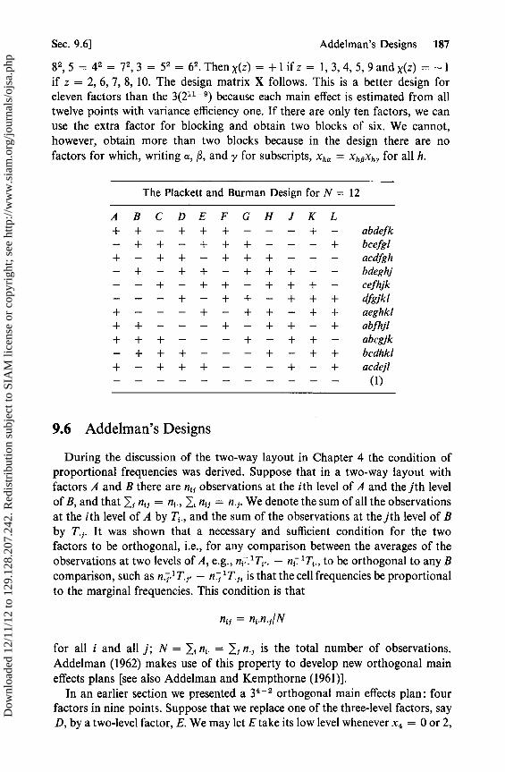
Sec. 9.6] Addelman's Designs 187
8 2 , 5 = 42 = 7 2 , 3 = 5 2 = 62 . Then X(z) = + 1 if z = 1, 3, 4, 5, 9 and X(z) = —1if z = 2, 6, 7, 8, 10. The design matrix X follows. This is a better design foreleven factors than the 3(211-9) because each main effect is estimated from alltwelve points with variance efficiency one. If there are only ten factors, we canuse the extra factor for blocking and obtain two blocks of six. We cannot,however, obtain more than two blocks because in the design there are nofactors for which, writing a, P, and y for subscripts, x, = xh$xhy for all h.
The Plackett and Burman Design for N = 12
A B C D E F G H J K L+ + — + + + — — — + — abdefk— + + — + + + — — — + bcefgl+ — + + — + + + — — — acdfgh— + — + + — + + + — — bdeghj— — + — + + — + + + — cefhjk— — — + — + + — + + + dfgjkl+ — — — + — + + — + + aeghkl+ + — — — + — + + — + abfhjl+ + + — — — + — + + — abcgjk— + + + — — — + — + + bcdhkl+ — + + + — — — + — + acdejl— — — — — — — — — — — (1)
9.6 Addelman's Designs
During the discussion of the two-way layout in Chapter 4 the condition ofproportional frequencies was derived. Suppose that in a two-way layout withfactors A and B there are n11 observations at the ith level of A and the jth levelof B, and that Ij n t1 = n { ., l i ntj = n. j . We denote the sum of all the observationsat the ith level of A by Ti ., and the sum of the observations at thejth level of Bby T. ;. It was shown that a necessary and sufficient condition for the twofactors to be orthogonal, i.e., for any comparison between the averages of theobservations at two levels of A, e.g., n ;-.'Ti .. — n 1.., to be orthogonal to any Bcomparison, such as n.-J- 1 T 1- — n.. i 'T 1, is that the cell frequencies be proportionalto the marginal frequencies. This condition is that
nif = n{ .n. f/N
for all i and all j; N = I, n i. = If n. ; is the total number of observations.Addelman (1962) makes use of this property to develop new orthogonal maineffects plans [see allo Addelman and Kempthorne (1961)].
In an earlier section we presented a 34_2 orthogonal main effects plan: fourfactors in nine points. Suppose that we replace one of the three-level factors, sayD, by a two-level factor, E. We may let E take its low level whenever x4 = 0 or 2,
Dow
nloa
ded
12/1
1/12
to 1
29.1
28.2
07.2
42. R
edis
trib
utio
n su
bjec
t to
SIA
M li
cens
e or
cop
yrig
ht; s
ee h
ttp://
ww
w.s
iam
.org
/jour
nals
/ojs
a.ph
p
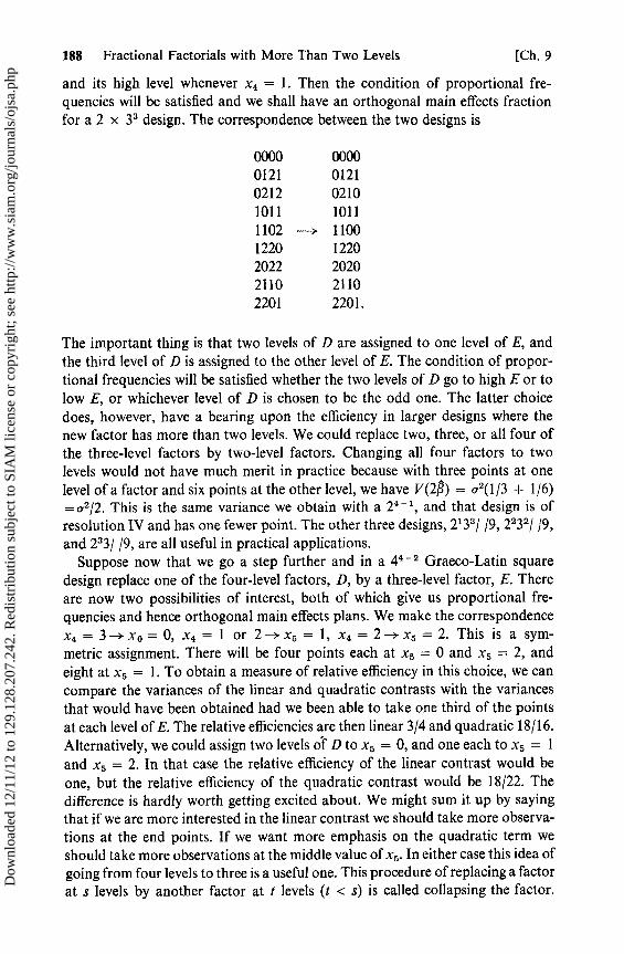
188 Fractional Factorials with More Than Two Levels [Ch. 9
and its high level whenever x 4 = 1. Then the condition of proportional fre-quencies will be satisfied and we shall have an orthogonal main effects fractionfora 2 x 33 design. The correspondence between the two designs is
0000 00000121 01210212 0210
1011 10111102 --> 11001220 12202022 2020
2110 2110
2201 2201.
The important thing is that two levels of D are assigned to one level of E, andthe third level of D is assigned to the other level of E. The condition of propor-tional frequencies will be satisfied whether the two levels of D go to high E or tolow E, or whichever level of D is chosen to be the odd one. The latter choicedoes, however, have a bearing upon the efficiency in larger designs where thenew factor has more than two levels. We could replace two, three, or all four ofthe three-level factors by two-level factors. Changing all four factors to twolevels would not have much merit in practice because with three points at onelevel of a factor and six points at the other level, we have V(21) = a 2(1/3 + 1/6)= a2/2. This is the same variance we obtain with a 2 -1 , and that design is ofresolution IV and has one fewer point. The other three designs, 2'3 3/ /9, 2232/ /9,and 233/ /9, are all useful in practical applications.
Suppose now that we go a step further and in a 44 - 2 Graeco-Latin squaredesign replace one of the four-level factors, D, by a three-level factor, E. Thereare now two possibilities of interest, both of which give us proportional fre-quencies and hence orthogonal main effects plans. We make the correspondencex4 = 3 —^ x o = 0, x4 = 1 or 2—x5x5 = 1, x4 = 2 —^ x5 = 2. This is a sym-metric assignment. There will be four points each at x 5 = 0 and x5 = 2, andeight at x5 = 1. To obtain a measure of relative efficiency in this choice, we cancompare the variances of the linear and quadratic contrasts with the variancesthat would have been obtained had we been able to take one third of the pointsat each level of E. The relative efficiencies are then linear 3/4 and quadratic 18/16.Alternatively, we could assign two levels of D to x5 = 0, and one each to x5 = 1and x5 = 2. In that case the relative efficiency of the linear contrast would beone, but the relative efficiency of the quadratic contrast would be 18/22. Thedifference is hardly worth getting excited about. We might sum it up by sayingthat if we are more interested in the linear contrast we should take more observa-tions at the end points. If we want more emphasis on the quadratic term weshould take more observations at the middle value of x 5 . In either case this idea ofgoing from four levels to three is a useful one. This procedure of replacing a factorat s levels by another factor at t levels (t < s) is called collapsing the factor.
Dow
nloa
ded
12/1
1/12
to 1
29.1
28.2
07.2
42. R
edis
trib
utio
n su
bjec
t to
SIA
M li
cens
e or
cop
yrig
ht; s
ee h
ttp://
ww
w.s
iam
.org
/jour
nals
/ojs
a.ph
p
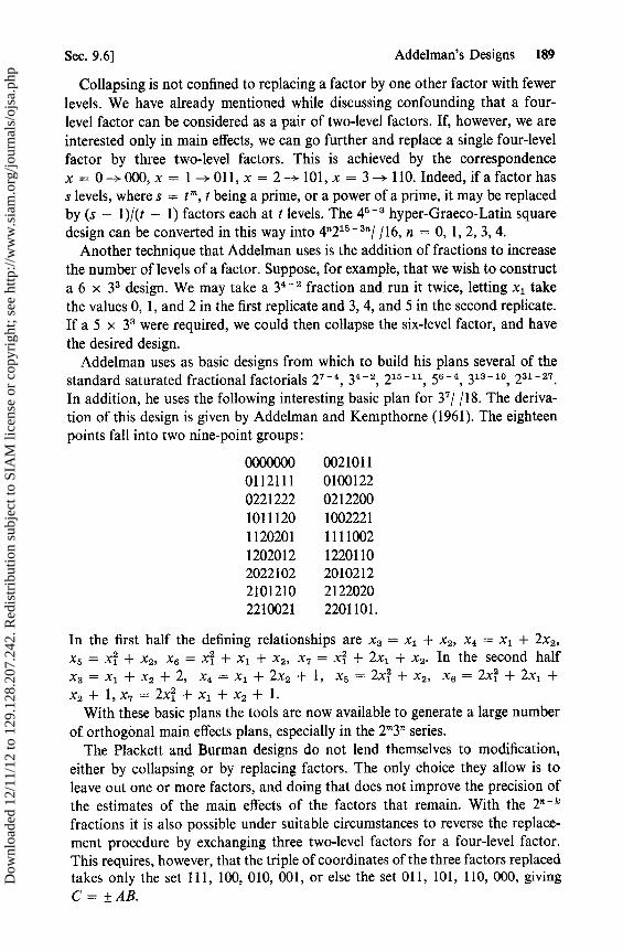
Sec. 9.6] Addelman's Designs 189
Collapsing is not confined to replacing a factor by one other factor with fewerlevels. We have already mentioned while discussing confounding that a fourlevel factor can be considered as a pair of two-level factors. If, however, we areinterested only in main effects, we can go further and replace a single four-levelfactor by three two-level factors. This is achieved by the correspondencex = 0 -+ 000, x = 1 -+ 011, x = 2 -+ 101, x = 3 -+ 110. Indeed, if a factor hass levels, where s = t'", t being a prime, or a power of a prime, it may be replacedby (s - 1)/(t - 1) factors each at t levels. The 45 - 3 hyper-Graeco-Latin squaredesign can be converted in this way into 4n2l5-3n/ /16, n = 0, 1,2,3,4.
Another technique that Addelman uses is the addition of fractions to increasethe number of levels of a factor. Suppose, for example, that we wish to constructa 6 x 33 design. We may take a 34
-2 fraction and run it twice, letting Xl take
the values 0, 1, and 2 in the first replicate and 3, 4, and 5 in the second replicate.If a 5 x 33 were required, we could then collapse the six-level factor, and havethe desired design.
Addelman uses as basic designs from which to build his plans several of thestandard saturated fractional factorials 27-\ 34 - 2, 215- 11, 56 - \ 313-1°,231-27.In addition, he uses the following interesting basic plan for 37 / /18. The derivation of this design is given by Addelman and Kempthorne (1961). The eighteenpoints fall into two nine-point groups:
00000oo01121110221222101112011202011202012202210221012102210021
002101101001220212200100222111110021220110201021221220202201101.
In the first half the defining relationships are X3 = Xl + X 2, X4 = Xl + 2X2'
X5 = xi + X2, X6 = xi + Xl + X 2, X7 = xi + 2Xl + X2' In the second halfX3 = Xl + X2 + 2, X4 = Xl + 2X2 + 1, X5 = 2xi + X 2, X 6 = 2xi + 2Xl +X2 + I, X7 = 2xi + Xl + X2 + 1.
With these basic plans the tools are now available to generate a large numberof orthogonal main effects plans, especially in the 2m3n series.
The Plackett and Burman designs do not lend themselves to modification,either by collapsing or by replacing factors. The only choice they allow is toleave out one or more factors, and doing that does not improve the precision ofthe estimates of the main effects of the factors that remain. With the 2n - k
fractions it is also possible under suitable circumstances to reverse the replacement procedure by exchanging three two-level factors for a four-level factor.This requires, however, that the triple of coordinates of the three factors replacedtakes only the set 111, 100, 010, 00I, or else the set 011, 101, 110, 000, givingC = ±AB.
Dow
nloa
ded
12/1
1/12
to 1
29.1
28.2
07.2
42. R
edis
trib
utio
n su
bjec
t to
SIA
M li
cens
e or
cop
yrig
ht; s
ee h
ttp://
ww
w.s
iam
.org
/jour
nals
/ojs
a.ph
p

190 Fractional Factorials with More Than Two Levels [Ch. 9
Consider changing the 2' - 4 design, (1), adef, befg, abdg, cdeg, acfg, bcdf, abceinto a 3 x 2 orthogonal main effects plan. The generators of the definingcontrast subgroups are 1, —ACD, ABCE, —ABF, —BCG. At each pointxl + x 3 + x4 - 0 (mod 2). We can therefore replace A, C, and D by a four-level factor, letting 000 —* 0, 011 -> 1, 101 2, 110 3. We then introducé thethree-level factor by collapsing the four-level factor that we have just acquired;we collapse levels 2 and 3 to x 8 = 2. The final design follows, together with theoriginal eight points:
BEFGH
(1) 00000
adef 01102
befg 11110
abdg 10012
cdeg 01011
acfg 00112
bcdf 10101
abce 11002.
9.7 Fractions of 2m3n Designs of Resolution V
A listing of fractions of 2m3 7 designs was prepared by Connor and Young(1961) in the National Bureau of Standards series. More recently Margolin(1967) has investigated such fractions. In this section we shall give a briefsketch of Margolin's results. We shall use A to denote a factor with two levelsand R, S, T, U to denote factors with three levels. When we talk of a resolutionV design in this context we shall mean a design in which all such interactions asARL, ARQ , RLSL , RQSL, RL,SQ, RQ SQ are estimable. Interactions with three ormore factors will be suppressed.
In a complete 3m factorial the linear contrast for R is given by {R = 2} —{R = 0}, i.e., by the difference between the totals at the highest level of R andthe lowest level of R. The RLSL contrast is {R = 2, S = 2} + {R = 0, S = 0} —{R = 0, S = 2} — {R = 2, S = 0}. (This is not the kind of contrast betweenhyperplanes that we considered earlier.) In a 3n -p fraction of resolution IV themain effects will be clear, but there will be some linear dependencies between theinteraction terms. As an example, Margolin points out that if we take the 34-1fraction defined by x, + x, + xt + x„ = 1 (mod 3), there is a linear dependencybetween RLSL, RQSQ , TL and T0 U0 . Suppose now that we collapse the factorU into a two-level factor A by letting xu = 0, x,, = 2 x,, = 0, and x,, = 1 -^xa = 1. Then the linear U contrast and the interactions involving UL disappear.Contrasts involving levels of A correspond to UQ . The disappearance of UL
removes the dependency between the other three interactions. The ATe inter-action, for example, corresponds to the former T0U0.
Dow
nloa
ded
12/1
1/12
to 1
29.1
28.2
07.2
42. R
edis
trib
utio
n su
bjec
t to
SIA
M li
cens
e or
cop
yrig
ht; s
ee h
ttp://
ww
w.s
iam
.org
/jour
nals
/ojs
a.ph
p

Sec. 9.8] Two Nonorthogonal Fractions of the 4 3 Design 191
Using this idea Margolin obtains several fractions of 2m3n designs by collaps-ing factors in resolution IV 3n - P designs. The example that we have just men-tioned is a design of resolution V for 2 1 33/ /27. Collapsing a second factor wouldgive 223 2/ /27. He also gives a 22 34/ /81 fraction.
A second method of obtaining fractions is to run different 3n - p fractions ateach level of a two-level factor. An obvious example of a 2 1 35/ /2 1 3 4 would be torun a resolution V 3 5 -1 fraction at low A and another 35_1 (or the same one) athigh A. Similarly, a 253'/ /96 fraction may be formed by running one of theresolution V 2 5 -1 fractions at each level of the three-level factor. Margolin givestwo designs formed in this way. A 243'/ /24 design for four factors A, B, C, andD at two levels each and E at three levels is obtained by running the half replicatedefined by I = —ABCD at x5 = 0 and x5 = 1 and running the half replicatedefined by I = +ABCD at x5 = 2.
9.8 Two Nonorthogonal Fractions of the 4 3 Design
We mentioned earlier that a four-level factor may be replaced by a pair oftwo-level factors. The 4 3 factorial with factors P, Q, and R can thus be con-sidered as a 26 factorial where A and B correspond to P, C and D to Q, and Eand F to R. The three degrees of freedom for the main effect of P correspond toA, B, and AB. The nine degrees of freedom for PQ correspond to AC, AD,ACD, BC, BD, BCD, ABC, ABD, and ABCD.
The first fraction that we shall consider is a main effects only plan with twelvepoints. This will be a 3(2 6 - 4) fraction with all six main effects and the inter-actions AB, CD, and EF estimable. All other interactions are suppressed.Consider the family of 2 4 - 2 fractions of the factorial in A, B, C, and D definedby I = ± AD = ± BC = ± ABCD and add new factors by putting E = + ACD,F = +ABC. The four quarters are
(1), adf, bce, abcdef;cef, acde, bf, abd;de, aef, bcd, abcf;
cdf, ac, bdef, abe.
Any three of them constitute a 3(26_4) fraction for which the alias sets areI, AD, BC, ABCD; C, ACD(=E), B, ABD; D, A, BCD, ABC(=F); CD, AC,BD(=EF), AB. This is a main effects only plan. Furthermore, because thedefining contrasts AD, BC, and ABCD are all suppressed, the design may berun in three blocks of four runs each, the blocks being the three "quarters"chosen.
This design is actually a three-quarter fraction of the Latin square. Supposethat we let columns correspond to the levels (1), a, b, ab of P and rows to thelevels (1), c, d, cd of Q, and that we denote the levels (1), e, f, and ef of R by0, 1, 2, and 3, respectively. Furthermore, let us denote points in the four
Dow
nloa
ded
12/1
1/12
to 1
29.1
28.2
07.2
42. R
edis
trib
utio
n su
bjec
t to
SIA
M li
cens
e or
cop
yrig
ht; s
ee h
ttp://
ww
w.s
iam
.org
/jour
nals
/ojs
a.ph
p

192 Fractional Factorials with More Than Two Levels [Ch. 9
"quarters" by a, P, y, 8, respectively. When this is done we have a Graeco-Latinsquare:
(1) aef bf abe Oa 3y 2fl 18
cef ac bce abcf 3fl 08 la 2yde adf bdef abd ly 2a 38 0pcdf acde bed abcdef 28 1 fl Oy 3a.
Thus our design actually amounts to using the fourth factor (Greek letters) asa blocking factor and taking any three of the four blocks.
The second design is a resolution V fraction with forty-eight points. Thisdesign is the 3(28-2) fraction defined by I = ACE = BDF = ABCDEF. Thealias sets follow. The effects that correspond to degrees of freedom in theP x Q x R interaction, and are therefore suppressed, have been underlined.This design may be run in three blocks of sixteen runs each. An example is givenby John (1970).
I, ACE, BDF, ABCDEF ; A, CE, ABDF, BCDEF ;
B,ABCE, DF, ACDEF ; AB, BCE, ADF, CDEF;
C,AE, BCDF, ABDEF; AC, E, ABCDF, BDEF;
BC, ABE, CDF, ADEF; ABC, BE, ACDF, DEF;
D, ACDE, BF, ABCEF ; AD, CDE, ABF, BCEF ;
BD, ABCDE, F, ACEF; ABD, BCDE, AF, CEF;
CD, ADE, BCF, ABEF; ACD, DE, ABCF, BEF;
BCD, ARDE, CF, AEF; ABCD, BDE, ACF, EF.
Dow
nloa
ded
12/1
1/12
to 1
29.1
28.2
07.2
42. R
edis
trib
utio
n su
bjec
t to
SIA
M li
cens
e or
cop
yrig
ht; s
ee h
ttp://
ww
w.s
iam
.org
/jour
nals
/ojs
a.ph
p

CHAPTER 10
ResponseSurfaces
Most of the experimental designs that have been considered so far have hadtheir origins in agricultural experimentation. The development of 2n - k fractionalfactorials has taken place in industrial experimentation, but they were introducedin an agricultural context by Finney (1945). The concept of response surfaces anddesigns for their exploration began in the chemical industry. The early work wasdone by statisticians and chemical engineers in the Imperial Chemicals Industriesin Great Britain. The first major paper in the field was published by Box andWilson (1951). Its title, "On the Experimental Attainment of Optimum Condi-tions," is indicative of its philosophy.
Suppose for simplicity that we wish to investigate the production of lomechemical product in a pilot plant, and that there are two factors, temperatureand pressure, that are to be considered. The experimental procedure will be tomake several runs on the pilot plant at different temperatures and pressures andto observe on each run a response, y, such as the yield of the product, or thepurity of the product, or the amount of raw material converted, and so on.We have a two-dimensional factor space with two quantitative factors. We canconceive, therefore, of the expected response E(y) as a function of the levels ofthe factors. If xl denotes the temperature and x 2 the pressure we have
Y = ff(xj, x2) + e,
with the usual assumptions about the random error e. The function f(x 1 , x2) issingle valued and, writing 77 for E(y), the surface represented by 17 = f(x 1 , x2) iscalled the response surface. If the x l and x2 axes are taken in the usual wayand the y axis is taken perpendicular to the plan of the paper, the response
193
Dow
nloa
ded
12/1
1/12
to 1
29.1
28.2
07.2
42. R
edis
trib
utio
n su
bjec
t to
SIA
M li
cens
e or
cop
yrig
ht; s
ee h
ttp://
ww
w.s
iam
.org
/jour
nals
/ojs
a.ph
p
194 Response Surfaces [Ch. 10
surface can be represented on the paper, just as altitude is represented on a map,by drawing the lines of equal response as contours.
It may be that prior knowledge of the chemical process involved will enableus to know beforehand the form of f(x 1 , x2). The discussion of such models isoutside the scope of this book. We shall consider the situation in whichf(x1 , x2) is approximated by a polynomial of degree d, in which case the model iscalled a dth-order model. The set of points (x 1 , x2) at which runs can be made iscalled the factor space.
One possibility would be for us to take several levels of temperature andseveral levels of pressure to straddle the factor space, carry out a complete, orfractional, factorial experiment, and fit the model to the data as we have done inearlier chapters. This ignores three important features of this kind of experiment.
1. The usual object of the experiment is not to investigate f(x1 , x2) over thewhole factor space but to locate the region in the factor space where the responseis at its highest and to map it. If we regard the response surface as a mountain,the object is to find the peak and to explore the area in which the peak is found.The industrialist is rarely interested in regions where the yield of his process willbe relatively low.
2. A polynomial model will usually be quite unrealistic over the whole space,but its use in a relatively small region around the peak is acceptable as a Taylorseries expansion approximating a more complicated function.
3. Experimental runs on pilot plants, or actual commercial reactors, usuallyhave relatively high precision and can be conducted sequentially.
Our problem can thus be summarized: How do we find the region of thefactor space that interests us and, having found it, how do we design experimentsto map f(x 1 , x2) over that region? We shall discuss the second question first.
The remainder of the chapter can be divided into two areas: the design andanalysis of experiments for fitting first- and second-order models, and themethod of steepest ascent and EVOP.
The two most important papers on the topic of response surfaces are the oneby Box and Wilson (1951) mentioned before, and the paper by Box and J. S.Hunter (1957). Box and a group of workers at Imperial Chemical Industriesprepared a book, Design and Analysis of Industrial Experiments, edited byDavies (1954). The chapter on the determination of optimum conditionscontains several examples and is an excellent practical exposition. The readerwho wishes to pursue this subject further will find numerous references in the re-view paper on response surface methodology by Hill and W. G. Hunter (1966).
10.1 First-Order Designs
These are designs for fitting a first-degree equation:
y=Po +1Pix, +ei, i= 1,2,...,k.
Dow
nloa
ded
12/1
1/12
to 1
29.1
28.2
07.2
42. R
edis
trib
utio
n su
bjec
t to
SIA
M li
cens
e or
cop
yrig
ht; s
ee h
ttp://
ww
w.s
iam
.org
/jour
nals
/ojs
a.ph
p

Sec. 10.1] First-Order Designs 195
A simple example of such a design is the main effects only 2' - k fractionalfactorial where the coordinates of x j take the values ± 1. Before consideringoptimal designs it should be recalled that the coefficients S, are affected by thechoice of the scale of x { . If x1 denotes the length of some physical componentmeasured in feet, we can triple the value of J by measuring x, in units of yardsinstead. It is desirable, therefore, to scale the factors uniformly, and we shall dothis by imposing the, following restrictions upon the coordinates x, where xj' isthe value of xj at the jth experimental point:
x1 = 0, x41 = b,r r
where b is a constant. The first of these requirements is a shift in the origin so thatx, = 0 for all i; the second amounts to a change of scale to provide uniformscatter among the x,.
Let X denote the design matrix (xf,). The normal equations may be written
() Y = S,X
where
S = (1, X)'(1, X)= [0
and F3' = (Po, P1, ..., Pk). In comparing designs we shall take as a criterion theaverage variance of the regression coefficients, or
v = (k + 1 ) - 1{V($o) + > V(i )} = (k + 1) -1 tr(S -1).t J
For an optimal design we seek, therefore, to minimize
k
tr(S 1) _ Ah 1 ,h =0
where Xh are the latent roots of S and Ao = N. The trace is minimized subject to
the condition l Ah = tr S = N + kb or h = kb, in which case,
Ah =b
for all h where h = 1, 2, ..., k. This requires that S be a diagonal matrix, or,equivalently, that the columns of X be mutually orthogonal. This condition forX is both necessary and sufficient for a design to be optimal and for such adesign we have v($t) = b - laa, i > 0.
Some examples of optimal designs are the 2n - ' fractions and the Plackett andBurman designs for n factors. For k = 3 we can use the vertices of the regular
Dow
nloa
ded
12/1
1/12
to 1
29.1
28.2
07.2
42. R
edis
trib
utio
n su
bjec
t to
SIA
M li
cens
e or
cop
yrig
ht; s
ee h
ttp://
ww
w.s
iam
.org
/jour
nals
/ojs
a.ph
p

196 Response Surfaces [Ch. 10
tetrahedron with the center at the origin and any orientation. Also, for k = 2the vertices of the regular polygon inscribed in a circle with the center at theorigin form an optimal design.
10.2 Second-Order Designs
These are designs for fitting the second-degree surface (for k = 3, the generalquadric surface) :
E(Y1) = R0 + ,8x5 + + Nhixihxlt•t t h t
h<t
It is convenient to write the elements of E3 in the order
p , = (PO, P11, P22, • • • , Pkk, P19 P2, . • • 3 Pk, P12, .. • )•
Writing the normai equations as TY = Sp, we have
(TY)' _ Y^ x1Y^ ...91 x1Y, ..., > x1x2Y,....
We shall confine our investigation to designs that satisfy conditions ofsymmetry and scaling, which are similar to those for first-order designs. Thefollowing conditions, with h i, are imposed upon the set of points in thedesign:
xph = xih = xlhxlt — x'hX = x hXji = 0,i 1 i i
2 22 4^ xlnxlt = c, x1i = c + d.
The matrix S now takes a convenient form. In its top left-hand corner is theprincipal minor, U, with (k + 1) rows and columns which will now be dis-cussed. The remaining rows and columns consist of zero elements everywhereexcept on the main diagonal. The diagonal element corresponding to P i is b,so that P = x1iy1/b and V(Pt) = a2/b. Similarly, /hi = 1 xlhxliyi/c andv(h2) = a2/C.
The submatrix U may be written, with a = N, as
U = [ a blk•bik cJk + dlkJ
The inverse, when it exists, is a similarly patterned matrix,
_ p qlk lU 1 — [1k SJk + tIk]
Taking the product UU -1 = Ik+ 1 gives a set of five consistent equations in thefour unknowns, p, q, s, and t.
Dow
nloa
ded
12/1
1/12
to 1
29.1
28.2
07.2
42. R
edis
trib
utio
n su
bjec
t to
SIA
M li
cens
e or
cop
yrig
ht; s
ee h
ttp://
ww
w.s
iam
.org
/jour
nals
/ojs
a.ph
p

Sec. 10.2] Second-Order Designs 197
ap + kbq = 1 (10.1)
aq + b(ks + t) = 0 (10.2)
bp + q(kc + d) = 0 (10.3)
bq+ds+ct+kcs=0 (10.4)
dt = 1. (10.5)
The last equation gives t = 1/d. Eliminating t from Equations 10.2 and 10.4gives s = —(b2 — ac)q/bd, and solving Equations 10.1 and 10.3 gives bp =—(kc + d)q and q = —b/[a(kc + d) — kb2 ].
If we now write [d{a(kc + d) — kb 2}] -1 = A, these solutions becomep = d(kc + d)A, q = —bdA, s = (b2 — ac)A, and t = 1/d. If kb2 = a(kc + d)the design is singular.
It would be convenient if we could choose the design points in such a way thatcov (Po, Ahh) = 0 for all h, and cov (,hh, Pit) = 0 for all h, i, h i. The firstcondition cannot be satisfied, for we have
COV (Po, Phh) = qa2 = —bdA
and b > 0, d> 0, A 0 0. Hence, q 0 0 and the covariance cannot be made tovanish. On the other hand, cov (Phh , P;,) = sa2, and a necessary and sufficientcondition for this to vanish is that b2 — ac = 0. It is customary to call theproperty cov (Phh , Pt;) = 0 the orthogonality property for response surfacedesigns, and b2 = ac, the orthogonality condition.
Box and Hunter (1957) write xfh = Na 2 ; ^; xjhxjt = NA4. The orthog-onality condition then becomes aá = d 4 .
Another interesting property for a response surface design is rotatability[Box and Hunter (1957)]. A design is defined to be rotatable if its variance con-tours are concentric circles about the origin. Equivalently, if x o = (x01, x02, • • • ,XOk) denotes a point in the factor space and if y o is the estimated response at x 0 ,the design is said to be rotatable if, and only if, V(y) is a function only of thedistante p = (x 1 x 2 • + Xok)li2 of xo from the origin.
Box and Hunter (1957) derive the necessary and sufficient conditions for adesign of any order to be rotatable. We shall confine ourselves to consideringsecond-order designs with the restrictions that were listed at the beginning ofthis section. Then
—2 V(90) = V(0) + V(, h)xoh + 1 V (,hh)xÓh + V (Pht)xÓhxÓ{h h h t
h<{
+ 2 1 COV (N0, &h)xOh + 2 COV (Nhh, BI{)XOhX01.h h 4
h<i
This is to be a function of p 2 . The first term, V($0), is a constant. The second-degree terms are p2{V(jh) + 2 cov (Po, $hh)}. The fourth-degree terms must
Dow
nloa
ded
12/1
1/12
to 1
29.1
28.2
07.2
42. R
edis
trib
utio
n su
bjec
t to
SIA
M li
cens
e or
cop
yrig
ht; s
ee h
ttp://
ww
w.s
iam
.org
/jour
nals
/ojs
a.ph
p
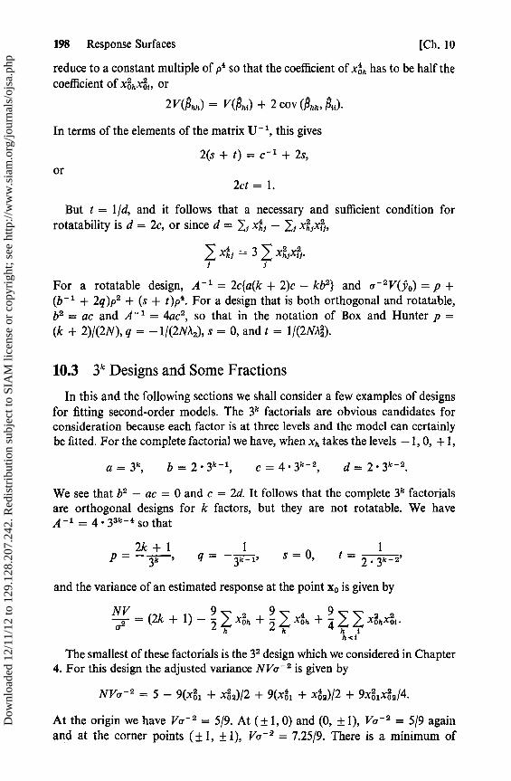
198 Response Surfaces [Ch. 10
reduce to a constant multiple of p4 so that the coefficient of xóh has to be half thecoefficient of xáhxo i, or
2 V(, hh) = V(h) + 2 COV (, hh, nu).
In terms of the elements of the matrix U 1 , this gives
2(s+t)=c - '+ 2s,or
2ct = 1.
But t = 1/d, and it follows that a necessary and sufficient condition forrotatability is d = 2c, or since d = JJ xh4 — ^J xhJx,1,
xh1 = 3 1 xhj j.J i
For a rotatable design, A -1 = 2c{a(k + 2)c — kb 2} and a -2 V(j 0) = p +(b - ' + 2q)p2 + (s + t)p4 . For a design that is both orthogonal and rotatable,b2 = ac and A -1 = 4ac 2, so that in the notation of Box and Hunter p =(k + 2)/(2N), q = —1/(2NA2), s = 0, and t = 1/(2N\).
10.3 31c Designs and Some FractionsIn this and the following sections we shall consider a few examples of designs
for fitting second-order models. The 3k factorials are obvious candidates forconsideration because each factor is at three levels and the model can certainlybe fitted. For the complete factorial we have, when x h takes the levels —1, 0, + 1,
a=3k , b = 2.3k -1 , c= 4.3k-2, d = 2.3k -2 .
We see that b 2 — ac = 0 and c = 2d. It follows that the complete 3k factorialsare orthogonal designs for k factors, but they are not rotatable. We haveA - ' = 4.33k -4 so that
p- 2k3 1 ^ q= —3k1 1, s=0,t=2.3k-a'
and the variance of an estimated response at the point x o is given by
áá = (2k + 1) — 2 xóh -I- xóh + 4 xónxóih<f
The smallest of these factorials is the 3 2 design which we considered in Chapter4. For this design the adjusted variance NVa -2 is given by
NVa - 2 = 5 — 9(x041 + xóa)/2 + 9(4 i + x042)/2 + 9xó1xóz/4 .
At the origin we have Vo -2 = 5/9. At (± 1, 0) and (0, ± 1), Vo -2 = 5/9 againand at the corner points (± 1, ± 1), Va -2 = 7.25/9. There is a minimum of
Dow
nloa
ded
12/1
1/12
to 1
29.1
28.2
07.2
42. R
edis
trib
utio
n su
bjec
t to
SIA
M li
cens
e or
cop
yrig
ht; s
ee h
ttp://
ww
w.s
iam
.org
/jour
nals
/ojs
a.ph
p

Sec. 10.3] 3k Designs and Some Fractions 199
3.2/9 at (± 0.4, ± 0.4). Box and Hunter (1957) give diagrams for the variancecontours for three designs for k = 2. The first of these is the 3 2 design, in whichthey have scaled the factors so that x1 = 4 = 9, i.e., the levels of Xh are— \/(3/2), 0, +-,/(3/2). The third design is the 3 2 factorial rotated through 45 0
,
and the second is one of the polygonal designs that will be considered in the nextsection.
For the 3 3 design we shall write v = NVa -2 . At the origin we have v = 7;at the center points of the faces of the cube, v = 7; at the midpoints of theedges, v = 9.25; and at the corners, v = 13.75. The minimum value of v occurswhen 1 = 4 = 4 = 1/3 and is 4.75. For any radius p the minimum varianceoccurs on the main diagonals of the cube.
We are again faced with the fact that there are twenty-seven points in the 3 3
design and only ten coefficients in the second-order equation. Debaun (1959)presents lome fractions of the 3 3 design. These are quite different from thefractions based upon hyperplanes that we considered in the previous chapter;those fractions are of little help to us in the present situation. Other designsbased on fractions of 3'1 factorials are given by Box and Behnken (1960).
Debaun considers five subsets of the complete factorial, each of which issymmetrical about the origin. They are
(i) The complete factorial;(ii) The cube with points (± 1, ± 1, ± 1);
(iii) The center point (0, 0, 0);(iv) The octahedron with points (± 1, 0, 0), (0, ± 1, 0), and (0, 0, ± 1) at the
centers of the faces of the cube;(v) The cuboctahedron, whose twelve points are the midpoints of the edges
of the cube given by (± 1, ±1,0),(±1,0, ± 1), and (0, ±1, ±1).
He goes on to consider and compare designs made by combining these fractions.The designs that he considers are
(i) The complete factorial;(ii) Cube plus octahedron plus n center points;
(iii) Cube plus 2 octahedra plus n center points;(iv) Cuboctahedron plus n center points;(v) Cube plus cuboctahedron plus n center points;
(vi) Cuboctahedron plus octahedron plus n center points.
In comparing the designs he uses as his criterion the information per point,which is v -1 . He shows that the complete factorial is a relatively inefficient designby this criterion and recommends designs (iii) and (iv). We shall now considerdesign (iv) and give an example.
The CuboctahedronFor the cuboctahedron with n center points we have N = a + 12 + n,
b=8,c=4,d= 4,andA-'=64n.
Dow
nloa
ded
12/1
1/12
to 1
29.1
28.2
07.2
42. R
edis
trib
utio
n su
bjec
t to
SIA
M li
cens
e or
cop
yrig
ht; s
ee h
ttp://
ww
w.s
iam
.org
/jour
nals
/ojs
a.ph
p

200 Response Surfaces [Ch. 10
If there are no center points the design is singular. If, however, n > 0, wehave
1 1 _ 4 —n _1p n' q __ 2n' S= 16n ' t 4'
and the design is orthogonal if, and only if, n = 4.In that case we have
v=4— 27xh +4 >xh +4(xlx2 +4 3+44).
Schneider and Stockett (1963) give an example of a cuboctahedron with threecenter points. The experiment was designed to determine the effects of columntemperature (z 1), gas/liquid ratio (z2), and packing height (z3) in reducing theunpleasant odor of a chemical product that was being sold for household use.The coded factors are
z 1 -80 z2 -0.5 z3 -4=xl40 ' x2 _ 0.2 ' x3 = 2
The second-order model
y = NO + N1x1 + N2x2 + P3x3 + Nll4 + P224 + jS33x32
+ P12x1x2 + P13x1x3 + P23x2x3
was fitted to the data. Afterwards the authors replaced x2 by x4 , which is theratio of liquid rate to packing height, and obtained a somewhat better fit(although it was still far from ideal). The three center points provide an unbiasedestimate of error with two degrees of freedom. The data and the analysis ofvariance table follow.
y x1 X2 X3 X4
66 —1 —1 0 11.7539 +1 —1 0 11.7543 —1 +1 0 3.7549 +1 +1 0 3.7558 —1 0 —1 11.0017 +1 0 —1 11.00
—5 —1 0 +1 3.67—40 +1 0 +1 3.67
65 0 —1 —1 23.507 0 +1 —1 7.50
43 0 —1 +1 7.80—22 0 +1 +1 2.50—31 0 0 0 5.50—35 0 0 0 5.50—26 0 0 0 5.50
Dow
nloa
ded
12/1
1/12
to 1
29.1
28.2
07.2
42. R
edis
trib
utio
n su
bjec
t to
SIA
M li
cens
e or
cop
yrig
ht; s
ee h
ttp://
ww
w.s
iam
.org
/jour
nals
/ojs
a.ph
p

Sec. 10.4] Polygonal Designs for k = 2 201
TABLE 10.1ANALYSIS OF VARIANCE
Source SS d.f. MS F
Raw Total 24,874.0 15Mean 129.1 1Corrected total 24,744.9 14First-order terms 17,940.2 3 5,980 295Second-order terms 5,253.3 6 876 44Lack of fit 1,510.7 3 504 25Error 40.7 2 20
10.4 Polygonal Designs for k = 2
A useful first-order design for two factors consists of the vertices of a regularpolygon with n sides inscribed in the unit circle. Each point in the design may beexpressed by x l = cos 6, x2 = sin 0, where 0 is the angle between the radiusvector and the x l axis. Taking the first point to be x l = 1, x2 = 0, the otherpoints correspond to 0 = 2jir/n, j = 1, 2, ... , n — 1;x 1 + ix2 = cos 6 + i sin 0are the roots of the equation xn — 1 = 0 with (1, 0) corresponding to j = n.
The sum of the roots of x' — 1 = 0 is zero. Hence, 1?n 1 cos 0 + i sin 0 = 0so that 1 cos 0 = 1 sin 6 = 0 and xfl = 1 xj2 = 0. Furthermore, the sum ofthe squares of the roots is also zero. Hence,
(cos 0 + i sin 9) 2 = cos2 8 — sine 0 + 2i 1 sin 0 cos 0 = 0.
Also, 7, cos2 0 + 1 sine 0 = n. We thus have
xil = 4 = cos 2 0 = 1 sine 6 = n/2;
1 xjlxf2 = 1 sin 0 cos 6 = 0.
The first-order design is orthogonal and satisfies the conditions that we imposedon first-order designs in the previous sections. It is easily shown that the designretains these properties if it is rotated through any angle a, i.e., if xfl = cos(a + 2jwln) and x52 = sin (a + 2jrr/n). A larger design may be made up by usingseveral polygons and letting the hth polygon have nh vertices and radius Ph; inparticular, we may add no center points at the origin.
When we turn to second-order designs we note that for the single polygon4 + xiz - 1 at each point, and the design is singular. Suppose that we add no
center points and let N = n + no . It is necessary that n > 5.
Dow
nloa
ded
12/1
1/12
to 1
29.1
28.2
07.2
42. R
edis
trib
utio
n su
bjec
t to
SIA
M li
cens
e or
cop
yrig
ht; s
ee h
ttp://
ww
w.s
iam
.org
/jour
nals
/ojs
a.ph
p

202 Response Surfaces [Ch. 10
The sum of the cubes of the roots of xn = 1 is zero. Hence,
1 (cos3 0 — 3 sin' 0 cos 6) + i 1. (3 sin 0 cos2 0 — cos3 0) = 0.
But (cos3 0 — 3 sine 0 cos B) = 4 cos3 0 — 3 cos 0, and we have
1 cos3 6 = 1 sin3 6 = cos2 6 sin 0 = 1 cos 0 sine 0 = 0.
The sum of the fourth powers also vanishes, giving cos 3 0 sin 0 = cos 0sin3 0 = 0, and also 1(cos 4 6 + sin4 6 — 6 cos 2 6 sine 6) = 0. But
(cos2 6 + sin2 6)2 = (cos4 6 + sin4 6 + 2 cos2 6 sine 6) = n;
hence,
1 sine 6 cos2 6 = n/8.
Furthermore,
cos4 0 = cos2 6(1 — sine 6) = n/2 — n/8 = 3n/8 = sin4 6.
In the notation of the previous section, we now have
a = N = n + n o , b = n/2, c = n/8, d = n/4.
It is not surprising that the rotatability condition d = 2c is satisfied. Theorthogonality condition b2 = ac leads to
n2/4 = (n + no)n/8, or n = no ,
which calls for more center points than many experimenters might regard aspracticable. The elements of the covariance matrix are
p=n5 1 , q=—no 1 , s= nol—n -1 , t =4n -1 .
The variance of the estimate of the response at a point a distance p from theorigin is given by
o_2 V(9) = n' + (2n -1 — 2n0')p2 + (nó 1 + 3n 1)p4 .
If the design is orthogonal, this becomes
a -2 V(ƒ) = n -1(1 + 4p4),
and the minimum variance occurs at the origin.
Dow
nloa
ded
12/1
1/12
to 1
29.1
28.2
07.2
42. R
edis
trib
utio
n su
bjec
t to
SIA
M li
cens
e or
cop
yrig
ht; s
ee h
ttp://
ww
w.s
iam
.org
/jour
nals
/ojs
a.ph
p
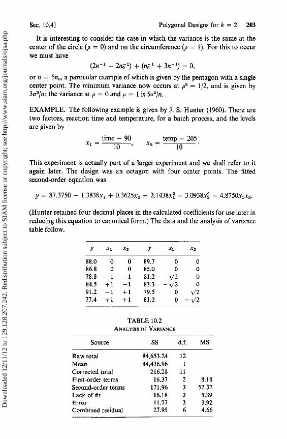
Sec. 10.4] Polygonal Designs for k = 2 203
It is interesting to consider the case in which the variance is the same at thecenter of the circle (p = 0) and on the circumference (p = 1). For this to occurwe must have
(2n -1 - 2no') + (no' + 3n -1) = 0,
or n = 5n 0 , a particular example of which is given by the pentagon with a singlecenter point. The minimum variance now occurs at p2 = 1/2, and is given by3a2/n; the variance at p = 0 and p = 1 is 5o2/n.
EXAMPLE. The following example is given by J. S. Hunter (1960). There aretwo factors, reaction time and temperature, for a batch process, and the levelsare given by
time -90 temp - 205xl = 10 , x2 = 10
This experiment is actually part of a larger experiment and we shall refer to itagain later. The design was an octagon with four center points. The fittedsecond-order equation was
y = 87.3750 - 1.3838x1 + 0.3625x 2 - 2.14384 - 3.09384 - 4.8750x 1x2 .
(Hunter retained four decimal places in the calculated coefficients for use later inreducing this equation to canonical form.) The data and the analysis of variancetable follow.
Y Xl X2 Y xi X2
88.0 0 0 89.7 0 086.8 0 0 85.0 0 078.8 -1 -1 81.2 /2 084.5 +1 -1 83.3 -\/2 091.2 -1 +1 79.5 0 /277.4 +1 +1 81.2 0 -\/2
TABLE 10.2ANALYSIS OF VARIANCE
Source SS d.f. MS
Raw total 84,653.24 12Mean 84,436.96 1Corrected total 216.28 11First-order terms 16.37 2 8.18Second-order terras 171.96 3 57.32Lack of fit 16.18 3 5.39Error 11.77 3 3.92Combined residual 27.95 6 4.66
Dow
nloa
ded
12/1
1/12
to 1
29.1
28.2
07.2
42. R
edis
trib
utio
n su
bjec
t to
SIA
M li
cens
e or
cop
yrig
ht; s
ee h
ttp://
ww
w.s
iam
.org
/jour
nals
/ojs
a.ph
p
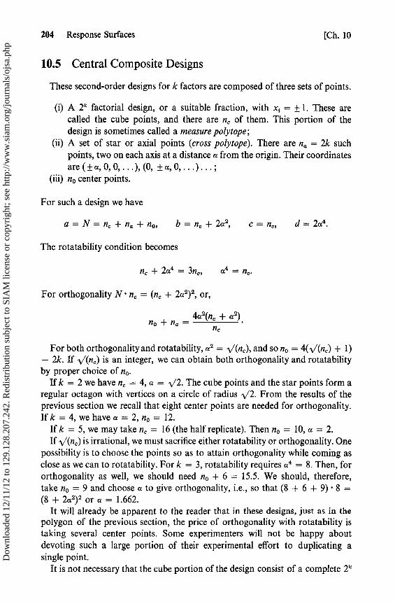
204 Response Surfaces [Ch. 10
10.5 Centra! Composite Designs
These second-order designs for k factors are composed of three sets of points.
(i) A 2' factorial design, or a suitable fraction, with x { = ± 1. These arecalled the cube points, and there are n, of them. This portion of thedesign is sometimes called a measure polytope;
(ii) A set of star or axial points (cross polytope). There are na = 2k suchpoints, two on each axis at a distance a from the origin. Their coordinatesare (± a, 0, 0, ... ), (0, ± a,
(iii) no center points.
For such a design we have
a=N=nc +na +no , b=n,+2a2, c=nc , d=2a4 .
The rotatability condition becomes
n, + 2a4 = 3n^, a4 = n,.
For orthogonality N • n, = (n, + 2a 2)2, or,
4a2(n + a2)no +na =nc
For both orthogonality and rotatability, a 2 = -s/(n), and so no = 4('./(n,) + 1)— 2k. If -,/(n,) is an integer, we can obtain both orthogonality and rotatabilityby proper choice of n o .
If k = 2 we have nc = 4, a = -,/2. The cube points and the star points form aregular octagon with vertices on a circle of radius -,/2. From the results of theprevious section we recall that eight center points are needed for orthogonality.If k = 4, we have a = 2, n o = 12.
If k = 5, we may take nc = 16 (the half replicate). Then n o = 10, a = 2.If -,/(n c) is irrational, we must sacrifice either rotatability or orthogonality. One
possibility is to choose the points so as to attain orthogonality while coming asclose as we can to rotatability. For k = 3, rotatability requires a 4 = 8. Then, fororthogonality as well, we should need n o + 6 = 15.5. We should, therefore,take no = 9 and choose a to give orthogonality, i.e., so that (8 + 6 + 9) • 8 =(8 + 2a2)2 or a = 1.662.
It will already be apparent to the reader that in these designs, just as in thepolygon of the previous section, the price of orthogonality with rotatability istaking several center points. Some experimenters will not be happy aboutdevoting such a large portion of their experimental effort to duplicating asingle point.
It is not necessary that the cube portion of the design consist of a complete 2'
Dow
nloa
ded
12/1
1/12
to 1
29.1
28.2
07.2
42. R
edis
trib
utio
n su
bjec
t to
SIA
M li
cens
e or
cop
yrig
ht; s
ee h
ttp://
ww
w.s
iam
.org
/jour
nals
/ojs
a.ph
p

Sec. 10.5] Central Composite Designs 205
design; the use of the half replicate has already been mentioned. In seeking toreduce the number of points in a composite design, we may note that theresponse at a center point estimates Po ; the difference between the average of theresponses at the two star points on the ith axis and the average at the centerpoints gives an estimate of fl, and the difference between the responses at thetwo axial points gives an estimate of 2afl,. Thus the center points and the starpoints give estimates of all but the interaction terms fl,, and the Jatter have to beestimated from the cube points. We may therefore use a fraction, if there is onethat will allow all two-factor interactions to be estimated, assuming the maineffects to be known. If we are prepared to suppress all interactions with three ormore factors, we may thus use any 2k - ' fraction that contains no more than one2 f.i. in any alias set. (If there is a single 2 f.i. among the defining contrasts, thatwill contradict our simplifying assumption that 1 XjhXji = 0 for all pairs andcomplicate the calculations, but the parameters will still be estimable.) Hartley(1959) suggests using, when k = 6, the quarter replicate defined by I = ABC =DEF = ABCDEF. Consider, for example, the AB contrast. If we suppresshigher order interactions, its expectation is 16(fl 12 + fl), and we already have anestimate of f3 from the star points.
Aia, et al. (1961) used a central composite design with k = 3, a = 1.6818, andsix center points in an experiment on the precipitation of stoichiometric di-hydrate of calcium hydrogen orthophosphate (CaHPO 4 .2H2O). Among theresponses that they considered was the percentage yield. The three factors usedwere the mole ratio of NH 3 to CaC12 in the calcium chloride solution, theaddition time in minutes of the NH 3-CaCl 2 mix, and the starting pH of theNH4H2PO4 solution used.
The scaled factors were
xl = [(NH3) /(CaC12) — 0.85]/0.09, x2 = (t — 50)/24,
x3 = (pH — 3.5)/0.9.
The fitted second-order equation was
y = 76.03 + 5.49x 1 — 0.71x2 + 10.18x3 — 0.88x 1 x2 — 1.46x1x3 — 0.29x2x3
+0.694 + 0.432 — 7.18x3.
They later decided to drop the x 2 terms from the model. The new fitted equationwas then
= 76.39 + 5.49x 1 + 10.18x3 — 1.46x 1x3 + 0.644 — 7.22x3.
The changes in the quadratic coefficients and the constant term when x 2 isomitted are small. There is no change in the coefficients of x l and x3 becausethese terms are orthogonal to the x 2 term and the other terms.
Dow
nloa
ded
12/1
1/12
to 1
29.1
28.2
07.2
42. R
edis
trib
utio
n su
bjec
t to
SIA
M li
cens
e or
cop
yrig
ht; s
ee h
ttp://
ww
w.s
iam
.org
/jour
nals
/ojs
a.ph
p

206 Response Surfaces [Ch. 10
The data and the analysis of variance table follow.
X1 X2 X3 Y X1 X2 X3 Y
-1 -1 -1 52.8 0 -1.6818 0 80.61 -1 -1 67.9 0 +1.6818 0 77.5
-1 1 -1 55.4 0 0 -1.6818 36.81 1 -1 64.2 0 0 + 1.6818 78.0
-1 -1 1 75.1 0 0 0 74.61 -1 1 81.6 0 0 0 75.9
-1 1 1 73.8 0 0 0 76.91 1 1 79.5 0 0 0 72.3
-1.6818 0 0 68.1 0 0 0 75.9+1.6818 0 0 91.2 0 0 0 79.8
TABLE 10.3ANALYSIS OF VARIANCE
Source SS d.f.
Total 770.96 19First-order terms 610.93 3Second-order terms 135.15 6Lack of fit 18.71 5Error 6.17 5
10.6 Orthogonal Blocking
We now discuss breaking up the response surface design into m blocks;the wth block contains nw points. The block effects are additive constants, andthere is no interaction between blocks and factors. We may modify our modelaccordingly and write
E(Y5) = PO + Po.(ziw - Zw) + 1 Nhxih + PhiXn XJI + 1 Nhhxjh,w=1 h h t h
h«
where Po + PO is the expected response at the origin in the wth block; Sow is thewth block effect, and we impose the side condition Lw flownw = 0; zfw is a dummyvariable which takes the value + 1 if the jth point is in the wth block, and iszero otherwise. We denote by zw the average n,,/N.
It is desirable that the block effects be orthogonal to the parameters of theresponse surface. This is achieved if, and only if, the corresponding designvectors are perpendicular, i.e., if for each w
(Zlw - zW)xlh = 0 (10.6)Dow
nloa
ded
12/1
1/12
to 1
29.1
28.2
07.2
42. R
edis
trib
utio
n su
bjec
t to
SIA
M li
cens
e or
cop
yrig
ht; s
ee h
ttp://
ww
w.s
iam
.org
/jour
nals
/ojs
a.ph
p
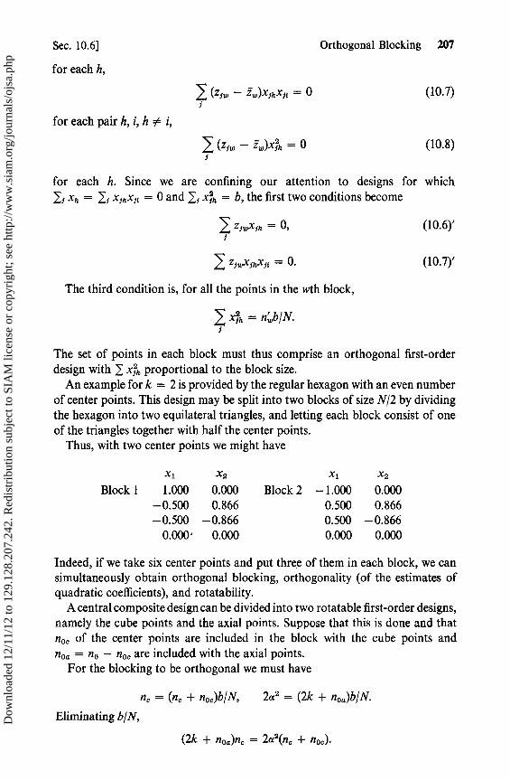
Sec. 10.6] Orthogonal Blocking 207
for each h,
(z5, — ZW)xlhxfi = 0 (10.7)
for each pair h, i, h i,
(Z!w - i.)XJh = 0 (10.8)
for each h. Since we are confining our attention to designs for which
! xh = I! xlhxlt = 0 and I! 4,, = b, the first two conditions become
Zlwxlh = 0, (10.6)'!
1 Zlwxlhxlt = 0. (10.7)'
The third condition is, for all the points in the wth block,
xƒh = n,,b/N.
The set of points in each block must thus comprise an orthogonal first-orderdesign with 1 xih proportional to the block size.
An example for k = 2 is provided by the regular hexagon with an even numberof center points. This design may be split into two blocks of size N/2 by dividingthe hexagon into two equilateral triangles, and letting each block consist of oneof the triangles together with half the center points.
Thus, with two center points we might have
xl x2 xl x2
Block 1 1.000 0.000 Block 2 —1.000 0.000—0.500 0.866 0.500 0.866—0.500 —0.866 0.500 —0.866
0.0001 0.000 0.000 0.000
Indeed, if we take six center points and put three of them in each block, we cansimultaneously obtain orthogonal blocking, orthogonality (of the estimates ofquadratic coefficients), and rotatability.
A central composite design can be divided into two rotatable first-order designs,namely the cube points and the axial points. Suppose that this is done and thatnoc of the center points are included in the block with the cube points andnoa = n o — noc are included with the axial points.
For the blocking to be orthogonal we must have
nc = (nc + noc)b/N, 2a2 = (2k + noa)b/N.
Eliminating b/N,
(2k + noa)nc = 2_2(n0 + noc)•
Dow
nloa
ded
12/1
1/12
to 1
29.1
28.2
07.2
42. R
edis
trib
utio
n su
bjec
t to
SIA
M li
cens
e or
cop
yrig
ht; s
ee h
ttp://
ww
w.s
iam
.org
/jour
nals
/ojs
a.ph
p

208 Response Surfaces [Ch. 10
A convenient example is the case k = 4 and n, = 16. We have already seen thatfor orthogonality and rotatability no = 12 and a2 = 4. Orthogonal blocking isthen obtained by putting no, = 8 and noa = 4.
The cube points may be divided into two half replicates confounding the four-factor interaction. Each half replicate is an orthogonal first-order design, and sowe can add four center points to each 2 -1 and thereby have a design for n =16 + 8 + 12 = 36 divided into three orthogonal blocks of twelve points each.
The octagonal design with four center points given as an example in thesection on polygonal designs can be run in two orthogonal blocks. The blockscorrespond to the columns in the listing of the data. If we consider the octagonaldesign as a central composite design for k = 2 with a = 4 and n, = 4, the firstblock consists of the "cube" points together with two center points. The secondblock contains the star points plus the two remaining center points.
10.7 Steepest Ascent and Canonical Equations
So far we have talked about designs for fitting first- and second-order modelswithout concerning ourselves about the problem of where or when to fit them.It will be convenient for us to confine ourselves for the moment to two factors,xl and x2 i the generalization to k factors will be clear. How do we decide aboutthe levels of the factors? There are two points to be remembered.
1. We are not really concerned about investigating the response over theentire sample spare of points (x1 , x2) at which the plant will operate. We areinterested only in operating in the subset of the sample space in which theresponse is optimized. The term optimizing the response is not as simple as itsounds. In a practical situation there may be confusion over what response is tobe optimized. The engineer wishes to optimize the yield of some product. Thecomptroller's department employees in the head office have in mind optimizingprofit, and they may calculate it by a formula unknown to the researchera.There are, for example, some situations in which it is better to maximizethe total yield than the percentage yield. It might, perhaps, be more desir-able to pass 200 gallons of feed stock per hour through a plant converting only60 per cent, than to pass 100 gallons per hour with 80 per cent conversion. Forconvenience we shall think in terms of maximizing conversion or yield, recogniz-ing, however, that in some cases other responses may be of greater interest.
If we are interested in running the plant in the area of maximum yield, thenwe are interested only in investigating closely the area of the sample space inwhich the yields are high. We do not care to devote any more time than isnecessary to exploring regions of no economic interest. We envision a two-dimensional factor space, with the yield as the third dimension rising out of thex1 , x2 plane. Hopefully, this three-dimensional figure y = f(x l , x2) has a singlepeak, and we would like to find it. Having found it we shall operate the plant atthose conditions, and the stockholders will be content. Perhaps the peak isunattainable—it might require so high a temperature that we should burst aboiler—but we shall do the best we can.
Dow
nloa
ded
12/1
1/12
to 1
29.1
28.2
07.2
42. R
edis
trib
utio
n su
bjec
t to
SIA
M li
cens
e or
cop
yrig
ht; s
ee h
ttp://
ww
w.s
iam
.org
/jour
nals
/ojs
a.ph
p
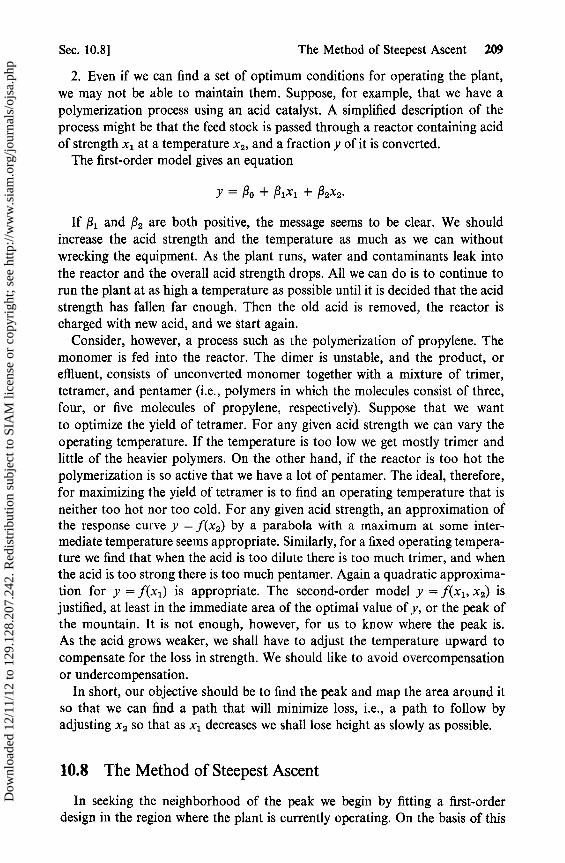
Sec. 10.8] The Method of Steepest Ascent 209
2. Even if we can find a set of optimum conditions for operating the plant,we may not be able to maintain them. Suppose, for example, that we have apolymerization process using an acid catalyst. A simplified description of theprocess might be that the feed stock is passed through a reactor containing acidof strength xl at a temperature x 2 , and a fraction y of it is converted.
The first-order model gives an equation
Y = No + Nlxl + N2x2.
If /3 and P2 are both positive, the message seems to be clear. We shouldincrease the acid strength and the temperature as much as we can withoutwrecking the equipment. As the plant runs, water and contaminants leak intothe reactor and the overall acid strength drops. All we can do is to continue torun the plant at as high a temperature as possible until it is decided that the acidstrength has fallen far enough. Then the old acid is removed, the reactor ischarged with new acid, and we start again.
Consider, however, a process such as the polymerization of propylene. Themonomer is fed into the reactor. The dimer is unstable, and the product, oreffluent, consists of unconverted monomer together with a mixture of trimer,tetramer, and pentamer (i.e., polymers in which the molecules consist of three,four, or five molecules of propylene, respectively). Suppose that we wantto optimize the yield of tetramer. For any given acid strength we can vary theoperating temperature. If the temperature is too low we get mostly trimer andlittle of the heavier polymers. On the other hand, if the reactor is too hot thepolymerization is so active that we have a lot of pentamer. The ideal, therefore,for maximizing the yield of tetramer is to find an operating temperature that isneither too hot nor too cold. For any given acid strength, an approximation ofthe response curve y = f(x2) by a parabola with a maximum at some inter-mediate temperature seems appropriate. Similarly, for a fixed operating tempera-ture we find that when the acid is too dilute there is too much trimer, and whenthe acid is too strong there is too much pentamer. Again a quadratic approxima-tion for y = f(x 1) is appropriate. The second-order model y = f(x1 , x2) isjustified, at least in the immediate area of the optimal value of y, or the peak ofthe mountain. It is not enough, however, for us to know where the peak is.As the acid grows weaker, we shall have to adjust the temperature upward tocompensate for the loss in strength. We should like to avoid overcompensationor undercompensation.
In short, our objective should be to find the peak and map the area around itso that we can find a path that will minimize loss, i.e., a path to follow byadjusting x2 so that as x l decreases we shall lose height as slowly as possible.
10.8 The Method of Steepest Ascent
In seeking the neighborhood of the peak we begin by fitting a first-orderdesign in the region where the plant is currently operating. On the basis of this
Dow
nloa
ded
12/1
1/12
to 1
29.1
28.2
07.2
42. R
edis
trib
utio
n su
bjec
t to
SIA
M li
cens
e or
cop
yrig
ht; s
ee h
ttp://
ww
w.s
iam
.org
/jour
nals
/ojs
a.ph
p
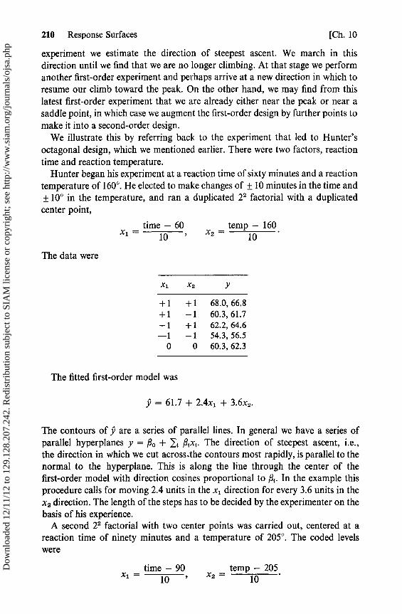
210 Response Surfaces [Ch. 10
experiment we estimate the direction of steepest ascent. We march in thisdirection until we find that we are no longer climbing. At that stage we performanother first-order experiment and perhaps arrive at a new direction in which toresume our climb toward the peak. On the other hand, we may find from thislatest first-order experiment that we are already either near the peak or near asaddle point, in which case we augment the first-order design by further points tomake it into a second-order design.
We illustrate this by referring back to the experiment that led to Hunter'soctagonal design, which we mentioned earlier. There were two factors, reactiontime and reaction temperature.
Hunter began his experiment at a reaction time of sixty minutes and a reactiontemperature of 160°. He elected to make changes of ± 10 minutes in the time and± 10 ° in the temperature, and ran a duplicated 2 2 factorial with a duplicatedcenter point,
_ time — 60 temp — 160xl 10 x2
_ 10
The data were
xi x2 Y
+1 +1 68.0, 66.8
+1 —1 60.3,61.7
—1 +1 62.2, 64.6
—1 —1 54.3, 56.5
0 0 60.3, 62.3
The fitted first-order model was
5' =61.7 +2.4x1 +3.6x2 .
The contours of y are a series of parallel lines. In general we have a series ofparallel hyperplanes y = /3 + 1, Pix; . The direction of steepest ascent, i.e.,the direction in which we cut across.the contours most rapidly, is parallel to thenormal to the hyperplane. This is along the live through the center of thefirst-order model with direction cosines proportional to Pt . In the example thisprocedure calls for moving 2.4 units in the x l direction for every 3.6 units in thex2 direction. The length of the steps has to be decided by the experimenter on thebasis of his experience.
A second 22 factorial with two center points was carried out, centered at areaction time of ninety minutes and a temperature of 205 °. The coded levelswere
time —90 temp — 205x1 = 10 , x2 = 10
Dow
nloa
ded
12/1
1/12
to 1
29.1
28.2
07.2
42. R
edis
trib
utio
n su
bjec
t to
SIA
M li
cens
e or
cop
yrig
ht; s
ee h
ttp://
ww
w.s
iam
.org
/jour
nals
/ojs
a.ph
p
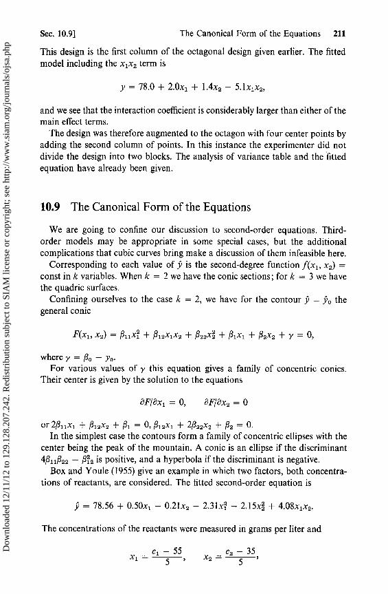
Sec. 10.9] The Canonical Form of the Equations 211
This design is the first column of the octagonal design given earlier. The fittedmodel including the x1x2 term is
y = 78.0 + 2.0x 1 + 1.4x2 — 5.1x 1x2 ,
and we see that the interaction coefficient is considerably larger than either of themain effect terms.
The design was therefore augmented to the octagon with four center points byadding the second column of points. In this instance the experimenter did notdivide the design into two blocks. The analysis of variance table and the fittedequation have already been given.
10.9 The Canonical Form of the Equations
We are going to confine our discussion to second-order equations. Third-order models may be appropriate in lome special cases, but the additionalcomplications that cubic curves bring make a discussion of them infeasible here.
Corresponding to each value of y is the second-degree function f(x l , x2) =const in k variables. When k = 2 we have the conic sections; for k = 3 we havethe quadric surfaces.
Confining ourselves to the case k = 2, we have for the contour y = yo thegeneral conic
F(x1, x2) = N11x1 + ,812x1x2 + 822x2 + fl 1x1 + P2x2 + y = 0,
where y = Po — Yo•For various values of y this equation gives a family of concentric conics.
Their center is given by the solution to the equations
aF/8x 1 = 0, aF/8x2 = 0
or 211x1 + P12x2 + Nl = 0,12x1 + 2P22x2 + N2 = 0 •In the simplest case the contours form a family of concentric ellipses with the
center being the peak of the mountain. A conic is an ellipse if the discriminant4 11f22 — P2 is positive, and a hyperbola if the discriminant is negative.
Box and Youle (1955) give an example in which two factors, both concentra-tions of reactants, are considered. The fitted second-order equation is
= 78.56 + 0.50x1 — 0.21x2 — 2.312 — 2.15x2 + 4.08x1x2 .
The concentrations of the reactants were measured in grams per liter and
c1 -55 c2-35xl =5 , x2 = 5
Dow
nloa
ded
12/1
1/12
to 1
29.1
28.2
07.2
42. R
edis
trib
utio
n su
bjec
t to
SIA
M li
cens
e or
cop
yrig
ht; s
ee h
ttp://
ww
w.s
iam
.org
/jour
nals
/ojs
a.ph
p
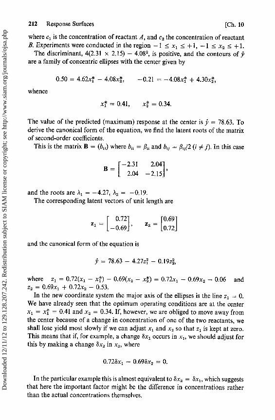
212 Response Surfaces [Ch. 10
where cl is the concentration of reactant A, and c2 the concentration of reactantB. Experiments were conducted in the region —1 < x l < +1, —1 < x2 < + 1.
The discriminant, 4(2.31 x 2.15) — 4.08 2, is positive, and the contours of 9are a family of concentric ellipses with the center given by
0.50 = 4.624' — 4.084, —0.21 = —4.084' + 4.304,
whence
xi = 0.41, 4 = 0.34.
The value of the predicted (maximum) response at the center is 9 = 78.63. Toderive the canonical form of the equation, we find the latent roots of the matrixof second-order coefficients.
This is the matrix B = (b;j) where bi; = fl and bi; = fl/2 (i j). In this case
[-2.31 2.04B—
2.04 —2.15]'
and the roots are A l = —4.27, ,12 = — 0.19.The corresponding latent vectors of unit length are
Zl = 1-0.69, 'Z Z = [0.
and the canonical form of the equation is
y = 78.63 — 4.27zi — 0.194
where zl = 0.72(x 1 — xi) — 0.69(x2 — 4') = 0.72x1 — 0.69x2 — 0.06 andz2 = 0.69x1 + 0.72x2 — 0.53.
In the new coordinate system the major axis of the ellipses is the live zl = 0.We have already seen that the optimum operating conditions are at the centerxl = x = 0.41 and x2 = 0.34. If, however, we are obliged to move away fromthe center because of a change in concentration of one of the two reactants, weshall lose yield most slowly if we can adjust x l and x2 so that zl is kept at zero.This means that if, for example, a change 8x 1 occurs in x 1 , we should adjust forthis by making a change Sx 2 in x2 , where
0.728x1 — 0.698x2 = 0.
In the particular example this is almost equivalent to 8x 2 = 8x1 , which suggeststhat here the important factor might be the difference in concentrations ratherthan the actual concentrations themselves.
Dow
nloa
ded
12/1
1/12
to 1
29.1
28.2
07.2
42. R
edis
trib
utio
n su
bjec
t to
SIA
M li
cens
e or
cop
yrig
ht; s
ee h
ttp://
ww
w.s
iam
.org
/jour
nals
/ojs
a.ph
p

Sec. 10.11]
Evolutionary Operation 213
10.10 Other Surfaces
In the example given by Hunter the second-order equation was
9 = 87.3750 — 1.3838x 1 + 0.3625x2 — 2.1438x1 — 3.0938x2 — 4.8750x 1x2 .
This is allo a family of ellipses, but in this case the center is at x l = — 3.7369,x2 = + 3.0028, which is well outside the area of experimentation. It may evenbe outside the range in which the plant can be operated. In the area where theexperiments took place the response surface is a rising ridge, and further experi-mentation might take place in the direction of a line toward the center.
The canonical form is
y = 90.50 — 5.10z1 — 0.14zá,
where zl = 0.64x 1 + 0.77x2 + 0.06 and z2 = — 0.77x 1 + 0.64x2 — 4.79. In-creases in the value of zi bring about sharp decreases in the yield.
When the contours are hyperbolas, the response surface is a saddle surfacewith the center of the family at the center of the saddle. Moving away from thecenter along one of the axes will produce an increase in the yield. Moving awayalong the other axis will result in a drop in the yield. The experiment by Aia et al.(1961) gave a saddle surface.
As the discriminant approaches zero, the family of curven approaches afamily of degenerate parabolas, and the contours become a series of pairs ofparallel lines. This is a ridge surface, and the optimum procedure would be tofind the highest of the parallel ridges and to remain on it.
With three factors the geometrical representation becomes more difficult.There are several worked examples in the literature, particularly in the paperby Box and Youle (1955) and the book by Davies (1956). Further examplesappear from time to time in chemical and agronomic journals. Examples ofthird- and fourth-order models are not found as often because the designs andthe interpretation of the results are, on the whole, too complicated for generaluse by engineers. Third- and fourth-order rotatable designs are discuseed byGardner, et al. (1959), and in a series of papers by Draper (1960a, b; 1961;1962).
10.11 Evolutionary Operation
The discussion so far has been concerned with the design of specific experi-ments, particularly with experiments that might be carried out in a pilot plant bya research and development group. Once an actual plant is in operation, littleexperimentation usually takes place. If the plant can be persuaded to operate
Dow
nloa
ded
12/1
1/12
to 1
29.1
28.2
07.2
42. R
edis
trib
utio
n su
bjec
t to
SIA
M li
cens
e or
cop
yrig
ht; s
ee h
ttp://
ww
w.s
iam
.org
/jour
nals
/ojs
a.ph
p

214 Response Surfaces [Ch. 10
under conditions that produce profitable yields, the attention of the operators isdirected toward keeping the plant working at those conditions and maintainingthe status quo. Perhaps it would be possible to improve the yield somewhat, but,on the other hand, tinkering around with the operating variables might cause adrop in production. This defensive approach is bolstered by the conviction thatthe research personnel will have to make large changes in the operating variablesin order to obtain meaningful results.
A new plant may produce at a lower yield than had been expected because ofproblems of scale up. If a plant to produce a thousand barrels a day is to bedesigned on the basis of a pilot plant that produces two barrels a day, somedimensions will have to be increased five hundred fold, some by \/5, and someby the cube root. When the actual plant is built, it may well happen that theactual optimum operating conditions are not those that were obtained on thepilot plant, and the yield will fall short of the projections. Little will be gained byasking the research staff to generate more data on the pilot plant. If they did areasonable job the first time, further data will only serve to confirm theirearlier results. What is needed at this stage is not more information about how torun the pilot plant but information about optimizing production on the full-sizeplant that has already been built.
Evolutionary operation was proposed by Box (1957) as an operating procedurefor nudging a plant toward optimum conditions without causing dramaticdisturbances and catastrophic cutbacks in production. It is designed as a methodof operation that can be carried out by the plant personnel themselves with aminimum of supervision, or interference, from the research people. Indeed, it isrecommended as a standard operating procedure, whether or not there is concernabout the performance of the plant.
An evolutionary operation program for a plant contains two basic steps:
(i) A routine of systematic small changes is introduced in the levels of theoperating variables being considered;
(ii) The information generated is fed back to the plant foreman or othersupervisor.
Box and Hunter (1959) show how the latter objective is facilitated by usingsimplified calculations and emphasizing graphical presentation. They give anexample of an application to a batch process in which the two operating variablesbeing monitored are temperature and reaction time. We shall use part of theirexample. There is nothing in the theory to prevent us from monitoring severalvariables but, for practical purposes, two or three variables are enough tohandle under normal circumstances. Box and Hunter also discuss the case inwhich three variables are monitored.
The operating cycle is a cycle of five points that form a 2 2 factorial with a centerpoint. If the plant is currently operating at a temperature of 120° with a reactiontime of sixty minutes, and if fluctuations of ± 10 ° in the temperature and ± 10
Dow
nloa
ded
12/1
1/12
to 1
29.1
28.2
07.2
42. R
edis
trib
utio
n su
bjec
t to
SIA
M li
cens
e or
cop
yrig
ht; s
ee h
ttp://
ww
w.s
iam
.org
/jour
nals
/ojs
a.ph
p

Sec. 10.11] Evolutionary Operation 215
minutes in the time are contemplated, the cycle would consist of the five points
120°, 60 min;110°, 50 min;130°, 70 min;110°, 70 min;1300, 50 min.
The cycle is repeated several times. Each time the responses Y1, Y2, Ys, Y4, Y5
are recorded and their averages are posted. The main effects and the interactionof the two factors are calculated, and when one or more of these three effectsbecomes significant, decisions about changes in operating conditions are madeby the plant foreman.
The most important feature in step (ii) is the information board. Table 10.4
TABLE 10.4YIELDS DURING THE FIRST FOUR CYCLES
Conditions
Cycle 1 2 3 4 5
1 63.7 62.8 63.2 67.2 60.52 62.1 65.8 65.5 67.6 61.33 59.6 62.1 62.0 65.3 64.14 63.5 62.8 67.9 62.6 61.7
TABLE 10.5INFORMATION BOARD-CYCLE 4
Per cent yield Other ResponsesRequirement Maximize
1 61.9 64.6T,
E62.2M
P63.4 65.71-TIME-
Error Limits for Averages ± 2.3
Effects with time +2.5 ± 2.395% error temperature -1.3 ± 2.3Limits t x T 0.2 ± 2.3
Change in mean 1.4 ± 2.0
Standard deviation 2.3Prior estimate of o 1.8
Dow
nloa
ded
12/1
1/12
to 1
29.1
28.2
07.2
42. R
edis
trib
utio
n su
bjec
t to
SIA
M li
cens
e or
cop
yrig
ht; s
ee h
ttp://
ww
w.s
iam
.org
/jour
nals
/ojs
a.ph
p
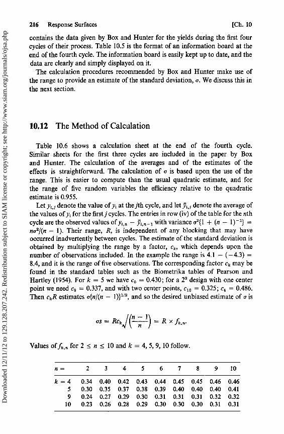
216 Response Surfaces [Ch. 10
contains the data given by Box and Hunter for the yields during the first fourcycles of their process. Table 10.5 is the format of an information board at theend of the fourth cycle. The information board is easily kept up to date, and thedata are clearly and simply displayed on it.
The calculation procedures recommended by Box and Hunter make use ofthe range to provide an estimate of the standard deviation, a. We discuss this inthe next section.
10.12 The Method of Calculation
Table 10.6 shows a calculation sheet at the end of the fourth cycle.Similar sheets for the first three cycles are included in the paper by Boxand Hunter. The calculation of the averages and of the estimates of theeffects is straightforward. The calculation of o is based upon the use of therange. This is easier to compute than the usual quadratic estimate, and forthe range of live random variables the efficiency relative to the quadraticestimate is 0.955.
Let yt , 1 denote the value of y i at thejth cycle, and let y,,, denote the average ofthe values of y i for the first ] cycles. The entries in row (iv) of the table for the nthcycle are the observed values of y j, - with variance a 2{1 + (n - 1) -1} =nat/(n - 1). Their range, R, is independent of any blocking that may haveoccurred inadvertently between cycles. The estimate of the standard deviation isobtained by multiplying the range by a factor, ck, which depends upon thenumber of observations included. In the example the range is 4.1 - (-4.3) =8.4, and it is the range of five observations. The corresponding factor c, may befound in the standard tables such as the Biometrika tables of Pearson andHartley (1954). For k = 5 we have c 5 = 0.430; for a 2 design with one centerpoint we need c 9 = 0.337, and with two center points, c lo = 0.325; c 4 = 0.486.Then ckR estimates a{n/(n - 1)} 112 , and so the desired unbiased estimate of a is
as = RCk, \n 1) = R x fk ,_.
Values of fk , fl for 2 < n < 10 and k = 4, 5, 9, 10 follow.
n= 2 3 4 5 6 7 8 9 10
k = 4 0.34 0.40 0.42 0.43 0.44 0.45 0.45 0.46 0.465 0.30 0.35 0.37 0.38 0.39 0.40 0.40 0.40 0.419 0.24 0.27 0.29 0.30 0.31 0.31 0.31 0.32 0.32
10 0.23 0.26 0.28 0.29 0.30 0.30 0.30 0.31 0.31
Dow
nloa
ded
12/1
1/12
to 1
29.1
28.2
07.2
42. R
edis
trib
utio
n su
bjec
t to
SIA
M li
cens
e or
cop
yrig
ht; s
ee h
ttp://
ww
w.s
iam
.org
/jour
nals
/ojs
a.ph
p

TA
BL
E10
.6C
AL
CU
LA
TIO
NS
HE
ET
-EN
DO
FF
OU
RC
YC
LE
S
Cal
cula
tio
no
fA
vera
ges
Cal
cula
tio
no
fa
Op
erat
ing
Co
nd
itio
ns
(i)
Pre
viou
scy
cle
sum
(ii)
Pre
vio
us
cycl
eav
erag
e(i
ii)N
ewo
bse
rvat
ion
s(i
v)D
iffe
renc
es(i
i)le
ss(i
ii)
(v)
New
sum
s(v
i)N
ewav
erag
esYI
118
5.4
61.8
63.5
-1.7
248.
962
.2
219
0.7
63.6
62.8 0.8
253.
563
.4
319
0.7
63.6
67.9
-4.3
258.
664
.6
420
0.1
66.7
62.6
4.1
262.
765
.7
518
5.9
62.0
61.7 0.3
247.
661
.9
Pre
vio
us
sum
sP
rev
iou
sav
erag
es
New
s=
ran
ge
xIk
on
Ran
ge
New
sum
sN
ewav
erag
es
=(s
um
)/(n
-
=3.
66=
1.83
=3.
10=
8.4
=6.
761)
=2.
25
~ --.l
Cal
cula
tio
no
fE
ffec
ts
A(t
ime)
effe
ct=
·t(Y
a+
.Y4
-Y
2-
Ys)
B(t
emp
erat
ure
)ef
fect
=·t(
Ya
+.Y
s-
Y2
-Y
4)A
xB
=·t(
Y2
+Y
a-
Y4
-Y
s)C
hang
ein
mea
n=
·t(Y
2+
.Ya
+Y
4+
Ys
-4Y
l)=
+2
.5-1
.3+
0.2
+1
.4
Cal
cula
tio
no
fL
imit
s
Fo
rn
ewav
erag
e2
a/V
n=
Fo
rn
ewef
fect
s2
a/V
n=
Fo
rch
ang
ein
mea
n1
.78
a/V
n=
±2
.25
±2
.25
±2
.00
Dow
nloa
ded
12/1
1/12
to 1
29.1
28.2
07.2
42. R
edis
trib
utio
n su
bjec
t to
SIA
M li
cens
e or
cop
yrig
ht; s
ee h
ttp://
ww
w.s
iam
.org
/jour
nals
/ojs
a.ph
p

218 Response Surfaces (Ch. 10
Exercises
1. Show that the polygonal design retains its properties even if rotated through anangle a, i.e., it is still a rotatable design and n center points are still needed fororthogonality.
2. Prove that for any rotatable design, satisfying the conditions of the early part ofthe chapter, section 10.2,
a -2 V(9o) = p + (b -1 + 2q)p2 + (s + t)p4 .
3. Prove that, in the notation of Box and Hunter, a design is both orthogonal androtatable if, and only if,
p = (k + 2)/(2N), q = — 1/(2NA2), t = 1 /(2N)t2).
4. Prove that for prediction based on a 3 3 factorial design with the vertices of thecube at (± 1, ± 1, ± 1) the variance of a predicted response is a minimum at thepoints where 3x2 = 3x2 = 3x3 = 1.
5. Find the variance of an estimated response at the point (x 1 , x2i x3) for Debaun'sdesigns (2), (3), (5), and (6).
6. Show that for fitting a first-order model in three dimensions, with the points tobe taken on the surface of a sphere with unit radius, the vertices of a regulartetrahedron with any orientation is an optimal design for four points.
7. Consider a 3 2 design with k = 2 that has been rotated through 45 0 so that thedesign points are (0, 0), (± V2, 0), (0, ± v/2), and so on. Analyze the designand compare the variance contours with those of a 3 2 design in the usualorientation.
8. A regular icosahedron inscribed in a sphere of radius 3 has twelve vertices givenby (0, ± a, + b), (± b, 0, ± a), (± a, ± b, 0) where a = 1.473 and b = 0.911.Consider this set of points together with some center points as a second-orderdesign.
9. (Continuation). Another regular figure is the dodecahedron with twentyvertices given by (0, ±c -1 , ± c), (±c, 0, ±c - '), (±c -1 , ± c, 0), (±1, ± 1, ± 1)where c = 1.618. Consider this set of points plus some center points as asecond-order design.
10. (Continuation). Show that the dodecahedron with 5n center points can bedivided into five orthogonal blocks of 4 + n points each. Each block is a regulartetrahedron plus n center points.
Dow
nloa
ded
12/1
1/12
to 1
29.1
28.2
07.2
42. R
edis
trib
utio
n su
bjec
t to
SIA
M li
cens
e or
cop
yrig
ht; s
ee h
ttp://
ww
w.s
iam
.org
/jour
nals
/ojs
a.ph
p
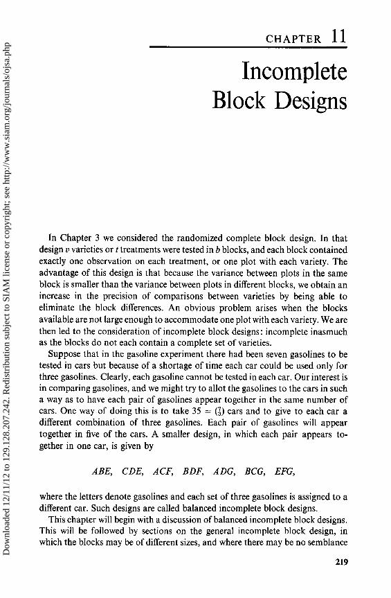
CHAPTER 11
IncompleteBlock Designs
In Chapter 3 we considered the randomized complete block design. In thatdesign v varieties or t treatments were tested in b blocks, and each block containedexactly one observation on each treatment, or one plot with each variety. Theadvantage of this design is that because the variance between plots in the sameblock is smaller than the variance between plots in different blocks, we obtain anincrease in the precision of comparisons between varieties by being able toeliminate the block differences. An obvious problem arises when the blocksavailable are not large enough to accommodate one plot with each variety. We arethen led to the consideration of incomplete block designs: incomplete inasmuchas the blocks do not each contain a complete set of varieties.
Suppose that in the gasoline experiment there had been seven gasolines to betested in cars but because of a shortage of time each car could be used only forthree gasolines. Clearly, each gasoline cannot be tested in each car. Our interest isin comparing gasolines, and we might try to allot the gasolines to the cars in sucha way as to have each pair of gasolines appear together in the same number ofcars. One way of doing this is to take 35 = ( 3) cars and to give to each car adifferent combination of three gasolines. Each pair of gasolines will appeartogether in five of the cars. A smaller design, in which each pair appears to-gether in one car, is given by
ABE, CDE, ACF, BDF, ADG, BCG, EFG,
where the letters denote gasolines and each set of three gasolines is assigned to adifferent car. Such designs are called balanced incomplete block designs.
This chapter will begin with a discussion of balanced incomplete block designs.This will be followed by sections on the general incomplete block design, inwhich the blocks may be of different sizes, and where there may be no semblance
219
Dow
nloa
ded
12/1
1/12
to 1
29.1
28.2
07.2
42. R
edis
trib
utio
n su
bjec
t to
SIA
M li
cens
e or
cop
yrig
ht; s
ee h
ttp://
ww
w.s
iam
.org
/jour
nals
/ojs
a.ph
p

220 Incomplete Block Designs [Ch. 11
of balance. We shall also discuss such topics as the recovery of interblockinformation. We have a choice of notations. We may talk either of t treatmentsor of v varieties. In this chapter we shall follow the more modern usage of talkingabout t treatments, although we shall still call the experimental units to whichthey are applied, plots. We shall thus have t treatments applied to several plots inb blocks. In the succeeding chapters we shall discuss partially balanced associa-tion schemes and the construction of incomplete block designs. In those chapterswe shall employ the older usage of v varieties because v is the usual notation inthat area.
11.1 Balanced Incomplete Block Designs
These designs were introduced by Yates (1936). They are designs for t treat-ments in b blocks. Each block contains k plots, k < t. Each plot contains asingle treatment and each treatment appears in r plots. We say that each treat-ment has r replications, or is replicated r times. No treatment appears more thanonce in any block. Each pair of treatments appears in the same block ,1 times.We shall sometimes use the abbreviations BIB design or BIBD.
The five parameters b, t, r, k, and A are not independent. They are integerssubject to the following restrictions:
(i) N = rt = bk, where N is the total number of plots;(ii) A(t — 1) = r(k — 1);
(iii) b >: t.
A design with b = t and r = k is raid to be symmetric.To establish restriction (ii) we consider any treatment, such as A. The treat-
ment A appears in r blocks, in each of which are also (k — 1) other treatments.There are, therefore, r(k — 1) plots, which are in the same block as a plotcontaining A. These plots have to contain the remaining (t — 1) treatmentsexactly \ times each. Hence, t(t — 1) = r(k — 1). The four parameter valuesb = 12, k = 4, t = 8, and r = 6 satisfy restrictions (i) and (iii). However,restriction (ii) gives A = 18/7, which is not an integer. Hence, there is nobalanced incomplete block design with those values of b, t, r, and k.
The incidence matrix of a design is the matrix N = ( n,) of t rows and bcolumns; nis is the number of times that the ith variety occurs in thejth block.For a balanced incomplete block design, n; is either one or zero, and n,2f = ni; .The matrix NN' has t rows and t columns. It is of considerable interest in thedevelopment of the theory of incomplete block designs. If we denote the elementsof NN' by q1 , we see that q{; = I f n2, and q;,, = L n,,nhf, (i 0 h). For thebalanced incomplete block design we have qi, = r and q,h = a, (i s4 h); we maytherefore write
NN' = (r — 2 )' + AJt,
Dow
nloa
ded
12/1
1/12
to 1
29.1
28.2
07.2
42. R
edis
trib
utio
n su
bjec
t to
SIA
M li
cens
e or
cop
yrig
ht; s
ee h
ttp://
ww
w.s
iam
.org
/jour
nals
/ojs
a.ph
p

Sec. 11.2] Some Balanced Incomplete Block Designs 221
where It is the identity matrix of order t and Jt is a square matrix of order t withevery element unity.
To evaluate the determinant of NN' we subtract the first column from each ofthe other columns, and then add all the other rows to the first row. It is nowreadily seen that
INN'l =(r—)t)t-1(r+(t— l)))=(r—A)t-lrk>0.
Thus NN' has rank t, and so N has rank t. However, N is a matrix of t rows andb columns so that r(N) < min(b, t). Hence, t < min(b, t), and the inequality(iii) is proved. This inequality is due to Fisher (1940). The proof that has beenpresented follows that of Bose (1949).
If the design is symmetric, b = t and N is square. In that case NN'I = ^Nl 2 ,and so (r — A)t - lr 2 is a perfect square. This implies that when t is even, (r — A)must be a square. Consider the set of parameters t = b = 22, r = k = 7, A = 2;t is even but r — A = 5, which is not a square, and so no design with theseparameters exists. This result [Shrikhande (1950)] shows that the conditionsgiven are necessary, but not sufficient, for the existence of a balanced incompleteblock design.
11.2 Some Balanced Incomplete Block Designs
For any pair of integers t, k(k < t), a balanced incomplete block design canbe obtained by taking all possible combinations of k out of t treatments. Forthese designs
b= (k)' r= (k— 1)' — (k-2).
There are, however, smaller designs for some values of t and k. The design givenat the beginning of the chapter with t = b = 7, r = k = 3, and 2. = 1 is anexample.
A design with t = 6, b = 10, r = 5, k = 3, and A = 2 is
ABE, ABF, ACD, ACF, ADE, BCD, BCE, BDF, CEF, DEF.
A design for t = 9, b = 12, r = 4, k = 3, and A = 1 can be obtained by usingorthogonal Latin squares. (The design is employed in the example in the nextsection.) A design with t = 16, b = 20, r = 5, k = 4, and A = 1 may beconstructed in a similar fashion. Both designs are from the orthogonal series ofYates. Their derivation will be discussed in Chapter 13. The second designfollows. We denote the treatments by 1, 2,..., 16. The treatments are written
Dow
nloa
ded
12/1
1/12
to 1
29.1
28.2
07.2
42. R
edis
trib
utio
n su
bjec
t to
SIA
M li
cens
e or
cop
yrig
ht; s
ee h
ttp://
ww
w.s
iam
.org
/jour
nals
/ojs
a.ph
p

222 Incomplete Block Designs [Ch. 11
in five 4 x 4 arrays and each array forms a complete replicate. The rows are theblocks.
I II III IV V
1 2 3 4 1 5 913 1 61116 1 71214 1 810155 6 7 8 2 6 10 14 2 5 12 15 2 8 11 13 2 7 9 169101112 3 7 11 15 3 8 914 3 51016 3 61213
13 14 15 16 4 8 12 16 4 7 10 13 4 6 9 15 4 5 11 14
This design has at least two applications outside the field of experimentaldesign. In each of the five groups of four blocks every treatment appears exactlyonce. The design may, therefore, be used in the following situation to allocatebridge players to tables. Suppose that sixteen bridge players are gathered to-gether for an evening and that there is enough time for five games to be played ateach table. How do we arrange the players so that each player plays five games;four tables are in continuous use and no player has to sit out for a time; andevery player has the opportunity to play one game at the same table as everyother player. The solution is to let replications correspond to games and treat-ments to players. Thus, during the fourth game of the evening the players at thefirst table are 1, 7, 12, and 14; at the second table they are 2, 8, 11, and 13, and soon.
The second application was found in Great Britain before the Second WorldWar in professional motorcycle racing on cinder tracks, a sport which is stillpopular there. The tracks are about 350 yards in circumference. Four riders takepart in each four-lap race, and an evening's program calls for about twentyraces. Usually the evening is devoted to team races between various teams in aleague, but occasionally the riders race as individuals. The following situationthen occurs. There are sixteen riders; they are to be arranged, four at a time, insuch a way that each rider races five times, and, during the evening, he races onceagainst each of the other fifteen men. This is achieved by using the balancedincomplete block design and letting treatments represent riders and blocksrepresent races. Unfortunately, the program cannot be arranged so that norider is obliged to ride in two consecutive races.
A design with t = 8, b = 14, r = 7, k = 4, and \ = 3 is obtained when a 23
design is repeated seven times in two blocks of four runs each time, confoundingin turn the three main effects and the four interactions. Writing, 1, 2, 3, 4, 5, 6,7, 8 for (1), a, b, ab, c, ac, bc, abc, respectively, the design is
1357 1256 1234 14582468 3478 5678 2367
1368 1278 14672457 3456 2358
Dow
nloa
ded
12/1
1/12
to 1
29.1
28.2
07.2
42. R
edis
trib
utio
n su
bjec
t to
SIA
M li
cens
e or
cop
yrig
ht; s
ee h
ttp://
ww
w.s
iam
.org
/jour
nals
/ojs
a.ph
p

Sec. 11.3] The Analysis of Balanced Incomplete Block Designs 223
The design that we have just given for t = 16 could be derived by addingd, ad, bd, ... = 9, 10, 11,.... Then the first replicate is obtained by dividing the24 factorial into four blocks, confounding C, D, CD. The effects confounded inthe other replicates are A, B, AB; AC, BD, ABCD; ABC, AD, BCD; BC, ABD,ACD.
The problems of the existence and construction of balanced incomplete blockdesigns have been of considerable interest to both statisticians and algebraists.(They will be the topic of Chapter 13.) The major paper on the construction ofdesigns is by Bose (1939). The Fisher and Yates tables contain a listing of almostall the known designs for r < 10 and k < 10. The restrictions on the parametershave led to the investigation of other types of incomplete block design, notablythe partially balanced incomplete block designs of Bose and Nair (1939); thesedesigns will be discussed in the next chapter.
11.3 The Analysis of Balanced Incomplete Block Designs
We consider now the usual method of analyzing balanced incomplete blockdesigns. This is called the intrablock analysis because the block differences areeliminated and the estimates of all contraets in the treatment effects can beexpressed in terms of comparisons between plots in the same block.
We have the following model:
ytf=µ+T{ +;3 +e L,,
where y,f is the observation, if there is one, on the ith treatment in the jth block,i-, is the effect of the ith treatment, fi, is the jth block effect, and ei, is the randomerror with the usual assumptions. The mean p and the treatment effects -rt areunknown constants. The block effects may be fixed or random; we treat them asif they are fixed. It is important to note that the model assumes that there is nointeraction between treatments and blocks.
The normal equations are
G=Nµ+r2f i +k,1$i, (11.1)
Ti = rµ + rfj + (11.2)
B1 = kµ + nijfj + kl^,, (11.3)
where Ti is the sum of all the observations on the ith treatment and B, is the sumof all the observations in the jth block.
Dow
nloa
ded
12/1
1/12
to 1
29.1
28.2
07.2
42. R
edis
trib
utio
n su
bjec
t to
SIA
M li
cens
e or
cop
yrig
ht; s
ee h
ttp://
ww
w.s
iam
.org
/jour
nals
/ojs
a.ph
p
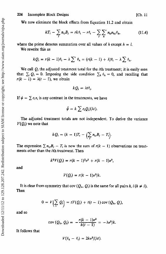
224 Incomplete Block Designs [Ch. 11
We now eliminate the block effects from Equation 11.2 and obtain
kTT — niiBf = rkfi — rfj — 1l'ntinhJfh , (11.4)1 1h
where the prime denotes summation over all values of h except h = i.We rewrite this as
kQt = r(k —l)fi —ArTh =(r(k-1)+,1)T{ — Alfh .
We call Q, the adjusted treatment total for the ith treatment; it is easily seenthat 1, Q, = 0. Imposing the side condition lh fh = 0, and recalling thatr(k — 1) = A(t — 1), we obtain
kQj = ^1tfi .
If 0 = 7 c,T, is any contrast in the treatments, we have
^ = k ctQil(At).
The adjusted treatment totals are not independent. To derive the varianceV(Qj) we note that
kQt =(k — 1)T,— (1n i,Bi —T,).i
The expression 1 nijBj — T, is now the sum of r(k — 1) observations on treat-ments other than the ith treatment. Then
k2 V(Q{) = r(k — 1)2a2 + r(k — 1)a2 ,
and
V(Q1) = r(k — 1)a2/k.
It is clear from symmetry that cov (Q,^, Q,) is the same for all pairs h, i (h 0 i).Then
0 = V(> Q {) = tV(Qi) + t(t — 1) cov (Qh, Q,),
and so
cov (Qh, Q^) _ —r(k — 1)o2
= —\a2/k.k(t — 1)
It follows that
V(fh — Tt) = 2ka2/(At).
Dow
nloa
ded
12/1
1/12
to 1
29.1
28.2
07.2
42. R
edis
trib
utio
n su
bjec
t to
SIA
M li
cens
e or
cop
yrig
ht; s
ee h
ttp://
ww
w.s
iam
.org
/jour
nals
/ojs
a.ph
p

Sec. 11.3] The Analysis of Balanced Incomplete Block Designs 225
Indeed, we may write the covariance matrix of the Q 1 as
cov Q = (AtI — AJ)a 2/k.
Then, writing 0 = c'T where r is the vector of treatment effects and c'1 =1'c = 0, we have
V(ç1) = ,1Z t2 V(c 'Q) = ^zt2 ' k c = ( ca)ka2 /( ,1t ) .
The analysis of variance table is slightly complicated by the fact that treat-ments are not orthogonal to blocks. We take the sum of squares for regressionµG + 1, TT T1 + I, B;p; and then subtract the sums of squares for the meanG 2IN (which we write as C), and for blocks (ignoring treatments), 2 Balk — C.The remainder is called the sum of squares for treatments (adjusted for blocks).We write it as St (aai). Then
St(u) = T1T4 + B,P, — 1 Bi/k + C.
But kB1P1 = Bi — kBfµ — Bi nS7 T1 , and so
st(aa1) _ (T1 — n11B5/k) Tf = Q1T, = k Q?/(\t).
TABLE 11.1ANALYSIS OF VARIANCE
Source SS d.f.
Total 1 1 y Jk — C N— 1Blocks (ignoring treatments) I BB lk — C b — 1Treatments (adjusted for
blocks) IQ1 = k Q?/(t) t — 1Residual By subtraction N — t — b + 1
The residual sum of squares is the sum of squares for intrablock error. In the Ftest for the hypothesis that all the treatment effects are zero, the mean square fortreatments (adj) is tested against the error mean square.
The efficiency of an incomplete block design in which each treatment appears rtimes is measured relative to the complete block design with the same number ofreplicates. For a complete block design with r observations on each treatment,V(Th — T1) = 2a2/r. If, for an incomplete block design, the average of the vari-ances of all contrasts (Th — T1) is 2a2/a, the efficiency of the design is defined tobe E = a/r.
For the balanced incomplete block designs we have a = At/k, so that E,1t/(rk). It is clear that for any design E < 1. Some authors write T 1 = Q1/rE and
Dow
nloa
ded
12/1
1/12
to 1
29.1
28.2
07.2
42. R
edis
trib
utio
n su
bjec
t to
SIA
M li
cens
e or
cop
yrig
ht; s
ee h
ttp://
ww
w.s
iam
.org
/jour
nals
/ojs
a.ph
p

226 Incomplete Block Designs [Ch. 11
St(BuJ) _ QZ/rE. That sum of squares is also called by some authors the sum ofsquares for treatments eliminating blocks.
Under the normality assumption the hypotheses -rh — ri = 0 may be tested bythe t test or by Tukey's method; Scheffé's S method may also be used for testingthe more complex contrasts.
EXAMPLE. The following data are taken from a dishwashing experiment[John (1961b)]. The treatments were detergents and the response observed wasthe number of plates washed under standard test conditions before the foamdisappeared. In the experiment, detergent solutions are made up and platessoiled with a standard soil are washed one at a time until they are clean. Thetesting procedure calls for three basins to be used (i.e., for three treatments to betested simultaneously), and the three operators wash at a common speed duringa test. A block is thus a set of three operators testing three detergents simultane-ously. We have t = 9, b = 12, r = 4, k = 3, and A = 1. The data and theanalysis of variance table follow. The letters denote treatments and the responsesare given in parentheses.
1. A (19) B(17) C(1l) 7. A (20) E(26) J (31)2. D (6) E (26) F (23) 8. B (16) F (23) G (21)3. G (21) H(19) J (28) 9. C (13) D (7) H(20)4. A (20) D (7) G (20) 10. A (20) F (24) H(19)5. B (17) E (26) H(19) 11. B (17) D (6) J (29)6. C (15) F (23) J (31) 12. C (14) E (24) G (21)
TABLE 11.2ANALYSIS OF VARIANCE
d.f. SS MS
Total 35 1512.75Blocks (unadjusted) 11 412.75 37.52Treatments (adjusted) 8 1086.81 135.85Residual 16 13.19 0.82
The adjusted treatment totals (Q, = 3T ;) are given by 3QA = 3, 3QB = — 20,3Q,=-56, 3QD =- 116, 3QE =53, 3QF =32, 3QG =15, 3QH =- 2,and 3Q,=91.
11.4 Resolvable Designs
An incomplete block design in which each treatment appears r times is said tobe resolvable if the blocks can be divided into r groups in such a way that eachgroup consists of a complete replication of the treatments, i.e., each group ofblocks contains each treatment exactly once. The designs for t = 8 and t = 16,
Dow
nloa
ded
12/1
1/12
to 1
29.1
28.2
07.2
42. R
edis
trib
utio
n su
bjec
t to
SIA
M li
cens
e or
cop
yrig
ht; s
ee h
ttp://
ww
w.s
iam
.org
/jour
nals
/ojs
a.ph
p

Sec. 11.5] The General Incomplete Block Design 227
given earlier, and the design for t = 9, used in the example, are all resolvabledesigns. Bose (1942c) showed that the following condition is necessary for abalanced incomplete block design to be resolvable:
b>— t +r-1.
If b = t + r — 1, the design is said to be affine resolvable. Bose's condition canbe derived from the weaker assumption that t is a multiple of k. It was sub-sequently derived from this assumption by Roy (1952), Mikhail (1960), andMurty (1961). We now give the proof by Murty.
Let t = nk where n is an integer, and b = nr. We have
r _ A _ r—) r— At-1 k-1 t—k k(n-1)
Then
r—.lr(n-1)rn—rb—rk t -1 t-1 t-1
But r-1=rk— t,1= k(r—nA), and so (r— a)/k=r—nA=(b—r)/(t — 1). All the parameters are integers, and so r — nA is an integer. Further-more, r > A, and so (r — ,1)/k > 0. It follows that (b — r) /(t — 1) > 1, and sob >— r + t — 1.
In the analysis of variance table for a resolvable design, the sum of squares forblocks (ignoring treatments) may be divided into a sum for replicates and a sumfor blocks in replicates.
11.5 The General Incomplete Block Design
The balanced incomplete block design is a special case of the general in-complete design; in the Jatter the blocks need not be of the same size, nor needeach treatment appear the same number of times. We shall stils consider ttreatments in b blocks. Suppose that the i th treatment is tested in ri plots and thatthe jth block contains k; plots, (ri , k; > 0); we do not need to assume thatkf < t for any or all j. As before, Ti denotes the total of all observations on theith treatment; B ; is the sum of all the observations in the jth block; T, B are thecorresponding vectors of treatment and block totals.
We define two matrices, R and K; R is a t x t matrix with diagonal elementsr1 , r2, ..., rt ; the off-diagonal elements are zero. We write this as R = diag(r1 , r2i ... , rt). The matrix K is defined as K = diag(k l , k2 , ... , kb). The incidentematrix of a design has already been defined as N = (n i,) where n ij is the numberof times that the ith treatment appears in the jth block. If nij = 0 or 1 for allpairs, the design is said to be binary. If k. = k for all j, the design is called
Dow
nloa
ded
12/1
1/12
to 1
29.1
28.2
07.2
42. R
edis
trib
utio
n su
bjec
t to
SIA
M li
cens
e or
cop
yrig
ht; s
ee h
ttp://
ww
w.s
iam
.org
/jour
nals
/ojs
a.ph
p

228 Incomplete Block Designs [Ch. 11
proper. If ri = r for all i, the design is called equireplicate. The most commonlyused designs are proper, binary, and equireplicate.
For all designs we have
Rl t = Nl,,, Klb = N'lt,
where 1,, denotes a vector of n unit elements. For a proper design, K = kI;for an equireplicate design, R = rI. Some authors let r and k denote the vectorsof ri and k,; they then write r° and kó for the matrices that we have called Rand K.
Let yifm denote the mth observation on the ith treatment in the jth block; for abinary design we omit the subscript m. The model is
Yijm = !L + Ti + Pi + eijm ,
where µ, Ti , and ,S are defined in the same way as they were for the balancedincomplete block design. We denote by T, (3, T, and the corresponding vectorsof effects and their estimates. For the present, Ti and ,8 are assumed to beunknown constante.
The normal equations are
G=N11+ rif,+ kj , ( 11.5)
Ti = riµ + r,f, + ni,ft> , i = 1, . .., t, (11.6)
Bf =kiµ+ nijf,+kfftf , j=1,...,b. (11.7)
Multiplying each equation of the set of equations (11.7) by the correspondingfraction ni;/k, for a given value of i and subtracting them all from the ithequation of the set (11.6) eliminates the block effects and µ, giving
Qi = Ti — nijBj/k> = rif, — 1 (1 niJnh5Iki) Th. (11.8)
In matrix notation the normal equations are
G N 1tR 16K %
T = Ri t R N T (11.9)
B K1b N' K
Multiplying both sides of the equation on the left by
[N - ' 0 0
F= 0 It —NK -1
0 —N'R -1 Ib
Dow
nloa
ded
12/1
1/12
to 1
29.1
28.2
07.2
42. R
edis
trib
utio
n su
bjec
t to
SIA
M li
cens
e or
cop
yrig
ht; s
ee h
ttp://
ww
w.s
iam
.org
/jour
nals
/ojs
a.ph
p
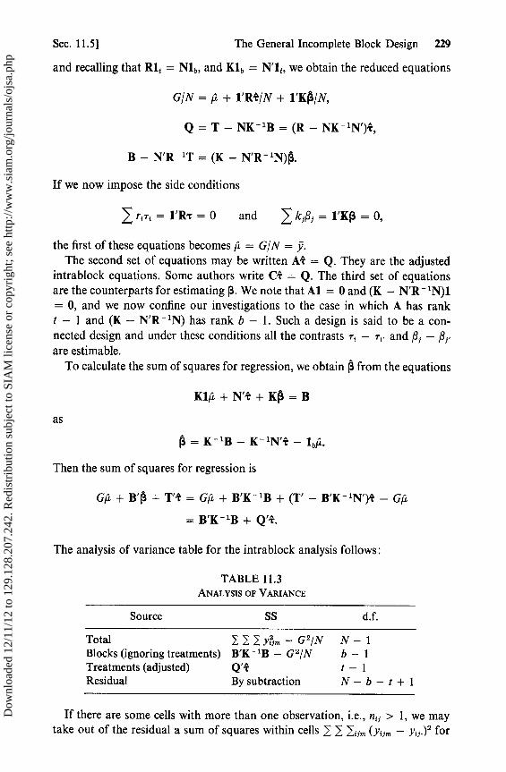
Sec. 11.5] The General Incomplete Block Design 229
and recalling that Rl t = Nl b, and Kl b = N'l t , we obtain the reduced equations
G/N = µ + 1'R' /N + 1'K/N,
Q=T—NK -1B=(R—NK -
B — N'R -1T = (K — N'R - 'N).
If we now impose the side conditions
r.i- = 1'RT = 0 and 1 kjpj = 1'Kp = 0,
the first of these equations becomes % = G/N = y.The second set of equations may be written AT = Q. They are the adjusted
intrablock equations. Some authors write CT = Q. The third set of equationsare the counterparts for estimating P. We note that Al = 0 and (K — N'R -1N)1= 0, and we now confine our investigations to the case in which A has rankt — 1 and (K — N'R - 'N) has rank b — 1. Such a design is said to be a con-nected design and under these conditions all the contrasts T l — Tt . and P; — P; .are estimable.
To calculate the sum of squares for regression, we obtain from the equations
K1µ+N'T+K = B
as
^ =K -1B—K - 'N 'T - 1bµ .
Then the sum of squares for regression is
Gµ+B' +T'T=Gµ+B'K -1B+(T'—B'K - 'N')T—Gµ
= B'K - 'B + Q'T.
The analysis of variance table for the intrablock analysis follows:
TABLE 11.3ANALYSIS OF VARIANCE
Source SS d.f.
Total 1 1 1 y jm — G ZIN N1Blocks (ignoring treatments) B'K - 1B — G 2/N b — 1Treatments (adjusted) Q'R t — 1Residual By subtraction N — b — t + 1
If there are some cells with more than one observation, i.e., n t5 > 1, we maytake out of the residual a sum of squares within cells 11 tijm (Yiim — y;5.) 2 for
Dow
nloa
ded
12/1
1/12
to 1
29.1
28.2
07.2
42. R
edis
trib
utio
n su
bjec
t to
SIA
M li
cens
e or
cop
yrig
ht; s
ee h
ttp://
ww
w.s
iam
.org
/jour
nals
/ojs
a.ph
p
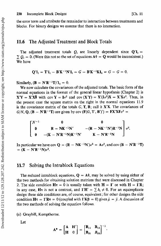
230 Incomplete Block Designs [Ch. 11
the error term and attribute the remainder to interaction between treatments andblocks. For binary designs we assume that there is no interaction.
11.6 The Adjusted Treatment and Block Totals
The adjusted treatment totals Q. are linearly dependent since Q'l t =1 Q{ = 0. (Were this not so the set of equations At = Q would be inconsistent.)We have
Q'1 t = T'1 t — B'K - 'N'1 t = G— B'K - 'Klb = G—G=0.
Similarly, (B — N'R -1T)'l b = 0.We now calculate the covariances of the adjusted totals. The basic form of the
normal equations in the format of the general linear hypothesis (Chapter 2) isX'Y = X'XO with cov Y = Iu2 and cov (X'Y) = X'(Ia 2)X = X'Xo2 . Thus, inthe present case the square matrix on the right in the normal equations 11.9is the covariance matrix of the totals G, T, B; call it X'X. The covariances ofG/N, Q, (B — N'R -1T) are given by cov (F(G, T', B')') = FX'XFa2 =
N -10 0
0 R — NK - 'N' —(R — NK - 1 N')R - 'N a2 .
0 —(K — N'R -1N)K -1N' K — N'R -1N
In particular we have cov Q = (R — NK - 'N')a2 = Ao2 , and cov (B — N'R - 'T)= (K — N'R - 1N)a2 .
11.7 Solving the Intrablock Equations
The reduced intrablock equations, Q = AT, may be solved by using either ofthe two methods for obtaining solution matrices that were discussed in Chapter2. The side condition H' = 0 is usually taken with H = 1' or with H = 1'R;in any case, H'r is not a contrast, and 1'H' = 1 h, 0. For an equireplicatedesign these side conditions are, of course, equivalent; for other designs the sidecondition H'r = 1'R r = 0 (coupled with 1'Kr3 = 0) gives µ = y. A discussion ofthe two methods of solving the equation follows.
(a) Graybill, Kempthorne.
LetA H' B12l
A*— [H 0 J [B„B21 B221
Dow
nloa
ded
12/1
1/12
to 1
29.1
28.2
07.2
42. R
edis
trib
utio
n su
bjec
t to
SIA
M li
cens
e or
cop
yrig
ht; s
ee h
ttp://
ww
w.s
iam
.org
/jour
nals
/ojs
a.ph
p
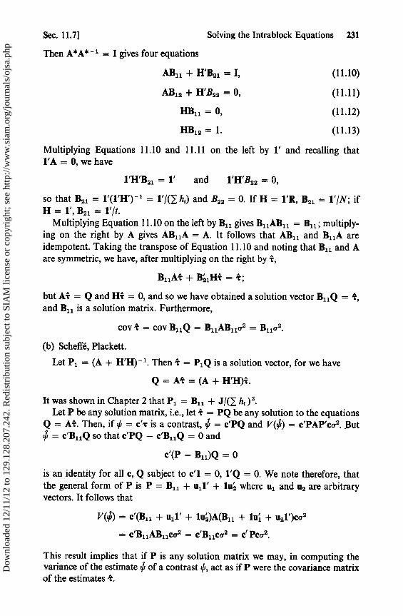
Sec. 11.7] Solving the Intrablock Equations 231
Then A*A* - I = I gives four equations
AB„ + H'B21 = I, (11.10)
ABia + H'B22 = 0, (11.11)
HB11 = 0, (11.12)
HB12 = 1• (11.13)
Multiplying Equations 11.10 and 11.11 on the left by 1' and recalling that1'A = 0, we have
1'H'B21 = 1' and 1'H'B22 = 0,
so that B21 = 1'(l'H') 1 = 1'/(1 h,) and B22 = 0. If H = 1'R, B21 = 1'/N; ifH = 1', B2 = 1'/t.
Multiplying Equation 11.10 on the left by B 11 gives B11AB11 = B11; multiply-ing on the right by A gives AB 11A = A. It follows that AB„ and B 11A areidempotent. Taking the transpose of Equation 11.10 and noting that B 11 and Aare symmetric, we have, after multiplying on the right by T,
B11AT + Bá1HR = T;
but AR = Q and HT = 0, and so we have obtained a solution vector B11Q = T,and B11 is a solution matrix. Furthermore,
cov T = cov B11Q = B11AB11a 2 = B11a2 .
(b) Scheffé, Plackett.
Let Pl = (A + H'H) -1 . Then T = P1Q is a solution vector, for we have
Q=A4=(A+H'H)T.
It was shown in Chapter 2 that P l = B11 + J/(1 h1) 2.Let P be any solution matrix, i.e., let T = PQ be any solution to the equations
Q = AT. Then, if 0 = c',r is a contrast, = c'PQ and V(^) = c'PAP'ca 2. But= c'B11Q so that c'PQ — c'B 11Q = 0 and
c'(P — B11)Q = 0
is an identity for all c, Q subject to c'1 = 0, 1'Q = 0. We note therefore, thatthe general form of P is P = B11 + ul l' + 1uá where ul and u2 are arbitraryvectors. It follows that
V(^) = c'(B11 + u1 1' + 1uá)A(B l1 + lui + u21')ca2
= c 'B11AB11ca2 = c 'Bl1ca2 = c Pca2 .
This result implies that if P is any solution matrix we may, in computing thevariance of the estimate + of a contrast 0, act as if P were the covariance matrixof the estimates R.
Dow
nloa
ded
12/1
1/12
to 1
29.1
28.2
07.2
42. R
edis
trib
utio
n su
bjec
t to
SIA
M li
cens
e or
cop
yrig
ht; s
ee h
ttp://
ww
w.s
iam
.org
/jour
nals
/ojs
a.ph
p
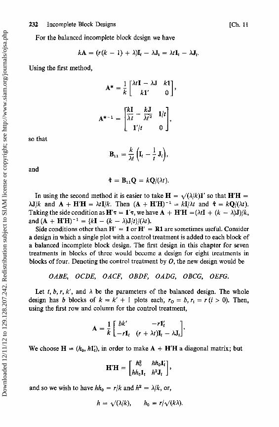
232 Incomplete Block Designs
[Ch. 11
For the balanced incomplete block design we have
kA = (r(k — 1) + A)It — ^Jt = AtI, — ^Jt .
Using the first method,
A* — 1 — AJ kl[AtI
kl' 0],
kI —
kJ 1/tA* -1 = í`t í
1'It 0so that
Bll = at (I` — t J`)'and
T = B11Q = kQ/(at).
In using the second method it is easier to take H = \/(A/k)1' so that H'H =AJ/k and A + H'H = AtI/k. Then (A + H'H) -1 = k1/,1t and t = kQ/(At).Taking the side condition as H',r = 1'T, we have A + H'H = (AtI + (k — ^1)J)lk,and (A + H'H) -1 = {kI — (k — ^1)J/t}/(,1t).
Side conditions other than H' = 1 or H' = Rl are sometimes useful. Considera design in which a single plot with a control treatment is added to each block ofa balanced incomplete block design. The first design in this chapter for seventreatments in blocks of three would become a design for eight treatments inblocks of four. Denoting the control treatment by 0, the new design would be
OABE, OCDE, OACF, OBDF, OADG, OBCG, OEFG.
Let t, b, r, k', and A be the parameters of the balanced design. The wholedesign has b blocks of k = k' + 1 plots each, ro = b, ri = r (i > 0). Then,using the first row and column for the control treatment,
_1 bk' —r1A [—rl t (r + ,1t)It — 1Jt1
We choose H = (ho , hlt), in order to make A + H'H a diagonal matrix; but
hó hhol 1^H'H = f hho lt h2 Jt
and so we wish to have hho = r/k and h2 = A/k, or,
h = 1/(Â/k), ho = rI1^(ka).
Dow
nloa
ded
12/1
1/12
to 1
29.1
28.2
07.2
42. R
edis
trib
utio
n su
bjec
t to
SIA
M li
cens
e or
cop
yrig
ht; s
ee h
ttp://
ww
w.s
iam
.org
/jour
nals
/ojs
a.ph
p

Sec. 11.9] The Recovery of Interblock Information 233
With this choice of H we have
1 +r2/A 0[bk'
0 ( + At)It]A +HM
'
whence
kAQ0 kQ,-0 _ r(r + At) , T__i r + At
(l > O).
11.8 Connected Designs
The idea of connected designs is due to Bose. A block and a treatment are saidto be associated if the treatment appears in the block. Two treatments, A and B,are said to be connected if we can form a chain of treatments and blocks:treatment—block—treatment—block— • • • —treatment, beginning with A andending with B, such that every block in the chain is associated with both thetreatments adjacent to it. The relationship A connected to B is an equivalencerelation which forms disjoint equivalence classes for the treatments. A design issaid to be connected if there is only one equivalence class, i.e., if every pair oftreatments is connected.
The following design for four blocks I, II, III, IV and seven treatments isconnected:
I ABCD, II BCE, III DE, IV EFG.
A and G are connected by the chain A—I—B—II—E—IV—G. Denoting theeffects of A, B,. . . , by T l , r2i ... , we see that r 1 — -r7 is estimable. We follow thechain and consider the contrast
Z = Yl l - Y21 + Y22 - Y52 + Y54 - Y74 ;
E(z) = T1 + N1 - T2 - N1 + T2 + N2 - T5 - N2 + T5 + N4 - T7 - N4
= T 1 - T7-
The following design with t = b = 6, which is the union of two disjointdesigns having no treatment in common, is disconnected:
AB, AC, BC, DE, DF, EF.
11.9 The Recovery of Interblock Information
Yates (1940) pointed out that under certain circumstances a second set ofestimates of the treatment effects, called the interblock estimates, can be obtained.
Dow
nloa
ded
12/1
1/12
to 1
29.1
28.2
07.2
42. R
edis
trib
utio
n su
bjec
t to
SIA
M li
cens
e or
cop
yrig
ht; s
ee h
ttp://
ww
w.s
iam
.org
/jour
nals
/ojs
a.ph
p
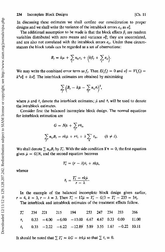
234 Incomplete Block Designs [Ch. 11
In discussing these estimates we shall confine our consideration to properdesigns and we shall write the variance of the intrablock errors e ;J as Qé.
The additional assumption to be made is that the block effects ,J are randomvariables distributed with zero means and variance ab; they are uncorrelated,and are also not correlated with the intrablock errors e ;J . Under these circum-stances the block totals can be regarded as a set of observations:
BJ = kp + nijrt + (kf3 + ^ e15).
We may write the combined error term as fJ . Then E(J) = 0 and af = V(f,) _
k2oó + ka'. The interblock estimates are obtained by minimizing
(BJ — kµ —
where ji and T I denote the interblock estimates; µ and Tf will be used to denotethe intrablock estimates.
Consider first the balanced incomplete block design. The normal equationsfor interblock estimation are
G=Nµ+^rTt ,
n, JB, = rkµ + rT{ + A 7" Th , (h # i ).J
We shall denote 1 ni5BJ by T. With the side condition 1'r = 0, the first equationgives µ = G/N, and the second equation becomes
Ti' = (r — a)T{ + rkµ,
whence
Ti — rkµT _, r—A
In the example of the balanced incomplete block design given earlier,r=4,k=3,r—A=3.ThenTi — 1212=T1 —G/3=T, —233=3f1 .
The interblock and intrablock estimates of the treatment effects follow.
T, 234 221 215 194 253 247 234 233 266
0.33 —4.00 —6.00 —13.00 6.67 4.67 0.33 0.00 11.00
Ti 0.33 —2.22 —6.22 —12.89 5.89 3.55 1.67 —0.22 10.11
It should be noted that 1 Ti = kG = trkµ so that T, = 0.
Dow
nloa
ded
12/1
1/12
to 1
29.1
28.2
07.2
42. R
edis
trib
utio
n su
bjec
t to
SIA
M li
cens
e or
cop
yrig
ht; s
ee h
ttp://
ww
w.s
iam
.org
/jour
nals
/ojs
a.ph
p
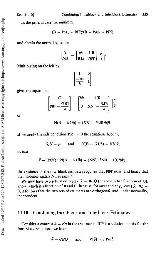
Sec. 11.10] Combining Intrablock and Interblock Estimates 235
In the general case, we minimize
(B — kµ1 6 — N'T)'(B — kµ1 6 — N'T)
and obtain the normal equations
INB, — Rlk NN'] [T]
Multiplying on the left by
1 0
—R1 1
b
gives the equations
G bk 1'R
NB— Gb1 0 NN' — RJR [:1
or
N(B — G 1/b) = (NN' — RJR/b)T.
If we apply the side condition 1'R'r = 0 the equations become
G/N = µ and N(B — G1/b) = NN',
so that
T = (NN') - 'N(B — G1/b) _ (NN') - 'NB — 1(G/bk);
the existence of the interblock estimates requires that NN' exist, and hence thatthe incidence matrix N has rank t.
We now have two sets of estimates: T = B 11 Q (or some other function of Q),and T, which is a function of B and G. Because, for any i and any j, cov (Q ; , B.) =0, it follows that the two sets of estimates are orthogonal, and, under normality,independent.
11.10 Combining Intrablock and Interblock Estimates
Consider a contrast 0 = c'T in the treatments. If P is a solution matrix for theintrablock equations, we have
= c'PQ and V(^) = c'Pcaé.
Dow
nloa
ded
12/1
1/12
to 1
29.1
28.2
07.2
42. R
edis
trib
utio
n su
bjec
t to
SIA
M li
cens
e or
cop
yrig
ht; s
ee h
ttp://
ww
w.s
iam
.org
/jour
nals
/ojs
a.ph
p

236 Incomplete Block Designs [Ch. 11
The interblock estimate of ¢ is
= c'T = c'(NN') -1NB;
the term G 1/b drops out because 0 is a contrast and V(^) = c'(NN') - 'ca'.We now wish to combine these two uncorrelated estimates of 0 to obtain an
unbiased joint estimate with minimum variance. We shall use the followingwell-known property of combined estimates.
Let 0 and 02 be unbiased estimates of a parameter 0 with variances v l and v2
and zero covariance. Consider the class of combined estimates of the formu1 01 + u2 02. In this class the minimum variance unbiased estimate of 0 is(w1B1 + w202)/(wi + w2) where the weights are wl = vi l and w2 = v2 1 ; i.e.,the individual estimates 0 and 02 are given weights inversely proportional totheir variances.
In the present case we should take for the combined estimate of + s,
0* = (w + w2G)/(w1 + w2),
where wl = 1 /c'Pco and w2 = 1 /c'(NN') lcaf. This simplifies to
* _ cV() + cV(^)V(0) + V(+)
If we knew vé and af, we could now obtain &*. The original method of Yatesfor the balanced incomplete block design is to use this weighted estimate, butwith the weights computed by substituting for oé and a estimates obtained fromthe data. Rao (1947a) derived combined estimates under the assumption that thee 5 and the P are normally distributed. For the balanced incomplete block designthe methods of Yates and of Rao give the same estimates. Rao's derivation willbe given later in this chapter.
We shall now confine our discussion to the case of balanced incomplete blockdesigns. In that case, P = kI/(At) and V(^) = c'ckaé/(At). For the interblockestimates, NN' = (r — A)I, + and
(NN ,) _ 1 = I — I — ^1Jr—d (r—A)(r+(t-1)d) r—A1 (r—A)rk'
but c'J = 0, and so we have
_ c'NB _ ciTi ' V c'ca2r—a r—,1 ()—r—A
The minimum variance joint estimate is thus
0* = (w14 + w2)/(w1 + w2),
Dow
nloa
ded
12/1
1/12
to 1
29.1
28.2
07.2
42. R
edis
trib
utio
n su
bjec
t to
SIA
M li
cens
e or
cop
yrig
ht; s
ee h
ttp://
ww
w.s
iam
.org
/jour
nals
/ojs
a.ph
p
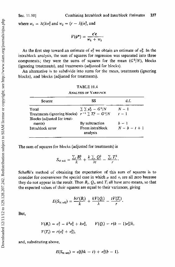
Sec. 11.101 Combining Intrablock and Interblock Estimates 237
where wl = At/kaé and wz = (r — A)/o, and
V(b*) = c c .wl + w2
As the first step toward an estimate of of we obtain an estimate of ab. In theintrablock analysis, the sum of squares for regression was separated into threecomponents; they were the sums of squares for the mean (G 2/N), blocks(ignoring treatments), and treatments (adjusted for blocks).
An alternative is to subdivide into sums for the mean, treatments (ignoringblocks), and blocks (adjusted for treatments).
TABLE 11.4ANALYSIS OF VARIANCE
Source SS d.f.
Total 1 1 y g — G 2/N N — 1Treatments (ignoring blocks) r' 1 T{ — G 2/N t — 1Blocks (adjusted for treat-
ments) By subtraction b — 1Intrablock error From intrablock N — b — t + 1
analysis
The sum of squares for blocks (adjusted for treatments) is
2
ilbl adJ = Ij B1 + k Gí Q? — Jt T2S .
k Al r
Scheffé's method of obtaining the expectation of this sum of squares is toconsider for convenience the special case in which µ and -r, are all zero becausethey do not appear in the result. Then B;, Qi , and T, all have zero means, so thatthe expected values of their squares are equal to their variances, giving
E(S„ au) = bV(B,)
+ kV(Qti) _ tV(Ti)
k a r
But,
V(B5) = af = k2ab + ka, V(Q) = r(k — 1)oé/k,
V (T=) = r (ab + tee),
and, substituting above,
E(Sbi aaJ) = ab(bk — t) + aé(b — 1).
Dow
nloa
ded
12/1
1/12
to 1
29.1
28.2
07.2
42. R
edis
trib
utio
n su
bjec
t to
SIA
M li
cens
e or
cop
yrig
ht; s
ee h
ttp://
ww
w.s
iam
.org
/jour
nals
/ojs
a.ph
p
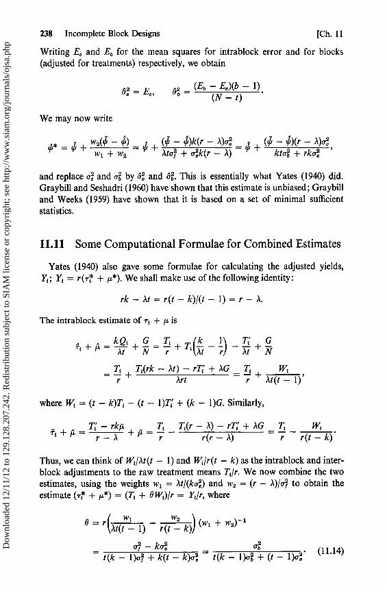
238 Incomplete Block Designs [Ch. 11
Writing EQ and Eb for the mean squares for intrablock error and for blocks(adjusted for treatments) respectively, we obtain
Qé = Eei &2 = (En — Ee)(b — 1) .
(N — t)
We may now write
+/!* _ +^ + ww(+ ) + At f + )a k(r ^) i4
) (r )teA)
__ + ( ktv + rkó
and replace oé and ab by $' and Q6. This is essentially what Yates (1940) did.Graybill and Seshadri (1960) have shown that this estimate is unbiased; Graybilland Weeks (1959) have shown that it is based on a set of minimal sufficientstatistics.
11.11 Some Computational Formulae for Combined Estimates
Yates (1940) also gave some formulae for calculating the adjusted yields,Y,; Y, = r(r? + µ*). We shall make use of the following identity:
rk— At= r(t—k)/(t— 1)=r—A.
The intrablock estimate of r, + µ is
kQ 1 GTi(xt-
11T1 GT` +µ At + N r +T` rl At + N
T1 + T,(rk—At)—rT1 +AGTi + Wi
r Art r At(t — 1) ,
where Wi = (t — k)Ti — (t — 1)T{ + (k — 1)G. Similarly,
_ T11 —rkµ _ TiT1(r—A)—rTi+AGTi W{Tt+µ r—A i7_ r(r—A) r r(t—k)
Thus, we can think of W/At(t — 1) and Wi/r(t — k) as the intrablock and inter-block adjustments to the raw treatment means T{/r. We now combine the twoestimates, using the weights w l = At/(ka) and w2 = (r — A)/of to obtain theestimate (T* + µ*) = (Ti + 9W)/r = Y,/r, where
B — r (At(t 1 1) — r(tw? k)) (wl + w2) -1
=af — kaé ob
= t(k — 1)a2 + k(t — k)oé t(k — 1)ab + (t — 1)o2(11.14)
Dow
nloa
ded
12/1
1/12
to 1
29.1
28.2
07.2
42. R
edis
trib
utio
n su
bjec
t to
SIA
M li
cens
e or
cop
yrig
ht; s
ee h
ttp://
ww
w.s
iam
.org
/jour
nals
/ojs
a.ph
p

Sec. 11.11 ] Some Computational Formulae for Combined Estimates 239
We may rearrange Equation 11.14 and obtain
of = k(1 + (t — k)0)oé/(1 — t(k — 1)9),
and, after some further algebraic manipulation,
V(S*) = c'c(wl + w2) - ' = c'c(l + (t — k)B)o /r.
When Eb is large by comparison to Ee we have, taking the limit as Eb 00,0 = l/{t(k — 1)}; then (1 + (t — k)B)oé/r becomes koé/(at), which gives thevariance of the intrablock estimator.
Substituting &, &b for oe, ob as before, we have
__ (Eb—Ee)(b-1)B t(k — 1)(b — 1)(Eb — Ee) + (N — t)(t — 1)Ee
(Eb — Ee)(b — 1)t(k — 1)(b — l)Eb + (t — k)(b — t)Ee
For the symmetric design with b = t, 0 takes the simpler form
9=Eb —EQ/t(k-1)Eb .
If Eb < Ee , it is usual to take 0 = 0. This is equivalent to putting Eb = Ee in theformula and to acting as if there were no block effects; thus the design is analyzedas a completely randomized design.
Yates also considered the situation in which the blocks can be broken up intoc groups of bie blocks each, each group consisting of r/c complete replicationsof the treatments; r/c is an integer. Although Equation 11.14 still holds, theestimate of ob is changed. We return to Scheffé's method of calculation and add aterm for the sum of squares between groups in the analysis of variance table.Let G„ denote the group total for the gth group. Then
Bf Gg k Q, _ T{2 G 2Sb' 8a^ — k k — f N/c + At r + N
Assuming that r,, g are all zero, and also that there is no group effect,
V(G9) = bV(Bj)/c and V(G) = bV(B,),
where V(B5) = of. Then
E(Sbl ") = k V(Q{) — r V(Ti) + b(b — c + 1)
V(B)N
= (k(b — c + 1) — t)ab + (b — c)oé f
so that
ob = (Eb — EQ)(b — c)/{N — t — k(c — 1)}.
Dow
nloa
ded
12/1
1/12
to 1
29.1
28.2
07.2
42. R
edis
trib
utio
n su
bjec
t to
SIA
M li
cens
e or
cop
yrig
ht; s
ee h
ttp://
ww
w.s
iam
.org
/jour
nals
/ojs
a.ph
p

240 Incomplete Block Designs [Ch. 11
If the design is resolvable, the blocks can be arranged to form single replicates.In this case, c = r, and the previous result simplifies to
ob = (Eb — EQ)r/{k(r — 1)}.
Substituting in Equation 11.14, we obtain for the general case
__ (Eb — Ee)(b — c)B t(k— 1)(b—c)Eb +(t—k)(b—c—t+ 1
and, for the resolvable case,
(Eb—Ee)re rt(k— 1)Eb +k(b—r—t+ 1)Ee
A special case is the balanced lattice. This is the balanced design with t = k2 ,
r = k + 1, and b = k(k + 1). We have already seen examples for t = 9 andt = 16. In this case, the formula is further simplified to
8 = (Eb — Ee)Ik 2(k — 1)Eb .
EXAMPLE. James and Bancroft (1951) carried out a 2 3 experiment in abalanced incomplete block design. They took clover plants, split them into twohalves, and applied a different treatment combination to each half. A block is apair of half plants. The response observed was the percentage of hard leed; theyconsidered using the arcsine transformation on the data, but decided against it.The treatments in the design were the 2 3 treatment combinations in a factorialexperiment, with factors calcium (C), phosphorus (P), and potassium (K). Thetreatments represented by A, B,. . . , H are, respectively, (1), k, p, pk, c, ck, cp,cpk. The design is resolvable and the data are arranged in seven replications;the parameters of the design are t = 8, b = 28, r = 7, k = 2. and A = 1.
I II III IV
A 38 B 29 A 37 C 27 A 15 D 23 A 3 E 13C 49 D 28 B 37 H 50 B 47 G 64 B 45 C 36E 32 F 29 D 90 E 89 C 35 F 39 D 11 G 24G 64 H 32 F 28 G 71 E 22 H 18 F 39 H 37
V VI VII
A 23 F 39 A 66 G 68 A 28 H 30B21 D 14 B 23 F 46 B 10 E 40C 18 H 10 C 22 E 28 C 32 G 33E 23 G 53 D 23 H 39 D 18 F 23D
ownl
oade
d 12
/11/
12 to
129
.128
.207
.242
. Red
istr
ibut
ion
subj
ect t
o SI
AM
lice
nse
or c
opyr
ight
; see
http
://w
ww
.sia
m.o
rg/jo
urna
ls/o
jsa.
php
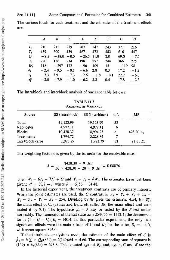
Sec. 11.11 ] Some Computational Formulae for Combined Estimates 241
The various totals for each treatment and the estimates of the treatment effectsare
A B C D E F G H
T, 210 212 219 207 247 243 377 216Tt 439 500 439 467 472 482 616 447Q, -9.5 -38.0 -0.5 -26.5 11.0 2.0 69.0 -7.5Y, 220 186 234 198 257 244 366 225
W, 118 -297 172 - 96 109 15 -119 98 -2.4 -9.5 -0.1 -6.6 2.8 0.5 17.2 -1.9
Tt -7.3 2.9 -7.3 -2.6 -1.8 -0.1 22.2 -6.0T* -3.0 -7.9 -1.0 -6.2 2.2 0.4 17.8 -2.3
The intrablock and interblock analysis of variance table follows:
TABLE 11.5ANALYSIS OF VARIANCE
Source SS (Intrablock) SS (Interblock) d.f. MS
Total 19,123.99 19,123.99 55Replicates 4,977.11 4,977.11 6Blocks 10,428.37 8,994.25 21 428.30 Eb
Treatments 1,794.72 3,228.84 7Intrablock error 1,923.79 1,923.79 21 91.61 EQ
The weighting factor 0 is given by the formula for the resolvable case:
_ 7(428.30 - 91.61)B 56 x 428.30 + 28 x 91.61 = 0.08876.
Then W, = 6Ti - 7T1 + G and Yt = Ti + 0W. The estimates have just beengiven; T* = Y1/7 - µ where µ = G/56 = 34.48.
In the factoraal experiment, the treatment contrasts are of primary interest.When the joint estimates are used, the C contrast is Y5 + Y6 + Y, + Y8 -
Y, - Y2 - Y3 - Y4 = 254. Dividing by 8r gives the estimate, 4.54, for P*,the main effect of C. (James and Bancroft called 2 1 the main effect and esti-mated it by 9.1). The hypotheses /3 = 0 may be tested by the F test undernormality. The numerator of the test statistic is 2542/56 = 1152.1; the denomina-tor is (1 + (t - k)0)EQ = 140.4. In this particular experiment, the only twosignificant effects were the main effects of C and K; for the latter, Bk = - 4.0,
with mean square 896.0.
If the intrablock analysis is used, the estimate of the main effect of C is= k 1 ± Q 1/(8At) = 2(149)/64 = 4.66. The corresponding sum of squares is
(149) x k/(8)t) = 693.8. This is tested against Eef and, again, C and K are the
Dow
nloa
ded
12/1
1/12
to 1
29.1
28.2
07.2
42. R
edis
trib
utio
n su
bjec
t to
SIA
M li
cens
e or
cop
yrig
ht; s
ee h
ttp://
ww
w.s
iam
.org
/jour
nals
/ojs
a.ph
p

242 Incomplete Block Designs [Ch. 11
only two significant effects. The sums of squares for the several contraets add upto the sum of squares for treatments, adjusted for blocks. They are
C P K CP CK PK CFK1152.1 240.3 896.0 73.1 126.0 301.8 283.5
11.12 Other Combined Estimates
In previous sections the estimate of ab was obtained from Eb . This is not theonly method. Yates (1940) subdivided the sum of squares for blocks ignoringtreatments into a treatments component and a remainder. The interblockestimates, T, were obtained by least squares analysis from the set of b observa-tions Bi. The total sum of squares 1, B1 — G/b was then divided into twocomponents: regression, l { TtT,, and remainder, with t — 1 and b — t d.f.,respectively. The remainder has expectation (b — t)af. The total is Sbl ig trmultiplied by k. Hence, dividing each of the component sums of squares by k, wehave a subdivision of Sb l ig tr into a treatment component li Ti T,/k and aremainder. The mean square of the Jatter component is an unbiased estimate of'af/k with (b — t) degrees of freedom.
The ten different sums of squares that have been considered during thisdiscussion of balanced incomplete block designs are collected in table 11.6,together with their expectations, under the assumptions that treatments arefixed with the side condition 1, Ti = 0 and that blocks are random. Undernormality they have, with the proper divisors, chi-square distributions, and theF test can be used to test hypotheses, r = 0, and ab = 0.
S1 , S2 , S3 , S6, and S9 appear in the intrablock analysis and are distributedindependently under normality. S 4 and 55 are independent of S l , 52, S6, and Sa
under normality. S1 , S2i S7 , S8 , and 59 appear in the interblock analysis andare independent under normality.
Graybill and Deal (1959) use as their combined estimator (T 1 + BW)/r, with0 given by (11.14) and Qé and ab estimated by Ee and S5/(b — t). By an argumentthat depends heavily upon the assumption of normality, they show that whenthe flf are normally distributed their estimator is unbiased and is uniformlybetter than either or l in the sense that V(i*) < min (V(#), V(^)) for allvalues of oé and ab when b >_ t+ 10 or when b= t+9 and N — b — t+1 >_ 18. Seshadri (1963a,b) also discusses alternate combined estimates of thistype.
11.13 Maximum Likelihood Estimation
We now consider the maximum likelihood method under normality, given byRao (1947a). We shall assume in the derivation that we have a general incompleteblock design, the only restriction being that it is proper; it does not have to be
Dow
nloa
ded
12/1
1/12
to 1
29.1
28.2
07.2
42. R
edis
trib
utio
n su
bjec
t to
SIA
M li
cens
e or
cop
yrig
ht; s
ee h
ttp://
ww
w.s
iam
.org
/jour
nals
/ojs
a.ph
p

Sou
rce
SS
TA
BL
E11
.6A
NA
LY
SIS
OF
VA
RIA
NC
E d.f.
ESS
e
80
Raw
tota
l8
1M
ean
82
Tot
al8
3B
lock
s(u
nad
just
ed)
divi
ded
into
84
Tre
atm
ent
com
po
nen
t8
5R
emai
nd
er8
6T
reat
men
ts(a
djus
ted)
87
Tre
atm
ents
(una
djus
ted)
88
Blo
cks
(adj
uste
d)8
9In
trab
lock
erro
r
Y'y
G2
/N8
0-
81
k-
1L
BJ-
81
[LT
?/k
(r-
A)]
-[8
1rk/(r
-A
)]8
3-
84
kQ
'Q/A
tr:!
LT?
-8
1
S3+
86
-8
7
82
-8
3-
86
=8
2-
87
-8
6
N 1 N-
1
b-
11
-1
b-
1
1-
11
-1
b-
1N
-b
-I+
l
NfL
2+
Na~
+r
Lorr
+Na~
NfL
2+
a~
+ka~
(N-
l)a~
+r
Lorr
+(N
-k)a~
(b-
l)a~
+(r
-A
)L
-rN
k+
(N-
k)ag
(t-
l)a~
+(r
-A
)L
-rN
k+
ttk
-k)
ag(b
-I)a~
+(N
-Ik)a~
=(b
-I)a~/k
(I-
l)a~
+A
tL
-rN
k(I
-l)a~
+r
L-r~
+(I
-k)
ag(b
-l)a~
+(N
-I)a~
(N-
b-
1+
l)a~
Dow
nloa
ded
12/1
1/12
to 1
29.1
28.2
07.2
42. R
edis
trib
utio
n su
bjec
t to
SIA
M li
cens
e or
cop
yrig
ht; s
ee h
ttp://
ww
w.s
iam
.org
/jour
nals
/ojs
a.ph
p
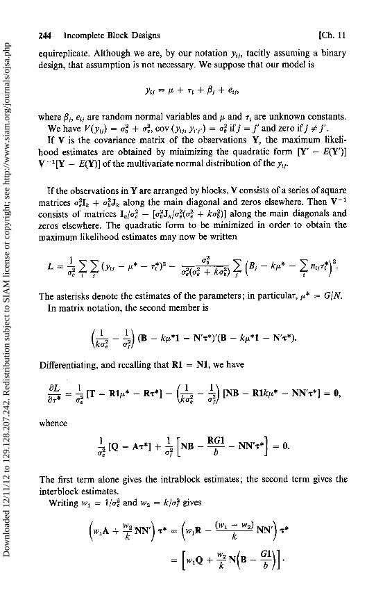
244 Incomplete Block Designs [Ch. 11
equireplicate. Although we are, by our notation p ij, tacitly assuming a binarydesign, that assumption is not necessary. We suppose that our model is
yir= !L+T, +flr+etr,
where P;, e{; are random normal variables and µ and Tl are unknown constants.We have V(y) = ob + oé, cov (yt;, yt -;•) = ab ifj = j' and zero ifj j'.If V is the covariance matrix of the observations Y, the maximum likeli-
hood estimates are obtained by minimizing the quadratic form [Y' — E(Y')]
V -1 [Y — E(Y)] of the multivariate normal distribution of the y.
If the observations in Y are arranged by blocks, V consists of a series of squarematrices a Ik + abJk along the main diagonal and zeros elsewhere. Then V'consists of matrices Ik/al — [abJk /oé(Qe + kab)] along the main diagonals andzeros elsewhere. The quadratic form to be minimized in order to obtain themaximum likelihood estimates may now be written
L = 11(y,r — µ* — T*)2 — oe(Qé f kab) (B' — kµ* — ntiT)2•
The asterisks denote the estimates of the parameters; in particular, µ* = G/N.
In matrix notation, the second member is
( 1 2 1)
2 (B — kµ*1 — N'T*)'(B — kµ*1 — N'*).
Differentiating,
\, e ar
Differentiating, and recalling that Rl = Nl, we have
8r = Qé [T — R1µ* — RT*] — (Fa
é — of) [NB — Rlkµ* — NN'r*] = 0,
whence
Qé[Q—As*]+Qf [NB— Rb1 —NN',r*] =0.
The first term alone gives the intrablock estimates; the second term gives theinterblock estimates.
Writing wl = 1 /vé and w2 = k/v? gives
(w1A + k NN') T* = (w,R — (w1 k w2) NN') T*
[w,Q + k N `B b111
Dow
nloa
ded
12/1
1/12
to 1
29.1
28.2
07.2
42. R
edis
trib
utio
n su
bjec
t to
SIA
M li
cens
e or
cop
yrig
ht; s
ee h
ttp://
ww
w.s
iam
.org
/jour
nals
/ojs
a.ph
p

Sec. 11.14] The General Balanced Design 245
The individual equations may be written
Pi = Ri 1 T* — Ah{T h
k h#t k
where, for binary designs,
Pi = Wi Qi + k (1 nijB; — w(riG/ b))
Ri = ri(wi + w2/(k — 1 )), Aht = Ahi(wl — w2),
and >hi = 1 nhjnij• For a binary design, Ahi is the number of times that the hthand ith treatments appear in the same block. The combined estimates can thusbe obtained by substituting P i , R, and A, for Q, ri , and 'h in the solutions tothe intrablock equations. As before, we substitute for aé and ab estimates fromthe intrablock and interblock analyses of variance.
For the balanced incomplete block design, the methods of Yates and of Raogive the same combined estimates. This is not, however, true in the general case[see Sprott (1956a)]. It should be noted that the use of Rao's method does notrequire that the matrix NN' be of full rank. We shall use this method in thenext chapter for the simple lattice design in which n 2 treatments are tested in adesign with k = n, b = 2n, and r = 2, in this case, b < t.
11.14 The General Balanced Design
A general incomplete block design is said to be balanced if, with T = 0, inthe intrablock analysis, V(Th — Ti) is the same for all pairs of treatments h and i,h 0 i. Atiqullah (1961) showed that this implied that if the covariance matrix ofthe estimates is Vol, the diagonal elements of V are all equal and the off-diagonal elements are all equal.
Solving the normal equations by the first method with H = 1', we havecov 4 = B11a2 so that V = B„ and Vl = B11 1 = 0. Denote the elements of Vby Vht . Then, if the design is balanced,
1J(Th — Ti) = (Vhh + vtt — 2vht)a2 = da2
for all pairs h, i, where d is some constant. Summing over all i, 1 < i < t, wehave
(t — 1)d = (t — l)vhh + r ' vii — 2 r / vht,
where the prime denotes summation over all i, except i = h. However, sinceVl = 0, li vhi = 0, and the equation becomes
(t — 1)d = tv,^h + tr (V),
Dow
nloa
ded
12/1
1/12
to 1
29.1
28.2
07.2
42. R
edis
trib
utio
n su
bjec
t to
SIA
M li
cens
e or
cop
yrig
ht; s
ee h
ttp://
ww
w.s
iam
.org
/jour
nals
/ojs
a.ph
p
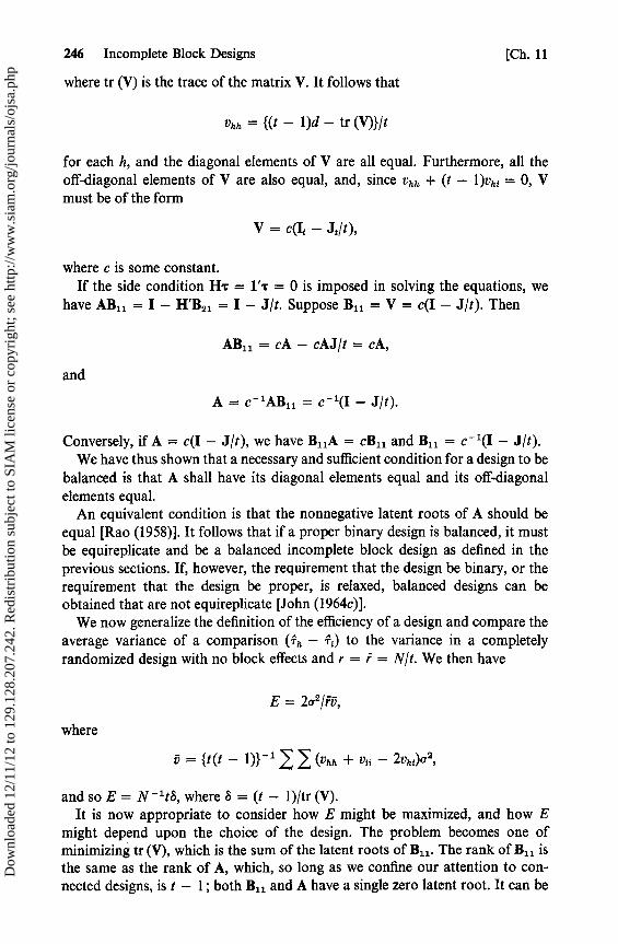
246 Incomplete Block Designs [Ch. 11
where tr (V) is the trace of the matrix V. It follows that
v,,h = {(t — 1)d — tr (V)}/t
for each h, and the diagonal elements of V are all equal. Furthermore, all theoff-diagonal elements of V are also equal, and, since vhh + (t — l)Vhi = 0, Vmust be of the form
V = c(It — Je/t),
where c is some constant.If the side condition Hr = 1'T = 0 is imposed in solving the equations, we
have AB„ = I — H'B21 = I — J/t. Suppose B 11 = V = c(I — J/t). Then
AB„ = cA — cAJ/t = cA,
and
A = c -1AB11 = c -1(I — J/t).
Conversely, if A = c(I — J/t), we have B11A = cBll and B11 = c -1(I — J /t).We have thus shown that a necessary and sufficient condition for a design to be
balanced is that A shall have its diagonal elements equal and its off diagonalelements equal.
An equivalent condition is that the nonnegative latent roots of A should beequal [Rao (1958)]. It follows that if a proper binary design is balanced, it mustbe equireplicate and be a balanced incomplete block design as defined in theprevious sections. If, however, the requirement that the design be binary, or therequirement that the design be proper, is relaxed, balanced designs can beobtained that are not equireplicate [John (1964c)].
We now generalize the definition of the efficiency of a design and compare theaverage variance of a comparison (Th - Ti) to the variance in a completelyrandomized design with no block effects and r = r = N/t. We then have
E = 2a2/rv,
where
v = { t(t — 1)} - 11(vhn + vti — 2vnt)Q2,
and so E = N -1 t8, where 8 = (t — 1)/tr (V).It is now appropriate to consider how E might be maximized, and how E
might depend upon the choice of the design. The problem becomes one ofminimizing tr (V), which is the sum of the latent roots of B 11 . The rank of B11 isthe same as the rank of A, which, so long as we confine our attention to con-nected designs, is t — 1; both B11 and A have a single zero latent root. It can be
Dow
nloa
ded
12/1
1/12
to 1
29.1
28.2
07.2
42. R
edis
trib
utio
n su
bjec
t to
SIA
M li
cens
e or
cop
yrig
ht; s
ee h
ttp://
ww
w.s
iam
.org
/jour
nals
/ojs
a.ph
p
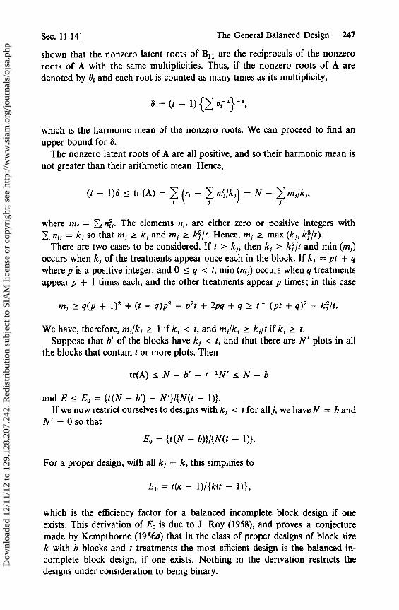
Sec. 11.14] The General Balanced Design 247
shown that the nonzero latent roots of B 11 are the reciprocals of the nonzeroroots of A with the same multiplicities. Thus, if the nonzero roots of A aredenoted by 0i and each root is counted as many times as its multiplicity,
= (t — 1) { or '} - ',
which is the harmonic mean of the nonzero roots. We can proceed to find anupper bound for 8.
The nonzero latent roots of A are all positive, and so their harmonic mean isnot greater than their arithmetic mean. Hence,
(t — 1)S < tr (A) _ (r, — > n?/k;) = N — mf/k; ,
where mf = ^; n. The elements n15 are either zero or positive integers withl i n,f = k; so that mf >_ kf and mf >t kf /t. Hence, m; >— max (k; , k2 /t).
There are two cases to be considered. If t >t k;, then kf >t kf /t and min (m,)occurs when k; of the treatments appear once each in the block. If kf = pt + qwhere p is a positive integer, and 0 < q < t, min (m5) occurs when q treatmentsappear p + 1 times each, and the other treatments appear p times; in this case
mi ? q(p + 1 )2 + (t — q)p 2 = p2t + 2pq + q > t -1(pt + q)2 = k;/t.
We have, therefore, mi/k >_ 1 if kf < t, and m1/k5 >_ kj/t if k! >_ t.Suppose that b' of the blocks have k; < t, and that there are N' plots in all
the blocks that contain t or more plots. Then
tr(A)<N—b'—t - 'N'<N—b
and E < Eo = {t(N — b') — N'}/{N(t — 1)}.If we now restrict ourselves to designs with kf < t for all j, we have b' = b and
N' = 0 so that
Eo = {t(N — b)}/{N(t — 1)}.
For a proper design, with all ki = k, this simplifies to
Eo = t(k — 1)/{k(t — 1)},
which is the efficiency factor for a balanced incomplete block design if oneexists. This derivation of Eo is due to J. Roy (1958), and proves a conjecturemade by Kempthorne (1956a) that in the class of proper designs of block sizek with b blocks and t treatments the most efficient design is the balanced in-complete block design, if' one exists. Nothing in the derivation restricts thedesigns under consideration to being binary.
Dow
nloa
ded
12/1
1/12
to 1
29.1
28.2
07.2
42. R
edis
trib
utio
n su
bjec
t to
SIA
M li
cens
e or
cop
yrig
ht; s
ee h
ttp://
ww
w.s
iam
.org
/jour
nals
/ojs
a.ph
p
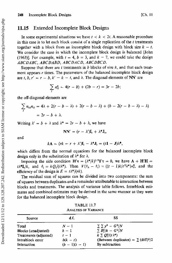
248 Incomplete Block Designs [Ch. 11
11.15 Extended Incomplete Block Designs
In some experimental situations we have t < k < 2t. A reasonable procedurein this case is to let each block consist of a single replication of the t treatmentstogether with a block from an incomplete block design with block size k — t.We consider the case in which the incomplete block design is balanced [John(1963)]. For example, with t = 4, b = 3, and k = 7, we could take the designABCDABC,ABCDABD,ABCDACD,ABCDBCD.
Suppose that there are t treatments in b blocks of size k, and that each treat-ment appears r times. The parameters of the balanced incomplete block designare t, b, r' = r — b, k' = k — t, and A. The diagonal elements of NN' are
^nt = 4(r — b) + (2b — r) = 3r — 2b;
the off-diagonal elements are
flhj ij =4A+ 2(r — b — A) + 2(r — b — A) + (b — 2(r — b — A) — A)
=2r—b+A.
Writing A' = b + A and A* = 2r — b + t, we have
NN' = (r — ')It + A*J t ,
andkA= (rk —r+'\')It — ^1*Jt =(tI—J)A*,
which differs from the normai equations for the balanced incomplete blockdesign only in the substitution of )* for A.
Imposing the side condition H'T = (A*/k) 1121'T = 0, we have A + H'H =tA*It/k, and 1 = kQ i/(t.k*). Then V(Th, - Ti) = {(t — 1)k/t 2 A*}oé, and theefficiency of the design is E = t,1*/(rk).
The residual sum of squares can be divided into two components: the sumof squares between duplicates and a remainder attributable to interaction betweenblocks and treatments. The analysis of variance table follows. Interblock esti-mates and combined estimates may be derived in the same manner as they werefor the balanced incomplete block design.
TABLE 11.7ANALYSIS OF VARIANCE
Source d.f. SS
Total N— 1 1 y2 — GZINBlocks (unadjusted) b — 1 Bj lk — G 2 f NTreatments (adjusted) t — 1 k 7- Q;/(t ) *)
Intrablock error b(k — t) (Between duplicates) _ (diff) 2/2Interaction (b — 1)(t — 1) By subtractionD
ownl
oade
d 12
/11/
12 to
129
.128
.207
.242
. Red
istr
ibut
ion
subj
ect t
o SI
AM
lice
nse
or c
opyr
ight
; see
http
://w
ww
.sia
m.o
rg/jo
urna
ls/o
jsa.
php

Exercises 249
Exercises
1. Is the equation
E(Sm aai) = a (bk — t) + oé(b — 1)
true for any binary, proper, equireplicate design? Is it true if any of the threerestrictions, binary, proper, and equireplicate, are removed?
2. A design for two treatments has p pairs of blocks. Each block has three plots.In each pair one block has two plots with A and one with B, and the other has twoplots with B and a single plot with A. Analyze the design. How would your analysisbe modified if p = mq, and the p pairs are actually m pairs at each level of afactor with q levels?
3. Apply the methods of this chapter to the case of a randomized complete blockdesign in which the first treatment is missing from the first block.
4. In a resolvable balanced incomplete block design consider the first block in thefirst replication. Let m,j denote the number of treatments that this block has incommon with the jth block of the !th replication (1 < i <_ r, 1 < j < b/r).Show that the average of the m,j is m = k2 /v, and that their variance is given by
(m,j — m)2 = k(t — k)(b — t — r + 1)/{n2(r — 1)(t — 1)},15
where n = tik. For an affine resolvable design mt, = m for all i, j [Bose (1 942c)].5. Find the combined estimates for the extended block design, Sec. 11.15.
Dow
nloa
ded
12/1
1/12
to 1
29.1
28.2
07.2
42. R
edis
trib
utio
n su
bjec
t to
SIA
M li
cens
e or
cop
yrig
ht; s
ee h
ttp://
ww
w.s
iam
.org
/jour
nals
/ojs
a.ph
p

CHAPTER 12
Partially BalancedIncomplete
Block Designs
Much of our emphasis in the last chapter was upon balanced incomplete blockdesigns. Unfortunately, such designs do not exist for all combinations ofparameters that we might wish to use. In particular, the requirement that A be aninteger imposes a severe restriction upon the number of treatments for whichbalanced designs of a reasonable size can be found. It will be recalled that if thereare t treatments each repeated r timer in blocks of size k, then A = r(k — 1)1(t — 1). If (t — 1) is a prime, r has to be a multiple of (t — 1), and then there isthe further restriction that b = rt/k has to be an integer. For example, if t = 32,r must be a multiple of 31; if, in addition, k is odd, and thus prime to 32, b hasto be a multiple of 31 x 32.
The characteristic property of a balanced incomplete block design is thatV(fh - fi) has the same value for all pairs, h, i, of treatments. An alternative torequiring balance is to find a design in which the condition of equal variances ismodified somewhat. This can be achieved by the use of partially balanceddesigns. In a partially balanced design with two associate classes, V(fh — fl)may take either of two values, depending upon whether the hth and ith treat-ments are first or second associates of each other. When there are m associateclasses, V(Th - f,) may take any of m values.
Partially balanced incomplete block designs (PBIB designs) were introducedby Bose and Nair (1939). Their idea has been developed considerably since then,largely by Bose and his students. In 1952 Bose and Shimamoto introduced theconcept of partially balanced association schemes and the definition of apartially balanced design was rephrased in terms of this concept. We shall usethe definition given by Bose (1963) in a review paper.
The symbol v will be used to denote the number of treatments. This will
i^,j1l
Dow
nloa
ded
12/1
1/12
to 1
29.1
28.2
07.2
42. R
edis
trib
utio
n su
bjec
t to
SIA
M li
cens
e or
cop
yrig
ht; s
ee h
ttp://
ww
w.s
iam
.org
/jour
nals
/ojs
a.ph
p
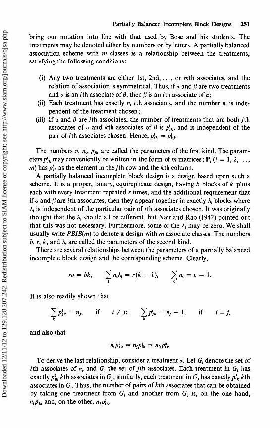
Partially Balanced Incomplete Block Designs 251
bring our notation into line with that used by Bose and his students. Thetreatments may be denoted either by numbers or by letters. A partially balancedassociation scheme with m classes is a relationship between the treatments,satisfying the following conditions:
(i) Any two treatments are either 1st, 2nd, ..., or mth associates, and therelation of association is symmetrical. Thus, if a and P are two treatmentsand a is an ith associate of P, then P is an ith associate of a;
(ii) Each treatment has exactly n t ith associates, and the number n { is inde-pendent of the treatment chosen;
(iii) If a and P are ith associates, the number of treatments that are both jthassociates of a and kth associates of Pis p, and is independent of thepair of ith associates chosen. Hence, plk = pki.
The numbers v, ni , Pk are called the parameters of the first kind. The param-eters P ik may conveniently be written in the form of m matrices; Pi (i = 1, 2,...,m) has Pik as the element in the jth row and the kth column.
A partially balanced incomplete block design is a design based upon such ascheme. It is a proper, binary, equireplicate design, having b blocks of k plotseach with every treatment repeated r times, and the additional requirement thatif a and P are i th associates, then they appear together in exactly t. blocks where,1t is independent of the particular pair of ith associates chosen. It was originallythought that the A l should all be different, but Nair and Rao (1942) pointed outthat this was not necessary. Furthermore, lome of the Â. may be zero. We shallusually write PBIB(m) to denote a design with m associate classes. The numbersb, r, k, and A, are called the parameters of the second kind.
There are several relationships between the parameters of a partially balancedincomplete block design and the corresponding scheme. Clearly,
rv=bk, >n jA =r(k— l), ^ni =v— 1.
It is also readily shown that
Pik = n1 , if ij; Pk = nj — 1, if i =j,k k
and also that
niP`ik = nJP+fk = nkP r
To derive the last relationship, consider a treatment a. Let G { denote the set ofith associates of a, and Gi the set of jth associates. Each treatment in G i hasexactly pfk kth associates in G1 ; similarly, each treatment in Gf has exactlyp'k kthassociates in G. Thus, the number of pairs of kth associates that can be obtainedby taking one treatment from G i and another from G; is, on the one hand,n,p 1k and, on the other, njpik.
Dow
nloa
ded
12/1
1/12
to 1
29.1
28.2
07.2
42. R
edis
trib
utio
n su
bjec
t to
SIA
M li
cens
e or
cop
yrig
ht; s
ee h
ttp://
ww
w.s
iam
.org
/jour
nals
/ojs
a.ph
p

252 Partially Balanced Incomplete Block Designs [Ch. 12
Most of the research carried out so far has been concerned with designs havingtwo associate classes. Chapter 14 will be devoted to the construction of designsfrom association schemes. Bose and Shimamoto (1952) classified all the knownPBIB(2) designs into five types. Simple designs are those for which either Al orA, = 0. The other designs correspond to one of the following four associationschemes: group divisible, triangular, Latin square, and cyclic. Extensivecollections of designs are given by Bose and Shimamoto (1952), and by Bose,Clatworthy, and Shrikhande (1954). For m = 2, the relationships between theparameters just given take the simpler form:
n 1 +n2 =v— 1, n1A1 + n2 A2 = r(k — 1),
Pij + p12 = nl — 1, P21 + Pz2 = n2,
Pi + P12 = ni, P21 + PL = n2 — 1,
niP12 = n2Pii, n1P22 = n2P12.
12.1 The Group Divisible Association Scheme
This is a scheme for v = mn treatments where m and n are integers. Thetreatments are divided into m groups of n treatments each. Treatments in thesame group are first associates; treatments in different groups are secondassociates. This corresponds to writing the v symbols for the treatments in arectangular array of m rows and n columns, and letting the rows be the groups.For this scheme v = mn, nl = n — 1, and n2 = n(m — 1),
n -2 0 0 n-1Pl = [ 0 n(m —1 )]' P2 = [n —1 n(m — 2),
It can be shown that a necessary and sufficient condition for a PBIB(2) associa-tion scheme to be group divisible is that p1 2 (or P12) = 0. It is customary toabbreviate group divisible to GD.
As an example of a GD design, consider the following design for v = 6:
1,2,3; 3,4,5; 2,5,6; 1,2,4; 3,4,6; 1,5,6.
The three groups are 1 and 2, 3 and 4, 5 and 6. We have Al = 2, X12 = 1.We shall show in Chapter 14 that the following inequalities hold for all GD
designs:
r>_Al, rk—A2v>-0.
Bose and Connor (1952) have divided the GD designs into three classes:
(i) Singular designs having r = A l ;(ii) Semiregular designs having r > d l and rk = A2v;
(iii) Regular designs having r > Al and rk > Azv.
Dow
nloa
ded
12/1
1/12
to 1
29.1
28.2
07.2
42. R
edis
trib
utio
n su
bjec
t to
SIA
M li
cens
e or
cop
yrig
ht; s
ee h
ttp://
ww
w.s
iam
.org
/jour
nals
/ojs
a.ph
p

Sec. 12.2] Intrablock Analysis of GD Designs 253
A trivial example of a singular design is obtained by letting each row of therectangular array constitute a block.
12.2 Intrablock Analysis of GD Designs
The intrablock equations for a GD design are easily solved. In Chapter 11 wederived the intrablock equations, Q = A-?, for the general incomplete blockdesign. The reduced equation for .the hth treatment is
Qh = nhfTh — nhiniifil k.
Writing S1(h) = 1s (TS) where the summation is made over all the first associatesof the hth treatment and defining S2(fh) similarly for the second associates,we have
kQh = r(k — l)fh — 1S1(h) — A2SI(fh)
_ {r(k — 1) + 1}Th — À1{Th + S1(Th)} — A2S2(rh)•
Suppose now that the treatments are labeled in order so that treatments 1through n form the first group, treatments n + 1 through 2n form the secondgroup, and so on. The matrix A then consists of square submatrices
{r(k — 1) + k1}In — A1J.n
along the main diagonal and submatrices —1\2Jn off the diagonal. We take theside condition 1 Ti = 0 in the form HT = 0 where H = hl and h 2 = A2/k.Then k(A + H'H) consists of square matrices {r(k — 1) + Al}I„ + (a2 — ,11)Jn
along the diagonal and zero elsewhere. The solution matrix (A + H'H) -1
thus consists of submatrices
k_ (,12 — A l)Jr(k— 1)+j[I {r(k— 1) +A1 +nA2 —nal},
k 1 LI (A2 —v Al)
JJr(k-1) +a a
along the main diagonal and zero elsewhere.It follows that
{r(k — 1) + A }f = kQh — k(\2 — 'Al){Qh + Sl(Qh)}/(vA2)
where Sj(Qh) is the sum 1$ Q$ for all the first associates of the hth treatment.
Dow
nloa
ded
12/1
1/12
to 1
29.1
28.2
07.2
42. R
edis
trib
utio
n su
bjec
t to
SIA
M li
cens
e or
cop
yrig
ht; s
ee h
ttp://
ww
w.s
iam
.org
/jour
nals
/ojs
a.ph
p
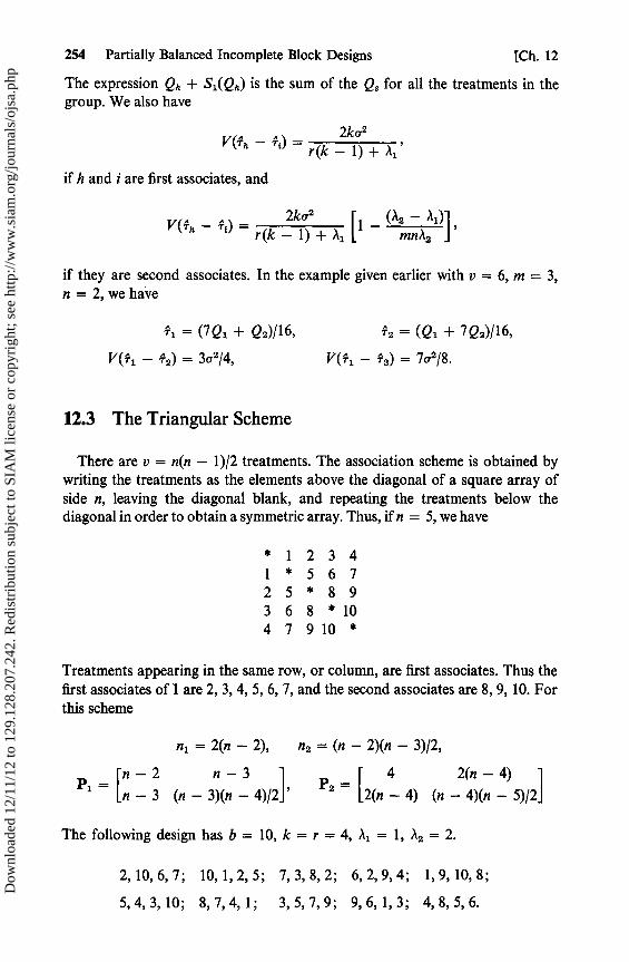
254 Partially Balanced Incomplete Block Designs [Ch. 12
The expression Qh + S(Q) is the sum of the Q. for all the treatments in thegroup. We also have
2ka2V(Th-T()= r(k- 1)+Al
'
if h and i are first associates, and
2ka2
i r(A2 — á i)1
V(Th—Ti)=r(k-1)+,1 1_
mnJ J'
if they are second associates. In the example given earlier with v = 6, m = 3,n = 2, we have
T^ = (7 Q1 + Q2)/ 16 ,
V(T1 - T2) = 3a2 /4,
T2 = (Qi + 7Q 2)/16,
V(T1 - T3) = 702 '8.
12.3 The Triangular Scheme
There are v = n(n — 1)/2 treatments. The association scheme is obtained bywriting the treatments as the elements above the diagonal of a square array ofside n, leaving the diagonal blank, and repeating the treatments below thediagonal in order to obtain a symmetric array. Thus, if n = 5, we have
* 1 2 3 41 * 5 6 72 5 * 8 93 6 8 * 104 7 9 10 *
Treatments appearing in the same row, or column, are first associates. Thus thefirst associates of 1 are 2, 3, 4, 5, 6, 7, and the second associates are 8, 9, 10. Forthis scheme
nl = 2(n — 2), n2 = (n — 2)(n — 3)/2,
_ n-2 n-3 _ 4 2(n-4)Pl— [n-3 (n-3)(n-4)/2,' PZ— [2(n-4) (n-4)(n-5)/2]
The following design has b = 10, k = r = 4, dl = 1, A2 = 2.
2,10,6,7; 10,1,2,5; 7,3,8,2; 6,2,9,4; 1,9,10,8;
5,4,3,10; 8,7,4,1; 3,5,7,9; 9,6,1,3; 4,8,5,6.
Dow
nloa
ded
12/1
1/12
to 1
29.1
28.2
07.2
42. R
edis
trib
utio
n su
bjec
t to
SIA
M li
cens
e or
cop
yrig
ht; s
ee h
ttp://
ww
w.s
iam
.org
/jour
nals
/ojs
a.ph
p
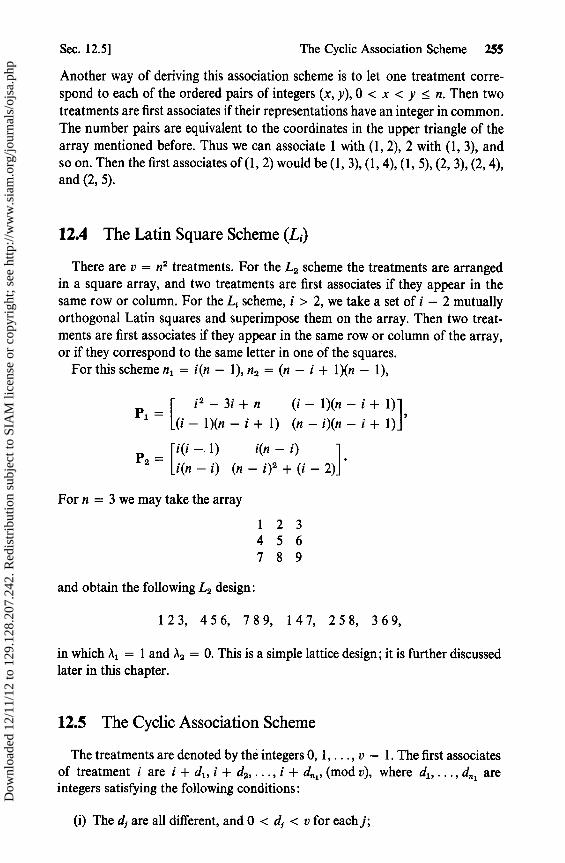
Sec. 12.5] The Cyclic Association Scheme 255
Another way of deriving this association scheme is to let one treatment corre-spond to each of the ordered pairs of integers (x, y), 0 < x <y < n. Then twotreatments are first associates if their representations have an integer in common.The number pairs are equivalent to the coordinates in the upper triangle of thearray mentioned before. Thus we can associate 1 with (1, 2), 2 with (1, 3), andso on. Then the first associates of (1, 2) would be (1, 3), (1, 4), (1, 5), (2, 3), (2, 4),and (2, 5).
12.4 The Latin Square Scheme (L i)
There are v = n 2 treatments. For the L2 scheme the treatments are arrangedin a square array, and two treatments are first associates if they appear in thesame row or column. For the L, scheme, i > 2, we take a set of i — 2 mutuallyorthogonal Latin squares and superimpose them on the array. Then two treat-ments are first associates if they appear in the same row or column of the array,or if they correspond to the same letter in one of the squares.
For this scheme n l = i(n — 1), n2 = (n — i + 1)(n — 1),
i 2 -3i+n (i— 1)(n—i+1)Pl
_— [(i— 1)(n—i+ 1) (n—i)(n—i+ 1)]^
P2
—. 1) i(n — i)
[
i«i(n—i) (n—i) 2 +(i-2)]^
For n = 3 we may take the array
1 2 34 5 67 8 9
and obtain the following L2 design:
123, 456, 789, 147, 258, 369,
in which i\ 1 and A2 = 0. This is a simple lattice design; it is further discussedlater in this chapter.
12.5 The Cyclic Association Scheme
The treatments are denoted by the integers 0, 1, ..., v — 1. The first associatesof treatment i are i + dl , i + d2i ..., i + d 1 , (mod v), where dl , ..., d,, 1 areintegers satisfying the following conditions:
(i) The di are all different, and 0 < d, < v for each j;
Dow
nloa
ded
12/1
1/12
to 1
29.1
28.2
07.2
42. R
edis
trib
utio
n su
bjec
t to
SIA
M li
cens
e or
cop
yrig
ht; s
ee h
ttp://
ww
w.s
iam
.org
/jour
nals
/ojs
a.ph
p
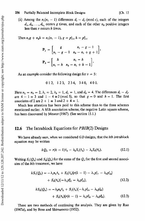
256 Partially Balanced Incomplete Block Designs [Ch. 12
(ii) Among the n l(nl — 1) differences d5 — d;- (mod v), each of the integersdl , d2,. . . , d„, occurs g times, and each of the other n2 positive integersless than v occurs h times.
Then n1g + n2h = n1(n1 — 1 ), g = Pil, h = P119
g n1—g-1P1 =
n1 —g-1 n2 —n1 +g+1
h nl — hP2 = nl —h n2 —n 1 +h-1
As an example consider the following design for v = 5:
012, 123, 234, 340, 401.
Here n 1 = n2 = 2, Al = 2, A2 = 1, dl = 1, and d2 = 4. The differences d1 — d5
are 4 — 1 = 3 and 1 — 4 - 2 (mod 5), so that g = 0 and h = 1. The firstassociates of 2 are 2 + 1 = 3 and 2 + 4 - 1.
Much less attention has been paid to this scheme than to the three schemesmentioned earlier. A fifth association scheme, the negative Latin square scheme,has been discovered by Mesner (1967). (See section 15.1.)
12.6 The Intrablock Equations for PBIB(2) Designs
We have already seen, when we considered GD designs, that the hth intrablockequation may be written
kQh = r(k — 1) h — 1S1( h) — A2S2(h). (12.1)
Writing Sl(Qh) and S2(Qh) for the sums of the QS for the first and second associ-ates of the hth treatment, we have
kSl(Qh) = — íiln1 ,, + S1(Th){r(k — 1) — A1P111 — A2P12}
+ S2(){— i\1Pi1 — ^2Pi2}, (12.2)
kS2(Qh) = — '2n2Th + Sl(Th){ — A1Pi2 — A2P122}
+ S2(Th){r(k — 1) — >'1P12 — "2P22}. (12.3)
There are two methods of continuing the analysis. They are given by Rao(1947a), and by Bose and Shimamoto (1952).
Dow
nloa
ded
12/1
1/12
to 1
29.1
28.2
07.2
42. R
edis
trib
utio
n su
bjec
t to
SIA
M li
cens
e or
cop
yrig
ht; s
ee h
ttp://
ww
w.s
iam
.org
/jour
nals
/ojs
a.ph
p
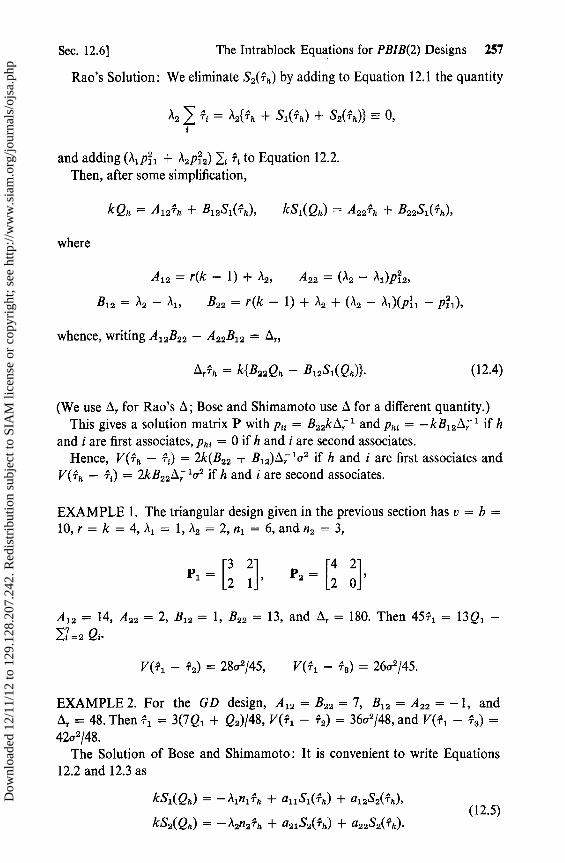
Sec. 12.6] The Intrablock Equations for PBIB(2) Designs 257
Rao's Solution: We eliminate S2(Th) by adding to Equation 12.1 the quantity
n2 T4 = '2{Th + S1(h) + J2(fh)} = 0,
and adding (aspil + A2p22) to Equation 12.2.
Then, after some simplification,
kQh = Al2Th + B12S1(fh), kSl(Qh) = A22Th + B22S1(Th),
where
Al2 = r(k — 1) + '2, A22 = (A2 — al)P125
B12 = A2 — A1, B22 = r(k — 1) + A 2 + ("2 — A1)(pil — Pil)
whence, writing Al2B22 — A22B12 = 0„
ArTh = k{B22Qh — B12S1(Qh)}• (12.4)
(We use A, for Rao's A; Bose and Shimamoto use A for a different quantity.)This gives a solution matrix P with p i; = B22kAr 1 and ph; _ —kB12 Ar 1 if h
and i are first associates, Phi = 0 if h and i are second associates.Hence, V(Th — T{) = 2k(B22 + B12)Or lv2 if h and i are first associates and
V(Th — Tt) = 2kB22 AT 1Q2 if h and i are second associates.
EXAMPLE 1. The triangular design given in the previous section has v = b =10, r = k = 4, A = 1, a2 = 2, n 1 = 6, and n2 =3,
P1 = [2 1]' P2 = [2 0]
A l2 = 14, A 22 = 2, B12 = 1, B22 = 13, and A, = 180. Then 45T 3 = 13Q 1 —
i=2 Qi.
V(T1 — T2) = 28a2/45, Y (T1 — f,) = 26a2/45.
EXAMPLE 2. For the GD design, Al2 = B22 = 7, B12 = A22 = — 1, andA, = 48. Then T l = 3(7Q1 + Q2)/48, V(T1 — T2) = 3602/48, and V(T1 — T3) _
4202/48.The Solution of Bose and Shimamoto: It is convenient to write Equations
12.2 and 12.3 as
kSl(Qh) = — Â 1n1 Th + allS1(Th) + a12S2(fh),
/ (12.5)kS2(Qh) = — A2n2Th + a21S2(Th) + a22S2(Th)•
Dow
nloa
ded
12/1
1/12
to 1
29.1
28.2
07.2
42. R
edis
trib
utio
n su
bjec
t to
SIA
M li
cens
e or
cop
yrig
ht; s
ee h
ttp://
ww
w.s
iam
.org
/jour
nals
/ojs
a.ph
p

258 Partially Balanced Incomplete Block Designs [Ch. 12
Consider the linear combination Lh = k2 Qh + clkS1 (Qh) + c2kS2(Qh). Substi-tuting from Equations 12.5 and 12.1,
Lh = rk(k — 1)fh — (c,Aln1 + c2)2n2)fh + (a11c1 + a21c2 — A^k)S^ (fh)
+ (a12c1 + a22c2 — A2k)S2(Th). (12.6)
We choose cl and c2 so that Equation 12.6 becomes
k2 Qh + cjkS1(Qh) + c2kS2(Qh) = rk(k — 1)fh .
This requires that
— Alnlcl — )) 2n2c2 = —1\1k + allcl + a21c2 = —) 2k + a12c1 + a22c2,
giving
)1k = (a11 + A1ni)ci + (a21 + ) 2n2)c2,
aak = (a12 + aini)ci + (a22 + A2n2)c2.
Solving by determinants, cl = Dl/D, c2 = D2/D, where
D = (a11 + A1n1)(a22 + A2n2) — (a12 + Aln1)(a21 + A2n2)
and Dl = A1k(a22 + A2n2) — a2k(a21 + A2n2). After some simplification weobtain
D= (rk —r+)l)(rk—r+a 2)+(Al — A2)
x {r(k — 1 )(P2 — P12) + A2Pi2 — aiPi2}•
Bose and Shimamoto write k 20 for D. We write their 0 as tb It can beshown that
4=D=k2Lb.
Substituting for aal and a22 in Dl , we obtain
kLbcl = Al(rk — r + A2) + (Al — A2)(Q2Pi2 —
Similarly,
kLbc2 = A2(rk — r + Al) + (A l — A2)(Q2Pi2 — ^1P?2)•
The solution matrix P has
k c1 Ca
Pu= r(k —
1) ' Pht= r(k —1), or
r(k-1)'
Dow
nloa
ded
12/1
1/12
to 1
29.1
28.2
07.2
42. R
edis
trib
utio
n su
bjec
t to
SIA
M li
cens
e or
cop
yrig
ht; s
ee h
ttp://
ww
w.s
iam
.org
/jour
nals
/ojs
a.ph
p

Sec. 12.7] Combined Intrablock and Interblock Estimates 259
according to whether h, i are first or second associates, so that
V(Ti - Th) =or2(k — cl)a2 2(k — c2)a2
r(k — 1) r(k — 1)
In our first example, all = 5, a12 = — 8, a21 = — 4, and a22 = 10. Theequations to be solved are
4 = 11e1 + 2e2, 8 = — 2c 1 + 16c2 ,
whence
D = 160 b = 180, cl = 4/15, c2 = 8/15,
28x2 26a2V(fl — T2
) = 45 'V(f1 — Ta) = 45
In practice it is convenient to write the solution as
rk(k — 1)T,, = (k — c l)kQh + (c2 — cl)kS2(Qh)
= (k — c2)kQh + (Cl — c2)kSl(Qh)•
Kapadia and Weeks (1964) give an alternate formula for computing theadjusted sum of squares for treatments in GD designs which provides a check onthe computations.
12.7 Combined Intrablock and Interblock Estimates
In Chapter 11 we showed that the combined estimates of Yates and Rao wereidentical for BIB designs. This is not, in general, true for PBIB designs. Sprott(1956a) has shown that for the case of two associate classes the two methods givethe same combined estimates only for GD designs.
In using the Rao maximum likelihood approach, Bose and Shimamoto definean additional constant H by
kH = (2rk — 2r + A l + A2) + (Pb — Pi2)(A1 — a2)•
Then, putting
1 _ k _ 1w1 = —, wa vf vé + kab'
Qt = Ti — Q — G/v and Pt = w1 Q1 + w2 Q,, they obtain the combinedestimators in the form
r{w2 + wl(k — 1)}i = kP,, + dlSl(Ph) + d2S2(Ph),
Dow
nloa
ded
12/1
1/12
to 1
29.1
28.2
07.2
42. R
edis
trib
utio
n su
bjec
t to
SIA
M li
cens
e or
cop
yrig
ht; s
ee h
ttp://
ww
w.s
iam
.org
/jour
nals
/ojs
a.ph
p

260 Partially Balanced Incomplete Block Designs [Ch. 12
where
di De(w^b(ww2)2 + rHw2(ww2(ww2) + rzwa .
The weights w l and w2 are obtained by using the estimates of aé and a fromthe analysis of variance tables.
12.8 The Simple Lattice Design
Lattice designs were first introduced by Yates (1937) and were called quasi-factorial designs at that time. They have been investigated extensively byKempthorne, Federer, and their students. Detailed accounts of these designs andtheir analyses are given in the books by Kempthorne (1952) and Federer (1955).We shall consider here only the simple lattice, and that merely as a special caseof a PBIB(2) design with the L 2 association scheme.
In the previous chapter we mentioned Yates' orthogonal series of balancedincomplete block designs with v = n2, k = n, r = n + 1, b = n(n + 1), andA = 1. They are resolvable designs and their construction depends upon theexistence of complete sets of orthogonal Latin squares of side n. Such a balancedincomplete block design is called a balanced lattice. Any two of the squaresconstitute a simple lattice; a set of three of the squares is a triple lattice. Weshould, however, phrase our definition differently in order to avoid excludingvalues such as n = 6, for which the balanced lattice does not exist, but simpleand triple lattices do.
Let v = n2. We arrange the treatments in a n x n array. In the first replicate,two treatments are in the jth block if, and only if, they are in the jth row of thearray. In the second replicate, the blocks are given by the columns of the array.In the third replicate (for a triple lattice), a Latin square is superimposed onthe array, and two treatments are in the same block if, and only if, they corre-spond to the same letter in the Latin square.
We now confine ourselves to the simple lattice consisting of the first tworeplicates. An example is the first two replicates of the dishwashing experimentin Chapter 11.
The simple lattice is a PBIB(2) design with the L2 association scheme. Twotreatments are first associates if they occur in the same row or column of thearray. (The triple lattice is a PBIB(2) design with the L 3 scheme.) We havev = n2, b = 2n, r = 2, k = n, A = 1, and A2 =0.
Using Rao's method for the intrablock analysis,
A l2 = 2(n — 1), A ta = —2(n — 2),
B12 =-1, B22 = n + 2, A,.=2n2 .
Then
2nfh = (n + 2)Q h + Sl(Qh)•
Dow
nloa
ded
12/1
1/12
to 1
29.1
28.2
07.2
42. R
edis
trib
utio
n su
bjec
t to
SIA
M li
cens
e or
cop
yrig
ht; s
ee h
ttp://
ww
w.s
iam
.org
/jour
nals
/ojs
a.ph
p

Sec. 12.8] The Simple Lattice Design 261
Furthermore, V(Th — T,) = n -1(n + 1)o2 for first associates, n -1(n + 2)a2 forsecond associates, and the intrablock efficiency of the simple lattice is (n + 1)/(n + 3). The estimate Ee of the intrablock error is obtained in the usual wayfrom the intrablock analysis of variance table:
(n -1 )2Ee= yí2if — n -1 >By — ^flQh-h j j h
We consider now the combined analysis, incorporating the interblock informa-tion. We assume that the block effects /3 are a random sample from a normalpopulation with mean zero and variance ab, and use Rao's maximum likelihoodmethod, which was derived in the previous chapter.
To obtain the combined estimates T* we return to the intrablock equations andsubstitute Ph, R and A for Qh, r, and ,\ where
Ph = w1Qh + n_ 1w2(1 nhJBJ — GIn)i
= w1Th + (w2 — w1) nhjBaln — w2GIn2 ,
R = 2w1 + 2w2/(n — 1), A = (w1 — w2).
Then, solving the equations, A l2 , etc., become
A 2 = R(n — 1) = 2(n — 1)w l + 2w2i A22 = —2(n — 2)(w1 — w2),
B2= — (wl — w2), B 2 = (n + 2)w 1 + (n — 2)w2 ,
A* = 2n 2w1(wl + w2).
It follows that
Th = [{n(w1 + W2) + 2(w1 — W2)}Ph + (Wl — W2)Sl(Ph)1I Ar* .
The weights w 1 and w2 are obtained, as usual, by substituting for a and a theirestimates from the analysis of variance tables. We have a = 2(Eb — Ee)In ifthe design is considered as being run in separate replications, and a2 = (Eb — E¢)x (2n — 1)n2, if no replications term is taken out.
Kempthorne and Federer (1948) have shown that the variance of a differencebetween the estimates of two treatments is
V(Th — T*) = (n + 1)w1 + (n — l)w2 a2nw1(w1 + w2)
for first associates, and
V(-h — T*) _ (n + 2)w1 + (n — 2)w2 a2
nw1(wl + w2)
Dow
nloa
ded
12/1
1/12
to 1
29.1
28.2
07.2
42. R
edis
trib
utio
n su
bjec
t to
SIA
M li
cens
e or
cop
yrig
ht; s
ee h
ttp://
ww
w.s
iam
.org
/jour
nals
/ojs
a.ph
p
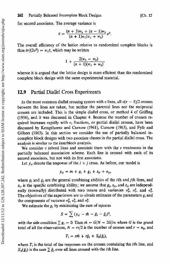
262 Partially Balanced Incomplete Block Designs [Ch. 12
for second associates. The average variance is
_ (n + 3)wi + (n — 1)w2 2 '(n + 1)w1(w1 + w2) a
The overall efficiency of the lattice relative to randomized complete blocks isthus vr/(2o2) = wlv, which may be written
1+ 2(w1 — w2)(n + 1)(w1 + w2)
whence it is argued that the lattice design is more efficient than the randomizedcomplete block design with the same experimental material.
12.9 Partial Diallel Cross Experiments
In the most common diallel crossing system with v lines, all v(v — 1)/2 crossesbetween the lines are taken, but neither the parental lines nor the reciprocalcrosses are included. This is the simple diallel cross, or method 4 of Griffing(1956), and it was discussed in Chapter 4. Because the number of crosses re-quired increases rapidly with v, fractions, or partial diallel crosses, have beendiscussed by Kempthorne and Curnow (1961), Curnow (1963), and Fyfe andGilbert (1963). In this section we consider the use of partially balanced in-complete block designs with two associate classes in the partial diallel cross. Theanalysis is similar to the interblock analysis.
We consider v inbred lines and associate them with the v treatments in thepartially balanced association scheme. Each line is crossed with each of itssecond associates, but not with its first associates.
Let y15 denote the response of the i x j cross. As before, our model is
y,f =m+g,+g5 + siƒ +e15,
where g{ and gi are the general combining abilities of the ith and jth lines, andsi, is the specific combining ability; we assume that g,, s15, and e11 are independ-ently (normally) distributed with zero means and variances a9, as, and ag.The objectives of the experiment are to obtain estimates of the parameters g, andthe components of variance ag, a$, and aé.
We estimate the g, by minimizing the sum of squares
S= (Yir — m — gc — gg)2,
with the side condition 2 g, = 0. Then m = G/N = 2G/rv where G is the grandtotal of all the observations, N = rv/2 is the number of crosses and r = na, and
Ti = rm + rr{ + S2(gt),
where Ti is the total of the responses on the crosses containing the ith line, andS2(fr) is the sum 1 g! over all lines crossed with the ith line.
Dow
nloa
ded
12/1
1/12
to 1
29.1
28.2
07.2
42. R
edis
trib
utio
n su
bjec
t to
SIA
M li
cens
e or
cop
yrig
ht; s
ee h
ttp://
ww
w.s
iam
.org
/jour
nals
/ojs
a.ph
p
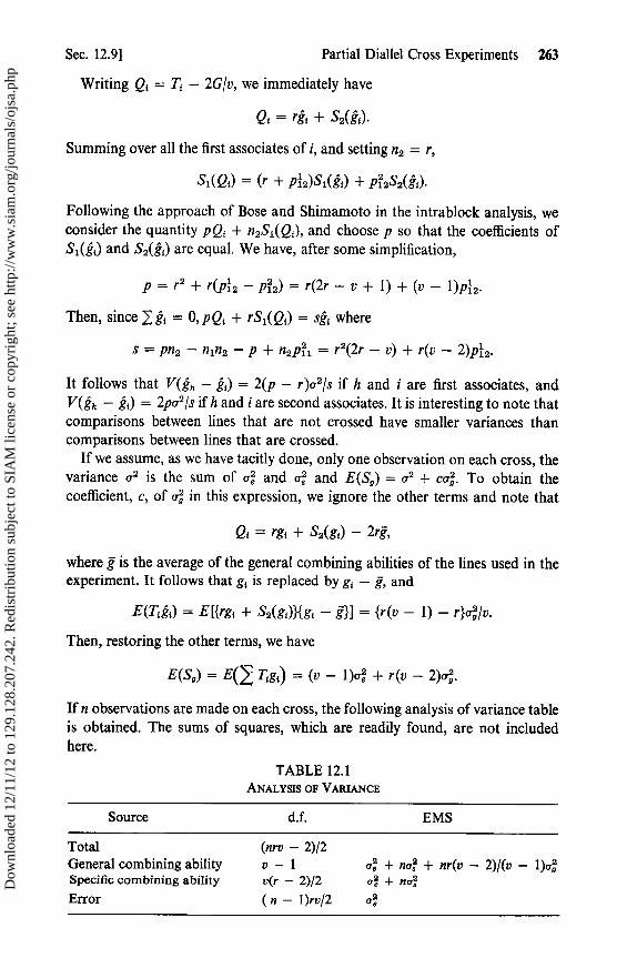
Sec. 12.9] Partial Diallel Cross Experiments 263
Writing Q { = T1 — 2G/v, we immediately have
Qi = rgi + S2(g1)•
Summing over all the first associates of i, and setting nz = r,
S1(Q1) = (r + Pi2)S1(8i) + Pi2S2(g1)•
Following the approach of Bose and Shimamoto in the intrablock analysis, weconsider the quantity pQ i + n2S1 (Q2), and choose p so that the coefficients ofS1(g1) and S2(g1) are equal. We have, after some simplification,
p = r2 + r(P12 — Pi2) = r(2r — v + 1) + (v — 1)P'2•
Then, since g, = 0, pQ ; + rSl(Q,) = sgt where
s = pn2 — n jn2 — p + n2p1 = r2(2r — v) + r(v — 2)Pi2.
It follows that V(gh — gt) = 2(p — r)a2/s if h and i are first associates, andV(gh — g{) = 2pa2/s if h and i are second associates. It is interesting to note thatcomparisons between lines that are not crossed have smaller variances thancomparisons between lines that are crossed.
If we assume, as we have tacitly done, only one observation on each cross, thevariance o2 is the sum of aé and os and E(S9) = a2 + ca9. To obtain thecoefficient, c, of o9 in this expression, we ignore the other terms and note that
Q^ = rgi + S2(gi) — 2rg,
where g is the average of the general combining abilities of the lines used in theexperiment. It follows that g i is replaced by g i — g, and
E(T11) = E[{rgt + S2(gi)}{gi — g}] _ {r(v — 1) — r}ag/v.
Then, restoring the other terras, we have
E(S9) = E( Tigi) = (v — 1)oé + r(v — 2)a9.
If n observations are made on each cross, the following analysis of variance tableis obtained. The rums of squares, which are readily found, are not includedhere.
TABLE 12.1ANALYSIS OF VARIANCE
Source d.f. EMS
Total (nrv — 2)12General combining ability v — 1 oé + no8 + nr(v — 2)/(v — 1)agSpecific combining ability v(r — 2)/2 a + no;
Error (n — 1)rv/2 aé
Dow
nloa
ded
12/1
1/12
to 1
29.1
28.2
07.2
42. R
edis
trib
utio
n su
bjec
t to
SIA
M li
cens
e or
cop
yrig
ht; s
ee h
ttp://
ww
w.s
iam
.org
/jour
nals
/ojs
a.ph
p
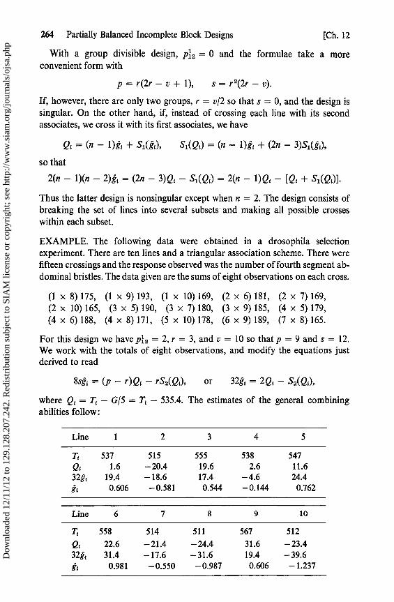
264 Partially Balanced Incomplete Block Designs [Ch. 12
With a group divisible design, p1 2 = 0 and the formulae take a moreconvenient form with
p=r(2r—v+ l), s=r 2(2r—v).
If, however, there are only two groups, r = v/2 so that s = 0, and the design issingular. On the other hand, if, instead of crossing each line with its secondassociates, we cross it with its first associates, we have
Q, = (n — 1 )S, + S1(Si), S1(Q1) = (n — l)gi + (2n — 3)S1(Si),
so that
2(n — 1)(n — 2)Si = (2n — 3)Q j — S1(Q) = 2(n — 1)Q { — [Q + S1(QM)].
Thus the latter design is nonsingular except when n = 2. The design consists ofbreaking the set of lines into several subsets and making all possible crosseswithin each subset.
EXAMPLE. The following data were obtained in a drosophila selectionexperiment. There are ten lines and a triangular association scheme. There werefifteen crossings and the response observed was the number of fourth segment ab-dominal bristles. The data given are the sums of eight observations on each cross.
(1 x 8) 175, (1 x 9) 193, (1 x 10) 169, (2 x 6) 181, (2 x 7) 169,(2 x 10) 165, (3 x 5) 190, (3 x 7) 180, (3 x 9) 185, (4 x 5) 179,(4 x 6) 188, (4 x 8) 171, (5 x 10) 178, (6 x 9) 189, (7 x 8) 165.
For this design we have p1 2 = 2, r = 3, and v = 10 so that p = 9 and s = 12.We work with the totals of eight observations, and modify the equations justderived to read
8sg1 = (p — r)Q1 — rS2(Qi), or 3281 = 2 Qi — S2(Q1),
where Q i = Ti — GIS = Ti — 535.4. The estimates of the general combiningabilities follow:
Line 1 2 3 4 5
Ti 537 515 555 538 547Q, 1.6 —20.4 19.6 2.6 11.632é, 19.4 —18.6 17.4 —4.6 24.4k, 0.606 —0.581 0.544 —0.144 0.762
Line 6 7 8 9 10
Tt 558 514 511 567 512Q, 22.6 —21.4 — 24.4 31.6 —23.432k, 31.4 —17.6 —31.6 19.4 —39.6g, 0.981 —0.550 —0.987 0.606 —1.237
Dow
nloa
ded
12/1
1/12
to 1
29.1
28.2
07.2
42. R
edis
trib
utio
n su
bjec
t to
SIA
M li
cens
e or
cop
yrig
ht; s
ee h
ttp://
ww
w.s
iam
.org
/jour
nals
/ojs
a.ph
p

Sec. 12.10] Choosing an Incomplete Block Design 265
In the analysis of variance the correction for the mean was GIJ120 = 59719.408.The uncorrected sum of squares for crosses was 59870.375, and the uncorrectedsum of squares for individuals y2 (not shown in the data summary) was 60,171.The point estimates of the components of variance were
Qé = 2.863, &s = —0.036, &9 = 0.597.
The analysis of variance table follows:
TABLE 12.2ANALYSIS OF VARIANCE
Source d.f. SS ms EMS
Total 119 451.592(Between crosses) 14 150.967General combining ability 9 138.112 15.346 aé + 8a$ + 21.3309Specific combining ability 5 12.855 2.571 ae + BosIndividuals within crosses 105 300.625 2.863 oé
12.10 Choosing an Incomplete Block Design
The reader has seen in the last two chapters various association schemes forincomplete block designs. In the next three chapters he will see numerousdesigns and recipes for many more. An extensive listing of PBIB(2) designs isgiven in the tables by Bose, Clatworthy and Shrikhande (1954). A listing ofbalanced designs is found in the Fisher and Yates tables (1953). He might wellask how in a given experimental situation he should choose a design from thislong list. It is an easier question to ask than to answer because there is no finalanswer.
Let us suppose that we have fixed upon the number of varieties v and decidedthat a proper, equireplicate design should be used, and that the intrablockanalysis will be used. Kempthorne's conjecture tells us that for any given set ofparameters v, k, N the most efficient incomplete block design is the balanceddesign, if there is one. For that design we have an efficiency factor
_Av v(k-1) v _1E° rk k(v — 1) v — 1 ( 1 k) -
The efficiency depends only upon v and k. For a given v it is an increasingfunction of k.
We should, therefore, try to take k to be as large as we reasonably can. Thereare practical situations in which, although the block size could if necessary beincreased so that k = v, the tost of doing so would be to introduce so muchheterogeneity into the plots that the variance, a2, would be greatly increased.
The efficiency factor E is calculated by comparing the average of V(Th - T{)
Dow
nloa
ded
12/1
1/12
to 1
29.1
28.2
07.2
42. R
edis
trib
utio
n su
bjec
t to
SIA
M li
cens
e or
cop
yrig
ht; s
ee h
ttp://
ww
w.s
iam
.org
/jour
nals
/ojs
a.ph
p
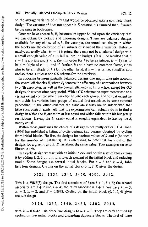
266 Partially Balanced Incomplete Block Designs [Ch. 12
to the average variance of 2a2Ir that would be obtained with a complete blockdesign. The variance a2 does not appear in E because it is assumed that a2 wouldbe the same in both cases.
Once we have chosen k, Eo becomes an upper bound upon the efficiency thatwe can obtain by picking and choosing designs. There are balanced designsavailable for any choice of v, k, for example, the unreduced design in whichthe blocks are the collection of all subsets of k out of the v varieties. Unfortu-nately, especially when (v — 1) is prime, there may not be a balanced design witha small enough value of r to fall within the budget. (It will be recalled that ifv — 1 is a prime and k < v, then, in order for to be an integer, (r — 1) has tobe a multiple of v — 1, and if, further, k and v have no common factor, r hasalso to be a multiple of k.) On the other hand, if v — 1 is prime, v itself is not,and so there is at least one GD scheme for the v varieties.
In choosing between partially balanced designs one might take into accountthe several efficiencies E{ where E{ denotes the efficiency of a comparison betweentwo ith associates, as well as the overall efficiency E. In practice, except for GDdesigns, this is not often very useful. With a GD scheme the experimenter can to acertain extent control which varieties go into each group, and to that extent hecan divide his varieties into groups of mutual first associates by some rationalprocedure. In the other schemes the associate classes are so interlocked thatlittle such control exists. All that the experimenter can actually do is to find adesign in which the E, are more or less equal and which falls within his budgetaryrestrictions. Having the E{ nearly equal is roughly equivalent to having the Atnearly equal.
Within those guidelines the choice of a design is not really critical. J. A. John(1966) has published a listing of cyclic designs, i.e., designs obtained by cyclingfrom initial blocks. He lists the designs for various values of k and v (he uses tfor the number of treatments). It is interesting to note that for most of thedesigns for a given v and k, E has about the same value. Two examples serve toillustrate this.
In a cyclic design we start with an initial block and obtain a set of blocks fromit by adding 1, 2, 3, ..., in turn to each element of the initial block and reducingmod v. Some designs use several initial blocks. For v = 6 and k = 4, Johnlists four designs. Cycling on the initial block (0, 1, 2, 3) gives the design
0123, 1234, 2345, 3450, 4501, 5012.
This is a PBIB(3) design. The first associates of i are i + 1, i + 5; the secondassociates are i + 2 and i + 4; the third associate is i + 3. We have ,1 1 = 3,A, = 2, A = 2, and E = 0.8948. Cycling on the initial block (0, 1, 2, 4) givesthe GD design
0124, 1235, 2340, 3451, 4502, 5013,
with E = 0.8942. The other two designs have r = 6. They are each formed bycycling on two initial blocks and discarding duplicate blocks. The first of these
Dow
nloa
ded
12/1
1/12
to 1
29.1
28.2
07.2
42. R
edis
trib
utio
n su
bjec
t to
SIA
M li
cens
e or
cop
yrig
ht; s
ee h
ttp://
ww
w.s
iam
.org
/jour
nals
/ojs
a.ph
p

Exercises 267
designs is formed from (0, 1, 2, 3) and (0, 1, 3, 4). It has three associate classesand E = 0.8977. The last design is formed from (0, 1, 2, 3) and (0, 1, 3, 4) andhas E = 0.8978. The upper bound is Eo = 0.9000.
John lists nineteen designs for v = 12 and k = 4. They are all partiallybalanced, although two of them have no fewer than six associate classes. Theirefficiencies range from 0.8007 to 0.8166. The value of E, is 0.8182. Two of thedesigns are GD designs. The first has r = 4, E = 0.8138, and initial block(0, 1, 3, 7). The second has r = 10, E = 0.8166, and three initial blocks(0, 1, 2, 5), (0, 1, 3, 8), and (0, 2, 6, 8). There is no advantage in using the morecomplicated association schemes.
In summary, three guidelines are suggested. Take k as large as you reasonablycan. Try to find a design with as much balance as possible. The third guidelineis to choose, subject to the other considerations, the simplest design possible.This is sound advice in the design of any experiment. Keep it as simple as youcan.
Exercises
1. Prove that a sufficient condition for a PBIB(2) scheme to be group divisible is thateither pis = 0 or piz = 0.
2. Show that A,. = k206.
3. Derive the constant d l in the Bose—Shimamoto form of the combined intrablockand interblock estimates.
4. Prove that for a GD design the methods of Yates and Rao give the same com-bined estimates for comparing first associates.
5. Show that for the simple lattice the methods of Yates and Rao do not give thesame combined estimates.
6. Derive the formula given for V(Th - T*) in the simple lattice.
Dow
nloa
ded
12/1
1/12
to 1
29.1
28.2
07.2
42. R
edis
trib
utio
n su
bjec
t to
SIA
M li
cens
e or
cop
yrig
ht; s
ee h
ttp://
ww
w.s
iam
.org
/jour
nals
/ojs
a.ph
p

CHAPTER 13
The Existence andConstruction of
BalancedIncomplete
Block Designs
Balanced incomplete block designs were introduced and discussed in Chapter11 and partially balanced incomplete blocks in Chapter 12. This chapter and thenext two are devoted to the construction of designs. The problems that we shallconsider are essentially problems in combinatorial mathematics. Many of thecontributions to the construction of balanced incomplete block designs havebeen made by algebraists who had no other interest in statistics. Some of theirresults antedate the discovery of balanced incomplete block designs by manyyears.
This chapter and the next two are quite different from the preceding chapters.They presuppose more knowledge of abstract algebra. The reader who is notinterested in this topic can safely omit this and the next two chapters; if he wantsa balanced incomplete design for a given practical situation he can get it easilyenough, if it exists, from the Fisher and Yates tables. On the other hand, theresearch student in mathematical statistics will find in these chapters that thereremain numerous questions to be answered. The algebraist who knows nostatistics might find them interesting reading, and he will need only to refer backto Chapters 11 and 12; he does not need to know anything about the analysis ofvariance, or, indeed, why the statistician cares about these designs at all. In theinterest of completeness, we shall begin by repeating some basic material fromChapter 11.
Balanced incomplete designs were introduced by Yates (1936) for use inagricultural experiments, and the agricultural terminology has remained in thejargon. A balanced incomplete block design, or BIBD, is a collection of b blocks,
Dow
nloa
ded
12/1
1/12
to 1
29.1
28.2
07.2
42. R
edis
trib
utio
n su
bjec
t to
SIA
M li
cens
e or
cop
yrig
ht; s
ee h
ttp://
ww
w.s
iam
.org
/jour
nals
/ojs
a.ph
p

Construction of Balanced Incomplete Block Designs 269
each consisting of k plots; v treatments, or varieties (v > k), are assigned to theplots (one treatment to each plot) in such a way that
(i) Each treatment appears exactly r times;(ii) No treatment appears more than once in any block (a design with this
property is called a binary design);(iii) Each pair of treatments appears together in exactly A blocks.
The five parameters b, v, r, k, ) are not independent. They satisfy the conditions:
(a) bk = rv = N, which is the total number of plots;(b) A = r(k — 1)/(v — 1), which is an integer;(c) b >_ v.
The inequality was proved by Fisher (1940), and is called Fisher's inequality.It was derived in Chapter 11, and the derivation is repeated here.
The 1938 edition of the Fisher and Yates tables contained a list of all sets ofparameters satisfying conditions (a) and (b) with r < 10 for which designs wereknown to exist, in which case the design was given, and those for which it wasnot yet known whether or not designs existed. Bose (1939) solved all the un-known cases in the listing except for twelve. Later workers have reduced thenumber of unsolved cases in his list to two. The two open cases are b = 69,v = 46, r = 9, k = 6, A = 1, and b = 85, v = 51, r = 10, k = 6, A = l; it isstill not known whether designs exist in these cases. Rao (1961) published a listof all sets of parameters with 11 < r < 15, satisfying conditions (a) and (b),together with known solutions, and Sprott (1962) did the same for 16 < r < 20.Bose's 1939 paper is the major work in the field, and we shall draw heavilyupon it in this chapter.
Associated with any incomplete block design is its incidence matrix N = (n 1).N is a matrix of v rows and b columns, and n,f is the number of times that the ithvariety appears in thejth block. For a BIBD, the elements of N are either zero orone, and NN' = (r — ,1)I„ + AJ„ where J„ is the square matrix of order v, eachelement of which is unity.
The determinant NN' = (r — A)" - '(r + (v — 1)A) = (r — )'_'rk, which ispositive since A < r.
Thus the rank of NN' is r(NN') = r(N) = v; but r(N) < min (b, v), and sob >— v.
If b = v and r = k the design is said to be symmetric. For such a design N is asquare matrix and INN'I = 1N1 2. This implies that (r — ))v -1 is a square.Hence, if v is even, a necessary condition for the existence of a symmetric designis that (r — )) is a perfect square. This nonexistence theorem was derivedindependently by Schutzenberger (1949), Shrikhande (1950), and Chowla andRyser (1950). It shows that conditions (a), (b), and (c) are not sufficient for theexistence of a design. Consider, for example, the case b = v = 22 and r = k =7; we have A = 2, and so r — ^1 = 5, and no such design exists.
Dow
nloa
ded
12/1
1/12
to 1
29.1
28.2
07.2
42. R
edis
trib
utio
n su
bjec
t to
SIA
M li
cens
e or
cop
yrig
ht; s
ee h
ttp://
ww
w.s
iam
.org
/jour
nals
/ojs
a.ph
p

270 Construction of Balanced Incomplete Block Designs [Ch. 13
The simplest series of balanced incomplete block designs are the unreduceddesigns; these are the designs that consist of all possible combinations of kout of the v varieties. For these designs
b=() r=() A — (k — 2).
It is not necessary to investigate cases for which 2k > v. If a new design of bblocks and v varieties is formed by assigning to each block those varieties thatdo not appear in the corresponding block of the BIBD, the new design is alsoa BIBD; it is called the complementary design.
13.1 The Orthogonal Series
These two series of designs, introduced by Yates (1936), depend upon theexistence of a series of s + 1 orthogonal Latin squares of side s; such sets ofsquares are known to exist whenever s = pm where p is a prime.
For the first series, b = s(s + 1), v = s 2, r = s + 1, k = s, and \ = 1. Thes 2 + s blocks fall into s + 1 sets of s blocks each. In each set every treatmentappears exactly once, and the set forms a complete replicate of all the varieties.A design that can be divided into complete replicates is called resolvable. Eachset can be denoted by a square array of s 2 plots with the rows of the arraycorresponding to blocks. The varieties are denoted by the integers 1, 2, ..., s 2 .
In the first set the jth row, and hence, the jth block, consists of the varieties(j — 1)s + 1,(j— 1)s+ 2,...,(j— 1)s + s = js. The rows in the second setare the columns in the first set; the jth row consists of j, j + s, j + 2s,...,j + (s — 1)s. The remaining sets make use of the orthogonal Latin squares. Con-sider one of the squares composed of letters A, B, C, .... The corresponding setof blocks is obtained by superimposing the Latin square on the square array of thefirst set. Then the varieties in the first row of the new set are those that coincidewith the letter A; the second row contains varieties coinciding with B, and so on.
We illustrate the procedure with an example for s = 4. A set of three orthog-onal squares has already been obtained in the chapter on Latin squares, inwhich Bose's method of obtaining orthogonal sets was presented. The design,which was given in Chapter 11, is
1 2 3 4 15 913 161116 171214 1810155 6 7 8 261014 251215 281113 27 9169101112 371115 38 914 351016 361213
13 14 15 16 481216 47 10 13 46 915 451114.
To show that the design is a BIBD, we note that any pair of varieties cannotappear together in more than one block. If they appear in the same block of thefirst set, they cannot appear in the same row of the second set, and vice versa;in neither case can they appear in the same block in one of the subsequent sets,
Dow
nloa
ded
12/1
1/12
to 1
29.1
28.2
07.2
42. R
edis
trib
utio
n su
bjec
t to
SIA
M li
cens
e or
cop
yrig
ht; s
ee h
ttp://
ww
w.s
iam
.org
/jour
nals
/ojs
a.ph
p

Sec. 13.2] Series of Designs Based on Finite Geometries 271
for that would imply that the same letter appeared twice in the same row (orcolumn) of a Latin square. Similarly, if a pair of varieties appears together in ablock of the (i + 2)th set and also in a block of the (h + 2)th set, that contra-dicts the fact that the ith and hth squares are orthogonal. However, each varietyappears r = s + 1 times, once in each set, and thus its plots appear in the sameblocks as r(k — 1) = s 2 — 1 plots occupied by other varieties; if no variety isto appear more than once, these 2 — 1 plots must be taken up by each of theother varieties appearing once each, and the design is a BIBD with A = 1.
Conversely, the existence of a BIBD with parameters b = s(s + 1), v = s 2 ,
r = s + 1, k = s, and A = 1 implies the existence of a set of s — 1 orthogonalsquares of side s. This establishes the nonexistence of a design with b = 42,v = 36, r = 7, k = 6, and A = 1 since there is not a complete set of Latinsquares of side six.
To each member of the first series, OSI, there corresponds a member of thesecond series, 0S2. These are designs for v = S 2 + s + 1 varieties. To eachblock of the ith set of the OS1 design an extra plot is added containing the(s 2 + i)th variety. One extra block is added, consisting of one plot with each ofthe new varieties. The resulting design is a BIBD with b = v = s 2 + s + 1,r = k = s + 1, and A = 1. There is no such design for forty-three varieties.The designs of the first series are also called balanced lattices; any two of thereplicate sets constitute a simple lattice.
13.2 Series of Designs Based on Finite Geometries
Let s = p" be a prime or a power of a prime. A point in the finite projectivegeometry PG(N, s = pn) is represented by a (N + 1)-tuple, each coordinate ofwhich is an element of the Galois field GF(s), and not all of which are zero.We write x = (x0 , x 1 ,. . ., xN), xt e GF(s). Two points, x and y, are identical ifthere exists an element 6 of the field such that xt = Oy, for all i.
Altogether there are sN+l — 1 such (N + 1)-tuples. They may be divided intogroups of (s — 1) members with each member of the same group representing thesame point. Thus the geometry PG (N, s) has (sN+ 1 — 1)/(s — 1) distinct points.
Let x and y be two of these points. The line joining x and y is the set of allpoints A 1x + a2y where Al, A2 E GF(s). There are (s + 1) distinct points on thisline (or one-dimensional subspàce), namely y, which corresponds to A l = 0,X12 = 1, and the s points obtained by putting A l = 1 and letting X12 take all svalues in the field. The point x is joined by lines to Bach of the other points; eachof these lines contains s points in addition to x, and none of the points lies onmore than one of the lines. Hence, [(s'+ 1 — 1)/(s — 1) — 1 ]/s = (5N — 1)/(s — 1)lines pass through x. Altogether there are
sN+1 — 1 5N_1 1 (SN+1 — l)(SN — 1)
S -1 S -1 S +1 (s2- 1)/(\s-1)
lines, and each pair of points appears on one and only one line.
Dow
nloa
ded
12/1
1/12
to 1
29.1
28.2
07.2
42. R
edis
trib
utio
n su
bjec
t to
SIA
M li
cens
e or
cop
yrig
ht; s
ee h
ttp://
ww
w.s
iam
.org
/jour
nals
/ojs
a.ph
p

272 Construction of Balanced Incomplete Block Designs [Ch. 13
If we now let the points represent varieties and the lines represent blocks, thesystem of points and lines gives a BIBD with
SN+1 — 1 (SN+1 — 1)(SN — 1)
v s-1 b=l (s2-1) (s -1) 'k=s+1, a=1.
If N = 2, we have the orthogonal series with b = v = s 2 + s + 1, r = k =s+1.
The simplest example occurs when s = N = 2. Then s takes the valnes 0, 1,and the arithmetic is carried out mod 2. The seven points are A (100), B (010),C (001), D (011), E (101), F (110), G (111). The seven lines are x o = 0, BCD;xl = 0, ACE; x2 = 0, ABF; x o + xl - 0, CFG; xo + x2 - 0, BEG; xl + x2
0, ADG; xo + xl + x2 = 0, DEF. This design may also be obtained from thegeometrical figure of the complete quadrangle, using as blocks the six sides andthe live consisting of the three points in which the pairs of opposite sides meet.
We now extend these ideas from one-dimensional subspaces to m-dimensionalsubspaces. Let pi, i = 1, 2, ..., m + 1 be a set of (m + 1) points whose co-ordinate vectors are linearly independent; denote the vectors by p i . The set ofpoints whose coordinate vectors are linear combinations ,l ip{ forms an m-dimensional subspace of PG (N, s). If t = µi for all i, the two linear combinations1 Alyi and 1 µ,p i denote the same point. Thus the sets of coefficients {^1,} them-selves represent the points of PG(m, s). Hence, the number of points in anm-dimensional subspace is the same as the number of points in PG(m, s),namely (sm+l — 1)/(s — 1).
To obtain an ordered set of (m — 1) linearly independent points fromPG(N, s), we may choose the first point in (sN+' — 1)/(s — 1) ways, and thesecond point in {(sN+1 — 1)/(s — 1)} — 1 ways; for the third point the choice islirnited to those points that do not belong to the one-dimensional subspacegenerated by the first two points; it may be chosen in {(sN+1 — 1)/(s — 1)} —
{(s 2 — 1)/(s — 1)} ways. Similarly, the (i + 1)th point may be chosen in{(S +1 — 1)/(s — 1)} — {(s t — 1)/(s — 1)} = {s' (SN - i+1-1)}/(s — 1) ways. Hencethere exist rj {st(sN-1+1 — 1)/(s — 1)} ordered sets of (m — 1) independentpoints in PG (N, s). By a similar argument there are n {s{(sm-s+1 — 1)/(s — 1)}ordered sets of (m — 1) points in each PG(m, s). Taking the quotient we havefor the number of m-dimensional subspaces in PG(N, s)
(s" — 1)(SN — 1). .. (SN-m+l — 1)
D(N, m, s) =(Sm+1 — 1)(Sm
1). ..
1)l. .. (S — 1)
Each point belongs to
(SN+1 — 1)(SN — 1) ... (SN - m+1 — 1) x (sm+l — 1) = ^(N — 1, m — 1, s)(m+1 —1 1)(Sm — 1) ... (s — 1) (SN+1 — 1)
subspaces and each pair of points belongs to 1(N — 2, m — 2, s) subspaces.
Dow
nloa
ded
12/1
1/12
to 1
29.1
28.2
07.2
42. R
edis
trib
utio
n su
bjec
t to
SIA
M li
cens
e or
cop
yrig
ht; s
ee h
ttp://
ww
w.s
iam
.org
/jour
nals
/ojs
a.ph
p

Sec. 13.2] Series of Designs Based on Finite Geometries 273
We may now identify points with varieties and subspaces with blocks toobtain BIB designs with parameters
/SN+1 _ 1v = I ) _ '(N, 0, s); b= t(N, m, s); r= J?(N — 1,m— 1, s);
, s-1
k = (sm+l _ 1 \
—I = ^(m,0,2); A = O(N— 2, m — 2, s),
s1 /
where I(N, —1, s) = 1. The subspaces, or m-flats, are obtained as the sets ofpoints satisfying sets of (N — m) linear restrictions of the form = 0.
EXAMPLES. PG(3, 2). All arithmetic is mod 2; N = 3, s = 2. There arefifteen points.
1. 0001 2. 0010 3. 0011 4. 0100 5. 0101 6. 0110
7. 0111 8. 1000 9. 1001 10. 1010 11. 1011 12. 1100
13. 1101 14. 1110 15. 1111.
For m = 2, each flat is defined by a single equation and the design bas b = v = 15,r = k = 7, and i\ = 3. The blocks are
xa - 0
x1 -0x2 = 0x3 =_ 0
xo +x1 =0xo +x2 -0x0+xg- 0x1 +x2 =0x1 +x3 -0x2 + x3 0
xo +xl +x2 -0x0 + x1 + x3 0xo + x2 + x3 = 0xl + x2 + x3 - 0
xo +x 1 +x2 +x3 -0
123 4 5 6 7,123 8 9 10 11,145 8 91213,246 8101214,1 2 3 12 13 14 15,1 4 5 10 1114 15,246 9 11 13 15,167 8 91415,257 8101315,347 8111215,1 6 7 10 1112 13,257 911 1214,347 9101314,356 8111314,356 9101215.
If we take the intersections of pairs of two-flats, we obtain the design form = 1 with b = 35 and k = 3. Equating any two linear combinations to zeroalso equates their sum to zero, and so the intersections are actually intersectionsof three two-flats. For example, x2 + x3 = 0, xo - 0, and xo + x2 + x3 - 0give the block 3, 4, 7; xo =_ 0, x l = 0, and xo + x l - 0 give 1, 2, 3; x o + x 3 = 0,xo + xl + x2 = 0, and x l + x2 + x3 = 0 give the block 6, 11, and 13.
Dow
nloa
ded
12/1
1/12
to 1
29.1
28.2
07.2
42. R
edis
trib
utio
n su
bjec
t to
SIA
M li
cens
e or
cop
yrig
ht; s
ee h
ttp://
ww
w.s
iam
.org
/jour
nals
/ojs
a.ph
p
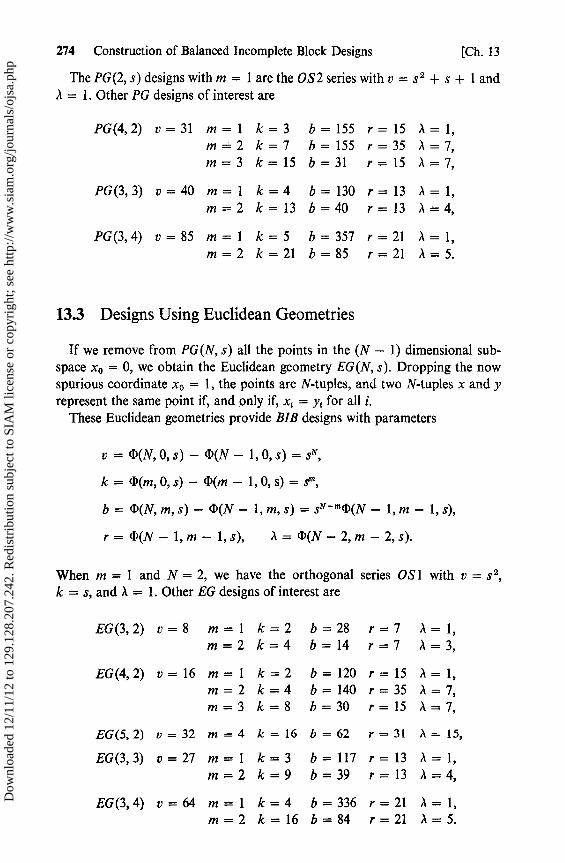
274 Construction of Balanced Incomplete Block Designs [Ch. 13
The PG(2, s) designs with m = 1 are the 0S2 series with v = s 2 + s + 1 andA = 1. Other PG designs of interest are
PG(4,2) v=31 m=1 k=3 b=155 r=15 A=1,m=2 k=7 b=155 r=35 )=7,m=3 k=15 b=31 r=15 )=7,
PG(3,3) v=40 m=1 k=4 b=130 r=13 A=1,m=2 k=13 b=40 r=13 )=4,
PG(3,4) v=85 m=1 k=5 b=357 r=21 A=1,m=2 k=21 b=85 r=21 ^t=5.
13.3 Designs Using Euclidean Geometries
If we remove from PG(N, s) all the points in the (N - 1) dimensional sub-space xo = 0, we obtain the Euclidean geometry EG(N, s). Dropping the nowspurious coordinate xo = 1, the points are N-tuples, and two N-tuples x and yrepresent the same point if, and only if, x, = yi for all !.
These Euclidean geometries provide BIB designs with parameters
v=D(N,0, ․)- b(N- 1,0, ․)=sN,
k = 'J?(m, 0, s) - (D(m - 1, 0, s) = s-,
b = t(N, m, s) - (D(N - 1, m, s) = sN - m<D(N - 1, m - 1, s),
r = (D(N- 1, ni- 1, s), .1 = '(N-2,m-2, ․ ).
When m = 1 and N = 2, we have the orthogonal series OS 1 with v = s 2,k = s, and A = 1. Other EG designs of interest are
EG(3,2) v=8 m=1 k=2 b=28 r=7 .1=1,m=2 k=4 b=14 r=7 A=3,
EG(4,2) v=16 m=1 k=2 b=120 r=15 .1=1,m=2 k=4 b=140 r=35 A=7,m=3 k=8 b=30 r=15 ,1=7,
EG(5,2) v=32 m=4 k=16 b=62 r=31 A=15,
EG(3,3) v=27 m=1 k=3 b=117 r=13 A=1,m=2 k=9 b=39 r=13 A=4,
EG(3,4) v=64 m=1 k=4 b=336 r=21 A=1,m=2 k=16 b=84 r=21 A=5.
Dow
nloa
ded
12/1
1/12
to 1
29.1
28.2
07.2
42. R
edis
trib
utio
n su
bjec
t to
SIA
M li
cens
e or
cop
yrig
ht; s
ee h
ttp://
ww
w.s
iam
.org
/jour
nals
/ojs
a.ph
p

Sec. 13.4]
Designs Derived from Difference Sets 275
13.4 Designs Derived from Difference Sets
Let G: (xo = 0, x1 , ..., xv _ 1) be an Abelian group of v elements with additionas the group operation. We can associate each treatment with a different elementof the group. If v is a prime, the set of residue classes mod v is a convenient groupfor our purposes; we associate the treatments with the integers 0, 1, ..., v - 1,and reduce all sums mod v. Let D = (dl , d2 ,. . ., dk) be a proper subset of Gsuch that every element of G, except xo , can be expressed in exactly A ways as adifference d, - d;. Then D is called a perfect differente set, or, more con-veniently, a difference set. If D i = (dl + xi , d2 + x{ , ..., dk + x i), xj E G, thenD. is also a difference set. It will be proved in a more general context that thecollection of all v difference sets Di forms a symmetric BIBD with b = v andr = k. These designs are called cyclic designs; their incidente matrices arecirculants. The set D is called the initial block.
For v = 7 we may take the group of residue classes mod 7. Consider the setD = (0, 1, 3); dl - d2 6, d2 - d1=1, d1 - d3 4, d3 - d1=3, d2 - d35, d3 - d2 - 2, and each difference other than zero appears exactly once. Wemay, therefore, take D as an initial block. Adding 1 to each element of D givesD l = (1, 2, 4); adding 2 gives (2, 3, 5), and so on. This gives a design for seventreatments in seven blocks of three. The blocks are
0, 1, 3; 1, 2, 4; 2, 3, 5; 3,4,6; 4, 5, 0; 5, 6, 1; 6, 0, 2.
The complementary design with k = 4 and A = 2 is generated in a similar wayfrom the initial block (0, 2, 3, 4).
A difference set for v = 15 and k = 7 can be obtained by representing eachtreatment by a pair of integers (x, y), x = 0, 1, 2, 3, 4, y = 0, 1, 2. Addition isdefined by (x1 , y l) + (x2 , Y2) = (x1 + x2 , yl + y2) with x l + x2 reduced mod 5,and yl + Y2 reduced mod 3. The design is
00, 10, 40, 01, 21, 31, 02;10,20,00, 11, 31,41, 12;20, 30, 10,21,41,01,22;30, 40, 20, 31, 01, 11, 32;40,00,30,41,11,21,42;
01,11,41,02,22,32,00;11, 21, 01, 12, 32, 42, 10;21, 31, 11,22,42,02,20;31, 41, 21, 32, 02, 12, 30;41, 01, 31, 42, 12, 22, 40;
02, 12, 42, 00, 20, 30, 01;12, 22, 02, 10, 30, 40, 11;22, 32, 12, 20, 40, 00, 21;32,42,22,30,00,10,31;42, 02, 32, 40, 10, 20, 41.
If v is a power of a prime, we may use the Galois field GF(v) in a mannersimilar to the double modulus system just mentioned. For example, if v = 16and k = 6 the treatments are represented by elements of the form ao + alx +a2x2 + a3x3 where the coefficients a; are either zero or one. Arithmetic is carriedout mod 2. The representations of the treatments can be abbreviated to the4-tuples a1a2a3a4 . The initial block is 0000, 0001, 1000, 1111, 0101, 0011.
We shall see later that the use of difference sets may be extended to includedesigns involving several initial blocks. If there are t initial blocks, the design
Dow
nloa
ded
12/1
1/12
to 1
29.1
28.2
07.2
42. R
edis
trib
utio
n su
bjec
t to
SIA
M li
cens
e or
cop
yrig
ht; s
ee h
ttp://
ww
w.s
iam
.org
/jour
nals
/ojs
a.ph
p
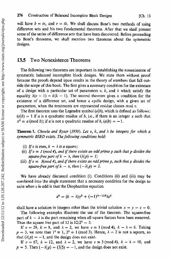
276 Construction of Balanced Incomplete Block Designs [Ch. 13
will have b = tv, and r = tk. We shall discuss Bose's two methods of usingdifferente sets and his two fundamental theorems. After that we shall presentsome of the series of difference sets that have been discovered. Before proceedingto Bose's theorems, we shall mention two theorems about the symmetriedesigns.
13.5 Two Nonexistence Theorems
The following two theorems are important in establishing the nonexistence ofsymmetrie balanced incomplete block designs. We state them without proofbecause the proofs depend upon results in the theory of numbers that fall out-side the scope of this book. The first gives a necessary condition for the existenceof a design with a particular set of parameters v, k, and A which satisfy theequality A(v — 1) = k(k — 1). The second theorem gives a condition for theexistence of a difference set, and hence a cyclic design, with a given set ofparameters, when the treatments are represented residue classes mod v.
The first theorem uses the Legendre symbol (alb), which is defined as follows:(alb) = 1 if a is a quadratic residue of b, i.e., if there is an integer x such thatx2 = a (mod b); if a is not a quadratic residue of b, (alb) = —1.
Theorem 1. Chowla and Ryser (1950). Let v, k, and A be integers for which asymmetric BIBD exists. The following conditions hold:
(i) If v is even, k — A is a square;(ii) If v - 1 (mod 4), and if there exists an odd prime p such that p divides the
square free part of k — , then (Al p) = 1;(iii) If v = 3(mod 4), and if there exists an odd prime p, such that p divides the
square free part of k — A, then (— Ai p) = 1.
We have already discussed condition (i). Conditions (ii) and (iii) may becombined into the single statement that a necessary condition for the design toexist when v is odd is that the Diophantine equation
x2 = (k — A)y2 + (- 1)cv_ 2Az2
shall have a solution in integers other than the trivial solution x = y = z = 0.The following examples illustrate the use of the theorem. The square-free
part of k — A is the part remaining when all square factors have been removed.Thus the square free part of 12 is 12/2 2 = 3.
If v = 29, k = 8, and A = 2, we have v - 1 (mod 4), k — ,1 = 6. Takingp = 3, we note that 1 2 = 1, 22 = 1 (mod 3). Hence, A = 2 is not a square, sothat (Alp) = —1, and the design does not exist.
If v = 67, k = 12, and ,1 = 2, we have v=— 3 (mod 4), k — 1 = 10, andp = 5. Then (—) p)p) = (315) = —1, and the design does not exist.
Dow
nloa
ded
12/1
1/12
to 1
29.1
28.2
07.2
42. R
edis
trib
utio
n su
bjec
t to
SIA
M li
cens
e or
cop
yrig
ht; s
ee h
ttp://
ww
w.s
iam
.org
/jour
nals
/ojs
a.ph
p

Sec. 13.6] The Fundamental Theorems of Bose 277
Theorem 2. Hall and Ryser (1951). Let v be odd and let e be any positive divisorof v. A necessary condition for the existence of a symmetric design with parametersv, k, and A, which is cyclic, is that the Diophantine equation
x2 = (k — A)y2 + (- 1)(e- 1)12eZ2
must possess a solution in integers that are not all zero.
Smith and Hartley (1948) showed that if, for any design with v = b and r = k(whether balanced or not), we write the design as a rectangular array of v rowsand k columns with blocks as rows, it is possible to arrange the treatmentswithin the rows in such a way that each treatment appears exactly once in eachcolumn. Such an arrangement is called a Youden square; in the analysis, a sumof squares can be taken for differences between columns if desired.
It does not follow, however, that every symmetric design is a cyclic design, oris isomorphic to one in t1 e sense that it could be made cyclic by a suitablerelabeling of the treatments. Bhattacharya (1944b) has obtained a symmetricBIBD for v = 25, k = 9, and A = 3.
Bhattacharya's design is the following:
ABEFKLQTW ABIJOPQUY ABMNGHQVXCDEFOPQVX ADEHJKSVY ADILNOSTXBCMPJKSTX BCEHNOSUW ACEGJLRUXBDIKFHRUX DBMOJLRVW BDEGNPRTYEIMHLPWXY GKOHLPQRS FJNHLPTUV
CDIJGHQTW CDMNKLQUYADMPFGSUW BCILFGSVYACIKNPRVW ACMOFHRTYEIMFJNQRS EIMGKOTUVFJNGKOWXY QRSTUVWXY.
However, the equation
x2 = 6y2 + 5z2
has no solution in integers, other than x = y = z = 0, and so there can be nocyclic design with these parameters.
13.6 The Fundamental Theorems of Bose
We now extend this concept of generating a design from a difference set toBose's methods of symmetrically repeated differences. We consider, as before,an Abelian group G with m elements (xo = 0, x l , ... , x,n - 1); the group operationis addition.
Dow
nloa
ded
12/1
1/12
to 1
29.1
28.2
07.2
42. R
edis
trib
utio
n su
bjec
t to
SIA
M li
cens
e or
cop
yrig
ht; s
ee h
ttp://
ww
w.s
iam
.org
/jour
nals
/ojs
a.ph
p

278 Construction of Balanced Incomplete Block Designs [Ch. 13
Let v = mn treatments be divided into m subsets of n treatments each. Weassociate one subset with each element of the group G, and denote by viƒ the jthof the treatments in the subset, which has been assigned to the element x i ;treatments with the same second subscript, j, are said to belong to the same class.The notation used by Bose is to denote each treatment by the numeral of itssubset, i, with the numeral, j, of its class as a subscript; thus our v 12 would bedenoted by 1 2 .
Suppose that a block contains k treatments, of which m; belong to the jthclass. There are two kinds of differences to be considered: pure differences[j, j] and mixed differences [j, j'], j # j'. The pure differences [j, j] are themi(mj - 1) differences of the type (x i - x;.) where xt and x,. correspond totreatments vtf and v; • f in the block; the mixed differences [j, j'] are the mimi .differences of the type (x { - x{ .) where xi, x; - correspond to treatments vif andvi ,j, in the block (we may have i = i'). If n = 1 there are no mixed differences,and we have the situation considered in the previous sections.
For example, if G consists of the residue classes, mod 5, and n = 2, there areten treatments; consider the block 0 1 , 1 1 , 3 1 , 32 , and 42 . The differences [1, 1] are0-1=4, 0-3=2, 1-3=3, 1-0=1, 3-0=3,3-1=2. Thedifferences [2, 2] are 3 - 4 = 4 and 4 - 3 = 1. The differences [1, 2] are0-3=2, 1-3=3, 3-3=0, 0-4=1, 1-4=2, 3-4=4. Thedifferences[2, 1]are3 -0 = 3,3-1 = 2,3-3 = 0,4-0 = 4,4-1 = 3,4 - 3 = 1.
Consider now a set of t blocks satisfying the following conditions, where m1,denotes the value of mf in the sth block:
(i) For each j the set of , m ;s(m;s - 1) pure differences [j, j] contains eachnonzero element of G exactly 2 times;
(ii) For each pair j, j'(j j') the set of 1s m;sm; .s mixed differences [j, j']contains each element of G, including zero, exactly A times.
We say that in these t blocks the differences are symmetrically repeated.For example, if G is the set of residue classes mod 5, and n = 2, the following
set of t = 6 blocks has the property with A = 2: 0 2 , 1 2 , 22 ; 1 1 , 4, 02 ; 2, 3 1 , 02 ;11, 4, 22; 2^, 3 , 22; 01, 02, 22.
Theorem 1. The first fundamental theorem of differences:Let G be an Abelian group of m elements, and let v = mn treatments be dividedinto m subsets of n treatments each, denoted by v i;, as described previously.Suppose that we canfind a set of t blocks B 1 , B2,. . . , Bi which satisfy the followingconditions:
(i) Each block has k plots and contains k different treatments;(ii) Among the kt varieties occurring in the set of t blocks, exactly r belong to
each class. (Some treatments may appear 'in more than one block, and eachappearance is counted; thus kt = nr);
(iii) The differences are symmetrically repeated, A times each, in the t blocks.
Dow
nloa
ded
12/1
1/12
to 1
29.1
28.2
07.2
42. R
edis
trib
utio
n su
bjec
t to
SIA
M li
cens
e or
cop
yrig
ht; s
ee h
ttp://
ww
w.s
iam
.org
/jour
nals
/ojs
a.ph
p

Sec. 13.6] The Fundamental Theorems of Bose 279
Suppose further that these t blocks are used as initial blocks in the followingmanner. From each initial block B, a set of m blocks is generated. If v h; is atreatment in B3, and Xg = Xh + x t , thèn v9j appears in B P ; the block B30 is theinitial block B.
The theorem states that the resulting set of mt blocks forms a balanced incom-plete block design with v = mn, b = mt, r, k, A.
PROOF. Let Vhj be a treatment in B3. The images of Vhj in the set of blocks B8
consist of all treatments v l, belonging to the jth class. Thus each treatment vif
appears in the design exactly once for each appearance of j in the initial blocks.Hence, by virtue of condition (ii), each treatment v t5 , i = 0, 1, ..., m - 1,j = 1, 2, ..., n, appears exactly r times in the set of mt blocks.
Consider two treatments: v ij and vt .; ., j j'. They appear together in a block'B39 if, and only if, we can find two treatments v, ti5 and vh . ;- in B, and an elementXg in G such that Xh + x9 = xj and Xh ' + Xg = xi.. Subtracting, we have theequivalent condition Xh - xh, = x, - xj . This implies that the pair v, 1, vi .; . occursin exactly one of the blocks generated by B, whenever i - i' is one of thedifferences [j, j'] in that block. However, the difference i - i' occurs exactly Atimes among the set of differences [j, j'] in all t blocks, and so the pair of treat-ments vtƒ , vn ', occurs together in exactly ) blocks of the design. A similarargument involving the nonzero differences [j, j] shows that the pair v;5, vl -f alsooccurs together exactly A times. Thus the design is a balanced incomplete blockdesign with the required parameters, and the theorem is proved. E
It should be noted that the requirement that each of the initial blocks shouldcontain exactly k plots has not been used. Even if the blocks are of differentsizes, the resulting design, though not a BIBD, is stilt equireplicate, and eachpair of treatments appears in the same block exactly ,1 times.
EXAMPLE 1. The six blocks with k = 3, v = 10 just given may be used asinitial blocks for a design with parameters v = 10, b = 30, r = 9, k = 3, A = 2.
The complete design is
02,12,22; 11,41,02; 21,3 1 ,02 ; 1 1, 41, 22; 21,3 1 ,22 ; 01,02 ,22 ;
1 2, 22, 32; 21, 01, 1 2; 31, 41, 1 2; 21, 01, 32; 31, 41, 32; 11, 1 2, 32;
22, 32, 42; 3 1, 1 1, 22; 41, 01, 22; 31, 1 1, 42; 41, 01, 42; 21, 22, 42;
32, 42, 02; 41, 21, 32; 01, 1 1, 32; 41, 21, 02; 01, 1 1, 02; 31, 32, 02;
42, 02, 1 2; 01, 31, 42; 11, 21, 42; 01, 31, 1 2; li, 21, 1 2; 41, 42, 1 2.
EXAMPLE 2. v = 9, b = 18, r = 8, k = 4, and A = 3. Gis the set of residueclasses mod 9, m = 9, n = 1. The initial blocks are 0, 1, 2, 4; 0, 3, 4, 7.
EXAMPLE 3. v = 25, b = 50, r = 8, k = 4, i\ 1. G is the set of residueclasses of the double modulus system mod (5, 5), or, equivalently, G can be theGalois field GF(5 2). The initial blocks are 00, 01, 41, 13; 00, 32, 21, 02.
Dow
nloa
ded
12/1
1/12
to 1
29.1
28.2
07.2
42. R
edis
trib
utio
n su
bjec
t to
SIA
M li
cens
e or
cop
yrig
ht; s
ee h
ttp://
ww
w.s
iam
.org
/jour
nals
/ojs
a.ph
p

280 Construction of Balanced Incomplete Block Designs [Ch. 13
We begin the discussion of Bose's second method by considering an example.We can obtain two symmetric designs for v = 7: a design with k = 3, ,1 = 1,and the complementary design with k = 4, A = 2. If we take the smaller designand add to each block a fourth plot with a new (eighth) treatment, then allfourteen blocks comprise a balanced incomplete block design with v = 8,b = 14,r = 7,k = 4,andA = 3.
This approach can be generalized. We need to find two BIBD, one withparameters v, b 1 , r1 , k, A l , and the other with parameters v, b2 , r2, k — 1, ,12 .
To each block of the second BIBD we add an extra plot with a new treatment oo.If the composite design is a BIBD, its parameters must be v + 1, b = bl + b2 ,
r = rl + r2 , k, = + a2. In the latter design the treatment oo appears in b2
blocks, and each of the old treatments appears in rz of these. We must, therefore,have r2 = A and r = b2, whence blk = b2(v — k + 1).
Theorem 2. The second fundamental theorem of differences. Let G be an Abeliangroup of m elements under addition and, as in Theorem 1, let there be n treat-ments corresponding to each element x t of G and denoted by v iƒ. Furthermore,let there be an additional treatment denoted by oo. Suppose that it is possibleto find a set of t + u blocks B1 ,. . . , Bi , B,. . . , B,* satisfying the following con-ditions:
(i) Each block contains k plots; each block B3 contains k of the mn treatmentsvij , each block B* contains oo and k — 1 of the other treatments;
(ii) Among the kt treatments in the blocks Bs , exactly (mu — A) treatmentsbelong to each class and among the u(k — 1) treatments other than o0
occurring in the blocks B*, exactly A belong to each class. (This impliesthat kt = n(mu — A) and (k — 1)u = n.k.);
(iii) The differences obtained Erom the t + u blocks, ignoring oo, are sym-metrically repeated.
From each of the initial blocks B$ we generate a set of m blocks in the samemanner as in Theorem 1. From each of the initial blocks B$ we generate a set ofm blocks by the same procedure, except that oo does not change as we go fromblock to block.
The theorem states that the resulting set of m(t + u) blocks is a balanced in-complete block design with parameters v = mn + 1, r = mu, k, and A.
The proof follows the same lines as the proof of the first fundamental theorem(Theorem 1) and will not be given.
EXAMPLE 4. Let G be the set of residue classes mod 11. The following threeinitial blocks generate a BIBD with v = 12, b = 33, r = 11, k = 4, and A = 3;0, 1,3,7; 0, 1,3,9; 00,0, 1,5.
Dow
nloa
ded
12/1
1/12
to 1
29.1
28.2
07.2
42. R
edis
trib
utio
n su
bjec
t to
SIA
M li
cens
e or
cop
yrig
ht; s
ee h
ttp://
ww
w.s
iam
.org
/jour
nals
/ojs
a.ph
p

Sec. 13.7] Designs Derived from Symmetric Designs 281
13.7 Designs Derived from Symmetric Designs
Lemma. Any two blocks of a symmetrie balanced incomplete block design haveexactly A treatments in common.
PROOF. Consider a particular block, which we may take without loss ofgenerality, to be labeled as the first. Let n ; denote the number of treatmentscommon to the first block and the jth block with j 1; it will suffice to showthat n1 = A for all j.
The k treatments in the first block form k(k — 1)/2 pairs. Each pair appearsagain in exactly t — 1 of the remaining blocks; each of the treatments in thefirst block appears in exactly k — 1 of the remaining blocks. We thus have theequations
nj= k(k —1)=,1(v-1),
nj (nj — 1)/2 = (A — 1)k(k — 1)/2 = A(^1 — 1)(v — 1)/2.
Then n; = ^1, 1 n; = \2(v — 1), and 1(n; — A) 2 = 0, so that n; = A for all j.There are two methods of obtaining other balanced incomplete block designs
from a symmetric design. The first is the method of block section (sometimescalled residuation). The second is the method of block intersection (sometimescalled derivation). Both are due to Bose (1939).
The method of block section consists of cutting one of the blocks out of thedesign, and dropping all the treatments contained in it from the other blocks.This gives a new design with parameters v* = v — k, b* = b — 1, r, k — A, A.
The simplest illustrations of this method occur in the orthogonal series ofYates. We have seen how a symmetric design with b = v = s 2 + s + 1,r = k = s + 1, and ,1 = 1 is obtained by augmenting the orthogonal (balancedlattice) design with v = s 2, b = s(s + 1), and k = s, r = s + 1. The method ofblock section takes us from the symmetric design to the lattice.
For another example, we may take the symmetric design with v = b = 11,r = k = 5, and A = 2, and by block section obtain a design for six treatments inten blocks of three plots each.
A partial converse result has been obtained by Hall and Connor (1953). Theyshow that the existence of a balanced incomplete block design with parametersv* = v — k, b* = v — 1, k* = k — ), r* = k, and d* = A implies the existenceof the symmetric design with parameters v, k, and A when A is 1 or 2; i.e., whenone is given the smaller design it is possible to augment it to obtain the largersymmetric design. Their result is not true for A = 3. Connor (1952a) mentionsthe following counterexample: Bhattacharya gives a design for v = 16, b = 24,r = 9, k = 6, and ,\ = 3 which contains two blocks that have four treatments incommon. If it were possible to augment this design to a symmetric design forv = 25, k = 9, and \ = 3, any pair of blocks of the new design would have
Dow
nloa
ded
12/1
1/12
to 1
29.1
28.2
07.2
42. R
edis
trib
utio
n su
bjec
t to
SIA
M li
cens
e or
cop
yrig
ht; s
ee h
ttp://
ww
w.s
iam
.org
/jour
nals
/ojs
a.ph
p

282 Construction of Balanced Incomplete Block Designs [Ch. 13
exactly three treatments in common; with two of the blocks already having fourtreatments in common, this is clearly impossible. Bhattacharya's design forv = 16 was first given in reference (1944a). He repeated it (1944b), together withthe symmetric design for v = 25 and k = 9 mentioned earlier and a seconddesign for v = 16 obtainable by block section from it.
Bhattacharya's design for v = 16, b = 24, r = 9, k = 6, and A = 3 is
ABGHNO CEHILNADEMNP DFHIKOBDHJLN ABCKLODEGILO ABCDEF**
CDGJLP BDIJKMCEGHKM AFGILM*BEFKLP AEIJKNEFHJOP BFGINP
ADGHKP AFHJLM*CDFMNO CFGJKNBCHIMP BEGJMOACIJOP KLMNOP**.
The two blocks marked with a single asterisk have four treatments in common;the two blocks marked with two asterisks have no treatments in common; theother blocks all have two treatments in common.
The method of block intersection is of less interest. It consists of omitting oneof the blocks completely and retaining in the other blocks only those treatmentsthat occur in the omitted block. This leads to a balanced incomplete block designwith v* = k, b* = v — 1, r* = k — 1, k* _ A, and A* = — 1. For example,we may take the symmetric design for nineteen treatments in blocks of nineplots and obtain from it by block intersection a design for v = 9, b = 18, r = 8,k = 4, and A =3.
13.8 Designs with r <_ 10
In his 1939 paper Bose left unsolved these twelve cases of sets of parameterswith r < 10 which had been listed in the Fisher and Yates tables. The referencenumbers of the twelve cases are those given in the Fisher and Yates tables.
Reference ReferenceNumber v b r k .1 Number v b r k ,1
(8) 15 21 7 5 2 (24) 46 69 9 6 1(10) 22 22 7 7 2 (26) 21 30 10 7 3(12) 21 28 8 6 2 (27) 31 31 10 10 3(14) 29 29 8 8 2 (28) 36 45 10 8 2(17) 16 24 9 6 3 (30) 46 46 10 10 2(20) 25 25 9 9 3 (31) 51 85 10 6 1
Since that time ten of the cases have been settled and only two, numbers (24)and (31), remain unsolved. We have already mentioned Bhattacharya's solutionsto (17) and (20). In 1946 he obtained a solution to (27), and, hence, by blocksection, to (26). The impossibility of the symmetric designs (10) and (30) follows
Dow
nloa
ded
12/1
1/12
to 1
29.1
28.2
07.2
42. R
edis
trib
utio
n su
bjec
t to
SIA
M li
cens
e or
cop
yrig
ht; s
ee h
ttp://
ww
w.s
iam
.org
/jour
nals
/ojs
a.ph
p

Sec. 13.9] Series of Designs Based on Difference Sets 283
from the fact that v is even and r — A is not a square. The symmetric design (14)was shown to be impossible as the example following our presentation of thetheorem of Chowla and Ryser (1950). The impossibility of (8), (12), and (28)then follows directly from the result of Halt and Connor (1953) because theirexistence would imply the existence of (10), (14), and (30) respectively. The non-existence of (8) was established by Nandi (1945). An interesting alternatederivation of the nonexistence of (8) and (28) is given by Atiqullah (1958).
13.9 Series of Designs Based on Difference Sets
There are numerous series of designs based on difference sets. Most of themare to be found in four papers by Bose (1939) and (1942a) and Sprott (1954) and(1956b). Bose's series denoted by Latin letters are given in his 1939 paper, andhis series denoted by Greek letters are given in reference (1942a). Sprott's seriesA, B, C, D are in his 1954 paper, and his numerical series are in his 1956 paper.Almost all these series involve a Galois field of p" elements where p is a prime;most often there is the requirement that v = p". We shall let x denote a primitiveelement of such a field. The standard procedure is to derive a set of initial blocksand then to generate the design by the method of one of the two fundamentaltheorems.
From the equations J (v — 1) = r(k — 1), rv = bk, we obtain the followingnecessary conditions for the existence of a BIB design:
A(v — 1) = 0 mod (k — 1), Av(v — 1) - 0 mod k(k — 1).
Hanani (1961) has shown that these two conditions are sufficient for k = 3 and4 and all A and for k = 5 with A = 1, 4, or 20. (In his 1961 paper the designv = 141, k = 5, and A = 1 was left open as a possible exception, but in 1965Hanani gave a solution for that case.) Bose gave methods of obtaining many ofthese designs in his 1939 paper.
In particular, for k = 3 and A = 1 we must have v = 6t + 3 or v = 6t + 1.Bose showed how to obtain designs when v = 6t + 3 for any t, and whenv = 6t + 1 if either v = p" or t is odd. The first of these is his Tl series. Theblocks in these designs are known as Steiner triplets after J. Steiner, who investi-gated them in 1853.
(a) Bose's Tl SeriesLet v = 6t + 3, k = 3, and A = 1. We take the set of residue classes mod
2t + 1 and associate three varieties with each of the elements. Consider thepairs 1, 2t; 2, 2t — 1;..., i, 2t — i + 1;..., t, t + 1. The differences from theith pair are 2t + 1 — 2i and 2i, and so the set of differences covers allthe nonzero elements of the set of residue classes.
Dow
nloa
ded
12/1
1/12
to 1
29.1
28.2
07.2
42. R
edis
trib
utio
n su
bjec
t to
SIA
M li
cens
e or
cop
yrig
ht; s
ee h
ttp://
ww
w.s
iam
.org
/jour
nals
/ojs
a.ph
p

284 Construction of Balanced Incomplete Block Designs [Ch. 13
The design is obtained from the following set of initial blocks:
{11, 2t1 , 02} . .. {il, (2t + 1 - i)1, 02} . .. {t1, (t + 1 )1, 02},
{12, 2t2, 03} . .. {i2, (2t + 1 - l)2, 03} . .. {t2, (t + 1 )2, 03},
{13, 2t3, 01} ... {i3, (2t + 1 - i)3, 01} ... {t3, (t + 1 )3, 0l},
{01, 02, 03}.
The three smallest designs of the series are
t= 1, v=9, b=12, r=4, k=3, ,1= 1,
t=2, v=15, b =35, r=7, k=3, A=1,
t=3, v=21, b =70, r=10, k=3, %=1.
The design for t = 1 follows. The four blocks in the first row are the initialblocks.
{11 2 1 02} {1 2 22 03) {132301} {003 03}
{21 01 1 2} {22 02 1 3} {23 03 1 1} {1 1 1 2 1 3}
{01 1 1 22} {02 1 2 23} {03 1 3 21} {2 1 22 23}.
This design is isomorphic to the OS 1 design for nine varieties.
(b) Sprott's A, B, C, D seriesThese four series require that v = p". The treatments are represented by the
elements of GF(v), and x is a primitive element of the field. Series D has anadditional requirement. The parameters of the designs that can be constructedwith the series are
v
A tk+1B 2t(2A + 1) + 1C 2t(2^1 - 1) + 1D 4t(4A + 1) + 1
k r ,1
k tk k-12A+1 t(2+1) A2A 2tA ,14^1 + 1 t(4^1 + 1) A.
In each of the designs there are t initial blocks, 0 < i < t - 1:
A xi xi+t xi+2t
it+2t i+4t i+4At.B x,x ,x ,...,x ,C 0, xi xi+2t xi+4A-1)t.
D x2 ,x2i+8t x21+16At
In series A all the differences in the initial blocks may be written
xi+(s+u)t - xi+ut = xi+ut(xst - 1), s
Dow
nloa
ded
12/1
1/12
to 1
29.1
28.2
07.2
42. R
edis
trib
utio
n su
bjec
t to
SIA
M li
cens
e or
cop
yrig
ht; s
ee h
ttp://
ww
w.s
iam
.org
/jour
nals
/ojs
a.ph
p

Sec. 13.9] Series of Designs Based on Difference Sets 285
where xs` — 1 is an element of the field; s = 1, ..., k — 1; u = 0, 1, ..., k — 1.For any s, the number of such differences is kt and they are all distinct. If twosuch differences were identical, we should have
i + ut =— i' + u't (mod kt),
so that
— (u — u')t (mod kt),
and
i — i' - 0 (mod t).
But i, i' are both lens than t, and so i = i', u = u'. It follows that as s takes allits values, 0 < s < k — 1, the differences are symmetrically distributed withA = k — 1, and the required design is obtained by the method of the firstfundamental theorem. The validity of the other series is established in the sameway.
The additional requirement for series D is that among the 2? quantitiesx4ts — 1, which are themselves elements of the field, there should be exactly Aeven powers of x and d odd powers for each s = 1, 2, ..., 2A. Sprott showedthat if this requirement is violated by any primitive element, x, it is violated byall primitive elements, and so only one x need be checked. In the case A = 1,this requirement simplifies to the requirement that x 41 + 1 is an odd powerof x.
The numbered series 1, 2, and 3 of Sprott (1956b) are extensions of his letterseries which also have restrictions in addition to the requirement that GF(v)exists.
Bose's T2 series for v = 6t + 1 = p", k = 3, and A = 1 is a special case of•Sprott's B series with initial blocks (x`, x'+ 2t , x1+4c) The smallest example occurswith t = 1 and v = 7. The elements of the field are the residue classes mod 7;x = 3 is a primitive element, and a difference set is (x°, x 2, x4), or (1, 2, 4). Itshould be noted that Bose (1939) also gave a series for v = 12t + 7, k = 3, andA = 1, which does not depend on v being a power of a prime.
(c) Other SeriesBose also gave series El and E2 for k = 3, A = 2, and v even, series Fl and Fa
for k = 4, A = 1, and G 1 , G2 for k = 5, A = 1. In his paper, the existence ofdesigns in the E2 , F2 , and G2 series was said to be dependent upon the solution ofauxiliary problems. In F2 and G2 the problem was to find an integer 0 such that(x9 + l)/(x° — 1) is an odd power of x. Bose showed later (1942b) that thiscan always be done. The auxiliary problem for the E2 series was solvedby Bhattacharya (1943). Some of these designs may also be obtained asspecial cases of Sprott's letter series. The Fl series is a particular case of Sprott'sseries 3.
Dow
nloa
ded
12/1
1/12
to 1
29.1
28.2
07.2
42. R
edis
trib
utio
n su
bjec
t to
SIA
M li
cens
e or
cop
yrig
ht; s
ee h
ttp://
ww
w.s
iam
.org
/jour
nals
/ojs
a.ph
p
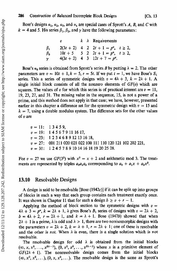
286 Construction of Balanced Incomplete Block Designs [Ch. 13
Bose's designs al , a2, a3 , and a4 are special cases of Sprott's A, B, and C withk = 4 and 5. His series P1i j2, and y have the following parameters:
k A Requirements
p1 2(3t + 2) 4 2 2t + 1 = p", t >- 2,fla 10t + 5 5 2 2t+1=p", t>-2,y 4(3t + 2) 4 3 12t + 7 =pa
Bose's a3 series is obtained from Sprott's series B by putting A = 2. The otherparameters are v = 10t + 1, k = 5, r = 5t. If we put t = 1, we have Bose's Sl
series. This a series of symmetric designs with v = 4X + 3, k = 2A + 1. Asingle initial block consists of all the nonzero elements of GF(v) which aresquares. The values of v for which this series is of practical interest are v = 11,19, 23, 27, and 31. The missing value in the sequence, 15, is not a power of aprime, and this method does not apply in that case; we have, however, presentedearlier in this chapter a difference set for the symmetric design with v = 15 andk = 7, using a double modulus system. The difference sets for the other valuesof v are
v=11: 13459,v=19: 145679111617,v=23: 1 234689 1213 16 18,v = 27: 001 211 020 021 022 100 111 110 120 121 102 202 221,v = 31: 1 24578910141618 19202528.
For v = 27 we use GF(3 3) with x3 = x + 2 and arithmetic mod 3. The treat-ments are represented by triples aoa1a2 corresponding to ao + alx + a2x2 .
13.10 Resolvable Designs
A design is said to be resolvable [Bose (1942c)] if it can be split up into groupsof blocks in such a way that each group contains each treatment exactly once.It was shown in Chapter 11 that for such a design b >_ v + r - 1.
Applying the method of block section to the symmetric designs with v =4A + 3 = p", k = 2,1 + 1, A gives Bose's Bl series of designs with v = 2a + 2,b = 4a + 2, r = 2A + 1, and k = A + 1. Bose (1947b) showed that when2,1 + 1 is a prime, A is odd and ,\ > 1, there are two nonisomorphic designs withthe parameters v = 2,1 + 2, k = A + 1, r = 2,1 + 1; one of these is resolvableand the other is not. When A is even, there is a single solution which is notresolvable.
The resolvable design for odd ,1 is obtained from the initial blocks(cc x x3 x211-1) (0 x° xa x211-1) where x is a primitive element ofGF(2,1 + 1). The nonresolvable design comes from the initial blocks(cc, x°, x2, ... ), (0, x, x3,.. . ). The resolvable design is the same as Sprott's
Dow
nloa
ded
12/1
1/12
to 1
29.1
28.2
07.2
42. R
edis
trib
utio
n su
bjec
t to
SIA
M li
cens
e or
cop
yrig
ht; s
ee h
ttp://
ww
w.s
iam
.org
/jour
nals
/ojs
a.ph
p

Exercises 287
series 4 design, and it has the additional property that all triples of treatmentsoccur the same number of times. The design with A = 3 has v = 8, b = 14,r = 7, and k = 4. It is
00356, co460, 00501, co612, co023, co134, co245,0124, 1235, 2346, 3450, 4561, 5602, 6013.
Sprott's series 5 designs are also resolvable designs with the property thatevery triple occurs the same number of times. They have v = 2k, b = 4(2k - 1),r = 2(2k - 1), A = 2(k - 1), and it is necessary that 2k - 1 = p". The designis obtained from the four initial blocks
(0, x, (cc x11, x{+ 3 x{ +2k-3) l = 0 1.
The doubly balanced designs of Calvin (1954) are special cases of these series.
Exercises
1. Show that the complement of a BIBD is also a BIBD.2. Show that the existence of a design with v = n2, k = n, and A = 1 implies the
existence of a complete set of orthogonal Latin squares of side n. Hence thereexists no design with v = 36, k = 6, and ,1 = 1.
3. Show that the equation
x2 = 6y2 + 5z2
has no solution in integers other than the trivial solution x = y = z = 0.4. If v is a prime and v = 4t + 3, show that the quadratic residues of v form a
perfect difference set.5. (Continuation). Show that if v = 27, and if the varieties are represented by
elements of GF(3 3), the quadratic residues also form a difference set. That is theexample given in the text.
6. We stated in the discussion of Sprott's series D that if the necessary requirementis violated by any primitive x, it is violated by all primitive elements. Prove this.
7. Show that the differences are symmetrically repeated in Bose's resolvable B1
designs.8. Find counterexamples to show the following:
(i) The equality b = v + r - 1 does not ensure that v = nk where n is aninteger;
(ii) v = nk is not sufficient to ensure resolvability.
9. Show that for an affine resolvable design (i.e., a design with b = v + r - 1) theparameters can be written as
v = n2((n - 1)t + 1), b = n(n2t + n + 1), k = n((n - 1)t + 1),
r=n2t+n+1, a =nt+1.
Dow
nloa
ded
12/1
1/12
to 1
29.1
28.2
07.2
42. R
edis
trib
utio
n su
bjec
t to
SIA
M li
cens
e or
cop
yrig
ht; s
ee h
ttp://
ww
w.s
iam
.org
/jour
nals
/ojs
a.ph
p

CHAPTER 14
The Existence andConstruction of
Partially BalancedDesigns
In Chapter 12 we initiated our discussion of partially balanced associationschemes and partially balanced designs. These were introduced in 1939 by Boseand Nair because of the restrictions on the existence of balanced incompleteblock designs, especially in the case where v — 1 is a prime. We have postponeduntil now the discussion of the existence and construction of designs with theseveral association schemes. This chapter, like Chapter 13, is of more mathema-tical interest than the others. The reader who does not wish to work his waythrough it may find a design to fit his requirements by using the tables of designsassembled by Bose, Clatworthy, and Shrikhande (1954), and by Clatworthy(1956).
We shall present in the next section some elementary designs that can beobtained from any association scheme. In the subsequent sections we shall,for the most part, confine our attentions to partially balanced designs with onlytwo associate classes, and present methods of obtaining designs with the groupdivisible, triangular, and Latin square association schemes. Even for theseschemes there are still some sets of parameters with k < 10 and r < 10 forwhich it is not known whether or not a design exists. The eighteen unsolvedcases for the triangular scheme and the five unsolved cases for the L2 scheme arelisted in the relevant sections of the chapter. More problems of interest remainto be solved for PBIB(m) designs with m > 2.
The reader will wish to refer to Chapter 12 for the introductory remarks aboutpartially balanced designs. He will then recall that we begin with a partiallybalanced association scheme. A PBIB design with that scheme is then anequireplicate, proper, binary design, i.e., a design in which the treatments eachappear r times in blocks of k plots each, with no treatment appearing more than
288
Dow
nloa
ded
12/1
1/12
to 1
29.1
28.2
07.2
42. R
edis
trib
utio
n su
bjec
t to
SIA
M li
cens
e or
cop
yrig
ht; s
ee h
ttp://
ww
w.s
iam
.org
/jour
nals
/ojs
a.ph
p

The Existence and Construction of Partially Balanced Designs 289
once in any block. Each pair of ith associates appears together in exactly A i
blocks. The A { need not all be different.We have already given a proof in Chapter 11 of Kempthorne's conjecture
that, of all proper, binary, equireplicate designs with a given set of parameters(b, v, r, k), the balanced incomplete block design, if it exists, is the most efficient.The experimenter wil] usually not, therefore, choose a partially balanced designin preference to a balanced design, nor, if the blocks are large enough, will hechoose an incomplete block design over the randomized complete block design.The efficiency of an incomplete block design has been shown (Chapter 11) to begiven by N - lv8 where S is the harmonie mean of the nonzero latent roots of thematrix A of the reduced intrablock equations.
Let N be the incidence matrix of a partially balanced design. We shall show inChapter 15 that if 0 is a latent root of NN' with multiplicity a, then
O j = (rk — 9 t)^k
is a root of A with the same multiplicity a { . For every connected design NN' has aroot 0 = rk with ao = 1. It is only meaningful to talk about efficiency forconnected designs, in which case
E= (v — 1)I(r ajoi 1).
The largest value of E that can be hoped for with v varieties in blocks of size kis
E = (dv)/(rk)
where it(v — 1) = r(k — 1), i.e.,
v(k-1) v—kEmax = k(v-1)
-1—k(v— 1)
.
For any design the parameters r, k, n i , and ,1, must satisfy the equation
r(k — 1) _ ,lint .
Furthermore, since NN' is a nonnegative definite matrix, its roots 0 must all benonnegative. We shall see in Chapter 15 that for a PBIB(m) design there are,other than the simple root 0 = rk, only m distinct roots 9; ; their values and thevalues of the multiplicities a are readily obtained by the methods to be given inthat chapter. This provides us with a convenient method of establishing thenonexistence of designs with some sets of parameters. In addition, for asymmetric design the determinant INN'1 is a square and so rk0i10z2... is asquare. Thus, for example, if all the roots are positive and if «• is even for alli, i > 1, but al is odd, then 0 must be a perfect square. This is, of course, anextension of the method that we used earlier to show that in a symmetric balancedincomplete block design with v even, (r — a) must be a square.
Dow
nloa
ded
12/1
1/12
to 1
29.1
28.2
07.2
42. R
edis
trib
utio
n su
bjec
t to
SIA
M li
cens
e or
cop
yrig
ht; s
ee h
ttp://
ww
w.s
iam
.org
/jour
nals
/ojs
a.ph
p

290 The Existence and Construction of Partially Balanced Designs [Ch. 14
For some association schemes, other conditions for the nonexistence ofsymmetric designs have been derived. These conditions make use of the Hilbertsymbol (a, b), and depend upon the Hasse—Minkowski invariant. Because thecalculation of these invariants is usually quite tedious, we shall content ourselvesby giving references where needed to the appropriate papers. The latent roots ofNN' are also of importance in linked block designs.
14.1 Duality and Linked Block Designs
The concept of duality comes from projective geometry in which it is possibleto obtain from one theorem a second one by interchanging in the statement suchwords as line and point. The statements "There is one straight line common toany two points" and "There is one point common to any two lines" are duals.In the present context, the dual design is obtained by interchanging blocks andvarieties.
Consider the unreduced BIBD with v* = 4, k* = 2. The parameters arev* = 4, b* = 6, k* = 2, r* = 3, and A* = 1; the design is AB, AC, AD, BC,BD, CD.
In the dual the varieties are a, b, c, d, e, f, corresponding to the six originalblocks. The statement "Variety A appears in blocks 1, 2, and 3" becomes"Block 1 contains the varieties a, b, and c." This gives the new design abc; ade;bdf; cef with parameters v = b* = 6, b = v* = 4, k = r* = 3, and r = k* = 2.The dual design is actually a triangular PBIB(2) design. It does not, however,follow that the dual of a balanced incomplete block design is always a PBIB(2)design. This will be discussed further in Chapter 14.
Youden (1951) defined linked block designs as designs with the property thateach pair of blocks has the same number (p) of varieties in common. It followsthat the dual has the property that each pair of varieties has the same number (µ)of blocks in common, i.e., the dual is a balanced incomplete block design.If µ = 1, we have singly linked blocks; if µ = 2, we have doubly linked blocks.The main properties of linked block designs are given by J. Roy and Laha(1957a,b).
Let NN' be the interblock matrix for a linked block design; N'N is the inter-block matrix for the dual (BIBD). We recall that if A and B are matricessuch that AB and BA both exist, then AB and BA have the same nonzero latentroots. Thus NN' has the same nonzero latent roots as N'N, namely r*k* andr*(v* — k*)/(v* — 1) = r* — A*. Furthermore, NN' and N'N have the samerank and the same trace. This leads to the following result, due to J. Roy andLaha (1957b).
A necessary and sufficient condition that a design be a linked block design isthat NN' has only one nonzero latent root other than rk, namely,
_ k(b—r)e b-1
and the multiplicity of 0 is a = b — 1.
Dow
nloa
ded
12/1
1/12
to 1
29.1
28.2
07.2
42. R
edis
trib
utio
n su
bjec
t to
SIA
M li
cens
e or
cop
yrig
ht; s
ee h
ttp://
ww
w.s
iam
.org
/jour
nals
/ojs
a.ph
p
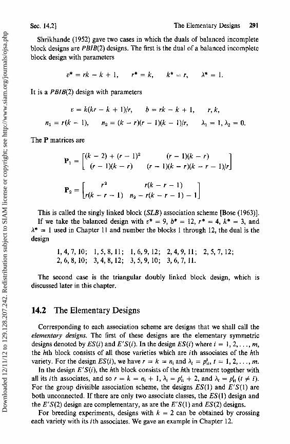
Sec. 14.2] The Elementary Designs 291
Shrikhande (1952) gave two cases in which the duals of balanced incompleteblock designs are PBIB(2) designs. The first is the dual of a balanced incompleteblock design with parameters
v*=rk—k+l, r*=k, k*=r, A*=1.
It is a PBIB(2) design with parameters
v=k(kr—k+ 1)/r, b=rk—k+ 1, r,k,
n1 = r(k — 1), n2 = (k — r)(r — 1)(k — 1)/r, A l = 1, d2 = 0.
The P matrices are
P— —2)+(r-1)Z (r-1)(k—r)l [(k
(r — 1)(k — r) (r — 1)(k — r)(k - r — 1)/r]
_r 2 r(k—r— 1)
P^ — [r(k—r— 1) n2 —r(k—r— 1)— 1,
This is called the singly linked block (SLB) association scheme [Bose (1963)].If we take the balanced design with v* = 9, b* = 12, r * = 4, k* = 3, and
d* = 1 used in Chapter 11 and number the blocks 1 through 12, the dual is thedesign
1,4,7,10; 1,5,8,11; 1,6,9,12; 2,4,9,11; 2,5,7,12;2, 6, 8, 10; 3,4,8,12; 3,5,9,10; 3,6,7, 11.
The second case is the triangular doubly linked block design, which isdiscussed later in this chapter.
14.2 The Elementary Designs
Corresponding to each association scheme are designs that we shall call theelementary designs. The first of these designs are the elementary symmetricdesigns denoted by ES(i) and E'S(i). In the design ES(i) where i = 1, 2, ..., m,the hth block consists of all those varieties which are ith associates of the hthvariety. For the design ES(i), we have r = k = n, and At = p, t = 1, 2, ..., m.
In the design E'S(i), the hth block consists of the hth treatment together withall its ith associates, and so r = k = n, + 1, ,1s = pi ; + 2, and A t = p,, (t 0 i).For the group divisible association scheme, the designs ES(1) and E'S(l) areboth unconnected. If there are only two associate classes, the ES(l) design andthe E'S(2) design are complementary, as are the E'S(l) and ES(2) designs.
For breeding experiments, designs with k = 2 can be obtained by crossingeach variety with its ith associates. We gave an example in Chapter 12.
Dow
nloa
ded
12/1
1/12
to 1
29.1
28.2
07.2
42. R
edis
trib
utio
n su
bjec
t to
SIA
M li
cens
e or
cop
yrig
ht; s
ee h
ttp://
ww
w.s
iam
.org
/jour
nals
/ojs
a.ph
p

292 The Existence and Construction of Partially Balanced Designs [Ch. 14
We can also make up elementary designs by combining a collection of v BIBdesigns. The hth of these balanced designs is constructed from the set of ithassociates of the hth variety and has parameters b*, v* = ni, k*, r*, and A*. Thenwe have for the combined design b = vb*, k = k*, r = n (r*, and At = pi,a*. Ifwe now add the hth variety itself to each of the blocks in the hth BIBD, we havea design with b = vb*, k = k* + 1, r = n tr* + b*, Ai = 2r* + pA*, andk= PILA* (t0i).
14.3 Group Divisible Designs
This was the first association scheme to be investigated extensively. Contri-butions have been made by Bose and Connor (1952), Connor (1952b), Bose et al.(1953), and Freeman (1957). The matrix NN' has each diagonal element r; theoff-diagonal elements are either Al or '2 . For the GD design, if we order thevarieties by groups so that the first n varieties are in the first group, and so on,NN' consists of submatrices (r — a1)In + ) 1J the main diagonal andsubmatrices Mn off the diagonal. We can evaluate the determinant as =(r + (n — 1)A1 + (m — 1)nÁ2)(r — Á1 + n('\1 — ,\2))m-1(r — A1)m(n -1) Substi-tuting r — 0 for r we see that the latent roots and their multiplicities are
00 =r +(n— 1)Al +(m— 1)nd2 =rk, a0 =1;
B1 = r+,11(n— 1)—,\2n=rk—A2v, a1 = m — 1;
02 =r—Al , a2=m(n-1)
The latent roots and their multiplicities will be obtained more easily later. Forbinary designs we cannot have Al > r, and so the condition 0 2 >_ 0 is trivial.However, the condition 0 >_ 0 can be used to establish the nonexistence ofsome designs, as the following example shows.
Let m = 6 and n = 4. The condition r(k — 1) = l{ n iA becomes
r(k — 1) = (n — 1).\ + n(m — 1)A 2 .
A design with Al = 0, A2 = 11, r = 20, and k = 12 would satisfy this require-ment and also the requirement that b be an integer. However, 0 = 20 — 44 =— 24, and so no such design exists.
For symmetric designs, we note that the determinant
!NN ' I = r 2(r l — vÁ2)m -1(r — Á1)m(7-1)
must be a perfect square. If neither 0 nor 02 is zero, the following conditions arenecessary:
(i) If m is odd and n is even, then r — ,11 must be a square;(ii) If m is even, then r 2 — v)t2 is a square.
Dow
nloa
ded
12/1
1/12
to 1
29.1
28.2
07.2
42. R
edis
trib
utio
n su
bjec
t to
SIA
M li
cens
e or
cop
yrig
ht; s
ee h
ttp://
ww
w.s
iam
.org
/jour
nals
/ojs
a.ph
p

Sec. 14.5] Semiregular Designs 293
Thus, for example, condition (i) rules out the design for v = b = 22, r = k = 5,m = 11, n = 2, t = 0, and A2 = 1; condition (ii) rules out v = b = 44,r = k = 7, m = 22, n = 2, A, = 0, and A2 = 1. Bose and Connor (1952) haveextended these results, using the Hasse—Minkowski invariant. Bose and Connor(1952) divided the GD designs into three classes which are mutually exclusive:
(i) Singular designs, which are designs for which 02 = 0, i.e., r = a l ;(ii) Semiregular designs which have 0 1 = 0, 62 > 0;
(iii) Regular designs which have 9 1 > 0, 02 > 0.
If both 0 and 02 are zero, we have the complete block design with b = r andk = v.
14.4 Singular Designs
For a design with r = A l , the varieties have to occur by groups. Whenever agiven variety appears in a block, all varieties in the same group must also appearin that block. The simplest example is the design with b = m, k = n, and r = 1,in which each block consists of a single group of varieties. The E'S(1) designrepeats this design n timer. The ES(2) design is also singular.
Singular designs with t2 > 0 are obtained from balanced incomplete blockdesigns. If we take a balanced design with parameters v* = m, b*, r*, k*, and A*,and replace each treatment by a group of n varieties, we obtain a singular GDdesign with v = mn, b = b*, r = d l = r *, k = nk*, and A2 = A*. Indeed, everysingular GD design with A l = 0 can be obtained by this method. It is possibleto have b < v, as we saw in the preceding paragraph, because the rank of NN' is1 + a i = m. The inequality b >_ v, which holds for balanced incomplete blockdesigns, is thus replaced by b >_ m.
Zelen (1954) points out that this method of replacing each variety by a groupof n new varieties can be used to derive a PBIB(m + 1) design from anyPBIB(m) design, and P. M. Roy (1953) has incorporated this idea into hishierarchical GD designs.
14.5 Semiregular Designs
Bose and Connor (1952) prove the following theorem.
Theorem. A necessary and sufficient condition for a group divisible design to be semi-regular is that k = cm where c is an integer, and that each block contain exactly cvarieties from each of the groups.
PROOF. Suppose that we have a GD design with parameters v = mn, r, k, ,1 1 , andAl.
Dow
nloa
ded
12/1
1/12
to 1
29.1
28.2
07.2
42. R
edis
trib
utio
n su
bjec
t to
SIA
M li
cens
e or
cop
yrig
ht; s
ee h
ttp://
ww
w.s
iam
.org
/jour
nals
/ojs
a.ph
p

294 The Existence and Construction of Partially Balanced Designs [Ch. 14
Sufficiency: Consider a variety in the jth group. It appears r times, and on eachoccasion there are, in the same block, c varieties from the hth group, (h 0 j).Then
rc = ÁZn.
We also have k = cm so that
rk=rcm=mn 2 =A2v,
and the design is semiregular.
Necessity: Suppose that the design is semiregular and that the jth block con-tains ef varieties belonging to the first group. Then ef = nr.
The jth block contains (2) pairs of varieties from the first group. Each of
these pairs of varieties occurs together in A l blocks, and so
6
^ej(ef -1)=Aln(n-1).
It follows that
1 ei = n(n — 1)i\ + nr = n(rk — n(m — 1)A2) = n2A2 .
Let é = nr/b = vr/(mb) = k/m = c. Then b (e, — é)2 = n2b 2 — n2r2 = 0,and e l = e2 = • • • = em = é = c. But ej is an integer and so c is an integer.The same argument applies for each group of varieties, and so each blockcontains exactly c varieties from each group. u
It is easily shown that for a semiregular GD design b >_ v — m + 1. Fromany semiregular design with v = mn treatments, a design with parametersv* = m in, b, r, k* = cml, A1, A2 may be obtained by cutting out (m — m l) ofthe groups of treatments.
When Bose (1942c) established the inequality
b>v+r-1
for resolvable balanced incomplete block designs, he called affine resolvablethose designs for which the equality b = v + r — 1 held. He showed that for anaffine resolvable design with v = nk, each block in a given replication has exactlyk/n varieties in common with each of the blocks in every other replication; kin isan integer.
It follows that the dual of an affine resolvable balanced incomplete blockdesign is a semiregular GD design. When we take the dual, blocks that were inthe same replication become varieties in the same group, and, since the blocks inany replication are disjoint, we have A l = 0. Since blocks in different replications
Dow
nloa
ded
12/1
1/12
to 1
29.1
28.2
07.2
42. R
edis
trib
utio
n su
bjec
t to
SIA
M li
cens
e or
cop
yrig
ht; s
ee h
ttp://
ww
w.s
iam
.org
/jour
nals
/ojs
a.ph
p
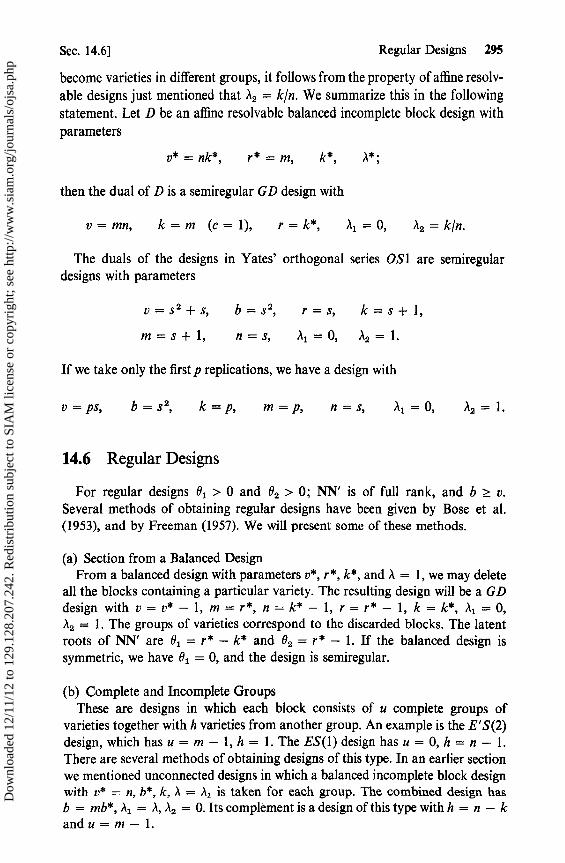
Sec. 14.6] Regular Designs 295
become varieties in different groups, it follows from the property of affine resolv-able designs just mentioned that A2 = kin. We summarize this in the followingstatement. Let D be an affine resolvable balanced incomplete block design withparameters
v* = nk*, r* = m, k*, A*;
then the dual of D is a semiregular GD design with
v = mn, k = m (c = 1), r = k*, a1 =0, A2 =kin.
The duals of the designs in Yates' orthogonal series OS1 are semiregulardesigns with parameters
v=sa+s, b=s 2 , r=s, k=s+1,
m=s+1, n=s, A=0, A2 =1.
If we take only the first p replications, we have a design with
v=ps, b=s 2, k=p, m=p, n=s, Al =0, A.=1.
14.6 Regular Designs
For regular designs 0 > 0 and 0 2 > 0; NN' is of full rank, and b >_ v.Several methods of obtaining regular designs have been given by Bose et al.(1953), and by Freeman (1957). We will present some of these methods.
(a) Section from a Balanced DesignFrom a balanced design with parameters v*, r*, k*, and ,1 = 1, we may delete
all the blocks containing a particular variety. The resulting design will be a GDdesign with v=v* — 1, m=r*, n=k* — 1, r=r* — 1, k=k*, X1 1 =0,a2 = 1. The groups of varieties correspond to the discarded blocks. The latentroots of NN' are 01 = r* — k* and 02 = r* — 1. If the balanced design issymmetric, we have 9 1 = 0, and the design is semiregular.
(b) Complete and Incomplete GroupsThese are designs in which each block consists of u complete groups of
varieties together with h varieties from another group. An example is the E'S(2)design, which has u = m — 1, h = 1. The ES(1) design has u = 0, h = n — 1.There are several methods of obtaining designs of this type. In an earlier sectionwe mentioned unconnected designs in which a balanced incomplete block designwith v* = n, b*, k, A = al is taken for each group. The combined design hasb = mb*, A, = A, ,l2 = 0. Its complement is a design of this type with h = n — kand u =m-1.
Dow
nloa
ded
12/1
1/12
to 1
29.1
28.2
07.2
42. R
edis
trib
utio
n su
bjec
t to
SIA
M li
cens
e or
cop
yrig
ht; s
ee h
ttp://
ww
w.s
iam
.org
/jour
nals
/ojs
a.ph
p
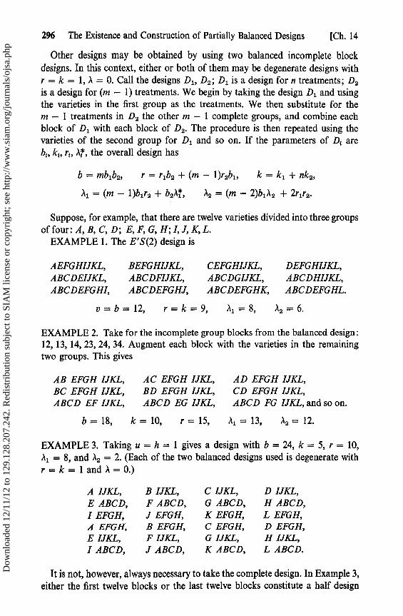
296 The Existence and Construction of Partially Balanced Designs [Ch. 14
Other designs may be obtained by using two balanced incomplete blockdesigns. In this context, either or both of them may be degenerate designs withr = k = 1, A = 0. Call the designs D l , D2 ; D l is a design for n treatments; D2
is a design for (m — 1) treatments. We begin by taking the design Dl and usingthe varieties in the first group as the treatments. We then substitute for them — 1 treatments in Da the other m — 1 complete groups, and combine eachblock of Dl with each block of D2 . The procedure is then repeated using thevarieties of the second group for D l and so on. If the parameters of D{ arebi, k,, r1, A*, the overall design has
b = mb1b2 , r = r1b2 + (m — 1)r2b1 , k = k l + nk2 ,
Al = (m — 1)b1r2 + b2 Ai, A2 = (m — 2)b 1 A 2 + 2r1r2 .
Suppose, for example, that there are twelve varieties divided into three groupsoffour:A,B,C,D; E, F, G, H; I, J, K, L.
EXAMPLE 1. The E'S(2) design is
AEFGHIJKL, BEFGHIJKL, CEFGHIJKL, DEFGHIJKL,ABCDEIJKL, ABCDFIJKL, ABCDGIJKL, ABCDHIJKL,ABCDEFGHI, ABCDEFGHJ, ABCDEFGHK, ABCDEFGHL.
v =b =12, r =k =9, Al =8, ,12 =6.
EXAMPLE 2. Take for the incomplete group blocks from the balanced design:12, 13, 14, 23, 24, 34. Augment each block with the varieties in the remainingtwo groups. This gives
AB EFGH IJKL, AC EFGH IJKL, AD EFGH IJKL,BC EFGH IJKL, BD EFGH IJKL, CD EFGH IJKL,ABCD EF IJKL, ABCD EG IJKL, ABCD FG IJKL, and so on.
b = 18, k = 10, r = 15, Al = 13, a2 = 12.
EXAMPLE 3. Taking u = h = 1 gives a design with b = 24, k = 5, r = 10,dl = 8, and ' 2 = 2. (Each of the two balanced designs used is degenerate withr = k = 1 and A = 0.)
A IJKL, B IJKL, C IJKL, D IJKL,E ABCD, F ABCD, G ABCD, H ABCD,I EFGH, J EFGH, K EFGH, L EFGH,A EFGH, B EFGH, C EFGH, D EFGH,E IJKL, F IJKL, G IJKL, H IJKL,I ABCD, J ABCD, K ABCD, L ABCD.
It is not, however, always necessary to take the complete design. In Example 3,either the first twelve blocks or the last twelve blocks constitute a half design
Dow
nloa
ded
12/1
1/12
to 1
29.1
28.2
07.2
42. R
edis
trib
utio
n su
bjec
t to
SIA
M li
cens
e or
cop
yrig
ht; s
ee h
ttp://
ww
w.s
iam
.org
/jour
nals
/ojs
a.ph
p
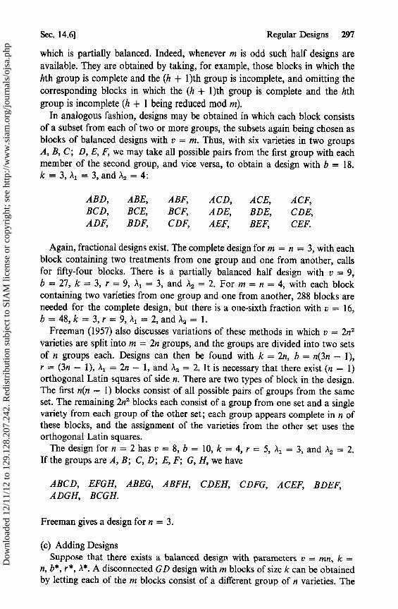
Sec. 14.6] Regular Designs 297
which is partially balanced. Indeed, whenever m is odd such half designs areavailable. They are obtained by taking, for example, those blocks in which thehth group is complete and the (h + 1)th group is incomplete, and omitting thecorresponding blocks in which the (h + 1)th group is complete and the hthgroup is incomplete (h + 1 being reduced mod m).
In analogous fashion, designs may be obtained in which each block consistsof a subset from each of two or more groups, the subsets again being chosen asblocks of balanced designs with v = m. Thus, with six varieties in two groupsA, B, C; D, E, F, we may take all possible pairs from the first group with eachmember of the second group, and vice versa, to obtain a design with b = 18.k = 3, A1 = 3, and A2 =4:
ABD, ABE, ABF, ACD, ACE, ACF,BCD, BCE, BCF, ADE, BDE, CDE,ADF, BDF, CDF, AEF, BEF, CEF.
Again, fractional designs exist. The complete design for m = n = 3, with eachblock containing two treatments from one group and one from another, callsfor fifty-four blocks. There is a partially balanced half design with v = 9,b = 27, k = 3, r = 9, Al = 3, and A2 = 2. For m = n = 4, with each blockcontaining two varieties from one group and one from another, 288 blocks areneeded for the complete design, but there is a one-sixth fraction with v = 16,b = 48,k = 3,r = 9, Al = 2,andA2 = 1.
Freeman (1957) also discusses variations of these methods in which v = 2n2
varieties are split into m = 2n groups, and the groups are divided into two setsof n groups each. Designs can then be found with k = 2n, b = n(3n — 1),r = (3n — 1), Al = 2n — 1, and A2 = 2. It is necessary that there exist (n — 1)orthogonal Latin squares of side n. There are two types of block in the design.The first n(n — 1) blocks consist of all possible pairs of groups from the sameset. The remaining 2n2 blocks each consist of a group from one set and a singlevariety from each group of the other set; each group appears complete in n ofthese blocks, and the assignment of the varieties from the other set uses theorthogonal Latin squares.
The design for n = 2 has v = 8, b = 10,k=4,r=5,1 1 =3, and ,12 =2.If the groups are A, B; C, D; E, F; G, H, we have
ABCD, EFGH, ABEG, ABFH, CDEH, CDFG, ACEF, BDEF,ADGH, BCGH.
Freeman gives a design for n = 3.
(c) Adding DesignsSuppose that there exists a balanced design with parameters v = mn, k =
n, b*, r*, A*. A disconnected GD design with m blocks of size k can be obtainedby letting each of the m blocks consist of a different group of n varieties. The
Dow
nloa
ded
12/1
1/12
to 1
29.1
28.2
07.2
42. R
edis
trib
utio
n su
bjec
t to
SIA
M li
cens
e or
cop
yrig
ht; s
ee h
ttp://
ww
w.s
iam
.org
/jour
nals
/ojs
a.ph
p

298 The Existence and Construction of Partially Balanced Designs [Ch. 14
design obtained by repeating the balanced design s times and then repeating thedisconnected design t times is a regular GD design with parameters
v=mn, b=b*s+mt, k=n, r=r*s+t,
Al = A*s + t, Á2 = Á*s.
Adesignforv=9,m=3,n=3,b=27,k=3,a 1 =3,andA2 =2hasjust been mentioned; each block contained two varieties from one group andone from another. Bose, Clatworthy, and Shrikhande (1954) give a different(nonisomorphic) design with the same parameters. They repeat the orthogonalseries design with v = k2 = 9 and b = 12 twice, and then repeat one of thesquares a third time, which amounts to taking s = 2 and t = 1.
In the previous example of adding a disconnected design to a balanced designit happend that the balanced design was resolvable and that the disconnecteddesign comprised one of the replications in it. Bose et al. (1953) use a method ofrepeating a resolvable balanced incomplete block design t times and furtherrepeating one of the replicates an additional a times where a may be positive(addition) or negative (subtraction).
Other designs may be obtained by adding partially balanced designs tobalanced designs. We have mentioned Freeman's design for v = 16, m = n = 4,b = 48, k = 3, A l = 2, and A2 = 1. A nonisomorphic design is found in theBose, Clatworthy, and Shrikhande tables, design R38 (1954). It may be con-structed from other designs in the following way. We first take for each groupthe BIBD for v = b = 4, r = k = 3, and A = 2. These sixteen blocks are adesign with A l = 2 and X12 = 0, and we add to them design R35 of Bose et al.(1954), which has v = 16, m = n = 4, k = 3, Al = 0, and '2 = 1. Otherexamples of this method are given by Bose et al. (1953).
This method of adding designs is not confined in its application to groupdivisible schemes. If in the general case we can find designs D{ of block size kwith the property that A, = 1 and Ah = 0 for all h 0 i, we can easily construct adesign of block size k for any set of parameters A l , A2, ... by repeating eachbasic design Di exactly A, times. An example will be found in the section onLatin square designs.
(d) Extension of DesignsIt will be recalled that the complete lattice design with v = k2 = 9, b = 12,
r = 4, and A = 1 is resolvable and can be made into a balanced design forv = b = 13 and r = k = 4 in the following way. A new block is added con-taining the four new variaties, a plot with the first new variety is added to eachblock in the first replicate, the second new variety is added to each block in thesecond replicate, and so on. This method of adding r additional varieties to makea design with block size k + 1 has its parallel in the construction of GD designs.Suppose that there exists a resolvable GD design with parameters v = mn = ks,b = rs, r, k, Al , A2 = 1, and also that there exists another GD design with
Dow
nloa
ded
12/1
1/12
to 1
29.1
28.2
07.2
42. R
edis
trib
utio
n su
bjec
t to
SIA
M li
cens
e or
cop
yrig
ht; s
ee h
ttp://
ww
w.s
iam
.org
/jour
nals
/ojs
a.ph
p

Sec. 14.6] Regular Designs 299
parameters v' = r = m'n, b', r' = r — s, k' = k + 1, A, = Al, and X = 1where m' is an integer; then we may allocate one new variety to each replicatein the first design, adding it to each block in the replicate, and obtain a new GDdesign with parameters
v= v+v'=v +r, b=b+b', P=r, kC=k+1,
rn = m + m ' , n = n, nl = A1, "2 = 1 .
There is a paucity of examples of moderate size. The following one is found inthe paper by Bose et al. (1953).
EXAMPLE. A resolvable GD design for v = 6 and k = 2 is obtained by taking
the unreduced design with b = () = 15 and repeating one of the replicates.
This gives a design with v = 6, b = 18, r = 6, k = 2, m = 3, n = 2, A l = 2, andA2 = 1:
AB, CD, EF; AB, CD, EF; AC, BE, DF; AD, BF, CE; AE, BD, CF;AF, BC, DE.
A design for v'= r=6,k'=k+1=3,m=3,n =2, A 1 = 2, and A2 =1is
UWX, VWX, WYZ, XYZ, UVY, UVZ.
The combined design with v = 12, b = 24, r" = 6, k = 3, m = 6, n = 2,.1 1 = 2, and ,C2 = 1 is
ABU, CDU, EFU, ABV, CDV, EFV, ACW, BEW,DFW, ADX, BFX, CEX, AEY, BDY, CFY, AFZ,BCZ, DEZ, UWX, VWX, WYZ, XYZ, UVY, UVZ.
(e) Difference SetsWe quote without proof the following theorem of Bose et al. (1953), which is
similar to Bose's fundamental theorems for balanced incomplete block designs.
Theorem. Let M be a module with m elements and let n treatments correspond toeach element. Suppose that we can find a set of t initial blocks B i , B2,.. ., Bt eachof size k, and an initial group G of n elements, such that
(i) The n(n — 1) differences (reduced mod m) arisingErom G are all different,and
(ii) Among the k(k — 1)t differences occurring in the initial blocks, eachdifferente occurs t2 times, except those that arise in G, which each occur ,1 1
times.
Dow
nloa
ded
12/1
1/12
to 1
29.1
28.2
07.2
42. R
edis
trib
utio
n su
bjec
t to
SIA
M li
cens
e or
cop
yrig
ht; s
ee h
ttp://
ww
w.s
iam
.org
/jour
nals
/ojs
a.ph
p

300 The Existence and Construction of Partially Balanced Designs [Ch. 14
Then a GD design is obtained by cycling (mod m) from the initial blocks B 1 ,
B2, ... , B.
EXAMPLE. v = b = 14, m = 7, n = 2, Al = 0, and A2 = 1. There are twoinitial blocks (1 1 , 21 , 41 , 02), (1 2, 22 , 42 , 0 1). We denote the jth variety in the ithgroup by i; , 0 < i <_ m - 1, 0 < j < n - 1. Arithmetic is mod 7. The initialgroup is 01 , 02 . In the differences [1, 1] each value 1, 2, ..., 6 occurs once; thesame is true for the differences [2, 2]. In the differences [1, 2] and again in thedifferences [2, 1], each value 0, 1, 2, ... , 6 occurs once, except for zero, whichdoes not appear. In the initial group there are no differences [1, 1] or [2, 2]; theonly difference [1, 2] or [2, 1] is zero. Thus, the conditions of the theorem aresatisfied and we have the following design:
1 1 21 41 02, 21 31 51 1 2, 31 41 6 1 22, 41 51 01 32,5161 1 1 42, 61 01 21 52, 01 1 1 3 1 62 ,
12 22 42 01, 22 32 52 1 1, 32 42 62 21, 42 52 02 31,52 62 12 41, 62 02 22 51, 02 1 2 3 2 61.
Again, it is sometimes possible to find fractional or partial designs, and theprevious theorem can be generalized.
Let M be a module with cm elements and let n jc (an integer) varieties corre-spond to each element of M. Suppose that we can find a set of t initial blocks of ktreatments each and an initial group G of n treatments such that
(i) The differences arising from G take n(n - 1)1c different values, each ofwhich is repeated c times, the values being equally spaced;
(ii) Among the kt(k - 1) differences in the initial blocks, each value occurs A 2
times, except for those occurring in G, which occur A l times each.
Then, developing the initial blocks gives a GD design with parametersv = mn, b = met, r = kct/n, m, n, X11, Az.
EXAMPLE. v = b = 12, r = k = 4, m = 6, n = 2, l = 2, A2 = 1. Initialblock 0, 1, 4, 6; initial group (0, 6); c = 2. The design is
0146, 347 9, 67100, 91013,
1257, 45810, 78111, 101124,
2368, 56911, 89 02, 11 035.
(f) Designs Based on Projective GeometriesSome designs based on finite geometries are given in the original paper by
Bose and Nair (1939). We give an illustrative example here.In the Euclidean geometry with N = 2, consider only lines that do not pass
through the origin. Then lines are blocks, points are treatments, and we have a
Dow
nloa
ded
12/1
1/12
to 1
29.1
28.2
07.2
42. R
edis
trib
utio
n su
bjec
t to
SIA
M li
cens
e or
cop
yrig
ht; s
ee h
ttp://
ww
w.s
iam
.org
/jour
nals
/ojs
a.ph
p
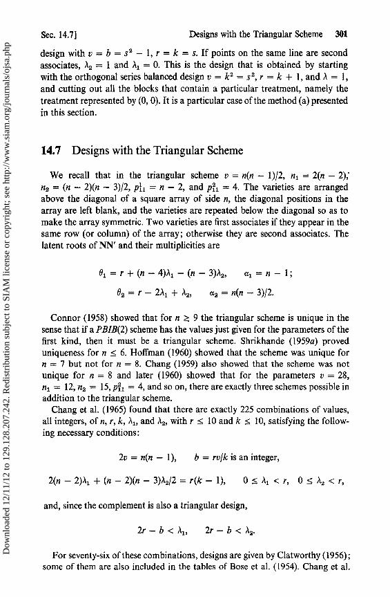
Sec. 14.71 Designs with the Triangular Scheme 301
design with v = b = s 2 — 1, r = k = s. If points on the same line are secondassociates, A2 = 1 and Al = 0. This is the design that is obtained by startingwith the orthogonal series balanced design v = k2 = s 2, r = k + 1, and ,\ = 1,and cutting out all the blocks that contain a particular treatment, namely thetreatment represented by (0, 0). It is a particular case of the method (a) presentedin this section.
14.7 Designs with the Triangular Scheme
We recall that in the triangular scheme v = n(n — 1)/2, n l = 2(n — 2);na = (n — 2)(n — 3)/2, pi l = n — 2, and pi l = 4. The varieties are arrangedabove the diagonal of a square array of side n, the diagonal positions in thearray are left blank, and the varieties are repeated below the diagonal so as tomake the array symmetric. Two varieties are first associates if they appear in thesame row (or column) of the array; otherwise they are second associates. Thelatent roots of NN' and their multiplicities are
B1 =r+(n-4)A,—(n-3)A2 , a1 =n— 1;
9 2 =r-2A1 + A2, a2 = n(n —3)/2.
Connor (1958) showed that for n >_ 9 the triangular scheme is unique in thelense that if a PBIB(2) scheme has the values just given for the parameters of thefirst kind, then it must be a triangular scheme. Shrikhande (1959a) proveduniqueness for n < 6. Hoffman (1960) showed that the scheme was unique forn = 7 but not for n = 8. Chang (1959) also showed that the scheme was notunique for n = 8 and later (1960) showed that for the parameters v = 28,nl = 12, n2 = 15, pil = 4, and so on, there are exactly three schemes possible inaddition to the triangular scheme.
Chang et al. (1965) found that there are exactly 225 combinations of values,all integers, of n, r, k, A l , and A2i with r < 10 and k < 10, satisfying the follow-ing necessary conditions:
2v = n(n — 1), b = rv/k is an integer,
2(n-2)Al +(n-2)(n-3)A2/2=r(k— 1), 0<Al <r, 0<A,<r,
and, sine the complement is also a triangular design,
2r—b< 1 , 2r—b< 2 .
For seventy-six of these combinations, designs are given by Clatworthy (1956);some of them are also included in the tables of Bose et al. (1954). Chang et al.
Dow
nloa
ded
12/1
1/12
to 1
29.1
28.2
07.2
42. R
edis
trib
utio
n su
bjec
t to
SIA
M li
cens
e or
cop
yrig
ht; s
ee h
ttp://
ww
w.s
iam
.org
/jour
nals
/ojs
a.ph
p
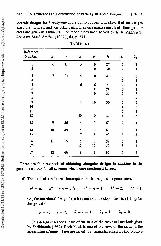
302 The Existence and Construction of Partially Balanced Designs [Ch. 14
provide designs for twenty-one more combinations and show that no designsexist in a hundred and ten other cases. Eighteen remain unsolved: their param-eters are given in Table 14.1. Number 7 has been solved by K. R. Aggarwal.See Ann. Math. Statist. (1972), 43, p. 371.
TABLE 14.1
ReferenceNumber n v k r b ,11 ,la
1 6 15 5 9 27 3 22 10 30 2 4
3 7 21 5 10 42 1 34 3 15 6 6 21 2 16 8 28 3 17 10 35 2 38 3 29 7 10 30 2 4
10 4 211 5 112 10 10 21 4 5
13 9 36 4 7 63 0 1
14 10 45 5 7 63 0 115 9 9 45 1 2
16 11 55 5 9 99 0 117 10 10 55 3 1
18 12 66 6 9 99 0 1
There are four methods of obtaining triangular designs in addition to thegeneral methods for all schemes which were mentioned before.
(i) The dual of a balanced incomplete block design with parameters
v*=n, b*=n(n-1)J2, r*=n-1, k*=2, A*,
i.e., the unreduced design for n treatments in blocks of two, is a triangulardesign with
b=n, r =2, k=n-1, a1 =1, I'2 =0.
This design is a special case of the first of the two dual methods givenby Shrikhande (1952). Each block is one of the rows of the array in theassociation scheme. These are called the triangular singly linked blocked
Dow
nloa
ded
12/1
1/12
to 1
29.1
28.2
07.2
42. R
edis
trib
utio
n su
bjec
t to
SIA
M li
cens
e or
cop
yrig
ht; s
ee h
ttp://
ww
w.s
iam
.org
/jour
nals
/ojs
a.ph
p
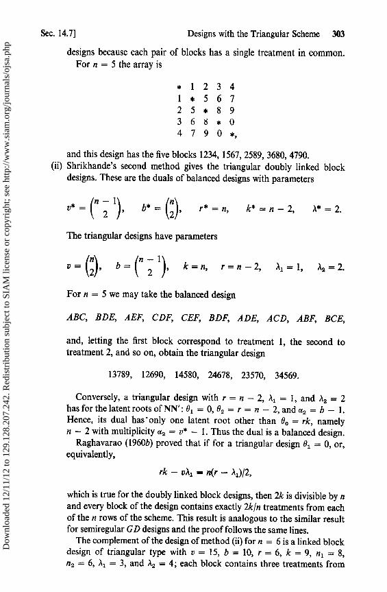
Sec. 14.7]
Designs with the Triangular Scheme 303
designs because each pair of blocks has a single treatment in common.For n = 5 the array is
* 1 2 3 41 * 5 6 72 5 * 8 93 6 8 * 04 7 9 0 *,
and this design has the five blocks 1234, 1567, 2589, 3680, 4790.(ii) Shrikhande's second method gives the triangular doubly linked block
designs. These are the duals of balanced designs with parameters
v (fl
;= 1) b* = (n)
* 2,r* = n, k*=n -2, ,1*=2.
The triangular designs have parameters
v =(n) b=(n 2 1), k=n, r=n -2, Al =1, )L2 =2.
For n = 5 we may take the balanced design
ABC, BDE, AEF, CDF, CEF, BDF, ADE, ACD, ABF, BCE,
and, letting the first block correspond to treatment 1, the second totreatment 2, and so on, obtain the triangular design
13789, 12690, 14580, 24678, 23570, 34569.
Conversely, a triangular design with r = n — 2, Al = 1, and '2 = 2has for the latent roots of NN' : 8 1 = 0, 02 = r = n — 2, and a2 = b — 1.Hence, its dual has' only one latent root other than Bo = rk, namelyn — 2 with multiplicity a2 = v* — 1. Thus the dual is a balanced design.
Raghavarao (1960b) proved that if for a triangular design Bl = 0, or,equivalently,
rk — vAl = n(r — Al)12,
which is true for the doubly linked block designs, then 2k is divisible by nand every block of the design contains exactly 2k/n treatments from eachof the n rows of the scheme. This result is analogous to the similar resultfor semiregular GD designs and the proof follows the same lines.
The complement of the design of method (ii) for n = 6 is a linked blockdesign of triangular type with v = 15, b = 10, r = 6, k = 9, n l = 8,n2 = 6, A l = 3, and '2 = 4; each block contains three treatments from
Dow
nloa
ded
12/1
1/12
to 1
29.1
28.2
07.2
42. R
edis
trib
utio
n su
bjec
t to
SIA
M li
cens
e or
cop
yrig
ht; s
ee h
ttp://
ww
w.s
iam
.org
/jour
nals
/ojs
a.ph
p

304 The Existence and Construction of Partially Balanced Designs [Ch. 14
each row of the scheme. It is the dual of the balanced design withparameters
v* = 10, b* = 15, r * = 9 = n(n - 3)/2,
k* = 6 = (n - 2)(n - 3)/2, A* = 5 = (n - 1)(n - 4)/2.
It follows from the foregoing discussion that all triangular designs withr = n - 2, A l = 1, and X12 = 2 are doubly linked block designs and thatthe existence of such a design for any n implies the existence of thecorresponding balanced design. For n = 7, 8, 10 the correspondingdesigns would be balanced designs with parameters
v= 15,k=5,A=2; v=21,k=6,A=2; v=36,k=8,A=2.
However, Hall and Connor (1953) showed that these three designs areimpossible. This implies that triangular designs with r = n - 2, A l = 1,and a2 = 2 do not exist for n = 7, 8, or 10.
(iii) Each of the rows in the scheme constitutes a set of (n - 1) varieties withthe property that any pair of theet are first associates. If there exists abalanced incomplete block design with parameters v* = n - 1, b*, r*,k* = k, A*, we can take such a design for each row of the scheme andcombine theet into a triangular design with
v = n(n - 1)/2, b = nb*, r = 2r*, k, A = \*, ,1 2 = 0.
For n = 5, v = 10, and k = 3, we note that each row of the schemehas n - 1 = 4 varieties and use the balanced design with v = b = 4,r = k = 3 to obtain the design
123, 156, 258, 368, 479,124, 157, 259, 360, 470,134, 167, 289, 380, 490,234, 567, 589, 680, 790.
For k >- 4, this is the only way of obtaining a design with A, = 0.Hence, a triangular design with 4 < k < n - 1, r, )t, and AZ = 0 existsif, and only if, a balanced incomplete block design with v* = n - 1,k* = k >_ 4, r* = r/2, and A* = Al exists.
(iv) The method of triads is due to Clatworthy. When k = 3, method (iii)is not the only method of obtaining a design with A > 0 and A2 = 0.Another method is to obtain the blocks as follows. Take a pair ofvarieties that appear in the same row. The first variety appears again inanother row. For the third member of the block take the variety that
Dow
nloa
ded
12/1
1/12
to 1
29.1
28.2
07.2
42. R
edis
trib
utio
n su
bjec
t to
SIA
M li
cens
e or
cop
yrig
ht; s
ee h
ttp://
ww
w.s
iam
.org
/jour
nals
/ojs
a.ph
p

Sec. 14.9] Designs for the Latin Square Scheme 305
appears in that row and in the same column as the second member. Thus,in the case n = 5 the blocks would be
125, 136, 147, 238, 249,
340, 568, 579, 670, 890.
In the general case, r = n - 2, 6b = n(n - 1)(n - 2).
14.8 The Nonexistence of Some Triangular Designs
The latent roots of NN' are not negative; thus it is necessary that
r +(n- 4);11 -(n- 3)12 >0, r-211 +A2 >_0.
This rules out, for example, designs with parameters
n = 5, v = 10, r = 9, k = 5, b = 18,1 1 = 2,A2 =8,(61 =- 5);
n=5,v= 10,r=3,k=5,b=6, A 1 =2,12 =0,(02 =- 1).
For symmetric designs it is necessary that
I NNI = r20n-102(n-3)12
be a square. If neither 0 nor 0 2 is zero, it follows that
(i) If n = 4t, 0 must be a square;(ii) If n = 4t + 1, 02 must be a square;(iii) If n = 4t +2, 01 02 must be a square.
Examples of designs that are found to be nonexistent by these criteria are
(a) n = 8,v = b = 28,r = k = 10, d1 =5,A2 =2,(0 = 20);(b)n= 9,v=b=36,r=k=8, A1 = 1,12 =2,(82 =8);(c) n= 6,v=b= 15,r=k=5, A 1 = 1,,12 =2,(91 62 =5).
Further such conditions involving the Hasse-Minkowski invariant are givenby Ogawa (1959).
14.9 Designs for the Latin Square Scheme
These designs are discussed by Clatworthy (1956) and (1967), and by Changand Liu (1964). They include as a special case the designs obtained by takingsome, but not all, of the replicates in the Yates orthogonal series designs for
Dow
nloa
ded
12/1
1/12
to 1
29.1
28.2
07.2
42. R
edis
trib
utio
n su
bjec
t to
SIA
M li
cens
e or
cop
yrig
ht; s
ee h
ttp://
ww
w.s
iam
.org
/jour
nals
/ojs
a.ph
p

306 The Existence and Construction of Partially Balanced Designs [Ch. 14
v = k2, b = k(k + 1), r = k + 1, and \ = 1. Clatworthy (1956) gives a listingof 111 designs most of which are L 2 designs. Chang and Liu have calculated thatthere are 155 combinations of parameters that might lead to L2 designs withr < 10 and k <_ 10. Of these, seventy-two are included in Clatworthy's listing;Chang and Liu give twenty-one others and show that fifty-seven of the designsdo not exist. The five unsolved cases are
v=36, k=6, r=9, X11 =2, A2 =1,v=36, k=6, r=10, a1 =0, ,^2 =2,v=36, k=9, r=10, ,i1 =3, A2 =2,v=49, k=9, r=9, A=3, A2 =1,v = 100, k = 10, r = 9, a1 =0, ,12 =1.
Shrikhande (1959b) has shown that the L2 scheme is unique except for n = 4.In this case there are two schemes with v = 16, n, = 6, n 2 = 9, and pi l = 2.The second scheme arises when, in one of the L 3 schemes, we interchange firstand second associates. Suppose that the square array and the Latin square are
1 2 3 4 ABCD5 6 7 8 BCDA9101112 CDAB
13141516 DABC.
Let two varieties be first associates if they do not appear in the same row orcolumn or with the same letter; this gives a set of parameters v = 16, n l = 6,n2 = 9, and pi l = 2 as in the L2 scheme, but consider the first associates ofvariety 1. They are 6, 7, 10, 12, 15, and 16. The first associates of 6 are 1, 4, 11, 12,13, and 15, and so varieties 12 and 15 are first associates of both 1 and 6. If thescheme is an L2 scheme, it follows that 1, 6, 12, and 15 must appear in the samecolumn or row of a square array and, hence, 12 and 15 are first associates.Twelve and 15 both go with the letter B, and so they are second associates, incontradiction. This scheme was first mentioned by Mesner (1956) and (1967).
In the same paper Shrikhande gives conditions for the nonexistence of sym-metric L2 designs based on the Hasse-Minkowski invariant.
The latent roots of NN' and their multiplicities are
01 =r-(i-n)(Al -,la)-,12, a1 =i(n- 1),
02=r - i(Al - A2) - '12, a2=(n-1)(n-i+ 1).
For the La case, a l is always even; a2 is odd when n is odd, and then 02 = r -2a1 + a2 must be a square if the design is symmetric and B l > 0.
Raghavarao (1960b) gives a result for L 2 designs similar to those justmentioned for semiregular GD designs and triangular designs. If rk - v211 =n(r - A'), then k is divisible by n and every block of the design contains kinvarieties from each row of the association scheme. It should be noted, however,that this condition is not equivalent either to 0 = 0 or to 02 = 0.
Dow
nloa
ded
12/1
1/12
to 1
29.1
28.2
07.2
42. R
edis
trib
utio
n su
bjec
t to
SIA
M li
cens
e or
cop
yrig
ht; s
ee h
ttp://
ww
w.s
iam
.org
/jour
nals
/ojs
a.ph
p

Sec. 14.9] Designs for the Latin Square Scheme 307
Clatworthy (1967) has shown that most of the known L, designs belong tofour families. We shall discuss each of the families in turn. Our notation differsfrom that of Clatworthy in that he talks of v = s 2 varieties while we havev = n2 . We shall alter the definitions of families A and D slightly in order toinclude more designs. Clatworthy considers numerous special cases in eachfamily; the reader is referred to his paper for these.
Family A: These are designs with k < n and a2 = 0. Let D be a balancedincomplete block design with parameters v* = n, b*, k* = k, r*, d* = A l . Thefirst b* blocks of our design consist of the blocks of D using the varieties in thefirst row of the square array of the association scheme; D is then repeated usingthe varieties in the second row, and so on. After all the rows have been used, werepeat the procedure using the columns of varieties. If i > 2, the procedure isthen repeated again for each of the i — 2 orthogonal squares. We then have adesign with
b = inb*, r = ir*, k, i\, A2 = 0.
If the balanced design D is the unreduced design consisting of all (k) subsets of
k out of the n varieties, we have
n-2b=ni(n)
k' Al=(k-2)' A2=0.
If k = n, the design consists of ni blocks forming the first i replicates of thebalanced lattice, if that design exists, with A l = 1 and A2 = 0. We shall use thisdesign later.
Family B: These are designs with k = 2n. The first n(n — 1)/2 blocks consist ofall possible pairs of rows from the square array, the next n(n — 1)/2 blocksconsist of pairs of columns, and so on. For the L i design we have
b=in(n — 1)/2,r=i(n— 1),k=2n, l =n+i-2,A2 =i.
Family C. These designs have k = n, and they exist whenever n is a prime, or apower of a prime. We have already mentioned the design in family A withk = n, Al = 1, and A2 = 0. If we proceed in the same way to set up a seconddesign using the remaining Latin squares of the complete orthogonal set, weshall have a second design with b = n(n — i + 1), k = n, A l = 0, and A 2 = 1.If we wish to construct a design with parameters al , Â, we have now merely torepeat the first design d l times and the second design X2 times. The reader wiltappreciate that if there exists a balanced design with A = 1 for a value of k <_ s,we may use a similar. procedure.
Dow
nloa
ded
12/1
1/12
to 1
29.1
28.2
07.2
42. R
edis
trib
utio
n su
bjec
t to
SIA
M li
cens
e or
cop
yrig
ht; s
ee h
ttp://
ww
w.s
iam
.org
/jour
nals
/ojs
a.ph
p

308 The Existence and Construction of Partially Balanced Designs [Ch. 14
Family D: This family consists of the ES(i) and E'S(i) designs. The parametersfor these symmetric designs are
ES(1): k = i(n — 1), ,1 1 =i 2 -3i+n, d2 =i(i— 1),ES(2): k=(n-1)(n—i+ l), ) 1 =(n—i)(n—i+ l),
X12 =(n—i)2 +i-2,E'S(l): k=i(n-1)+1, a1 =i 2 -3i+n+2, A2 =i(i— 1),E'S(2): k=(n-1)(n—i+1)+1, A1 =(n—i)(n—i+1),
A2 =(n—i) 2 +i.
Exercises
1. Prove that if A and B are square matrices such that AB and BA both exist, thenAB and BA both have the same nonzero latent roots.
2. Derive the P matrices for Shrikhande's two linked block designs.3. Let U be a square matrix of order mn partitioned into m 2 square matrices U, of
order n where U 5 = al,, + bJn if i = j, and cIn + dJn if i ^ j. Recalling thatlaI. + bJnl = an-1 (a + nb), show that
U = (a — C)(n-1)(m-1)(a + nb — c — nd)m - '(a + (m — 1)c)n - 1
x {a + nb + (m — 1)(c + nd)}.
4. (Continuation). Order the varieties of a GD scheme so that the ith groupconsists of varieties (i — 1)n + 1, ..., in. Then evaluate directly the determinantINNI•
5. (Continuation). Show that if the varieties in an L2 scheme are suitably ordered
INN'I = rk(r + (n — 2),11 — (n — 1)) 2)2(n -1)(r — 2A1 + ,12)(n -1)2 .
Hence find the latent roots of NN' and their multiplicities.6. Prove that if a triangular design has 0 1 = 0 then 2k is divisible by n and each
block contains exactly 2k/n treatments from each row of the scheme [Raghavarao(1960b)].
7. Prove that if, in a design with the L2 scheme,
rk—val =n(r— ,11),
then k is divisible by n and every block of the design contains kin treatmentsfrom each row of the scheme [Raghavarao (1960b)].
8. Show that for any L 2 design the following inequalities hold for b. Leta = min(n — 1, [r/Â1 ]), p = min(n — 1, [r/,12]), where [x] is the integer part of x.Then [Chang and Liu (1964)]
2b >— (a + 1)(2r — aal), 2b >— (P + 1)(2r —
Dow
nloa
ded
12/1
1/12
to 1
29.1
28.2
07.2
42. R
edis
trib
utio
n su
bjec
t to
SIA
M li
cens
e or
cop
yrig
ht; s
ee h
ttp://
ww
w.s
iam
.org
/jour
nals
/ojs
a.ph
p

Exercises 309
9. Consider a PBIB(2) association scheme A in which there exists a set of u,treatments that are all i th associates of each other. Let
wt = min(u i — 1, [r/,1,]), wi = min(u1 — 1, [(b — r)/(b — 2r + a{)]).
Show that for any design having associate scheme A
2b >— (w { + 1)(2r — w) i), 2b > (wi + 1)(2b — 2r — wí(b — 2r + ai)).
Adapt this result to obtain a nonexistence theorem for triangular designs[Chang, et al. (1965)].
10. Show that for any PBIB(2) design which is not of the GD type [Chang et al.(1965)],
max(2,1, — A2, 2) 2 — Al) < r.
Dow
nloa
ded
12/1
1/12
to 1
29.1
28.2
07.2
42. R
edis
trib
utio
n su
bjec
t to
SIA
M li
cens
e or
cop
yrig
ht; s
ee h
ttp://
ww
w.s
iam
.org
/jour
nals
/ojs
a.ph
p
CHAPTER 15
AdditionalTopics in
Partially BalancedDesigns
In this chapter we shall continue our investigation of partially balanceddesigns, with emphasis on designs having more than two associate classes. Webegin, however, with a short introduction to the topic of partial geometries andtheir application to PBIB (2) designs.
We have already emphasized the usefulness of the latent roots of NN' indetermining the nonexistence of some designs. We shall discuss the subject of thelatent roots of NN' and their multiplicities in PBIB(m) schemes at some length.The discussion of that topic will conclude with a few words about cyclic andpseudocyclic schemes with two associate classes. In the succeeding section, weshall introduce several PBIB(3) schemes. The chapter will conclude with adiscussion of cyclic designs.
15.1 Geometric Designs
In the previous chapter we dealt with designs having the three principal typesof schemes with two associate classes: group divisible, triangular, and Latinsquare. There was only one reference to designs obtained from finite geometries,and that example duplicated a design given earlier. Finite geometries do, how-ever, provide a series of simple partially balanced designs, i.e., designs havingeither Al = 1, .2 = 0, or Al = 0, A2 = 1, which do not belong to the threeprincipal types.
Bose and Nair (1939) presented several examples of designs obtained fromEuclidean or projective geometries. If we consider the set of all lines in aEuclidean geometry with sN points and omit all the lines that pass through theorigin 0, we can let points denote varieties and lines denote blocks. The remaining
310
Dow
nloa
ded
12/1
1/12
to 1
29.1
28.2
07.2
42. R
edis
trib
utio
n su
bjec
t to
SIA
M li
cens
e or
cop
yrig
ht; s
ee h
ttp://
ww
w.s
iam
.org
/jour
nals
/ojs
a.ph
p

Sec. 15.1] Geometric Designs 311
points and lines form a GD design for v = sN — 1 varieties in blocks of sizek = s with A l = 0 and A2 = 1. Two varieties are first associates if the linejoining the points passes through the origin. Then n l = s — 1.
Other GD designs are obtained if we consider m-dimensional subspaces(m > 1) and again omit those subspaces that contain the origin O. Bose andNair also considered omitting from a projective geometry, PG(2, s = p"), all thepoints on three lines that are not concurrent, and all the lines passing through thevertices of the triangle formed by those three lines.That procedure led them tosome symmetric L 3 designs with v = (s — 1) 2, k = (s — 2), X12 = 1, and A l = 0.
More interesting, perhaps, are the designs obtained from partial geometriesbecause every partial geometry is isomorphic to a simple PBIB(2) design. Apartial geometry is a collection of v points (varieties) and b lines (blocks) withthe following axioms:
(i) There is only one line through any pair of points;(ii) There are exactly k points on each line;(iii) There are exactly r lines through each point;(iv) If a point P does not lie on a line p, then there are exactly t lines through P
that intersect p.
This system constitutes a partial geometry with parameters (r, k, t). It followsthat
tv=k[(r— 1)(k— 1) + t],tb = r[(r— 1)(k— 1) + t].
To derive the latter relationship, we note that there are r lines passing throughP, each with k — 1 points other than P. Thus, there are r(k — 1) points con-nected to P. On the other hand, there are b — r lines that do not pass through P.Each of these b — r lines contains t points that are connected to P; each of thepoints is on r — 1 of the b — r lines; thus, there are t(b — r)/(r — 1) pointsconnected to P. Hence,
r(k — 1) = t(b — r)/(r — 1) and b = r[(r — 1)(k — 1) + t]/t.
If we now let points denote varieties and lines denote blocks, we have a simplepartially balanced design. Two varieties are first associates if their points areconnected in the partial geometry; otherwise, they are second associates. Wehave nl = r(k — 1), n 2 = (r — 1)(k — 1)(k — t)/t. To obtain pi l we considertwo first associates P and Q. There are k — 2 other points on PQ. There arer — 1 lines through Q other than PQ; each of these lines contains t first associatesof P. Thus,
P1,=(t-1)(r-1)+k-2, P12 = (r— 1)(k — t),
Pij=rt, P12= r(k —t-1).
Dow
nloa
ded
12/1
1/12
to 1
29.1
28.2
07.2
42. R
edis
trib
utio
n su
bjec
t to
SIA
M li
cens
e or
cop
yrig
ht; s
ee h
ttp://
ww
w.s
iam
.org
/jour
nals
/ojs
a.ph
p

312 Additional Topics in Partially Balanced Designs [Ch. 15
Bose and Clatworthy (1955) show that every PBIB(2) design with A l = 1,sla = 0, and b < v is a partial geometry. It follows that the singly linked blockdesigns are partial geometries. These are one of the series of linked blockdesigns obtained by Shrikhande (1952), and are duals of the balanced incom-plete block designs with v* = rk — k + 1, r* = k, k* = r, and A* = 1. Theywere mentioned at the beginning of Chapter 14. When r = 2, the singly linkedblock design is a triangular design. Thus the triangular association scheme canbe obtained from a partial geometry configuration.
For a further discussion of this topic the reader is referred to the review paperby Bose (1963) and the two monographs by Vajda (1967a,b). Further research inthis area is being carried out by students of graph theory. The representation ofassociation schemes as concordant graphs is mentioned by Bose and Mesner(1959).
Mesner (1967) has extended the Li scheme to include cases where n and i areboth negative, although all the design parameters are positive. This gives the NLfamily of schemes (negative Latin square). The NL(n) scheme has v = n2 , andthe other parameters are obtained by putting —n for n and —i for i in thecorresponding formulae for the L i scheme. For example, the NL3(8) scheme hasv=64, n 1 =-3(-8-1)=27, n 2 =(-8+3+1)(-8-1)=36. The Pmatrices are
P1 = [16 20,' P2 = [15 20]
Numerous designs with NL schemes can be obtained from finite geometries,and Mesner gives some examples in the reference cited.
15.2 Latent Roots of the Intrablock and Interblock Matrices
The formula for the intrablock efficiency of an incomplete block designobtained at the end of Chapter 11 involves the nonzero latent roots of A. Wehave seen that for a linked block design A has a single nonzero latent root withmultiplicity b — 1. We now investigate further the latent roots of A and NN' forPBIB designs.
In solving the intrablock equations for the case of two associate classes(Chapter 12) we obtained (12.2). Adding the quantity Ji= 1 )iln lfi gives
kSl(Qh) = Sl(Th){r(k — 1) — A1Pii — A2Pi2 + it lnl}+S2(^h){ — a1P1 — '2Pi2 + Alnl}.
In the general case of m associate classes
Si(Qh) = i 9'iƒSJ(fh),j=1
where kpi! = r(k — 1 )Si, — ^k=1 AkPik + Aini, and Bij is the Kronecker delta.
Dow
nloa
ded
12/1
1/12
to 1
29.1
28.2
07.2
42. R
edis
trib
utio
n su
bjec
t to
SIA
M li
cens
e or
cop
yrig
ht; s
ee h
ttp://
ww
w.s
iam
.org
/jour
nals
/ojs
a.ph
p
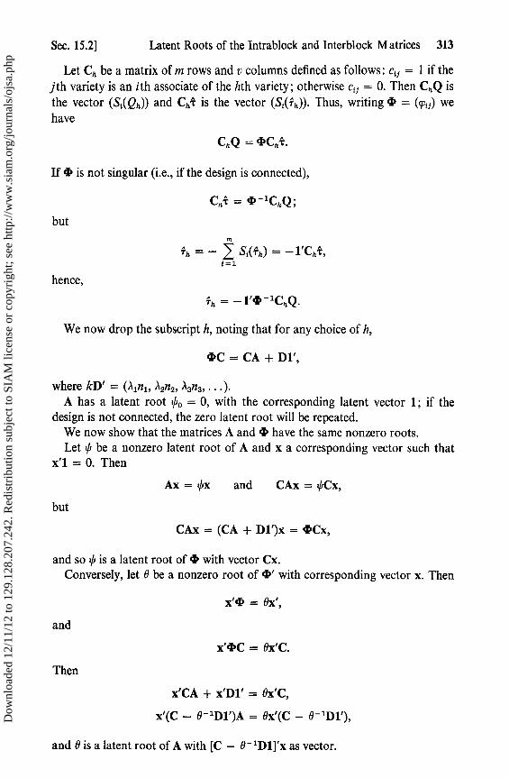
Sec. 15.2] Latent Roots of the Intrablock and Interblock Matrices 313
Let Ch be a matrix of m rows and v columns defined as follows: c i; = 1 if thejth variety is an ith associate of the hth variety; otherwise cl; = 0. Then ChQ isthe vector (Si(Qh)) and Ch-r is the vector (Si(fh)). Thus, writing < _ (W) wehave
C,Q = 4'C, zT.
If <b is not singular (i.e., if the design is connected),
C,T ='D -1C,Qi
but
Th = - Si(Th) _ -1 ' ChT,t=1
hence,
fh = — 1'b - 1 ChQ•
We now drop the subscript h, noting that for any choice of h,
^C = CA + Dl',
where kD' = (A 1n1 , A2n2 , i\an3 , ... ).
A has a latent root 0 o = 0, with the corresponding latent vector 1; if thedesign is not connected, the zero latent root will be repeated.
We now show that the matrices A and 4 have the same nonzero roots.Let 0 be a nonzero latent root of A and x a corresponding vector such that
x'1 = 0. Then
Ax = Ox and CAx = OCx,
but
CAx = (CA + D1')x = ^Cx,
and so 0 is a latent root of <D with vector Cx.Conversely, let 0 be a nonzero root of ' with corresponding vector x. Then
x' I = Ox',
x'^C = Ox'C.
x'CA + x'Dl' = Ox'C,
x'(C — 0 'Dl')A = Ox'(C — 0 -1D1'),
and 0 is a latent root of A with [C — 0 - 'D1]'x as vector.
and
Then
Dow
nloa
ded
12/1
1/12
to 1
29.1
28.2
07.2
42. R
edis
trib
utio
n su
bjec
t to
SIA
M li
cens
e or
cop
yrig
ht; s
ee h
ttp://
ww
w.s
iam
.org
/jour
nals
/ojs
a.ph
p

314 Additional Topics in Partially Balanced Designs [Ch. 15
Let II* = (p 1) wherem
= r8i1 + 1 AkPtik — niAi,k=1
thenk> = krI — II*.
Since kA = rkI — NN', it follows that if B i is a latent root of NN' withmultiplicity a, then 0i = (rk — 8)/k is a root of A with the same multiplicity a,.It also follows, from the similar relationship between 4; and II*, that because thenonzero roots of c are the nonzero roots of A, the roots of NN' are, with theexception of rk, the same as the roots of II*. This result was first shown byConnor and Clatworthy (1954). Bose and Mesner (1959) derived it by consideringthe algebra of the association matrices; in their paper they also proved that themultiplicities a i are independent of r, Al, A2, ..., Am. Since NN' is nonnegativedefinite, none of its roots are negative.
The ith association matrix Bi is defined as follows: the element Pab in the athrow and bth column, 0 <_ a <_ m, 0 5 b <_ m, is 1 if a and b are ith associatesand zero otherwise.
The equation 1 1I* = 0 is a polynomial of the mth degree in r. If the deter-minant vanishes when r takes the values s 1 , s2i . .., sm , the corresponding latentroots of fl*, and hence of NN', are B, = r — si . The zeros s,, are linear functionsof the Ai, and so we may write
9=rl+Z*?,
where 0' = (0k, 02, ... , Om), X' _ (A1, A2, ... , am).Adding the root 0 = rk, we have
tr (NN') = rv = rk +s=1
or, writing a' = (al, «2, ... , am), n ' = (n1, %12, ... , nm),
r(v—k)=a'@=ra'l+a'Z*1^.
Then, since á 1 = v — 1,
a'Z*a=—r(k-1)=—n'X,
which is, since the a i are independent of the ,\, an identity in the A t . This leads tom equations to be solved for the m unknowns al , ..., am , (Z*)'a = —n.
For two associate classes det 11* = 0 is a quadratic in 0. Connor and Clat-worthy (1954) have shown that after some simplification it may be written
(r — 0)2 + KAl — "2)(Pi2 — P112) — (Al + A2)](r — 0)
+ [(A1 — '2)(Q2P112 — A1P212) + A1A2] = 0,
Dow
nloa
ded
12/1
1/12
to 1
29.1
28.2
07.2
42. R
edis
trib
utio
n su
bjec
t to
SIA
M li
cens
e or
cop
yrig
ht; s
ee h
ttp://
ww
w.s
iam
.org
/jour
nals
/ojs
a.ph
p

Sec. 15.3] Cyclic Association Schemes 315
whence, putting y = Pi2 — Pi2, = P12 + P12, and 0 = y2 + 2P + 1, itfollows that
01= r++(/D+Y — 1 )Al — f(1/O+y+ 1)A2,
92= r — j(4/ 1 —y+ 1 ) )ti+ (1/0— y — 1)a2 .
Furthermore,
nl + n2 (nl — n2) + Y(n1 + n2)a= 2 — 2/
and
nl + n2 (n l — n2) + y(nl + n2)
a= 2 +2\/Q
It is necessary that these multiplicities be positive integers. This imposes somerestrictions upon the parameters for the existence of designs, especially if A isnot a perfect square.
We calculate now the latent roots and their multiplicities for a group divisibledesign. In this case
IH*I = Ir —Al (A2 — — 1)0 r + Ál(n — 1) — ÁZn2
1
whence 0 1 =r+) 1(n-1)—,12n=rk—vA2 and 02 =r —X1 1 . We havey= P= n-1andA= n2 .Hence,
a 1 =m-1, a2 =m(n-1).
Bose and Connor (1952) obtained this result directly by evaluating NN'I _rk(rk — v12)m -1 (r — ,\ )m(n -1 ). Alternatively,
Z* — n-1 n (Z*)_1 = — i 0 n
0] n [1 n — 1]
_ _ n (Z*)-i = n [(n — 1), n(m — 1)] L? n 1J
= [(m — 1), m(n — 1)].
15.3 Cyclic Association Schemes
We have already noted that the requirements that the latent roots Bt be non-negative and that for a symmetric design the determinant NN'1 be a squareenable us to establish that designs with certain sets of parameters do not exist.In all the standard association schemes for PBIB(m) designs, the formulae for a,automatically give only integer values, and so the requirement that a, be aninteger is not very helpful. It is of interest, however, in the schemes for twoassociate classes when we consider the results of Connor and Clatworthy thathave just been obtained. If 0 is not a square, VA is irrational and the term
Dow
nloa
ded
12/1
1/12
to 1
29.1
28.2
07.2
42. R
edis
trib
utio
n su
bjec
t to
SIA
M li
cens
e or
cop
yrig
ht; s
ee h
ttp://
ww
w.s
iam
.org
/jour
nals
/ojs
a.ph
p
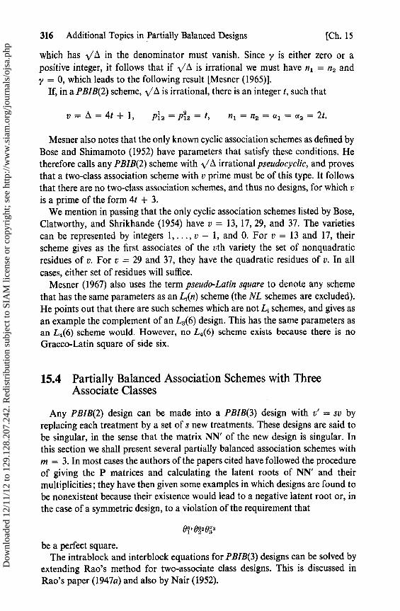
316 Additional Topics in Partially Balanced Designs [Ch. 15
which has -,/A in the denominator must vanish. Since y is either zero or apositive integer, it follows that if -/A is irrational we must have n l = n2 andy = 0, which leads to the following result [Mesner (1965)].
If, in a PBIB(2) scheme, -/A is irrational, there is an integer t, such that
v=11 =4t+1, p12=pi2=t, n 1 =n2 =«2 = a2 =2t.
Mesner also notes that the only known cyclic association schemes as defined byBose and Shimamoto (1952) have parameters that satisfy these conditions. Hetherefore calls any PBIB(2) scheme with %/0 irrational pseudocyclic, and proventhat a two-class association scheme with v prime must be of this type. It followsthat there are no two-class association schemes, and thus no designs, for which vis a prime of the form 4t + 3.
We mention in passing that the only cyclic association schemes listed by Bose,Clatworthy, and Shrikhande (1954) have v = 13, 17, 29, and 37. The varietiescan be represented by integers 1, ..., v — 1, and 0. For v = 13 and 17, theirscheme gives as the first associates of the vth variety the set of nonquadraticresidues of v. For v = 29 and 37, they have the quadratic residues of v. In allcases, either set of residues will suffice.
Mesner (1967) also uses the term pseudo-Latin square to denote any schemethat has the same parameters as an L(n) scheme (the NL schemes are excluded).He points out that there are such schemes which are not L, schemes, and gives asan example the complement of an L3(6) design. This has the same parameters asan L4(6) scheme would. However, no L4(6) scheme exists because there is noGraeco-Latin square of side six.
15.4 Partially Balanced Association Schemes with ThreeAssociate Classes
Any PBIB(2) design can be made into a PBIB(3) design with v' = sv byreplacing each treatment by a set of s new treatments. These designs are said tobe singular, in the sense that the matrix NN' of the new design is singular. Inthis section we shall present several partially balanced association schemes withm = 3. In most cases the authors of the papers cited have followed the procedureof giving the P matrices and calculating the latent roots of NN' and theirmultiplicities; they have then given some examples in which designs are found tobe nonexistent because their existence would lead to a negative latent root or, inthe case of a symmetric design, to a violation of the requirement that
Bil B2O3
be a perfect square.The intrablock and interblock equations for PBIB(3) designs can be solved by
extending Rao's method for two-associate clans designs. This is discussed inRao's paper (1947a) and also by Nair (1952).
Dow
nloa
ded
12/1
1/12
to 1
29.1
28.2
07.2
42. R
edis
trib
utio
n su
bjec
t to
SIA
M li
cens
e or
cop
yrig
ht; s
ee h
ttp://
ww
w.s
iam
.org
/jour
nals
/ojs
a.ph
p
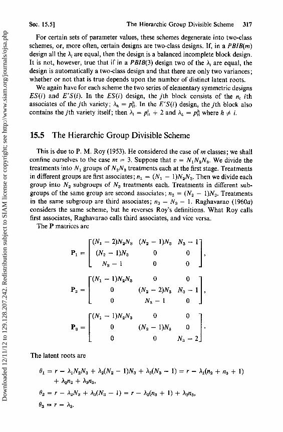
Sec. 15.5] The Hierarchic Group Divisible Scheme 317
For certain sets of parameter values, these schemes degenerate into two-classschemes, or, more often, certain designs are two-class designs. If, in a PBIB(m)design all the A, are equal, then the design is a balanced incomplete block design.It is not, however, true that if in a PBIB(3) design two of the A, are equal, thedesign is automatically a two-class design and that there are only two variances;whether or not that is true depends upon the number of distinct latent roots.
We again have for each scheme the two series of elementary symmetric designsES(i) and E'S(i). In the ES(i) design, the jth block consists of the n i ithassociates of the jth variety; dh = p. In the E'S(i) design, the jth block alsocontains the jth variety itself; then d t = p; ; + 2 and ,, = p 1 where h i.
15.5 The Hierarchic Group Divisible Scheme
This is due to P. M. Roy (1953). He considered the case of m classes; we shallconfine ourselves to the case m = 3. Suppose that v = N1N2N3 . We divide thetreatments into Nl groups of N2N3 treatments each at the first stage. Treatmentsin different groups are first associates; n l = (Nl — 1)N2N3 . Then we divide eachgroup into N2 subgroups of N3 treatments each. Treatments in different sub-groups of the same group are second associates; n2 = (N2 — 1)N3 . Treatmentsin the same subgroup are third associates; n3 = N3 — 1. Raghavarao (1960a)considers the same scheme, but he reverses Roy's definitions. What Roy callsfirst associates, Raghavarao calls third associates, and vice versa.
The P matrices are
(Ni — 2)N2N3 (N2 — 1)N3 N3 — 1
P1 = (N2 — 1)N3 0 0
N3 -1 0 0
(Ni — 1)N2N30 0
P2 = 0 (N2 — 2)N3 N3 — 1
0 N3-1 0
(Ni — 1)N2N30 0
P3 = 0 (N2-1)N3 0
0 0 N3-2
The latent roots are
B1= r — A1N2N3+\2(N2 -1 )N3+A3(N3 - 1)=r—Al(n2+n3+1)
+ X2n2 + A3n3,
03= r — A2N3+A3(N3 -1)=r — i2(n3+ 1 )+ )an3,
03= r —.13.
Dow
nloa
ded
12/1
1/12
to 1
29.1
28.2
07.2
42. R
edis
trib
utio
n su
bjec
t to
SIA
M li
cens
e or
cop
yrig
ht; s
ee h
ttp://
ww
w.s
iam
.org
/jour
nals
/ojs
a.ph
p

318 Additional Topics in Partially Balanced Designs [Ch. 15
To find the multiplicities we solve
— (n2 + n3 + 1) 0 0 [al] nl
n2 —(n3 + 1) 0 a2 = — n2
n3 n3— 1 a3 n3
and obtain
al = Nl — 1, a2 = N1(N2 — 1), a3 = N1N2(N3 — 1).
Roy (1953) gives the following example of a resolvable design with parameters
v =8, b=10, r=5, k=4, N 1 =N2 =N3 =2,
n1=4, n2=2, n3 =1, A1 =2, A2 =3, ,13 =1:
1234, 5678; 1357, 2468; 1368, 2457; 1458, 2367; 1467, 2358.The subgroups are 12, 34; 56, 78.
If A2 = a3 , the design is merely a GD design with Nl groups, each of which hasN2N3 treatments. In this case, 92 = 03 = r — A3 , and there are only two distintroots.
15.6 The Rectangular Scheme
Vartak (1959) discusces designs with this scheme and calls them series A.Suppose that we arrange v = mn treatments in a rectangular array of m rowsand n columns. Treatments are first associates if they appear in the same row,and second associates if they appear in the same column; otherwise they arethird associates. Then n l = n — 1, n 2 = m — 1, and n3 = (m — 1)(n — 1),
n-2 0 0
P1 = 0 0 m-1
0 m-1 (m-1)(n-2)
0 0 n-1
P2 0 m-2 0
n-1 0 (m-2)(n-1)
0 1 n-2
P3 = 1 0 m-2
n-2 m-2 (m-2)(n-2)
Dow
nloa
ded
12/1
1/12
to 1
29.1
28.2
07.2
42. R
edis
trib
utio
n su
bjec
t to
SIA
M li
cens
e or
cop
yrig
ht; s
ee h
ttp://
ww
w.s
iam
.org
/jour
nals
/ojs
a.ph
p

Sec. 15.7]
The Cubic Scheme 319
0 1 =r—A l +(m-1)(%2--fis), a1= n-1=n1,
02 =r +(n-1)(,11 —a3)- 2 , «2= m-1 =n2,
B3 =r—A1 — X12 +,13 , «3= (m-1)(n-1) =n3.
Vartak also proves that the scheme is unique in the sense that if a PBIB(3)association scheme has P matrices identical with those above, then the schememust be a rectangular scheme.
If m = n and also X1 1 = we have designs with the L2 scheme. In this caseBl = 02 . Note, however, that unless the array is square, putting A l = ,12 will notmake the two roots equal, and the number of associate classes is still three.
15.7 The Cubic Scheme
This is due to Raghavarao and Chandrasekhararao (1964). There arev = s3 treatments, each of which is denoted by a different set of three co-ordinates (x, y, z) where x, y, and z are all integers such that 1 < x < s,1 < y < s, 1 < z < s. Two treatments are defined to be i th associates if theyhave exactly (3 — i) coordinates in common. For convenience we write (x, y, z)as xyz. Thus, for s = 3, v = 27, the treatment 000 has six first associates:001, 002, 010, 020, 100, and 200. It has eight third associates denoted by abc,where each of the coordinates a, b, and c takes the values 1 or 2. In the generalcase, nl = 3(s — 1), n2 = 3(s — 1)2, and n3 = (s — 1)3 .
s-2 2(s-1) 0
Pl = 2(s — 1) 2(s — 1)(s — 2) (s — 1)2
,
0 (s — 1)2 (s — 1)2(5 — 2)
2 2(s-2) (s— 1)
P2 = 2(s — 2) 2(s — 1) + (s — 2)2 2(s — 1)(s — 2)
(s — 1) 2(s — 1)(s — 2) (s — 1)(s — 2) 2
0 3 3(s-2)
P3 = 3 6(s — 2) 3(s — 2)2
3(s — 2) 3(s — 2)2 (s — 2)3
The latent roots of NN' and their multiplicities are
Bo =rk, 01 =r+(2s-3))) 1 +(s-1)(s-3)) 2 — (s- 1)2A3 ,
02 =r+(s- 3)Al —(2s-3)A2 +(s— 1) 3i 03 = r-3A1 +3A2 —Al ,
ao =1, a1 =3(s-1) =n1, a2 =3(s-1)2 =n2, a3= (s- 1)3 =n3.
Dow
nloa
ded
12/1
1/12
to 1
29.1
28.2
07.2
42. R
edis
trib
utio
n su
bjec
t to
SIA
M li
cens
e or
cop
yrig
ht; s
ee h
ttp://
ww
w.s
iam
.org
/jour
nals
/ojs
a.ph
p
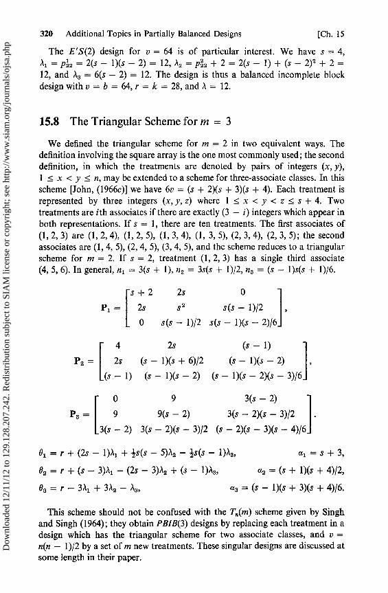
320 Additional Topics in Partially Balanced Designs [Ch. 15
The E'S(2) design for v = 64 is of particular interest. We have s = 4,,11=P22= 2(s - 1)(s-2)= 12, A2=p22+2= 2(s- 1)+(s-2) 2 +2=12, and A3 = 6(s - 2) = 12. The design is thus a balanced incomplete blockdesign with v = b = 64, r = k = 28, and ^1 = 12.
15.8 The Triangular Scheme for m = 3
We defined the triangular scheme for m = 2 in two equivalent ways. Thedefinition involving the square array is the one most commonly used; the seconddefinition, in which the treatments are denoted by pairs of integers (x, y),1 < x < y < n, may be extended to a scheme for three-associate classes. In thisscheme [John, (1966c)] we have 6v = (s + 2)(s + 3)(s + 4). Each treatment isrepresented by three integers (x, y, z) where 1 < x <y < z < s + 4. Twotreatments are ith associates if there are exactly (3 - i) integers which appear inboth representations. If s = 1, there are ten treatments. The first associates of(1, 2, 3) are (1, 2, 4), (1, 2, 5), (1, 3, 4), (1, 3, 5), (2, 3, 4), (2, 3, 5); the secondassociates are (1, 4, 5), (2, 4, 5), (3, 4, 5), and the scheme reduces to a triangularscheme for m = 2. If s = 2, treatment (1, 2, 3) has a single third associate(4, 5, 6). In general, n l = 3(s + 1), n 2 = 3s(s + 1)/2, n3 = (s - 1)s(s + 1)/6.
s+2 2s
P1 = 2s s2
0 s(s - 1)/2
4 2s
Pz = 2s (s - 1)(s + 6)/2
(s - 1) (s - 1)(s - 2)
0
s(s - 1)/2
s(s - 1)(s - 2)/6
(s - 1)
(s - 1)(s - 2)
(s - 1)(s - 2)(s - 3)/6
0 9 3(s-2)
P3 = 9 9(s - 2) 3(s - 2)(s - 3)/2
3(s - 2) 3(s - 2)(s - 3)/2 (s - 2)(s - 3)(s - 4)/6
61 =r+(2s-l)\ l +- s(s -5)A2 --s(s-1)13 , al=s+3,
02 = r + (s - 3)A l - (2s - 3)12 + (s - 1)A3 , a2 = (s + 1)(s + 4)/2,
63 =r-31 1 +3A2 -23 , a3=(s-1)(s+3)(s+4)/6.
This scheme should not be confused with the T(m) scheme given by Singhand Singh (1964); they obtain PBIB(3) designs by replacing each treatment in adesign which has the triangular scheme for two associate classes, and v =n(n - 1)/2 by a set of m new treatments. These singular designs are discussed atlome length in their paper.
Dow
nloa
ded
12/1
1/12
to 1
29.1
28.2
07.2
42. R
edis
trib
utio
n su
bjec
t to
SIA
M li
cens
e or
cop
yrig
ht; s
ee h
ttp://
ww
w.s
iam
.org
/jour
nals
/ojs
a.ph
p
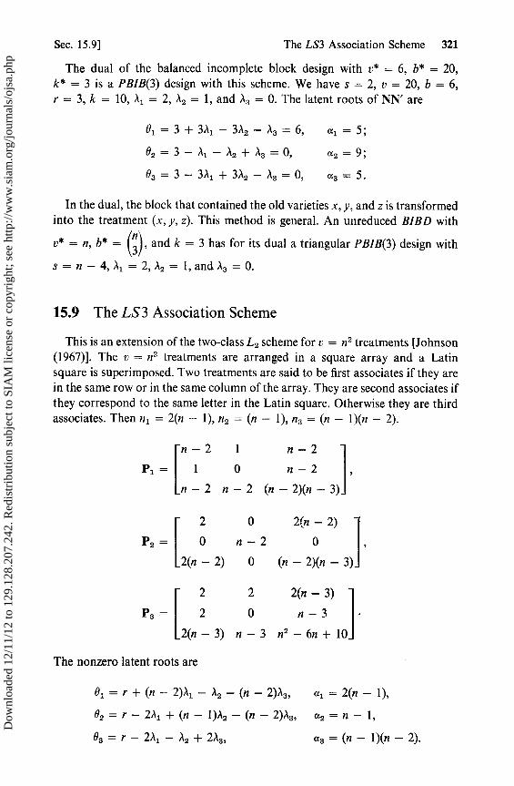
Sec. 15.9] The LS3 Association Scheme 321
The dual of the balanced incomplete block design with v* = 6, b* = 20,k* = 3 is a PBIB(3) design with this scheme. We have s = 2, v = 20, b = 6,r = 3, k = 10, A l = 2, A2 = 1, and d3 = 0. The latent roots of NN' are
81 =3+31 1 -3A2 —A3 =6, a=5;
a2 =9;82 =3— d1 —a2 +a3 =0, a2 =9;
93 = 3 — 3A1 + 32 2 — Á3 = 0, a3 =5.
In the dual, the block that contained the old varieties x, y, and z is transformedinto the treatment (x, y, z). This method is genera]. An unreduced BIBD with
v* = n, b* = (n), and k = 3 has for its dual a triangular PBIB(3) design with
s = n —4,A l =2,,12 = 1, and A„=0.
15.9 The LS3 Association Scheme
This is an extension of the two-class L2 scheme for v = n2 treatments [Johnson(1967)]. The v = n 2 treatments are arranged in a square array and a Latinsquare is superimposed. Two treatments are said to be first associates if they arein the same row or in the same column of the array. They are second associates ifthey correspond to the same letter in the Latin square. Otherwise they are thirdassociates. Then n l = 2(n — 1), n2 = (n — 1), n 3 = (n — 1)(n — 2).
n-2
1 n-2
P1 = 1
0 n-2
n-2 n-2 (n-2)(n-3)
2
0 2(n-2)
P2 = 0
n-2 0
2(n — 2) 0 (n — 2)(n — 3)
2 2 2(n-3)
P3 = 2 0 n-3
2(n-3) n-3 n2 -6n+10
The nonzero latent roots are
0 1 =r +(n-2)A 1 —A2 —(n-2)A3 , a1 = 2(n-1),
62 =r-2Â1 +(n— 1)Â2 —(n-2)113, a2 =n— 1,
B3 = r — 2A, — íA, + 2A , a3 = (n — 1)(n — 2).
Dow
nloa
ded
12/1
1/12
to 1
29.1
28.2
07.2
42. R
edis
trib
utio
n su
bjec
t to
SIA
M li
cens
e or
cop
yrig
ht; s
ee h
ttp://
ww
w.s
iam
.org
/jour
nals
/ojs
a.ph
p
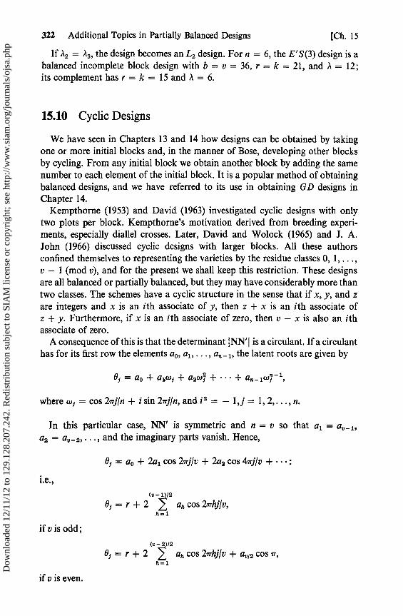
322 Additional Topics in Partially Balanced Designs [Ch. 15
If A2 = a3 , the design becomes an L 2 design. For n = 6, the E'S(3) design is abalanced incomplete block design with b = v = 36, r = k = 21, and A = 12;its complement has r = k = 15 and A = 6.
15.10 Cyclic Designs
We have seen in Chapters 13 and 14 how designs can be obtained by takingone or more initial blocks and, in the manner of Bose, developing other blocksby cycling. From any initial block we obtain another block by adding the samenumber to each element of the initial block. It is a popular method of obtainingbalanced designs, and we have referred to its use in obtaining GD designs inChapter 14.
Kempthorne (1953) and David (1963) investigated cyclic designs with onlytwo plots per block. Kempthorne's motivation derived from breeding experi-ments, especially diallel crosses. Later, David and Wolock (1965) and J. A.John (1966) discussed cyclic designs with larger blocks. All these authorsconfined themselves to representing the varieties by the residue classes 0, 1, ...,v — 1 (mod v), and for the present we shall keep this restriction. These designsare all balanced or partially balanced, but they may have considerably more thantwo classes. The schemes have a cyclic structure in the sense that if x, y, and zare integers and x is an ith associate of y, then z + x is an ith associate ofz + y. Furthermore, if x is an ith associate of zero, then v — x is also an ithassociate of zero.
A consequence of this is that the determinant NN' is a circulant. If a circulanthas for its first row the elements ao, al , ... , an _ 1i the latent roots are given by
6r = ao + abw; + a2u,1 +... + a,ti _ lwf - 1 ,
where w1 = cos 2iij/n + i sin 21Tj/n, and j2 = — 1,j = 1,2,. . . , n.
In this particular case, NN' is symmetric and n = v so that al =a2 = a„ - 2, ..., and the imaginary parts vanish. Hence,
Bj = ao + 2a1 cos 2irj/v + 2a2 cos 4iij/v + • • • :
i.e.,
(v-1)12Bi = r + 2 1 ah cos 27rhj/v,
h=1
ifvisodd;
(v -2)12B1 = r + 2 1 ah cos 27rhj/v + a„12 cos ir,
h=1
if v is even.
Dow
nloa
ded
12/1
1/12
to 1
29.1
28.2
07.2
42. R
edis
trib
utio
n su
bjec
t to
SIA
M li
cens
e or
cop
yrig
ht; s
ee h
ttp://
ww
w.s
iam
.org
/jour
nals
/ojs
a.ph
p
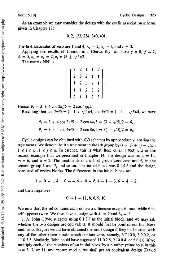
Sec. 15.10] Cyclic Designs 323
As an example we may consider the design with the cyclic association schemegiven in Chapter 12:
012, 123, 234, 340, 401.
The first associates of zero are 1 and 4, al = 2, a2 = 1, and r = 3.Applying the results of Connor and Clatworthy, we have y = 0, S = 2,
0= 5, a1 =a, =2, 0i =(3 ± 1/5)/2.The matrix NN' is
3 2 1 1 2
2 3 2 1 1
1 2 3 2 1.
1 1 2 3 2
2 1 1 2 3
Hence, df = 3 + 4 cos 2ij/5 + 2 cos 47rj/5.Recalling that cos 21T/5 = (- 1 + x/5)/4, cos 4ir/5 = (-1 - \/5)/4, we have
01 = 3 + 4 cos 2ir/5 + 2 cos 4r/5 = (3 + \/5)/2 = 0 4 ,
02 = 3 + 4 cos 47r/5 + 2 cos 87x/5 = 3( - V5)/2 = 03 .
Cyclic designs can be obtained with GD schemes by appropriately labeling thetreatments. We denote thejth treatment in the ith group by (i - 1) + (j - 1)m,1 < i < m, 1 < j < n. In essence, this is what Bose et al. (1953) did in thesecond example that we presented in Chapter 14. The design was for v = 12,m = 6, and n = 2. The treatments in the first group were zero and 6, in thesecond group 1 and 7, and so on. The initial block was 0 1 4 6 and the design,consisted of twelve blocks. The differences in the initial block are
1-0=1,4-0=4,6-0=6,4-1=3,6-4=2,
and their negatives
0-1=11,8,6,9,10.
We note that the set contains each nonzero difference except 6 once, while 6 it-self appears twice. We thus have a design with al = 2 and X12 = 1.
J. A. John (1966) suggests using 0 13 7 as the initial block, and we may askwhether the two designs are equivalent. It should first be pointed out that Boseand his colleagues would have obtained the same design if they had started withany of the other three blocks which contain zero, namely, 6 7 10 0, 8 9 0 2, or11 0 3 5. Similarly, John could have suggested 11 0 2 6, 9 10 0 4, or 5 6 8 0. If wemultiply each of the members of an initial block by a number prime to v, in thiscase 5, 7, or 11, and reduce mod v, we shall get an equivalent design [David
Dow
nloa
ded
12/1
1/12
to 1
29.1
28.2
07.2
42. R
edis
trib
utio
n su
bjec
t to
SIA
M li
cens
e or
cop
yrig
ht; s
ee h
ttp://
ww
w.s
iam
.org
/jour
nals
/ojs
a.ph
p

324 Additional Topics in Partially Balanced Designs [Ch. 15
(1963)], inasmuch as our action will amount only to a relabeling of the treat-ments. In each case, 6 will remain unchanged. Similarly, if we replaced eachtreatment by its negative (mod v), we should get an equivalent design. Multiply-ing 0 1 4 6 by 5 gives 0 5 8 6, which is the fourth of the possible initial blocks inJohn's design. Thus the two designs are equivalent.
Cyclic designs with the hierarchic group divisible scheme can be obtainedby labeling the jth treatment in the ith subgroup of the hth group as
h — 1 + (i — 1)N1 + (j — l)N1 N2 .
With this labeling, a design with Nl = N2 = N3 = 2 would have varieties 0, 2and 4, 6 in the subgroups of the first group and 1, 3 and 5, 7 in the other group.The E'S(l) design is now the cyclic design generated by 0 1 3 5 7. The ES(1)design is also cyclic and consists of the two blocks 0 2 4 6 and 1 3 5 7, eachrepeated four timer. The pair of blocks is called a partial cycle.
15.11 Generalized Cyclic Designs
We may generalize the concept of a cyclic design by allowing the varieties to beelements of an Abelian group under addition. As before, it is convenient to takethe initial block to contain the identity zero. The jth block is then obtained byadding the jth element of the group to each member of the initial block. Again,several initial blocks may be used, and partial cycles may be included.
For group divisible designs we may use a double modulus system, representingthe jth treatment in the ith group by the ordered pair ij; addition is then definedby gh + ij= xy where x - g + i (mod m) and y - h + j (mod n), and thesame system can be used for L2 designs. Consider, for example, the array of ninetreatments
00 01 0210 11 1220 21 22,
with arithmetic for both coordinates being mod 3.We can consider the array as a GD scheme with rows as groups. Then the
initial block 00 01 0211 generates a GD design with A l = 3 and A2 = 1. Con-sidering the array as an L 2 scheme, the initial block 00 01 12 22 generates theES(l) design with A l = 1 and A2 = 2.
We can also use this labeling of treatments for the rectangular scheme.Suppose we take a scheme with m = 2 and n = 3.
00 01 0210 11 12.
Arithmetic for the first digit is mod 2, and for the second digit mod 3. Then theinitial block 00 11 12 gives the E'S(3) design with Al = 1, Aa = 0, and a3 = 2.
Dow
nloa
ded
12/1
1/12
to 1
29.1
28.2
07.2
42. R
edis
trib
utio
n su
bjec
t to
SIA
M li
cens
e or
cop
yrig
ht; s
ee h
ttp://
ww
w.s
iam
.org
/jour
nals
/ojs
a.ph
p

Sec. 15.12] Designs for Eight Treatments in Blocks of Three 325
In the cubic scheme, the coordinate system is immediately adaptable to cyclicdesigns. We give two examples for the schemes with v = 27 and v = 64.
In the scheme for v = 27, we denote the treatments by 000, 001, and so on,with arithmetic mod 3. Consider the design generated by the initial block000, 001, 002. The six differences are 001 and 002, each repeated three times.The twenty-seven blocks consist of a partial cycle of nine blocks repeated threetimes. Suppose now that we take the set of three initial blocks, 000, 001, 002; 000,010, 020; 000, 100, 200, and take one partial cycle from each set of blocks. Theresulting design will have b = v = 27, r = k = 3, ,1 1 = 1, X12 = 0, and X13 = 0.
In a similar way, partial cycles from the six initial blocks 000, 012, 021;000, 011, 022; 000, 102, 201; 000,101,202; 000, 120, 210; 000, 110, 220 giveb = 54, r = 6, k = 3, A, = 0, "2 = 1, and A3 = 0. The initial blocks 000, 111,222; 000, 112, 221; 000,121,212; 000, 211, 112 likewise give a design withb = 36, r = 4, A l = = 0, and A 3 = 1, and all three of these PBIB(3) designscombined form a BIBD with b = 117, k = 3, r = 13, A = 1.
For v = 64 we can use for the coordinates the elements of the Galois fieldGF(22), namely, 0, 1, x, and 1 + x, which we write as y. We can obtain asimilar set of designs with k = 4 and other parameters:
(i) b =48, r=3, ,1 1 =1, 2 =0, A3 =0;(ii) b = 144, r = 9, X1 1 =0, 2 =1, A3 =0;(iii) b = 144, r = 9, A, = 0, A2 = 0, ,1 3 = 1.
In design (iii), one of the initial blocks used is 000, 111, xxx, yyy. The differ-ences are 111, xxx, yyy, xxx - 111 = yyy, yyy - 111 = xxx, yyy - xxx =111 and their negatives; but sine all arithmetic is mod 2, taking the negativesamounts to repeating each difference again. The set of twelve differences is thus111, xxx, and yyy, each appearing four times. The actual design consists ofpartial cycles (sixteen blocks) on each of the following nine initial blocks:
000, 111, xxx, yyy; 000, 11x, xxy, yyl; 000, ily, yyx, xxl;
000, lxl, xyx, yly; 000, lyl, yxy, xlx; 000, xl 1, l yy, yxx;
000, yl 1, xyy, lxx; 000, lxy, xyl, yxl ; 000, lyx, yxl, .xly.
15.12 Designs for Eight Treatments in Blocks of Three
As an illustration of the techniques that have been developed so far, we con-sider designs with v = 8 and k = 3. In particular, we shall look at designs withtwo or three associate classes. We have the following possible schemes:
(i) GD with m = 2, n = 4, and ordering 0 24 6, 1 3 5 7;(ii) GD with m = 4, n = 2, and ordering 04, 15, 26, 37;(iii) Hierarchic GD with ordering 04, 26, 15, 37;(iv) Rectangular;(v) Cubic.
Dow
nloa
ded
12/1
1/12
to 1
29.1
28.2
07.2
42. R
edis
trib
utio
n su
bjec
t to
SIA
M li
cens
e or
cop
yrig
ht; s
ee h
ttp://
ww
w.s
iam
.org
/jour
nals
/ojs
a.ph
p

326 Additional Topics in Partially Balanced Designs [Ch. 15
For v = 8, the last two schemes are equivalent.We turn first to the ordinary cyclic designs with a single initial block. Each
initial block consists of zero and two other treatments. There are thus (2) = 21
possible initial blocks, but they occur in equivalence sets. /Consider the block 0, 1, 2. When we cycle on it, we obtain 0 1 7, 0 6 7, and so
these three blocks are equivalent in the sense that they generate the same design.Furthermore, multiplying by 3 gives 0 3 6, 0 3 5, 0 2 5, and we have one equiva-lence set with six triples. The initial block 01 3 also gives us 0 2 7, 0 5 6, withdifferences 1 - 0, 3 - 0, 3 - 1, and their negatives. We could as wel] haveconsidered the negative of the block, replacing 1 by 7 and 3 by 5 to give 0 5 7, and,similarly, 01 6, 0 2 3, for another set of six. There are two more equivalence sets,01 4,037,045,047,01 5,034,andthesetofthreetriples,024,026,046.For designs with a single initial block, we need therefore consider only the fourcases:
(i) 01 2, with differences 1, 1, 2, 6, 7, 7 [or, as David (1963) writes, (1 2, 2)];this gives four associate classes, with the associates of zero being 1, 7;2, 6; 3, 5;4,andAl =2,A2 = 1, 13 =A4 =0;
(ii) 01 3, which gives a GD design with groups 0, 4; 1, 5; 2, 6; 3, 7 andAr =0, ,12 =1;
(iii) 014, which gives a hierarchic GD design with ,11 = 1, Aa = 0, ,13 = 2;and
(iv) 024, which gives a disconnected GD design with m = 2, n = 4, and=2,A2 =0.
J. A. John (1966) also considers combinations of several initial blocks. Theset (0 1 2), (0 1 3), (014) gives a design for four classes; al = 4, A2 = As =A4 = 2. There are three other designs with three associate classes, all of whichhave the hierarchic scheme. They are generated by
(0 1 3), (0 2 4) Jol = 1, A2 = 3, A3 = 2;
(0 1 3), (014) Al = 2, A2 = 1, A3 = 2;
(0 1 3), (014), (0 2 4) Al = 2, ,1a = 3, A3 = 4
We can obtain three more designs by using the cubic scheme for v = 8.Denoting the treatments by 000, 001, 010, and so on, with arithmetic mod 2, theinitial blocks and values of A, are
(000, 001, 010), (000, 010, 100), (000, 100, 001) A1 = 4, A2 = 2, A3 = 0;
(000, 001, 110), (000, 010, 101), (000, 100, 011) X11 = A2 = 2, As = 6;
(000, 011, 110) X11 = a3 = 0, ,1z = 2.
Dow
nloa
ded
12/1
1/12
to 1
29.1
28.2
07.2
42. R
edis
trib
utio
n su
bjec
t to
SIA
M li
cens
e or
cop
yrig
ht; s
ee h
ttp://
ww
w.s
iam
.org
/jour
nals
/ojs
a.ph
p

Exercises 327
15.13 Conclusion
The construction of designs and the discovery of new schemes remains afertile field for research, and in this chapter we have given only a limited surveyof the field. It might, however, be appropriate to recall the last pages of Chapter12 in which it was suggested that from a practical standpoint there is sometimeslittle to choose between the various alternative designs that can be used in someproblems. We mentioned at that time the nineteen designs that J. A. John listedfor v = 12 and k = 4, with efficiencies ranging from 0.8007 to 0.8166, themaximum being attained by a GD design. The mathematical problems dis-cussed in the last three chapters are very interesting from a theoretical point ofview and have a fascination for pure mathematicians as well as for statisticians.
In spite of the beauty and elegance of the mathematical results, the practicingstatistician should stil) bear in mind that the more complex the design, the easierit is for something to go wrong. We conclude with the maxim that has alreadyappeared at the end of Chapter 12: When you design an experiment, keep it assimple as you can.
Exercises
1. Find the latent roots of NN' and their multiplicities for the triangular designs.2. Find the latent roots of NN' and their multiplicities for designs with the L(n)
scheme.3. Verify the results given for the latent roots of NN' and their multiplicities for the
several three-associate class schemes.4. The hierarchic GD design is obtained from a GD design by replacing each
treatment by a set of N3 new treatments. We may similarly take an L(n) schemeand replace each treatment by a group of m new treatments. Two treatments aresaid to be first associates if they belong to the same group, and second associatesif their groups correspond to first associates in the L(n) scheme. This is theL,(n, m) scheme of Singh and Singh (1962). Find the P matrices, the latent rootsof NN', and their multiplicities for this scheme.
5. (Continuation) They also defined in the same paper the T(m) scheme, in whichthey take a triangular scheme and replace each treatment by a group of m newtreatments. The three associate classes are defined as for the L,(n, m) scheme.Derive the P matrices, the latent roots of NN', and their multiplicities for thisscheme.
6. Show that if in a PBIB(2) design 0 is not a perfect square then
P21 = P12 = Pi = t, nt = na = al = a2 = 2t, v = 4t + 1.
7. Show that if v = 4t + 1 and v is a prime we may obtain a cyclic associationscheme by taking as the first associates of zero either the set of quadraticresidues of v or its complement; the first associates of i are then obtained byadding i to each of the first associates of zero.
Dow
nloa
ded
12/1
1/12
to 1
29.1
28.2
07.2
42. R
edis
trib
utio
n su
bjec
t to
SIA
M li
cens
e or
cop
yrig
ht; s
ee h
ttp://
ww
w.s
iam
.org
/jour
nals
/ojs
a.ph
p

328 Additional Topics in Partially Balanced Designs [Ch. 15
8. (Continuation) Obtain a similar result when v = 9 or 25 by allowing the treat-ments to be the elements of the Galois field of v elements.
9. Show that for a PBIB(2) scheme vn1n2 = 1a1 a2 [Mesner (1965)].10. Show that a necessary and sufficient condition for a PBIB(2) scheme to have « 1
and a2 equal in some order to nl and n2 is that the scheme be of the pseudo-cyclic, the pseudo-Latin square or the NL types [Mesner (1967)].
11. Prove the following results for designs with the rectangular scheme:
(i) If 0 = 0, k is divisible by n and each block contains exactly kin treatmentsfrom each column of the array;
(ii) If 02 = 0, k is divisible by m and each block contains kim treatments fromeach row;
(iii) If 0 = Bz = 0, there are k(r — 1)/(b — 1) treatments common to any twoblocks of the design [Vartak (1959)].
12. Show that there are only five nonisomorphic cyclic designs with v = b = 8 andr = k = 4 and a single initial block.
13. Show that although the cyclic design for v = 8 generated by (0,. 1, 2, 4) has onlytwo distint values of a,, nevertheless there are four associate classes.
14. Prove that cos(27T/5) = (— 1 + x/5)/4.
Dow
nloa
ded
12/1
1/12
to 1
29.1
28.2
07.2
42. R
edis
trib
utio
n su
bjec
t to
SIA
M li
cens
e or
cop
yrig
ht; s
ee h
ttp://
ww
w.s
iam
.org
/jour
nals
/ojs
a.ph
p
Appendix
A.1 Matrices
We review in this appendix some properties of matrices, vector spaces, andquadratic forms. The elements of all the matrices will be real numbers, and someof the results given are not true without this restriction. Some of the results willbe proved as theorems; others will be stated without proof, and some of thesewill appear later as exercises. Although it is reasonable to assume that moststudents entering a graduate course in the mathematical theory of design ofexperiments will have had some exposure to elementary matrix theory, manyundergraduate courses in linear algebra do not progress as far as the discussionof quadratic forms, which are essential to the development of our subject. Thisdoes not attempt to be a complete presentation, and the reader is referred forfurther details to the standard texts. Some basic results about determinants willbe assumed.
A matrix, in the context in which we shall be considering them, is a rectangulararray of elements, which in our case will be real numbers (or, at a later stage,smaller matrices of real numbers). We talk of a matrix A having m rows and ncolumns, sometimes written (m x n), and denote by ai, the element in the ithrow and the jth column. We shall use boldface type, A, to denote matrices and weshall write A = (a). A square matrix with m rows and m columns is said to be oforder m. If a{5 = a;; , A is called symmetrie. 0 will denote a matrix of zero ele-ments. I, is the identity matrix, the square matrix of order n with ones along themain diagonal and zeros elsewhere, i.e., a„ = 1, a,; = 0, i j. If there is nodanger of confusion, we shall omit the subscript n and write I.
329
Dow
nloa
ded
12/1
1/12
to 1
29.1
28.2
07.2
42. R
edis
trib
utio
n su
bjec
t to
SIA
M li
cens
e or
cop
yrig
ht; s
ee h
ttp://
ww
w.s
iam
.org
/jour
nals
/ojs
a.ph
p

330 Appendix
A matrix A can be multiplied by a scalar (a real number) c. The product isdefined as cA = B where b,1 = caii .
Two matrices A and B, each with m rows and n columns, can be added.Addition is defined by A + B = C where c sj = a,, + bi,.
The product AB of two matrices is defined only if the number of columns of Ais the same as the number of rows of B, in which case we define AB = C whereCt, = Ik a1kbkl. In general it is not true that AB = BA; indeed, one product mayexist and the other not. If AB = BA, the two matrices are said to commute.
The transpose of a matrix A with m rows and n columns will be written as A'.Some authors write AT. It is defined as A' = C where C has n rows and mcolumns and c, 1 = a51 . If A and B are two matrices such that AB exists, then(AB)' = B'A'.
So far as we are concerned, a vector of n elements may be considered as amatrix with n rows and a single column. Its transpose is sometimes called arow vector. We shall use 1,, to denote a vector of n unit elements. Em„ willdenote a matrix of m rows and n columns with every element unity: Em,,,1,,,i. We shall usually write J„ for E,a , n. The length of a vector y is defined as dwhere d2 = y'y = 1 y. Two vectors, x and y, are said to be orthogonal ifx'y = y'x = 0; this implies that x and y have the same number of elements.
Consider a set of vectors y l , ... , ym , each with n elements. They are said to belinearly independent if there exists no set of scalars Cl, ..., Cm (except the setC1 = • • • = cm = 0) for which 1 ciyi = 0 where 0 is a vector of zero elements.Otherwise, we have a linearly dependent set. The zero vector 0 is itself a linearlydependent set. The collection of all linear combinations c {yi is called the vectorspace, V, spanned by the set of vectors y i , ..., ym. If the set yl , ..., ym is alinearly dependent set, Vis also spanned by a subset of y l , ... , Y. This leads usto the idea of a basis for a vector space. We define a basis (or a Hamel basis) for avector space V to be a set of linearly independent vectors that span V. It can beshown that every vector space has a basis and that all bases for a given vectorspace contain the same number of vectors. This number is called the dimensionof the space. It is closely connected with the next concept, that of the rank of amatrix. We may consider a matrix A, (m x n), as a collection of n columns orvectors.
The rank of A, written r(A), is the number of linearly independent columns inA, which is the same as the dimension of the vector space spanned by thecolumns of A. It can be shown that this is the same as the number of linearlyindependent rows of A, and that r(A) is equal to the order of the largest non-vanishing determinant that can be formed from the columns and the rows of A.It follows that r(A) < min(m, n), and that r(0) = 0. We conclude these pre-liminaries by defining the inverse of a matrix and proving some theorems aboutthe ranks of matrices.
Let A be a square matrix, and let Al be the determinant with elements a is .If Al = 0, A is said to be singular; if IAI 0 0, A is nonsingular. Let A,f denotethe cofactor of the element a,i in Al; A,j is the value of the determinant obtainedby striking out the ith row and the jth column of A, multiplied by (-1)'+'
Dow
nloa
ded
12/1
1/12
to 1
29.1
28.2
07.2
42. R
edis
trib
utio
n su
bjec
t to
SIA
M li
cens
e or
cop
yrig
ht; s
ee h
ttp://
ww
w.s
iam
.org
/jour
nals
/ojs
a.ph
p

Appendix 331
Suppose now that A is nonsingular, and consider the matrix C = (c, j) wherec{1 = AjJ1Al. It follows from elementary properties of determinants, namely1 a 1A,f = ^Al and I; akJA {f = 0 where i k, that AC = CA = I. C is calledthe inverse of A and is written as A -1 . C is unique, and, if A and B are bothnonsingular, (AB) -' = B - lA -1 . Every square nonsingular matrix A has aninverse. If r(A) is less than the order of A, Al = 0, and A has no inverse.
Theorem. Let A and B be (m x n) matrices. Then r(A + B) < r(A) + r(B).
PROOF. Let a be a set of r(A) linearly independent columns of A, and P a set ofr (B) linearly independent columns of B; let y be the union of the two sets a and /.Every column of C = A + B is a linear combination of the columns of y.Then r(C) is not greater than the number of columns in y, and so r(A + B) <r(A) + r(B). 1
Theorem. Let A and B be matrices such that AB exists. Then r(AB) < r(A) andr(AB) < r(B).
PROOF. The columns of AB are linear combinations of the columns of A. Thusthey belong to the space spanned by the columns of A, and so r(AB) < r(A).Similarly, r(B'A') < r(B'). But r(B'A') = r(AB) and r(B') = r(B) so thatr(AB) < r(B). a
Corollary 1. If A is nonsingular and AB exists, r(AB) = r(B).
PROOF. By the theorem r(AB) < r(B); but B = (A - ')(AB), so that r(B) <_r(AB). Hence, r(AB) < r(B) < r(AB), and so r(AB) = r(B). We may similarlyprove that, if CA exists, r(CA) = r(C). a
Corollary 2. If A and C are nonsingular r(ABC) = r(B), i.e., the rank of a matrixis not changed by multiplying on the left and the right by nonsingular matrices.
Corollary 3. If A and B are square matrices and AB = 0, then A = 0, or B = 0,or else A and B are both singular.
PROOF. Suppose, in contradiction, that A is nonsingular and B 0. Thenr(AB) = r(B) > 0, and AB 0. Similarly, if B is nonsingular and A = 0,AB 0 0. 3
A.2 Orthogonality
We have mentioned that two vectors, x and y, are said to be orthogonal if theproduct x'y = y'x = 0. A set of vectors of unit length which are mutuallyorthogonal is called an orthonormal set. A set of n mutually orthogonal vectors of
Dow
nloa
ded
12/1
1/12
to 1
29.1
28.2
07.2
42. R
edis
trib
utio
n su
bjec
t to
SIA
M li
cens
e or
cop
yrig
ht; s
ee h
ttp://
ww
w.s
iam
.org
/jour
nals
/ojs
a.ph
p
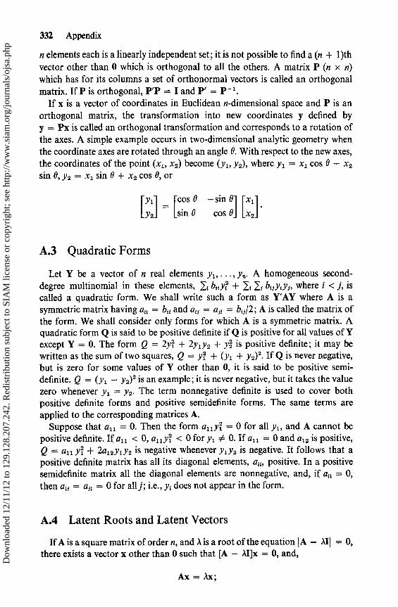
332 Appendix
n elements each is a linearly independent set; it is not possible to find a (n + 1)thvector other than 0 which is orthogonal to all the others. A matrix P (n x n)which has for its columns a set of orthonormal vectors is called an orthogonalmatrix. If P is orthogonal, P'P = I and P' = P -1 .
If x is a vector of coordinates in Euclidean n-dimensional space and P is anorthogonal matrix, the transformation into new coordinates y defined byy = Px is called an orthogonal transformation and corresponds to a rotation ofthe axes. A simple example occurs in two-dimensional analytic geometry whenthe coordinate axes are rotated through an angle 0. With respect to the new axes,the coordinates of the point (x1 , x2) become (y l , y2), where y l = xl cos B — x2
sin 0, Y2 = xl sin 0 + x2 cos 0, or
[y2] [sin B cos 9, [x2,
A.3 Quadratic Forms
Let Y be a vector of n real elements y l , ..., y,,. A homogeneous second-degree multinomial in these elements, l i b;t yi + l i I, bi, y; yf, where i <j, iscalled a quadratic form. We shall write such a form as Y'AY where A is asymmetric matrix having a{, = b;, and a;1 = a;i = b;j/2; A is called the matrix ofthe form. We shall consider only forms for which A is a symmetric matrix. Aquadratic form Q is said to be positive definite if Q is positive for all values of Yexcept Y = 0. The form Q = 2y1 + 2y,y2 + y2 is positive definite; it may bewritten as the sum of two squares, Q = yi + (yl + y2) 2 . If Q is never negative,but is zero for some values of Y other than 0, it is said to be positive semi-definite. Q = (yl — Y2)2 is an example; it is never negative, but it takes the valuezero whenever y l = Y2 . The term nonnegative definite is used to cover bothpositive definite forms and positive semidefinite forms. The same terms areapplied to the corresponding matrices A.
Suppose that a ll = 0. Then the form ailyi = 0 for all y l , and A cannot bepositive definite. If a ll < 0, allyi < 0 for y l 0. Ifall = 0 and a 12 is positive,Q = all Yi + 2a12Y1Y2 is negative whenever y1 y2 is negative. It follows that apositive definite matrix has all its diagonal elements, at,, positive. In a positivesemidefinite matrix all the diagonal elements are nonnegative, and, if a ;i = 0,then = a;, = 0 for all j; i.e., y i does not appear in the form.
A.4 Latent Roots and Latent Vectors
If A is a square matrix of order n, and d is a root of the equation A — M] = 0,there exists a vector x other than 0 such that [A — AI]x = 0, and,
Ax = ^1x;
[y2] [sin B cos 9, [x2,
Dow
nloa
ded
12/1
1/12
to 1
29.1
28.2
07.2
42. R
edis
trib
utio
n su
bjec
t to
SIA
M li
cens
e or
cop
yrig
ht; s
ee h
ttp://
ww
w.s
iam
.org
/jour
nals
/ojs
a.ph
p

Appendix 333
A is called a latent root (or characteristic root or proper value or eigenvalue) ofA, and x is a latent (characteristic, proper or eigen-) vector corresponding to A.Counting multiplicities, there are exactly n roots; if A is symmetrie, the numberof nonzero roots of A is equal to the rank of A. We now confine ourselves tosymmetrie matrices A.
Theorem 1. If X11 , a; are two latent roots of A such that ,\ 0 ,1 j , and x, x; are twocorresponding latent vectors, then x i and x; are orthogonal.
PROOF. We have Ax ; = ,1ixj , Axf = ,1;x1 , so that xj'Ax, = d ixix ; , x,Ax5 = A.xixf .Then, since A is symmetrie, taking the transpose of the Jatter expression givesx;Ax { = 21;x;x,. Thus A;xfx, = Ajxjx t, and since A. # ,1;, x;x t = 0.
It can also be shown that if A is a latent root with multiplicity m, there is a setof exactly m mutually orthogonal latent vectors corresponding to A. We may takethe lengths of the latent vectors to be unity, and thus obtain for A a st of northonormal vectors. Let P denote the matrix whose columns are these ortho-normal vectors; P is orthogonal and
AP = PA,
where A is a diagonal matrix (i.e., a matrix with all its off-diagonal elementszero), having as the diagonal elements the latent roots, each appearing as manytimes as its multiplicity. Multiplying on the left by P' gives P'AP = P'PA = A.We state this result as a theorem.
Theorem 2. Let A be a square symmetrie matrix, and A be the diagonal matrixfust defined. There exists an orthogonal matrix P such that P'AP = A. Con-versely, if there exists an orthogonal matrix P such that P'AP = D where D isdiagonal, the diagonal elements are the latent roots of A.
Since P is nonsingular, r(A) = r(P'AP) = r(A), and we see that the rank of Ais equal to the number of nonzero latent roots, counting their multiplicities.Denote the ith diagonal element of A by Al . Let a diagonal matrix D be con-structed as follows. The ith diagonal element d ij of D = 1 if A l = 0 and -1 /2 ifa, 0. Let Q = PD. Q is not singular. Then the transformation Y = QZchanges Y'AY into 1 ±z{ where the number of positive signs is equal to thenumber of positive latent roots, and the number of negative signs is equal to thenumber of negative latent roots.
If B is a nonsingular matrix we have
B -1Ax = B - 'ABB - ix = B - llx = AB -1x,
so that A is also a latent root of B - 'AB with latent vector B - 'x. The two matricesA and B - 'AB are said to be similar.
Theorem 3. A is positive definite if, and only if, all its latent roots are positive.
Dow
nloa
ded
12/1
1/12
to 1
29.1
28.2
07.2
42. R
edis
trib
utio
n su
bjec
t to
SIA
M li
cens
e or
cop
yrig
ht; s
ee h
ttp://
ww
w.s
iam
.org
/jour
nals
/ojs
a.ph
p
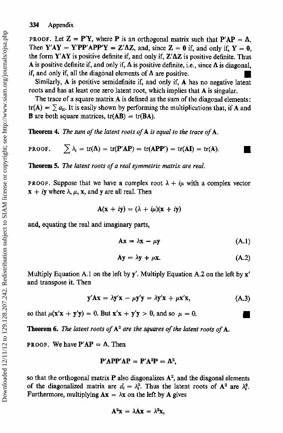
334 Appendix
PROOF. Let Z = P'Y, where P is an orthogonal matrix such that P'AP = A.Then Y'AY = Y'PP'APP'Y = Z'AZ, and, since Z = 0 if, and only if, Y = 0,the form Y'AY is positive definite if, and only if, Z'AZ is positive definite. ThusA is positive definite if, and only if, A is positive definite, i.e., since A is diagonal,if, and only if, all the diagónal elements of A are positive. 3
Similarly, A is positive semidefinite if, and only if, A has no negative latentroots and has at least one zero latent root, which implies that A is singular.
The trace of a square matrix A is defined as the sum of the diagonal elements:tr(A) = 1 a, i . It is easily shown by performing the multiplications that, if A andB are both square matrices, tr(AB) = tr(BA).
Theorem 4. The sum of the latent roots of A is equal to the trace of A.
PROOF. d, = tr(A) = tr(P'AP) = tr(APP') = tr(AI) = tr(A).
Theorem 5. The latent roots of a real symmetric matrix are real.
PROOF. Suppose that we have a complex root ,A + iµ with a complex vectorx + iy where , , µ, x, and y are all real. Then
A(x + iy) = (,1 + iµ)(x + iy)
and, equating the real and imaginary parts,
Ax=Ax—µy (A.1)
Ay = Ay + µx. (A.2)
Multiply Equation A. 1 on the left by y'. Multiply Equation A.2 on the left by x'and transpose it. Then
y'Ax = Ay'x — uy'y = Ay'x + µx'x, (A.3)
so that µ(x'x + y'y) = 0. But x'x + y'y > 0, and so µ = 0. a
Theorem 6. The latent roots of Aa are the squares of the latent roots of A.
PROOF. We have P'AP = A. Then
P'APP'AP = P'A2P = A2 ,
so that the orthogonal matrix P also diagonalizes A 2, and the diagonal elementsof the diagonalized matrix are d, = A. Thus the latent roots of A 2 are Aa.Furthermore, multiplying Ax = Ax on the left. by A gives
A2x = AAx = A2x,
Dow
nloa
ded
12/1
1/12
to 1
29.1
28.2
07.2
42. R
edis
trib
utio
n su
bjec
t to
SIA
M li
cens
e or
cop
yrig
ht; s
ee h
ttp://
ww
w.s
iam
.org
/jour
nals
/ojs
a.ph
p

Appendix 335
and we see that each vector x corresponding to a root ,1 of A also corresponds toa root A2 of A2 .
The following theorem is of particular use to us.
Theorem 7. Let X be a real matrix with m rows and n columns. Then X'X isnonnegative definite and r(X'X) = r(X).
PROOF. Since X'X is symmetric, there is an orthogonal P such that P'X'XP = A.Let B = (b if) = XP. Then B'B = A, and we have, writing the columns of B asvectors, b i , bbi = a, and babi = 0 where i # j. It follows that A, = 0 if and onlyif b, = 0; otherwise, > 0. Thus the latent roots are nonnegative and X'X isnonnegative definite.
The vectors b, are mutually orthogonal. The rank of X'X is equal to thenumber of positive diagonal elements of A, which, in turn, is the number of b $
that are not 0. Thus, r(X'X) = r(B) = r(XP) = r(X). EWe state without proof the following theorem, which is to be found in many
of the standard textbooks.
Theorem 8. A necessary and sufficient condition for A to be positive definite is thatevery principal minor of IAI shall be positive. A principal minor of Al is thedeterminant of a submatrix of A obtained by striking out some rows of A and thecorresponding columns so that the diagonal elements of the submatrix are alsodiagonal elements of A.
A square symmetric matrix A is said to be idempotent if Al = A. The followingproperties of idempotent matrices are readily established:
(i) A necessary and sufficient condition for A to be idempotent is that thelatent roots of A are either zero or one;
(ii) If A is idempotent, r(A) = tr(A);(iii) If A is idempotent and Q is orthogonal, Q'AQ is idempotent;(iv) If A is idempotent and a{, = 0, then ajj = af, = 0 for all j;(v) If A is idempotent, a,ll its diagonal elements are nonnegative.
A.5 Simultaneous Linear Equations
We conclude this discussion of matrices by recalling some results about thesolution of sets of simultaneous linear equations.
Consider the set of linear equations Ax = b where A has m rows and ncolumns, and suppose that we wish to solve for x. If m = n, and r(A) = n, thesolution vector is x = A - 'b. Otherwise, there are three possibilities to beconsidered:
(i) There is no solution;(ii) There is an infinite number of solution vectors;
(iii) There is a unique solution vector.
Dow
nloa
ded
12/1
1/12
to 1
29.1
28.2
07.2
42. R
edis
trib
utio
n su
bjec
t to
SIA
M li
cens
e or
cop
yrig
ht; s
ee h
ttp://
ww
w.s
iam
.org
/jour
nals
/ojs
a.ph
p

336 Appendix
For example, we may have the following four equations in two unknowns:
x1 + x2 = 3 (A.4)
xl + 2x2 = 4 (A.5)
2x1 + 3x2 = 7 (A.6)
2x1 + 3x2 = 8. (A.7)
Equation A.4 alone admits an infinity of solutions; we may take any number tthat we wish and obtain the solution vector x' = (t, 3 — t).
The pair of equations A.4 and A.5 has the unique solution vector x' = (2, 1).The addition of equation A.6 makes no difference because it is actually just thesum of Equations A.4 and A.5. When, however, Equation A.7 is included we havean inconsistent set; subtracting Equation A.6 from Equation A.7 would give0=1.
We state the following results without proof. B is the augmented matrix(A, b), i.e., the matrix A with the column b added to it. A set of equations is raidto be consistent if it has at least one solution.
A necessary and sufficient condition for the equations to be consistent is thatr(A) = r(B). If r(A) = r(B) = n, there is a unique solution vector; if r(A) =r(B) < n, then there is an infinity of solutions and n — r(A) of the xi may beassigned arbitrarily.
Exercises
The exercises involve the derivation of some results stated without proof in thetext. A denotes a square symmetric matrix of order n with real elements. C is anymatrix with real elements.
1. Show directly that (AC)' = C'A'.2. All bases for a given finite dimensional vector space have the same number of
vectors.3. Let V„ be the space of all vectors in En (Euclidean n space). The dimension of
V. is n.4. There does not exist a set of n + 1 mutually orthogonal vectors in V.5. The rank of A is the order of the largest nonvanishing determinant in A.6. The number of linearly independent rows of C is the same as the number of
linearly independent columns of C.7.A -1 is unique. If B is a right inverse of A and E is a right inverse, then B = E.
If B and E are both left inverses, B = E. We have given in the text a procedurefor obtaining one matrix that is both a right and left inverse of A when A isnonsingular.
8. We defined latent roots as solutions of IA — Al] = 0. Show that any scalar ,1 forwhich there exists a vector x ; 0 such that Ax = Ax is a root of JA — tIj = 0.
Dow
nloa
ded
12/1
1/12
to 1
29.1
28.2
07.2
42. R
edis
trib
utio
n su
bjec
t to
SIA
M li
cens
e or
cop
yrig
ht; s
ee h
ttp://
ww
w.s
iam
.org
/jour
nals
/ojs
a.ph
p

Appendix 337
9. If A is a latent root of A with multiplicity m, show that we can find a set of mmutually orthogonal latent vectors (but no more) corresponding to A.
10. A is positive semidefinite if, and only if, A has at least one zero latent root and nonegative latent roots.
11. tr(BC) = tr(CB).12. If there exists an orthogonal matrix P such that P'AP is diagonal, then
P'AP = A.13. A necessary and sufficient condition for A to be positive definite is that every
principal minor of IAI be positive.14. If A is idempotent and I = A + B, then B is idempotent and AB = BA = 0.15. If the elements of C are real, C'C = 0 if, and only if, C = 0. Show by a counter-
example that this is not true when C has complex elements.
Dow
nloa
ded
12/1
1/12
to 1
29.1
28.2
07.2
42. R
edis
trib
utio
n su
bjec
t to
SIA
M li
cens
e or
cop
yrig
ht; s
ee h
ttp://
ww
w.s
iam
.org
/jour
nals
/ojs
a.ph
p
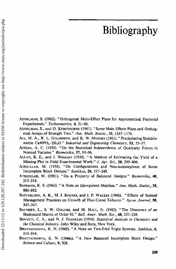
Bibliography
ADDELMAN, S. (1962). "Orthogonal Main-Effect Plans for Asymmetrical FactorialExperiments." Technometrics, 4, 21-46.
ADDELMAN, S., and O. KEMPTHORNE (1961). "Some Main Effects Plans and Orthog-onal Arrays of Strength Two." Ann. Math. Statist., 32, 1167-1176.
AIA, M. A., R. L. GoLDSMITH, and R. W. MOONEY (1961). "Precipitating Stoichio-metric CaHPO4 . 2H20." Industrial and Engineering Chemistry, 53, 55-57.
AITKEN, A. C. (1950). "On the Statistical Independence of Quadratic Forms inNormal Variates." Biometrika, 37, 93-96.
ALLAN, R. E., and J. WISHART (1930). "A Method of Estimating the Yield of aMissing Plot in Field Experimental Work." J. Agr. Sci., 20, 399-406.
ATIQULLAH, M. (1958). "On Configurations and Non-isomorphism of SomeIncomplete Block Designs." Sankhya, 20, 227-248.
ATIQULLAH, M. (1961). "On a Property of Balanced Designs." Biometrika, 48,215-218.
BANERJEE, K. S. (1964). "A Note on Idempotent Matrices." Ann. Math. Statist., 35,880-882.
BATCHELDER, A. R., M. J. ROGERS, and J. P. WALKER (1966). "Effects of SubsoilManagement Practices on Growth of Flue-Cured Tobacco." Agron. Journal, 58,345-347.
BAUMERT, L., S. W. GOLOMB, and M. HALL, Jr. (1962). "The Discovery of anHademard Matrix of Order 92." Bull. Amer. Math. Soc., 68, 237-238.
BENNETT, C. A., and N. J. FRANKLIN (1954). Statistical Analysis in Chemistry andthe Chemical Industry. John Wiley and Sans, New York.
BHATTACHARYA, K. N. (1943). "A Note on Two-Fold Triple Systems. Sankhya, 6,313-314.
BHATTACHARYA, K. N. (1944a). "A New Balanced Incomplete Block Design."Science and Culture, 9, 508.
339
Dow
nloa
ded
12/1
1/12
to 1
29.1
28.2
07.2
42. R
edis
trib
utio
n su
bjec
t to
SIA
M li
cens
e or
cop
yrig
ht; s
ee h
ttp://
ww
w.s
iam
.org
/jour
nals
/ojs
a.ph
p
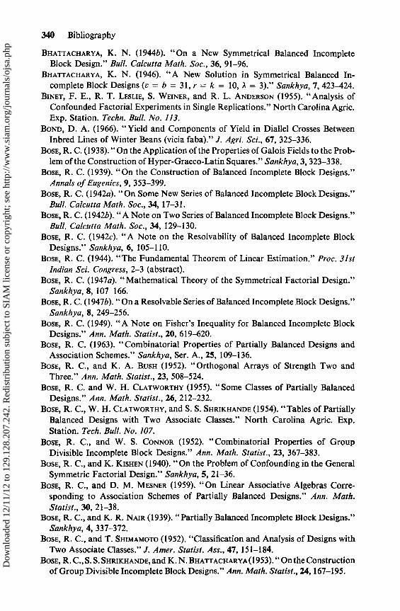
340 Bibliography
BHATTACHARYA, K. N. (1944b). "On a New Symmetrical Balanced IncompleteBlock Design." Bull. Calcutta Math. Soc., 36, 91-96.
BHATTACHARYA, K. N. (1946). "A New Solution in Symmetrical Balanced In-complete Block Designs (v = b = 31, r = k = 10, A = 3)." Sankhya, 7, 423-424.
BINET, F. E., R. T. LESLIE, S. WEINER, and R. L. ANDERSON (1955). "Analysis ofConfounded Factorial Experiments in Single Replications." North Carolina Agric.Exp. Station. Techn. Bull. No. 113.
BOND, D. A. (1966). "Yield and Components of Yield in Diallel Crosses BetweenInbred Lines of Winter Beans (vicia faba)." J. Agri. Sci., 67, 325-336.
BOSE, R. C. (1938). " On the Application of the Properties of Galois Fields to the Prob-lem of the Construction of Hyper-Graeco-Latin Squares." Sankhya, 3, 323-338.
BOSE, R. C. (1939). "On the Construction of Balanced Incomplete Block Designs."Annals of Eugenics, 9, 353-399.
BOSE, R. C. (1 942a). "On Some New Series of Balanced Incomplete Block Designs."Bull. Calcutta Math. Soc., 34, 17-31.
BOSE, R. C. (1942b). "A Note on Two Series of Balanced Incomplete Block Designs."Bull. Calcutta Math. Soc., 34, 129-130.
BOSE, R. C. (1942c). "A Note on the Resolvability of Balanced Incomplete BlockDesigns." Sankhya, 6, 105-110.
BOSE, R. C. (1944). "The Fundamental Theorem of Linear Estimation." Proc. 31stIndian Sci. Congress, 2-3 (abstract).
BOSE, R. C. (1947a). " Mathematical Theory of the Symmetrical Factorial Design."Sankhya, 8, 107-166.
BOSE, R. C. (1947b). "On a Resolvable Series of Balanced Incomplete Block Designs."Sankhya, 8, 249-256.
BOSE, R. C. (1949). "A Note on Fisher's Inequality for Balanced Incomplete BlockDesigns." Ann. Math. Statist., 20, 619-620.
BOSE, R. C. (1963). "Combinatorial Properties of Partially Balanced Designs andAssociation Schemes." Sankhya, Ser. A., 25, 109-136.
BOSE, R. C., and K. A. B.uSH (1952). "Orthogonal Arrays of Strength Two andThree." Ann. Math. Statist., 23, 508-524.
BOSE, R. C. and W. H. CLATWORTHY (1955). "Some Classes of Partially BalancedDesigns." Ann. Math. Statist., 26, 212-232.
BOSE, R. C., W. H. CLATWORTHY, and S. S. SHRIKHANDE (1954). "Tables of PartiallyBalanced Designs with Two Associate Classes." North Carolina Agric. Exp.Station. Tech. Bull. No. 107.
BOSE, R. C., and W. S. CONNOR (1952). "Combinatorial Properties of GroupDivisible Incomplete Block Designs." Ann. Math. Statist., 23, 367-383.
BOSE, R. C., and K. KISHEN (1940). "On the Problem of Confounding in the GeneralSymmetrie Factorial Design." Sankhya, 5, 21-36.
BosE, R. C., and D. M. MESNER (1959). "On Linear Associative Algebras Corre-sponding to Association Schemes of Partially Balanced Designs." Ann. Math.Statist., 30, 21-38.
BOSE, R. C., and K. R. NAIR (1939). "Partially Balanced Incomplete Block Designs."Sankhya, 4, 337-372.
BOSE, R. C., and T. SHIMAMOTO (1952). "Classification and Analysis of Designs withTwo Associate Classes." J. Amer. Statist. Ass., 47, 151-184.
BOSE, R. C., S. S. SHRIKHANDE, and K. N. BHATTACHARYA (1953). " On the Constructionof Group Divisible Incomplete Block Designs." Ann. Math. Statist., 24,167-195.
Dow
nloa
ded
12/1
1/12
to 1
29.1
28.2
07.2
42. R
edis
trib
utio
n su
bjec
t to
SIA
M li
cens
e or
cop
yrig
ht; s
ee h
ttp://
ww
w.s
iam
.org
/jour
nals
/ojs
a.ph
p

Bibliography 341
BOSE, R. C., S. S. SHRIKHANDE, and E. T. PARKER (1960). "Some Further Results onthe Construction of Mutually Orthogonal Latin Squares and the Falsity ofEuler's Conjecture." Canad. J. Math., 12, 189-203.
Box, G. E. P. (1953). "Non-normality and Tests on Variances." Biometrika, 40,318-335.
Box, G. E. P. (1957). "Evolutionary Operation: A Method for Increasing IndustrialProductivity." Applied Statist., 6, 3-23.
Box, G. E. P., and D. W. BEHNKEN (1960). "Simplex Sum Designs: A Class ofSecond Order Rotatable Designs Derivable from Those of First Order." Ann.Math. Statist., 31, 838-864.
Box, G. E. P., and J. S. HUNTER (1957). "Multifactor Experimental Designs forExploring Response Surfaces." Ann. Math. Statist., 28, 195-242.
Box, G. E. P., and J. S. HUNTER (1959). "Condensed Calculations for EvolutionaryOperation Programs." Technometrics, 1, 77-95.
Box, G. E. P., and J. S. HUNTER (1961). "The 2k - p Fractional Factorial Designs."Technometrics, 3, Part I, 311-352; Part II, 449-458.
Box, G. E. P., and K. J. WILSON (1951). "On the Experimental Attainment ofOptimum Conditions." J. Roy. Statist. Soc., Ser. B., 13, 1-45.
Box, G. E. P., and P. V. YOULE (1955). "The Exploration and Exploitation ofResponse Surfaces: An Example of the Link Between the Fixed Surface and theBasic Mechanism of the System." Biometrics, 11, 287-323.
BROWNLEE, K. A., B. K. KELLY, and P. K. LORAINE (1948). "Fractional ReplicationArrangements for Factorial Experiments with Factors at Two Levels." Biometrika,35, 268-276.
BRUCK, R. H., and H. J. RYSER (1949). "The Non-existence of Certain FiniteProjective Planes." Canad. J. Math., 1, 88-93.
BULMER, M. G. (1957). "Approximate Confidence Limits for Components ofVariance." Biometrika, 44, 159-167.
BURTON, R. C., and W. S. CONNOR (1957). "On the Identity Relationship forFractional Replicates in the 2" Series." Ann. Math. Statist., 28, 762-767.
CALVIN, L. C. (1954). "Doubly Balanced Incomplete Block Designs for Experimentsin Which the Effects Are Correlated." Biometrics, 10, 61-88.
CHANDA, et al. (1952). "The Use of Chromium Sesquioxide to Measure the Digest-ibility of Carotene by Goats and Cows." J. Agr. Sci., 42, 179-185.
CHANG, L. C. (1959). "The Uniqueness and Non-uniqueness of the TriangularAssociation Schemes." Science Record, 3, new series, 604-613.
CHANG, L. C. (1960)." Association Schemes of PartiallyBalanced Designswith Param-eters v = 28, n l = 12, n2 = 15, pi l = 4." Science Record, 4, new series, 12-18.
CHANG, L. C., and W. R. Liu (1964). "Incomplete Block Designs with SquareParameters for which k <_ 10 and r <_ 10." Scientia Sinica, 13, 1493-1495.
CHANG, L. C., C. W. Liu, and W. R. Liu (1965). "Incomplete Block Designs withTriangular Parameters for k < 10 and r <_ 10." Scientia Sinica, 14, 329-338.
CHOWLA, S., and H. J. RYSER (1950). "Combinatorial Problems." Canad. J. Math.,2, 93-99.
CLATWORTHY, W. H. (1956). "Contributions on Partially Balanced IncompleteBlock Designs with Two Associate Classes." National Bureau of Standards.Applied Math. Series, No. 47.
CLATWORTHY, W. H. (1967). "Some New Families of Partially Balanced Designs ofthe Latin Square Type and Related Designs." Technometrics, 9, 229-244.
Dow
nloa
ded
12/1
1/12
to 1
29.1
28.2
07.2
42. R
edis
trib
utio
n su
bjec
t to
SIA
M li
cens
e or
cop
yrig
ht; s
ee h
ttp://
ww
w.s
iam
.org
/jour
nals
/ojs
a.ph
p

342 Bibliography
COCHRAN, W. G. (1934). "The Distribution of Quadratic Forms in a NormalSystem, with Applications to the Analysis of Covariance." Proc. Camb. Philos.Soc., 30, 178-191.
COCHRAN, W. G., K. M. AUTREY, and C. Y. CANNON (1941). "A Double Change-Over Design for Dairy Cattle Feeding Experiments." J. Dairy Sci., 24, 937-951.
COCHRAN, W. G., and G. M. Cox (1957). Experimental Designs. (Second ed.) JohnWiley and Sons, New York.
CONNOR, W. S. (1952a). "On the Structure of Balanced Incomplete Block Designs."Ann. Math. Statist., 23, 57-71.
CONNOR, W. S. (1952b). "Some Relations Among the Blocks of Symmetrical Group-Divisible Designs." Ann. Math. Statist., 23, 602-609.
CONNOR, W. S. (1958). "The Uniqueness of the Triangular Association Scheme."Ann. Math. Statist., 29, 262-266.)
CONNOR, W. S., and W. H. CLATWORTHY (1954). "Some Theorems for PartiallyBalanced Designs." Ann. Math. Statist., 25, 100-112.
CORNFIELD, J., and J. W. TUKEY (1956). "Average Values of Mean Squares inFactorials." Ann. Math. Statist., 27, 907-949.
CRAIG, A. T. (1943). "Note on the Independence of Certain Quadratic Forms."Ann. Math. Statist., 14, 195-197.
CURNOW, R. N. (1963). "Sampling the Diallel Cross." Biometrics, 19, 287-306.DANIEL, C. (1956). "Fractional Replication in Industrial Research." Proc. Third
Berkeley Symposium on Mathematical Statistics and Probability, 5, 87-98.DANIEL, C. (1959). "Use of Half-Normal Plots in Interpreting Factorial Two Level
Experiments." Technometrics, 1, 311-342.DANIEL, C. (1962). "Sequences of Fractional Replicates in the 2P -9 Series." J.
Amer. Statist. Assoc., 57, 403-429.DAVID, H. A. (1963). "The Structure of Cyclic Paired-Comparison Designs."
J. Austral. Math. Soc., 3, 117-127.DAVID, H. A., and F. W. WOLOCK (1965). "Cyclic Designs." Ann. Math. Statist., 36,
1526-1534.DAVIES, O. L. (1954). Design and Analysis of Industrial Experiments. Oliver and
Boyd, London.DEBAUN, R. (1959). "Response Surface Designs for Three Factors at Three Levels."
Technometrics, 1, 1-8.DRAPER, N. R. (1960a). "Third Order Rotatable Designs in Three Dimensions.'
Ann. Math. Statist., 31, 865-874.DRAPER, N. R. (1960b). "A Third Order Rotatable Design in Four Dimensions.'
Ann. Math. Statist., 31, 875-877.DRAPER, N. R. (1961). "Third Order Rotatable Designs in Three Dimensions: Some
Specific Designs." Ann. Math. Statist., 32, 910-913.DRAPER, N. R. (1962). "Third Order Rotatable Designs in Three Factors: Analysis."
Technometrics, 4, 219-234.DRAPER, N. R., and H. SMLTH (1966). Applied Regression Theory. John Wiley and
Sons, New York.DUNCAN, D. B. (1955). " Multiple Range and Multiple F-Tests." Biometrics, 11, 1-42.FEDERER, W. T. (1955). Experimental Design: Theory and Application. The Mac-
millan Company, New York.FINNEY, D. J. (1945). "The Fractional Replication of Factorial Arrangements."
Annals of Eugenics, 12, 291 -301.
Dow
nloa
ded
12/1
1/12
to 1
29.1
28.2
07.2
42. R
edis
trib
utio
n su
bjec
t to
SIA
M li
cens
e or
cop
yrig
ht; s
ee h
ttp://
ww
w.s
iam
.org
/jour
nals
/ojs
a.ph
p

Bibliography 343
FINNEY, D. J. (1946). "Recent Developments in the Design of Field Experiments.I. Split-Plot Confounding." J. Agri. Sci., 36, 56-62.
FISHER, R. A. (1925). Statistical Methods for Research Workers. Oliver and Boyd,Edinburgh.
FISHER, R. A. (1940). "An Examination of the Different Possible Solutions of aProblem in Incomplete Blocks." Annals of Eugenics, 10, 52-75.
FISHER, R. A. (1942). "The Theory of Confounding in Factorial Experiments inRelation to the Theory of Groups." Annals of Eugenics, 11, 341-353.
FISHER, R. A. (1947). The Design of Experiments. (Fourth ed.) Oliver and Boyd,Edinburgh.
FISHER, R. A., and F. YATES (1953). Statistical Tables for Biologica!, Agricultural,and Medical Research. (Fourth ed.) Oliver and Boyd, Edinburgh.
Fox, M. (1956). "Charts of the Power of the F Test." Ann. Math. Statist., 27,484-497.
FREEMAN, G. H. (1957). "Some Further Methods of Constructing Regular GroupDivisible Incomplete Block Designs," Ann. Math. Statist., 28, 479-487.
FYFE, J. L., and N. GILBERT (1963). "Partial Diallel Crosses." Biometrics, 19,278-286.
GARDINER, D. A., A. H. E. GRANDAGE, and R. J. HADER (1959). "Third OrderRotatable Designs for Exploring Response Surfaces." Ann. Math. Statist., 30,1082-1096.
GooD, I. J. (1958). "The Interaction Algorithm and Practical Fourier Analysis."J. Roy. Statist. Soc., Ser. B., 20, 361-372.
GooD, I. J. (1960). Addendum to "The Interaction Algorithm and Practical FourierAnalysis," J. Roy. Statist. Soc., Ser. B., 22, 372-375.
GRAYBILL, F. A. (1961). An Introduction to Linear StatisticalModels. Vol. I. McGraw-Hill, New York.
GRAYBILL, F. A., and R. B. DEAL (1959). "Combining Unbiased Estimators."Biometrics, 15, 543-550.
GRAYBILL, F. A., and G. MARSAGLIA. (1957). "Idempotent Matrices and QuadraticForms in the General Linear Hypothesis." Ann. Math. Statist., 28, 678-686.
GRAYBILL, F. A., and V. SESHADRI (1960). 1° On the Unbiasedness of Yates' Methodof Estimation Using Interblock Information." Ann. Math. Statist., 31, 786-787.
GRAYBILL, F. A., and D. L. WEEKS (1959). "Combining Interblock and IntrablockInformation in Balanced Incomplete Blocks." Ann. Math. Statist., 30, 799-805.
GRIFFING, B. (1956). "Concept of General and Specific Combining Ability inRelation to Diallel Crossing Systems." Austral. J. Biol. Sci., 9, 463-493.
GRoss, H. D., E. R. Parvist, and G. A. Ahlgren (1953). "The Response of AlfalfaVarieties to Different Soil Fertility Levels." Agron. J., 45, 118-120.
GRUNDY, P. M., and M. J. R. HEALY (1950). "Restricted Randomization andQuasi-Latin Squares." J. Roy. Statist. Soc., Ser. B, 12, 286-291.
HALL, M., and W. S. CONNOR (1953). "An Embedding Theorem for IncompleteBlock Designs." Canad. J. Math., 6, 35-41.
HALL, M., and H. J. RYSER (1951). "Cyclic Incidence Matrices." Canad. J. Math.,3, 495-502.
HAMMERSLEY, J. M. (1949). "The Unbiased Estimate and Standard Error of theInterclass Variance." Me/ron, 15, 173-188.
HANANI, H. (1961). "The Existence and Construction of Balanced IncompleteBlock Designs." Ann. Math. Statist., 32, 361-386.
Dow
nloa
ded
12/1
1/12
to 1
29.1
28.2
07.2
42. R
edis
trib
utio
n su
bjec
t to
SIA
M li
cens
e or
cop
yrig
ht; s
ee h
ttp://
ww
w.s
iam
.org
/jour
nals
/ojs
a.ph
p

344 Bibliography
HANANI, H. (1965). "A Balanced Incomplete Block Design." Ann. Math. Statist., 36,711.
HARTLEY, H. O. (1959). "Smallest Composite Designs for Quadratic ResponseSurfaces." Biometrics, 15, 611-624.
HEALY, M. J. R. (1951). "Latin Rectangle Designs for 2n Factorial Experiments on32 Plots." J. Agri. Sci., 41, 315-316.
HILL, W. J., W. G. HUNTER (1966). "A Review of Response Surface Methodology: ALiterature Survey." Technometrics, 8, 571-590.
HOFFMAN, A. J. (1960). "On the Uniqueness of the Triangular Association Scheme."Ann. Math. Statist., 31, 492-497.
HOTELLING, H. (1944a). "Some Improvements in Weighing and Other ExperimentalTechniques." Ann. Math. Statist., 15, 297-306.
HOTELLING, H. (1944b). "On a Matric Theorem of A. T. Craig." Ann. Math.Statist., 15, 427-429.
HUNTER, J. S. (1960). "Sóme Applications of Statistics to Experimentation."Chemical Engineering Progress Symposium, Series 31, 56, 10-26.
JAMES, E., and T. A. BANCROFT (1951). "The Use of Half Plants in a BalancedIncomplete Block Design in Investigating the Effect of Calcium, Phosphorus,and Potassium, at Two Levels Each on the Production of Hard Seed in CrimsonClover, Trifolium Incarnatum." J. Agron., 43, 96-98.
JAMES, G. S. (1952). "Notes on a Theorem of Cochran. "Proc. Camb. Philos. Soc.,48, 443-446.
JOHN, J. A. (1966). "Cyclic Incomplete Block Designs." J. Roy. Statist. Soc., Ser. B.,28, 345-360.
JOHN, P. W. M. (1961a). "Three-Quarter Replicates of 24 and 25 Designs." Bio-metrics, 17, 319-321.
JoHN, P. W. M. (1961b). "An Application of a Balanced Incomplete Block Design."Technometrics, 3, 51-54.
JOHN, P. W. M. (1962). "Three-quarter Replicates of 2n Designs." Biometrics, 18,172-184.
JOHN, P. W. M. (1963). "Extended Complete Block Designs." Austral. J. Statist.,.5, 147-152.
JOHN, P. W. M. (1964a). "Pseudo-Inverses in the Analysis of Variance." Ann. Math.Statist., 35, 895-896.
JOHN, P. W. M. (1964b). "Blocking of 3(2n - k) Designs." Technometrics, 6, 371-376.JOHN, P. W. M. (1 964c). "Balanced Designs with Unequal Numbers of Replicates."
Ann. Máth. Statist., 35, 897-899.JOHN, P. W. M. (1966a). "On Identity Relationships for 2n - ' Designs Having
Words of Equal Length." Ann. Math. Statist., 37, 1842-1843.JOHN, P. W. M. (1966b). "Augmenting 2n -1 Designs." Technometrics, 8, 469-
480.JOHN, P. W. M. (1966c). "An Extension of the Triangular Association Scheme to
Three Associate Classes." J. Roy. Statist. Soc., Ser. B., 28, 361-365.JOHN, P. W. M. (1969). "Some Non-Orthogonal Fractions of 2n Designs." J. Roy.
Statist. Soc., Ser. B., 31, 270-275.JOHN, P. W. M. (1970). "A Three-Quarter Replicate of the 43 Design." Austral. J. of
Statist., 12, 73-77.JOHNSON, J. D. (1967). "Adding Partially Balanced Incomplete Block Designs."
Doctoral dissertation, University of California, Davis.
Dow
nloa
ded
12/1
1/12
to 1
29.1
28.2
07.2
42. R
edis
trib
utio
n su
bjec
t to
SIA
M li
cens
e or
cop
yrig
ht; s
ee h
ttp://
ww
w.s
iam
.org
/jour
nals
/ojs
a.ph
p

Bibliography 345
KAPADIA, C. H., and D. L. WEEKS (1964). "On the Analysis of Group DivisibleDesigns." J. Amer. Statist. Ass., 59, 1217-1219.
KEMPTHORNE, O. (1952). The Design and Analysis of Experiments. John Wiley andSons, New York.
KEMPTHORNE, O. (1953). "A Class of Experimental Designs Using Blocks of TwoPlots." Ann. Math. Statist., 24, 76-84.
KEMPTHORNE, O. (1955). "The Randomization Theory of Experimental Inference."J. Amer. Statist. Ass., 50, 946-967.
KEMPTHORNE, O. (1956a). "The Efficiency Factor of an Incomplete Block Design."Ann. Math. Statist., 27, 846-849.
KEMPTHORNE, O. (1956b). "The Theory of the Diallel Cross." Genetics, 41,451-459.KEMPTHORNE, 0., and R. N. CURNOW (1961). "The Partial Diallel Cross." Bio-
metrics, 17, 229-250.KEMPTHORNE, 0., and W. T. FEDERER (1948). "The General Theory of Prime Power
Lattice Designs." Biometrics, 4, Part 1, 54-79; Part II, 109-121.KEULS, M. (1952). "The Use of the 'Studentized Range' in Connection with an
Analysis of Variance." Euphytica, 1, 112-122.KISHEN, K. (1945). "On the Design of Experiments for Weighing and Making Other
Types of Measurements." Ann. Math. Statist., 16, 294-300.KRUSKAL, W. H., and W. A. WALLIS (1952). " Use of Ranks in One Criterion Analysis
of Variance." J. Amer. Statist. Ass., 47, 583-621.LANCASTER, H. O. (1954). "Traces and Cumulants of Quadratic Forms in Normal
Variables." J. Roy. Statist. Soc., Ser. B., 16, 247-254.LUCAS, H. L. (1951). "Bias in Estimation of Error in Change-Over Trials with
Dairy Cattle." J. Agri. Sci., 41, 146-148.LUCAS, H. L. (1957). "Extra-Period Latin Square Change-Over Designs." J. Dairy
Sci., 40, 225-239.MADOW, W. G. (1940). "The Distribution of Quadratic Forms in Non-Central
Normal Random Variables." Ann. Math. Statist., 11, 100-103.MARGOLIN, B. H. (1967). "Systematic Methods of Analyzing 2m3" Factorial Experi-
ments with Applications." Technometrics, 9, 245-260.MARGOLIN, B. H. (1969a). "Results on Factorial Designs of Resolution IV for the
2n and 2"3m Series." Technometrics, 11, 431-444.MARGOLIN, B. H. (1969b). "Resolution IV Fractional Factorial Designs." J. Roy.
Statist. Soc., Ser. B., 31, 514-523.MARGOLIN, B. H. (1969c). "Orthogonal Main Effect Plans Permitting Estimation of
All Two-Factor Interactions for the 213m Factorial Series of Designs." Techno-metrics„ 11, 747-762.
MESNER, D. M. (1956). "An Investigation of Certain Combinatorial Properties ofPartially Balanced Incomplete Block Designs and Association Schemes, with aDetailed Study of Latin Square and Related Types." Doctoral dissertation,Michigan State University.
MESNER, D. M. (1965). "A Note on the Parameters of PBIB Association Schemes."Ann. Math. Statist., 36, 331-336.
MESNER, D. M. (1967). "A New Family of Partially Balanced Incomplete BlockDesigns with Some Latin Square Design Properties." Ann. Math. Statist., 38,571-582.
MIKHAIL, W. F. (1960). "An Inequality for Balanced Incomplete Block Designs."Ann. Math. Statist., 31, 520-522.
Dow
nloa
ded
12/1
1/12
to 1
29.1
28.2
07.2
42. R
edis
trib
utio
n su
bjec
t to
SIA
M li
cens
e or
cop
yrig
ht; s
ee h
ttp://
ww
w.s
iam
.org
/jour
nals
/ojs
a.ph
p

346 Bibliography
MILLER, R. G., Jr. (1966). Simultaneous Statistical Inference. McGraw-Hill, NewYork.
MooD, A. M. (1946). "On Hotelling's Weighing Problem." Ann. Math. Statist., 17,432-446.
MURTY, V. N. (1961). "An Inequality for Balanced Incomplete Block Designs."Ann. Math. Statist., 32, 908-909.
NAIR, K. R. (1952). "Analysis of Partially Balanced Incomplete Block DesignsIllustrated on the Simple Square and Rectangular Lattices." Biometrics, 8,122-155.
NAIR, K. R., and C. R. RAO (1942). "A Note on Partially Balanced IncompleteBlock Designs." Science and Culture, 7, 568-569.
NANDI, H. K. (1945). "On the Relation Between Certain Types of Tactical Con-figurations." Bull. Calcutta Math. Soc., 37, 92-94.
NATIONAL BUREAU OF STANDARDS (1957). "Fractional Factorial Experiment Designsfor Factors at Two Levels." Applied Mathematics Series, No. 48.
NATIONAL BUREAU OF STANDARDS (1959). "Fractional Factorial Experiment Designsfor Factors at Three Levels." Applied Mathematics Series, No. 54.
NATIONAL BUREAU OF STANDARDS (1961). "Fractional Factorial Designs forExperiments with Factors at Two or Three Levels." Applied Mathematics Series,No. 58.
NELDER, J. A. (1963). "Identification of Contrasts in Fractional Replication of 2nExperiments." Applied Statistics, 12, 38-43.
NEWMAN, D. (1939). "The Distribution of the Range in Samples from a NormalPopulation, Expressed in Terms of an Independent Estimate of the StandardDeviation." Biometrika, 31, 20-30.
NEYMAN, J., et al. (1935). "Statistical Problems in Agricultural Experimentation."J. Roy. Statist. Soc., Suppl., 2, 107-154.
OGAWA, J. (1949). "On the Independence of Bilinear and Quadratic Forms of aRandom Sample from a Normal Population." Ann. Inst. Statist. Math. Tokyo, 1,83-108.
OGAWA, J. (1959). "A Necessary Condition for Existence of Regular and Sym-metrical Experimental Designs of Triangular Type, with Partially BalancedIncomplete Blocks." Ann. Math. Statist., 30, 1063-1071.
PALEY, R. E. A. C. (1933). "On Orthogonal Matrices." J. Math. Phys., 12, 311-320.PAPATHANASIOU, G. A., K. J. LESSMAN, and W. E. NYQUIST (1966). "Evaluation of
Eleven Introductions of Crambe, Crambe Abyssinica Hochst." Agron. J., 58,587-589.
PATTERSON, H. D. (1950). "The Analysis of Change-Over Trials." J. Agri. Sci., 40,375-380.
PATTERSON, H. D. (1952). "The Construction of Balanced Designs for ExperimentsInvolving Sequences of Treatments." Biometrika, 39, 32-48.
PEARSON, E. S., and H. O. HARTLEY (1951). "Charts of the Power Function of theAnalysis of Variance Tests, Derived from the Non-Central F Distribution."Biometrika, 38, 112-130.
PEARSON, E. S., and H. O. HARTLEY (1954). Biometrika Tables for Statisticians,vol. 1, 176-177.
PEART, J. N. (1968). "Lactation Studies with Blackface Ewes and Their Lambs."J. Agri. Sci., 70, 87-94.
PETERSEN, E. M. (1952). "Controlling Tobacco Sucker Growth with Maleic Hydra-zide." Agron. J., 44, 332-334.
Dow
nloa
ded
12/1
1/12
to 1
29.1
28.2
07.2
42. R
edis
trib
utio
n su
bjec
t to
SIA
M li
cens
e or
cop
yrig
ht; s
ee h
ttp://
ww
w.s
iam
.org
/jour
nals
/ojs
a.ph
p
Bibliography 347
PLACKETT, R. L. (1950). "Some Theorems in Least Squares." Biometrika, 37, 149-157.
PLACKETT, R. L. (1960). Regression Analysis. Oxford University Press, London.PLACKETT, R. L., and J. P. BURMAN (1946). "The Design of Optimum Multi-
factorial Experiments." Biometrika, 33, 305-325.QUENOUILLE, M. H. (1953). The Design and Analysis of Experiment. Charles Griffin
and Company, London.QUENOUILLE, M. H. (1955). "Checks on the Calculation of Main Effects and Inter-
actions in a 2" Factorial Experiment." Annals of Eugenics, 19, 151-152.RAESE, J. T., and A. M. DECKER (1966). "Yields, Stand Persistente and Carbo-
hydrate Reserves of Perennial Grasses as Influenced by Spring Harvest Stage,Stubbie Height and Nitrogen Fertilization." Agron. J., 58, 322-326.
RAGHAVARAO, D. (1959). "Some Optimum Weighing Designs." Ann. Math. Statist.,30, 295-303.
RAGHAVARAO, D. (1960a). "A Generalization of Group Divisible Designs." Ann.Math. Statist., 31, 756-765.
RAGHAVARAO, D. (1960b). "On the Block Structure of Certain PBIB Designs withTwo Associate Classes Having Triangular and L2 Association Schemes." Ann.Math. Statist., 31, 787-791.
RAGHAVARAO, D., and K. CHANDRASEKHARARAO (1964). "Cubic Designs." Ann.Math. Statist., 35, 389-397.
RAO, C. R. (1946). "On Hypertubes of Strength d and a System of Confounding inFactorial Experiments." Bull. Calcutta Math. Soc., 38, 67-78.
RAO, C. R. (1947a). "General Methods of Analysis for Incomplete Block Designs."J. Amer. Statist. Ass., 42, 541-561.
RAO, C. R. (1947b). "Factorial Experiments Derivable from Combinatorial Arrange-ments of Arrays." J. Roy. Statist. Soc., Suppl., 9, 128-139.
RAO, C. R. (1961). "A Study of BIB Designs with Replications 11 to 15." Sankhya,23, 117-127.
RAO, C. R. (1962). "A Note on Generalized Inverse of a Matrix with Applications toProblems in Mathematical Statistics." J. Roy. Statist. Soc., Ser. B., 24, 152-158.
RAO, V. R. (1958). "A Note on Balanced Designs." Ann. Math. Statist., 29, 290-294.RAYNER, A. A. (1967). "The Square Summing Check on the Main Effects and
Interactions in a 2' Experiment as Calculated by Yates's Algorithm." Biometrics,23, 571-573.
ROLLINSON, D. H. L., K. W. HARKER, J. I. TAYLOR, and F. B. LEECH (1956). "Studieson the Habits of Zebu Cattle IV. Errors Associated with Recording Technique."J. Agron. Sci., 46, 1 -5.
Roy, J. (1958). "On the Efficiency Factor of Block Designs." Sankhya, 19, 181-188.Roy, J., and R. G. LAHA (1957a). "On Partially Balanced Linked Block Designs."
Ann. Math. Statist., 28, 488-493.ROY, J., and R. G. LAHA (1957b). "Classification and Analysis of Linked Block
Designs." Sankhya ; 17, 115-132.Roy, P. M. (1952). "A Note on the Resolvability of Balanced Incomplete Block
Designs." Bull. Calcutta Statist. Ass., 4, 130-132.Roy, P. M. (1953). "Hierarchical Group Divisible Incomplete Block Designs with
m Associate Classes." Science and Culture, 19, 210-211.SATTERTHWAITE, F. (1946). "An Approximate Distribution of Estimates of Variante
Components." Biometrics Bulletin, 2, 110-114.
Dow
nloa
ded
12/1
1/12
to 1
29.1
28.2
07.2
42. R
edis
trib
utio
n su
bjec
t to
SIA
M li
cens
e or
cop
yrig
ht; s
ee h
ttp://
ww
w.s
iam
.org
/jour
nals
/ojs
a.ph
p
348 Bibliography
SCHEFFÉ, H. (1953). "A Method for Judging All Contrasts in the Analysis ofVariance." Biometrika, 40, 87-104.
SCHEFFÉ, H. (1956a). "A `Mixed Model' for the Analysis of Variance." Ann. Math.Statist., 27, 23-36.
SCHEFFÉ, H. (1956b). "Alternative Models for the Analysis of Variance." Ann. Math.Statist., 27, 251-271.
SCHEFFÉ, H. (1959). The Analysis of Variance. John Wiley and Sons, New York.SCHNEIDER, A. M., and A. L. STOCKETT (1963). "An Experiment to Select Optimum
Operating Conditions on the Basis of Arbitrary Preference Ratings." ChemicalEngineering Progress Symposium Series, No. 42, Vol. 59.
SCHUTZENBERGER, M. P. (1949). "A Non-Existence Theorem for an Infinite Familyof Symmetric Block Designs." Annals of Eugenics, 14, 286-287.
SESHADRI, V. (1963a). "Constructing Uniformly Better Estimators." J. Amer.Statist. Ass., 58, 172-175.
SESHADRI, V. (1963b). "Combining Unbiased Estimators." Biometrics, 19, 163-170.SHRIKHANDE, S. S. (1950). "The Impossibility of Certain Symmetrical Balanced
Incomplete Block Designs." Ann. Math. Statist., 21, 106-111.SHRIKHANDE, S. S. (1952). "On the Dual of Some Balanced Incomplete Block
Designs." Biometrics, 8, 66-72.SHRIKHANDE, S. S. (1959a). "On a Characterization of the Triangular Association
Scheme." Ann. Math. Statist., 30, 39-47.SHRIKHANDE, S. S. (1959b). "The Uniqueness of the L2 Association Scheme." Ann.
Math. Statist., 30, 781-798.SINGH, N. K., and K. N. SINGH (1964). "The Non-Existence of Some Partially
Balanced Incomplete Block Designs with Three Associate Classes." Sankhya, 24,239-250.
SMITH, C. A. B., and H. O. HARTLEY (1948). "The Construction of Youden Squares."J. Roy. Statist. Soc., Ser. B., 10, 262-263.
SPRAGUE, G. F., and L. A. TATUM (1942). "General vs. Specific Combining Ability inSingle Crosses of Corn." J. Amer. Soc. Agron., 34, 923-932.
SPROTT, D. A. (1954). "A Note on Balanced Incomplete Block Designs." Canad.Jour. Math., 6, 341-346.
SPROTT, D. A. (1956a). "A Note on Combined Interblock and Intrablock Estimationin Incomplete Block Designs." Ann. Math. Statist., 27, 633-641. [Erratum vol. 27,269 (1957)].
SPROTT, D. A. (1956b). "Some Series of Balanced Incomplete Block Designs."Sankhya, 17, 185-192.
SPROTT, D. A. (1962). "A Listing of BIB Designs from r = 16 to 20." Sankhya, 24,203-204.
STEEL, R. G. D. (1960). "A Rank-Sum Test for Comparing All Pairs of Treatments."Technometrics, 2, 197-207.
STEINER, J. (1853). "Eine Kombinatorische Aufgabe." Crelle's J. Reine und Angew.Math., 45, 181-182.
STEVENS, W. L. (1939). "The Completely Orthogonalized Latin Square." Annals ofEugenics, 9, 82-93.
TANDON, R. K. (1949). "The Response of Flax to Rates and Formulations of 2,4-Dichlorophenoxyacetic Acid." Agron. J., 41, 213-218.
TANG, P. C. (1938). "The Power Function of the Analysis of Variance Tests withTables and Illustrations of Their Use." Statist. Research Memoirs, 2, 126-149.
Dow
nloa
ded
12/1
1/12
to 1
29.1
28.2
07.2
42. R
edis
trib
utio
n su
bjec
t to
SIA
M li
cens
e or
cop
yrig
ht; s
ee h
ttp://
ww
w.s
iam
.org
/jour
nals
/ojs
a.ph
p
Bibliography 349
TARRY, G. (1901). "Le problème de 36 officieurs." Compte Rendu de l'Assoc.Française pour l'Avancement de Science Naturel, 2, 170-203.
TUKEY, J. W. (1949). "One Degree of Freedom for Non-Additivity." Biometrics, 5,232-242.
TUKEY, J. W. (1953). "The Problem of Multiple Comparisons." Dittoed manuscript,396 pp., Princeton University.
VAJDA, S. (1967a). "Patterns and Configurations in Finite Spaces." Griffin'sStatistical Monographs and Courses, No. 22. Charles Griffin and Company,London.
VAJDA, S. (1967b). "The Mathematics of Experimental Design: Incomplete BlockDesigns and Latin Squares." Griffin's Statistical Monographs and Courses, No. 23.Charles Griffin and Company, London.
VANCE, F. P. (1962). "Optimization Study of Lube Oil Treatment by Process `X'."Proc. of Symp. on Application of Statistics and Computers to Fuel and LubricantResearch Problems. Office of the Chief of Ordnance, U.S. Army, March 13-15,1962.
VARTAK, M. N. (1959). "The Non-Existence of Certain PBIB Designs." Ann. Math.Statist., 30, 1051-1062.
WEBB, S. R. (1968). "Non-Orthogonal Designs of Even Resolution." Techno-metrics, 10, 291-300.
WELCH, B. L. (1947). "The Generalisation of 'Student's' Problems When SeveralDifferent Population Variances are Involved." Biometrika, 34, 28-35.
WELCH, B. L. (1956). "On Linear Combinations of Several Variances." J. Amer.Statist. Ass., 51, 132-148.
WIDDOWSON, F. V., A. PENNY, and R. J. B. WILLIAMS (1966). "An ExperimentMeasuring Effects of N, P, and K Fertilizers on Yield and N, P, and K Contentsof Grazed Grass." J. Agri. Sci., 67, 121-128.
WILK, M. B., and O. KEMPTHORNE (1955). "Fixed, Mixed, and Random Models."J. Amer. Statist. Ass., 50, 1144-1167.
WILK, M. B., and O. KEMPTHORNE (1956). "Some Aspects of the Analysis ofFactorial Experiments in a Completely Randomized Design." Ann. Math.Statist., 27, 950-985.
WILK, M. B., and O. KEMPTHORNE (1957). "Non-Additivities in a Latin SquareDesign." J. Amer. Statist. Ass., 52, 218-236.•
WILLIAMS, E. J. (1949). "Experimental Designs Balanced for the Estimation ofResidual Effects of Treatments." Austral. J. Scientific Res., Ser. A., 2, 149-168.
WILLIAMS, E. J. (1950). "Experimental Designs Balanced for Pairs of ResidualEffects." Austral J. Scientific Res., Ser. A., 3, 351-363.
WOODMAN, R. M., and D. A. JOHNSON (1946). "The Nutrition of the Carrot. IIIGrown in Gravel Soil." J. Agri. Sci., 36, 10-17.
YANG, C. H. (1966). "Some Designs for Maximal (+ 1, -1) Determinant of Ordern = 2 (mod 4)." Mathematics of Computation, 20, 147-148.
YANG, C. H. (1968). "On Designs of Maximal (+ 1, -1) Matrices of Order n = 2(mod 4)." Mathematics of Coniputation, 22, 174-180.
YATES, F. (1933). "The Analysis of Replicated Experiments when the Field Resultsare Incomplete. Emp. Jour. Exp. Agr., 1, 129-142.
YATES, F. (1936). Incomplete Randomized Blocks. Annals of Eugenics, 7, 121-140.YATES, F. (1937). "The Design and Analysis of Factorial Experiments." Imperial
Bureau of Soil Science, Harpenden, England.
Dow
nloa
ded
12/1
1/12
to 1
29.1
28.2
07.2
42. R
edis
trib
utio
n su
bjec
t to
SIA
M li
cens
e or
cop
yrig
ht; s
ee h
ttp://
ww
w.s
iam
.org
/jour
nals
/ojs
a.ph
p

350 Bibliography
YATES, F. (1940). "The Recovery of Interblock Information in Balanced IncompleteBlock Designs." Annals of Eugenics, 10, 317-325.
YATES, F. (1948). "Discussion on a paper by F. Anscombe." J. Roy. Statist. Soc.,Ser. A., 111, 204-205.
YOUDEN, W. J. (1951). "Linked Blocks, A New Class of Incomplete Block Designs."(Abstract.) Biometrics, 7, 124.
YOUDEN, W. J., and J. S. HUNTER (1955). "Partially Replicated Latin Squares."Biometrics, 11, 399-405.
ZELEN, M. (1954). "A Note on Partially Balanced Designs." Ann. Math. Statist., 25,599-602.
Dow
nloa
ded
12/1
1/12
to 1
29.1
28.2
07.2
42. R
edis
trib
utio
n su
bjec
t to
SIA
M li
cens
e or
cop
yrig
ht; s
ee h
ttp://
ww
w.s
iam
.org
/jour
nals
/ojs
a.ph
p

Index
Addelman, S., 178, 184, 187, 339Adding fractions, 167Adjusted block totals, 230Adjusted treatment totals, 230Aia, M. A., 205, 213, 339Aitken, A. C., 31, 339Alias set, 150Alias subgroup, 150Allan, R. E., 60, 339Analysis of covariance, 60-64Anderson, R. L., 145, 340Approximations for distributions
F test in three-way layout, 92-94t test with unequal variances, 6
Association matrices, 314Association schemes, see Partially bal-
anced association schemesAtiqullah, M., 245, 283, 339Autrey, K. M., 117, 342
Balanced incomplete block designs; 220,268-87
combined estimates, 235-242efficiency of, 225, 247incidence matrix of, 220, 269interblock estimates, 234intrablock analysis, 223orthogonal series of, 221, 270
resolvable, 226symmetric designs, 220, 269, 276-
277, 281-283unreduced designs, 270, 307
Balanced lattices, 240, 307Bancroft, T. A., 240, 344Banerjee, K. S., 28, 339Baumert, L., 184, 339Behnken, D. W., 199, 341Bennett, C. A., 96, 339Bhattacharya, K. N., 277, 282, 285,
292, 295, 298, 299, 323, 339, 340Binary designs, 227Binet, F. E., 145, 340Block intersection, 281Block section, 281Blocking factors, 158Bose, R. C., 10, 24, 111, 114, 144, 178,
221, 223, 227, 249, 250, 252, 256,265, 269, 281, 282, 283, 285, 286,288, 291, 292, 293, 294, 295, 298,299, 300, 301, 310, 312, 314, 315,316, 323, 340, 341
Box, G. E. P., 14, 46, 150, 151, 193,194, 197, 199, 211, 213, 214, 341
Brownlee, K. A., 139, 341Bruck, R. H., 114, 341Bulmer, M. G., 54, 341
351
Dow
nloa
ded
12/1
1/12
to 1
29.1
28.2
07.2
42. R
edis
trib
utio
n su
bjec
t to
SIA
M li
cens
e or
cop
yrig
ht; s
ee h
ttp://
ww
w.s
iam
.org
/jour
nals
/ojs
a.ph
p
352 Index
Burman, J. P., 172, 178, 184, 347Burton, R. C., 139, 140, 341Bush, K. A., 178, 340
Calvin, L. C., 287, 341Cannon, C. Y., 117, 342Canonical equations, 208-209, 211-212Central composite designs, 204Chandrasekhararao, K., 319, 347Chang, L. C., 301, 305, 308, 309, 341Change-over designs, 115-121Checks in calculations, 47; see also
Yates' algorithmChowla, S., 269, 276, 283, 341Classification of fractional factorials,
151Clatworthy, W. H., 252, 265, 288, 298,
301, 304, 305, 306, 307, 312, 314,315, 316, 340, 341, 342
Cochran, W. G., 6, 33, 117, 341, 342Cochran's theorem, 33, 71Combined intrablock and interblock es-
timates, 235-245computational formulae, 238-242in partially balanced designs, 259-
260maximum likelihood estimates (Rao),
242-245Combining ability, see Diallel cross ex-
perimentsComplementary designs, 270Completely randomized experiment, 41-
45Components of variance, confidence in-
tervals for, 54Computer programs, use of, 102-103Confounding, 12, 132-245
in fractional factorials, 158in ,2n designs, 133-143in 3' designs, 143in 4n designs, 144-145in other designs, 145partial confounding, 134-135with factors at more than three levels,
144-45Connected designs, 233Connor, W. S., 139, 140, 181, 190, 252,
281, 283, 292, 293, 301, 304, 314,315, 340, 341, 342
Cornfield, J., 78, 342Covariance, analysis of, 60-64Cox, G. M., 6, 342Craig, A. T., 31, 342Cross polytope, 204Cuboctahedron, 199Curnow, R. N., 262, 342, 345Cyclic designs, 266-267, 275-287, 322-
326generalized, 324-326
Dairy cattle, experiments with, 115-121Daniel, C., 149, 151, 154, 155, 342David, H. A., 322, 323, 326, 342Davies, 0. L., 194, 213, 342Dead factors, 160Dead subscripts, 97Deal, R. B., 242, 343Debaun, R., 199, 218, 342Defining contrast, 134Defining contrast subgroup, 137, 139-
140, 150Degrees of freedom, calculation in mul-
tifactorial experiments, 97Degree of freedom efficiency, 155Derivation, see block intersectionDiallel cross experiments, 81-84, 262-
265Difference sets, 275Dishwashing, 226Double confounding, 140-143Draper, N. R., 21, 213, 342Duality, 290-291Duncan, D. B., 45, 342Duncan's multiple range test, 45
Effectsmain, 10fixed, 11random, 11
Efficiency of fractional factorials, 155Efficiency of incomplete block designs,
10, 225, 246-247,266Elementary symmetric designs, 291-292Equireplicate designs, 228Estimable functions, 24Euler's conjecture, 114Evolutionary operation, 213
calculations for, 214-217
Dow
nloa
ded
12/1
1/12
to 1
29.1
28.2
07.2
42. R
edis
trib
utio
n su
bjec
t to
SIA
M li
cens
e or
cop
yrig
ht; s
ee h
ttp://
ww
w.s
iam
.org
/jour
nals
/ojs
a.ph
p
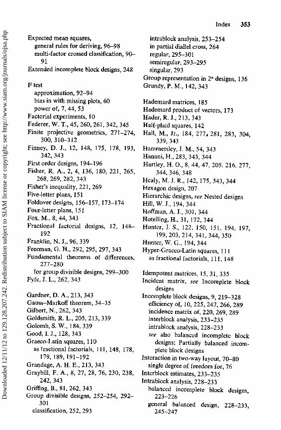
Index 353
Expected mean squares,general rules for deriving, 96-98multi-factor crossed classification, 90-
91Extended incomplete block designs, 248
F testapproximation, 92-94bias in with missing plots, 60power of, 7, 44, 53
Factorial experiments, 10Federer, W. T., 45, 260, 261, 342, 345Finite projective geometrics, 271-274,
300, 310-312Finney, D. J., 12, 148, 175, 178, 193,
342, 343First order designs, 194-196Fisher, R. A., 2, 4, 136, 180, 221, 265,
268, 269, 282, 343Fisher's inequality, 221, 269Five-letter plans, 151Foldover designs, 156-157, 173-174Four-letter plans, 151Fox, M., 8, 44, 343Fractional factorial designs, 12, 148-
192Franklin, N. J., 96, 339Freeman, G. H., 292, 295, 297, 343Fundamental theorems of differences,
277-280for group divisible designs, 299-300
Fyfe, J. L., 262, 343
Gardner, D. A., 213, 343Gauss-Markoff theorem, 34-35Gilbert, N., 262, 343Goldsmith, R. L., 205, 213, 339Golomb, S. W., 184, 339Good, I. J., 128, 343Graeco-Latin squares, 110
as fractional factorials, 111, 148, 178,179, 189, 191-192
Grandage, A. H. E., 213, 343Graybill, F. A., 8, 27, 28, 76, 230, 238,
242, 343Griffing, B., 81, 262, 343Group divisible designs, 252-254, 292-
301classification, 252, 293
intrablock analysis, 253-254in partial diallel cross, 264regular, 295-301semiregular, 293-295singular, 293
Group representation in 2n designs, 136Grundy, P. M., 142, 343
Hademard matrices, 185Hademard product of vectors, 173Hader, R. J., 213, 343Half-plaid squares, 142Hall, M., Jr., 184, 277,, 281, 283, 304,
339, 343Hammersley, J. M., 54, 343Hanani, H., 283, 343, 344Hartley, H. 0., 8, 44, 47, 205, 216, 277,
344, 346, 348Healy, M. J. R., 142, 175, 343, 344Hexagon design, 207Hierarchic designs, see Nested designsHill, W. J., 194, 344Hoffman, A. J., 301, 344Hotelling, H., 31, 172, 344Hunter, J. S., 122, 150, 151, 194, 197,
199, 203, 214, 341, 344, 350Hunter, W. G., 194, 344Hyper-Graeco-Latin squares, 111
as fractional factorials, 111, 148
Idempotent matrices, 15, 31, 335Incident matrix, see Incomplete block
designsIncomplete block designs, 9, 219-328
efficiency of, 10, 225, 247, 266, 289incidence matrix of, 220, 269, 289interblock analysis, 233-235intrablock analysis, 228-233see also balanced incomplete block
designs; Partially balanced incom-plete block designs
Interaction in two-way layout, 70-80single degree of freedom for, 76
Interblock estimates, 233-235Intrablock analysis, 228-233
balanced incomplete block designs,223-226
general balanced design, 228-233,245-247
Dow
nloa
ded
12/1
1/12
to 1
29.1
28.2
07.2
42. R
edis
trib
utio
n su
bjec
t to
SIA
M li
cens
e or
cop
yrig
ht; s
ee h
ttp://
ww
w.s
iam
.org
/jour
nals
/ojs
a.ph
p

354 Index
Intrablock analysis (continued)
group divisible designs, 253-254PBIB designs, 256-259
Intrablock subgroup, 138
James, E., 240, 344James, G. S., 28, 344John, J. A., 266, 322, 323, 326, 344John, P. W. M., 28, 139, 161, 163, 165,
167, 170, 192, 226, 246, 248, 320,344
Johnson, J. D., 321, 344
Kapadia, C. H., 259, 345Kelly, B. K., 139, 341Kempthorne, 0., 5, 8, 10, 27, 78, 81,
109, 187, 189, 230, 247, 260, 261,262, 265, 289, 322, 339, 345
Kempthorne's conjecture, 10, 247, 265,289
Keuls, M., 45, 345Kishen, K., 144, 172, 340, 345Kruskal, W. H., 46, 345
Lancaster, H. 0., 28, 31, 345Laha, R. G., 290, 347Latin rectangles, 142-143Latin squares, 105-121
experiments using several, 114-121orthogonal sets, 111-114, 221-222,
270Latin square designs, 12, 105-121
analysis of, 106-107limitations of, 108-109use as fractional factorials, 107
Lattice designs, 240, 260-262, 271, 307Least significant difference, 44, 226Legendre symbol, 185, 276Leslie, R. T., 145, 340Linear models, 18Linked block designs, 290-291, 302-
303, 312singly linked blocks, 291, 302, 312triangular doubly linked blocks, 303
Liu, C. W., 301, 309, 341Liu, W. R., 301, 305, 308, 309, 341Live factors, 160Live subscripts, 97Loraine, P. K., 139, 341Lucas, H. L., 117, 345
Madow, W. G., 33, 345Main effects, 10, 42, 67, 125Main effects clear plans, 151Main effects only designs, 151Margolin, B. H., 160, 172, 173, 174,
190, 345Marsaglia, G., 28, 343Matrices, idempotent, 15, 31, 335Measure polytope, 204Mesner, D. M., 256, 306, 312, 316, 340,
345Mikhail, W. F., 227, 345Miller, R. G., Jr., 45, 46, 346Minimal designs of resolution IV, 173Missing plot formulae, 37
Latin square designs, 121randomized complete block design, 592'n designs, 146
Mixed models, 10, 77-80Mood, A. M., 172, 346Mooney, R. W., 205, 213, 339Motorcycle racing, 222Multiple comparisons, 44-47Murty, V. N., 227, 346
Nair, K. R., 10, 223, 250, 251, 288,300, 316, 340, 346
Nandi, H. K., 283, 346National Bureau of Standards, 158,
181, 190, 346Nelder, J. A., 160, 346Nested designs, 80, 103Nested factors, 94Nested fractions, 170-172Newman, D., 45, 346Newman-Keuls test, 45Neyman, J., 105, 346Noncentral X2 distribution, 30-31
Octagonal designs, 203, 208Octahedron, 199Ogawa, J., 31, 305, 346Omitting 2n-k fractions, 161Optimal designs, 195Orthogonal arrays, 178Orthogonal blocking, 206-208Orthogonal Latin squares, sets of, 111-
114, 221-222, 270construction of, 111-114
Dow
nloa
ded
12/1
1/12
to 1
29.1
28.2
07.2
42. R
edis
trib
utio
n su
bjec
t to
SIA
M li
cens
e or
cop
yrig
ht; s
ee h
ttp://
ww
w.s
iam
.org
/jour
nals
/ojs
a.ph
p

Index 355
Orthogonal main effects plans, 184Orthogonal polynomials, 50Orthogonal response surface designs,
197Orthogonality of factors in two-way lay-
out, 68-70
Paley, R. E. A. C., 185, 346Parker, E. T., 114, 341Partial confounding, 134Partial geometry, 311Partially balanced association schemes,
250cubic, 319cyclic, 255, 315group divisible, 252, 292-301hierarchic GD, 317Latin square, 255, 305-308L.(n,m), 327LS3, 321negative Latin square, 256, 306, 312rectangular, 318T.(m), 320triangular, 254, 301-305, 320
Partially balanced incomplete block de-signs, 10, 223, 250-267, 288-328;see also the various schemes
choice of, 266combined estimates, 259intrablock analysis, 256
Patterson, H. D., 117, 346Pearson, E. S., 8, 44, 47, 216, 346Peart, J. N., 346Petersen, E. M., 346Permutation tests, 5Plackett, R. L., 27, 170, 172, 178, 184,
231, 347Plackett and Burman designs, 172, 178,
184-187,195Plaid squares, 142Polygonal designs, 201-203Pooling sums of squares, 86Power calculations, 7, 44, 53Principal block, 138Principal fraction, 149Proper designs, 227, 246Proportional frequencies, condition of,
68-70, 187Pseudo inverses, 223
Quadratic forms, 15, 17, 332distribution of, 17, 29-31independence of, 31rank of, 17
Qualitative factors, 48, 124Quantitative factors, 48, 124Quasi-Latin squares, 140, 158, 260Quenouille, M. H., 129, 347
Raese, J. T., 347Raghavarao, D., 172, 303, 306, 308,
317, 319, 347Random effects, 11, 52, 76Randomization, 4, 5Randomization tests, 5Randomized complete blocks, 9, 55-60
analysis of covariance in, 63missing plots in, 59
Rao, C. R., 23, 178, 236, 242, 245, 251,256, 269, 316, 346, 347
Rao, V. R., 246, 347Rayner, A. A., 129, 347Recovery of interblock information,
see Interblock estimatesReduced intrablock equations, 229Replication, 4, 87Residual effects, 117
designs for experiments with, 120Residuation, see Block sectionResolution of a fractional factorial, 151Resolvable designs, 226, 240, 270, 286,
299Ridge surface, 213Rising ridge, 213Response surfaces, 14, 193-213Rollingson, D. H. L., 68, 347Rotatability, 197Roy, J., 10, 247, 290, 347Roy, P. M., 227, 293, 317, 318, 347Ryser, H. J., 114, 269, 276, 277, 283,
341, 343
Saddle surface, 213Sample size, calculation of, 7Satterthwaite, F., 93, 347Saturated fractions, 155, 172Scheffé, H., 2, 5, 6, 8, 27, 35, 45, 54,
65, 78, 96, 109, 231, 348
Dow
nloa
ded
12/1
1/12
to 1
29.1
28.2
07.2
42. R
edis
trib
utio
n su
bjec
t to
SIA
M li
cens
e or
cop
yrig
ht; s
ee h
ttp://
ww
w.s
iam
.org
/jour
nals
/ojs
a.ph
p

356 Index
Scheffé's S statistic, 45, 226Schneider, A. M., 200, 348Schützenberger, M. P., 269, 348Screening experiments, 13, 149Second order designs, 196Seshadri, V., 238, 242, 343, 348Shimamoto, T., 250, 252, 256, 316, 340Shrikhande, S. S., 114, 252, 265, 269,
288, 291, 292, 295, 298, 299, 301,306, 312, 316, 323, 340, 348
Singh, K. N., 320, 327, 348Singh, N. K., 320, 327, 348Single degrees of freedom, 48-52, 73-
76Tukey's test for interaction, 76
Smith, C. A. B., 277, 348Smith, H., 21, 342Solution matrices, 24
general methods of obtaining, 26-28for reduced intrablock equations,
230-233Split plots, 11, 98, 142Split-split plots, 101Sprague, G. F., 81, 348Sprott, D. A., 245, 249, 269, 283, 284,
348Standard order, 128, 132Steel, R. G. D., 46, 348Steepest ascent, 208Steiner, J., 283, 348Stevens, W. L., 113, 348Stockett, A. L., 200, 348Studentized range, 45Student's t distribution, approximation
with unequal variances, 6Subdivision of sums of squares, 73
for 3n design, 130Sums of squares, general rules for de-
riving, 96subdivision, 73
Tanden, R. K., 101, 348Tang, P. C., 44, 348Tang's tables, 8, 44Tarry, G., 114, 349Tatum, L. A., 81, 348Three-letter plans, 151Three quarter replicates, 163
Transformations to stabilize variance,7
Triads, method of, 304Two f.i. clear plans, 151Tukey, J. W., 45, 76, 78, 342, 349Tukey's test for treatment differences,
45, 226
Unequal variances, 6Uniqueness of association schemel,
-k2 , 306triangular, 301
Vajda, S., 312, 349Vance, F. P., 182, 349Variance efficiency, 155Vartak, M. N., 318, 349
Wallis, W. A., 46, 345Webb, S. R., 173, 174, 349Webb's conjecture, 173Weeks, D. L., 238, 259, 343, 345Weighing designs, 172Weiner, S., 145Welch, B. L., 6, 93, 349Whole plots, 11, 98Widdowson, F. V., 349Wilk, M. B., 5, 78, 109, 349Williams, E. J., 120, 349Wilson, K. J., 14, 151, 193, 194, 341Wishart, J., 60, 339Wolock, F. W., 322, 342Woodman, R. M., 91, 349
Yang, C. H., 172, 349Yates, F., 2, 12, 37, 74, 98, 123, 127,
135, 141, 142, 145, 220, 233, 238,242, 260, 265, 268, 270, 282, 343,349, 350
Yates' algorithm, 127, 153checks on calculations, 128-130extension to 3n designs, 132
Youden, W. J., 122, 290, 350Youden square, 277Youle, P. V., 211, 213, 341
Zebu cattle, 68Zelen, M., 181, 293, 350Zero-sum column vectors, 185
Dow
nloa
ded
12/1
1/12
to 1
29.1
28.2
07.2
42. R
edis
trib
utio
n su
bjec
t to
SIA
M li
cens
e or
cop
yrig
ht; s
ee h
ttp://
ww
w.s
iam
.org
/jour
nals
/ojs
a.ph
p