Board of Governors of the Federal Reserve System

International Finance Discussion Papers

Number 572

November 1996

MONEY, POLITICS AND THE POST-WAR BUSINESS CYCLE

Jon Faust and John Irons

NOTE: International Finance Discussion Papers are preliminary materials circulated

to stimulate discussion and critical comment. References to International Finance

Discussion Papers (other than an acknowledgment that the writer has had access

to unpublished material) should be cleared with the author or authors.

Abstract

While macroeconometricians continue to dispute the size, timing, and even the ex-

istence of e�ects of monetary policy, political economists often �nd large e�ects of

political variables and often attribute the e�ects to manipulation of the Fed. Since

the political econometricians often use smaller information sets and less elaborate

approaches to identi�cation than do macroeconometricians, their striking results

could be the result of simultaneity and omitted variable biases. Alternatively, polit-

ical whims may provide the instrument for exogenous policy changes that has been

the Grail of the policy identi�cation literature. In this paper, we lay out and apply a

framework for distinguishing these possibilities. We �nd almost no support for the

hypothesis that political e�ects on the macroeconomy operate through monetary

policy and only weak evidence that political e�ects are signi�cant at all.

Money, politics and the post-War business cycle

1Jon Faust and John Irons

Suppose you were looking for a simple economic rule of thumb for remembering

what party held the White House in each post-War presidential term. You would

be hard pressed to do better than the following rule: if a recession starts in the �rst

6 quarters of term, its a Republican; otherwise its a Democrat. This rule calls 12 of

13 presidential terms|its one faux pas is calling Reagan's second term Democratic.

Political economists have uncovered many such striking associations between

political variables and headline measures of macroeconomic well-being such as eco-

nomic growth, unemployment, and in ation. Evaluating the size and cause of such

2e�ects has generated a ourishing literature. One leading explanation for the as-

3sociations in U.S. data seems to be the political manipulation of monetary policy.

These political results are all the more striking from the perspective of the ven-

erable and growing macroeconometric literature on the e�ects of monetary policy.

This literature continues to show little agreement on the size, timing, and even the

4existence of e�ects of monetary policy. The con ict between the political econo-

1 Faust is a sta� economist at the International Finance Division of the Board of Governors of

the Federal Reserve System. Irons is in the Economics Department at MIT. The authors thankOlivier Blanchard, Mike Gibson, Beth Ingram, Ed Leamer, Torsten Persson, Lars Svensson, the

econometrics lunch group and workshop at the Federal Reserve Board as well as seminar participants

at Duke, Indiana U., MIT, Northwestern, and North Carolina State for useful comments. Part ofthis work was completed while Faust was a visitor at the Institute for International Economic

Studies in Stockholm. Irons thanks the National Science Foundation for Financial Support. The

views in this paper are solely the responsibility of the authors and should not be interpreted asre ecting the views of the Board of Governors of the Federal Reserve System or of any other person

associated with the Federal Reserve System.2 Friedlaender, 1973; Nordhaus, 1975; Hibbs, 1977, 1987; MacRae, 1977; Frey and Schneider,

1978; McCallum, 1978; Tufte, 1978; Golden and Poterba, 1980; Beck, 1982; Browning, 1985; Allen,

1986; Chapell and Keech, 1978; Richards, 1986; Soh, 1986; Alesina and Sachs, 1988; Haynes and

Stone, 1989,1990; Bizer and Durlauf, 1990; Ellis and Thoma, 1991; Allen and McCrickard, 1991;

G�artner and Wellersho�,1991; Havrilesky and Gildea, 1991a,b; Alesina and Roubini, 1992; Alesina,

Londregan and Rosenthal, 1993; Hess, 1993; Klein, 1993; Alesina and Rosenthal, 1995; Bange,

Bernhard, and Granato, 1995.3 e.g., Alesina and Sachs, 1988; Alesina and Rosenthal, 1995.4 Recent contributions include Bernanke and Blinder, 1992; Christiano and Eichenbaum, 1992;

Leeper and Gordon, 1992, 1994; Christiano, Eichenbaum, and Evans, 1994; Hoover and Perez1994a,b; Leeper, 1993; Romer and Romer, 1989,1990,1994; Sims, 1992; Sims and Zha, 1994; Stron-

gin 1995.

metric results showing strong and consistent e�ects of politically driven monetary

policy and the less de�nitive macroeconometric results almost certainly stems from

blind spots in each approach.

The macroeocnometric literature pays elaborate attention to questions of iden-

ti�cation, attempting to sort out the e�ects of policy from among the myriad inter-

actions in a simultaneous system. Political variables are seldom if ever explored. In

contrast, virtually all of the work linking politics to economic outcomes is bi-variate,

linking one economic variable with one political variable (many such bi-variate rela-

5tions are examined). Further, the political variable|either a dummy variable for

the party in power, or some other measure of the political state|is generally treated

as exogenous, despite the fact that endogeneity of political variable is clear a priori

6and well documented. There is also a literature relating politics to instruments of

7monetary policy, rather than macroeconomic outcomes. In this literature, some

indicator of policy stance is modelled as a function of several economic and political

variables. The link from instrument to economy is generally not investigated, and

once again the political variables are often taken to be exogenous.

In light the blind spots in the literatures, we see two obvious possibilities for

resolving the con icting results. The macroeconometricians could be correct if the

political results were all due to simultaneous equations bias and omitted variable

bias. The dramatic results advanced by the political economists, however, make

it plausible that more sophisticated econometric techniques will not eliminate the

e�ects. In this case, the formal interpretation is that the political variables provide

the instrument needed for identi�cation: if the party in power determines the path

of monetary policy, and the party is itself chosen (at least in part) based on noneco-

5 Among the papers listed above, Friedlaender, 1973, is the clearest exception to the bi-variate

norm. Even when the information set includes more than one macroeconomic variable, as in G�arnter

and Wellersho�, 1991, it seldom includes the major determinants found in typical macroeconomic

models.6 Results on either side of this issue includes Stigler, 1973; Tufte, 1978; Hibbs, 1987;

Fair,1978,1982; Gleisner, 1992; Alesina, Londregan and Rosenthal, 1993; Haynes and Stone, 1994;Alesina and Rosenthal, 1995; Granato and Suzuki, undated.

7 e.g., Golden and Poterba, 1980; Beck, 1982; Allen, 1986; Richards, 1986; Allen and Mc-

Crickard,1991; Ellis and Thoma, 1991; Bange, Bernhard, and Granato, 1995.

2

nomic factors, then political variables may be the instruments for exogenous policy

changes that has been the Grail of the policy identi�cation debate.

This paper provides a theoretical econometric framework for addressing issues of

causality from politics to the economy. This framework sheds some light on strengths

and weaknesses of earlier work and provides the basis for a new look at the evidence.

While the basic approach is very general, the particular application should be viewed

as a �rst step and has several limitations. We consider only one political variable, the

party in the White House, and ignore Congressional issues raised, e.g., by Alesina,

Londregan and Rosenthal [1993]. We do not allow for systematic di�erences across

administrations of a given party, which have been found to be important in some

work [e.g., Beck, 1982]. Because we are focussing on special issues that arise under

a �xed, long election cycle, we consider only U.S. data. For the most part, we

consider only the major macroeconomic variables: output, employment, interest

rates, money, and in ation. In focussing on the links from politics to the economy,

we do not model the reaction functions as carefully as work focussing on reaction

functions exclusively. Further, we limit ourselves largely to linear e�ects. Finally,

8we consider only data since 1948.

We �nd most support for the view that political e�ects on the economy, if they

exist, are small and di�cult to measure with con�dence. Thus, omitted variable and

simultaneous equation bias appear to be a large problem in the political econometric

work �nding large and systematic e�ects. We �nd some evidence that the party in

power a�ects output growth|the party in power seems to help some in accounting

for the recession that has historically followed the election of Republicans. This

evidence is very weak and not robust to various reasonable alterations of the spec-

i�cation. We �nd almost no support for the view that any political e�ects operate

through monetary policy. Thus, the reaction of interest rates, money, and in ation

to the party in power appear economically small and statistically insigni�cant.

The results cast strong doubt on earlier results in the political econometric lit-

8 Good a priori reasoning and econometric work support the view that there is little hope of�tting a stable, linear macroeconomic model for the entire century.

3

erature that ignore the sources of bias discussed above. Because of the limitations

outlined above, these results should be interpreted cautiously. A reasonable interpre-

tation is that political e�ects are not large and systematic enough to be measured

using relatively standard methods and macroeconomic information sets. Finding

those e�ects will either require putting more structure on the problem in the form

of a priori assumptions, using more powerful statistical methods, or bringing di�er-

ent information to bear.

In section 1, we review the theories and present a preliminary look at the data.

Section 2 lays out our theoretical framework; Section 3 presents evidence from mul-

tivariate systems, and Section 4 concludes.

1 A preliminary look at the theories and data

1.1 Political business cycle theories

There is a wide range of theories about the links between politics and the economy.

Alesina and Rosenthal [1995] provide a good summary. For our purpose, a coarse

characterization will be su�cient.

The �rst important distinction is whether the theories focus on partisan di�er-

ences in the control of instruments or on behavior that should be common to the

parties. For example, Nordhaus's [1975] theory posits that either party in power

should stimulate the economy before elections to enhance its election prospects by

a myopic electorate. Partisan theories [such as Hibbs, l977] posit that the parties

should control the instruments according to di�erent objective functions, imply-

ing that the instruments and the economy should behave di�erently under the two

parties.

The second distinction is whether the stochastic nature of election outcomes is

a crucial part of the theory. Under both Nordhaus's and Hibbs's theories, the party

in power is stochastic, but this feature plays no central role in the predictions of the

theory. In contrast, in Alesina's [1987] rational partisan theory, crucial implications

turn on the e�ects of surprise changes in policy that come from election surprises.

4

In particular, the parties implement di�erent preferred average rates of in ation.

A surprise election outcome in favor of Democrats leads to a surprise increase in

in ation, which has the textbook stimulative e�ects on the economy.

From this characterization, a few gross facts are clear. We wish to have an

approach that allows us to identify systematic changes in instruments and outcomes

that vary with the deterministic election cycle. These e�ects may or may not vary

by party. We also want to have an approach that allows us to identify the e�ects of

election surprises, where these e�ects may also vary by party. Below, we derive an

econometric framework that will accommodate these desiderata.

Although our framework would allow it, we do not specify formal representations

of the theories and test them directly. Formal models must abstract from myriad

issues present in reality, and any direct test of those model must, thereby, be viewed

as a test of the joint hypotheses imbedded in the core of the formal model along with

the auxiliary simplifying assumptions. Such tests shed little light on whether the

core insights of the model are valid. Below we derive and test hypotheses associated

with core implications of models. Further work sharpening these hypotheses might

well be warranted.

1.2 A preliminary look at the real variables

We begin our examination of the data with some graphs that highlight the as-

sociations between political and economic variables and suggest pitfalls in trying

to identify political e�ects on the economy. We focus on the period 1948q1 to

1995q2, which includes thirteen presidential terms (the �rst and last terms are in-

complete). Of the thirteen terms, 7 are Republican; the parties came in the order

D D R R D D R R D R R R D. Throughout, we take no account of the fact that

Kennedy and Nixon served incomplete terms.

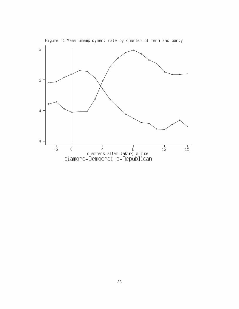
Figure 1 shows the average unemployment rate by party beginning 3 quarters

before taking o�ce through the end of the 4-year cycle. The data are averaged over

5

9the presidential terms in our sample. On entering the White House, Republicans

are greeted by an unemployment rate about one percentage point lower than are

Democrats; the rate begins to rise sharply in the third quarter in o�ce and, by the

sixth quarter, has begun to stabilize at a level that is more than a percentage point

higher than on inauguration day. The opposite pattern is shown under Democrats,

the rate falling by more than a percentage point before stabilizing.

Because averages can be dominated by outliers, we examine the median and

interquartile range of the unemployment rate under the two parties (Figure 2). For

each party, the time-series line connects the median, and the vertical bar gives the

interquartile range. The interquartile range for the Democrats is displaced slightly

to the left of the relevant quarter, while that for the Republicans is displaced to

the right. The di�erences in the unemployment rates under the two parties are

quite broad based. The median Republican shows a lower unemployment rate than

ththe 25 percentile Democrat until the cross-over point in quarter 5, after which

ththe median Republican is above the 75 percentile Democrat. In 7 of the �nal 9

thquaters of term, the 75 percentile Democrat has a lower unemployment rate than

ththe 25 percentile Republican.

As the unemployment rate moves sharply in opposite directions in quarters 3{5

under the two parties, growth in hours of employment diverges widely (Figure 3).

This widely divergent hours growth implies widely divergent output growth (Figure

104). Average output growth during quarters 3 and 4 is 5.3 percent under Democrats

and -1.6 percent under Republicans|a di�erence of about seven percentage points.

The negative growth early in Republican administrations generally marks an

NBER business cycle peak. We noted above that 6 of 7 Republicans and no

Democrats had recessions start in the �rst 6 quarters of term. Only two of 6

Democrats had recessions begin in their terms: 1948q4 came at the end of Tru-

9 Throughout, the quarters of the term are numbered from zero in the quarter of regularly

scheduled inaugurations.10 Analogous pictures show a similarly robust pattern in consumption (with a median di�erence

about half as large as for income) and investment (with a median di�erence over twice as large),

but not in government spending.

6

man's �rst term; 1980q1 began Carter's credit control recession.

1.3 Nominal variables

Republicans come into o�ce to higher interest rates than Democrats; rates fall under

Republicans as the economy slows, and rise under Democrats as it accelerates. In

the second half, the di�erences between the parties are not robust (Figure 5). Note

that this pattern in the interest rates is about what one might have expected from

looking at the real variables, without knowing that the sample has been sliced by

party. Of course, this fact would be missed in a univariate system.

The median in ation rate is higher when Republicans come into o�ce and falls

slightly over the term; the rate under Democrats rises during the term (Figure 6).

After quarter 5, however, the di�erences are not robust. While in ation is rising

steadily under Democrats in quarters 0 through 6, the M2 growth rate is falling

(Figure 7).

1.4 Implications for more formal analysis

While these results are tantalizing, they both demand careful statistical analysis

and portend complex problems for the analyst. Two facts are clear: First, indica-

tor variables for the party in power and stage in the presidential term are corre-

lated with a wide range of nominal and real economic variables. Second, economic

variables|particularly unemployment and interest rates|at the time of the elec-

tion are correlated with the subsequent election outcome. These two facts can be

summed up in the claim that there is a rich simultaneity with both rich lead and

lag relations among the macroeconomic and political variables.

This rich simultaneity suggests that omitted variable bias and simultaneous equa-

tions bias will be major concerns in any work relating endogenous political variables

to macroeconomic variables. While the association between party in power and the

unemployment rate might be due to political manipulation of policy, it might just

as well be due to causality from the economy to the party in power. Suppose the

7

electorate chooses a Republican to run the country when the unemployment rate is

below the natural rate and Democrats when it is above. If the unemployment rate is

stationary, below average unemployment rates are naturally followed by rising rates.

This might account for Figure 1 without relying on any causality from politics to the

economy. On the other hand, if this reverse causation from economy to politics is to

account for Figure 1, it must be the case that, in e�ect, the electorate can forecast

one percentage point rises in the unemployment rate about a year in advance with

great accuracy. Otherwise, they could not reliably put Republicans in o�ce when

such a rise is coming. It is not clear that unemployment rate rises are su�ciently

predictable.

A somewhat richer illustration of problems measuring political e�ects comes from

recent empirical work by Alesina and Rosenthal [1995] explaining in ation in terms

of its own past and the party in power. In support of the claim that Democrats

implement higher rates of in ation than Republicans, Alesina and Rosenthal cite

the following regression:

I = 1:2 + 1:3 I � 0:3 I + 0:1 It t�1 t�2 t�3

(5:4) (17:4) (�2:9) (0:7)

� 0:2 I � 0:6 BW� 0:3 Repub + 0:7 oilt�4 t�3 t

(�2:4) (�4) (�2:5) (2:9)

(We produced these results, which very nearly replicate those of Alesina and Rosen-

thal.) In this regression, I is annual CPI in ation, BW is a dummy variable that

is one under the Bretton Woods system (through 1971) and zero otherwise, Repub

is a variable that is one under Republicans and zero otherwise, and oil is a dummy

variable that is one during 1973q3-1974q4 and 1979q4{1980q4. The sample period is

1949q1{1991q4; t-statistics are under the coe�cients. Alesina and Rosenthal inter-

pret the coe�cient on Repub as evidence that Republicans implement lower in ation

rates than Democrats, and that the e�ect begins to operate after three quarters in

o�ce.

Since the Repub dummy is endogenous we might worry that it is standing in

for other macroeconomic variables that are important in determining in ation. For

8

example, if the evolution of in ation depends on labor market tightness, as it does

in a wide range of theoretical models, then Figures 1 and 2 suggest that the Repub

dummy may enter this regression signi�cantly acting as a crude proxy for current

11and past labor market tightness. If we suspect that the Repub dummy is a proxy

thfor economic variables then we might expect 16 order serial correlation in this

regression|the macro variables move smoothly, but the dummy is constant for 16

thquarters at a time. The LM test for absence of 16 order serial correlation rejects

at less than the 0.01 percent level. We add enough lags of in ation to eliminate

the symptoms of serial correlation (13 lags) and include one lag of growth in hours

to allow for an association between labor market tightness and in ation. In this

regression, hours enters the regression very signi�cantly (coe�cient 0.04, t-statistic

3.8) and the e�ect of the political dummy falls to one-sixth its previous magnitude

and becomes statistically insigni�cant (coe�cient -0.05, t-statistic -0.7).

We present this brief result not because this is our preferred in ation equation,

but to illustrate a general and important point:

Due to simultaneous equations and omitted variable bias, there is little

a priori reason to expect robustness of political business cycle results

that are based on a small macroeconomic information set and that treat

political variables as exogenous.

In the following section, we lay out a framework for dealing with these problems.

2 Speci�cation and identi�cation of a simultaneous system of macroe-

conomic and presidential cycle variables

The political variable considered here provides some special opportunities and spe-

cial problems, each of which stem from the fact that the party in power takes on only

two values and changes only every 16 quarters. The framework we adopt is quite

general, but the particular implementation we choose is designed to be the simplest

11 Note that using lagged values as instruments might solve the simultaneity problem (if theinstruments are valid), but will not solve the problem stemming from omitting serially correlated

variables.

9

possible generalization of the identi�ed vector autoregression (VAR) approach. We

choose this implementation because it provides both a simple and a natural start-

ing point given the current prominence of VAR work for identifying the e�ects of

monetary policy.

2.1 Deriving and identifying the standard VAR

Take one political variable z and an (n� 1) vector of macroeconomic variables X ,t t

and posit that these variables are determined by

2 3zt6 7 ~= f (~z ; X ; e ) (1)4 5 t�1 t�1 t

Xt

0 0 0 0~where X = (X ;X ; : : : ;X ) , ~z is similarly de�ned, and e is a vector of ex-t t tt t�1 t�p

ogenous shocks. For any plausible macroeconomic model, f is nonlinear, but we

12typically take a linear approximation to the model to give

2 3 2 3z ~zt t�16 7 6 7

= �+B + " (2)4 5 4 5 t

~X Xt t�1

Equation (2) is a vector autoregression (VAR) and is often written,

2 3zt6 7

B(L) = � + " (3)4 5 t

Xt

where Lz = z and B(L) is a matrix polynomial in L. The nonlinear modelt t�1

is (generically) identi�ed [McManus, 1992], but in linearizing we take on an iden-

ti�cation problem arising from the fact that (3) is observationally equivalent to

0 0 � �C(L)[z ;X ] = c + " where C(L) = CB(L), c = C� and " = C" , and C is fullt tt t t

rank. Each such C gives a di�erent identi�cation of the system, and the response

of the economy to a shock, say, in the political variable is di�erent in each.

12 We attempt to choose the approximation and some transform of the variables so that " hast

constant mean and variance, and is serially uncorrelated. The adequacy of the linear approximationis testable, and the evidence for nonlinearities in U.S. macroeconomic data has not been strong

enough to justify abandoning the linear framework.

10

In this paper, we only attempt to identify the e�ects on X of an exogenous shiftt

in the z equation. Thus, we only identify the e�ects of an election shock. If wet

ignore the special properties of the z variable, two assumptions will be su�cient fort

identi�cation. First, assume that in each quarter, the value of the political variable

z is determined before any other variable. This suggests a block recursive structuret

of the economy as in Sims [1980a], in which X does not enter the z equationt t

contemporaneously. Second, assume that " is orthogonal to all the other "s at all1t

leads and lags. That is, we place z �rst in a block recursive ordering of the VARt

and assume that " is orthogonal to the remaining " at t.1t jt

Under these assumptions, we can estimate the model and calculate the dynamic

e�ects of a one-period exogenous shift in the z equation. The dynamic e�ects oft

thsuch a change on the j X variable are summarized in an impulse response function,

which is the sequence of numbers,

a = �@X =@" i = 0; 1; : : : (4)ji jt+i 1t

13where � is an arbitrary scaling re ecting the size of the presumed exogenous shift.

The scheme laid out in the following section is the natural generalization of this

scheme to allow for the special nature of z .t

2.2 Taking account of the presidential cycle variable

Our z is an indicator for party in power and is equal to 1 if a Democrat is int

the White House at t and is zero otherwise. Thus, z is discrete and changes onlyt

every 16 periods in quarterly data. To deal with these special features, de�ne

q(t) 2 f0; : : : ; 15g as the time t quarter of the presidential term, numbering from

zero. Now assume that z evolves according to:t

13 thThe coe�cient a (up to a proportionality factor) is given by (1; j) element of the matrixjiP1 m �1A , where A(L) = A L and A(L) = B(L) .i mm=0

11

i) E z = z for all t; q(t);t�1 t t

ii) z = z if q(t) 6= 0, andt t�1

~iii) E [z ] = �(X ; z ) if q(t) = 0:t�2 t t�2 t�2

Thus, the party in power may change every 16 quarters; it is picked based on the

economy 2 quarters earlier; and the outcome of the election is known one quar-

ter before the president takes power. Further, the probability that a Democrat

will win, based on the macroeconomic variables and the current party in power, is

~�(X ; z ). These assumptions would be exactly appropriate if the election weret�2 t�2

held October 1 and the president took power January 1. We will model as if this

slightly modi�ed timing were correct.

Now replace the general representation of the economy in (1) with,

8>< z if q(t) 6= 0t�1z = (5)t > ~: �(X ; z ) + u otherwiset�2 t�2 t�1

�~X = G(q(t); z ; z ;X ; � )t t+1 t t�1 t

In G, we allow the presidential party this quarter and next quarter to a�ect this

quarter's economy. Of course, both of these values are always known, and the two

14can only di�er in the �nal quarter of term. Why is q(t) an argument of G? It

will obviously be relevant under Nordhaus-style theories. It may also be relevant

under rational partisan theories since political uncertainty is not homoskedastic

through time. Macro variables will fail to be homoskedastic if political uncertainty

has important e�ects on the economy.

Of course, some form of time homogeneity must be imposed. Notice that

(z ; z ; q(t)) form a triplet of discrete variables. It is natural to view this triplett+1 t

as the state of the political economy at t and to assume that the economy is homo-

geneous conditional on the political state. Call the set of the 34 possible values of

14 Further, lags of z could be included without changing the analysis.t

12

15this state variable . We can re-write the X equation as

�~X = G (X ; � )t t�1s(t) t

where s(t) 2 is the political state at t. The evolution of the state variable is

governed by (5) and the exogenous quarter-of-term variable. After linearizing, the

analog of the macroeconomic VAR in (2) is now

~X = � + B X + �t t�1 ts(t) s(t)

This expression says that the VAR representation for X has di�erent � and Bt

coe�cients depending on the value of the political state. One can also write system

as,X X

~X = � d + B d X + � (6)t ! !;t ! !;t t�1 t

!2 !2

where d = 1 if ! = s(t) 2 and d is zero otherwise. Thus, d is an indicator!;t !;t !;t

that is one if the state at t is ! and zero otherwise. Equation (6) says that we simply

need to take the standard macroeconomic VAR and augment it with political state

dummy variables interacted with the intercept and with all the slope coe�cients.

These dummy variables are not exogenous, but since their values at t are known

at t� 1, they are predetermined. Of course, the system still involves the nonlinear

equation for z . We show below that we can do the inference we wish to do simplyt

by estimating the augmented VAR and need not estimate the nonlinear part of the

model.

The form of the augmented VAR is similar to the model estimated by Ellis

and Thoma [1991]. Ellis and Thoma derived no structural interpretation on the

form, however, and considered a very limited speci�cation, and, hence, face the

16identi�cation and omitted variable problems common in the rest of the literature.

15 For the �rst 15 quarters of the term z = z and can take on two values; in the �nal quarter,t t+1

there are four possible values.16 More speci�cally, Ellis and Thoma treated the d variables as exogenous; they examined impulse

responses derived from an arbitrary recursive ordering of the VAR attributing nothing to the shock

in the d variables. Their VAR included instruments of policy, but no macroeconomic variables that

may be important in determining those instruments.

13

It is clearly impossible to estimate the coe�cients of (6) in the post-War macro

data. The summation over involves 34 possible values of the state variable. Thus,

the political model involves 34 times the (already large) number of coe�cients in a

standard macroeconomic VAR. This parsimony problem is similar to the one faced

in most macro applications, and we deal with it in a standard manner as outlined

below.

2.3 Hypotheses of interest

The sketch of political theories above suggests three nested hypotheses regarding

the augmented VAR model. At the coarsest level, we are interested in whether any

political variables need to be included in macroeconomic models. In the augmented

VAR this is a matter of whether coe�cients can be constrained to be constant across

the political state, s(t). Thus, the hypothesis that the political state is irrelevant is:

H : � = � and B = B for all m;n 2 0 m n m n

IfH does not hold, we can consider the Nordhaus theory in which economic activity0

may vary with quarter of term but not with the value of the party in power. De�ning

Q(m) as the quarter of term in state m, the hypothesis is

H : � = � and B = B whenever Q(m) = Q(n)1 m n m n

Under H , we �nd quarter-of-term e�ects, but no partisan di�erences. Rejection of1

H and H is evidence of partisan e�ects:0 1

H : � 6= � or B 6= B for some m; n with Q(m) = Q(n)2 m n m n

Sorting out whether these e�ects are due to surprise e�ects, as in the rational par-

tisan theory, or due to di�erences in policy that do not have their e�ects through

surprises does not involve simple restrictions on the coe�cients. We can, however,

look at the impulse response to election shocks to see if the pattern favors a partic-

17ular interpretation.

17 Even stronger evidence would come from seeing e�ects that di�er with the degree of electionsurprise. Since we do not estimate the z equation, we cannot pursue this angle here.

14

2.4 Identi�cation in the augmented model

Before we can test the hypotheses above, we must be able to form estimates that are

arguably free from simultaneity bias. We now have a model comprised by a nonlinear

model for z , which determines the d variables, and (6), an augmented VAR. Ast m;t

in the discussion of the standard case outlined above, we rely on a block recursive

structure of z and X and an orthogonality assumption. Under the assumed timingt t

of events, z belongs �rst in a causal ordering of the model. We must also assumet

that the election shock u is uncorrelated with � for all s; t. Economically, thist s

amounts to the decision to attribute to the political variable any macroeconomic

outcome that is correlated with the election surprise. This assumption would be

~inappropriate if variables other than X that determine the outcome of the electiont

at the end of period t also directly a�ect the economy. Suppose, for example, that

news arrives in the third quarter of an election year of the breakdown in some peace

talks. The breakdown might well alter the re-election prospects of the president

18and also directly a�ect the economy through its e�ects on military procurements.

While it is easy to come up with examples like this, it is more di�cult to come up

with such examples that systematically favor one party or the other, thus inducing

a spurious correlation between party and economy. By considering a large range of

economic variables, and by considering the sensitivity of the results to changes in

the information set, we hope to minimize this risk.

Validity of these assumptions is su�cient to allow us to estimate consistently

the augmented VAR for X while including z and z (through the d variables) int t t+1

the equations. The �nal issues concerns calculating the response of macro variables

to the election shock.

18 Faust and Leeper [1993], building on Hansen and Sargent [1991b] and Marcet [1991], question

assumptions about the correlation of structural shocks based on problems with time-aggregated

data. Given the nature of the z variable, these problems would not exist here if the election weret

in fact held on Oct. 1, and we believe that these e�ects will be small in practice.

15

2.5 The impulse response to election shocks

Because the z equation is nonlinear, several complications arise regarding what wet

mean by an impulse response function [see, e.g., Gallant, et al., 1993]. Several of

these are simpli�ed by limiting ourselves to a 16 quarter impulse response, starting

in quarter 15 of a presidential term, which we also call quarter -1 of the following

term. Election shocks happen only at the beginning of quarter -1, implying that the

process for z and z (and, hence, for the d variables) is conditionally determinis-t t+1 t

tic for quarters 0 through 14 of the term. The next shock happens at the beginning

of quarter 15 (=-1). Thus, the 16 quarter impulse response of the political state to

an election shock at quarter -1 is trivial and depends on no unknown parameters.

Because no variables feed back on the z equation for 16 quarters, we can also com-t

pute the 16 quarter impulse response of X to an election shock without estimatingt

the nonlinear z equation.t

What we report below for the impulse response of X to an election shock atjt+i

the beginning of time t is the sequence of numbers,

@E Xt�1 jt+ia = 0:10 i = 0; 1; : : : ; 15: (7)ji

@E ut�1 t

where u is the exogenous shock to the election outcome. Note that a rise in E ut t�1 t

by 1 percentage point equals a 1 percentage point change in the probability that

a Democrat will be elected. Thus, while the standard impulse response gives the

response of X to a one standard deviation change in some shock, the modi�edj

impulse response gives the response of X to a 10 percentage point change in thej

19public's subjective probability that a Democrat will take the White House at t+1.

The impulse response is easily calculated (see the Appendix).

19 Much of the nonlinearity of the problem has disappeared in this formulation. It remains in

the z equation, however. Thus, given the history up through t � 1, only one of two shocks u cant t

happen: �� or 1��. In order to estimate the actual shocks that could have happened a t� 1, we

must estimate the z equation. Further, there is no simple notion of variance decomposition in thist

setting.

16

3 Application: A multivariate model with political e�ects

In this section, we estimate the augmented VAR. Our goals are to assess the impor-

tance of political variables in traditional macro models and to assess the role of the

monetary policy channel in accounting for any political e�ects. Thus, we begin with

a much studied VAR including four macroeconomic variables: three-month Treasury

bill rate, M2, the CPI, and GNP. These variables will be referred to as R, M, P, and

Y respectively. The RMPY system is a natural starting point. Some version of these

variables is at the core of the Friedman and Schwartz [1963] analysis and variations

of this basic VAR have been investigated extensively in assessing monetary policy

e�ects [e.g., Sims 1980b, Sims 1994].

The baseline VAR for RMPY has all variables in levels and all variables except

the interest rate in logarithms. The VAR includes a constant and three seasonal

dummies. The theoretical framework suggests that we augment the standard VAR

with slope and intercept dummies for each quarter of the term under each party. This

model is too pro igately parameterized to be of interest and is even too general to be

the starting point of a Hendry-style general-to-speci�c model search [Hendry, 1995].

Instead we start with a fairly general model, from which we derive a parsimonious

baseline model. After demonstrating the baseline results, we consider a number of

changes to the baseline model in order to assess robustness.

The estimation period is 1953q2 to 1995q2, and the lag length of six for the

macro variables was selected by serial correlation tests. For our starting point we

considered only political intercept dummies. From the possible 34 dummies for

th ththe -1 through 15 quarters of term under each party, only a subset are linearly

independent given the constant and seasonal dummies. We began with a maximal

set of these dummies, which were not jointly signi�cant at the 10 percent level,

and very few of the individual coe�cients were signi�cant at the 10 percent level.

Because of the large number of dummy variables in this regression, the test probably

has low power to reject the hypothesis of no e�ects. Thus, we tried replacing the

quarter-of-term variables for one of the parties at a time with year-of-term dummies.

17

Using Republican year-of-term variables, the the political variables were not jointly

signi�cant. Using Democratic year-of-term variables, all the of year-of-term variables

and most of the Republican quarter-of-term variables were signi�cant at the 1 or 5

percent level. We took this as our baseline model.

Thus, the baseline augmented VAR includes in four intercept dummies, dy1

through dy , that are zero except in the subscripted year of a Democratic adminis-4

tration; 15 dummies, rq ; : : : ; rq , that are zero except in the subscripted quarter of0 14

Republican administrations; and dq and rq which are zero except in the quarter�1 �1

before a Democrat or Republican take o�ce, respectively.

The model passes serial correlation tests (for �rst, fourth, and sixteenth order

correlation) and heteroskedasticity tests (Table 1, column i). Given the minimal

attempt to datamine for the best set of political variables, we take the baseline results

as relatively strong statistical evidence against H |the irrelevance of politics|in0

this model. Five of the 16 Republican dummies are signi�cant at the 1 percent level;

an additional seven are signi�cant at the 5 percent level. The political variables are

jointly signi�cant at the 7 percent level. The test of H , the absence of partisan1

e�ects, rejects at the 3 percent level.

As the point estimates of dummy variables are almost impossible to interpret in

a dynamic system, we turn now to the impulse response functions, which provide a

much more interpretable picture of the economic signi�cance of the political e�ects

(Figure 8). The point estimate of the impulse response is indicated by the circle; and

the lines are empirical 95 percent coverage intervals calculated using the Sims-Zha

20[1994] Bayesian bootstrap.

The 10 percentage point rise in Democratic election prospects generates a rise

of over half a percentage point in output growth over the �rst year in o�ce, which

dissipates by the end of the second year. This seems like a large e�ect, say, of electing

a Democrat when the ex ante probability of doing so was 90 percent. The expected

20 The procedure was implemented in Gauss by the authors. The procedure uses an ignorance

prior described by Sims and Zha. As Sims and Zha note, there is currently no entirely satisfactory

way to calculate classical con�dence intervals on impulse responses.

18

version i ii iii

variable

rq *�1

rq ** **0

rq *** ** *1

rq *** *2

rq * ***3

rq *** *** **4

rq *** **5

rq ** **6

rq ** **7

rq **8

rq *** * **9

rq *** **10

rq **11

rq *12

rq *** **13

rq **14

dq�1

dy **1

dy **2

dy **3

dy ***4

BW **

z �BW ***t

D1980q2 *** ***

D1980q3

D1980q4 *** ***

AR(1{16) ** ***

Hetero

Notes: ***, **, *, indicate signi�cance at the 1, 5, and 10 percent levels, respectively.

The signi�cance tests are F tests for inclusion of all terms involving the variable in

the model. The AR test reported is the standard LM test. The heteroskedasticity

test essentially involves a regression of the squared errors from the model on the

levels and squares of all the variables and provides a test of signi�cance of the

variables in this second stage regression. The signi�cance levels are all for the F

form of the statistic. Tests were reported by PC-FIML and are further explained in

Doornik and Hendry [1994].

Table 1: Signi�cance of political state variables in the baseline model

19

3-month Treasury bill rate follows the pattern that might be expected if the output

e�ect were due to a persistent surprise rise in money growth: interest rates fall for at

least a year and then rise by a similar amount and stay higher. The e�ect, however,

is quite small, less than 25 basis points in each direction. M2 growth shows only a

small and brief rise, and in ation shows similarly small e�ects and no economically

signi�cant pattern at all. Thus, while the basic pattern of interest rates is roughly

consistent with the election shock generating a monetary policy surprise, the e�ects

on output are probably larger than one would expect for such a small change in

interest rates, and money growth and in ation are not very supportive of the story.

These results are much less supportive of the partisan model operating through

money supply shocks than those of Alesina and Sachs [1988] and Alesina and Rosen-

thal [1995]. Those results involved interpreting political dummy variables from

univariate regressions directly without resolving the dynamic interactions among

variables or attempting to isolate the surprise element that is central to the theory.

Taken at face value, the results present a puzzle. Figures 1 through 9 and Table 1

show evidence of strong e�ects of party on aggregate measures of economic activity.

The channels through which policy causes these e�ects, however, are not clear from

any of these sources of information. One possibility is that the e�ects operate

through �scal policy. This possibility seems unlikely to account for the recession

that quickly follows Republican elections, since �scal policy is slow to change. In

any case, we investigate this channel in a separate paper [Faust and Irons, 1996],

�nding no clear evidence that �scal policy accounts for the observed output e�ects.

An alternative possibility is that the political variables are proxying for some

other source of variation in output. If this is the case, we might expect the results

to change when the speci�cation of the model is altered. Thus, we turn to the

robustness of the baseline results. We investigate 5 basic VARs: 1) the baseline

model, 2) substitute M1 for M2 in the baseline, 3) add log of hours of work to the

baseline, 4) add the log of the producer price index for intermediate materials to the

20

21baseline, 5) add the producer price index for sensitive materials to the baseline.

Model 2 is warranted because results are often sensitive to which monetary aggregate

is chosen. Model 3 is suggested by the e�ect of hours growth in the Alesina Rosenthal

regression. Models 4 and 5 are motivated by work [e.g., Sims, 1992, Sims and Zha,

1994] arguing that commodity prices can substantially alter the results from RMPY-

type VARs.

Three versions of each of the 5 models are run. Version i involves no economic

dummy variables. Version ii is motivated by the fact that in the baseline model,

1980q2 is a large outlier. This is the quarter in which credit controls were enacted

22leading to the sharpest, shortest recession in U.S. history. It is clear that we cannot

model the process leading to the imposition of credit controls, and it is important

to investigate the sensitivity of the results to this episode. Thus, version ii adds

separate dummies, labelled D1980q2 through D1980q4, for the �nal three quarters

of 1980. Version iii includes the credit control dummies and a dummy variable,

BW, that is one up until 1972. Alesina and Rosenthal use this variable because the

Bretton Woods system may have constrained in ation behavior before 1972. Many

other important changes in the macroeconomy occurred at about this time: the

onset of oil shocks and the productivity slowdown are two of the most important.

To allow for the possibility that the parties had di�erent mean in ation rates in the

post-Bretton Woods system, but the same rate in under Bretton Woods, we also

include the BW dummy interacted with the z dummy.t

The importance of these dummy variables is clear from their e�ects on the sig-

ni�cance of the political variables in the baseline model (Table 1, columns ii and

iii). For example, in versions ii and iii, none of the Democrat variables is signi�cant

at the 10 percent level and only one of the Republican variables is signi�cant at the

21 We also tried a variety of other models. We interacted all of the slope coe�cients in the model

with the z dummy. Only two of the 24 slope dummies made a signi�cant contribution to thet

system at the �ve percent level. Various other con�gurations of slope dummies were also tried with

no clear support for their inclusion. We also considered a variable measuring the relative price of oil

and the Alesina-Rosenthal oil shock dummy described above. Neither of these added signi�cantly

to the explanatory power of the model.22 This quarter involved the largest quarterly drop in R and Y in the sample. See the 1981

Economic Report of the President for an account of this period.

21

1 percent level.

Table 2 summarizes the statistical evidence for important political e�ects in the

2315 models. The Democratic and Republican political variables|the same political

variables as in Table 1|are statistically signi�cant at the 10 percent level or less

in only about 1/3 of the models (rows labelled H ). In version ii (all models) and0

model 3 (all versions), the political e�ects are never signi�cant.

We suspect that the political e�ects may still be overparameterized in this model,

and that in particular, the only important political e�ects come in the �rst half of

Republican administrations. The rows labelled H test the hypothesis that the allX

the Democratic variables and the Republican variables for quarter 9 and beyond are

zero. This hypothesis is only rejected once at the 10 percent level. Thus, it appears

that Democratic presidential terms and the second half of Republican terms are

similar and that the evidence of political e�ects comes from the recessions that

coincide with the election of Republicans.

After removing the political variables for all but quarters -1 through 8 for Re-

publicans, we can test whether the remaining Republican e�ects are signi�cant.

This is a test of both H and H , since any e�ect that is found involves a partisan0 1

di�erence. We label this hypothesis H . After limiting the set of included political0;1

dummies based on prior tests, the remaining political dummies for Republican for

quarters -1 through 8 are jointly signi�cant at the 10 percent level or better in 10

of 15 models. Of course, since we have tailored the set of variables to maximize the

measured e�ects, we should make our standards more stringent. In only 2 cases are

the dummies signi�cant at the 1 percent level. The �rst half Republican e�ects are

also insigni�cant in all versions of model 3 (involving hours). Thus, even after tai-

loring the set of dummy variables, the evidence in favor of political e�ects is mixed,

at best.

A more economically interpretable view of the VARs is given in Table 3, which

summarizes impulse response functions for the 15 models. For each model and

23 In all of the models that include economic dummies, the test of the joint hypothesis that all

the economic dummies are zero rejects at less than the 1 percent level.

22

model

hypothesis 1 2 3 4 5

i : No economic dummies

H 0.07 0.30 0.26 0.11 0.040

H 0.04 0.09 0.12 0.01 0.070;1

H 0.35 0.70 0.55 0.66 0.15X

ii : Credit Control

H 0.20 0.41 0.39 0.25 0.120

H 0.05 0.12 0.20 0.03 0.130;1

H 0.63 0.79 0.63 0.82 0.28X

iii : Credit Control & Bretton Woods

H 0.04 0.18 0.22 0.05 0.010

H 0.03 0.04 0.16 0.01 0.050;1

H 0.24 0.70 0.43 0.58 0.04X

Notes: H : all political dummies are jointly signi�cant. H : after imposing H ,0 0;1 X

all remaining political dummies (rq ; : : : ; rq ) are zero. H : all political dummies�1 8 X

except rq ; : : : ; rq are zero. The numbers reported are marginal signi�cance levels,�1 8

the tests are as described in the notes to Table 1. , , , indicate signi�cance at

the 1, 5, and 10 percent levels, respectively.

Table 2: Signi�cance of political state variables 5 models

23

version, the Table gives the averaged impulse response of Y, R, M, and P to an

election shock over the �rst and second halves of the presidential term. If signi�cant

output e�ects operate through monetary policy, we would expect to see positive

output growth e�ects in the �rst half, positive money and in ation e�ects in both

halves, and perhaps negative then positive interest rate e�ects.

In model 3, the e�ects are statistically insigni�cant and the point estimates are

24not consistent with the rational partisan story. The �rst-half output e�ects are

smaller than the second-half e�ects which may be positive or negative, depending

on the verison. The money growth e�ects are negative, and the in ation e�ects are

also negative in two versions. Only the interest rate e�ect is as expected.

The �rst half output e�ects are largest and most statistically signi�cant in ver-

sions i and iii. In these versions, however, the interest rate and money growth

e�ects are quite small, relative to the output e�ects. Further, the in ation e�ects

are small, with point estimates that are often negative. Thus, while versions i or

iii may support important �rst-half output e�ects, they provide no support for the

view that these e�ects operate through monetary policy.

The pattern of point estimates in version ii (especially model 1) is probably most

supportive of the rational partisan theory. The second-half interest rate and in ation

e�ects are in the right direction and the �rst-half output e�ects are generally large.

The money growth e�ects tend to be negative in the second-half, however.

Overall, the point estimates in Table 3 and the statistical signi�cance �gures in

Table 2 show no consistent pattern of support for important output e�ects or for

output e�ects caused by surprise changes in monetary policy.

4 Discussion

This paper highlights several questions regarding standard macroeconometric and

political econometric results and sheds some light on the answers to those questions.

24 In Table 3, the measure of statistical signi�cance comes from the Bayesian bootstrapped

coverage intervals, and not F tests.

24

model 1 2 3 4 5

variable half average response

i: No economic dummies

Output growth 1 0.24 0.18 0.10 0.18 0.18

2 0.04 0.08 0.10 0.06 0.06

3-Month T-Bill 1 -0.08 -0.12 -0.14 -0.14 -0.16

2 0.16 0.06 0.06 0.06 0.08

Money growth 1 0.10 -0.10 0.00 -0.06 -0.04

2 0.08 0.04 -0.08 0.02 -0.04

CPI in ation 1 -0.06 -0.10 -0.10 -0.12 -0.16

2 0.06 0.00 -0.06 0.00 0.06

ii : Credit Control

Output growth 1 0.16 0.12 0.00 0.12 0.16

2 -0.10 0.00 -0.06 -0.06 -0.04

3-Month T-Bill 1 0.04 0.00 -0.02 -0.02 -0.04

2 0.40 0.28 0.30 0.26 0.42

Money growth 1 0.00 -0.28 -0.16 -0.16 -0.24

2 0.16 -0.02 -0.12 0.06 -0.22

CPI in ation 1 0.20 0.14 0.18 0.08 0.10

2 0.40 0.34 0.32 0.28 0.46

iii : Credit Control & Bretton Woods

Output growth 1 0.22 0.16 0.08 0.16 0.16

2 0.08 0.12 0.16 0.12 0.12

3-Month T-Bill 1 -0.04 -0.08 -0.10 -0.10 -0.12

2 0.16 0.06 0.04 0.06 0.10

Money growth 1 0.08 -0.16 -0.06 -0.10 -0.10

2 0.12 0.10 -0.04 0.08 -0.02

CPI in ation 1 -0.02 -0.06 -0.08 -0.10 -0.14

2 0.04 -0.02 -0.10 -0.04 0.04

Notes: Half 1 is quaters -1 through 8; half 2 is quarters 9 through 15. The impulse

response is averaged over the relevant half. The symbols are as in Table 2. In this

table, a quantity is signi�cantly di�erent from zero at, say, the 10 percent level ifth ththe interval between the 5 and 95 percential points from the Bayesian bootstrap

(described in the text) does not cover zero.

Table 3: Summary of impulse response to election shock

25

On the negative side, it is clear that correlations among political variables and a

wide range of macroeconomic variables at both leads and lags renders unreliable

results from univariate work treating political variables as exogenous. We provide a

framework for sorting out these interactions.

Applying this framework, we conclude that there is some weak and fragile evi-

dence in favor of important political e�ects. The strongest evidence seems to come

from the �rst half of Republican administrations: recessions have followed the elec-

tion of Republicans and macroeconomic factors alone may not account for this fact.

There is little evidence, however, that the causal explanation of any political e�ects

on the economy operates through surprise changes in monetary policy.

These results should be viewed as a challenge to those who believe that we have

clear evidence of political e�ects, but not proof that there are no such e�ects. A

balanced conclusion is that the political e�ects are not large and systematic enough

to be easily and precisely measured. Finding such e�ects will either require putting

more structure on the problem in the form of a priori assumptions, using more

powerful statistical methods, or bringing di�erent information to bear.

26

Appendix

The method for calculating the impulse response can be seen from the augmented

VAR. The expected path of the economy at the end of t� 1 can be written,

E X = E [X jz = 1]E [z ] +t�1 jt+i t�1 jt+i t+1 t�1 t+1

E [X jz = 0](1� E [z ])t�1 jt+i t+1 t�1 t+1

Since @E [z ]=@E u = 1,t�1 t+1 t�1 t

@E Xt�1 jt+i= E [X jz = 1]� E [X jz = 0] (8)t�1 jt+i t+1 t�1 jt+i t+1

@E ut�1 t

which is simply the di�erence in the expected path of the economy under the two

parties. For i < 15, this expression can be evaluated simply from the augmented

VAR and does not depend on � or the z equation.t

Expression (8) is easy to evaluate. Similar to the calculation of impulse responses

in a standard VAR, the impulse response to election shocks can be calculated as the

di�erence in a dynamic simulation of the model under the two possible outcomes

for the election.

Data

All economic data (except M1 and M2 for the period before 1959) are from the

Federal Reserve's U.S. database. All growth rates are computed as the annualized

quarterly change in the logarithm of the variable. The data series are GNP, personal

consumption expenditures, gross private domestic investment, and federal govern-

ment purchases of goods and services from the GNP accounts, all in 1987 dollars.

The unemployment rate is for civilian males 20 years or older; hours are for all

persons in the nonfarm business sector. M1 and M2 are not seasonally adjusted;

the pre-1959 data were constructed by Robert Rasche. The Three-month T-Bill

rate is a yield from the secondary market. The in ation rate is for the CPI, all

urban consumers. The two commodity price indices are the producer price index

for intermediate materials and sensitive materials. All of the dummy variables were

constructed by the author. All data are available on request.

27

References

Alesina, A., 1987. Macroeconomic policy in a two-party system as a repeated game,

Quarterly Journal of Economics, 102, 651{678.

Alesina, A., 1991. Evaluating Rational Partisan Business Cycle Theory: A Re-

sponse. Economics and Politics, 3, 63{71.

Alesina, A. and N. Roubini, 1992. Political Cycles in OECD Economies. Review

of Economic Studies, 59, 663{688.

Alesina, A. and H. Rosenthal, 1995. Partisan politics, divided government and the

economy, Cambridge University Press: New York.

Alesina, A., J. Londregan and H. Rosenthal, l993. A Model of the Political Econ-

omy of the United States. American Political Science Review, 87 (1), 12-33.

Alesina, A., and J. Sachs, 1987. Political Parties and the Business Cycle in the

United States, 1948-1984. Journal of Money, Credit, and Banking, 20, 63{82.

Allen, S., 1986. The Federal Reserve and the Electoral Cycle. Journal of Money,

Credit, and Banking, 18, 88{94.

Allen, S. and D. McCrickard, l991. The In uence of Elections on Federal Reserve

Behavior, Economics Letters, 37, 51{55.

Bange, M., W. Bernhard, and J. Granato, 1995. Partisan Monetary Policy, In a-

tion, and Economic Growth. Michigan States University's Institute for Public

Policy and Social Research Working Paper 95-04.

Beck, N., 1982. Presidential In uence on the Federal Reserve in the 1970s. Amer-

ican Journal of Political Science, 26, 415{445.

Beck, N., 1982. Parties, Administrations, and American Macroeconomic Out-

comes. The American Political Science Review, 76, 83{93.

Bernanke, B. and A. Blinder, l992. The Federal Funds Rate and the Channels of

Monetary Transmission. American Economic Review, 82, September, 681-21.

Bizer, D., and S. Durlauf, 1990. Testing the positive theory of government �nance.

Journal of Monetary Economics, 26, 123{141.

Browning, R., l985. Presidents, Congress, and Policy Outcomes: US Social Welfare

Expenditures, l949-77. American Journal of Political Science, 29, 197-216.

Chapell, H., and W. Keech, 1986. Party Di�erences in Macroeconomic Policies

and Outcomes. American Economic Review, 76, 71{74.

28

Christiano, L. and M. Eichenbaum, 1992. Identi�cation and the Liquidity E�ect of

a Monetary Policy, in Political economy, growth, and business cycles, (Cukier-

man, A., et al. eds.), MIT press, Cambridge and London, 335{70.

Christiano, L., M. Eichenbaum, and C. Evans, 1994. The e�ects of monetary policy

shocks: some evidence from the ow of funds, NBER Working paper #4699.

Doornik, J. and D. Hendry, 1994. PcFiml 8.0. Interactive Econometric Modelling

of Dynamic Systems. International Thomson: London.

Economic Report of the President, 1981. U.S. Government Printing O�ce.

Ellis, C., and M. Thoma, 1991. Causality in Political Business Cycles. Contempo-

rary Policy Issues, 9. 39{49.

Faust, J. and J. Irons. 1996. Politics, policy, and the economy, manuscript, Federal

Reserve Board.

Faust, J. and E. Leeper. 1993. When do long-run identifying restrictions give

reliable results? Manuscript Federal Reserve Board.

Fair, R., 1978. The E�ect of Economic Events on Votes for President. The Review

of Economics and Statistics, 60, 159{173.

Fair, R., 1982. The E�ect of Economic Events on Votes for President: The 1980

Results. The Review of Economics and Statistics, 62, 322{325.

Frey, B., and F. Schneider, 1978. An Empirical Study of Politico-Economic In-

teraction in the United States. The Review of Economics and Statistics, 60,

174{183.

Friedlaender, A., 1973. Macro Policy Goals in The Postwar Period: A Study in

Revealed Preference. Quarterly Journal of Economics, 87, 25{43.

Friedman, M., and A. Schwartz, 1963. A Monetary History of the United States

1867{1960, Princeton, NJ: Princeton University Press, 1963.

Gallant, R, P. Rossi, and G. Tauchen, 1993. Nonlinear dynamic structures, Eco-

nometrica, 61, 871{907.

Gartner. M., and K. Wellersho�, 1991. Theories of Political Cycles: Lessons From

the American Stock Market. Paper delivered at the January 1992 Annual

Meetings of the American Economic Association, New Orleans.

Gleisner, R., l992. Economic determinants of presidential elections: the Fair model,

Political Behavior, 14, 383{394.

Golden, D., and J. Poterba, 1980. The Price of Popularity: The Political Business

Cycle Reexamined. American Journal of Political Science, 24, 696{714.

29

Gordon, D. and E. Leeper, l994. The Dynamic Impacts of Monetary Policy: An

Exercise in Tentative Identi�cation. Journal of Political Economy, 102, De-

cember.

Granato, J., and W. West, 1994. Words and Deeds: Symbolic Politics and Decision

Making at the Federal Reserve. Economics & Politics, 6, 233{255.

Granato, J., and Suzuki. Undated. The use of the encompassing principle to

resolve empirical controversies in voting behavior, manuscript, Michigan State

University.

Hamilton, H., 1985. Historical Causes of Postwar Oil Shocks and Recessions. The

Energy Journal, 6, 97{116.

Hansen, L. P., and Sargent, T. J., 1991b. Identi�cation of Continuous Time Ratio-

nal Expectations Models from Discrete Time Data, in Rational Expectations

Econometrics, L. P. Hansen and T. J. Sargent (eds.), Boulder, CO: Westview

Press, 219{238.

Havrilesky, T., and J. Gildea, 1991a. The Policy Preferences of FOMC Members

as Revealed by Dissenting Votes. Journal of Money, Credit, and Banking, 23,

130{137.

Havrilesky, T., and J. Gildea, 1991b. Screening FOMC Members for their Biases

and Dependability. Economics & Politics, 3, 139{149.

Haynes, S, and J. Stone, 1989. An Integrated Test for Electoral Cycles in The U.S.

Economy. The Review of Economics and Statistics, 71, 426{434.

, 1990. Political Models of the Business Cycle Should Be

Revived. Economic Inquiry, 28, 442{465.

, 1994. Why Did Economic Models Falsely Predict a Bush

Landside in 1992? Contemporary Economic Policy, 12, 123{130.

Hendry, D., 1995. Dynamic Econometrics, Wiley and Sons: New York.

Hess, G., l993. Are Tax Rates Too Volatile? Southern Economic Journal, 60 (1),

72-88.

Hibbs, D., 1977. Political Parties and Macroeconomic Policy. The American Po-

litical Science Review, 71, 1467{1487.

Hibbs, D., l987. The American Political Economy: Macroeconomics and Electoral

Politics. Harvard University Press: Cambridge.

Hoover, K. and S. Perez, l994a. Post Hoc Ergo Propter Hoc Once More: An

Evaluation of \Does Monetary Policy Matter?" in the Spirit of James Tobin.

Journal of Monetary Economics, 34, August.

30

, l994b. Money May Matter, But How Could You Know?

Journal of Monetary Economics 34, August.

Klein, M., 1993. Timing is All: Elections and The Duration of United States

Business Cycles, 1993. Manuscript, Tufts University.

Leeper, E., l993. Has the Romers' Narrative Approach Identi�ed Monetary Policy

Shocks? Manuscript, Federal Reserve Bank of Atlanta.

Leeper, E. and D. Gordon, 1992. In Search of the Liquidity E�ect,Journal of

Monetary Economics, 29, 341{69.

Lehmann, E., 1986. Testing statistical hypotheses. John Wiley: New York.

Marcet, A., 1991, Temporal Aggregation of Economic Time Series, in Rational

Expectations Econometrics, L. P. Hansen and T. J. Sargent (eds.), Boulder,

CO: Westview Press, 237{282.

MacRae, C., 1977. A Political Model of the Business Cycle. Journal of Political

Economy, 85, 239{263.

McCallum, B., 1978. The Political Business Cycle: An Empirical Test. Southern

Journal of Economics, 44, 504{515.

McManus, D., 1992. How common is identi�cation in parametric models? Journal

of Econometrics, 53, 5{23.

Nordhaus, W., 1975. The Political Business Cycle. Review of Economic Studies,

42, 169{190.

Richards, D., 1986. Unanticipated Money and the Political Business Cycle. Journal

of Money, Credit, and Banking, 18, 447{457.

Romer, C. and D. Romer, l989. Does Monetary Policy Matter? A New Test in the

Spirit of Friedman and Schwartz, in Blanchard, Olivier J. and Stanley Fischer,

eds., NBER Macroeconomics Annual l989 (Cambridge: MIT), 121-70.

, l990. New Evidence on the Monetary Transmission

Mechanism, Brookings Papers on Economic Activity 1, 149-98.

, l994. Monetary Policy Matters. Journal of Monetary

Economics 34, August.

Runkle, D., 1987. Vector Autoregressions and reality, Journal of Business Eco-

nomics and Statistics, 5, 437{442.

Sims, C., 1980a. Macroeconomics and Reality, Econometrica, 48, 1{48.

31

Sims, C. 1980b. Comparison of Interwar and Postwar Business Cycles: Monetarism

Reconsidered, Papers and Proceedings of the American Economic Association

70, 250-57.

Sims, C., 1992. Interpreting the macroeconomic time series facts, European Eco-

nomic Review 36, 975{1011.

Sims, C. and T. Zha, 1994. Does Monetary Policy Generate Recessions?: Using

Less Aggregated Price Data to Identify Monetary Policy, manuscript, Yale

University.

Sims, C. and T. Zha, 1994. Error bands for impulse responses, manuscript, Yale.

Soh, B., 1986. Political Business Cycles in Industrialized Democratic Countries.

KYKLOS, 39, 31{46.

Stigler, G., l973. General economic conditions and national elections, American

Economic Review, 63, 160{167.

Strongin, S., 1995. The Identi�cation of Monetary Policy Disturbances: Explaining

the Liquidity Puzzle, Journal of Monetary Economics, 35, 463{97.

Tufte, E., l978. Political Control of the Economy, Princeton University Press:

Princeton.

32

33

34

35

36

37

38

39

40