Ozymandias: A biodiversity knowledge graph111 Figure 1. The knowledge graph model used in...

1

Ozymandias: A biodiversity knowledge graph 1 2 Roderic D. M. Page 3 https://orcid.org/0000-0002-7101-9767 4 Institute of Biodiversity, Animal Health and Comparative Medicine, College of Medical, Vet-5 erinary and Life Sciences, Graham Kerr Building, University of Glasgow, Glasgow, UK 6 Email address: [email protected] 7

Abstract 8 Enormous quantities of biodiversity data are being made available online, but much of this 9 data remains isolated in their own silos. One approach to breaking these silos is to map local, 10 often database-specific identifiers to shared global identifiers. This mapping can then be used 11 to construct a knowledge graph, where entities such as taxa, publications, people, places, 12 specimens, sequences, and institutions are all part of a single, shared knowledge space. Moti-13 vated by the 2018 GBIF Ebbe Nielsen Challenge I explore the feasibility of constructing a 14 “biodiversity knowledge graph” for the Australian fauna. These steps involved in constructing 15 the graph are described, and examples its application are discussed. A web interface to the 16 knowledge graph (called “Ozymandias”) is available at https://ozymandias-17 demo.herokuapp.com. 18

19 Keywords: knowledge graph; biodiversity informatics; linked data; identifiers; 20

Introduction 21 “Linnaeus would have been a ‘techie’” - (Godfray, 2007) 22 23

The recent announcement that the Global Biodiversity Information Facility (GBIF) has 24 reached the milestone of one billion occurrence records reflects the considerable success the 25 biodiversity community has had in mobilising data. Much of this success comes from stan-26 dardising on a simple column-based data format (Darwin Core) (Wieczorek et al., 2012) and 27 indexing that data using three fields: taxonomic name, geographic location, and date (i.e., 28 “what”, “where”, and “when”). By flattening the data into a single table, Darwin Core makes 29 data easy to enter and view, but at the cost of potentially obscuring relationships between enti-30 ties, relationships that may be better represented using a network. In this paper I explore the 31 representation of biodiversity data using a network or “knowledge graph”. 32 33 A knowledge graph is a network or graph where nodes represent entities or concepts 34 (“things”) and the links or edges of the graph represent relationships between those things 35 (Bollacker et al., 2008). Each node is labelled by a unique identifier, and may have one or 36 more attributes or properties. Each edge of the graph is labelled by the name of the relation-37 ship it represents. A common representation of a knowledge graph is the linked data triple of 38 subject, predicate, and object, where the subject (e.g., a publication) is connected to an object 39 (e.g., a person) by a predicate (e.g., “author”). Triples are not the only way knowledge graphs 40

.CC-BY 4.0 International licensenot certified by peer review) is the author/funder. It is made available under aThe copyright holder for this preprint (which wasthis version posted December 4, 2018. . https://doi.org/10.1101/485854doi: bioRxiv preprint

https://doi.org/10.1101/485854

http://creativecommons.org/licenses/by/4.0/

2

can be modelled, but adopting triples means we can use existing technologies such as triple 41 stores and the SPARQL query language (W3C SPARQL Working Group, 2013). 42 43

Knowledge graphs are potentially global in scope, hence rely on global identifiers. Most 44 datasets will have their own local identifiers for the entities they contain, such as species, pub-45 lications, specimens, or collectors. These identifiers are adequate for local use, but local iden-46 tifiers also serve to keep data isolated in distinct silos. Hence we need to map identifiers for 47 the same thing between the different silos. This can be done by establishing a “broker” service 48 that asserts identify between a set of identifiers, or by mapping local identifiers to a single 49 global identifier. The case for mapping to a single global identifier (“strings to things”) is at-50 tractive in terms of scalability (mapping each local identifier to a single global identifier is 51 easier than managing cross mappings between multiple identifiers), and is even more attrac-52 tive if there are useful services built around that global identifier. For example, Digital Object 53 Identifiers (DOIs) are becoming the standard for identifying academic publications. Given a 54 DOI we can retrieve metadata about the work from CrossRef (“CrossRef”), we can get meas-55 ures of attention from services such as Altmetric (“Altmetric”), and we can discover the iden-56 tities of the work’s authors from ORCID (“ORCID”). Furthermore, by agreeing on a central-57 ised identifier we effectively decentralise the building of the knowledge graph: given a DOI, 58 anybody that links local information to that DOI is potentially contributing to the construction 59 of the global knowledge graph. 60

61 Mapping strings to things give us a way to refer to the nodes in the knowledge graph, but 62

we also need a consistent way to label the edges of the graph. There has been an explosion in 63 vocabularies and ontologies for describing both attributes of entities and their interrelation-64 ships. While arguments can be made that domain-specific ontologies enable us to represent 65 knowledge with greater fidelity, the existence of multiple vocabularies comes with the cogni-66 tive overhead of having to decide which term from what vocabulary to use. In contrast to, say, 67 (Senderov et al., 2018) who use several ontologies to model taxonomic publications, the ap-68 proach I have adopted here is to try and minimise the number of vocabularies employed, and 69 to avoid domain-specific vocabularies where ever possible. For this reason the default vo-70 cabulary used is schema.org (“Schema.org”), being developed by a consortium of search en-71 gine vendors including Google, Microsoft, and Yahoo. In addition to simplifying develop-72 ment, adopting a widely used vocabulary increases the potential utility of the knowledge 73 graph. One motivation for the development of schema.org is to encourage the inclusion of 74 structured data in web pages, helping search engines interpret the contents of those pages. By 75 adopting schema.org in knowledge graphs we can make it easier for developers of biodiver-76 sity web sites to incorporate structured data from those knowledge graphs directly into their 77 web pages. 78

79

80 There are several different categories of applications that can be built on top of a knowledge 81 graph, for example data reconciliation, data augmentation, and meta-analyses. Reconciliation 82 involves either matching strings to things, or matching entities from different data sources. An 83


https://doi.org/10.1101/485854


3

example of reconciliation is matching author names to identifiers. Augmentation involves 84 combining data for the same entities from different sources that individually may be incom-85 plete, but together yield more extensive coverage of those entities. An example is supplement-86 ing existing imagery of species with figures published in the taxonomic literature. Meta 87 analyses make use of the data aggregated in the knowledge graph to explore larger patterns. 88 There have been numerous studies of patterns of taxonomic activity (Joppa, Roberts & Pimm, 89 2011; Costello, Wilson & Houlding, 2013; Bebber et al., 2013; Grieneisen et al., 2014; 90 Sangster & Luksenburg, 2014; Tancoigne & Ollivier, 2017), typically these studies assembled 91 a custom database, and often this data is not made more widely available, or the data is not 92 actively updated. Having a biodiversity knowledge graph would enable users to ask similar 93 questions but for different taxonomic groups, or different time periods. 94 95 In response to the GBIF 2018 Ebbe Nielsen Challenge I constructed a knowledge graph for 96 the Australian fauna, based on data in the Atlas of Living Australia (ALA) (“Atlas of Living 97 Australia”) and the Australian Faunal Directory (AFD) (“Australian Faunal Directory”). This 98 regional-scale dataset was chosen to be sufficiently large to be interesting, but without being 99 too distracted by issues of scalability. The knowledge graph combines information on taxa 100 and their names, taxonomic publications, the authors of those publications together with their 101 interrelationships, such as publication, citation, and authorship. Constructing the knowledge 102 graph required extensive data cleaning and cross linking. These steps are described below, 103 and examples of the application of the knowledge graph are discussed. 104

Materials and Methods 105

Knowledge graph 106 The general structure of the knowledge graph is based on (Page, 2013, 2016a). The core enti-107 ties are taxa, taxonomic names, publications, journals, and people. Figure 1 summarises the 108 relationships between those entities. 109


https://doi.org/10.1101/485854


4

110

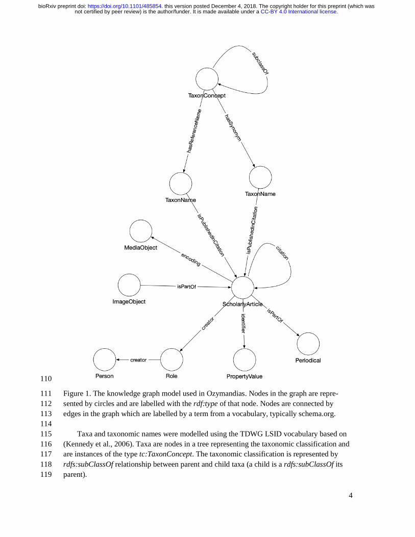
Figure 1. The knowledge graph model used in Ozymandias. Nodes in the graph are repre-111 sented by circles and are labelled with the rdf:type of that node. Nodes are connected by 112 edges in the graph which are labelled by a term from a vocabulary, typically schema.org. 113 114

Taxa and taxonomic names were modelled using the TDWG LSID vocabulary based on 115 (Kennedy et al., 2006). Taxa are nodes in a tree representing the taxonomic classification and 116 are instances of the type tc:TaxonConcept. The taxonomic classification is represented by 117 rdfs:subClassOf relationship between parent and child taxa (a child is a rdfs:subClassOf its 118 parent). 119


https://doi.org/10.1101/485854


5

Taxonomic names (type tn:TaxonName) are connected to the corresponding taxa using 120 relations from the TAXREF vocabulary (Michel et al., 2017) and are typically either accepted 121 names or synonyms. This vocabulary was adopted to because it enables a more direct way of 122 expressing the relationship between taxa and taxonomic names than is possible using the 123 TDWG LSID vocabulary. 124

125 Taxonomic names are published in publications, which were represented using terms 126

from the schema.org vocabulary. In cases where the full text of an article is available as a 127 PDF file I make use of the schema:encoding property to link the publication to a 128 schema:MediaObject representing the PDF. Articles are linked to the journals they were pub-129 lished in by the schema:isPartOf property. 130

131 Representing ordered lists in RDF is not straightforward, which presents a challenge for 132

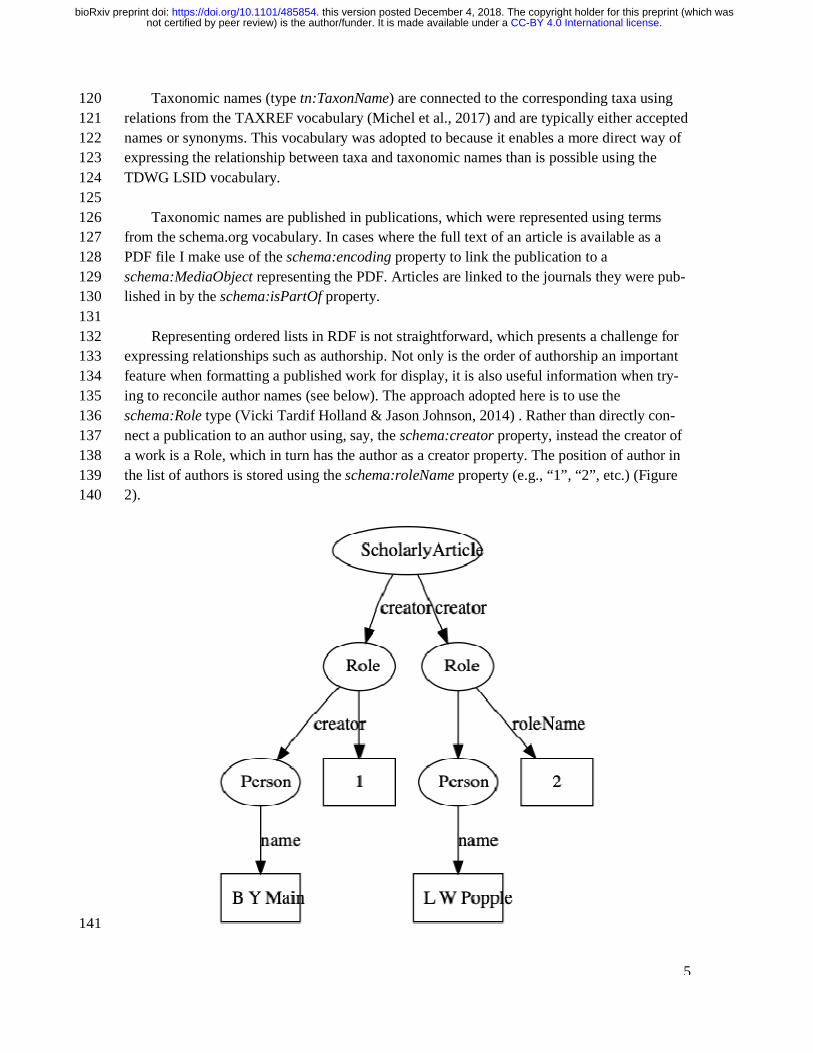
expressing relationships such as authorship. Not only is the order of authorship an important 133 feature when formatting a published work for display, it is also useful information when try-134 ing to reconcile author names (see below). The approach adopted here is to use the 135 schema:Role type (Vicki Tardif Holland & Jason Johnson, 2014) . Rather than directly con-136 nect a publication to an author using, say, the schema:creator property, instead the creator of 137 a work is a Role, which in turn has the author as a creator property. The position of author in 138 the list of authors is stored using the schema:roleName property (e.g., “1”, “2”, etc.) (Figure 139 2). 140

141


https://doi.org/10.1101/485854


6

Figure 2. An example of modelling order of authorship using schema:Role. Each author is 142 linked to the article they authored via a schema:Role node, which specifies the order of au-143 thorship for each author. In this example, “B Y Main” is the first author, “L W Popple” is the 144 second author. 145 146

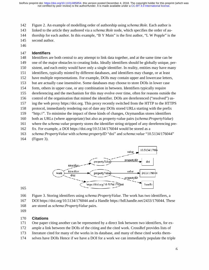
Identifiers 147 Identifiers are both central to any attempt to link data together, and at the same time can be 148 one of the major obstacles to creating links. Ideally identifiers should be globally unique, per-149 sistent, and each entity would have only a single identifier. In reality, entities may have many 150 identifiers, typically minted by different databases, and identifiers may change, or at least 151 have multiple representations. For example, DOIs may contain upper and lowercase letters, 152 but are actually case insensitive. Some databases may choose to store DOIs in lower case 153 form, others in upper case, or any combination in between. Identifiers typically require 154 dereferencing and the mechanism for this may evolve over time, often for reasons outside the 155 control of the organisation that minted the identifier. DOIs are dereferenced (“resolved”) us-156 ing the web proxy https://doi.org. This proxy recently switched from the HTTP to the HTTPS 157 protocol, immediately rendering out of date any DOIs stored URLs starting with the prefix 158 “http://”. To minimise the impact of these kinds of changes, Ozymandias stores identifiers 159 both as URLs (where appropriate) but also as property-value pairs (schema:PropertyValue) 160 where the schema:value property stores the identifier string stripped of any dereferencing pre-161 fix. For example, a DOI https://doi.org/10.5134/176044 would be stored as a 162 schema:PropertyValue with schema:propertyID “doi” and schema:value “10.5134/176044” 163 (Figure 3). 164

165

Figure 3. Storing identifiers using schema:PropertyValue. The work has two identifiers, a 166 DOI https://doi.org/10.5134/176044 and a Handle https://hdl.handle.net/2433/176044. These 167 are stored as schema:PropertyValue pairs. 168 169

Citations 170 One paper citing another can be represented by a direct link between two identifiers, for ex-171 ample a link between the DOIs of the citing and the cited work. CrossRef provides lists of 172 literature cited for many of the works in its database, and many of these cited works them-173 selves have DOIs Hence if we have a DOI for a work we can immediately populate the triple 174


https://doi.org/10.1101/485854


7

store with citation links. This works well if both works have a DOI, but many taxonomically 175 relevant works do not have these identifiers. Even for those works that do have DOIs, these 176 may not have been available at the time the citing work was deposited by a publisher, for ex-177 ample, if the cited work has only recently been assigned a DOI. 178 179

To expand the citation links beyond just those works with DOIs I also generated an iden-180 tifier for each work modelled on the Serial Item and Contribution Identifier (SICI). This iden-181 tifier comprised the International Standard Serial Number (ISSN) of the journal, together with 182 the volume, and the starting page. This triple uniquely identifies most articles, and is easy to 183 generate. SICIs were generated for works harvested from the Australian Faunal Directory, and 184 from the lists of literature cited obtained from CrossRef, and were stored as 185 schema:PropertyValue pairs in the same way as DOIs and other identifiers. By matching SI-186 CIs it was possible to expand citation links beyond those where both works had DOIs. 187

188

Populating the knowledge graph 189 Perhaps the biggest challenge in constructing a knowledge graph is to map names or descrip-190 tions of entities to one or more globally unique identifiers. In some cases the sources data will 191 already have identifiers. Taxa in the ALA each have a unique identifier (a LSID), as do taxa 192 and publications in the AFD (which use UUIDs). The ALA and AFD share the same taxon 193 identifiers, which makes linking the two databases straightforward. However, these identifiers 194 are local in the sense that they are primary keys for local databases that have been converted 195 into URLs. The knowledge graph can only grow if we use external identifiers that are shared 196 by other databases, or at least map local identifiers onto those external identifiers. For publi-197 cations this is straightforward in the sense that a publication in a database of Australian ani-198 mals can be unambiguously mapped onto the publication in, say, a database for Japanese 199 animals. However, a taxon as defined in the Australian Faunal Directory may not correspond 200 exactly to a taxon with the same name in another. 201 202

Reconciling works 203 For the works in AFD I searched for DOIs using the API provided by CrossRef. If a reference 204 was found the associated DOI was assigned to that reference. CrossRef is not the only regis-205 tration agency for DOIs, there are several others that are used by digital libraries and publish-206 ers, such as DataCite, the multilingual European Registration Agency (mEDRA), and Airiti 207

(華藝數位). Most of these agencies lack the discovery services provided by CrossRef, so for 208

these DOIs I harvested the article metadata using a combination of web services and screen 209 scraping, created a local MySQL database to store the metadata, and used that database to 210 match references to DOIs. This database was also used to match articles to other classes of 211 identifiers, such as Handles and URLs. 212 213

Australian natural history institutions are significant publishers of biodiversity literature, 214 and much of this has been scanned by the Biodiversity Heritage Library in Australia. As a 215 consequence many of the articles in the knowledge graph were available in my BioStor pro-216


https://doi.org/10.1101/485854


8

ject (Page, 2011). Identifiers for these articles were found by matching using the BioStor 217 OpenURL service. 218

219

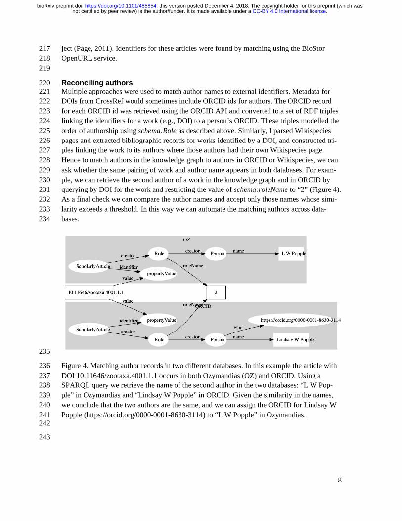
Reconciling authors 220 Multiple approaches were used to match author names to external identifiers. Metadata for 221 DOIs from CrossRef would sometimes include ORCID ids for authors. The ORCID record 222 for each ORCID id was retrieved using the ORCID API and converted to a set of RDF triples 223 linking the identifiers for a work (e.g., DOI) to a person’s ORCID. These triples modelled the 224 order of authorship using schema:Role as described above. Similarly, I parsed Wikispecies 225 pages and extracted bibliographic records for works identified by a DOI, and constructed tri-226 ples linking the work to its authors where those authors had their own Wikispecies page. 227 Hence to match authors in the knowledge graph to authors in ORCID or Wikispecies, we can 228 ask whether the same pairing of work and author name appears in both databases. For exam-229 ple, we can retrieve the second author of a work in the knowledge graph and in ORCID by 230 querying by DOI for the work and restricting the value of schema:roleName to “2” (Figure 4). 231 As a final check we can compare the author names and accept only those names whose simi-232 larity exceeds a threshold. In this way we can automate the matching authors across data-233 bases. 234

235

Figure 4. Matching author records in two different databases. In this example the article with 236 DOI 10.11646/zootaxa.4001.1.1 occurs in both Ozymandias (OZ) and ORCID. Using a 237 SPARQL query we retrieve the name of the second author in the two databases: “L W Pop-238 ple” in Ozymandias and “Lindsay W Popple” in ORCID. Given the similarity in the names, 239 we conclude that the two authors are the same, and we can assign the ORCID for Lindsay W 240 Popple (https://orcid.org/0000-0001-8630-3114) to “L W Popple” in Ozymandias. 241 242

243


https://doi.org/10.1101/485854


9

Data sources 244 I used several different strategies to convert data into the triples required for the knowledge 245 graph. If the source data was in the form of CSV files (e.g., the Australian Faunal Directory) 246 it was imported into a MySQL database, and PHP scripts were written to further clean the 247 data and map it to any external identifiers. Once the data was cleaned and linked, a PHP script 248 was used to export the data in N-triples format. 249 250

Several sources of data (Atlas of Living Australia, CrossRef, ORCID, Wikispecies, and 251 Biodiversity Literature Repository) were accessed via their APIs. For ALA a list of all animal 252 taxa was obtained from the ALA web site, then the JSON record for each taxon was har-253 vested. For CrossRef, data was harvested for just those DOIs found by the bibliographic 254 string to DOI mapping process described above. These DOIs were also submitted to a custom 255 script that queried the ORCID database to discover whether any authors had works with those 256 DOIs in their ORCID profile. If this was the case, the corresponding ORCID profile was 257 downloaded. Each DOI was also used as a query term for searching Wikispecies using its API 258 with the “list” parameter set to “exturlusage” to find wiki pages that mentioned that DOI. 259 Pages found were retrieved in XML format using the API, any references on that page parsed 260 and converted into JSON. All JSON documents obtained from these sources were stored in 261 CouchDB databases and custom CouchDB views were written in Javascript to convert the 262 JSON documents into N-triples. 263

264 By default Ozymandias treats individual publications as a single, monolithic entity. How-265

ever, some publishers such as PLoS and Pensoft provide DOIs for component parts of an arti-266 cle, such as individual figures. (Egloff et al., 2017) have argued that even if a taxonomic arti-267 cle itself is copyrighted, the individual figures are not eligible for copyright, and hence extract 268 and assign DOIs to large numbers of figures extracted from journals such as Zootaxa. These 269 figures, together with ones sourced from open access journals are available through the Bio-270 diversity Literature Repository (“Biodiversity Literature Repository”) (BLR). The BLR is 271 hosted by Zenodo (https://zenodo.org) and each publication and figure has a unique identifier 272 (typically a DOI), and metadata for each publication and figure is available as JSON-LD. This 273 means data from the BLR can be directly incorporated into a triple store. However for this 274 project I wanted just a subset relevant to publications on the Australian fauna, and so I created 275 a CouchDB version of the BLR and write scripts to match publications from the AFD to the 276 corresponding record in the BLR. Metadata for each matching publication and its associated 277 figures were then retrieved directly from Zenodo. 278

279

Knowledge graph 280 The knowledge graph was implemented as a triple store using Blazegraph 2.1.4 running on a 281 Windows 10 server, with a nginx web server acting as a reverse proxy. N-triples for different 282 categories of data (e.g., taxa, publications, etc.) were partitioned using named graphs and up-283 loaded to the triple store. This made it easier to manage sets of data, for example the biblio-284 graphic data could be deleted and reloaded by simply deleting all triples in the corresponding 285


https://doi.org/10.1101/485854


10

named graph, rather than having to delete the entire knowledge graph. It also facilitated some 286 queries, such as author matching across multiple data sources where distinguishing between 287 data source was an essential part of the query. 288 289

Search 290 Being able to simply search for relevant documents by typing in one or more terms is a fea-291 ture users expect from almost any web site. To implement search, basic information on taxa 292 and publications was encoded into a simple JSON document (one per entity) and these JSON 293 documents were indexed using an instance of Elasticsearch 6.3.1 hosted on Google’s Com-294 pute Engine. 295 296

Web interface 297 Designing a semantic web browser to display a richly interconnected data set is a challenging 298 task (Quan & Karger, 2004). For Ozymandias the goal was to have a simple interface which 299 encouraged the user to explore connections between taxa, publications, and people. Apart 300 from the home page, there are two main page types in the web interface for Ozymandias. The 301 first is the search interface which is a simple list of the entities that best match the search 302 terms. Clicking on any member of that list leads to the second page type, which is a display of 303 the entity itself. This display comprises three columns. The left column displays core facts 304 about the entity. These are typically triples that have the entity as their subject, or are one 305 edge away in the knowledge graph (such as thumbnail images), and so can be retrieved from 306 the knowledge graph using either SPARQL DESCRIBE or CONSTRUCT queries. The mid-307 dle column displays connections between the main entity on the page and related entities in 308 the knowledge graph (such as authors of a paper, taxonomic names mentioned in a work, 309 etc.), and is populated by SPARQL queries. The rightmost column is used to display the re-310 sult of searching external sources for information relevant to the entity displayed on the page. 311 Hence, unlike columns one and two, these queries are not SPARQL queries to the local 312 knowledge graph. 313

Results 314 315 Ozymandias can be viewed at https://ozymandias-demo.herokuapp.com. Source code is avail-316 able on GitHub https://github.com/rdmpage/ozymandias-demo. Below I describe the web in-317 terface to Ozymandias, and outline some of the exploratory analyses that can be undertaken 318 using the underlying knowledge graph. Where the results are based on SPARQL queries, 319 those queries are listed in the Supplementary material. 320 321

Web interface 322 A screenshot of the web interface is shown in Figure 5. This shows the three-column layout 323 used to display an entity, its relationships within the knowledge graph, and any known exter-324 nal relationships. 325


https://doi.org/10.1101/485854


11

326

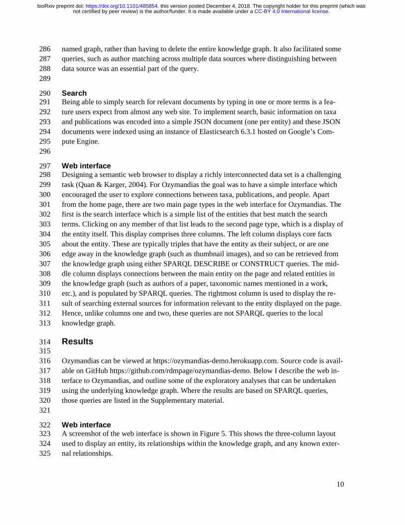
327 Figure 5. Web interface to Ozymandias knowledge graph displaying information for an arti-328 cle. The left column displays a summary of the article, and a PDF viewer (only available if 329 content is freely accessible). The middle column displays related content from the knowledge 330 graph, such as taxa mentioned in the article. The right column shows the result of searches in 331 external web sites for related information, in this case is displays the identifier for Wikidata 332 item that corresponds to this article. To view this page live go to https://ozymandias-333 demo.herokuapp.com/?uri=https://biodiversity.org.au/afd/publication/3e0c1402-de05-4227-334 9df3-803e68300623. 335 336

The first example is a publication, in this case (Nakabo, 1982). The first column summa-337 rises basic data about the publication, and if the full text is available it is displayed using ei-338 ther a PDF viewer, or a simple image viewer in the case of scanned images. The second col-339 umn lists taxa associated with the publication. For publications with identifiers such as DOIs 340 the third column displays whether a record with that DOI exists in external sources such as 341 Wikidata and ORCID. 342


https://doi.org/10.1101/485854


12

343

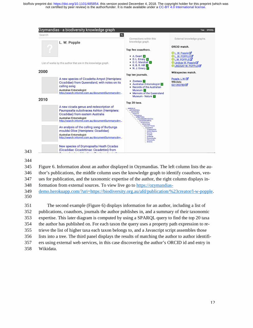
344 Figure 6. Information about an author displayed in Ozymandias. The left column lists the au-345 thor’s publications, the middle column uses the knowledge graph to identify coauthors, ven-346 ues for publication, and the taxonomic expertise of the author, the right column displays in-347 formation from external sources. To view live go to https://ozymandias-348 demo.herokuapp.com/?uri=https://biodiversity.org.au/afd/publication/%23creator/l-w-popple. 349 350

The second example (Figure 6) displays information for an author, including a list of 351 publications, coauthors, journals the author publishes in, and a summary of their taxonomic 352 expertise. This later diagram is computed by using a SPARQL query to find the top 20 taxa 353 the author has published on. For each taxon the query uses a property path expression to re-354 trieve the list of higher taxa each taxon belongs to, and a Javascript script assembles those 355 lists into a tree. The third panel displays the results of matching the author to author identifi-356 ers using external web services, in this case discovering the author’s ORCID id and entry in 357 Wikidata. 358


https://doi.org/10.1101/485854


13

359

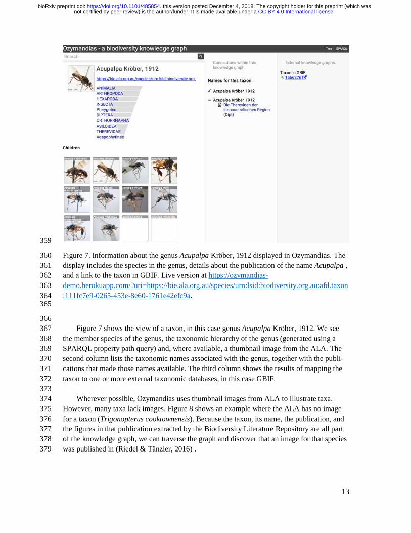
Figure 7. Information about the genus Acupalpa Kröber, 1912 displayed in Ozymandias. The 360 display includes the species in the genus, details about the publication of the name Acupalpa , 361 and a link to the taxon in GBIF. Live version at https://ozymandias-362 demo.herokuapp.com/?uri=https://bie.ala.org.au/species/urn:lsid:biodiversity.org.au:afd.taxon363 :111fc7e9-0265-453e-8e60-1761e42efc9a. 364 365

366 Figure 7 shows the view of a taxon, in this case genus Acupalpa Kröber, 1912. We see 367

the member species of the genus, the taxonomic hierarchy of the genus (generated using a 368 SPARQL property path query) and, where available, a thumbnail image from the ALA. The 369 second column lists the taxonomic names associated with the genus, together with the publi-370 cations that made those names available. The third column shows the results of mapping the 371 taxon to one or more external taxonomic databases, in this case GBIF. 372

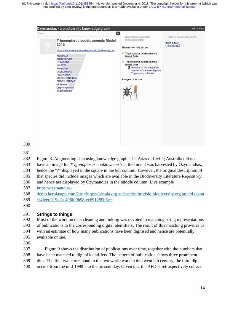
373 Wherever possible, Ozymandias uses thumbnail images from ALA to illustrate taxa. 374

However, many taxa lack images. Figure 8 shows an example where the ALA has no image 375 for a taxon (Trigonopterus cooktownensis). Because the taxon, its name, the publication, and 376 the figures in that publication extracted by the Biodiversity Literature Repository are all part 377 of the knowledge graph, we can traverse the graph and discover that an image for that species 378 was published in (Riedel & Tänzler, 2016) . 379


https://doi.org/10.1101/485854


14

380

381 Figure 8. Augmenting data using knowledge graph. The Atlas of Living Australia did not 382 have an image for Trigonopterus cooktownensis at the time it was harvested by Ozymandias, 383 hence the “?” displayed in the square in the left column. However, the original description of 384 that species did include images which are available in the Biodiversity Literature Repository, 385 and hence are displayed by Ozymandias in the middle column. Live example 386 https://ozymandias-387 demo.herokuapp.com/?uri=https://bie.ala.org.au/species/urn:lsid:biodiversity.org.au:afd.taxon388 :14feec1f-9d2a-496b-9b98-ec691289b5ce. 389 390

Strings to things 391 Most of the work on data cleaning and linking was devoted to matching string representations 392 of publications to the corresponding digital identifiers. The result of this matching provides us 393 with an estimate of how many publications have been digitised and hence are potentially 394 available online. 395 396

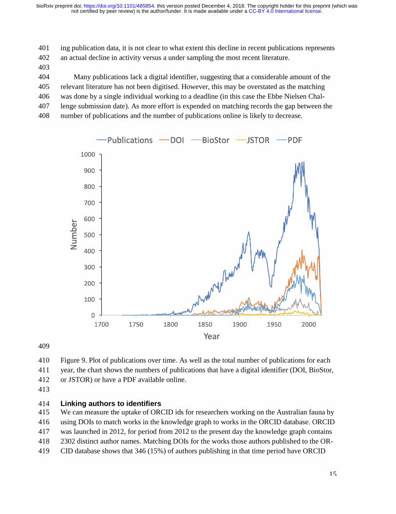
Figure 9 shows the distribution of publications over time, together with the numbers that 397 have been matched to digital identifiers. The pattern of publication shows three prominent 398 dips. The first two correspond to the two world wars in the twentieth century, the third dip 399 occurs from the mid-1990’s to the present day. Given that the AFD is retrospectively collect-400


https://doi.org/10.1101/485854


15

ing publication data, it is not clear to what extent this decline in recent publications represents 401 an actual decline in activity versus a under sampling the most recent literature. 402

403 Many publications lack a digital identifier, suggesting that a considerable amount of the 404

relevant literature has not been digitised. However, this may be overstated as the matching 405 was done by a single individual working to a deadline (in this case the Ebbe Nielsen Chal-406 lenge submission date). As more effort is expended on matching records the gap between the 407 number of publications and the number of publications online is likely to decrease. 408

409

Figure 9. Plot of publications over time. As well as the total number of publications for each 410 year, the chart shows the numbers of publications that have a digital identifier (DOI, BioStor, 411 or JSTOR) or have a PDF available online. 412 413

Linking authors to identifiers 414 We can measure the uptake of ORCID ids for researchers working on the Australian fauna by 415 using DOIs to match works in the knowledge graph to works in the ORCID database. ORCID 416 was launched in 2012, for period from 2012 to the present day the knowledge graph contains 417 2302 distinct author names. Matching DOIs for the works those authors published to the OR-418 CID database shows that 346 (15%) of authors publishing in that time period have ORCID 419


https://doi.org/10.1101/485854


16

ids. This number is likely to be an underestimate as not all works in ORCID have DOIs (and 420 ORCID records sometimes omit DOIs for works that have them), but it suggests limited adop-421 tion of ORCIDs amongst taxonomists and other biodiversity researchers. 422

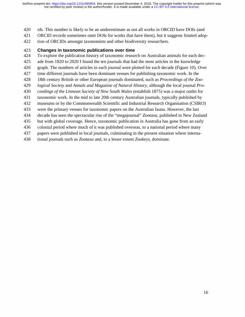
Changes in taxonomic publications over time 423 To explore the publication history of taxonomic research on Australian animals for each dec-424 ade from 1820 to 2020 I found the ten journals that had the most articles in the knowledge 425 graph. The numbers of articles in each journal were plotted for each decade (Figure 10). Over 426 time different journals have been dominant venues for publishing taxonomic work. In the 427 18th century British or other European journals dominated, such as Proceedings of the Zoo-428 logical Society and Annals and Magazine of Natural History, although the local journal Pro-429 ceedings of the Linnean Society of New South Wales (establish 1875) was a major outlet for 430 taxonomic work. In the mid to late 20th century Australian journals, typically published by 431 museums or by the Commonwealth Scientific and Industrial Research Organisation (CSIRO) 432 were the primary venues for taxonomic papers on the Australian fauna. However, the last 433 decade has seen the spectacular rise of the “megajournal” Zootaxa, published in New Zealand 434 but with global coverage. Hence, taxonomic publication in Australia has gone from an early 435 colonial period where much of it was published overseas, to a national period where many 436 papers were published in local journals, culminating in the present situation where interna-437 tional journals such as Zootaxa and, to a lesser extent Zookeys, dominate. 438


https://doi.org/10.1101/485854


17

439

Figure 10. Patterns of publication of taxonomic work on Australian animals 1820-2020. Chart 440 shows the numbers of publications in the top ten journals for each decade. The 19th and early 441 20th centuries are dominated by European journals, by the mid 20th century most taxonomy 442 was published in Australian journals, more recently international journals such as Zootaxa are 443 increasingly important. 444 445 446

Citations and taxonomy as long data 447 Taxonomy is a “long data” discipline (Page, 2016b). In some scientific fields published pa-448 pers have a short citation half-life and hence are relatively ephemeral, quickly losing their 449 relevance as the “research front” moves on (de Solla Price, 1965). The rise of academic 450 search engines such as Google Scholar may increase the discoverability of the older literature 451 (and hence increasing its likelihood of being cited, (Verstak et al., 2014)), but for many fields 452 the older literature fades from importance. In contrast, the taxonomic literature is essentially 453 ageless - any published work is potentially relevant. Part of this relevance reflects the impor-454


https://doi.org/10.1101/485854


18

tance of priority in biological nomenclature, given competing names for the same taxon in 455 general the oldest name wins. Another factor is the sheer number of species and the relative 456 paucity of published knowledge on many of those species. May (1988) estimated that for pub-457 lications in the period 1978 to 1987 for insects there were on average 0.02 papers per species 458 per year, for beetles it was 0.01 papers. Hence a researcher may have to search back through a 459 hundred years of literature in order to find mention of a specific beetle species. 460

461

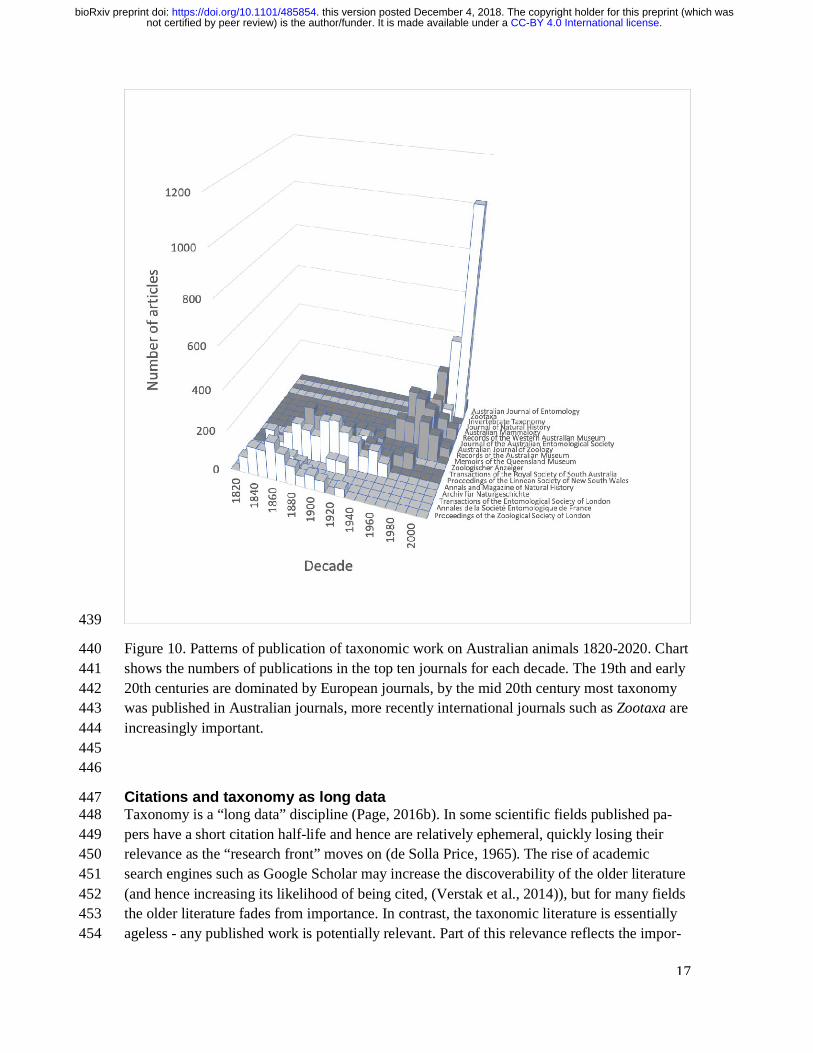
Figure 11. Dates of publication of works cited against the date of publication of the cited 462 work. Each point represents the (x, y) pair (publication date, cited publication date). All cited 463 works must, by definition, be published in the same year or earlier, and hence the points fall 464


https://doi.org/10.1101/485854


19

on or below the diagonal. The few points that are above the diagonal represent errors in 465 CrossRef’s metadata. 466 467

To explore the citation graph for publications on the Australian fauna I queried each cita-468 tion relationship for the dates of publication of the citing and the cited works. The relationship 469 between these two dates (Figure 11) highlights the enduring value of the older taxonomic lit-470 erature. If taxonomic work cited only recent publications then the points in Figure 11would 471 fall on or close to the diagonal. However, even papers published recently (top right of the 472 chart) cite older literature (represented by the vertical columns of dots below each year), and 473 hence much of the area below the diagonal is occupied. 474

475

History of species discovery in different taxonomic groups 476 The knowledge graph enables exploration of the taxonomic history of any taxon of interest. 477 (Pullen, Jennings & Oberprieler, 2014) recently reviewed the history of weevil taxonomy in 478 Australia. Ozymandias has some 3958 accepted weevil species. For each accepted taxon in 479 the ALA classification I used a SPARQL query to retrieve the date the species was originally 480 described, and the dates where then grouped by year. The plot of cumulative numbers of ac-481 cepted species over time (Figure 12) closely matches that reported by Pullen et al. 482


https://doi.org/10.1101/485854


20

483

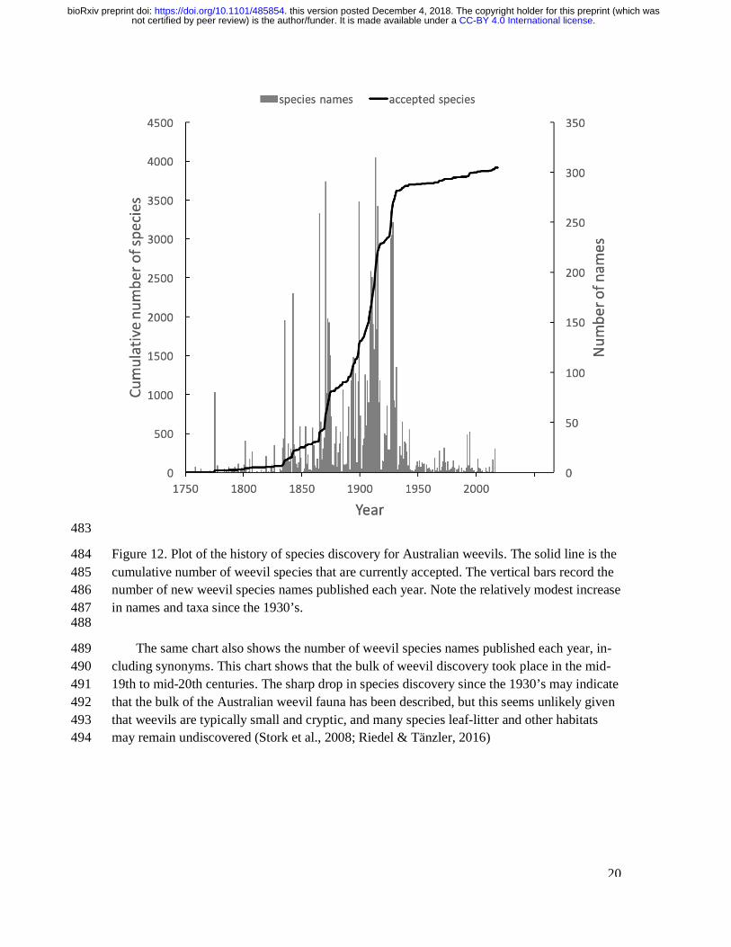
Figure 12. Plot of the history of species discovery for Australian weevils. The solid line is the 484 cumulative number of weevil species that are currently accepted. The vertical bars record the 485 number of new weevil species names published each year. Note the relatively modest increase 486 in names and taxa since the 1930’s. 487 488

The same chart also shows the number of weevil species names published each year, in-489 cluding synonyms. This chart shows that the bulk of weevil discovery took place in the mid-490 19th to mid-20th centuries. The sharp drop in species discovery since the 1930’s may indicate 491 that the bulk of the Australian weevil fauna has been described, but this seems unlikely given 492 that weevils are typically small and cryptic, and many species leaf-litter and other habitats 493 may remain undiscovered (Stork et al., 2008; Riedel & Tänzler, 2016) 494


https://doi.org/10.1101/485854


21

495

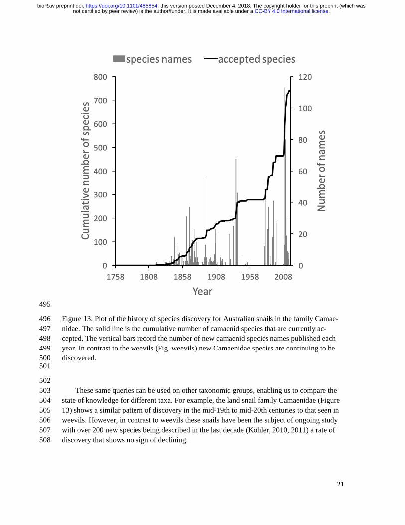
Figure 13. Plot of the history of species discovery for Australian snails in the family Camae-496 nidae. The solid line is the cumulative number of camaenid species that are currently ac-497 cepted. The vertical bars record the number of new camaenid species names published each 498 year. In contrast to the weevils (Fig. weevils) new Camaenidae species are continuing to be 499 discovered. 500 501

502 These same queries can be used on other taxonomic groups, enabling us to compare the 503

state of knowledge for different taxa. For example, the land snail family Camaenidae (Figure 504 13) shows a similar pattern of discovery in the mid-19th to mid-20th centuries to that seen in 505 weevils. However, in contrast to weevils these snails have been the subject of ongoing study 506 with over 200 new species being described in the last decade (Köhler, 2010, 2011) a rate of 507 discovery that shows no sign of declining. 508


https://doi.org/10.1101/485854


22

Discussion 509 Building a knowledge graph requires mapping textual representations of entities to identifiers 510 that are shared across data sources (“strings to things”). Creating this mapping is tedious and 511 time consuming to construct, and in a time limited project such as a challenge entry like 512 Ozymandias the mapping is likely to be incomplete before the deadline for the project. De-513 spite its necessarily incomplete state I think the project illustrates some of the ways a network 514 approach can enrich our knowledge of a topic. The web interface exposes many more connec-515 tions between taxa, publications and people than are evident in the Atlas of Living Australia 516 and Australian Faunal Directory that were used as source databases. 517 518

The underlying knowledge graph can be used to support queries exploring the history of 519 taxonomic publishing and discovery. Some of these queries could be used to help prioritise 520 future work. For example, the pattern of citations (Figure 11) confirms that the older taxo-521 nomic literature is still relevant today, reinforcing the case for digitising the legacy taxonomic 522 literature. We could further explore the citation data to prioritise which journals should be 523 scanned first: for example, by focusing on those journals that have been cited the most. Given 524 that the bulk of taxonomic publications in the 20th century appeared in Australian journals, 525 initiatives such as the Biodiversity Heritage Library in Australia would seem well placed to 526 make the case that this work should be scanned and made openly available. Citation counts 527 can also be used more directly. For example, the International Institute for Species Explora-528 tion annually issues a manually curated list of the “top 10” species discovered the previous 529 year. Such a list could be automatically generated from a knowledge graph using, for exam-530 ple, the number of citations (or other measures of attention) that each work publishing a new 531 species has received. 532

533 Some analyses of the knowledge graph are more focussed on the state of the knowledge 534

graph itself. For example, querying for author identifiers such as ORCIDs reveals a limited 535 uptake of that identifier. This has implications for proposals to use ORCID as the basis for 536 tracking the broader activities of taxonomists, such as specimen collection and identification 537 (Shorthouse). Perhaps the development of such tools may help raise awareness of the possible 538 benefits of authors registering with ORCID. 539

Expanding the knowledge graph 540 The knowledge graph in Ozymandias features only a subset of the entities depicted in earlier 541 work sketching the “biodiversity knowledge graph” (Page, 2013, 2016a). There are several 542 entities that are obvious candidates to be added to Ozymandias, such as specimens and nu-543 cleotide sequences. However, the number of specimens that could potentially be added has 544 implications for the scalability of the knowledge graph. Bearing this in mind, we could add a 545 subset of specimens, such as type specimens, or those which have been sequenced. Fontaine 546 et al. reported that the average lag time between the discovery of a specimen representing a 547 new species and the description of that species is 21 years. The generality of this observation 548 could be evaluated using a knowledge graph that contains both the taxonomic literature and 549 type specimens with dates of collection. 550


https://doi.org/10.1101/485854


23

The Biodiversity Literature Repository highlights the potential of treating scientific arti-551 cles not as monolithic entities but rather as assembles of component parts, including figures. 552 We can drill down further and start to annotate individual parts including fragments of text. 553 The idea of annotating and interlinking fragments of text has a long history, pioneered by 554 people such as Ted Nelson (Douglas R. Dechow & Daniele C. Struppa, 2015), and tools such 555 as Hypotheses.is (“Hypothes.is”) now make this possible. We could view the “micro cita-556 tions” used by taxonomists to specify the page location of a taxonomic name as a form of an-557 notation, hence a logical next step is to map these micro citations onto publications in the 558 knowledge graph so that we can locate these micro citations in the context of the taxonomic 559 literature that they refer to. 560

The future of knowledge graphs 561 To the extent that Ozymandias is judged to be a success it suggests that knowledge graphs 562 have potential to improve the way we aggregate and interface with biodiversity data. How-563 ever, it is worth noting that the biodiversity informatics community has been aware of knowl-564 edge graphs and semantic web technologies for a decade or more, and several taxonomic da-565 tabases have been serving data in RDF since the mid-2000’s. Yet it is hard to point to suc-566 cessful applications of these approaches to the study of biodiversity, and there has been lim-567 ited uptake of linked data beyond a few databases. 568 569

There is a considerable cost involved in cross linking datasets, and to date the rewards for 570 this effort are, perhaps, unclear. At the same time, there is growing concern within biology in 571 general (McDade et al., 2011) and in taxonomy in particular, that existing measures of the 572 output of researchers, such as citations, are poor metrics of activity (cite citation papers). 573 There are also concerns that existing data aggregators do not pay enough attention to tracking 574 the provenance and authorship of information (Franz & Sterner, 2018). Researchers may do 575 much more than write papers, they may clean, prepare, and publish datasets, collect speci-576 mens, curate collections, identify specimens, etc. Keeping track of these activities is greatly 577 facilitated by the use of stable identifiers for people and the objects they work with (e.g., 578 specimens, collections, datasets), and a knowledge graph would be an ideal data structure to 579 quantify the work done, and trace the provenance of data and associated annotations. Projects 580 such as Scholia (Nielsen, Mietchen & Willighagen, 2017) already demonstrate the potential of 581 Wikidata to explore the output of scholars. Hence, it may be that the best way to bootstrap the 582 adoption of biodiversity knowledge graphs is to focus on the implications for being able to 583 give appropriate credit to researchers for all the activities that they undertake. 584

585 There is considerable enthusiasm for the potential of identifiers to help evaluate research 586

(Haak, Meadows & Brown, 2018) and yield insights into the behaviour of researchers 587 (Bohannon, 2017). However, the ease with which measures of research activity (such as cita-588 tion-based measures) switch from being tools for insight into targets to be met suggests we 589 should consider the possibility that metrics developed to create incentives to build knowledge 590 graphs may ultimately harm the researchers being measured. 591

592


https://doi.org/10.1101/485854


24

Beyond internal drivers, such as documenting the provenance of taxonomic information, 593 and quantifying the contributions of researchers, there are also external drivers for consider-594 ing knowledge graphs. Wikidata (Vrandečić & Krötzsch, 2014) is an open, global knowledge 595 graph with an enthusiastic community of editors, and many of the entities taxonomists care 596 about are already included in the graph, such as taxa, people, and publications. This means 597 that we can use Wikidata to help define the scope of a knowledge graph. Anyone constructing 598 a knowledge graph rapidly runs into the problem of scope, in other words, when do you stop 599 adding entities? Once we move beyond specialist knowledge in a given field (such as speci-600 mens, rules of nomenclature, sequences and phylogenies) and include more generic entities 601 that other communities may also be interested in (such as publications, natural history collec-602 tions, people) we reach the point at which we can stop constructing our graph and defer to 603 Wikidata. Hence a key part of the future development of biodiversity knowledge graphs will 604 be to determine the extent to which Wikidata and its community can be responsible for man-605 aging biodiversity-related data. 606


https://doi.org/10.1101/485854


25

Additional Information and Declarations

Competing Interests The author declares he has no competing interests.

Author Contributions Roderic D.M. Page conceived and designed the experiments, performed the experiments, ana-lysed the data, contributed reagents/materials/analysis tools, wrote the paper.

Data Availability The Ozymandias web site is https://ozymandias-demo.herokuapp.com. This site includes a SPARQL interface to query the knowledge graph directly. Source code for the interface is available from GitHub https://github.com/rdmpage/ozymandias-demo. Source code for the scripts used to harvest and clean the data used to populate the knowledge graph is available from https://github.com/rdmpage/oz-afd-export, https://github.com/rdmpage/oz-ala-harvest, https://github.com/rdmpage/oz-csl, and https://github.com/rdmpage/oz-wikispecies.

Funding The work described here was an entry in the Global Biodiversity Information Facility 2018 Ebbe Nielsen Challenge. GBIF had no role in study design, data collection and analysis, deci-sion to publish, or preparation of the manuscript.


https://doi.org/10.1101/485854


26

Acknowledgements Constructing the knowledge graph described here would have been impossible without the wealth of freely available and open source software used in the project. Furthermore, it should be obvious that none of this would have been possible without the centuries of taxonomic re-search by generations of researchers, and the recent efforts to make that research digitally ac-cessible via projects such as Atlas of Living Australia and the Australian Faunal Directory. I’m also indebted to GBIF for running the 2018 Ebbe Nielsen Challenge which gave me a hard deadline to work towards. I also thank Steve Baskauf and Joel Sachs for feedback on the project, and for invitations to present Ozymandias to their colleagues.

References Altmetric. Available at https://www.altmetric.com/ (accessed November 28, 2018). Atlas of Living Australia. Available at https://www.ala.org.au/ (accessed November 27,

2018). Australian Faunal Directory. Available at https://biodiversity.org.au/afd/home (accessed No-

vember 27, 2018). Bebber DP, Wood JRI, Barker C, Scotland RW. 2013. Author inflation masks global capacity

for species discovery in flowering plants. New Phytologist 201:700–706. DOI: 10.1111/nph.12522.

Biodiversity Literature Repository. Available at http://plazi.org/resources/bibliography-of-life-bol/biodiversity-literature-repository-blr/ (accessed November 28, 2018).

Bohannon J. 2017. Vast set of public CVs reveals the world’s most migratory scientists. Sci-ence. DOI: 10.1126/science.aal1189.

Bollacker K, Evans C, Paritosh P, Sturge T, Taylor J. 2008. Freebase: A Collaboratively Cre-ated Graph Database for Structuring Human Knowledge. In: Proceedings of the 2008 ACM SIGMOD International Conference on Management of Data. SIGMOD ’08. New York, NY, USA: ACM, 1247–1250. DOI: 10.1145/1376616.1376746.

Costello MJ, Wilson S, Houlding B. 2013. More Taxonomists Describing Significantly Fewer Species per Unit Effort May Indicate That Most Species Have Been Discovered. Sys-tematic Biology 62:616–624. DOI: 10.1093/sysbio/syt024.

CrossRef. Available at https://www.crossref.org/ (accessed November 27, 2018). Douglas R. Dechow, Daniele C. Struppa (eds.). 2015. Intertwingled: The work and influence

of Ted Nelson. History of Computing. DOI: 10.1007/978-3-319-16925-5. Egloff W, Agosti D, Kishor P, Patterson D, Miller J. 2017. Copyright and the Use of Images

as Biodiversity Data. Research Ideas and Outcomes 3:e12502. DOI: 10.3897/rio.3.e12502.

Franz NM, Sterner BW. 2018. To increase trust, change the social design behind aggregated biodiversity data. Database 2018. DOI: 10.1093/database/bax100.

Godfray HCJ. 2007. Linnaeus in the information age. Nature 446:259–260. DOI: 10.1038/446259a.


https://doi.org/10.1101/485854


27

Grieneisen ML, Zhan Y, Potter D, Zhang M. 2014. Biodiversity, Taxonomic Infrastructure, International Collaboration, and New Species Discovery. BioScience 64:322–332. DOI: 10.1093/biosci/biu035.

Haak LL, Meadows A, Brown J. 2018. Using ORCID, DOI, and Other Open Identifiers in Research Evaluation. Frontiers in Research Metrics and Analytics 3. DOI: 10.3389/frma.2018.00028.

Hypothes.is. Available at https://web.hypothes.is/ (accessed November 28, 2018). Joppa LN, Roberts DL, Pimm SL. 2011. The population ecology and social behaviour of tax-

onomists. Trends in Ecology & Evolution 26:551–553. DOI: 10.1016/j.tree.2011.07.010.

Kennedy J, Hyam R, Kukla R, Paterson T. 2006. Standard Data Model Representation for Taxonomic Information. OMICS: A Journal of Integrative Biology 10:220–230. DOI: 10.1089/omi.2006.10.220.

Köhler F. 2010. Uncovering local endemism in the Kimberley, Western Australia: description of new species of the genus Amplirhagada Iredale, 1933 (Pulmonata: Camaenidae). Records of the Australian Museum 62:217–284. DOI: 10.3853/j.0067-1975.62.2010.1554.

Köhler F. 2011. Descriptions of new species of the diverse and endemic land snail Amplirha-gada Iredale, 1933 from rainforest patches across the Kimberley, Western Australia (Pulmonata: Camaenidae). Records of the Australian Museum 63:167–202. DOI: 10.3853/j.0067-1975.63.2011.1581.

May RM. 1988. How Many Species Are There on Earth? Science 241:1441–1449. DOI: 10.1126/science.241.4872.1441.

McDade LA, Maddison DR, Guralnick R, Piwowar HA, Jameson ML, Helgen KM, Her-endeen PS, Hill A, Vis ML. 2011. Biology Needs a Modern Assessment System for Professional Productivity. BioScience 61:619–625. DOI: 10.1525/bio.2011.61.8.8.

Michel F, Gargominy O, Tercerie S, Faron Zucker C. 2017. A Model to Represent Nomencla-tural and Taxonomic Information as Linked Data. Application to the French Taxo-nomic Register, TAXREF. In: S4Biodiv 2017 - 2nd International Workshop on Se-mantics for Biodiversity co-located with ISWC 2017. Vienna, Austria, 1–12.

Nakabo T. 1982. REVISION OF GENERA OF THE DRAGONETS (PISCES�: CALLIO-NYMIDAE). Publications of the Seto Marine Biological Laboratory 27:77–131. DOI: 10.5134/176044.

Nielsen FÅ, Mietchen D, Willighagen E. 2017. Scholia, Scientometrics and Wikidata. Lecture Notes in Computer Science:237–259. DOI: 10.1007/978-3-319-70407-4_36.

ORCID. Available at https://orcid.org/ (accessed November 27, 2018). Page RD. 2011. Extracting scientific articles from a large digital archive: BioStor and the

Biodiversity Heritage Library. BMC Bioinformatics 12:187. DOI: 10.1186/1471-2105-12-187.

Page RDM. 2013. BioNames: linking taxonomy, texts, and trees. PeerJ 1:e190. DOI: 10.7717/peerj.190.

Page RDM. 2016a. Towards a biodiversity knowledge graph. Research Ideas and Outcomes 2:e8767. DOI: 10.3897/rio.2.e8767.


https://doi.org/10.1101/485854


28

Page RDM. 2016b. DNA barcoding and taxonomy: dark taxa and dark texts. Phil. Trans. R. Soc. B 371:20150334. DOI: 10.1098/rstb.2015.0334.

Pullen KR, Jennings D, Oberprieler RG. 2014. Annotated catalogue of Australian weevils (Coleoptera: Curculionoidea). Zootaxa 3896:1. DOI: 10.11646/zootaxa.3896.1.1.

Quan DA, Karger R. 2004. How to make a semantic web browser. In: ACM Press,. DOI: 10.1145/988672.988707.

Riedel A, Tänzler R. 2016. Revision of the Australian species of the weevil genus Trigonop-terus Fauvel. ZooKeys 556:97–162. DOI: 10.3897/zookeys.556.6126.

Sangster G, Luksenburg JA. 2014. Declining Rates of Species Described per Taxonomist: Slowdown of Progress or a Side-effect of Improved Quality in Taxonomy? Systematic Biology 64:144–151. DOI: 10.1093/sysbio/syu069.

Schema.org. Available at https://schema.org/ (accessed December 3, 2018). Senderov V, Simov K, Franz N, Stoev P, Catapano T, Agosti D, Sautter G, Morris RA, Penev

L. 2018. OpenBiodiv-O: ontology of the OpenBiodiv knowledge management system. Journal of Biomedical Semantics 9. DOI: 10.1186/s13326-017-0174-5.

Shorthouse DP.Bloodhound. Available at https://bloodhound.shorthouse.net (accessed No-vember 28, 2018).

de Solla Price DJ. 1965. Networks of Scientific Papers. Science 149:510–515. DOI: 10.1126/science.149.3683.510.

Stork NE, Grimbacher PS, Storey R, Oberprieler RG, Reid C, Slipinski SA. 2008. What de-termines whether a species of insect is described? Evidence from a study of tropical forest beetles. Insect Conservation and Diversity 1:114–119. DOI: 10.1111/j.1752-4598.2008.00016.x.

Tancoigne E, Ollivier G. 2017. Evaluating the progress and needs of taxonomy since the Convention on Biological Diversity: going beyond the rate of species description. Aus-tralian Systematic Botany 30:326. DOI: 10.1071/sb16017.

Verstak A, Acharya A, Suzuki H, Henderson S, Iakhiaev M, Lin CCY, Shetty N. 2014. On the Shoulders of Giants: The Growing Impact of Older Articles. arXiv:1411.0275 [cs].

Vicki Tardif Holland, Jason Johnson. 2014.Introducing “Role.” Available at http://blog.schema.org/2014/06/introducing-role.html (accessed November 29, 2018).

Vrandečić D, Krötzsch M. 2014. Wikidata. Communications of the ACM 57:78–85. DOI: 10.1145/2629489.

W3C SPARQL Working Group. 2013.SPARQL 1.1 Overview. Available at https://www.w3.org/TR/sparql11-overview/ (accessed November 27, 2018).

Wieczorek J, Bloom D, Guralnick R, Blum S, Döring M, Giovanni R, Robertson T, Vieglais D. 2012. Darwin Core: An Evolving Community-Developed Biodiversity Data Stan-dard. PLoS ONE 7:e29715. DOI: 10.1371/journal.pone.0029715.


https://doi.org/10.1101/485854


29

Supplementary Information

Publications and identifiers Get count of number of published works for each year, and number of works with identifiers. PREFIX xsd: <http://www.w3.org/2001/XMLSchema#> PREFIX rdf: <http://www.w3.org/1999/02/22-rdf-syntax-ns#> SELECT ?work_date (COUNT(?w) as ?c) (COUNT(?doi) as ?c_doi) (COUNT(?biostor) as ?c_biostor) (COUNT(?jstor) as ?c_jstor) (COUNT(?pdf) as ?c_pdf) WHERE { ?w <http://schema.org/datePublished> ?work_date . # just articles ?w <http://www.w3.org/1999/02/22-rdf-syntax-ns#type> <http://schema.org/ScholarlyArticle> . # DOI? OPTIONAL { ?w <http://schema.org/identifier> ?doi . ?doi <http://schema.org/propertyID> "doi" . } # BioStor? OPTIONAL { ?w <http://schema.org/identifier> ?biostor . ?biostor <http://schema.org/propertyID> "biostor" . } # JSTOR? OPTIONAL { ?w <http://schema.org/identifier> ?jstor . ?jstor <http://schema.org/propertyID> "jstor" . } # PDF? OPTIONAL { ?w <http://schema.org/encoding> ?pdf .


https://doi.org/10.1101/485854


30

?pdf <http://schema.org/fileFormat> "application/pdf" . } FILTER regex(?work_date, "^[0-9]{4}$") #FILTER (xsd:integer(?work_date) > 1980) } GROUP BY ?work_date ORDER BY ?work_date

Data in publications.tsv

Journal ranks Query to retrieve top 10 journals for a given decade (in this case 1910) PREFIX rdfs: <http://www.w3.org/2000/01/rdf-schema#> PREFIX tc: <http://rs.tdwg.org/ontology/voc/TaxonConcept#> SELECT ?journal ?issn (COUNT(?journal) AS ?count) WHERE { ?work <http://www.w3.org/1999/02/22-rdf-syntax-ns#type> <http://schema.org/ScholarlyArticle> . ?work <http://schema.org/isPartOf> ?container . ?container <http://schema.org/name> ?journal . ?work <http://schema.org/datePublished> ?year . OPTIONAL { ?container <http://schema.org/issn> ?issn . } FILTER ((xsd:integer(?year) >= 1910) && (xsd:integer(?year) < " . ($year + 9) . ")) } GROUP BY ?journal ?issn ORDER BY DESC(?count) LIMIT 10

Repeat this query for all decades, aggregate results, then filter for journals with > 200 articles. Data in journals.tsv


https://doi.org/10.1101/485854


31

Citation patterns Find all pairs of citing articles and get dates they were published. PREFIX xsd: <http://www.w3.org/2001/XMLSchema#> SELECT ?cited_identifier_type (xsd:integer(?w_year) as ?from) (xsd:integer(?work_year) as ?to) WHERE { ?w <http://schema.org/identifier> ?identifier . ?w <http://schema.org/name> ?w_name . ?w <http://schema.org/datePublished> ?w_year . # Identifier (e.g., DOI) for work we are displaying ?identifier <http://schema.org/value> ?identifier_value . ?citing_identifier <http://schema.org/value> ?identifier_value . ?citing <http://schema.org/identifier> ?citing_identifier . # What does this work cite (typically from CrossRef data) ?citing <http://schema.org/citation> ?cited . # Translate the citing work\'s DOI (or other identifier) into AFD identifier # Get identifier (typically a DOI) for citing work ?cited <http://schema.org/identifier> ?cited_identifier . ?cited_identifier <http://schema.org/value> ?cited_identifier_value . ?cited_identifier <http://schema.org/propertyID> ?cited_identifier_type . # Get work(s) with this identifer (may have > 1 if we have CrossRef record in our triple store ?work_identifier <http://schema.org/value> ?cited_identifier_value . ?work <http://schema.org/identifier> ?work_identifier . ?work <http://schema.org/name> ?name . ?work <http://schema.org/datePublished> ?work_year . # Just include citing records that are also in ALA


https://doi.org/10.1101/485854


32

FILTER regex(str(?work),\'biodiversity.org.au\') . FILTER regex(str(?w),\'biodiversity.org.au\') . FILTER regex(?w_year, "^[0-9]{4}$") FILTER regex(?work_year, "^[0-9]{4}$") }

Data in cites.tsv

Weevils Number of accepted taxon names per year. PREFIX rdfs: <http://www.w3.org/2000/01/rdf-schema#> SELECT ?year (COUNT(?taxonName) AS ?count) WHERE { VALUES ?root_name {"CURCULIONOIDEA"} ?root <http://schema.org/name> ?root_name . ?child rdfs:subClassOf+ ?root . ?child rdfs:subClassOf ?parent . ?child <http://schema.org/name> ?child_name . ?parent <http://schema.org/name> ?parent_name . ?child <http://taxref.mnhn.fr/lod/property/hasReferenceName> ?taxon-Name . ?taxonName <http://rs.tdwg.org/ontology/voc/TaxonName#rankString> "spe-cies" . ?taxonName <http://rs.tdwg.org/ontology/voc/TaxonName#year> ?year . } GROUP BY ?year ORDER BY ?year

Sum these to generate cumulative total. Number of weevil names published each year:


https://doi.org/10.1101/485854


33

PREFIX rdfs: <http://www.w3.org/2000/01/rdf-schema#> SELECT ?year (COUNT(DISTINCT ?name) AS ?c) WHERE { VALUES ?root_name {"CURCULIONOIDEA"} ?root <http://schema.org/name> ?root_name . ?child rdfs:subClassOf+ ?root . ?child rdfs:subClassOf ?parent . ?child <http://schema.org/name> ?child_name . ?parent <http://schema.org/name> ?parent_name . ?child <http://taxref.mnhn.fr/lod/property/hasReferenceName>|<http://taxref.mnhn.fr/lod/property/hasSynonym> ?taxonName . ?taxonName <http://rs.tdwg.org/ontology/voc/TaxonName#rankString> "spe-cies" . ?taxonName <http://schema.org/name> ?name . ?taxonName <http://rs.tdwg.org/ontology/voc/TaxonName#year> ?year . } GROUP BY ?year ORDER BY ?year Combined data in weevils.tsv

Snails Number of accepted taxon names per year PREFIX rdfs: <http://www.w3.org/2000/01/rdf-schema#> SELECT ?year (COUNT(?taxonName) AS ?count) WHERE { VALUES ?root_name {"CAMAENIDAE"} ?root <http://schema.org/name> ?root_name . ?child rdfs:subClassOf+ ?root . ?child rdfs:subClassOf ?parent . ?child <http://schema.org/name> ?child_name . ?parent <http://schema.org/name> ?parent_name .


https://doi.org/10.1101/485854


34

?child <http://taxref.mnhn.fr/lod/property/hasReferenceName> ?taxon-Name . ?taxonName <http://rs.tdwg.org/ontology/voc/TaxonName#rankString> "spe-cies" . ?taxonName <http://rs.tdwg.org/ontology/voc/TaxonName#year> ?year . } GROUP BY ?year ORDER BY ?year

Sum these to generate cumulative total. Number of snail names published each year: PREFIX rdfs: <http://www.w3.org/2000/01/rdf-schema#> SELECT ?year (COUNT(DISTINCT ?name) AS ?c) WHERE { VALUES ?root_name {"CAMAENIDAE"} ?root <http://schema.org/name> ?root_name . ?child rdfs:subClassOf+ ?root . ?child rdfs:subClassOf ?parent . ?child <http://schema.org/name> ?child_name . ?parent <http://schema.org/name> ?parent_name . ?child <http://taxref.mnhn.fr/lod/property/hasReferenceName>|<http://taxref.mnhn.fr/lod/property/hasSynonym> ?taxonName . ?taxonName <http://rs.tdwg.org/ontology/voc/TaxonName#rankString> "spe-cies" . ?taxonName <http://schema.org/name> ?name . ?taxonName <http://rs.tdwg.org/ontology/voc/TaxonName#year> ?year . } GROUP BY ?year ORDER BY ?year


https://doi.org/10.1101/485854


35

Combined data in snails.tsv

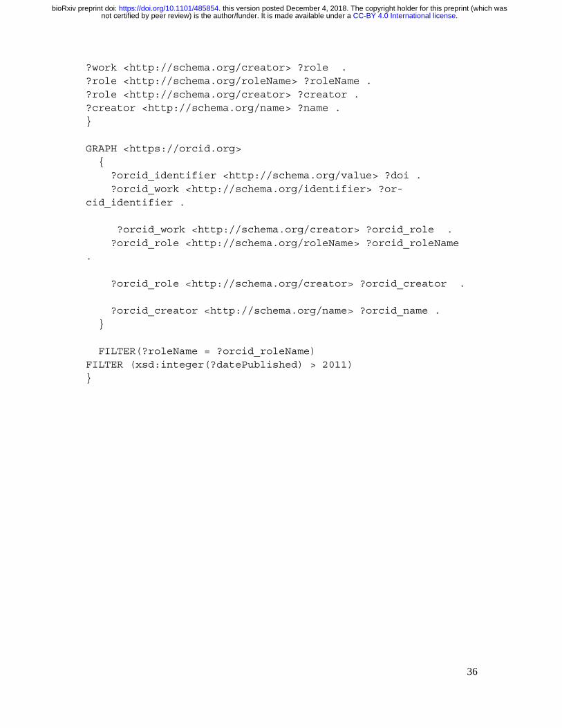
Authors and ORCIDs How many authors of works with DOIs post 2011? SELECT (COUNT(DISTINCT ?creator) as ?c) WHERE { GRAPH <https://biodiversity.org.au/afd/publication> { ?work <http://schema.org/identifier> ?identifier . ?identifier <http://schema.org/propertyID> "doi" . ?identifier <http://schema.org/value> ?doi . ?work <http://schema.org/datePublished> ?datePublished . ?work <http://schema.org/creator> ?role . ?role <http://schema.org/roleName> ?roleName . ?role <http://schema.org/creator> ?creator . ?creator <http://schema.org/name> ?name . } FILTER (xsd:integer(?datePublished) > 2011) }

How many authors of works with DOIs post 2011 had an ORCID? SELECT DISTINCT ?orcid_creator WHERE { GRAPH <https://biodiversity.org.au/afd/publication> { ?work <http://schema.org/identifier> ?identifier . ?identifier <http://schema.org/propertyID> "doi" . ?identifier <http://schema.org/value> ?doi . ?work <http://schema.org/datePublished> ?datePublished .


https://doi.org/10.1101/485854


36

?work <http://schema.org/creator> ?role . ?role <http://schema.org/roleName> ?roleName . ?role <http://schema.org/creator> ?creator . ?creator <http://schema.org/name> ?name . } GRAPH <https://orcid.org> { ?orcid_identifier <http://schema.org/value> ?doi . ?orcid_work <http://schema.org/identifier> ?or-cid_identifier . ?orcid_work <http://schema.org/creator> ?orcid_role . ?orcid_role <http://schema.org/roleName> ?orcid_roleName . ?orcid_role <http://schema.org/creator> ?orcid_creator . ?orcid_creator <http://schema.org/name> ?orcid_name . } FILTER(?roleName = ?orcid_roleName) FILTER (xsd:integer(?datePublished) > 2011) }


https://doi.org/10.1101/485854


Ozymandias: A biodiversity knowledge graph111 Figure 1. The knowledge graph model used in...

Documents

Transcript of Ozymandias: A biodiversity knowledge graph111 Figure 1. The knowledge graph model used in...