Overview of Causal Reasoning with CausalR Hypothesis ...€¦ · Table 1 is an example of the...

Overview of Causal Reasoning with CausalR :

Hypothesis Scoring and P-value Calculation

Steven J Barrett, Glyn Bradley

April 27, 2020

Contents

1 Introduction 3

2 Loading Input Network and Experimental Data 4

3 Computing Score: Multiple Causal Hypotheses 9

4 Computing Score: Specific Causal Hypothesis 10

4.1 Hypothesis-specific CCGs . . . . . . . . . . . . . . . . . . . . 12

5 Scoring 13

5.1 Example Causal hypothesis to be Scored . . . . . . . . . . . . 14

5.2 Network Predictions based upon Hypothesis Node0+ . . . . . 14

5.3 Scoring Calculation . . . . . . . . . . . . . . . . . . . . . . . . 14

6 Hypothesis Score Significance Calculation 15

6.1 Calculation of p-value . . . . . . . . . . . . . . . . . . . . . . 15

6.2 Calculation of Enrichment p-value . . . . . . . . . . . . . . . 16

6.3 Efficiency and Accuracy of Significance Calculation . . . . . . 17

7 Sequential Causal Analysis of Networks (SCAN) 19

8 Visualising the Network of Nodes explained by a SpecificHypothesis 24

8.1 Indirect Individual Hypothesis Network Generation . . . . . . 24

1

8.2 Indirect Network Generation for All Hypotheses found Com-mon across SCAN Deltas . . . . . . . . . . . . . . . . . . . . 25

8.3 Direct Network Generation for All Hypotheses found Com-mon across SCAN Deltas . . . . . . . . . . . . . . . . . . . . 26

9 Additional Usability Features 27

9.1 Automated File Naming . . . . . . . . . . . . . . . . . . . . . 27

9.2 Output Suppression, Re-direction and Quiet Mode . . . . . . 27

9.3 Operating Systems . . . . . . . . . . . . . . . . . . . . . . . . 28

9.4 Parallelisation . . . . . . . . . . . . . . . . . . . . . . . . . . . 28

9.5 Network Filtering . . . . . . . . . . . . . . . . . . . . . . . . . 28

Appendices 30

A Command Sequence Listing for Examples . . . . . . . . . . . 30

B Speeding-up CausalR Processing . . . . . . . . . . . . . . . . 34

2

1 Introduction

CausalR provides causal reasoning (causal network analysis) methods forthe Bioconductor project, enabling the prediction of regulators of sets ofobserved endpoints (e.g. genome scale expression measurements) by inte-gration with prior knowledge in the form of a causal interaction network.Predicted regulators (hypotheses) are assigned a score reflecting their fitwith the input differiential experimental data. Two levels of signmificanceare computed for each hypothesis.

Table 1 is an example of the ranked hypotheses output of CausalR, pro-duced by executing functions CreateCCG(), ReadExperimentalData() thenRankTheHypotheses() on the example causal network and experimentaldata used in the following text.

Node Regulation Score Correct Incorrect Ambiguous p-value Enrichmentp-value

Node0 1 4 5 1 1 0.114 1

Node1 1 3 3 0 0 0.121 1

Node3 1 1 1 0 0 0.500 0.875

Node5 -1 1 1 0 0 0.375 0.875

Node6 -1 1 1 0 0 0.375 0.875

Node7 -1 1 1 0 0 0.375 0.875

Node2 1 0 2 2 0 0.629 0.5

Node4 1 0 0 0 0 0.625 1

Node2 -1 0 2 2 0 0.543 0.5

Node4 -1 0 0 0 0 0.500 1

Node5 1 -1 0 1 0 1 0.875

Node6 1 -1 0 1 0 1 0.875

Node7 1 -1 0 1 0 1 0.875

Node3 -1 -1 0 1 0 1 0.875

Node1 -1 -3 0 3 0 0.957 1

Node0 -1 -4 1 5 1 0.971 1

Table 1: CausalR delta=2 output for example inputs.

Reconstruction of regulatory networks from either newly predicted of pre-vious known regulators of the input experimental data is facilitated, out-putting .sif network and annotation files for visualisation in Cytposcape.

3

The SCAN (Sequential Causal Analysis of Netwroks) methodology of lim-ited false positives in the prediction of regulators is also provided. For furtherbackground on methodological details, suggested analysis approaches and anactual biological causal network, see Bradley and Barrett [submitted].

The following tutorial text provides a step-by-step series of examples on us-ing CausalR, together with further descriptive explanation of what is hap-pening at each stage. For convenience, the complete set of commands, withdetails of further functionality, are listed in Appendix A in the form of anR script.

2 Loading Input Network and Experimental Data

After starting the R environment (either the standard R console or viaan IDE such as Rstudio, http://www.rstudio.com), and setting the workingdirectory to an appropriate location for accessing input files, proceed toloading the CausalR library,

library(CausalR)

The loading of the main package also performs

library(igraph)

since igraph contains network analysis functionality required by CausalR.

These triples represent the network to be used in the example processing,

Node0 Activates Node1

Node0 Inhibits Node2







Each line triple represents a directed edge in the input network of Figure 1.

4

Figure 1: Example input network.

This is read from tab-separated (Cytoscape .sif format) file by one of twouser functions, CreateCG() or CreateCCG() which respectively create andstore either a causal or a computational causal graph. To understand whatthese are we first show how the function CreateCG() is used to create aninternal representation of the network as a Causal Graph (CG).

cg <- CreateCG(system.file( "extdata", "testNetwork1.sif",

package="CausalR"))

## [1] "File read complete - read in 8 lines. Now constructing network"

## [1] "Network has been created - now adding edge properties"

## [1] "Added weights to edges"

The CG is stored in the workspace as an igraph object, which is a par-ticular type of object that can be used to store and process graphs in R(see http://igraph.org/r/doc/igraph.pdf ). The Causal Graph can then bevisualised via,

PlotGraphWithNodeNames(cg) # producing the following graph.

5

Node0

Node1

Node2

Node3

Node4

Node5

Node6

Node7

Note that although only directional connectivity is shown, edge sign attri-bution of the input network is retained. Note also that igraph will assigninternal numeric nodeIDs (for simplicity, the example network here mirrorsthese) that are used internally by CausalR functions. Most CausalR func-tions will automatically convert igraph nodeIDs back to node names recog-nisable to the user, but there are exceptions that return output with thesenumbers. For those outputs, the user will need to apply the GetNodeName().

The CreateCCG() function creates in the workspace an igraph object (hereassigned to ”ccg”) which contains a computational causal network represen-tation of the contents of the input network.sif file.

6

ccg <- CreateCCG(system.file( "extdata", "testNetwork1.sif",

package="CausalR"))

The latter is employed internally instead of a CG for processing efficiency.

A CCG contains double the nodes and vertices, to separately represent upand down regulation of each node, and these are connected according to theoriginal edge relations from the network.sif file. The Computational CausalGraph (CCG) for the input network input can be visualised via,

PlotGraphWithNodeNames(ccg) # producing the following graph.

Node0+

Node1+

Node2+

Node3+Node4+

Node5+

Node6+

Node7+

Node0−

Node1−

Node2−

Node3−Node4−

Node5−

Node6−

Node7−

7

The input differential experimental results (used in subsequent worked ex-amples) is as follows,

Node0 1

Node1 1

Node2 1

Node3 1

Node4 0

Node5 -1

Node6 -1

Node7 -1

In the second column, 1 represents differential activation, -1 differential in-hibition and 0 indicates no differential regulation was observed for the entityrepresented by the node.

The inclusion of all non-differential results is critical to accurate significancecalculations (in their absence CausalR will otherwise see them as not mea-sured and process them accordingly).

A tab-separated file containing this content is read into the workspace usingReadExperimentalData(), as follows,

experimentalData <- ReadExperimentalData(system.file( "extdata",

"testData1.txt", package="CausalR"),ccg)

At this stage checks are performed to identify entities (nodes) not presentwithin the CG/CCG.

These are flagged to the user and excluded from the two column experimen-tal data matrix [igraph nodeID, regulation] that is stored in the workspacefor subsequent processing.

8

3 Computing Score: Multiple Causal Hypotheses

To compute a list of score-ranked hypotheses within an interactive session,the user would employ the RankTheHypotheses() function as follows,

options(width=120)

RankTheHypotheses(ccg, experimentalData, delta=2)

## Number of Nodes to analyse: 8

## NodeID Regulation Score Correct Incorrect Ambiguous p-value Enrichment p-value

## Node0+ 1 1 4 5 1 1 0.1142857 1.000

## Node1+ 2 1 3 3 0 0 0.1214286 1.000

## Node3+ 4 1 1 1 0 0 0.5000000 0.875

## Node5- 6 -1 1 1 0 0 0.3750000 0.875

## Node6- 7 -1 1 1 0 0 0.3750000 0.875

## Node7- 8 -1 1 1 0 0 0.3750000 0.875

## Node2+ 3 1 0 2 2 0 0.6285714 0.500

## Node4+ 5 1 0 0 0 0 0.6250000 1.000

## Node2- 3 -1 0 2 2 0 0.5428571 0.500

## Node4- 5 -1 0 0 0 0 0.5000000 1.000

## Node5+ 6 1 -1 0 1 0 1.0000000 0.875

## Node6+ 7 1 -1 0 1 0 1.0000000 0.875

## Node7+ 8 1 -1 0 1 0 1.0000000 0.875

## Node3- 4 -1 -1 0 1 0 1.0000000 0.875

## Node1- 2 -1 -3 0 3 0 0.9571429 1.000

## Node0- 1 -1 -4 1 5 1 0.9714286 1.000

RankTheHypotheses() incorporates usability features (see Section 9) andparallelisation is supported (see Appendix B for instructions).

Alternatively, the following is used to output similar (results for both + and- hypotheses will again be generated) for a subset of nodes,

options(width=120)

testlist<-c('Node0','Node2','Node3')

RankTheHypotheses(ccg, experimentalData,

delta=2, listOfNodes=testlist)



## Node0+ 1 1 4 5 1 1 0.1142857 1.000

## Node3+ 4 1 1 1 0 0 0.5000000 0.875

## Node2+ 3 1 0 2 2 0 0.6285714 0.500

## Node2- 3 -1 0 2 2 0 0.5428571 0.500

## Node3- 4 -1 -1 0 1 0 1.0000000 0.875

## Node0- 1 -1 -4 1 5 1 0.9714286 1.000

RankTheHypotheses() takes as arguments the workspace CCG and experi-mental matrix object (both from the processing described above), togetherwith a user supplied numeric value for the path length, termed delta, delta.

9

The latter represents the desired number of edges in the network the userwishes the algorithm to look forward, from the hypothesis, to observed resultnodes.

With each further level searched into the network, the number of connectednodes increases roughly exponentially until the delta approximates the net-work average degree. With deltas close to or above the network averagedegree the majority of hypothesis nodes will be connected to most othernodes in the network, and consequently the ability of the scoring algorithmto differentiate good hypotheses from bad ones will be degraded.

RankTheHypotheses() calls the hidden function Scorehypothesis(), whichcomputes scores reflecting the overall level of agreement between predictionsbased upon an individual hypothesis and the experimentally observed resultsfor nodes within delta edges (i.e. to which it can be causally-linked).

4 Computing Score: Specific Causal Hypothesis

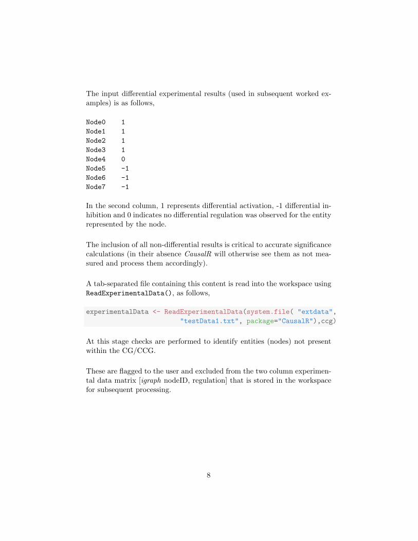
To get scores and significance summary for both up- and down-regulationhypotheses concerning an individual node, the listOfNodes input can beassigned to a sole node name (note that node names are case sensitive inCausalR),

options(width=120)

RankTheHypotheses(ccg, experimentalData, 2, listOfNodes='Node0')



## Node0+ 1 1 4 5 1 1 0.1142857 1

## Node0- 1 -1 -4 1 5 1 0.9714286 1

It may first be useful to check on node content and length of the shortest pathfrom the proposed hypothesis (root) node to any specific (outcome) targetnode(s) of interest. For this the function GetShortestPathsFromCCG() isemployed,

GetShortestPathsFromCCG(ccg, 'Node0', 'Node3')

node0+ node1+ node3+

An alternative to RankTheHypotheses() enables acquisition of further detailon the breakdown of scoring contributions. The MakePredictionsFromCCG()

10

function can be used directly to get scores for a particular signed hypothesisof a node,

predictions <- MakePredictionsFromCCG('Node0',+1,ccg,2)

predictions

## [,1] [,2]

## [1,] 1 1

## [2,] 2 1

## [3,] 3 -1

## [4,] 4 1

## [5,] 5 1

## [6,] 6 0

## [7,] 7 -1

## [8,] 8 -1

The input node0 is the root (or hypothesis) node, +1 is the direction ofregulation, ccg is the network, and the last value, 2, is the delta value(these inputs are explained in more detail in the following section). Thepredictions will be returned as above, with the igraph assigned node ID inthe first column and the direction of regulation in the second.

The ScoreHypothesis() function can then be used to provide a summary ofthe comparisons between the predictions from the given hypothesis againstthe observed outcomes in the experimental data,

ScoreHypothesis(predictions, experimentalData)

## [1] 4 5 1 1

This returns 4 integer values, which (in order) are the score (the number ofcorrect predictions minus the number of incorrect predictions), number ofcorrect predictions, number of incorrect predictions and number of ambigu-ous predictions (these will be explained later within the Scoring Section).

To discover how each predicted node outcome contributes to the score, theCompareHypothesis() function is used to provide a comparison betweenexperiment and prediction for each node separately,

11

GetNodeName(ccg,CompareHypothesis(predictions, experimentalData))

## NodeID Prediction Experiment Score

## 1 Node0 1 1 1

## 2 Node1 1 1 1

## 4 Node3 1 1 1

## 7 Node6 -1 -1 1

## 8 Node7 -1 -1 1

## 5 Node4 1 0 0

## 6 Node5 0 -1 0

## 3 Node2 -1 1 -1

The use of function GetNodeName() is required here to convert igraph nodeIDs,output by CompareHypothesis(), back to user recognisable node names, aswas supplied in the inputs.

Functions CalculateSignificance() and CalculateEnrichmentPValue()

can be used to calculate the statistical significance of a given signed hypoth-esis, as detailed in the R code of Appendix A.

4.1 Hypothesis-specific CCGs

During scoring, hypothesis-specific CCGs are sequentially created and scored.Each hypothesis will be represented as the unique root node of its corre-sponding CCG, whilst the maximum depth for any hypothesisCCG is equalto the path length, delta.

Since each hypothesis observes a either upward or downward regulation, thenumber of individual hypothesisCCGs computed and scored will be equal totwice the number of nodes in the input network, if all possible hypotheses aretested, as this is the default behaviour for function RankTheHypotheses().

Prior to the construction of each hypothesisCCG, nodes beyond delta edgesfrom the hypothesis are removed from the processed network and untestednodes (those without experimental results, apart from the hypothesis nodeitself) are also excluded. To construct the final hypothesisCCG, regulatoryrelations are then applied between the hypothesis along all paths toward theremaining nodes, observing the original network edge values.

12

5 Scoring

To aid scoring the CCG object represents a partitioning of the set of nodesin the experimental data, represented by T |G|, into three sets: the positivelyregulated, negatively regulated and those that are unaffected. These sets aredenoted as Sh+, Sh− and Sh0 respectively, as defined in [2012a].

Thus in the terminology of the Methods: Scoring hypotheses section of[2012a], the observed experimental input (as above) would be representedas :

G+ = {Node0,Node1,Node2,Node3}G− = {Node5,Node6,Node7}G0 = {Node4}

Any node greater than delta edges from the hypothesis node is automat-ically added to Sh0, since the path length to the hypothesis is deemed toodistant to include in scoring, according to user parameterisation.

Figure 2: Network consequences of Node0+

13

5.1 Example Causal hypothesis to be Scored

In the following example calculations, the causal hypothesis to be scoredis up-regulation of Node0, denoted as Node0+. Figure 2 above shows thedownstream consequences of up-regulating Node0, as derived by traversingits hypothesisCCG, observing how the original network edge values translatethe regulatory sign of the (root) hypothesis along the paths to predictedoutcomes. Note that Node 5 is both positively and negatively regulated byNode0+.

5.2 Network Predictions based upon Hypothesis Node0+

The predictions |TGc| from the network (represented as per [2012a], Meth-ods: Scoring hypotheses) would be:

Sh+ = {Node0,Node1,Node3,Node4}Sh− = {Node2,Node6,Node7}Sh0 = {Node5}

5.3 Scoring Calculation

[Example for delta=2] Comparing T |G| to T |Gc| yields the correct predic-tions from this hypothesis as: Node 0, Node 1, Node 3, Node 6 and Node 7.The only incorrect prediction from this hypothesis is: Node 2.

The CausalR scoring algorithm traces the shortest path from hypothesis tooutcome node and then evaluates its sign to achieve a predicted regulationfor that outcome node. The hypothesis here yields a so called ”ambiguous”prediction-outcome match for Node 5, since there are two shortest paths toit and their predictions disagree, hence it doesn’t contribute to the scoring.

Node 4 is also excluded from the score calculation because the observedexperimental outcome for it was non-differentially regulated (unchanged)and this is a result that cannot be predicted by CausalR, as only an up ordown regulation can be inferred from a signed graph.

Subtracting number of incorrect predictions (1) from the number that wascorrect (5) yields a score of 4 for hypothesis Node0+.

14

6 Hypothesis Score Significance Calculation

To account for the scenario where the more heavily connected hypothesisnodes have greater potential to score more highly than less connected ones,the significance of each hypothesis score needs to be individually calculated.

A lower significance (higher p-value) cut-off can then be applied as a filterto the overall scores ranking, as decided via the biological expertise of theuser.

CausalR provides both p-values and enrichment p-values for this purpose.There are two alternatives for p-value calculation: a computationally expen-sive exact ”quartic” algorithm (see section 2.4 in [2012a]) and (for largerinputs) a very much more efficient (minutes instead of hours, hence set asdefault) approximate ”cubic” algorithm (see pages 6-7 in [2012b]).

6.1 Calculation of p-value

[Continuation of previous example for delta=2] Within the context of net-work causal reasoning (see section 2.4, [2012a]), we are looking for theprobability of obtaining a hypothesis (node) score at least as extreme asthat which was observed, assuming the null hypothesis, that the hypothesisnode was not responsible for producing the experimental outcomes, is true(i.e. result is not significantly different from random).

To calculate the p-value significance of this score for hypothesis Node0+,these predictions must be scored against all possible predictions with |G+| =4, and |G− | = 3.

Given that there are 8 nodes to pick each combination from, the total numberof combinations is: 8C4 × 4C3 = 280

There is only one way to get the highest possible score of 7.

There are two approaches to achieve a score of 6. The first is to choose all4 nodes in G+ from the nodes in Sh+, and two of the nodes in G− fromSh−: there are 4C4 x 3C2 = 3 ways of doing this. The other possibility isto choose 3 nodes in Sh+ and 1 in Sh0 as the nodes in G+. Then choose all

15

three of the nodes in G− from Sh− there are 4C3 x 3C3 = 4 ways of doingthis. Hence there are 7 ways of scoring 6 in total.

A score of 5 cannot be achieved.

There are two ways to score 4. (The first is to choose 3 nodes from Sh+ and1 from Sh− as the nodes in G+, then choose 2 nodes from Sh− and the 1 inSh0 as the nodes in G−. There are 4C3 x 3C1 = 12 ways of doing this. Thesecond way is to choose 3 nodes from Sh+ and the 1 from Sh0 as the nodesin G+, then choose 2 nodes from Sh− and 1 in Sh+ as the nodes in G−.There are 4C3 x 3C2 = 12 ways of doing this. This means in total there are24 ways of scoring 4.

We now have all the information we need to calculate the p-value of thehypothesis above. There are 24+7+1 = 32 ways to score 4 or higher, hencethe p-value should be 32/280 = 0.114, as can be seen for the up-regulatednode 0 hypothesis in Table 1.

6.2 Calculation of Enrichment p-value

Enrichment p−values, pE , are calculated using standard approaches usedfor gene ontology enrichment (see [GOEAST])

Where n++ + n+− + n−+ + n−− = m ( i.e. the number of differentiallyexpressed genes, m in Table 2), and T = T |G| is the total number of exper-imental transcripts; then pE is the probability of getting m or more differ-ential nodes from a set of T nodes given the fraction of nodes predicted tobe differential.

This computation is done using the Fisher exact test (see [Fisher]), asimplemented in the fisher.test function in base R.

The goal is to compare the actual number of differential nodes to the numberof predicted ones, given the values of q+, q−, q0, n+, n−, n0, n++, n+−, n−+and n−− in Table 2 below.

16

PredictedCausal Network

MeasuredDifferential

MeasuredNon-differential

MeasuredTotal

DifferentiallyExpressed

n++ +n+−+n−+ +n−− = m n+0 + n−0 q+ + q−

Non-differentiallyExpressed

n0+ + n0− = n+ + n− −m n00 q0

Total n+ + n− n0 T |G|

Table 2: Result outcome categorisations used in significance calculations.

The probability of getting this arrangement of values is given by the hyper-geometric distribution,

p =

(q++q−m

)( q0n0++n0−

)( |T (G)|n++n−

)To obtain pE , the probability of getting m or more elements in the intersec-tion between the sets of predicted versus experimentally-observed differen-tial nodes, needs to be calculated. The formula employed to calculate theenrichment p-value is therefore,

pE =

q++q−∑i=m

(q++q−i

)( q0n++n−−i

)( |T (G)|n++n−

)

6.3 Efficiency and Accuracy of Significance Calculation

As stated earlier, it is crucial to include non-differential outcomes in theexperimental input for accurate significance calculations. The problem withthis is that for large NGS study data compute times increase greatly andmuch of the added effort will be on significance calculations for poor hy-potheses.

This can be avoided by resetting the correctPredictionsThreshold valueused by the RankTheHypotheses() function. This is normally set to minusinfinity, which means that p and pE values will be calculated regardless of

17

hypothesis score. When reset to a positive value it restricts significancecalculations to a subset of hypotheses with a minimum number of correctpredictions (all other hypotheses will automatically get NA values).

options(width=120)

Rankfor4<-RankTheHypotheses(ccg, experimentalData, 2,

correctPredictionsThreshold=4)


Rankfor4 # For example output only


## Node0+ 1 1 4 5 1 1 0.1142857 1

## Node1+ 2 1 3 3 0 0 NA NA

## Node3+ 4 1 1 1 0 0 NA NA

## Node5- 6 -1 1 1 0 0 NA NA

## Node6- 7 -1 1 1 0 0 NA NA

## Node7- 8 -1 1 1 0 0 NA NA

## Node2+ 3 1 0 2 2 0 NA NA

## Node4+ 5 1 0 0 0 0 NA NA

## Node2- 3 -1 0 2 2 0 NA NA

## Node4- 5 -1 0 0 0 0 NA NA

## Node5+ 6 1 -1 0 1 0 NA NA

## Node6+ 7 1 -1 0 1 0 NA NA

## Node7+ 8 1 -1 0 1 0 NA NA

## Node3- 4 -1 -1 0 1 0 NA NA

## Node1- 2 -1 -3 0 3 0 NA NA

## Node0- 1 -1 -4 1 5 1 NA NA

subset(Rankfor4,Correct>=4)


## Node0+ 1 1 4 5 1 1 0.1142857 1

This can also be useful where the user wishes to employ the more compu-tationally expensive exact quartic (1a) algorithm on a subset of interestinghypotheses, instead of using the default cubic (1b) approximation algorithm.

18

7 Sequential Causal Analysis of Networks (SCAN)

Given that true causal regulators are likely to regulate nodes at variousdistances along the pathways in which they feature, the use of a range ofdifferent deltas can be employed to improve enrichment for them. Thiswas the thinking behind Sequential Causal Analysis of Networks (SCAN)approach introduced in Bradley and Barrett [submitted].

By invoking the runSCANR() function, the RankThehypotheses() functionis iteratively run for a range of path lengths (deltas), starting from delta=1

up to the value of the user-supplied variable NumberOfDeltaToScan (defaultis 5), to discover nodes that consistently score in the highest topNumGenes

(default is 150) across all SCAN deltas run.

So for example given the following experimental data,

NodeA 1

NodeB -1

NodeC 1

NodeD -1

NodeE 1

NodeF -1

NodeG 1

NodeH -1

NodeI 1

NodeJ -1

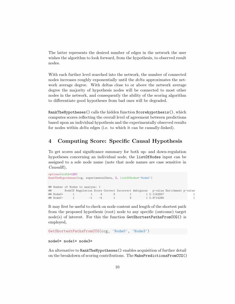
and a more complex network, as in the Cytoscape (http:www.cytoscape.org)depiction of testnet.sif in Figure 3 below).

The runSCANR() function will first write the number of nodes to analyse tothe R console window (this will be repeated for each delta run). Then thenext NumberOfDeltaToScan lines output will list the top hypotheses fromeach delta that was run, whilst the final line gives the SCAN results for thetop hypotheses in common between these deltas.

19

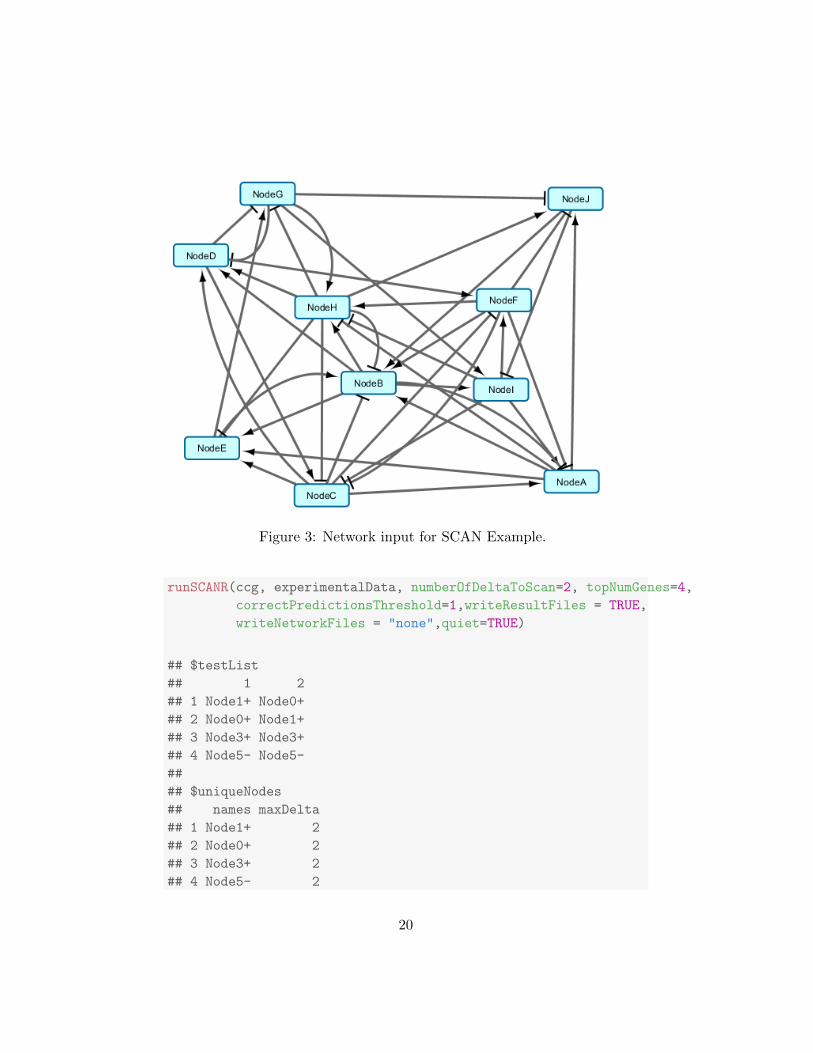
Figure 3: Network input for SCAN Example.

runSCANR(ccg, experimentalData, numberOfDeltaToScan=2, topNumGenes=4,

correctPredictionsThreshold=1,writeResultFiles = TRUE,

writeNetworkFiles = "none",quiet=TRUE)

## $testList

## 1 2

## 1 Node1+ Node0+

## 2 Node0+ Node1+

## 3 Node3+ Node3+

## 4 Node5- Node5-

##

## $uniqueNodes

## names maxDelta

## 1 Node1+ 2

## 2 Node0+ 2

## 3 Node3+ 2

## 4 Node5- 2

20

##

## $commonNodes

## [1] "Node1+" "Node0+" "Node3+" "Node5-"

testList contains the hypotheses found at each delta, as restricted by top-NumGenes.

uniqueNodes contains all hypotheses, with the maximum delta that returnedthem.

commonNodes contains only the hypotheses subset ranked in the first top-NumGenes of all hypotheses across ALL deltas run, and these are ranked inorder found at the highest delta.

Additionally, under the above settings, three files are created in the currentR workspace:

1. A common nodes file: CommonNodes-testNetwork1-testData1-deltaScanned2-top4.txt

Containing:

Node1+

Node0+

Node3+

Node5-

This content is equivalent to that in commonNodes above.

2. A top nodes file: TopNodes-testNetwork1-testData1-deltaScanned2-top4.txt

Containing:

names maxDelta

Node1+ 2

Node0+ 2

Node3+ 2

Node5-2

This content is equivalent to that in uniqueNodes above.

21

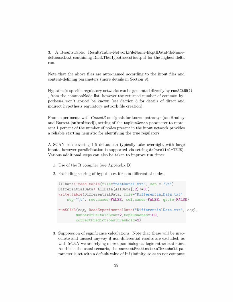
3. A ResultsTable: ResultsTable-NetworkFileName-ExptlDataFileName-deltaused.txt containing RankTheHypotheses()output for the highest deltarun.

Note that the above files are auto-named according to the input files andcontent-defining parameters (more details in Section 9).

Hypothesis-specific regulatory networks can be generated directly by runSCANR()

, from the commonNode list, however the returned number of common hy-potheses won’t apriori be known (see Section 8 for details of direct andindirect hypothesis regulatory network file creation).

From experiments with CausalR on signals for known pathways (see Bradleyand Barrett [submitted]), setting of the topNumGenes parameter to repre-sent 1 percent of the number of nodes present in the input network providesa reliable starting heuristic for identifying the true regulators.

A SCAN run covering 1-5 deltas can typically take overnight with largeinputs, however parallelisation is supported via setting doParallel=TRUE).Various additional steps can also be taken to improve run times:

1. Use of the R compiler (see Appendix B)

2. Excluding scoring of hypotheses for non-differential nodes,

AllData<-read.table(file="testData1.txt", sep = "\t")DifferentialData<-AllData[AllData[,2]!=0,]

write.table(DifferentialData, file="DifferentialData.txt",

sep="\t", row.names=FALSE, col.names=FALSE, quote=FALSE)

runSCANR(ccg, ReadExperimentalData("DifferentialData.txt", ccg),

NumberOfDeltaToScan=2,topNumGenes=100,


3. Suppression of significance calculations. Note that these will be inac-curate and unused anyway if non-differential results are excluded, aswith SCAN we are relying more upon biological logic rather statistics.As this is the usual scenario, the correctPredictionsThreshold pa-rameter is set with a default value of Inf (infinity, so as to not compute

22

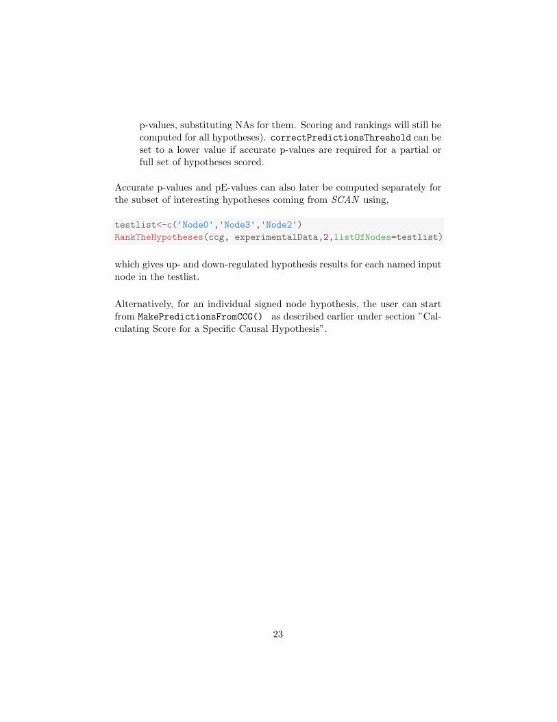
p-values, substituting NAs for them. Scoring and rankings will still becomputed for all hypotheses). correctPredictionsThreshold can beset to a lower value if accurate p-values are required for a partial orfull set of hypotheses scored.

Accurate p-values and pE-values can also later be computed separately forthe subset of interesting hypotheses coming from SCAN using,

testlist<-c('Node0','Node3','Node2')

RankTheHypotheses(ccg, experimentalData,2,listOfNodes=testlist)

which gives up- and down-regulated hypothesis results for each named inputnode in the testlist.

Alternatively, for an individual signed node hypothesis, the user can startfrom MakePredictionsFromCCG() as described earlier under section ”Cal-culating Score for a Specific Causal Hypothesis”.

23

8 Visualising the Network of Nodes explained bya Specific Hypothesis

Hypothesis-specific regulatory sub-networks can be generated indirectly (i.e.after running SCAN) for individual hypotheses or all hypotheses, as well asdirectly via runSCANR() itself.

8.1 Indirect Individual Hypothesis Network Generation

The function WriteExplainedNodesToSifFile() allows production of anetwork of explained nodes, for a particular hypothesis, in .sif file formatfor visualising in Cytoscape. The function is called as follows:

WriteExplainedNodesToSifFile("Node1", +1,ccg,experimentalData,delta=2)

Unless directed elsewhere, this creates six new files in the working directory:

corExplainedNodes-testNetwork1-testData1-delta2-Node1+.sif

corExplainedNodes-testNetwork1-testData1-delta2-Node1+_anno.txt

incorExplainedNodes-testNetwork1-testData1-delta2-Node1+.sif

incorExplainedNodes-testNetwork1-testData1-delta2-Node1+_anno.txt

ambExplainedNodes-testNetwork1-testData1-delta2-Node1+.sif

ambExplainedNodes-testNetwork1-testData1-delta2-Node1+_anno.txt

The correctly explained nodes (corExplainedNodes) .sif file contains inter-actions representing all of the explained nodes (i.e. nodes that have thesame direction of regulation in both the network and the experimental data,as predicted under the hypothesis of up-regulated Node1+, with contentstructured as follows,




The corresponding (corExplainedNodes) annotation file contains the respec-tive explained node regulation values,

24

NodeID Regulation

Node1 1

Node3 1

Node5 -1

These files can be directly loaded into Cytoscape to visualise the regulatorynetwork of hypothesis-explained nodes, such as in figure 4.

Figure 4: Example hypothesis-specific regulatory network (Cytoscape view).

8.2 Indirect Network Generation for All Hypotheses foundCommon across SCAN Deltas

An additional function, WriteAllExplainedNodesToSifFile(), accepts thecommonNodes component of the scanResults workspace object (assigned tostore the runSCANR() output) to generate networks for all the hypothesesfound in common across all SCAN delta settings:

scanResults <- runSCANR(ccg, experimentalData, numberOfDeltaToScan=2,

topNumGenes=4,correctPredictionsThreshold=1,

writeResultFiles = FALSE, writeNetworkFiles = "none",quiet=FALSE)

WriteAllExplainedNodesToSifFile(scanResults, ccg, experimentalData,

delta=2, correctlyExplainedOnly = TRUE, quiet = TRUE)

This produces pairs of corExplainedNodes .sif and annotation network filesfor all hypotheses (Node0+, Node1+, Node3+ and Node5-), in each caseincluding only those experimental data nodes that are correctly explainedby that hypothesis (i.e. as defined by using writeNetworkFiles = ”correct”instead of ”all”).

25

8.3 Direct Network Generation for All Hypotheses foundCommon across SCAN Deltas

The following command shows how to generate the same networks as in thelatter example above, only directly from runSCANR()

runSCANR(ccg, experimentalData, numberOfDeltaToScan=2,

topNumGenes=4,correctPredictionsThreshold=1,quiet=TRUE,

writeResultFiles = TRUE, writeNetworkFiles = "correct")

Files generated in this way get the full input auto-naming, i.e. corExplainedNodes-testNetwork1-testData1-delta2-top4-Node0+.sif, but care needs to be takento sensibly try to restrict the set of common nodes produced by runSCANR()

otherwise there may be very many!

26

9 Additional Usability Features

9.1 Automated File Naming

The RankTheHypotheses() and runSCANR() functions will auto-name theirprimary output files with names that identify all relevant inputs and param-eterisations employed.

These filenames will therefore contain the input network filename, inputexperimental signal filename and the input delta parameter value.

The results table produced by runSCANR() will also feature the topNumGenesparameter value.

All network files output by functions WriteExplainedNodesToSifFile()

and WriteAllExplainedNodesToSifFile() will contain in their filenamethe specified hypothesis node name with the +/- direction of regulation.

9.2 Output Suppression, Re-direction and Quiet Mode

All the functions mentioned in the above section will by default output tothe current R working directory, however they can to configured to sendoutputs to a named directory specified via the outputDir parameter (thiscan accept a path with directory name, if the folder is not to be in workingdirectory). If the specified directory doesn’t exist it will be created.

RankTheHypotheses() and runSCANR() functions have a quiet flag that isset to FALSE by default. Changing this to TRUE will suppress output ofsome or all results to the screen (depending upon other settings;useful forbatch scripted runs).

Similarly, there are flags to suppress results files creation:

RankTheHypotheses() has a writeFile flag set to TRUE so as to write afile by default. When set to FALSE no output files are created (useful whenoutputs are to be stored a workspace object, i.e. via assignment using the<- assignment operator.

runSCANR() has a writeResultsFiles flag which works in a similar wayto control writing of the usual SCAN text file outputs. The default TRUE

setting will result in three text files. FALSE will switch this off, i.e. for whenresults are directed into the R workspace via assignment to an object.

RunSCANR() also accepts a further writeNetworkFiles flag for control ofautomated regulator network files generation. This is set to all by default.

27

9.3 Operating Systems

CausalR as a Bioconductor package has been built for Linux, PC and Macoperating systems. Operation and functionality is identical regardless of theOS used.

9.4 Parallelisation

The RankTheHypotheses() and RunSCANR() functions are fully parallelised.Parallelisation can be switched-on by including doParallel=TRUE in theirparameters. The user can optionally specify the number of cores by settingthe numCores flag to an integer value (default is NULL, whereby the number ofavailable cores will be automatically detected) . See Appendix B for furtheradvice on speeding-up CausalR processing.

9.5 Network Filtering

The CreateCCG() function can read an optional node inclusion text filecontaining a list of node names to filter the network interactions against.The direction of filtering is controlled by an optional excludeNodesInFileparameter to specifiy including (excludeNodesInFile=FALSE) only thosetext file nodes (and their interactions) in the CCG network object, or to(default setting) exclude those nodes from all interactions in the CCG.

CreateCCG(filename, nodeInclusionFile = 'NodesList.txt',

excludeNodesInFile = TRUE)

Note that both the influencing and influenced nodes will be searched againstacross all interactions within the input network. Individual interactions willbe included or excluded if one (or both) node name(s) match against anyspecified within the node inclusion file.

28

References

[1] Bradley, G. and Barrett, S.J. (submitted) CausalR: extracting mechanis-tic sense from genome scale data. Bioinformatics, application note.

[2] Chindelevitch, L. et al. (2012a) Causal reasoning on biological networks:interpreting transcriptional changes. Bioinformatics, 28(8):1114-21.

[3] Chindelevitch, L. et al. (2012b) Assessing statistical significance in causalgraphs (Methodology article). BMC Bioinformatics, 13:35- 48.

[4] Fischer, R. A. (1970) Statistical Methods for Research Workers. Oliver& Boyd.

[5] Zheng, Q. and Wang, X-J. (2008) GOEAST: a web-based software toolkitfor Gene Ontology enrichment analysis. Nucleic Acids Research, 36,W358–W363.

29

Appendices

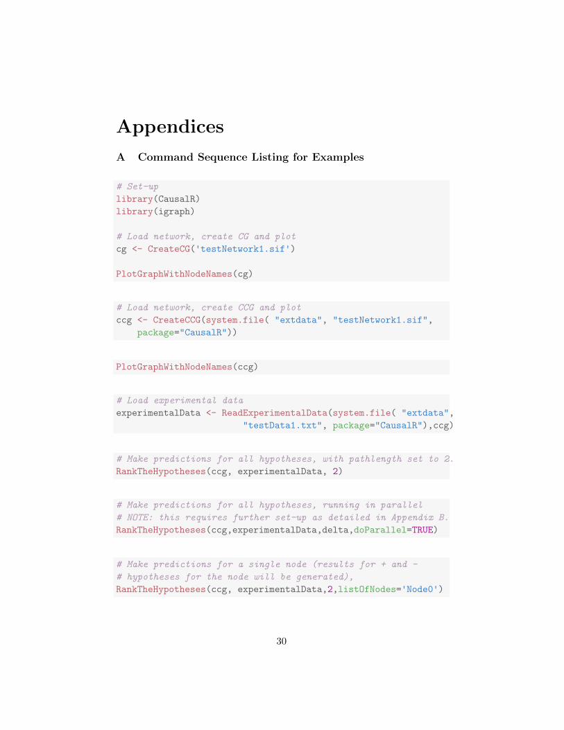
A Command Sequence Listing for Examples

# Set-up

library(CausalR)

library(igraph)

# Load network, create CG and plot

cg <- CreateCG('testNetwork1.sif')

PlotGraphWithNodeNames(cg)

# Load network, create CCG and plot

ccg <- CreateCCG(system.file( "extdata", "testNetwork1.sif",

package="CausalR"))

PlotGraphWithNodeNames(ccg)

# Load experimental data

experimentalData <- ReadExperimentalData(system.file( "extdata",

"testData1.txt", package="CausalR"),ccg)

# Make predictions for all hypotheses, with pathlength set to 2.

RankTheHypotheses(ccg, experimentalData, 2)

# Make predictions for all hypotheses, running in parallel

# NOTE: this requires further set-up as detailed in Appendix B.

RankTheHypotheses(ccg,experimentalData,delta,doParallel=TRUE)

# Make predictions for a single node (results for + and -

# hypotheses for the node will be generated),

RankTheHypotheses(ccg, experimentalData,2,listOfNodes='Node0')

30

# Make predictions for an arbitrary list of nodes (gives results

# for up- and down-regulated hypotheses for each named node),

testlist <- c('Node0','Node3','Node2')

RankTheHypotheses(ccg, experimentalData,2,listOfNodes=testlist)

# An example of making predictions for a particular signed hypo-

# -thesis at delta=2, for up-regulated node0, i.e.node0+.

# (shown to help understanding of hidden functionality)

predictions<-MakePredictionsFromCCG('Node0',+1,ccg,2)

GetNodeName(ccg,CompareHypothesis(predictions,experimentalData))

# Scoring the hypothesis predictions

ScoreHypothesis(predictions,experimentalData)

# Compute statistics required for Calculating Significance

# p-value

Score<-ScoreHypothesis(predictions,experimentalData)

CalculateSignificance(Score, predictions, experimentalData)

PreexperimentalDataStats <-

GetNumberOfPositiveAndNegativeEntries(experimentalData)

#this gives integer values for n_+ and n_- for the

#experimental data,as shown in Table 2.

PreexperimentalDataStats

# add required value for n_0, number of non-differential

# experimental results,

experimentalDataStats<-c(PreexperimentalDataStats,1)

# then use,

AnalysePredictionsList(predictions,8)

# ...to output integer values q_+, q_- and q_0 for

# significance calculations (see Table 2)

# then store this in the workspace for later use,

predictionListStats<-AnalysePredictionsList(predictions,8)

31

# Compute Significance p-value using default cubic algorithm

CalculateSignificance(Score,predictionListStats,

experimentalDataStats, useCubicAlgorithm=TRUE)

# or simply,


experimentalDataStats)

# as use cubic algorithm is the default setting.

# Compute Significance p-value using default quartic algorithm


experimentalDataStats,useCubicAlgorithm=FALSE)

# Compute enrichment p-value

CalculateEnrichmentPvalue(predictions, experimentalData)

# Running SCAN whilst excluding scoring of hypotheses for non-

# -differential nodes

AllData<-read.table(file="testData1.txt", sep="\t")DifferentialData<-AllData[AllData[,2]!=0,]

write.table(DifferentialData, file="DifferentialData.txt",

sep="\t",row.names=FALSE, col.names=FALSE, quote=FALSE )

runSCANR(ccg, ReadExperimentalData("DifferentialData.txt", ccg),

NumberOfDeltaToScan=3, topNumGenes=100,


# Indirect Individual Hypothesis Network Generation (after running SCAN)

WriteExplainedNodesToSifFile("Node1", +1,ccg,experimentalData,delta=2)

# Indirect Network Generation for All Hypotheses (after running SCAN)

scanResults <- runSCANR(ccg, experimentalData, numberOfDeltaToScan=2,

topNumGenes=4,correctPredictionsThreshold=1,

writeResultFiles = FALSE, writeNetworkFiles = "none",quiet=FALSE)

WriteAllExplainedNodesToSifFile(scanResults, ccg, experimentalData,

delta=2, correctlyExplainedOnly = TRUE, quiet = TRUE)

32

# Direct Network Generation for All Hypotheses (whilst running SCAN)

runSCANR(ccg, experimentalData, numberOfDeltaToScan=2,

topNumGenes=4,correctPredictionsThreshold=1,quiet=TRUE,

writeResultFiles = TRUE, writeNetworkFiles = "correct")

33

B Speeding-up CausalR Processing

The runtimes for RankTheHypotheses() increase with the size of networkand experimental input. This can be offset via the use of parallelisationor the R (JIT) byte code compiler (no additional package installations areneeded to use these as they are integral to the latest versions of base R).Note that run times will not be improved for very small examples where thecost of setting-up paralleisation or JIT outweighs its benefit.

Parallelisation is recommended for architectures featuring a multicore pro-cessor(s), whilst JIT is advised for older single or dual core machines.

Running RankTheHypotheses() in parallel :

Parallel processing can be activated via the doParallel flag,

RankTheHypotheses(ccg,experimentalData,delta,doParallel=TRUE)

By default the function will attempt to detect the number of available pro-cesser cores and use all of them bar one.

Alternatively, the number of cores to use can be set directly via the numCoresflag,

RankTheHypotheses(ccg,experimentalData,delta,

doParallel=TRUE, numCores=3)

To get the number of processor cores on their system:

Linux users can use the lscpu or nproc -all commands. In the absence ofuser privileges for these, try grep processor /proc/cpuinfo. The Linuxtop command can be used to check existing CPU utilisation.

Windows users can open a DOS window and type,

WMIC CPU Get DeviceID,NumberOfCores,NumberOfLogicalProcessors

or WMIC CPU Get /Format:List can be used.

34

Alternatively, they can look in the ’CPU Usage History’ under the WindowsTask manager ’Performance’ tab.

Running RankTheHypotheses() with JIT compilation :

In order to activate the R byte code compiler functionality, R must be startedwith an additional flag command, R COMPILE PACKAGES=1. This canbe done from the Linux or Windows command line when invoking R.

Alternatively, prior to starting R from the desktop icon on a Windows ma-chine, place the R COMPILE PACKAGES=1 after the path to Rgui.exe inthe Target field, under the Shortcut tab of the R icon Properties (accessedby right mouse click on the R icon).

Upon starting R, from double clicking the icon, the commands to use priorto loading CausalR are:

library(compiler)

enableJIT=3

When set to greater than zero, enableJIT invokes Just-In-Time (JIT) com-pilation, whilst enableJIT = 0 disables it. JIT can also be enabled bystarting R with the environment variable R ENABLE JIT set to 1, 2 or 3,depending upon the level required. CausalR works with the level set to 3.

For further details see, http://www.inside-r.org/r-doc/compiler/compileor, alternatively, type ??compiler :: compile at the R command prompt topull up the relevant R help page.

The JIT compiler compiles the package the first time it is run. Therefore, inorder to achieve speed-up, the user needs to run a small CausalR exampleprior to running a very large one. JIT can also be used for medium sizedinputs where the user wishes to run the computationally-expensive exactp-value calculation algorithm.

Note: when running very large networks/input the memory available to Rmay need reconfiguration (this is explained in the R documentation, butone easy way is to start-up R with the command line flag, -max-mem-size=????M, where ???? is a value in KB such that 4000M = 4MB (this can

35

also be inserted in the Windows icon Target field, see above). Use of 64bitR is also recommended in order to be able to address sufficient memory.

36

Overview of Causal Reasoning with CausalR Hypothesis ...€¦ · Table 1 is an example of the...

Documents

Transcript of Overview of Causal Reasoning with CausalR Hypothesis ...€¦ · Table 1 is an example of the...