Overview of Bohmian Mechanics and its extensions

Hoi Wai LAI

September 24, 2020

Supervisor: Prof. J.J. Halliwell

Submitted in partial fulfilment of the requirements for the degree of Master of Science of

Imperial College London

1

Abstract

It is well known that Copenhagen interpretation of quantum mechanics poses con-

ceptual difficulties such as the measurement problem. Bohmian mechanics also known

as de-Broglie Bohm theory is one of the simplest alternatives which explains quantum

phenomena while avoiding these conceptual difficulties. The underlying idea of this

theory is particles guided by the wave function. Although this idea seems natural,

somehow this picture is ignored or even rejected by the majority of the physics com-

munity. In this dissertation, an overview of Bohmian mechanics and its extensions will

be presented.

2

Contents

1 Introduction 5

2 Classical Mechanics 8

2.1 Lagrangian Mechanics . . . . . . . . . . . . . . . . . . . . . . . . . . . . . . 9

2.2 Hamiltonian Mechanics . . . . . . . . . . . . . . . . . . . . . . . . . . . . . . 9

2.3 Hamilton-Jacobi equation . . . . . . . . . . . . . . . . . . . . . . . . . . . . 10

2.3.1 Example - free particle . . . . . . . . . . . . . . . . . . . . . . . . . . 11

3 Bohmian Mechanics 13

3.1 Bohmian mechanics for spinless particles . . . . . . . . . . . . . . . . . . . . 13

3.2 Orthodox and Bohmian description of Double-slit experiment . . . . . . . . 16

3.3 Spin in Bohmian mechanics . . . . . . . . . . . . . . . . . . . . . . . . . . . 18

3.4 Conditional and effective wave function . . . . . . . . . . . . . . . . . . . . . 19

3.5 Stationary states . . . . . . . . . . . . . . . . . . . . . . . . . . . . . . . . . 21

3.6 Choice of beables . . . . . . . . . . . . . . . . . . . . . . . . . . . . . . . . . 22

4 Measurement theory of Bohmian Mechanics 23

5 Criticisms of Bohmian Mechanics and some responds 29

5.1 Criticisms . . . . . . . . . . . . . . . . . . . . . . . . . . . . . . . . . . . . . 29

5.2 Responds . . . . . . . . . . . . . . . . . . . . . . . . . . . . . . . . . . . . . 30

6 Making Bohmian Mechanics relativistic 33

6.1 A few ways to define simultaneity . . . . . . . . . . . . . . . . . . . . . . . . 34

6.1.1 Past and Future lightcone . . . . . . . . . . . . . . . . . . . . . . . . 34

6.1.2 Time foliation . . . . . . . . . . . . . . . . . . . . . . . . . . . . . . . 35

6.2 Synchronised trajectories . . . . . . . . . . . . . . . . . . . . . . . . . . . . . 37

7 Bohmian Mechanics and QFT 40

7.1 Schrodinger Field . . . . . . . . . . . . . . . . . . . . . . . . . . . . . . . . . 40

3

7.2 Electromagnetic Field . . . . . . . . . . . . . . . . . . . . . . . . . . . . . . 43

7.3 Problems of field ontology . . . . . . . . . . . . . . . . . . . . . . . . . . . . 46

7.4 Bell-type quantum field theories . . . . . . . . . . . . . . . . . . . . . . . . . 49

8 Conclusion 51

4

1 Introduction

In spite of the immense success of Newtonian physics on predicting the motion of macroscopic

objects from falling of an apple to the orbit of the moon, experiments such as the double

slit experiment, discovery of phenomena like black-body radiation and photoelectric effect

between the late nineteenth and early twentieth century forced us to abandon the Newtonian

description for the macroscopic world and opt for a more fundamental theory. At that time,

new physics was needed.

In 1905, Einstein in his Nobel prize winning paper postulated that light, which was thought

to be a wave, actually contains discrete energy quanta that we nowadays refer as photons in

order to explain the photoelectric effect. This revolutionised the classical view on continuous

entities like wave. The situation is similar to that on the first sight ocean waves seem to be

continuous, but a deeper investigation shows that it is an effect of a enormous number of

water molecules moving in a coherent way. Hence, the motion of the wave stems from motion

of water molecules. Furthermore in 1926, de Broglie proposed the idea of matter wave stating

that particles such as electrons and protons can display wave like behaviour. These ideas

were then generalised by Max Born, Werner Heisenberg and Erwin Schrodinger separately

to develop Matrix mechanics and wave mechanics respectively around 1925 which are the

earliest version of nowadays quantum mechanics and proved their equivalence by Dirac in

later years.

On the one hand, when a particle is observed, it always appears as a localised entity. On

the other hand, it acts as if it is a wave when no observation is involved. An interpretation

of quantum mechanics was needed in order to reconcile the properties. In the early devel-

opment of quantum mechanics, a few interpretations such as pilot-wave by de Broglie and

Copenhagen by Max Born and Werner Heisenberg were proposed. The most widely accepted

interpretation is the Copenhagen interpretation due to its simplicity as one only needs to

5

solve the Schrodinger equation (17) and accept a few axioms to predict the results of an

experiment. And to this day it is the most taught interpretation of quantum mechanics in

universities and standard quantum mechanics textbooks.

Over the years, there are many objections of the Copenhagen interpretation. The main prob-

lem is usually referred as the measurement problem which will be explained in section (4).

In short, Copenhagen interpretation not only has two dynamical rules which makes mea-

surements somewhat special, but also to a certain degree implies subjective reality. Another

minor problem is the superposition of states which was one of the problems that concerned

Bohm. The superposition of states comes from the fact that the Schrodinger equation is

linear. And based on that it is postulated that these states constitute a Hilbert space. If

one assumes that the Schrodinger equation is only an approximation of a more fundamental

equation which might involve a nonlinear term, then the construction of the Hilbert space is

no longer valid and thus the operator description of measurements fails. Another less imme-

diate problem is that the Copenhagen interpretation does not seem to give a clear ontology

to quantum theory. This problem is usual ignored by majority of the scientists. As long

as the predictions of the theory is consistent with experiments, why one should be bothered

with problems like this. However, in my opinion physics is not just experiments. Experi-

ments are just one of the many ways to ’test’ the world. Therefore, this interpretation is

closed to questions like what is objectively happening when measurement is not involved.

The best answer one could get is that there is nothing since we cannot see or measure the

wave function.

During the years, many other interpretations have been proposed as a solution to this prob-

lem. For example the many-worlds interpretation by Everett [19] which does not involve

collapse of the wave function, but branching of realities, the Ghirardi–Rimini–Weber theory

(GRW) [20] which involves spontaneous collapse and Bohmian Mechanics [6], [7] (a.k.a pilot-

wave theory or de Broglie Bohm theory) which introduces particles position as additional

6

variable and thus maintains a realistic view on the quantum world.

The idea of particles guided by wave was first proposed by de Broglie in the early development

of qunatum mechanics, but was abandoned due to the majority support of the Copenhagen

interpretation. It is then rediscovered by Bohm in 1952. And in the paper [7], Bohm showed

how the quantized electromagnetic field is described in this interpretation. This was the

earliest extension of Bohmian mechanics to field theory. At that time the theory was not

widely accepted by the scientific community because of political reasons. However, to Bell

the pilot wave interpretation seems so natural as stated in his article [5]

But why then had Born not told me of this ’pilot wave’? If only to point out

what was wrong with it? ... Why is the pilot wave picture ignored in text books?

Should it not be taught, not as the only way, but as an antidote to the prevailing

complacency? To show that vagueness, subjectivity, and indeterminism, are not

forced on us by experimental facts, but by deliberate theoretical choice?

It further inspired Bell to question the existence of local hidden-variable in quantum theory

in later year which then led to one of the most fundamental theorem of quantum theory, the

Bell’s theorem [3]. Bell then extended Bohmian mechanics to include spin [4] and developed

a version of Bohmian mechanics which contains creation and annihilation of particles [2].

In this dissertation, an overview of Bohmian mechanics and its extensions will be presented.

The organisation of this dissetation is as follows. In section (2), classical mechanics in its

different forms will be briefly discussed. In section (3), Bohmian mechanics will be intoduced

with some examples. Then the measurement theory of Bohmian mechanics will be analysed

in section (4). Then followed by a discussion of the criticisms of Bohmian mechanics. The

two remaining sections (6) and (7) will focus on the extensions of Bohmian mechanics related

to special relativity and quantum field theory respectively.

7

2 Classical Mechanics

It is believed that quantum mechanics is a more fundamental theory of reality. Therefore,

classical mechanics should be from quantum mechanics in certain limit. Namely, when ~

tends to zero (see [1] for a more detail analysis of how classical mechanics is recovered in

Bohmian mechanics). Thus, before going in to quantum mechanics, we first briefly explore

different formalisms of classical mechanics. Also, some of the ideas will be needed when a

Bohmian field theory is discussed in later sections. For simplicity, we only consider time-

independent Lagrangian and Hamiltonian.

Consider a system of N particles under a potential V , instead of working with N points

[~x1, ..., ~xN ] in real space, R3, one introduces configuration space Q ≡ R3N , whose coordinates

are q ≡ (~x1, ..., ~xN) for mathematical convenience. Then given two points qi and qf in

configuration space and travel time t = tf − ti. There is an infinite number of smooth paths

connecting these two points. Then the action S, a map from the space of all possible smooth

paths to the space of real number, is defined as follow.

S[q(t)] =

∫ tf

ti

L(q(t)), ˙q(t))dt (1)

where L(q(t)), ˙q(t)) = T − V is the Lagrangian of the system.

The actual path of the point in configuration space has to satisfies the principle of least

action. Mathematically, it is

δS = 0 (2)

In the following, three formulations of classical mechanics will be presented.

8

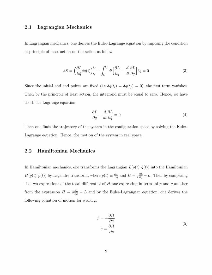
2.1 Lagrangian Mechanics

In Lagrangian mechanics, one derives the Euler-Lagrange equation by imposing the condition

of principle of least action on the action as follow

δS =(∂L∂qδq(t)

)tfti−∫ tf

ti

dt[∂L∂q− d

dt

∂L

∂q

]δq = 0 (3)

Since the initial and end points are fixed (i.e δq(ti) = δq(tf ) = 0), the first term vanishes.

Then by the principle of least action, the integrand must be equal to zero. Hence, we have

the Euler-Lagrange equation.

∂L

∂q− d

dt

∂L

∂q= 0 (4)

Then one finds the trajectory of the system in the configuration space by solving the Euler-

Lagrange equation. Hence, the motion of the system in real space.

2.2 Hamiltonian Mechanics

In Hamiltonian mechanics, one transforms the Lagrangian L(q(t), q(t)) into the Hamiltonian

H(q(t), p(t)) by Legendre transform, where p(t) ≡ ∂L∂q

and H = q ∂L∂q−L. Then by comparing

the two expressions of the total differential of H one expressing in terms of p and q another

from the expression H = q ∂L∂q− L and by the Euler-Lagrangian equation, one derives the

following equation of motion for q and p.

p = −∂H∂q

q =∂H

∂p

(5)

9

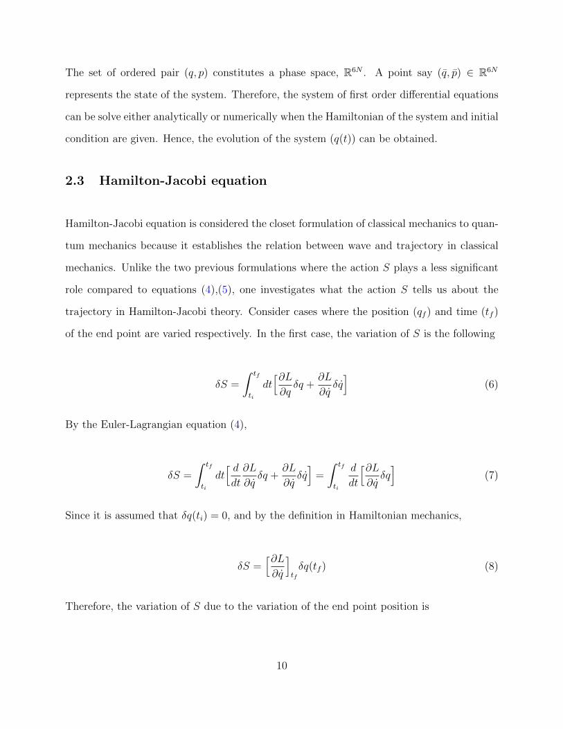
The set of ordered pair (q, p) constitutes a phase space, R6N . A point say (q, p) ∈ R6N

represents the state of the system. Therefore, the system of first order differential equations

can be solve either analytically or numerically when the Hamiltonian of the system and initial

condition are given. Hence, the evolution of the system (q(t)) can be obtained.

2.3 Hamilton-Jacobi equation

Hamilton-Jacobi equation is considered the closet formulation of classical mechanics to quan-

tum mechanics because it establishes the relation between wave and trajectory in classical

mechanics. Unlike the two previous formulations where the action S plays a less significant

role compared to equations (4),(5), one investigates what the action S tells us about the

trajectory in Hamilton-Jacobi theory. Consider cases where the position (qf ) and time (tf )

of the end point are varied respectively. In the first case, the variation of S is the following

δS =

∫ tf

ti

dt[∂L∂qδq +

∂L

∂qδq]

(6)

By the Euler-Lagrangian equation (4),

δS =

∫ tf

ti

dt[ ddt

∂L

∂qδq +

∂L

∂qδq]

=

∫ tf

ti

d

dt

[∂L∂qδq]

(7)

Since it is assumed that δq(ti) = 0, and by the definition in Hamiltonian mechanics,

δS =[∂L∂q

]tfδq(tf ) (8)

Therefore, the variation of S due to the variation of the end point position is

10

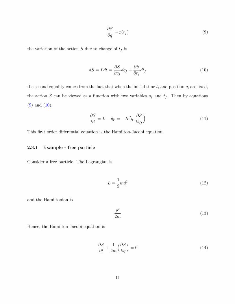
∂S

∂q= p(tf ) (9)

the variation of the action S due to change of tf is

dS = Ldt =∂S

∂qfdqf +

∂S

∂tfdtf (10)

the second equality comes from the fact that when the initial time ti and position qi are fixed,

the action S can be viewed as a function with two variables qf and tf . Then by equations

(9) and (10),

∂S

∂t= L− qp = −H

(q,∂S

∂qf

)(11)

This first order differential equation is the Hamilton-Jacobi equation.

2.3.1 Example - free particle

Consider a free particle. The Lagrangian is

L =1

2mq2 (12)

and the Hamiltonian is

p2

2m(13)

Hence, the Hamilton-Jacobi equation is

∂S

∂t+

1

2m

(∂S∂q

)= 0 (14)

11

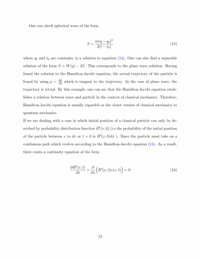
One can check spherical wave of the form

S =m(q − q0)2

2(t− t0)(15)

where q0 and t0 are constants, is a solution to equation (14). One can also find a separable

solution of the form S = W (q) − Et. This corresponds to the plane wave solution. Having

found the solution to the Hamilton-Jacobi equation, the actual trajectory of the particle is

found by using p = ∂S∂q

which is tangent to the trajectory. In the case of plane wave, the

trajectory is trivial. By this example, one can see that the Hamilton-Jacobi equation estab-

lishes a relation between wave and particle in the context of classical mechanics. Therefore,

Hamilton-Jacobi equation is usually regarded as the closet version of classical mechanics to

quantum mechanics.

If we are dealing with a case in which initial position of a classical particle can only be de-

scribed by probability distribution function R2(x, 0) (i.e the probability of the initial position

of the particle between x to dx at t = 0 is R2(x, 0)dx ). Since the particle must take on a

continuous path which evolves according to the Hamilton-Jacobi equation (11). As a result,

there exists a continuity equation of the form

∂R2(x, t)

∂t+

∂

∂x

(R2(x, t)v(x, t)

)= 0 (16)

12

3 Bohmian Mechanics

3.1 Bohmian mechanics for spinless particles

In Bohmian Mechanics, the complete description of a system is given by the wave function

ψ and its configuration Q. The wave function ψ(q, t) evolves according to the Schrodinger

equation in position representation (17), where q = (~x1, ..., ~xN). The evolution of the config-

uration is determined by the guiding equation (18) which can be regarded as a consequence

of the Schrodinger equation. Bohmian mechanics is said to be deterministic because once

the initial state of the system (ψ(q, 0), Q(0)) is given, the dynamics of the state is uniquely

determined for all future time by equations (17) and (18). Unlike orthodox quantum me-

chanics where there are two sets of dynamical rules, these two equations account for all the

quantum phenomena involving spinless particles.

Consider a single spinless particles under the potential V , the Schrodinger equation is

i~∂ψ(~x, t)

∂t=−~2

2m∇2ψ(~x, t) + V (~x, t)ψ(~x, t) (17)

and the guiding equation is

d ~X(t)

dt=

J(~x, t)

|ψ(~x, t)|2

∣∣∣∣∣~x= ~X(t)

=~m

Im(ψ∗∇ψ|ψ|2

)∣∣∣∣∣~x= ~X(t)

(18)

where J(~x, t) is the probability current density. Generalisation to many-particles is trivial in

which ~x is replaced by q = (~x1, ..., ~xN) and the configuration X by Q. The second expression

of equation (18) seems redundant as there is common factor of ψ∗ in the numerator and

denominator. However, the advantage of this expression is that it provides a easy transition

to particles with spin.

13

The probability current density J(~x, t) comes from the associated continuity equation to the

Schrodinger equation. By multiplying ψ and its complex conjugate ψ∗ respectively on the

Schrodinger equation and its complex conjugation. One has

ψ∗i~∂ψ

∂t= −ψ∗ ~

2

2m∇2ψ + ψ∗V ψ

−ψi~∂ψ∗

∂t= −ψ ~2

2m∇2ψ∗ + ψ∗V ψ

(19)

Then subtracting one off the other, one gets

∂|ψ|2

∂t= i

~2m∇(ψ∗∇ψ − ψ∇ψ∗

)(20)

usually it is written in a more compact form of

∂ρ

∂t+∂J

∂x= 0 (21)

where ρ = ψ∗ψ = |ψ|2 and J = ~2im

(ψ∗∇ψ − ψ∇ψ∗

).

To see where the guiding equation comes from, we follow Bohm’s paper [6] in 1952. Firstly,

put the wave function ψ in polar form ψ = ReiS~ then substituting it into the Schrodinger

equation (17). The imaginary and real part then are,

∂R

∂t= − 1

2m

[R∇2S + 2∇R∇S

](22)

∂S

∂t= −

[(∇S)2

2m+ V (x)− ~2

2m

∇2R

R

](23)

14

By comparing equation (23) and the Hamilton-Jacobi equation (11), then the natural in-

terpretation of the phase S is to regard it as the quantum action. Unlike the classical

Hamilton-Jacobi equation, there is an extra term Q(x, t) ≡ − ~22m∇2RR

called the quantum

potential. Equation (23) is commonly regarded as the quantum Hamilton-Jacobi equation.

Rewriting R =√ρ, equation (22) then implies

∂ρ

∂t+∇

(ρ∇Sm

)=∂R2

∂t+∇

(R2∇S

m

)= 0 (24)

By comparing this to the continuity equation (16) of a particle with uncertain initial position

in the classical case, it is natural to define the Bohmian velocity as

v =J(x, t)

ρ=∇Sm

(25)

it can be shown that the two expressions are equivalent to the previous expression. As a result,

the guiding equation is merely a consequence of the Schrodinger equation. One then interprets

|ψ(x, t)|2dx as the probability of the particle at position x. Or equivalently, if a system

has wave function ψ(q, t), then its configuration Q is random with probability distribution

|ψ(q, t)|2. This is referred as the quantum equilibrium hypothesis. The justification of this

is a delicate matter and is beyond the scope of this dissertation. A detailed argument of

this is given in [11] by Durr, Goldstein and Zanghi in which typicality and the law of large

number in probability theory are used for the argument. In addition, if at initial time the

distribution is |ψ(x, 0)|2, then at later time the distribution is |ψ(x, t)|2. This property is

called equivariance. Since |ψ(x, t)|2 acts as R2(x, t) in equation (16), the initial position of

the particle cannot be known with certainty, but when the experiment is ran for many times

|ψ(x, t)|2 should be reproduced.

In Bohm’s paper, he then formulated this theory in terms of force like Newton’s equation.

15

Hence, one can simply treat a quantum system like a classical system but with an additional

’quantum’ force coming from the quantum potential Q. Even though this way of looking at

Bohmian Mechanics gives us some insights on how quantum phenomenons work when the

word ’particle’ is taken in the literal sense, it is like putting quantum mechanics in a classical

mould.

After all Bohmian mechanics is a first order theory unlike Newton’ equation which is second

order. Hence, a more common view of equation (17) and (18) is to interpret and treat

the wave function ψ like the Hamiltonian H(q, p) in Hamiltonian formulation of classical

mechanics in which the Hamiltonian generates a vector field in phase space and the evolution

of the system is the integral curve of the field. In Bohmian mechanics, the wave function

ψ generates a vector field in configuration space. Hence, the evolution of the system is the

integral curve of the vector field.

3.2 Orthodox and Bohmian description of Double-slit experiment

In the double slit experiment, electrons are fired toward the slits one at a time and its posi-

tion is registered by a screen in the opposite side of the source. After firing a large number

of electrons, an interference pattern is observed. This suggests that the underlying theory

determining the motion of electrons cannot be classical mechanics, but quantum mechanics.

In standard quantum mechanics, by the principle of complementarity, a physical object dis-

plays its wave or particle property depending on the type of measurement. In the case of the

double slit experiment, before going through the slits, an electron is represented by a plane

wave. When the plane wave hits the slits, it creates two circular wave sources and hence

an interference pattern. By Bohr’s rule, the probability of finding the electron within x to

x+ dx of the screen is |ψ(x, t)|2dx. When an electron is detected, it is said to be showing its

particle-like property.

16

With this interpretation, questions such as, what is the position of the electron before it

hits the screen, and more fundamentally what is an electron, can be very confusing or even

cannot be answered. Therefore, it is unclear how this interpretation gives us an image of the

world.

In contrast, Bohmian mechanics maintains the view that a particle is a particle. By quantum

equilibrium hypothesis, the initial position of the electron cannot be known with certainty

and can only be described by |ψ(x, 0)|2 due to the lack of knowledge. Then by the property

of equivariance, at a later time the probability of the electron at x is |ψ(x, t)|2. During the

process the wave function ψ(x, t) is only responsible for guiding the electron which has a

continuous trajectory all along. In other word, the particle goes through one and only one

of the slits while the wave function acts as ordinary wave which passes both slits and guides

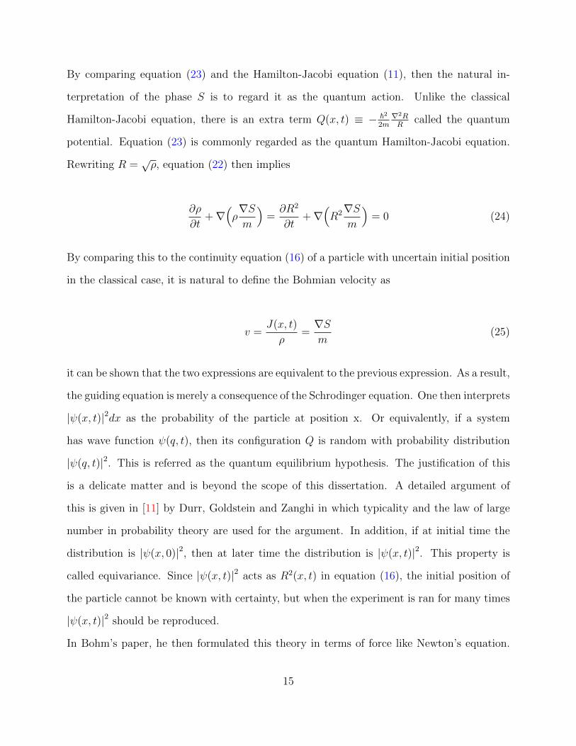
the particle. A figure of possible Bohmian trajectories (1) is shown at end of this section.

Problems that stated above regrading the Copenhagen interpretation do not exist in Bohmian

mechanics. For example, the answer of the question of what is an electron is simple. An

electron is a particle in the literal sense and it is represented by a point mathematically just

like any other particles in classical mechanics. Since there is no electromagnetic field in the

experiment, spin is not accounted for. Unlike Copenhagen interpretation, the image of a

Bohmian universe is quite clear in which the fundamental physical entities are particles and

their positions.

In [26], researchers reconstructed the trajectories of an ensemble of photons in a double slit

experiment using weak measurement. The resulting trajectories of photons resemble that of

the Bohmian trajectories.

17

Figure 1: regions that have a high density of trajectories correspond to the bright fringes onthe screen and vice versa for dark fringes. Figure from [17] based on [33]

.

3.3 Spin in Bohmian mechanics

In standard quantum mechanics, spin is regarded as an intrinsic property of a particle in

which there is no classical analogue. Therefore, it seems like additional variables are needed

to account for every degree of spin freedom. In Bohmian mechanics, even though one can

indeed introduce additional variables for spin, this tends to complicate the mathematics.

However, Bell [4] showed us that spin can be treated as a property of the wave function

instead of the particle’s. For simplicity we will only discuss the case s = 12. For a spin half

particle, its wave function is a spinor wave function,

~ψ(~x, t) =

ψ 12(~x, t)

ψ− 12(~x, t)

(26)

18

which is a map R3+1 7−→ C2. And the evolution of this wave function given by the Pauli

equation (27) instead of the Schrodinger equation (17),

i~∂ ~ψ(~x, t)

∂t=[ 1

2m~σ(−i~∇− q ~A(~x, t))2 + V

]~ψ(~x, t) (27)

where ~σ are the Pauli matrices and ~A(~x, t)) is the vector potential. Then one can define the

Bohmian velocity in a similar way as for spinless particles case.

~v(~x, t) =~J(~x, t)

ρ(~x, t)(28)

where ρ = ~ψ† · ~ψ and ~J is the probability current of the Pauli equation (27).

These two equations (27) and (28) together account for every phenomena involving spin.

Unlike standard quantum mechanics, spin is not considered as an intrinsic property of a

particle, but a property of the wave function and will affect the trajectory of a particle via

the guiding equation (28). This is shown by the fact that the wave function is a function

of only position and time. Also. there is no guiding equation for spin components of the

particles. A detailed formulation of Bohmian mechanics involving spin can be found in [30].

3.4 Conditional and effective wave function

Before going into the how measurement is described in Bohmian mechanics. We discuss some

physical implications of Bohmian mechanics. In a universe governed by Bohmian mechanics,

because the theory is deterministic and the velocity of a particle depends on the instantaneous

position of all other particles, there is a sense of ’wholeness’ in which one is lead to the

concept of wave function of the universe Ψ(u). An immediate question is that assuming

the wave function of the universe Ψ(u) and its configuration Q(t) evolves according to the

19

Schrodinger equation and the guiding equation respectively, why the subsystems which we

deal with in a laboratory seem to follow the Schrodinger equation and guiding equation of the

subsystem instead of being influenced by its environment. This then leads us to the concept

of conditional wave function and effective wave function.

Consider the following, in a universe with N particles with configuration Q and wave function

Ψ(u)(q, t). The wave function of the universe follows the many-particle Schrodinger equation

i~∂Ψ(u)(q)

∂t=

N∑i=1

− ~2

2mi

∂2Ψ(u)(q, t)

∂qi2+ V (q, t)Ψ(u)(q, t) (29)

while its configuration evolves according to guiding equation

dQ

dt=

J(q, t)

|Ψ(u)(q, t)|2

∣∣∣∣∣q=Q(t)

(30)

Say we are interested on a subset of the particles, a subsystem with M < N particles whose

configuration is X. Hence, the configuration of the universe is given by Q = (X, Y ) where

Y is the configuration of the environment of the subsystem. Then we define the conditional

wave function of the subsystem by

φ(x) = Ψ(u)(x, Y, t) (31)

In general, the conditional wave function (31) is not governed by the Schrodinger equation

but a more complicated equation. However, if the wave function of the universe Ψ(u) is of

the form

Ψ(u)(x, y, t) = φ(x, t)α(y, t) + Ψ⊥(x, y, t) (32)

20

where α(y, t) and Ψ⊥(x, y, t) do not overlap in y configuration space. In other word, they

have disjoint macroscopic supports. If the configuration Y is in the support of α(y, t), then

we define φ(x, t) as the effective wave function. And φ(x, t) will evolve according to the

Schrodinger equation of the subsystem. This usually happens after a quantum measurement

which will be discussed in section (4). A point to note is that effective wave function of a

subsystem does not necessarily exist since the situation above does not always happen. But

if it does exist, then it will be proportional to the conditional wave function which can be

seen by comparing equation (31) and (32). In the rest of the paper, the wave function of the

system will be the effective wave function.

3.5 Stationary states

In this interpretation, there is an interesting phenomena about a special type of stationary

states. Just like standard quantum mechanics, stationary wave functions are the separable

solutions to the Schrodinger equation (17) of the form φ(~x)e−iEt~ . Putting it into the following

form

ψ(~x, t) = R(~x)exp[i(α(~x)− Et)

~

](33)

the phase of the wave function is S = α(~x) − Et. Then by ~v = 1m∇S, one can see the if

∇S = ∂α(~x)∂~x

= 0, the position of the particle is constant. Hence, the particle appears to

be stationary. However, this does not mean there is only one result when one measures the

position of the particle. Because of the quantum equilibrium hypothesis, the distribution of

position result will be |ψ(~x, t)|2. Electron in the s = 0 state in a hydrogen atom is one of the

example that exhibits this behaviour. In fact, any system with a spherical symmetric wave

function or real wave function will exhibit this behaviour.

Consider a free particle, the Schrodinger equation is

21

i~∂ψ(~x, t)

∂t=−~2

2m∇2ψ(~x, t) (34)

then plane wave of the form ψ(~x, t) ∝ exp[i (~p·~x−Et)~ ]. By ∇S = ∂α(~x)

∂~x= ~p. Hence, the velocity

of the particle is constant and the trajectory of it is a straight line as in the example in

section (2). More examples and detail analysis of stationary states can be found in [6].

3.6 Choice of beables

In Bohmaian mechanics, we exclusively use the position representation of the Schrodinger

equation. And the position of the particles as an addition ’hidden variable’or beable. How-

ever, in standard quantum mechanics one can use any representation of the Schrodinger

equation. Therefore, one would question if it is possible to construct a Bohmian-type theory

in which beable other than position, such as momentum, is used. A beable in Bell sense is an

entity that exists in reality with or without observation. Also, it should give an image of the

physical world. Therefore, it is a question of ontology of theory and whether it is consistent

with the image of the world that we observe. In fact, additional to the position of particles,

one can include other beable and this has been done by Holland [24]. See [18] for a detailed

discussion regarding the ontology of Bohmian mechanics.

22

4 Measurement theory of Bohmian Mechanics

One of the most criticised issue of the orthodox quantum mechanics is its conceptual difficulty

regarding measurements. It is usually referred as the measurement problem. In Bohmian

mechanics, this problem does not exist since there is only one dynamical rule. Therefore,

before analysing the measurement theory of Bohmian mechanics. A brief discussion of the

measurement theory of Orthodox quantum mechanics is needed.

Firstly, in standard quantum mechanics the wave function ψ itself provides a complete de-

scription of the system. Secondly, the evolution of wave function is continuous and deter-

ministic according to the Schrodinger equation in cases where measurement is not involved.

Thirdly, upon measurement the wave function ’collapses’ to one of the eigenstates of the

corresponding operator. Mathematically, an observable A is associated with a Hermitian

operator A whose eigenstates |ai〉 span the Hilbert space in which the state |ψ〉 lives in.

Therefore, |ψ〉 can be expressed in terms of those eigenstates as

|ψ〉 =N∑i

〈ai|ψ〉 |ai〉 =N∑i

ci |ai〉 (35)

where 〈ai|ψ〉 is the inner product in Hilbert space, in position representation it is 〈ai|ψ〉 =∫a∗i (x)ψ(x)dx. Also, non-degeneracy and discrete spectrum are assumed for simplicity. Then

the act of measurement is represented by operator acting on the state as

A |ψ〉 =N∑i

〈ai|ψ〉 ai |ai〉 (36)

where ai is the eigenvalue of the eigenstate |ai〉. The probability of getting the measurement

result of ai is |〈ai|ψ〉|2 with∑N

i |ci|2 = 1. For example if one measured the value a2, then the

state |ψ〉 is said to collapse to the eigenstate |a2〉. And for any subsequent measurement on

23

the system, one has to use the state |a2〉. This quantum phenomena is called collapse of the

wave function which is not accounted for by the Schrodinger equation in standard quantum

mechanics, but by the measurement axiom.

Even though standard quantum mechanics has a great success on predicting the results of

quantum measurements, it leaves some significant conceptual problems unanswered. First

of all, this interpretation puts measurement in a special place in the theory. And hence

unavoidably involves an observer. These leads to ambiguity on what a measurement is and

what qualifies to be an observer. Even great physicists like Richard Feynman once said

This is all very confusing, especially when we consider that even though we may

consistently consider ourselves to be the outside observer when we look at the

rest of the world, .... Does this then mean that my observations become real only

when I observe an observer observing something as it happens? This is a horrible

viewpoint. Do you seriously entertain the idea that without the observer there is

no reality? Which observer? Any observer? Is a fly an observer? ...

And hence there is no specification on which dynamical law should be used in which circum-

stances. Secondly, the fact that one uses an operator to represent the environment of the

system makes the separation of the system and its environment unclear.

In Bohmian Mechanics, the dynamics of a system is solely determined by the Schrodinger

equation (17) and guiding equation (18). Instead of having another set of dynamical rule

for measurement processes, one simply treats the interaction between the system and the

measurement apparatus, such as a pointer, like any other interaction between particles to

account for measurement processes. As a result, Bohmian mechanics is sometimes referred

as the ’quantum mechanics without observers’ since there is no involvement of an observer.

Also, one can show that not only operators naturally emerge from the analysis of a Bohmian

measurement, but also the measurement axiom in standard quantum mechanics is actually

a consequence of it. However, due to computational burden it is impossible to practically

24

calculate the evolution of the coupled system because a classical describable measurement

apparatus contains more than 1023 particles.

Even though the measurement theory of Bohmian mechanics gives the same results as the

orthodox quantum mechanics, the mathematics behind is quite different. To analysis a mea-

surement in Bohmian term, we follow a similar approach by [31] and [17].

Suppose the state of the system and pointer are (ψ(x, t), X) and (φ(y, t), Y ) respectively,

where X and Y are the actual configurations of the system and pointer. Then the total wave

function is Φ(x, y, t).

Assuming the pointer points at a discrete set of values so the value space is λ = [α1, α2, ..., αN ].

If the wave function of the system is ψα1 , then the pointer should point at the value α2 after

the measurement. We further assume that this value space is completed, meaning that all

possible wave functions are included. Also, since the pointer is a macroscopic object, φαi and

φαj should not overlap for i 6= j. Thus, they represent different macrostates. A measurement

apparatus that satisfies above conditions is referred as a good measurement device.

Before measurement by linearity, the wave function of the system is

ψ(x, t) =N∑i

ci(t)ψαi (37)

where we assume∑N

i |ci|2 = 1 for convenience. And the wave function of the pointer is φ0

where it is the support of the pointer pointing null direction. During the measurement, the

total wave function of the system plus pointer is in an entangled state

Φ(x, y, t) =N∑i

ci(t)ψαi(x)φαi(y, t) (38)

To get a unique result, the initial configuration of the system (X(0)) and pointer (Y (0))

are needed. During the measurement, the configuration of the total system (X(t), Y (t)) will

25

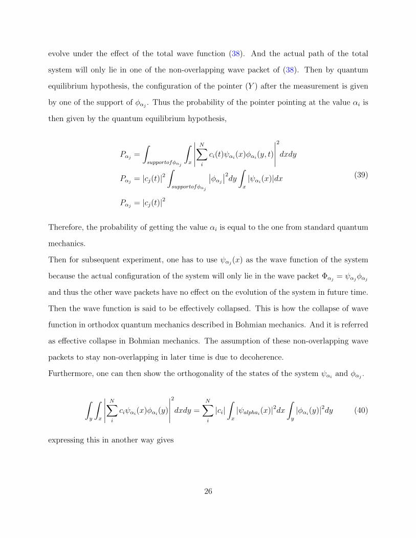
evolve under the effect of the total wave function (38). And the actual path of the total

system will only lie in one of the non-overlapping wave packet of (38). Then by quantum

equilibrium hypothesis, the configuration of the pointer (Y ) after the measurement is given

by one of the support of φαj . Thus the probability of the pointer pointing at the value αi is

then given by the quantum equilibrium hypothesis,

Pαj =

∫supportofφαj

∫x

∣∣∣∣∣N∑i

ci(t)ψαi(x)φαi(y, t)

∣∣∣∣∣2

dxdy

Pαj = |cj(t)|2∫supportofφαj

∣∣φαj ∣∣2dy ∫x

|ψαi(x)|dx

Pαj = |cj(t)|2

(39)

Therefore, the probability of getting the value αi is equal to the one from standard quantum

mechanics.

Then for subsequent experiment, one has to use ψαj(x) as the wave function of the system

because the actual configuration of the system will only lie in the wave packet Φαj = ψαjφαj

and thus the other wave packets have no effect on the evolution of the system in future time.

Then the wave function is said to be effectively collapsed. This is how the collapse of wave

function in orthodox quantum mechanics described in Bohmian mechanics. And it is referred

as effective collapse in Bohmian mechanics. The assumption of these non-overlapping wave

packets to stay non-overlapping in later time is due to decoherence.

Furthermore, one can then show the orthogonality of the states of the system ψαi and φαj .

∫y

∫x

∣∣∣∣∣N∑i

ciψαi(x)φαi(y)

∣∣∣∣∣2

dxdy =N∑i

|ci|∫x

|ψalphai(x)|2dx∫y

|φαi(y)|2dy (40)

expressing this in another way gives

26

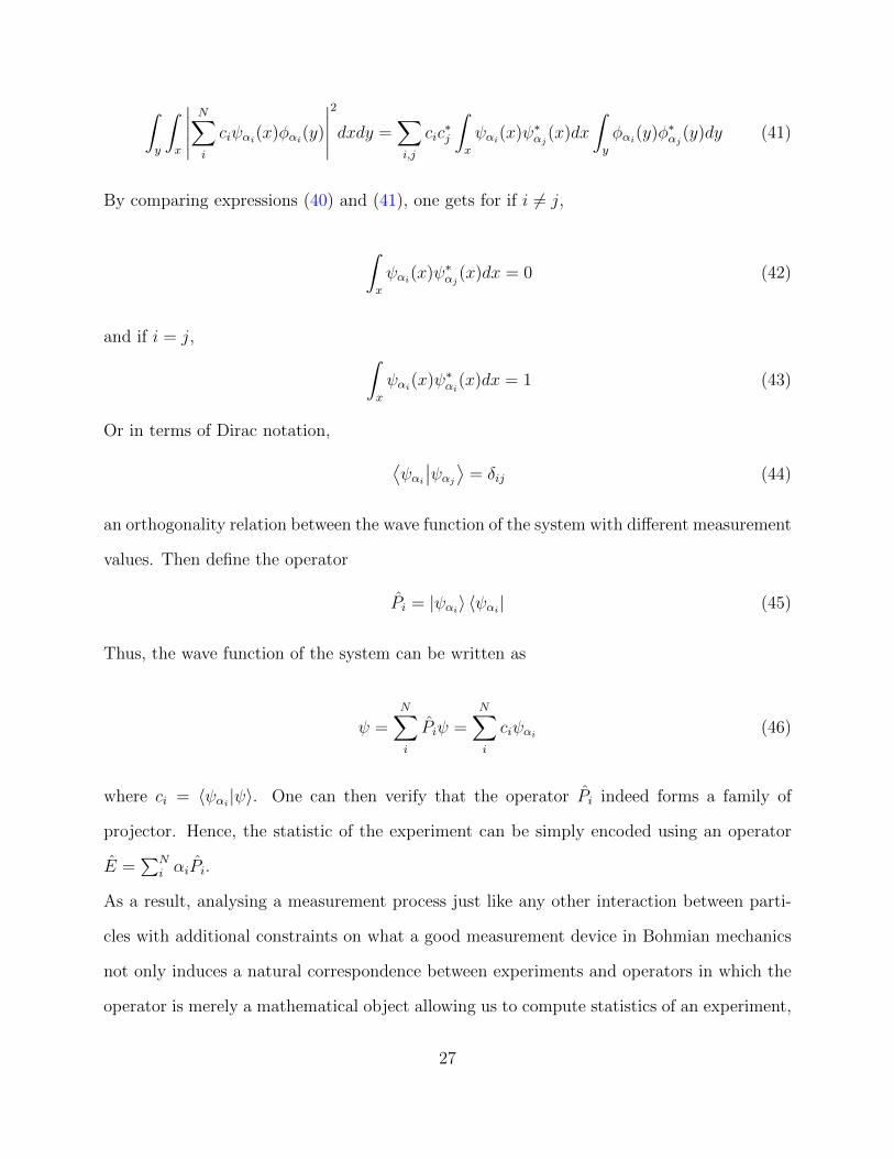
∫y

∫x

∣∣∣∣∣N∑i

ciψαi(x)φαi(y)

∣∣∣∣∣2

dxdy =∑i,j

cic∗j

∫x

ψαi(x)ψ∗αj(x)dx

∫y

φαi(y)φ∗αj(y)dy (41)

By comparing expressions (40) and (41), one gets for if i 6= j,

∫x

ψαi(x)ψ∗αj(x)dx = 0 (42)

and if i = j, ∫x

ψαi(x)ψ∗αi(x)dx = 1 (43)

Or in terms of Dirac notation, ⟨ψαi∣∣ψαj⟩ = δij (44)

an orthogonality relation between the wave function of the system with different measurement

values. Then define the operator

Pi = |ψαi〉 〈ψαi | (45)

Thus, the wave function of the system can be written as

ψ =N∑i

Piψ =N∑i

ciψαi (46)

where ci = 〈ψαi |ψ〉. One can then verify that the operator Pi indeed forms a family of

projector. Hence, the statistic of the experiment can be simply encoded using an operator

E =∑N

i αiPi.

As a result, analysing a measurement process just like any other interaction between parti-

cles with additional constraints on what a good measurement device in Bohmian mechanics

not only induces a natural correspondence between experiments and operators in which the

operator is merely a mathematical object allowing us to compute statistics of an experiment,

27

but also in fact defines a boarder class of allowed operators. This is called Positive-operator

valued measure (POVM). And in standard quantum mechanics, one usually promotes a clas-

sical observable to operator. This defines a projection-valued measure (PVM) which is a

special case of POVM. For a detail analysis of POVM in Bohmian see [17].

28

5 Criticisms of Bohmian Mechanics and some responds

5.1 Criticisms

Despite the fact that Bohmain mechanics gives the same predictions as standard quantum

mechanics, there are a lot of oppositions on whether it should be the correct model for our

universe. In this section, a few important ones will be discussed.

First of all, one of the most problematic issues of Bohmian mechanics is the explicit non-

locality of the theory which can be seen in equation (18), where the velocity of a particle is

under the influence of the instantaneous position of all other particles even they are spacelike

separated. This strictly violates the spirit of special relativity in which an event outside

the lightcone of another event cannot be causally related. This makes Bohmian mechanics

exceptionally hard to combine with special relativity. Also, some might quote Bell’s theorem

stating that Bell’s theorem ruled out all hidden-variable theory including Bohmian mechan-

ics.

Another problem of Bohmian mechanics is that it seems to violate the action-reaction prin-

ciple. In Bohmian mechanics, the wave function ψ acts as a guiding wave which generates a

time-dependent vector field in the configuration space. Hence, the configuration of the system

X is the integral curve of the vector field. However, there is no action from the configuration

X on the wave function ψ. This can be seen simply in the Schrodinger equation (17) as the

evolution of the wave function does not depend on the configuration.

Thirdly, as Bohm suggested one should interpret the wave function ψ like any other real

physical fields such as electromagnetic field. When one thinks of a physical field, for example

a scalar field, it defines a number at each point in space. However, the wave function defines a

number at each point in configuration space. Therefore, if wave function is to be regarded as

a physical field, then one must accept the fact that configuration space which was introduced

for mathematical convenience in classical mechanics is actually physical.

29

Another concern of Bohmian mechanics is that it seems to be impossible to develop is version

of Bohmian mechanics with particle creation and annihilation. Because position of particles

is a beable of the theory. Hence, a particle is an entity that exists with or without observa-

tion.However, this is not true. A version of Bohmian mechanics that incorporates creation

and annihilation of particle will be presented in section (7).

5.2 Responds

Regarding non-locality, Bell’s theorem (See [28] for a proof and brief discussion of Bell’s

theorem and its implication of hidden variable theory) is telling us that locality in Einstein

sense will always be violated by a theory that describes quantum phenomena in terms of

some local hidden variables. As a result, one can say that non-locality is a feature of the

universe. Therefore, Bohmian mechanics is not ruled out by Bell’s theorem because the

guiding equation is non-local. But Rather it brings out the explicit non-locality of the

universe. As Bell stated in his book [5]

That the guiding wave, in the general case, propagates not in ordinary three-

dimensional space but in a multidimensional configuration space is the origin

of the notorious “nonlocality” of quantum mechanics. It is a merit of the de

Broglie–Bohm version to bring this out so explicitly that it cannot be ignored.

Even though this explicit non-locality poses difficulties on combining Bohmian mechanics

with special relativity, there are a few versions of relativistic Bohmian mechanics that are

consistent with experimental results.

On the violation of action-reaction principle in classical mechanics by Bohmain mechanics,

since the action-reaction principle is essentially one of the consequences of the underlying

Galilean symmetry of theory, in Bohmian mechanics Galilean symmetry can be achieved

without imposing action from the configuration to the wave function. Therefore, action-

30

reaction principle is not violated, but is merely not a consequence of the theory for it to be

Galilean invariant. In addition, if one considers the conditional wave function of the system

(31), then the configuration of the environment of the subsystem does have an effect on the

wave function.

In [16], the authors argued that these problems of Bohmian mechanics stems from a more

fundamental question of what is the meaning of the wave function. A different view of the

wave function ψ is suggested in which essentially the wave function is not considered as a

real physical field as Bohm suggested. Instead, it should be regarded as an interpretation-less

nonphysical object that is one of the element of the theory and not an entity described by

the theory.

This is similar to the case of Hamiltonian in classical mechanics. Hamiltonian of a system

is a function of phase space which is equally or even more unphysical than the configuration

space. Since Hamiltonian is not considered as an physical entity described by the law, but

part of the law. Therefore, there is no argument saying that phase space is physically real.

Furthermore, the authors hypothesise that instead of the time-dependent Schrodinger equa-

tion (17), the time-independent Schrodinger equation (5.2)

HΨ(u) = EΨ(u) (47)

is the fundamental equation that governs the universe at least in the non-relativistic regime.

And the time-independent wave function of the universe Ψ(u) is responsible for generating a

vector field in the configuration space and thus guides the motion of Q. In this case, Q is

not the position of all the particles in the universe, but some abstract configurations. An

immediate question of such hypothesis is where does time-dependent Schrodinger equation

of the subsystem come from if the wave function of the system (i.e the universe) is time

independent. An simple example is shown and argued that this should also happen in a

31

more general situation.

This interpretation of the wave function eliminates the problem of physical configuration

space. However, if the wave function is no longer considered a physical entity, then the state

of a system is only given by its configuration Q. For example, in double slit experiment, the

wave function does not act as a guiding wave, a particle simply goes through one of slits and

its trajectory is described by the law. Therefore, it is unclear how the interference pattern

develops without invoking entity like a wave.

Actually, the problem of how the wave function should be interpreted and its meaning is

not only a question on the mathematical level, but also on a philosophical level. A further

discussion of the role of wave function in different interpretation of quantum mechanics and

other related philosophical problems see [18] and [23].

32

6 Making Bohmian Mechanics relativistic

As mentioned in the previous section, non-locality in guiding equation poses difficulties on

unifying Bohmian mechanics and special relativity. More precisely, since the velocity of one

particle depends on the instantaneous position of all other particles, one has to specific a

hypersurface or a reference frame to introduce simultaneity. It is believed that a relativistic

version of Bohmian mechanics cannot be developed without invoking structures like these.

In relativistic setting, time and position are treated on an equal footing. Hence, a natural

generalisation of the wave function of a N spinless particles system ψ(~x1, ..., ~xN , t), which is

a map from the space R3N+1 to C, is the multi-time wave function

ψ((t1, ~x1), ..., (tN , ~xN)) (48)

where ((t1, ~x1), ..., (tN , ~xN)) is referred as the spacetime configuration. Then the wave function

we use in quantum mechanics is just the special case of the multi-time wave function (48) in

which t1 = ... = tN . A detail analysis of the Multi-time wave function is given in [27]. In the

following, we assume the consistency condition is fulfilled.

In the case of a single particle, the wave equation and guiding equation are

Lψ(x) = 0 (49)

dXµ

dλ∝ jµ(x)

∣∣∣x=X(λ)

(50)

where L is a linear combination of of some differential operators defining the wave equation,

for example, for the Klein-Gordon equation L = ∂2 +m2. λ is the parameter of the curve Xµ.

These equations are Lorentz invariant. However, the guiding equation is no longer Lorentz

33

invariant if the system has N particles, then the guiding equation in such a case is,

dXµa (λa)

dλa∝ jµ(X1(λ1), ..., XN(λN)) (51)

Hence, one has to define at which point of X, j should be evaluated. The most naive way

to do this is to use a preferred reference frame. However, this method is clearly not Lorentz

invariant because different frame leads to different particle trajectories.

6.1 A few ways to define simultaneity

6.1.1 Past and Future lightcone

Since there is no issue on differentiating the temporal order of events that are timelike sep-

arated, all one has to do is to define simultaneity for spacelike separated events. Therefore,

instead of using a preferred reference frame, there are a few different proposals. One could

use either the future or past lightcone to define a simultaneous surface which was proposed

by Squires and Goldstein in [35] and [22] respectively. However, both methods have their

problems respectively. If one uses the past lightcone, then the resulting theory will be local.

Therefore, this theory cannot be a satisfactory one as Bell’s theorem demands non-locality.

On the other hand, if one uses the future lightcome, then the resulting theory is in fact non-

local, but it does not has an equivariant measure. Although as shown in next subsection,

lack of statistical transparency might not be a problem, the theory suggests a microscopic

arrow of time point to the past. Therefore, using future lightcone to define simultaneity is

probably not a good choice.

34

6.1.2 Time foliation

A more general choice is to introduce a foliation which was proposed in [12] and an example is

given based on [8]. Consider N Dirac particles, the wave function ψ(x1, ..., xa, ..., xN) satisfies

N Dirac equation with electromagnetic 4-potential Aµ,

(iγµa∂aµ − eγµaAaµ −m)ψ(x1, ..., xN) = 0 (52)

where a ∈ [1, ..., N ] and γa = I1⊗ ...⊗γa⊗ ...IN . It is well known that the conserved 4-current

for the Dirac equation is

jµ = ψγµψ (53)

where ψ = ψ†γ0 is the Dirac adjoint of ψ. Since j0 = ψ†ψ is positive definite. Thus, one can

interpret it as probability density which is also equivariant in a particular Lorentz frame. In

order to construct a pilot-wave model, an equation of motion for the addition beable in this

case particle worldlines are introduced

dXµkk

dλ= jµ1...µN (X1(Σ), ..., XN(Σ))Πi 6=knµi(Xi(Σ)) (54)

where λ is a parameter of the curve X. Σ is called a time leaf belonging to the foliation F

which is associated with the unit normal vector field n. jµ1...µN = ψ(γµ1 ⊗ ...⊗ γµN )ψ is the

4-current of the Dirac equation (52). At this point, there is no specification of what n(x)

needs to be, but future oriented. It can be shown that the theory has an equivariant measure

and was done in the paper. Hence, one can recover the quantum equilibrium hypothesis as

long as the hypersurfaces are time leaves, namely belong to the foilation. As a result, the

results of this theory should be in principle agree with the orthodox quantum mechanics

ones. It is argued that this will be also true even if the hypersurfaces do not belong to the

35

foliation. Then, the remaining question is what is n(x), thus the foliation F .

Regarding the first question, if the foliation F is dynamical, then it must be governed by

some Lorentz covariant law for theory to be Lorentz covariant. An example of this is given

by Tumulka in [39], in which the evolution of the foliation is

∇µnν −∇νnµ = 0 (55)

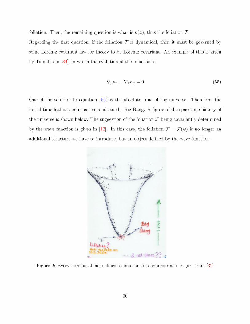
One of the solution to equation (55) is the absolute time of the universe. Therefore, the

initial time leaf is a point corresponds to the Big Bang. A figure of the spacetime history of

the universe is shown below. The suggestion of the foliation F being covariantly determined

by the wave function is given in [12]. In this case, the foliation F = F(ψ) is no longer an

additional structure we have to introduce, but an object defined by the wave function.

Figure 2: Every horizontal cut defines a simultaneous hypersurface. Figure from [32]

36

6.2 Synchronised trajectories

Synchronised trajectories is a method proposed in [29] and [25]. And this method still

involves some foliation like structure. We will mainly follow [29] for the following discussion.

Suppose we have a system of N spinless relativistic particles, the wave function satisfies N

Klein-Gordon equation, and thus

(N∑a

ηµν∂µa∂

νa + nm2)ψ(x1, ..., xn) = 0 (56)

where ηµν has signature (+,−,−,−) and xi = (ti, ~xi). It is well known that there exists a

conserved 4-current of the form ψ∗∂µψ − ψ∂muψ∗ so we define

jµa (x1, ..., xn) = i(ψ∗∂µaψ − ψ∂µaψ∗) (57)

thus ∂aµjµa = 0.

Then we put the wave function into polar form ReiS, where R and S are the function

of xa = (ta, ~xa). Substituting it into the Klein-Gordon equation (56), then the real and

imaginary respectively are

ηµν∂µa∂

νaR−R∂aµS∂µaS + nm2R = 0 (58)

∂aµR∂µaS + ∂µaR∂aµS +Rηµν∂

µa∂

νaS = 0 (59)

where the summation of the index a is accounted for by the repeated index. And they are

usually put in the following form

37

− 1

2m∂aµS∂

µaS +

nm2

2+Q = 0 (60)

where Q = 12mR

ηµν∂µa∂

νaR.

∂µa (R2∂aµS) = 0 (61)

These are the relativistic version of equation (22) and (23). Then a pilot-wave model can be

developed by introducing the equation

dXµa

dλ= − 1

m∂µaS(x1, ..., xN)

∣∣∣xa=Xa(λ)

(62)

where λ is a parametrization factor of the actual spacetime curve Xµa of the a-th particle in

Minkowski spacetime. Similar to the non-relativistic case, the multi-time wave function is

responsible for generating a time dependent vector field in the spacetime configuration space

and (X1(λ), ..., XN(λ)) is the integral curve of the vector field. Even though equation is

non-local, it is Lorentz invariant. Note that all trajectories are parameterized in terms of the

same factor λ. This is the reason this method is called synchronised trajectories. Actually,

one can parameterizes each trajectory with a different parameter once the trajectory has

been found.

A problem of this formulation is that since the Klein-Gordon equation is second-derivative

in time, the quantity |ψ|2 cannot be interpreted as probability density. In standard quantum

mechanics, one circumvents this problem by second quantization in which ψ is no longer the

probability density, but a field. However, the author suggested that the failure of interpreting

|ψ|2 as probability density does not mean probability cannot be calculated. More precisely,

the author firstly argued that if fundamentally ψ is to be regarded as a field, then there is

no clear connection on why the probabilistic interpretation of |ψ|2 has such as a good agree-

ment with experimental results in non-relativistic limit. Since relativistic quantum theory

38

lacks statistical transparency (i.e the probability of particle position can be calculated by

only knowing the wave function), it is natural that |ψ|2 cannot be interpreted as probability

density. Yet if one assumes that particle trajectories exist, then statistical predictions can

still be obtained. Therefore, because Bohmian mechanics assumes the existence of particle

trajectories, it is not necessary to ’promote’ to status of the wave function to field in relativis-

tic Bohmian mechanics. However, there are a few problems such as superluminal velocities

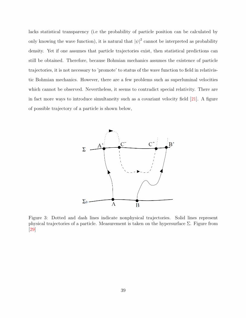
which cannot be observed. Nevertheless, it seems to contradict special relativity. There are

in fact more ways to introduce simultaneity such as a covariant velocity field [21]. A figure

of possible trajectory of a particle is shown below,

Figure 3: Dotted and dash lines indicate nonphysical trajectories. Solid lines representphysical trajectories of a particle. Measurement is taken on the hypersurface Σ. Figure from[29]

39

7 Bohmian Mechanics and QFT

As Bohmian mechanics accounts for every quantum phenomena like the orthodox quantum

mechanics, it is then natural to extend Bohmian mechanics to quantum field theory which

is considered as one of most fundamental theory of reality (See [38] for an overview of field

beable Bohmian type field theory). In this section, two Bohmian type field theories based on

field beable, which are examples in [38], will be presented. Then, followed by a brief dicussion

of Bell-type theory based on particle beable. (See [39] and [40] for an overview) Quantum

field theory is usually mathematically ill-defined without regularization and renormalization.

In this section, it is assumed that the theory presented can be regularized and renormalized.

7.1 Schrodinger Field

Consider the following Lagrangian density of the Schrodinger field

L =[ i

2(ψ∗ψ − ψψ∗) +

1

2mψ∗∇2ψ

](63)

Separate ψ into real and imaginary part, ψ = ψr + iψi. Then, the Lagrangian is

L =

∫d3xL =

∫d3x[(ψrψi + ψiψr) +

1

2m(ψr∇2ψr + ψi∇2ψi + iψr∇2ψi + iψi∇2ψr)

](64)

the last two terms cancel each other by integration by parts and the assumption that field ψ

goes to zero at spatial infinity. The conjugate momentum are the following,

Πψr = ψi

Πψi = −ψr(65)

40

Then, the Hamiltonian is

H =

∫d3xH =

∫d3xψrΠψr + ψiΠψi − L =

−1

2m

∫d3x[ψr∇2ψr + ψi∇2ψi

](66)

By equation (65), since ψr and ψi cannot be expressed in terms of ψr, ψi, Πψr and Πψi , there

are two constraints. Quantization of system with constraints are treated differently. Discus-

sion and analysis of quantization of such type can be found in [38] and [10]. The unconstrained

variables can be separated from the constrained ones by a canonical transformation.

ψr =1√2

(φ+ φ)

Πψr =1√2

(Πφ + Πφ)

ψi =1√2

(Πφ − Πφ)

Πψi =1√2

(φ− φ)

(67)

Then the physical Hamiltonian in which φ = Πφ = 0 is

H =

∫d3xH =

−1

4m

∫d3x[φ∇2φ+ Πφ∇2Πφ

](68)

Then the system is quantized using canonical quantization in which φ and Πφ are promoted

to operators φ and Πφ. Also, by imposing the following commutation relation

[φ(~x), Πφ(~y)] = iδ(~x− ~y) (69)

In Schrodinger picture, the time dependence lies in the state |Ψ〉 instead of the operators.

The Hamiltonian in operator form is

41

H =−1

4m

∫d3x[φ∇2φ+ Πφ∇2Πφ

](70)

In Schrodinger representation, one lets φ |φ〉 = φ(~x) |φ〉, which is analogous to the position

basis in usual quantum mechanics. In this basis, the conjugate momentum operator takes

the form of −i δδφ

. Then the evolution of the wave functional 〈φ|Ψ〉 = Ψ[φ(~x), t] is governed

by the Schrodinger equation, in this case, a functional differential equation.

i∂Ψ[φ(~x), t]

∂t=−1

4m

∫d3x[φ(~x)∇2φ(~x) + (−i δ

δφ(x))∇2(−i δ

δφ(x))]Ψ[φ(~x), t] (71)

It can be rewritten as

i∂Ψ[φ(~x), t]

∂t=−1

2

∫ ∫d3xd3y

[ δ

δφ(~x)h(~x, ~y)

δ

δφ(~x)− φ(~x)h( ~x, ~y)φ(~y)

]Ψ[φ(~x), t] (72)

where h( ~x, ~y) = −12m∇2δ(~x−~y). In order to construct a Bohmian type field theory, one has to

postulate a addition beable and its equation of motion. Therefore, one should first look for

an equation analogous to equation (21) to get guiding equation of field configuration. The

continuity equation associated to equation (72) can be derived in a similar way as described in

section (3) for the continuity equation for the Schrodinger equation (17) in standard quantum

mechanics. Since ~x and ~y are just the continuous versions of the discrete indices in classical

mechanics. Therefore, one can go to discrete case to calculate the discrete version. Then

replacing the sum by an integral and discrete indices by the continuous ones ~x and ~y. One

then can verify that the continuity equation is

∂|Ψ[φ(~x), t]|2

∂t+

∫d3x

δj[φ(~x)]

δφ(~x)= 0 (73)

where j[φ(~x)] = −i2

∫d3yh(~x, ~y)(Ψ∗ δΨ

δφ(~y)− Ψ δΨ∗

δφ(~y)). Let Ψ[φ(~x)] = |Ψ[φ]|eiS[φ] and substitute

it into the expression of j,

42

j[φ(~x)] =

∫d3yh(~x, ~y)|Ψ|2 δS[φ]

δ(y)(74)

By comparing this the expression of Bohmian velocity (18). One then defines the following

φ(~x) =j[φ(~x)]

|Ψ|2=

∫d3yh(~x, ~y)

δS[φ]

δ(y)(75)

Unlike the quantization of the Schrodinger field in standard quantum field theory, one has to

single out the physical degree of freedom of the field in a Bohmian type field theory because

the addition variable (beable) is related to the ontology of the theory which should give an

image of the physical world. Therefore, if a unphysical field beable is treated equally as

physical ones, it is unclear what physical entity this field corresponds to.

7.2 Electromagnetic Field

There are two ways to construct a Bohmian type theory for the electromagnetic field. The

first was done by Bohm in his 1952 paper [7], another was done by Valentini in [41]. In this

section, we follow a similar approach by Bohm.

Consider the following Lagrangian,

L =

∫d3xL =

∫d3x− 1

4FµνF

µν (76)

and the conjugate momentum field is

Πµ =∂L

∂(∂0Aµ)= ∂µA0 − ∂0Aµ = F µ0 (77)

By substituting L into Euler-Lagrange equation, one gets the equation of motion

43

∂µFµν = 0 (78)

this implies two constraints

Π0 = 0

∂iΠi = 0

(79)

These two constraints implies there are two gauge variables and one of them is A0. To

identify, one can first preform a canonical transformation then express the transverse and

longitudinal part in terms of them. Hence, showing that the second constraint implies the

longitudinal part is a gauge variable. However, the same result can be obtained by simply

imposing Coulomb gauge ∂iAi = 0 and A0 = 0 . By introducing the projection operator

Pij =∂i∂j∇2

(80)

then the longitudinal part is

ALi (~x) = PijAj(~x) =∂i∂j∇2

Aj(~x) (81)

by the Coulomb gauge condition ALi (~x) = 0. Hence,the gauge is completely fixed. And the

physical variable is the transverse part

ATi (~x) = (δij − Pij)Aj(~x) (82)

and Ai(~x) = ALi (~x)+ATi (~x). By equation (76) and (77), the Hamiltonian in original canonical

pair Ai and Πi is

44

H =

∫d3xΠµAµ − L

H =

∫d3xF µ0(F0µ + ∂µA0) +

1

4FµνF

µν

H =

∫d3xE2 + Ei∂iA0 +

1

2(B2 − E2)

H =

∫d3x

1

2ΠiΠi +

1

4FijF

ij

(83)

On the second line we used ∂oAµ = F0µ + ∂µA0. From the second last to the last line, the

term Ei∂iA0 disappears because of integration by parts and the use of constraints. Then, E

and B is expressed in terms of the conjugate momentum field Πi and Fij. This can be easily

verified by writing F in its matrix form. Expanding the second term gives

1

4(∂iAj − ∂jAi)2 =

1

2(∂iAj∂iAj − ∂iAj∂jAi)

= −1

2(Ai∂j∂jAi)

(84)

since partial derivatives commute, then by integration by parts, the gauge condition and

the assumption that Ai goes to 0 at spatial infinity, ∂iAj∂jAi becomes 0. Then by Ai(~x) =

ALi (~x) + ATi (~x) and the result of the gauge condition ALi (~x) = 0 the only physical field

variables are ATi (~x), the physical Hamiltonian is

H =

∫d3x

1

2ΠTi ΠT

i −1

2(Ai∇2Ai) (85)

where ΠTi is the conjugate momentum field of ATi . In canonical quantization, the field ATi

and its conjugate momentum ΠTi become operators ATi and ΠT

i which take the following form

in Schrodinger representation

ATi (~x) −→ ATi (~x)

ΠTi −→ −i

δ

δATi (~x)

(86)

45

Therefore, the physical Hamiltonian in Schrodinger representation is

H =1

2

∫d3x(− δ2

δATi (~x)δATi (~x)− (ATi ∇2ATi )

)(87)

Hence, the wave functional will Ψ[ATi (~x), t] evolves according to the following Schrodinger

equation

i∂Ψ

∂t=

1

2

∫d3x(− δ2

δATi (~x)δATi (~x)− (ATi ∇2ATi )

)Ψ[ATi (~x), t] (88)

The continuity equation can be found in a similar as in section (3).

∂|Ψ|2

∂t+

∫d3x

δ

δATiJ [ATi ] (89)

where J = i2[Ψ∗ δΨ

δATi− Ψ δΨ∗

δATi]. Then by Ψ = |Ψ|eiS where S = S[ATi , t], then J = |Ψ|2[ δS

δATi].

Hence, postulating that ATi as beable whose evolution is determined by

ATi (~x) =δS[ATi ]

δATi (~x)(90)

7.3 Problems of field ontology

There are a few problems with using field configuration as beable. The first is that different

macrostates do not seem to be supported by some non-overlapping wave functionals. In usual

Bohmian mechanics, we assume that a pointer pointing a two different directions corresponds

to two actual configurations which are supported by two non-overlapping wave functions ψ1

and ψ2. Mathematically,

|ψ|2 = |ψ1|2 + |ψ2|2 (91)

where ψ is the total wave function. We use this assumption in section (4) in which they

are wave packets. Therefore, in the field ontology case, one should expect that distinct mar-

46

costates or field configurations should be described by some non-overlapping wave functionals.

Consider the one particle state of the Schrodinger field, whose functional form is

Ψ1[φ(~x), t] =√

2

∫d3xψ(~x, t)φ(~x)Ψ0[φ(~x), t] (92)

where Ψ0[φ(~x), t] is the wave functional of the vacuum state, ψ(~x, t) is normalized solu-

tion of the Schrodinger equation. Ψ0[φ(~x), t] can be obtained by first realising that ψ =

b∫d3ke−i

~k·~xa(~k), where a(~k) is the annihilation operator and b just a constant, is the field

operator of the usual quantized version of Schrodinger field and can be written as 1√2(φ+ δ

δφ)

in Schrodinger representation. Then by the condition a(~k) |Ψ0〉 = 0, one can get the func-

tional form of the vacuum state. After that, the one particle state is obtained by the action

of the conjugate field operator ψ∗ on the vacuum state. Then consider the absolute value

squared of Ψ1[φ(~x), t],

|Ψ1[φ(~x), t]|2 = 2

∣∣∣∣∫ d3xψ(~x)φ(~x)

∣∣∣∣2|Ψ0[φ(~x), t]|2 (93)

whose maximum can be found by requiring the functional derivative equal to zero. Let

α[φ(~x)] =∫d3xψ(~x)φ(~x),

δ|Ψ1[φ(~x), t]|2

δφ= 2

δ

δφ

[|α|2|Ψ0[φ(~x), t]|2

]= 2[δ|α|2δφ|Ψ0|2 + |α|2 δ|Ψ0|2

δφ

] (94)

then use the product rule for δ|α|2δφ

and δ|Ψ0|2δφ

and the following

α

δφ= ψ

α∗

δφ= ψ∗

(95)

47

Ψ0

δφ= −φΨ0

Ψ∗0δφ

= −φΨ0

(96)

then maximum condition, one finds that the maximum is at

φ(~x) =1

2

(ψ∗α∗

+ψ

α

)(97)

Consider a linear combination of one particle states Ψ[φ(~x), t] = N(Ψ(1)1 [φ(~x), t]+Ψ

(2)1 [φ(~x), t]).

If Ψ(1)1 [φ(~x), t] and Ψ

(2)1 [φ(~x), t] are non-overlapping wave functionals, then we would expect

the analogue of equation (91),

|Ψ[φ(~x), t]|2 = N2(∣∣∣Ψ(1)

1 [φ(~x), t]∣∣∣2 +

∣∣∣Ψ(2)1 [φ(~x), t]

∣∣∣2) (98)

which has to two maxima one at 12

(ψ∗(1)

α∗(1)

+ψ(1)

α(1)

)and another at 1

2

(ψ∗(2)

α∗(2)

+ψ(2)

α(2)

). However,

the maximum of |Ψ[φ(~x), t]|2 is 12

((ψ(1)+ψ(2))

∗

(α(1)+α(2))∗ +

(ψ(1)+ψ(2))

(α(1)+α(2))

)Therefore, this indicates that

Ψ(1)1 [φ(~x), t] and Ψ

(2)1 [φ(~x), t] are overlapping. A detailed discussion and more examples are

given in [38].

Another problem is related to regularization and renormalization. Even though equation

(73) and (89) ensure the conservation of the quantity |Ψ|2, the probability of the actual field

configuration be φ(~x) is |Ψ[φ(~x), t]|2ΠDφ, which the analogue of the quantum equilibrium

hypothesis in the usual Bohmian mechanics, is mathematically ill-defined as one is dealing

with system with an infinity number of degree of freedom. Therefore, regularization and

renormalization are needed. (See [38] for a detailed discussion) In addition, by Bell’s theo-

rem non-locality is unavoidable, thus incompatibility of Lorentz invariant remains as one of

problems just like usual Bohmian mechanics. More examples can be found in [36] and [37].

48

7.4 Bell-type quantum field theories

Bell-type quantum field theories refer to the extension of Bohmian mechanics that incor-

porates creation and annihilation of particles. Unlike the two previous Bohmian type field

theory, the beable is not field, but particle’s worldline, an example is shown in figure (4) at

the end of this section. This extension of Bohmian mechanics was first proposed by Bell [2]

on a lattice and later extended and explored in [13], [9] and many other in the continuum

limit. In this section, we will follow mainly [14].

In usual Bohmian mechanics presented in section (3), the number of particle in the system of

interest (N) is fixed and thus the corresponding configuration space is of finite dimension, 3N.

In order to incorporate particle creation and annihilation, a countably infinite dimensional

configuration space is introduced

Q =∞⋃i=0

Q[i] (99)

where⋃

is the disjoint union,Q[i] is the configuration space representing i number of particles.

For example, Q[1] = R3. The evolution of the system is then represented by some curves in

the configuration space Q. If there is no creation or annihilation event, then the curve will

be continuous and lives in Q[i] and evolves according to the guiding equation. If there is a

creation event, then the trajectory will have a discontinuous jump from the sub-configuration

space Q[i] to Q[i+1] and if it is an annihilation event, then it jumps from Q[i] to Q[i−1]. Just

like usual Bohmian mechanics, the state of system is given by the wave function and its

configuration (ψ,Q). The wave function evolves according to the Schrodinger equation with

the Hamiltonian H = Hfree +Hint. The dynamics of the configuration Q is determined by a

more general guiding equation

dQ(t)

dt= Re

[ψ∗(Q(t))( ˙qψ)(Q(t))

ψ∗(Q(t))ψ(Q(t))

](100)

49

where ˙q = i~ [Hfree, q].

Unlike the usual Bohmian mechanics, there is an additional equation, which determines the

probability of jump per time,

σ(dq|q′) =2

~[Imψ∗(q) 〈q|Hint

∣∣q′⟩ψ(q′)]+

ψ∗(q′)ψ(q′)(101)

where x+ = max(x, 0) is the positive part of x ∈ R. These equations together defines a

stochastic process called the Markov process (see [14] for further analysis). Therefore, this

extension of Bohmian mechanics is no longer deterministic as the ususl Bohmian mechanics

since the jump is described probabilistically. It is shown in [14] that one can associate a

Bell-type QFT for most of the Hamiltonian. For example, for

H = −~2 ∂2

∂x2+ V (x) (102)

then the associated theory is the usual Bohmian mechanics. More examples of the Bell-type

QFT is given in [15].

50

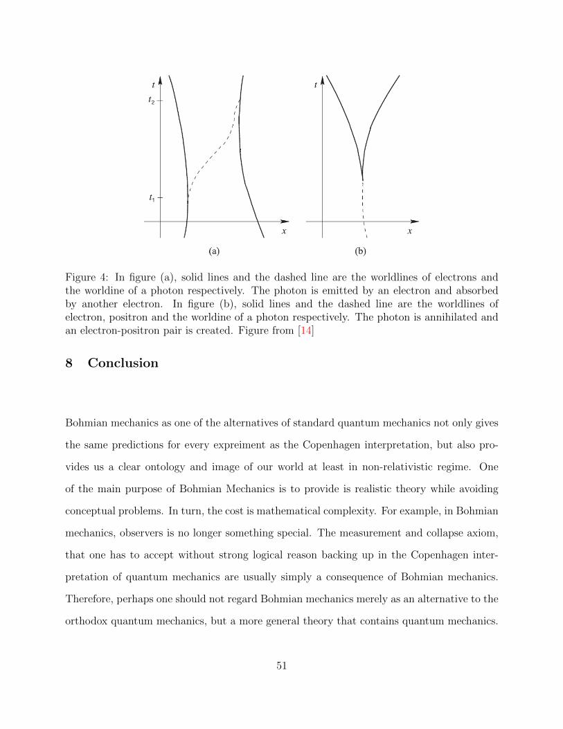
Figure 4: In figure (a), solid lines and the dashed line are the worldlines of electrons andthe worldine of a photon respectively. The photon is emitted by an electron and absorbedby another electron. In figure (b), solid lines and the dashed line are the worldlines ofelectron, positron and the worldine of a photon respectively. The photon is annihilated andan electron-positron pair is created. Figure from [14]

8 Conclusion

Bohmian mechanics as one of the alternatives of standard quantum mechanics not only gives

the same predictions for every expreiment as the Copenhagen interpretation, but also pro-

vides us a clear ontology and image of our world at least in non-relativistic regime. One

of the main purpose of Bohmian Mechanics is to provide is realistic theory while avoiding

conceptual problems. In turn, the cost is mathematical complexity. For example, in Bohmian

mechanics, observers is no longer something special. The measurement and collapse axiom,

that one has to accept without strong logical reason backing up in the Copenhagen inter-

pretation of quantum mechanics are usually simply a consequence of Bohmian mechanics.

Therefore, perhaps one should not regard Bohmian mechanics merely as an alternative to the

orthodox quantum mechanics, but a more general theory that contains quantum mechanics.

51

Despite of its conceptional advantage, namely particles guided by wave, Bohmian mechanics

remains widely unaccepted by the majority of the scientific community (see [34]). From the

analysis of Bohmian mechanics and its extensions in this dissertation, I believe that the two

main reasons of this mass unacceptance of the theory are

• The explicit non-locality in the guiding equation which seems to contradict the spirit of

special relativity. Even though proposals have made, they usually involve some addition

structures like a foliation in order to define simultaneity. Therefore, one might argue

that the theory is not fundamentally Lorentz invariant.

• The lack of consistent choice of beable and mathematics rigour in its extension. Bosonic

particles are better described by field ontology while Fermionic particles seems to be

better described by particle ontology.

To overcome these problems more theoretical development of the theory are needed. Perhaps

the pilot wave picture should be taught in a standard quantum mechanics class in universities

in order to stimulate student to do more research related to the foundation of quantum

mechanics.

52

References

[1] V. Allori, D. Durr, S. Goldstein, and N. Zanghi. Seven steps towards the classical world.

Journal of Optics B: Quantum and Semiclassical Optics, 4(4):S482–S488, Aug 2002.

[2] J. Bell. Quantum field theory of without observers. Physics Reports, 137(1):49 – 54,

1986.

[3] J. S. Bell. On the einstein podolsky rosen paradox. Physics Physique Fizika, 1:195–200,

Nov 1964.

[4] J. S. BELL. On the problem of hidden variables in quantum mechanics. Rev. Mod.

Phys., 38:447–452, Jul 1966.

[5] J. S. Bell and A. Aspect. Speakable and Unspeakable in Quantum Mechanics: Collected

Papers on Quantum Philosophy. Cambridge University Press, 2 edition, 2004.

[6] D. Bohm. A suggested interpretation of the quantum theory in terms of ”hidden”

variables. i. Phys. Rev., 85:166–179, Jan 1952.

[7] D. Bohm. A suggested interpretation of the quantum theory in terms of ”hidden”

variables. ii. Phys. Rev., 85:180–193, Jan 1952.

[8] D. Bohm. Comments on an Article of Takabayasi conserning the Formulation of Quan-

tum Mechanics with Classical Pictures. Progress of Theoretical Physics, 9(3):273–287,

03 1953.

[9] S. Colin. Beables for quantum electrodynamics, 2003.

[10] P. Dirac. Lectures on Quantum Mechanics. Belfer Graduate School of Science, mono-

graph series. Dover Publications, 2001.

53

[11] D. Durr, S. Goldstein, and Z. Nino. Quantum equilibrium and the origin of absolute

uncertainty. Journal of Statistical Physics, 67(5-6):843–907, Jun 1992.

[12] D. Durr, S. Goldstein, T. Norsen, W. Struyve, and N. Zanghı. Can bohmian mechanics

be made relativistic? Proceedings of the Royal Society A: Mathematical, Physical and

Engineering Sciences, 470(2162):20130699, Feb 2014.

[13] D. Durr, S. Goldstein, R. Tumulka, and N. Zanghı. Trajectories and particle creation and

annihilation in quantum field theory. Journal of Physics A: Mathematical and General,

36(14):4143–4149, Mar 2003.

[14] D. Durr, S. Goldstein, R. Tumulka, and N. Zanghı. Bohmian mechanics and quantum

field theory. Physical Review Letters, 93(9), Aug 2004.

[15] D. Durr, S. Goldstein, R. Tumulka, and N. Zanghı. Quantum hamiltonians and stochas-

tic jumps. Communications in Mathematical Physics, 254(1):129–166, Nov 2004.

[16] D. Durr, S. Goldstein, and N. Zanghı. Bohmian mechanics and the meaning of the wave

function, 1995.

[17] D. Durr and S. Teufel. Bohmian Mechanics: The Physics and Mathematics of Quantum

Theory. Springer Berlin Heidelberg, 2009.

[18] M. Esfeld, D. Lazarovici, M. Hubert, and D. Durr. The ontology of bohmian mechanics,

2014.

[19] H. Everett. The many-worlds interpretation of quantum mechanics. Thesis, 1957.

[20] G. C. Ghirardi, A. Rimini, and T. Weber. Unified dynamics for microscopic and macro-

scopic systems. Phys. Rev. D, 34:470–491, Jul 1986.

[21] S. Goldstein and S. Teufel. Quantum spacetime without observers: ontological clarity

and the conceptual foundations of quantum gravity, 1999.

54

[22] S. Goldstein and R. Tumulka. Opposite arrows of time can reconcile relativity and

nonlocality. Classical and Quantum Gravity, 20(3):557–564, Jan 2003.

[23] S. Goldstein and N. Zanghı. Reality and the role of the wavefunction in quantum theory,

2011.

[24] P. R. Holland. The Quantum Theory of Motion: An Account of the de Broglie-Bohm

Causal Interpretation of Quantum Mechanics. Cambridge University Press, 1993.

[25] G. Horton and C. Dewdney. A non-local, lorentz-invariant, hidden-variable interpreta-

tion of relativistic quantum mechanics based on particle trajectories. Journal of Physics

A: Mathematical and General, 34(46):9871–9878, Nov 2001.

[26] S. Kocsis, B. Braverman, S. Ravets, M. Stevens, R. Mirin, L. Shalm, and A. Steinberg.

Observing the average trajectories of single photons in a two-slit interferometer. Science

(New York, N.Y.), 332:1170–3, 06 2011.

[27] M. Lienert, S. Petrat, and R. Tumulka. Multi-time wave functions. Journal of Physics:

Conference Series, 880:012006, Aug 2017.

[28] L. Maccone. A simple proof of bell’s inequality. American Journal of Physics,

81(11):854–859, Nov 2013.

[29] H. Nikolic. Relativistic quantum mechanics and the bohmian interpretation. Foundations

of Physics Letters, 18(6):549–561, Nov 2005.

[30] T. Norsen. The pilot-wave perspective on spin. American Journal of Physics,

82(4):337–348, Apr 2014.

[31] X. Oriols and J. Mompart. Overview of bohmian mechanics. Applied Bohmian Mechan-

ics: From Nanoscale Systems to Cosmology, 06 2012.

55

[32] R. Penrose. On the gravitization of quantum mechanics 2: Conformal cyclic cosmology.

Foundations of Physics, 44:873–890, 08 2013.

[33] C. Philippidis, C. Dewdney, and B. Hiley. Quantum interference and the quantum

potential. Il Nuovo Cimento B, 52:15–28, 07 1979.

[34] M. Schlosshauer, J. Kofler, and A. Zeilinger. A snapshot of foundational attitudes toward

quantum mechanics. Studies in History and Philosophy of Science Part B: Studies in

History and Philosophy of Modern Physics, 44(3):222–230, Aug 2013.

[35] E. J. Squires. A local hidden-variable theory that, fapp, agrees with quantum theory.

Physics Letters A, 178(1):22 – 26, 1993.

[36] W. Struyve. The de broglie-bohm pilot-wave interpretation of quantum theory, 2005.

[37] W. Struyve. A new pilot-wave model for quantum field theory. AIP Conference Pro-

ceedings, 2006.

[38] W. Struyve. Pilot-wave approaches to quantum field theory. Journal of Physics: Con-

ference Series, 306:012047, Jul 2011.

[39] R. Tumulka. The “unromantic pictures” of quantum theory. Journal of Physics A:

Mathematical and Theoretical, 40(12):3245–3273, Mar 2007.

[40] R. Tumulka. On bohmian mechanics, particle creation, and relativistic space-time:

Happy 100th birthday, david bohm! Entropy, 20(6):462, Jun 2018.

[41] A. Valentini. On the pilot-wave theory of classical, quantum and subquantum physics.

PhD thesis, SISSA, Trieste, 1992.

56