
Overview - NYU Computer Sciencefergus/teaching/comp_photo/9-vide… · · 2008-04-07• Special...
19
4/7/2008 1 Video Lecture 9 Overview • Optical flow • Motion Magnification • Colorization Overview • Optical flow • Motion Magnification • Colorization Optical flow Combination of slides from Rick Szeliski, Steve Seitz, Alyosha Efros and Bill Freeman Motion estimation: Optical flow Will start by estimating motion of each pixel separately Then will consider motion of entire image Why estimate motion? Lots of uses • Track object behavior • Correct for camera jitter (stabilization) • Align images (mosaics) • 3D shape reconstruction • Special effects
Transcript of Overview - NYU Computer Sciencefergus/teaching/comp_photo/9-vide… · · 2008-04-07• Special...

4/7/2008
1
Video
Lecture 9
Overview
• Optical flow
• Motion Magnification
• Colorization
Overview
• Optical flow
• Motion Magnification
• Colorization
Optical flowCombination of slides from Rick Szeliski, Steve Seitz,
Alyosha Efros and Bill Freeman
Motion estimation: Optical flow
Will start by estimating motion of each pixel separatelyThen will consider motion of entire image
Why estimate motion?Lots of uses
• Track object behavior• Correct for camera jitter (stabilization)• Align images (mosaics)• 3D shape reconstruction• Special effects

4/7/2008
2
Problem definition: optical flow
How to estimate pixel motion from image H to image I?• Solve pixel correspondence problem
– given a pixel in H, look for nearby pixels of the same color in I
Key assumptions• color constancy: a point in H looks the same in I
– For grayscale images, this is brightness constancy• small motion: points do not move very far
This is called the optical flow problem
Optical flow constraints (grayscale images)
Let’s look at these constraints more closely• brightness constancy: Q: what’s the equation?
• small motion: (u and v are less than 1 pixel)– suppose we take the Taylor series expansion of I:
H(x,y)=I(x+u, y+v)
Optical flow equationCombining these two equations
In the limit as u and v go to zero, this becomes exact
Optical flow equation
Q: how many unknowns and equations per pixel?
Intuitively, what does this constraint mean?
• The component of the flow in the gradient direction is determined
2 unknowns, one equation
p g• The component of the flow parallel to an edge is unknown
This explains the Barber Pole illusionhttp://www.sandlotscience.com/Ambiguous/Barberpole_Illusion.htmhttp://www.liv.ac.uk/~marcob/Trieste/barberpole.html
http://en.wikipedia.org/wiki/Barber's_pol
Aperture problem Aperture problem

4/7/2008
3
Solving the aperture problemHow to get more equations for a pixel?
• Basic idea: impose additional constraints– most common is to assume that the flow field is smooth locally– one method: pretend the pixel’s neighbors have the same (u,v)
» If we use a 5x5 window, that gives us 25 equations per pixel!
RGB versionHow to get more equations for a pixel?
• Basic idea: impose additional constraints– most common is to assume that the flow field is smooth locally– one method: pretend the pixel’s neighbors have the same (u,v)
» If we use a 5x5 window, that gives us 25*3 equations per pixel!
Note that RGB is not enough to disambiguate because R, G & B are correlatedJust provides better gradient
Lukas-Kanade flowProb: we have more equations than unknowns
Solution: solve least squares problem• minimum least squares solution given by solution (in d) of:
• The summations are over all pixels in the K x K window• This technique was first proposed by Lukas & Kanade (1981)
Aperture Problem and Normal Flow
0
0
=•∇
=++
UI
IvIuI tyxr
The gradient constraint:
Defines a line in the (u v) spaceDefines a line in the (u,v) space
u
v
II
IIu t
∇∇
∇−=⊥
Normal Flow:
Combining Local Constraints
v11tIUI −=•∇
22tIUI −=•∇
u
t
33tIUI −=•∇
etc.
Conditions for solvability• Optimal (u, v) satisfies Lucas-Kanade equation
When is This Solvable?• ATA should be invertible • ATA should not be too small due to noise
– eigenvalues λ1 and λ2 of ATA should not be too small• ATA should be well-conditioned
– λ1/ λ2 should not be too large (λ1 = larger eigenvalue)ATA is solvable when there is no aperture problem

4/7/2008
4
Local Patch Analysis Edge
– large gradients, all the same– large λ1, small λ2
Low texture region
– gradients have small magnitude– small λ1, small λ2
High textured region
– gradients are different, large magnitudes– large λ1, large λ2
ObservationThis is a two image problem BUT
• Can measure sensitivity by just looking at one of the images!• This tells us which pixels are easy to track, which are hard
– very useful later on when we do feature tracking...
Errors in Lukas-KanadeWhat are the potential causes of errors in this procedure?
• Suppose ATA is easily invertible• Suppose there is not much noise in the image
When our assumptions are violated• Brightness constancy is not satisfied• The motion is not small• A point does not move like its neighbors• A point does not move like its neighbors
– window size is too large– what is the ideal window size?

4/7/2008
5
Iterative RefinementIterative Lukas-Kanade Algorithm
1. Estimate velocity at each pixel by solving Lucas-Kanade equations2. Warp H towards I using the estimated flow field
- use image warping techniques3. Repeat until convergence
Optical Flow: Iterative Estimation
Initial guess: Estimate:
estimate update
xx0
Estimate:
(using d for displacement here instead of u)
Optical Flow: Iterative Estimation
estimate update
Initial guess: Estimate:
xx0
Estimate:
Optical Flow: Iterative Estimation
Initial guess: Estimate:Initial guess: Estimate:
estimate update
xx0
Estimate:Estimate:
Optical Flow: Iterative Estimation
xx0
Optical Flow: Iterative EstimationSome Implementation Issues:
• Warping is not easy (ensure that errors in warping are smaller than the estimate refinement)
• Warp one image, take derivatives of the other so you don’t need to re-compute the gradient after each iteration.
• Often useful to low-pass filter the images before motion estimation (for better derivative estimation, and linear
i ti t i i t it )approximations to image intensity)
4/7/2008
6
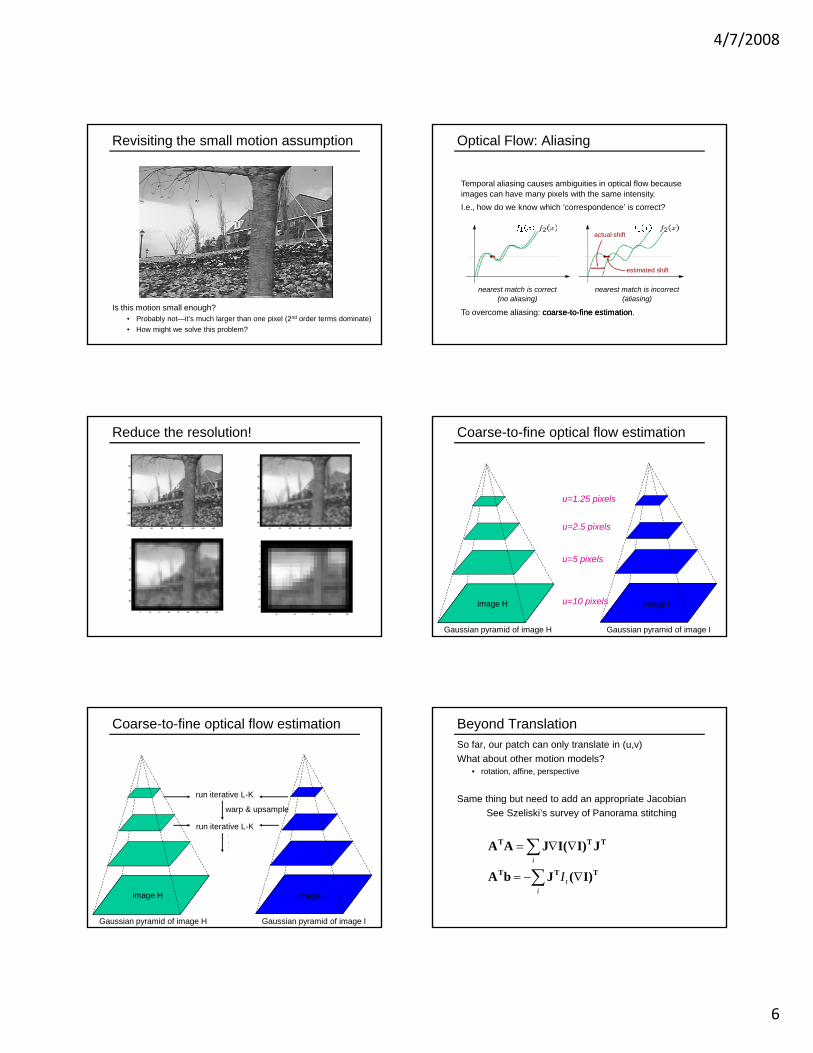
Revisiting the small motion assumption
Is this motion small enough?• Probably not—it’s much larger than one pixel (2nd order terms dominate)• How might we solve this problem?
Optical Flow: Aliasing
Temporal aliasing causes ambiguities in optical flow because images can have many pixels with the same intensity.I.e., how do we know which ‘correspondence’ is correct?
actual shift
nearest match is correct (no aliasing)
nearest match is incorrect (aliasing)
To overcome aliasing: coarsecoarse--toto--fine estimationfine estimation.
actual shift
estimated shift
Reduce the resolution!
u=2 5 pixels
u=1.25 pixels
Coarse-to-fine optical flow estimation
image Iimage H
Gaussian pyramid of image H Gaussian pyramid of image I
image Iimage H u=10 pixels
u=5 pixels
u=2.5 pixels
Coarse-to-fine optical flow estimation
run iterative L-K
warp & upsample
image Iimage J
Gaussian pyramid of image H Gaussian pyramid of image I
image Iimage H
run iterative L-K...
Beyond TranslationSo far, our patch can only translate in (u,v)What about other motion models?
• rotation, affine, perspective
Same thing but need to add an appropriate Jacobian See Szeliski’s survey of Panorama stitchingy g
∑
∑∇−=
∇∇=
it
i
I TTT
TTT
I)(JbA
JI)I(JAA

4/7/2008
7
Feature-based methods (e.g. SIFT+Ransac+regression)• Extract visual features (corners, textured areas) and track them over
multiple frames• Sparse motion fields, but possibly robust tracking• Suitable especially when image motion is large (10-s of pixels)
Recap: Classes of Techniques
Direct-methods (e.g. optical flow)• Directly recover image motion from spatio-temporal image brightness
variations• Global motion parameters directly recovered without an intermediate
feature motion calculation• Dense motion fields, but more sensitive to appearance variations• Suitable for video and when image motion is small (< 10 pixels)
Overview
• Optical flow
• Motion Magnification
• Colorization
Motion MagnificationMotion Magnification
Ce Liu Antonio Torralba William T. Freeman
Frédo Durand Edward H. Adelson
Computer Science and Artificial Intelligence Laboratory
Massachusetts Institute of Technology
Motion MicroscopyMotion Microscopy
How can we see all the subtle motions in a video sequence?
Original sequence Magnified sequence
Naïve ApproachNaïve Approach
• Magnify the estimated optical flow field• Rendering by warping
Original sequence Magnified by naïve approach
Layer-based Motion Magnification Processing PipelineLayer-based Motion Magnification Processing Pipeline
Input raw video sequence
Video Registration
Feature pointtracking
Trajectory clustering
Dense optical flow interpolation
Layer segmentation
Magnification,texture fill-in,
rendering
Output magnified video sequence
Layer-based motion analysis
Stationary camera, stationary background
User interaction

4/7/2008
8
Layer-based Motion Magnification Video RegistrationLayer-based Motion Magnification Video Registration
Input raw video sequence
Video Registration
Feature pointtracking
Trajectory clustering
Dense optical flow interpolation
Layer segmentation
Magnification,texture fill-in,
rendering
Output magnified video sequence
Layer-based motion analysisUser interaction
Stationary camera, stationary background
Robust Video RegistrationRobust Video Registration
• Find feature points with Harris corner detector on the reference frame
• Brute force tracking feature points
• Select a set of robust feature points with inlier and outlier estimation (most from the rigid background)
• Warp each frame to the reference frame with a global affine transform
Motion Magnification Pipeline Feature Point TrackingMotion Magnification Pipeline Feature Point Tracking
Input raw video sequence
Video Registration
Trajectory clustering
Feature pointtracking
Dense optical flow interpolation
Layer segmentation
Magnification,texture fill-in,
rendering
Output magnified video sequence
Layer-based motion analysisUser interaction
Challenges (1)Challenges (1)
Adaptive Region of SupportAdaptive Region of Support
• Brute force search Confused by occlusion !
• Learn adaptive region of support using expectation-maximization (EM) algorithmregion of support
time
time
Challenges (2)Challenges (2)

4/7/2008
9
Trajectory PruningTrajectory Pruning
• Tracking with adaptive region of support Nonsense at full occlusion!
• Outlier detection and removal by interpolation
time
inlier probability
Outliers
Comparison Comparison
Without adaptive region of support and trajectory pruningWith adaptive region of support and trajectory pruning
Motion Magnification Pipeline Trajectory ClusteringMotion Magnification Pipeline Trajectory Clustering
Input raw video sequence
Video Registration
Feature pointtracking
Trajectory clustering
Dense optical flow interpolation
Layer segmentation
Magnification,texture fill-in,
rendering
Output magnified video sequence
Layer-based motion analysisUser interaction
Normalized Complex CorrelationNormalized Complex Correlation• The similarity metric should
be independent of phase and magnitude
• Normalized complex correlation
∑∑∑=
tt
t
tCtCtCtC
tCtCCCS
)()()()(
|)()(|),(
2211
221
21
Spectral ClusteringSpectral Clustering
Two clustersTrajectory
ry
Affinity matrix Clustering Reordering of affinity matrix
Traj
ecto
Clustering ResultsClustering Results

4/7/2008
10
Motion Magnification Pipeline Dense Optical Flow FieldMotion Magnification Pipeline Dense Optical Flow Field
Input raw video sequence
Video Registration
Feature pointtracking
Trajectory clustering
Dense optical flow interpolation
Layer segmentation
Magnification,texture fill-in,
rendering
Output magnified video sequence
Layer-based motion analysisUser interaction
From Sparse Feature Points to Dense Optical Flow FieldFrom Sparse Feature Points to Dense Optical Flow Field• Interpolate dense
optical flow field using locally weighted linear
Flow vectors of clustered sparse feature points
Dense optical flow field of cluster 1 (leaves)
Dense optical flow field of cluster 2 (swing)
Cluster 1: leavesCluster 2: swing
gregression
Motion Magnification Pipeline Layer SegmentationMotion Magnification Pipeline Layer Segmentation
Input raw video sequence
Video Registration
Feature pointtracking
Trajectory clustering
Dense optical flow interpolation
Magnification,texture fill-in,
rendering
Output magnified video sequence
Layer-based motion analysisUser interaction
Layer segmentation
Motion Layer AssignmentMotion Layer Assignment
• Assign each pixel to a motion cluster layer, using four cues:– Motion likelihood—consistency of pixel’s intensity if it moves with
the motion of a given layer (dense optical flow field)
– Color likelihood—consistency of the color in a layer
– Spatial connectivity—adjacent pixels favored to belong the same group
– Temporal coherence—label assignment stays constant over time
• Energy minimization using graph cuts
Segmentation ResultsSegmentation Results
• Two additional layers: static background and outlieroutlier
Motion Magnification Pipeline Editing and RenderingMotion Magnification Pipeline Editing and Rendering
Input raw video sequence
Video Registration
Feature pointtracking
Trajectory clustering
Dense optical flow interpolation
Layer segmentation
Magnification,texture fill-in,
rendering
Output magnified video sequence
Layer-based motion analysisUser interaction

4/7/2008
11
Layered Motion Representation for Motion ProcessingLayered Motion Representation for Motion Processing
Background Layer 1 Layer 2
Layer mask
Occluding layers
Appearance for each layer before texture filling-in
Appearance for each layer after texture filling-in
Appearance for each layer after user editing
VideoVideo
Motion MagnificationMotion Magnification
Is the Baby Breathing?Is the Baby Breathing? Are the Motions Real?Are the Motions Real?
Original Magnified
t tx x
yy
Are the Motions Real?Are the Motions Real?
Original Magnified
time time
Original
Magnified
ApplicationsApplications
• Education
• Entertainment
• Mechanical engineeringMechanical engineering
• Medical diagnosis

4/7/2008
12
ConclusionConclusion
• Motion magnification– A motion microscopy technique
• Layer-based motion processing systemLayer based motion processing system– Robust feature point tracking
– Reliable trajectory clustering
– Dense optical flow field interpolation
– Layer segmentation combining multiple cues
Thank you!Thank you!
Motion Magnification
Ce Liu Antonio Torralba William T. Freeman Frédo Durand Edward H. Adelson
Computer Science and Artificial Intelligence Laboratory
Massachusetts Institute of Technology
Overview
• Optical flow
• Motion Magnification
• Colorization
Colorization Using Optimization
Anat Levin Dani Lischinski Yair Weiss
School of Computer Science and Engineering
The Hebrew University of Jerusalem, Israel
Colorization
Colorization: a computer-assisted process of adding color to a monochrome image or movie. (Invented by Wilson Markle, 1970)
Motivation
• Colorizing black and white movies and TV shows
Earl Glick (Chairman, Hal Roach Studios), 1984:“You couldn't make Wyatt Earp today for $1 million an episode. But for $50,000 a segment, you can turn it into color and have a brand new series with no residuals to pay”

4/7/2008
13
Motivation
• Colorizing black and white movies and TV shows
• Recoloring color images for special effects
Motivation
Typical Colorization Process
Images from: “Yet Another Colorization Tutorial”
http://www.worth1000.com/tutorial.asp?sid=161018
• Delineate region boundary
Typical Colorization Process
Images from: “Yet Another Colorization Tutorial”
http://www.worth1000.com/tutorial.asp?sid=161018
Typical Colorization Process
• Delineate region boundary
• Choose region color from palette.
Images from: “Yet Another Colorization Tutorial”
http://www.worth1000.com/tutorial.asp?sid=161018
• Delineate region boundary
• Choose region color from palette.
Typical Colorization Process
Images from: “Yet Another Colorization Tutorial”
http://www.worth1000.com/tutorial.asp?sid=161018

4/7/2008
14
• Delineate region boundary
• Choose region color from palette.
Typical Colorization Process
Images from: “Yet Another Colorization Tutorial”
http://www.worth1000.com/tutorial.asp?sid=161018
• Delineate region boundary
• Choose region color from palette.
• Track regions across video frames
Video Colorization Process
Colorization Process Discussion
Time consuming and labor intensive
• Fine boundaries. • Failures in tracking.
Colorization by Analogy
A : A’
Hertzmann et al. 2001, Welsh et al. 2002
B : B’
?
Colorization by Analogy
A : A’
Hertzmann et al. 2001, Welsh et al. 2002
B : B’
Colorization by Analogy - Discussion
• Indirect artistic control
• No spatial continuity constraint

4/7/2008
15
Our approach Our approach
Artist scribbles desired colors inside regions
Our approach
Colors are propagated to all pixels
“Nearby pixels with similar intensities should have the same color”
VUY ,⇒Intensity channel Color channels
Propagation using Optimization
“Neighboring pixels with similar intensities should have similar colors”
VUY ,⇒Intensity channel Color channels
Propagation using Optimization
2
)()()()( ∑ ∑ ⎟⎟⎠
⎞⎜⎜⎝
⎛−=
∈r rNsrs sUwrUUJ
• Minimize difference between color at a pixel and an affinityaffinity--weighted averageweighted average of the neighbors
Affinity Functions
22 /))()(( rsYrYrs ew σ−−∝
rσ proportional to local variance

4/7/2008
16
Affinity Functions in Space-Time
22 2/))()(( rsYrYrs ew σ−−∝
i1−i
1+i
2
)()()()( ∑ ∑ ⎟⎟⎠
⎞⎜⎜⎝
⎛−=
∈r rNsrs sUwrUUJ
Minimizing cost function
Minimize:
Since cost is quadratic, minimum can be found by solving sparse system of linear equations.
Subject to labeling constraints
Color Interpolation Coloring Stills
Coloring Stills
Original Colorized

4/7/2008
17
Coloring Stills Coloring Stills
Colorization Challenges Segmentation?
Segmentation aidedNCuts Segmentation
Our result
Segmentation aided colorization
NCuts Segmentation (Shi & Malik 97)
Recoloring
Affinity between pixels – based on intensity AND color similarities.
Recoloring

4/7/2008
18
Recoloring
c.f. “Poisson image editing” Perez et al. SIGGRAPH 2003
Colorizing Video
13 out of 92 frames
Colorizing Video
16 out of 101 frames
Matting as Colorization
Red channel<->matte
Matting as Colorization Future Work:
• Import image segmentation advantages: affinity functions, optimization techniques.
• Alternative color spaces, propagating hue and saturation differently

4/7/2008
19
Summary
• Interface: User scribbles color on a small number of pixels
• Colors propagate in space-time volume respecting intensity boundaries
• Convincing colorization with a small amount of user effort
Code & examples available:
www.cs.huji.ac.i/~yweiss/Colorization/


![Lecture 10 - NYU Computer Sciencefergus/teaching/vision/18_19_parts...Figure from [Fischler & Elschlager 73] History of Parts and Structure approaches • Fischler & Elschlager 1973](https://static.fdocuments.in/doc/165x107/604d2ada84275c165a10e519/lecture-10-nyu-computer-science-fergusteachingvision1819parts-figure-from.jpg)