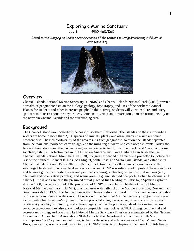
1

Exploring a Marine Sanctuary Lab 2 GEO 465/565

Based on the Mapping an Ocean Sanctuary series of the Center for Image Processing in Education (www.evisual.org)

Overview Channel Islands National Marine Sanctuary (CINMS) and Channel Islands National Park (CINP) provide a wealth of geographic data on the biology, geology, topography, and uses of the northern Channel Islands for students and other interested people. In this activity, students will view, explore, and query spatial data to learn about the physical environment, distribution of bioregions, and the natural history of the northern Channel Islands and the surrounding area.

Background The Channel Islands are located off the coast of southern California. The islands and their surrounding waters are home to more than 2,000 species of animals, plants, and algae, many of which are found nowhere else. The rich biodiversity of the area results from geographic isolation–the islands separated from the mainland thousands of years ago–and the mingling of warm and cold ocean currents. Today the five northern islands and their surrounding waters are protected by “national park” and “national marine sanctuary” status. Protection began in 1938 when Anacapa and Santa Barbara Islands became the Channel Islands National Monument. In 1980, Congress expanded the area being protected to include the rest of the northern Channel Islands (San Miguel, Santa Rosa, and Santa Cruz Islands) and established Channel Islands National Park (CINP). CINP’s jurisdiction includes the islands themselves and the submerged lands within one nautical mile of each island. CINP was established to protect the unique flora and fauna (e.g., pelican nesting areas and pinniped colonies), archeological and cultural remains (e.g., Chumash and other native peoples), and scenic areas (e.g., undisturbed tide pools, Eolian landforms, and caliche). The islands are also the presumed burial place of Juan Rodriquez Cabrillo, a Spanish explorer. Also in 1980, Congress extended the protection of CINP’s waters by establishing Channel Islands National Marine Sanctuary (CINMS), in accordance with Title III of the Marine Protection, Research, and Sanctuaries Act of 1972. The Act recognizes the intrinsic natural, cultural, historical, and economic value of our oceans and coastal waterways. The mission of the National Marine Sanctuary Program is to serve as the trustee for the nation’s system of marine protected areas, to conserve, protect, and enhance their biodiversity, ecological integrity, and cultural legacy. While the primary goals of the sanctuaries are resource protection, they also allow multiple compatible uses such as SCUBA diving, commercial and recreational fishing, and boating. The National Marine Sanctuary Division is administered by the National Oceanic and Atmospheric Association (NOAA), under the Department of Commerce. CINMS encompasses 1,252 square nautical miles, including the near and offshore waters of San Miguel, Santa Rosa, Santa Cruz, Anacapa and Santa Barbara. CINMS’ jurisdiction begins at the mean high tide line in

2

each island and extends out a distance of six nautical miles from each island. (CINMS and CINP have overlapping jurisdiction for the first nautical mile.) Objectives Students will: • Use ArcGIS to display and explore maps showing biologic, geographic, and economic features of the northern Channel Islands region. • Use the data to discover patterns in animal and plant distributions and uses of CINMS. Overview of Channel Islands

A. Copy the LAB_2 folder over to your individual student network drive. This will allow

you to access your work from any computer in the lab and not have to re-map your data each time you are on a new computer. (distance ed students just need to download lab2_data.zip from Blackboard).

B. Start ArcGIS and open the Arc Map Document (.mxd) explore from your student drive.

• Start > All Programs > ArcGIS > Arc Map • Select “An existing map” from the ArcMap start up menu. Browse to your

student directory and open the LAB_2 folder you previously copied and then the LAB_2_data folder and select explore.

C. ArcMap will open with 3 data frames on the left side: Santa Cruz, California Coast, and All Islands.

D. If you see the state of California in your data display then jump to step L. Click on the “+” symbol to the left of California Coast data frame. This will expand all the layers in the California Coast data frame.

3

E. Right click on the 120m_contours (top) layer in the table of contents.

F. Select Data then Set Data Source. G. In the Data source window you will need to set a link to your student drive by clicking on

the Connect to Folder icon . Navigate to your student drive and click OK.

H. In the Data Source Window double-click on the link to you just made to your student

directory. I. In your student directory double-click on LAB_2_data folder. Be patient! Make sure

you are in the LAB_2_data folder not the nested LAB_2 folder. J. Click on the 120m_contours.shp file and click on Add. Make sure you select

120m_contours.shp!

4

K. Go to File > Save As, and re-name your file to your last name_CI and hit Save. Make sure you save to your student directory. This will save your map document as well as keep the original.

• While working in ArcMap it is a good idea to periodically hit the save icon , or you can go File > Save. Unlike some other windows programs, ArcMap does not

Your map will open with a view of California, and the California Coast data frame will be active. The area of interest is the Channel Islands along the Southern California coast.

auto save as you are working on your projects, so make sure you save often.

L. Zoom-in to the area of interest by clicking on the zoom in icon and then dragging a box around the area you wish to zoom in on. The first 8 icons on your basic tool bar all are used to change your field of view, and view extent. Play with them, learn them, know them! If you get lost select the icon that looks like a globe at it will return you the full extent of your data.

M. In the Table of Contents of your ArcMap project there are 3 data frames. The California

Coast data frame is bold meaning that it is the one that is active or currently displayed. To change the active data frame right-click on one of the other data frames, and select Activate from the menu. Play around activating the different data frames and views within each data frame.

N. Activate the All Islands data frame, and click on the little “+” sign next to the data frame

name. This will drop down all the layers associated with that data frame. You can turn on each layer by clicking the check box to the left of each layer. Play around with turning on and off layers. Also, try zooming into one area with different layer displayed. At full scale a lot of the layers appear to cover each other, when you’re zoomed in you can see the variations.

1. Write the name(s) of the island that matches each of the following descriptions (some islands will be used more than once): (a) shellfish bioregions encircle island, (b) most seals, (c) fewest roads and trails, (d) surrounded by kelp, (e) kelp found mainly on south side, and (f) shell-fish found on north and west sides. 2. What factors might affect the distribution of the kelp, shellfish, seabird, and marine mammal populations on each island?

5

Exploring Santa Cruz Island The bioregions themes from the All Islands view provide introductory information about the diversity of life within CINP and CINMS, not specific information about the organisms found in each area. The data underlying the themes (environmental sensitivity data) were collected in the early 1990s by NOAA and the California Department of Fish and Game (CDFG). The information can be accessed from the individual island views.

A. Activate the Santa Cruz data frame in the Table of Contents.

Study the layer table of contents on the left side of the Santa Cruz data frame. Each of the bioregions have been subdivided into different areas, called rarenums, identified by different colors and numbers in the legend. Scientists use these numbers to identify each region and to link to tables containing information about which species use each region, their relative abundance, reproductive habitats, and the months they are present.

B. To learn more about a specific bioregion, turn on that bioregions layer. For this lesson, choose Mammals Bioregions; make sure that all the other layers are off (not checked) except for the Mammals Bioregion and Shoreline layers. Select the Info tool from the standard tool bar. Click on the region in the northwest corner of Santa Cruz. Record the Rarenum. Close the Identify Results window.

3. What is the Rarenum of the mammal bioregion located on the northwest corner of Santa Cruz Island?

C. In the explore.mxd main window make sure that the Santa Cruz data frame is active and

that the Mammals Bioregions layer is highlighted. Right click the Mammals Bioregion layer, and select Open Attribute Table from the drop down menu. Move and resize the attribute table window so the Santa Cruz Island view is also visible.

D. Query the table for the Rarenum you identified. After the query the Rarenum will be

highlighted blue on your map as well as in your attribute table. • In the Attributes of Mammal Bioregions window there is an “Options” button on

the lower right side. Click on the “Options” button and select “Select by Attributes” from the drop down menu. This will open an SQL Query window.

• Under the Fields menu, double click Rarenum • Click the “=” once to select it as the operator. • Click the “Get Unique Values” button to get a list of the different Rarenums • Double click 249, and then Apply. See below for an example.

6

• Close the Select by Attributes Window.

E. You will notice that the Rarenum # 249 is selected in both the attribute table and on the map. You’ll query another additional table to find the species in the Rarenum #249.

• Click the Source tab at the bottom of the Table of Contents window. At the bottom of the Santa Cruz data frame there is a table called scmamesi, notice that this table doesn’t have a check box to turn its display on and off.

• Right click on scmamesi and select “open” from the menu. • Repeat the same query as above, except that in this query you will use RAR_#

instead of Rarenum. Try to complete the query with out looking at the above steps. You can always hit close and start over.

• On the bottom of the Attribute Table Window there is an option to display all the

records or only the selected ones. Toggle back and forth between these views. This option is especially useful for files with a large number of records.

4. Which mammals are found in bioregion 249? 5. When are you most likely to see elephant seals at this location? Are you likely to see a colony (mothers with their pups)?

F. Close all the Query windows and Attribute tables.

7

Exploring the bathymetry of the Channel Islands region The distribution of algae, plants, and animals is dependent upon physical factors such as depth, elevation, temperature, substrate type, and temperature. Begin exploring CINP and CINMS by looking at the topography (elevation) and bathymetry (depth) of the region.

A. Activate the California Coast data frame, and expand the Layer Table of Contents. B. Turn on the Bathymetry and Topography Layers (See Overview of Channel Islands step

F is you have any problems.) C. Zoom-in to the area depicted by the bathymetry and topography themes.

6. Study the Bathymetry legend. Which shades represent deeper water? What depth interval(s) correlates with progressively deeper shades? The theme you just looked at provides a picture of the water depth. The colors have been chosen to give you an impression of depth, and are based upon actual depth readings. Around the islands, the depth is relatively shallow before dropping off quickly at the shelf break.

D. Turn on the 120m_contours layer. Each subsequent line represents a 120-meter increase or decrease in water depth. For example, the water depth is 120 meters at the line closest to land, 240 meters at the next line, and so on. When the lines are close together, depth changes very quickly.

E. Explore the contour map using the Zoom-in, Zoom-out and Zoom-to-Previous-Extent

tools on the basic tool bar (you can hold your mouse over each icon on the tool bars and it will pop up that tools function in a text box, it may take a second, just make sure you don’t click while you wait.)

7a. At what depth does the shelf surrounding San Miguel, Santa Rosa, Santa Cruz, and Anacapa Islands appear to end? Scientists believe that at the height of the last Ice Age, 18,000 years ago, the sea level was 120 meters (400 feet) lower than it is today. The coastline would have been dramatically different, providing easier passage out to the islands for California’s early inhabitants. What would the islands and coastline have looked like 18,000 years ago?

F. Activate the 120m_contours layer. Open the layers’s Attribute Table and query the layer

to find the -120 meter contour. Clear the query selected contour by selecting the “Selection” menu option from the main ArcMap menu bar, and then selecting “Clear Selected Features.”

8

• You can also clear the selections under the options button in the attribute table

window.

G. With the selection cleared, repeat the query using the operator rather than the

operator.

7b. Do you notice much difference? What if you change the value from -120 to -240?

8. Which present-day islands were connected during the last Ice Age, forming the ancient Santa Rosa Island?

H. Measure the shortest distance from the edge of ancient Santa Rosa Island to the historical mainland. Click, the Measuring tool . While holding down the mouse button, drag and draw a line from the end of Santa Rosa to the closest point on the ancient mainland shoreline (make sure you are measuring to the historical shorelines, not the current shorelines)

I. "Double-click” when you have reached the mainland. To get the distance in miles, you

may need to change the units in the Measure window using the units button . 9. Recently a 10,000-year-old skeleton of a woman was found on present day Santa Rosa Island. What is the minimum distance she could have traveled from the mainland to reach the shore of Santa Rosa Island? Impact of bathymetry on marine life In the early 1990s, residents and scientists in Southern California began noticing large numbers of blue whales (Balaenoptera musculus) and humpback whales (Megaptera novaeangliae) in the Santa Barbara Channel between July and September. Scientists wanted to find out what was attracting them to the region. Prior to this time, few blue whales were seen in the channel –not even by crews in the major shipping lane, commercial fishers, or recreational boaters. Two studies were initiated to learn why the blue whales were congregating off the northern Channel Islands. The Whale Habitat and Prey Study (WHAPS) was conducted during the summers of 1995 and 1996 by the National Oceanic and Atmospheric Association’s (NOAA) Southwest Fisheries Science Center in collaboration with scientists from the University of

9

California at Santa Cruz, Oregon State University, and CINMS. The goals of the project were to study the distribution of the whales and their prey organisms (krill) and to measure physical and biological habitat variables that influence the distribution of whales and their prey. A second study was conducted in 1992-1999 by Cascadia Research, a nonprofit organization that conducts scientific research on marine mammals. Researchers photographed and catalogued blue and humpback whales around the northern Channel Islands to learn more about their migratory routes and to determine if the same whales were returning each year.

A. Add the whaps95-96 and cascadall layers to the California coast data frame. Whaps95-96 contains sightings information for thirteen species of whale and dolphin spotted around CINMS waters, while Cascadall only contains data for blue and humpback whales.

• Click on the Add Data button . • Navigate to LAB_2_data in your personal drive. • Hold down the CTRL button on the keyboard while you click on the WHAPS95-

96 and

Cascadall files and then click on Add.

B. Turn-on and activate the WHAPS95-96 layer and query for the blue whales. Some of the blue whales may be hidden behind other sightings.

• Open the WHAPS95-96 attribute table • Click on the option button and select the “select by attribute” menu option. • In the select by Attribute Window double-click on COMMON_NAM in the fields menu. • Click on the “=” operator. • Click the “Get Unique Values” button • Double-click on “Blue Whale”. • Click Apply, and close the “Select by Attributes” window.

10

C. Convert the query results into an individual shapefile.

• Right-click on the WHAPS95-96 layer in the main ArcMap Table of Contents. Select Data then Export Data from the pop-up menu. • Keep the default setting. Browse to your personal folder\LAB_2 and name the file WHAPS_blue. Click OK

• “Add the exported data as a layer” when prompted by the pop up window.

D. Clear the previously selected points • Under the main ArcMap menu bar click the Selections menu, then “Clear Selected

Features” option.

11

E. Close the Attribute Table Window. F. Change the color and type of symbol of the WHAPS_blue.shp

• Click on the symbology icon below the layer WHAPS_blue. • A new window will open with many options for color and symbols. Play around with

shape, color and size of the symbols for the WHAPS_blue. • In the upper right corner of the symbol window, there is a preview. However, often it

is necessary to select “OK” and see how it looks on your map. • Repeat the above steps to change it again if you don’t like the look.

10. Where were most of the blue whales sighted? Do they congregate at specific depths, or are they evenly distributed throughout the channel?

In 1995, the WHAPS survey was conducted using a large area grid. Researchers systematically surveyed a variety of potential whale habitats, both near shore and offshore, in warm and cold water temperatures, and productive and unproductive areas. Repeat coverage was given to areas with high numbers of blue whales. During 1996, WHAPS scientists surveyed the areas where the blue whales were the most abundant the previous summer. The Cascadia study, which focused on whale identification, only surveyed areas with high congregations of blue whales. How do the results of the two studies compare?

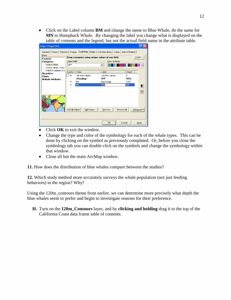
G. Turn-on and activate the Cascadall layer. Open the symbology tab and classify the whale data by species • Right-click on the Cascadall layer. • Select properties from the pop up menu. • In the Layer Properties Window select the symbology tab. • In the left side of the Window select the Categories option. • Select the Unique Values option. • In the Value field select the value SPP – this is the short hand used for species.

• Click the Add All Values from the bottom of the window. • Un-check the box next to <all other values>

12

• Click on the Label column BM and change the name to Blue Whale, do the same for MN to Humpback Whale. By changing the label you change what is displayed on the table of contents and the legend, but not the actual field name in the attribute table.

• Click OK to exit the window. • Change the type and color of the symbology for each of the whale types. This can be

done by clicking on the symbol as previously completed. Or, before you close the symbology tab you can double click on the symbols and change the symbology within that window.

• Close all but the main ArcMap window. 11. How does the distribution of blue whales compare between the studies? 12. Which study method more accurately surveys the whale population (not just feeding behaviors) in the region? Why? Using the 120m_contours theme from earlier, we can determine more precisely what depth the blue whales seem to prefer and begin to investigate reasons for their preference.

H. Turn on the 120m_Contours layer, and by clicking and holding drag it to the top of the

California Coast data frame table of contents.

13

I. Turn off the Cascadall layer

J. With the 120_contours layer active, use the identify tool ( ) to determine which contour line includes most of the blue whales. Make sure you zoom to the extent of the contours layers, don’t worry about the whale data outside of that extent. • With the Info tool and the 120m_countours layer active click on the contours that

appear to be closest to the majority of the blue whales points. You may need to zoom in and out to select the right contour.

13. At what depth do most of the blue whales congregate? Why might they be found here? Blue whales are filter feeders; they feed primarily on krill. During the WHAPS whale study, scientists found several different krill species (Tysanoessa spinifera, Euphausia pacifica and Nematosceles difficilis) congregated in slightly different areas in the study area. Dense layers of Tysanoessa spinifera were more common in shelf waters, less than 150 meters deep, while dense layers of Euphausia pacifica and Nematosceles difficilis were more common near or off the shelf edge in waters 200 meters deep.

K. Add the 150m_cont and 200m_cont layers. Adjust the color so they are easily visible against the bathymetry theme. • Both of these are steps that you’ve previously completed in this lab. If you need help

reference previous sections of this lab guide. 14. Based upon the distribution of whales in the WHAPS theme, which krill species do the blue whales seem to prefer? Why? How could you determine for certain which krill species blue whales prefer?

L. Turn on the Cascadall layer again and study the distribution of humpback whales. 15. Suggest reasons for the different distribution patterns between the blue whales and humpback whales.

14

The high concentration of krill species found off the north side of San Miguel, Santa Rosa and Santa Cruz islands is not a random event. All three krill species sampled are normally found in the colder waters of northern and central California. Between May - June, strong equatorial winds drive coastal upwelling off the coast of Point Conception. The upwelled waters enter the Santa Barbara Channel north of San Miguel moving eastward. The cold, nutrient-rich waters support large phytoplankton blooms which in turn support dense populations of zooplankton and small fish species. The large blue and humpback whales are attracted seasonally to the area to feed on the dense swarms. 16. Write a paragraph describing how the physical characteristics of an area can affect species distributions.

M. Take a screen shot of your map project, and paste it at the end of the Word document containing your answers to the questions in this lab.

N. Complete two of the three extension activities below (your choice) and include your answers to the

questions for those activities in your write-up.

15

Extension Activities (Complete your choice of 2 of 3 activities below) 1. Continue exploring the environmental sensitivity data provided. Which islands and species would be

affected the most by an oil spill? During which months would a spill be the most disastrous, impacting the largest number of species and interfering with breeding efforts?

2. Continue analyzing the WHAPS data. Analyze the distribution of each whale or dolphin species. How

are dolphins and porpoises distributed around the Sanctuary? Do they aggregate in any one part of the sanctuary? Suggest reasons for the different distribution patterns. Hint: Compare the eating habits of blue and humpback whales with dolphins and porpoises.

3. Create your own contour chart showing the bathymetry of the CINMS. Experiment with changing

the contour interval. Select contour intervals to show areas of safe SCUBA depth, shallow water productive areas, or other features of interest.

Open the explore Arc Map project you were previously working on. Activate the California Coast data frame if it is not already activated.

Turn off all layers except California.

Add the grid layer Bathy, if not already added, from your student directory/LAB_2/LAB_2_data,

Zoom to the extent of the Bathy layer

This layer will be at the bottom of the table on contents since it is a grid layer Turn on the Spatial Analyst Extension.

• Under the Tools menu in the main Arc Map menu bar select Extensions… • In the Extensions Window check the Spatial Analyst check box. • Close the Extensions Window.

Add the Spatial Analyst tool bar to Arc Map.

• In the main Arc Map menu bar click on View and select Toolbars… • Click on Spatial Analyst and the menu will close automatically, and the new tool bar

will docked at the top of Arc Map.

In the Spatial Analyst tool bar click on “Spatial Analyst” and scroll down to Surface Analysis and select Contour…

16

In the Contour Window make sure the input surface is set to Bathy, and that the contour interval is

50.

Save the new Contour file as 50m_contour in your student directory where you’ve previously saved your explore Arc Map Project.

Click OK in the Contour Window, it will take a few seconds and the computer calculates the new

contour file. The new 50m_contour layer will automatically be added to the top of your table on contents.

Turn off the Bathy layer, and zoom to the extent of the 50m_contour layer.

Take a screen shot, of your map project, and paste it at the end of the Word document containing

your answers to the questions in this lab.

Drop your entire write-up in the dropfolder or DropBox, make sure your name and lab# are in both the filename of the Word document as well as within the document itself