DPRIETI Discussion Paper Series 20-E-059

Overinvestment and Macroeconomic Uncertainty:Evidence from Renewable and Non-Renewable Resource Firms

IRAWAN, DennyAustralian National University

OKIMOTO, TatsuyoshiRIETI

The Research Institute of Economy, Trade and Industryhttps://www.rieti.go.jp/en/

1

RIETI Discussion Paper Series 20-E-059

June 2020

Overinvestment and Macroeconomic Uncertainty:

Evidence from Renewable and Non-Renewable Resource Firms*

Denny Irawan†a and Tatsuyoshi Okimoto‡a,b

ａCrawford School of Public Policy, Australian National University

b Research Institute of Economy, Trade and Industry (RIETI)

Abstract

Investment is an inherent component of business activities. This study examines the tendency of

resource firms to overinvest induced by the business cycle and uncertainties. The analysis is conducted

using unbalanced panel data drawn from 584 resource companies across 32 countries covering 1986

to 2017 in four resource sectors: (1) alternative energy, (2) forestry and paper, (3) mining, and (4) oil

and gas producers. The results indicate that the forestry and paper sector overinvests relative to the

standard investment level predicted by the investment function regardless of the sample period, while

the alternative energy sector tends to underinvest. Also, many emerging economies, including Brazil,

China, India, Indonesia, Russia, and South Korea, are found to have overinvested over the last three

decades or so. In addition, the results suggest that commodity price inflation plays a more important

role in inducing firms' overinvestment than commodity price uncertainty. It is also found that the home

country's business cycle significantly affects overinvestment, with the sign alternating from negative

to positive after the global financial crisis. Furthermore, the finding also shows no significant

relationship between global geopolitical risk and overinvestment but a significantly positive

relationship is found between global economic and country-level governance policy uncertainties and

overinvestment. Lastly, the results suggest that the effect of overinvestment on firm performance after

three years is positive, especially for firms in the mining sector.

Keywords: Overinvestment, Business Cycle, Uncertainty, Natural Resource Companies

JEL classification: E32, G30, G32

The RIETI Discussion Paper Series aims at widely disseminating research results in the form of professional

papers, with the goal of stimulating lively discussion. The views expressed in the papers are solely those of

the author(s), and neither represent those of the organization(s) to which the author(s) belong(s) nor the

Research Institute of Economy, Trade and Industry.

*A part of this study is a result of the research project at Research Institute of Economy, Trade and Industry (RIETI)

by the second author. The authors would like to thank Renee Fry-McKibbin, David Stern, Yixiao Zhou, Warwick

McKibbin, Quentin Grafton, Donald Winchester, Debasish Das, seminar participants at ANU and RIETI, and

participants of the 32nd Australasian Finance and Banking Conference (AFBC), for their valuable comments. †Ph.D. Scholar, Crawford School of Public Policy, Australian National University. Address: 132 Lennox Crossing,

ANU, Acton 2601, Australia. E-mail: denny.irawan@anu.edu.au. ‡ Associate Professor, Crawford School of Public Policy, Australian National University; and Visiting Fellow,

RIETI. Address: 132 Lennox Crossing, ANU, Acton 2601, Australia. E-mail: tatsuyoshi.okimoto@anu.edu.au.

1. Introduction

Investment is an inherent component of business activities. By making investments, firmsgrow their capacity to increase output. However, the important economic notion of optimal-ity also applies to firm investments. What if firms invest more than they should? Richardson(2006) defines this phenomenon as overinvestment. He proposes a relative measure that as-sesses the degree of over- and underinvestment using residuals from firms’ investment func-tions. Overinvestment can be considered as a result of firms’ risk taking behaviour, providinghigher firms’ performance sometimes but putting them in trouble other times. Therefore, ifmany firms in a sector or country overinvests, there may be too much risk for the sector orcountry. Thus, it is useful to identify the sectors and countries that tend to overinvest, aswell as the possible causes of this overinvestment. This study identifies overinvestment andits causes among resource companies from 32 G20-area countries.

Furthermore, it is also useful to assess how overinvestment affects firm performance.From the macroeconomic point of view, overinvestment could have both positive and nega-tive effects. When the business cycle is in a booming phase, general prices increase and thusinduce firms to invest more to increase their production capacities (Kiyotaki, 2011). On amassive scale, this can expand aggregate overinvestment in the economy, which would furtherboost the economy, at least in the short term. However, the overinvestment would have anadverse inter-temporal impact and damage the economy in the long term. Firm overinvest-ment could also have both negative and positive side effects from the microeconomic point ofview. For example, Kulatilaka and Perotti (1998), Weeds (1999), Chevalier-Roignant et al.(2011), and Henriques and Sadorsky (2011) suggest that increasing investment, which couldbe characterized as overinvestment, is a favourable strategy for firms under high uncertainty,as the overinvestment could improve their performance. On the other hand, Fu (2010), Liuand Bredin (2010), and Ling et al. (2016) argue that overinvesting has a significantly neg-ative impact on the future performance of firms. Therefore, it is worthwhile empiricallyassessing the effects of overinvestment on firm performance, which this study performs forresource companies across a number of major countries.

In 2017, the total natural resource exports from the sample countries accounted for1,566.43 billion USD. Russia and the United States are the world leaders in the export ofnatural resources, followed by other G20 countries, such as Australia, Saudi Arabia, Canada,and Brazil. Furthermore, the natural resource exports play the critical role in driving manyleading economies. Natural resource exports accounted for more than 50% of exports forSaudi Arabia, Russia, and Australia. For many other countries, natural resource exportsaccounted for more than 20% of their total exports (Brazil, Greece, Indonesia, Canada,South Africa, and Cyprus). Although the role of the resource sector in the overall economy(as a percentage of total value-added and total employment) might be decreasing, naturalresource exports still play a vital role in maintaining macroeconomic performance for thesecountries, primarily through the export channel. These facts emphasize the importance ofanalysing overinvestment in the resource sector, providing a solid reason to focus on thesector.

This study contributes to the literature by providing a comprehensive empirical explo-

2

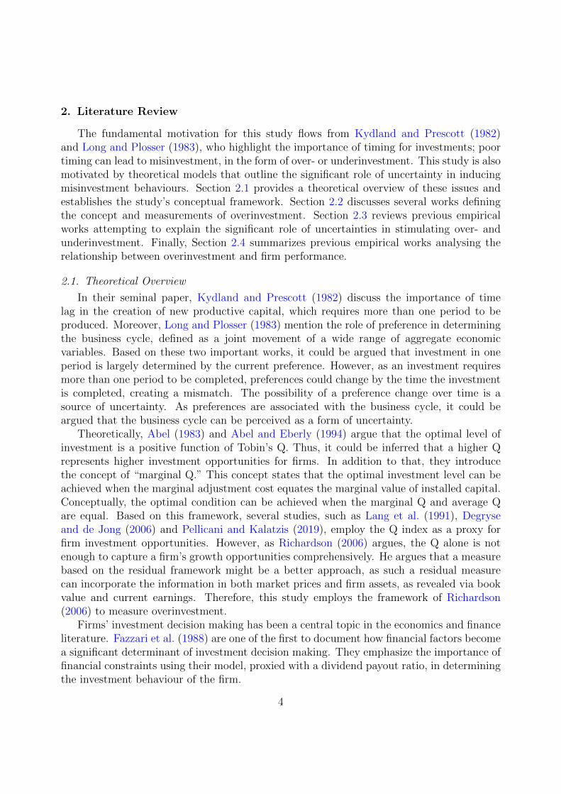
ration of overinvestment behaviour and its relation with business cycles and macroeconomicuncertainties among resource companies from 32 G20-area countries. Three analyses areconducted to clarify the characteristics of overinvestment and their effects on firm perfor-mance. First, this study examines overinvestment and underinvestment behaviour amongthe sample firms in each period using the framework developed by Richardson (2006). Sec-ond, this study examines whether business cycles and macroeconomic uncertainties play asignificant role in explaining overinvestment behaviour. Third, this study examines howoverinvestment affects firm performance.

This study considers the business cycle as a possible source of overinvestment. Specifi-cally, this study employs a dual business cycle approach by considering the world businesscycle and the home-country business cycle. This dual approach is effective in capturingthe overall effect of business cycle fluctuations on companies’ overinvestment behaviour. Inaddition, commodity price uncertainty, global geopolitical uncertainty, and global economicpolicy uncertainty are considered in order to examine the relationship between overinvest-ment and uncertainty. Furthermore, a worldwide governance indicator is adopted as a proxyfor country-level uncertainty.

This study offers several significant findings. The first analysis indicates that internalfirm factors play a significant role in determining firms’ investment decision making and thatthe 2008 global financial crisis had a significant impact on overinvestment patterns in manycountries. This result is also confirmed statistically by comparing estimated parameters fromthe investment function between before and after 2008. Also, the results suggest that theforestry and paper sector overinvests relative to the standard investment level predicted bythe investment function regardless of the sample period, while the alternative energy sectortends to underinvest. Furthermore, many emerging economies, including Brazil, China, In-dia, Indonesia, Russia, and South Korea, are found to overinvest over the last three decadesor so. The second analysis shows that commodity price inflation plays a more importantrole in inducing firms’ overinvestment than commodity price uncertainty does. The homecountry business cycle also significantly affects overinvestment, with signs alternating fromnegative to positive before and after the global financial crisis, while the world business cyclehas no significant relationship with overinvestment. The finding also shows no significantrelationship between global geopolitical risk and overinvestment but finds a significantly pos-itive relationship between global economic and country-level governance policy uncertaintiesand overinvestment. Finally, the third analysis demonstrates that the effect of overinvest-ment on firm performance is positive, especially for firms in the mining sector. This findingsupports Kulatilaka and Perotti (1998), Weeds (1999), Chevalier-Roignant et al. (2011),and Henriques and Sadorsky (2011), who suggest that overinvesting might be a favourablestrategy for firms facing uncertainty.

The remainder of the paper is structured as follows. Section 2 reviews the literature andprovides theoretical background on overinvestment and discusses the empirical literature onthe measurement of overinvestment and its relation to uncertainty and firm performance.Section 3 explains the study’s dataset, while Section 4 explains the study’s methodology.Section 5 presents the study’s empirical results and discusses them, focusing on their rele-vance to the literature. Finally, Section 6 concludes the paper.

3

2. Literature Review

The fundamental motivation for this study flows from Kydland and Prescott (1982)and Long and Plosser (1983), who highlight the importance of timing for investments; poortiming can lead to misinvestment, in the form of over- or underinvestment. This study is alsomotivated by theoretical models that outline the significant role of uncertainty in inducingmisinvestment behaviours. Section 2.1 provides a theoretical overview of these issues andestablishes the study’s conceptual framework. Section 2.2 discusses several works definingthe concept and measurements of overinvestment. Section 2.3 reviews previous empiricalworks attempting to explain the significant role of uncertainties in stimulating over- andunderinvestment. Finally, Section 2.4 summarizes previous empirical works analysing therelationship between overinvestment and firm performance.

2.1. Theoretical Overview

In their seminal paper, Kydland and Prescott (1982) discuss the importance of timelag in the creation of new productive capital, which requires more than one period to beproduced. Moreover, Long and Plosser (1983) mention the role of preference in determiningthe business cycle, defined as a joint movement of a wide range of aggregate economicvariables. Based on these two important works, it could be argued that investment in oneperiod is largely determined by the current preference. However, as an investment requiresmore than one period to be completed, preferences could change by the time the investmentis completed, creating a mismatch. The possibility of a preference change over time is asource of uncertainty. As preferences are associated with the business cycle, it could beargued that the business cycle can be perceived as a form of uncertainty.

Theoretically, Abel (1983) and Abel and Eberly (1994) argue that the optimal level ofinvestment is a positive function of Tobin’s Q. Thus, it could be inferred that a higher Qrepresents higher investment opportunities for firms. In addition to that, they introducethe concept of “marginal Q.” This concept states that the optimal investment level can beachieved when the marginal adjustment cost equates the marginal value of installed capital.Conceptually, the optimal condition can be achieved when the marginal Q and average Qare equal. Based on this framework, several studies, such as Lang et al. (1991), Degryseand de Jong (2006) and Pellicani and Kalatzis (2019), employ the Q index as a proxy forfirm investment opportunities. However, as Richardson (2006) argues, the Q alone is notenough to capture a firm’s growth opportunities comprehensively. He argues that a measurebased on the residual framework might be a better approach, as such a residual measurecan incorporate the information in both market prices and firm assets, as revealed via bookvalue and current earnings. Therefore, this study employs the framework of Richardson(2006) to measure overinvestment.

Firms’ investment decision making has been a central topic in the economics and financeliterature. Fazzari et al. (1988) are one of the first to document how financial factors becomea significant determinant of investment decision making. They emphasize the importance offinancial constraints using their model, proxied with a dividend payout ratio, in determiningthe investment behaviour of the firm.

4

Furthermore, Bebchuk and Stole (1993) discuss how uncertainty, in the form of imper-fect information and short-term managerial objectives, may boost firms’ overinvestment (orunderinvestment) tendencies. Their model predicts that overinvestment occurs when themarket observes the number of opportunities for investment but lacks complete informationregarding productivity, while underinvestment occurs when the market lacks complete in-formation regarding the number of opportunities for investment. Lorenzoni (2008) presentsa theoretical model of how uncertainty may cause an inefficient credit boom. He outlinesthe importance of financial friction in the form of revenue shocks, which may cause a firmto make inefficient investments and thus inefficient leverage decisions.

Glover and Levine (2015) provide dual theoretical predictions of how uncertainty canaffect firms’ investments. On the one hand, uncertainty may increase investment. Profitscan increase at an increasing rate if firms have a positive and convex relationship betweenprofit and cost or demand (i.e. if cost or demand increase). Furthermore, uncertainty maypositively increase investment if firms have the ability to reverse their investments. Thiscondition causes higher uncertainty increases the marginal utility of capital and thus in-vestments. This positive relationship is outlined by Oi (1961), Hartman (1972), and Abel(1983). On the other hand, some theoretical models predict a negative relationship betweenuncertainty and investment. The basis of this prediction is the presence of irreversibility,which may cause firms to delay investments when uncertainty is high. This negative relation-ship is supported by Bernanke (1983), Brennan and Schwartz (1985), McDonald and Siegel(1986), Pindyck (1988), and Dixit and Pindyck (1994). Thus, there are dual effects of uncer-tainty on investment depending on the assumptions of the framework. However, Glover andLevine (2015) also point out that most empirical works find a negative relationship betweenuncertainty and investment.

2.2. Overinvestment: Concept and Measurement

Attempts to explain firms’ overinvestment behaviours can be traced to Fazzari et al.(1988), who outline the role of financial constraint proxied by a dividend payout as a causeof overinvestment. Firms with a low payout ratio are identified as financially unconstrainedand as thus having a higher tendency to overinvest. Their model is supported by the empir-ical finding that firms with a low payout ratio have higher investment-cashflow sensitivity.Fazzari et al. (1988) is followed by other studies, such as Bond and Meghir (1994), Chap-man et al. (1996), Whited and Wu (2006), Almeida and Campello (2007), Carpenter andGuariglia (2008), and Wang et al. (2016), who use various proxies of financial constraint.

Richardson (2006) introduces an accounting-based framework to measure the overinvest-ment phenomenon. He defines overinvestment as a form of investment at an amount thatexceeds the normal or expected level given the firm’s characteristics and economic condi-tions. This definition can be considered an accounting-based definition of overinvestmentbecause, in this framework, overinvestment is measured based on firm-specific variables,such as value, leverage, cash availability, and age. The framework estimates the investmentfunction of all firms in the dataset in a panel setting, which generates an estimated pa-rameter for each explanatory variable. From these parameters, the fitted values are thenconstructed to represent the ideal amount of new investment for each firm. The residual

5

from this estimation is defined as the misinvestment, or, specifically, the unexplained partof the firms’ investment. The positive value of this residual represents overinvestment, whilethe negative value represents underinvestment. One major reason why this study choosesthe framework of Richardson (2006) is that it is among the most popular measures due toits straightforward and easy-to-compute characteristics; it requires only balance sheet infor-mation. Many studies adopt this framework for overinvestment analysis, such as Zhang andSu (2015), Guariglia and Yang (2016), Wei et al. (2019), and Yu et al. (2020).

In their framework, Richardson (2006) employ the ‘new investment’ spent by the firmas the dependent variable (INEW ). This variable is calculated as the current year’s totalinvestment expenditure subtracted by the total investment required to maintain existingassets. Thus, in this framework, the dependent variable is expressed as the amount of newinvestment, instead of the total investment stock inside the firm. The rationale for thischoice is that the analysis of overinvestment focuses on how a firm decides upon a new in-vestment within a certain business environment. Considering that the business environmentis dynamic, change in investment is considered better able to capture firm behaviour thantotal investment stock. Empirically, Richardson (2006) employs this framework to examinethe overinvestment phenomenon using 58,053 firm-year observations drawn from Compus-tat data on non-financial firms covering 1988 to 2002. The result shows that the averagefirm overinvests 20% of its available free cash flow. However, Bergstresser (2006) criticizesthis framework for being based on the residual of the model, which results in a zero-meancharacteristic and balanced observations of overinvestment and underinvestment.

2.3. Overinvestment and Uncertainty

Many studies have contributed to the literature on how firms’ external uncertainty playsa vital role in explaining the overinvestment tendency. Proost and Van Der Loo (2010)develop a theoretical model to identify the role of demand uncertainty in overinvestmentand underinvestment for transport infrastructure. They find that an overinvesting actionis costly in the presence of demand uncertainty. Henriques and Sadorsky (2011) empiri-cally examine the effect of oil price uncertainty on strategic investment. Although theirapproach does not directly analyse the relationship between oil price uncertainty and theoverinvestment phenomenon, their results suggest a U-shaped relationship between oil pricevolatility and firm-level investment. In other words, when oil price uncertainty is high, firmsshould increase investments, which can be characterized as overinvestment, suggesting thatoverinvestment could be beneficial for firms in high-uncertainty circumstances.

Dixit and Pindyck (1994) provide a very rigorous discussion about investment underuncertainty, which emphasizes the role of irreversibility, uncertainty, and timing in invest-ment decision making. This concept motivates many empirical works, such as Bloom (2009)and Sha et al. (2020), to examine the investment decision making process. However, theempirical works conducted by these studies are only focused on firms in a specific country.Bloom (2009) implements the analysis using US firms data, meanwhile Sha et al. (2020) fo-cus on Chinese firms’ data. Furthermore, these studies focus on investment decision-makingand do not specifically discuss the dynamics of over- and underinvestment. These two factsdistinguish their study with the analysis conducted in this study.

6

Chevalier-Roignant et al. (2011) provide a comprehensive literature review on firms’strategic investment and conclude that overinvesting seems favourable amid increased un-certainty. Their review include models developed by Kulatilaka and Perotti (1998) andWeeds (1999). Weeds (1999) argues that economic and technological uncertainty might in-duce a firm to invest in technology that they will leave unexploited, known as the ‘sleepingpatent,’ in order to retain their position as a dominant firm and block new entrants. Mean-while, Kulatilaka and Perotti (1998), motivated by Dixit (1980) and in line with Spence(1979), develop a model of strategic investment under high uncertainty and competition.Their model indicates that an overinvesting action is favourable under many conditions,even under increased volatility. This conclusion is based on their argument that increaseduncertainty provides more opportunity rather than just simply higher risk. One importantthing to note from these studies is that they focus on strategic aspects such as industrystructure and the market share where firms operate. Those factors are, therefore, impor-tant for overinvestment analysis. However, those factors are most feasible to be analyzedwhen estimation focuses on firms in a specific country or region. To this extent, this study,which focuses on resource companies from around the world, can hardly accommodate thesestrategic aspects to the analysis. Yet, the insights provided by this literature regarding thepositive relationship pattern between uncertainty and overinvestment are very crucial forthe analysis conducted in this study.

Another model by Heikkinen and Pietola (2009) suggests that uncertainty increases theoverinvestment tendency. Wang et al. (2016) empirically examine how inflation uncertaintycan lower the tendency to overinvest. Liu (2013) identifies the vital role of policy uncer-tainty, which contributes to overinvestment in wind power capacity in China. Ahuja andNovelli (2017) argue that increased uncertainty can lead to research and development (R&D)overinvestment in a firm due to the complexity of investment decision making, especially inlarge companies with many divisions.

Yoon and Ratti (2011) show that energy prices play a vital role in determining firminvestment stability. Drakos and Goulas (2006) outline the positive response of investmenttoward uncertainty. By contrast, Acharya and Sadath (2016) and Caballero (1991) find anegative relationship between energy price uncertainty and firm investments. Ma (2016)argues that there is no significant effect of GDP uncertainty on investment. Ghosal andLoungani (2000) and Gulen and Ion (2016) also report a negative investment-uncertaintyrelationship.

Based on these studies, it could be argued that the relationship between uncertaintyand investment is indeterminate, although some studies, such as Kulatilaka and Perotti(1998), Weeds (1999), Chevalier-Roignant et al. (2011), and Henriques and Sadorsky (2011)suggest that overinvestment might be a favourable strategy for firms amid uncertainty. Thisstudy contributes to this strand of literature by empirically examining how economic andnon-economic macro uncertainties affect resource companies’ tendency to overinvest.

2.4. Overinvestment and Performance

Several studies investigate the relationship between overinvestment and firm perfor-mance. For example, Kulatilaka and Perotti (1998), Weeds (1999), Chevalier-Roignant et al.

7

(2011), and Henriques and Sadorsky (2011) suggest that, amid high uncertainty, increasinginvestments, which could be characterized as overinvestment, might improve firm perfor-mance. On the other hand, Fu (2010) examines the relationship between overinvestmentand the operating performance of seasoned equity offering companies (SEOs) and showsthat overinvestment is significant in explaining firms’ poor performance. Likewise, Liu andBredin (2010) investigate the role of institutional investors in inducing firms’ overinvestmentand examine how overinvestment might affect corporate performance. They report a sig-nificantly negative relation between overinvestment and corporate performance. Moreover,Ling et al. (2016) examine the relationship between political connections and overinvest-ment and explore how both factors influence firm performance. They find that firms withpolitical connections have a higher tendency to overinvest and that this condition lowersfirm performance. Thus, it could be argued that overinvestment has a mixed relationshipwith firm performance.

3. Data

This study examines the overinvestment phenomenon at the firm level. A firm is cate-gorized as overinvesting if its investment level is considered to be higher than its predictedlevel from the firm’s investment function, which is estimated in a panel setting. The proxyof investment is calculated as the difference of total capital divided by the average of totalassets, following the framework of Richardson (2006). The analysis uses 7,984 firm-year ob-servations drawn from 584 natural resource companies from 32 countries in the G20 area.3

The dataset is unbalanced, and the regression analysis covers the 32 years spanning 1986 to2017. The analysis are limited to companies with at least 10 years of observations withouta gap. Detailed information regarding the number of observations and companies for eachsector is provided in Table 1.

[Table 1]

There are four resource sectors in the analysis, which follow the Worldscope Datastreamclassification: (1) alternative energy,4 (2) forestry and paper, (3) mining, and (4) oil andgas producers. Companies in these four sectors are grouped into two broad classificationsbased on their resource characteristics: renewable and non-renewable. The renewable groupis comprised of alternative energy and forestry and paper companies. The non-renewablegroup is comprised of mining and oil and gas production companies. Nevertheless, it isacknowledged that some companies in the dataset might involve in more than one business

3There are more than 20 countries in the G20 because the European Union (EU) is counted as onemember, except for some of the EU’s most industrialized countries (Germany, France and Italy), whichare also present alone. Observations from firms in the European Union are included to accommodate thissituation. If Hong Kong is counted as a single country, the dataset comprises 33 countries.

4The alternative energy sector comprises firms which are either (1) manufacturers of renewable energyequipment such as wind turbines and solar panels; or (2) producers of biofuels. Thus, most firms in thissector are manufacturing firms.

8

activities, which may include both renewable and non-renewable businesses. The WorldscopeDatastream classifies each company based on their primary business activity, and thereforethis study follows that classification to group them into renewable and non-renewable. Thisstudy acknowledges this condition as a caveat of the dataset.

On the one hand, conducting an analysis in a cross-country setting makes the datasetprone to the cross-country heteroscedasticity problem. On the other hand, one of the maincharacteristics of resource companies is they operate across countries to expand and topursue the resources they are seeking. This is particularly true of non-renewable companies,which dominate the dataset. Therefore, the analysis is conducted in a cross-country settingwith country-level macroeconomic variables used as controls.

The balance sheet data of the sample companies are acquired from Worldscope Datas-tream. Seven main variables are employed in this study: (1) total assets, (2) total capital,5

(3) total shareholders’ equity, (4) total debt, (5) cash, (6) market capitalization, and (7)operating income.6 Firm age is proxied by the current year subtracted by the first yearin the data available from the Worldscope database. The data are in annual frequency,primarily based on the end-of-year balance sheet position. All companies are publicly listedand are limited to companies categorized as major, primary quote, and active based on theWorldscope classification. The data are acquired in the local currency in which the firmis listed. Most firm-level variables are normalized with the average of total assets or aretransformed into a logarithmic scale.

The dataset also includes macroeconomic data, at both the world and country levels. Atthe world level, commodity price data—specifically, the Goldman Sachs Commodity Index(GSCI)—is applied. This commodity price index is one of the most popular commodityindexes in the financial market. The GSCI is based on future contracts, which representcurrent market expectations of future conditions. The index is in daily frequency, andthe annual average of the daily data is used as the proxy for the commodity price cycle.The index also proxies for price uncertainty, using the annual standard deviation of thedaily GSCI. This study also employs the global Geopolitical Risk index (GEOPOL) fromCaldara and Iacoviello (2018) and the Global Economic Policy Uncertainty index (GEPU)from Davis (2016) as proxies of global uncertainty. A higher GEOPOL and GEPU indicateshigher uncertainty. Data for GEOPOL and GEPU are provided and updated monthly bythe authors on the associated websites.7

At the country level, the study uses GDP growth, inflation rate, and the WorldwideGovernance Indicators (WGI) of the World Bank. The WGI index plays a vital role as a

5Specifically, total capital represents total investment in the company, which is calculated as the sumof common equity, preferred stock, minority interest, long-term debt, non-equity reserves, and deferred taxliability in untaxed reserves.

6The following are codes for each variable acquired from Worldscope Datastream: (1) total assets -WC02999, (2) total capital - WC03998, (3) total shareholders’ equity - WC03995, (4) total debt - WC03255,(5) cash - WC02003, (6) market capitalization - WC08001, and (7) operating income - WC01250.

7Data for GEOPOL are provided by Caldara and Iacoviello (2018) on https://www.matteoiacoviello.

com/gpr.htm. Data for GEPU are provided by Davis (2016) on https://www.policyuncertainty.com/

global_monthly.html.

9

proxy for country-level uncertainty. The study uses the average of six categories: (1) voiceand accountability, (2) political stability and the absence of violence/terrorism, (3) govern-ment effectiveness, (4) regulatory quality, (5) the rule of law, and (6) control of corruption.The WGI ranges from -2.5 to 2.5, where a higher value indicates better governance. Thisvalue is inverted by multiplying -1 to take the opposite, with a higher value indicating poorgovernance, for ease of analysis.

As shown by the GSCI index, there is a strong indication of a structural break in thecommodity price in 2008 (see Figure 1). This indication is also confirmed by the supremumWald test conducted to track structural break with an unknown break date as in Casiniand Perron (2019). The test is implemented to daily GSCI data based on the 2nd orderautoregressive (AR(2)) model and suggests a structural break on July 7, 2008.8 The resultis reported in Table 2. Based on this stylized fact, the analysis is conducted for three periods:(1) the full period of 1986-2017; (2) before 2008, including 1986 to 2007; and (3) after 2008,including 2009 to 2017. The year 2008 is excluded in the sub-period analysis because it isthe exact year when the anomaly and structural break occurred.

[Figure 1]

[Table 2]

It is fully acknowledged that some, if not most, of the companies in the observationoperate in a multinational setting, and most are export-oriented. Therefore, the homecountry’s business cycle should not be the only proxy used for the business cycle. Thisstudy also employs the global business cycle, represented by global annual GDP growth.This dual business cycle approach is effective in capturing the overall effect of business cyclefluctuation on companies’ investment behaviours.

The dataset initially contained outliers reflecting extreme economic phenomena, such asBrazilian hyperinflation in the early 1990s, which could affect the dataset’s overall statisticaldistribution. Some companies also had extreme balance sheet profiles, such as extremenegative equity, which could distort the overall statistical properties of the dataset. Thus,these outliers were eliminated. The elimination process was conducted in two steps. Firstly,outliers were eliminated, especially on leverage (LEV ) and inflation (INFL) data, as thesetwo variables were identified as being the most prone to the outlier problem. The datasetwas trimmed one percent in the upper and lower percentile based on these two variables.Secondly, after the outliers were removed, companies were limited to which have at least10 years of observations without a gap. Descriptive statistics of the final dataset and thecorrelations between variables are presented in Tables 3 and 4.

[Table 3]

[Table 4]

8The lag 2 is chosen based on Akaike Information Criterion (AIC) and Hannan–Quinn InformationCriterion (HQIC).

10

4. Methodology

4.1. Overinvestment

Overinvestment is proxied by the positive residuals of the firm investment function,based on the firm’s specific variables. The specification used to measure overinvestment wasdeveloped by Richardson (2006) and has been implemented in several studies, such as Zhangand Su (2015), Guariglia and Yang (2016), Wei et al. (2019), and Yu et al. (2020). Theequation for the firm investment function is as follows:

(1)INV Ti,t = β0 + β1V/P i,t−1 + β2LEV i,t−1 + β3CASH i,t−1 + β4SIZEi,t−1

+ β5RTRN i,t−1 + β6INV T i,t−1 + β7AGEi,t−1 + ΣY RID + ΣFRID + µi,t

where the subscript i = 1, 2, ..., i denotes firm in the sample, meanwhile t denotes year. Theterm INV T reflects the investment of the firm i at time t, calculated as the change in totalcapital divided by the average of total assets. This term is similar to the new investmentvariable used by Richardson (2006). The term V/P is a proxy of a firm’s growth opportunity,which is the ratio between the firm’s book value of shareholders’ equity divided by marketcapitalization. The term LEV reflects the leverage ratio, calculated as total debt dividedby the average of total assets. The term CASH is the firm’s total cash divided by theaverage of total assets. The term SIZE is the log-transformation of total assets. The termRTRN is the firm’s annual return, calculated as the annual growth of the firm’s marketcapitalization. The term AGE is firm age, calculated as the current year subtracted bythe first year for which data are available in the Worldscope database, as indicated by the‘History/Hist’ column in the firm’s profile. The term Y RID is the year fixed effect dummy.The term FRID is the firms’ fixed effect dummy. The error term µ in this equation is aproxy for firm misinvestment; a positive value indicates overinvestment, while a negativevalue indicates underinvestment. Equation (1) is estimated using the panel fixed-effectordinary least squares (OLS) with clustered error specification, where the firm is the cluster.All regressors are one-year lagged to avoid the endogeneity problem, following Richardson(2006). As there are 21 panels for each analysis, there are 21 µ in this study, specificallyµm,n, where m = 1, ..., 3 denotes estimation period, meanwhile n = 1, ..., 7 denotes sampleset (see Table 9).

Furthermore, this study also conducts joint and separate Chow tests to check parametersstability from estimation (1).9 The test is conducted by estimating joint equations andmultiplying each independent variable with dummy indexes referring to before and after2008, excluding the year 2008. After that, joint and separate F tests are implemented to seewhether parameters from before 2008 are statistically different with parameters from after2008. If they are statistically different, thus it could be inferred that a structural breakhappened. The joint F test is conducted to see whether parameters from each estimationbefore 2008 are jointly and statistically different from its counterpart after 2008. Meanwhile,the separate F test is aimed to see the stability of each parameter between before and after2008.

9For more details please see (Greene, 2018, pp. 191).

11

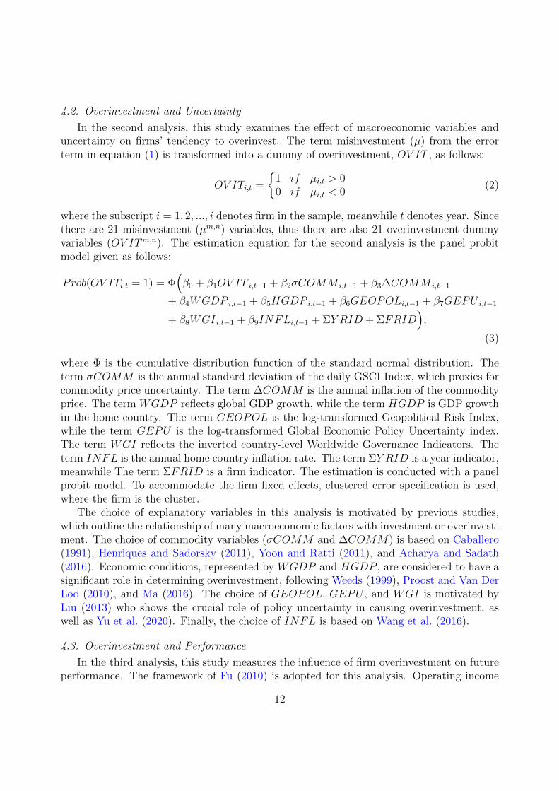
4.2. Overinvestment and Uncertainty

In the second analysis, this study examines the effect of macroeconomic variables anduncertainty on firms’ tendency to overinvest. The term misinvestment (µ) from the errorterm in equation (1) is transformed into a dummy of overinvestment, OV IT , as follows:

(2)OV ITi,t =

{1 if µi,t > 00 if µi,t < 0

where the subscript i = 1, 2, ..., i denotes firm in the sample, meanwhile t denotes year. Sincethere are 21 misinvestment (µm,n) variables, thus there are also 21 overinvestment dummyvariables (OV ITm,n). The estimation equation for the second analysis is the panel probitmodel given as follows:

Prob(OV ITi,t = 1) = Φ(β0 + β1OV IT i,t−1 + β2σCOMM i,t−1 + β3∆COMM i,t−1

+ β4WGDP i,t−1 + β5HGDP i,t−1 + β6GEOPOLi,t−1 + β7GEPU i,t−1

+ β8WGI i,t−1 + β9INFLi,t−1 + ΣY RID + ΣFRID),

(3)

where Φ is the cumulative distribution function of the standard normal distribution. Theterm σCOMM is the annual standard deviation of the daily GSCI Index, which proxies forcommodity price uncertainty. The term ∆COMM is the annual inflation of the commodityprice. The term WGDP reflects global GDP growth, while the term HGDP is GDP growthin the home country. The term GEOPOL is the log-transformed Geopolitical Risk Index,while the term GEPU is the log-transformed Global Economic Policy Uncertainty index.The term WGI reflects the inverted country-level Worldwide Governance Indicators. Theterm INFL is the annual home country inflation rate. The term ΣY RID is a year indicator,meanwhile The term ΣFRID is a firm indicator. The estimation is conducted with a panelprobit model. To accommodate the firm fixed effects, clustered error specification is used,where the firm is the cluster.

The choice of explanatory variables in this analysis is motivated by previous studies,which outline the relationship of many macroeconomic factors with investment or overinvest-ment. The choice of commodity variables (σCOMM and ∆COMM) is based on Caballero(1991), Henriques and Sadorsky (2011), Yoon and Ratti (2011), and Acharya and Sadath(2016). Economic conditions, represented by WGDP and HGDP , are considered to have asignificant role in determining overinvestment, following Weeds (1999), Proost and Van DerLoo (2010), and Ma (2016). The choice of GEOPOL, GEPU , and WGI is motivated byLiu (2013) who shows the crucial role of policy uncertainty in causing overinvestment, aswell as Yu et al. (2020). Finally, the choice of INFL is based on Wang et al. (2016).

4.3. Overinvestment and Performance

In the third analysis, this study measures the influence of firm overinvestment on futureperformance. The framework of Fu (2010) is adopted for this analysis. Operating income

12

divided by the average of assets, ROA, is employed as the dependent variable because thistype of ROA represents income from real business activities conducted by a company ratherthan from investing or financing activities.

Three-year lags are implemented for the investment variables (INV T , OV IT , andINV T ∗OV IT ) in this analysis due to the time lag between the disbursement of money forinvestments and the moment when the investment begins to operate. The three-year lags areused as a benchmark following Topp et al. (2008), who outline that the average constructiontime for mining (including oil and gas) projects is 2.1 years. The average construction timefor new mining developments is 2.4 years, and the average time required for mine expansionis 1.7 years. A one-year lag is implemented for other firm-level control variables.

The estimation equation for performance is as follows:

(4)

ROAi,t = β0 + β1INV Ti,t−1 + β2OV ITi,t−1 + β3INV Ti,t−1 ∗OV ITi,t−1+ β4INV Ti,t−2 + β5OV ITi,t−2 + β6INV Ti,t−2 ∗OV ITi,t−2+ β7INV Ti,t−3 + β8OV ITi,t−3 + β9INV Ti,t−3 ∗OV ITi,t−3 + β10V/Ai,t−1+ β11ROAi,t−1 + β12SIZEi,t−1 + ΣY RID + ΣFRID + ei,t

where the subscript i = 1, 2, ..., i denotes firm in the sample, meanwhile t denotes year. Theterm ROA represents company performance, as represented by operating income dividedby average assets. The term INV T is company investment, represented by the change in afirm’s total capital divided by average total assets. The term OV IT is the overinvestmentdummy, and the term INV T ∗ OV IT is an interaction term for company investment andoverinvestment. The term V/A represents firms’ market capitalization divided by averageassets, and the term SIZE is the log-transformation of a firm’s total assets. The term eis an error term. The estimation is conducted with panel fixed-effect OLS, with the fixedeffect applied at the firm level.

5. Empirical Results

This section presents the empirical results. For each analysis, estimations are conductedusing the full dataset and at a disaggregated level by sector for the three sample periods:the full period, before 2008, and after 2008. For ease of presentation, the results of the yearand firm fixed effects are excluded.

5.1. Overinvestment

The first analysis is based on a firm’s investment function (1). The dependent variableof this regression is INV T , and all regressors are firm-specific variables following specifi-cations from Richardson (2006). The equation is estimated using panel fixed-effect OLS,with the year and firm fixed effects. This means that each analysis is regressed in a panelsetting, following Richardson (2006) and many other studies that also implement the sameframework. One major difference is that Richardson (2006) implements the fixed effects atthe industry level because his analysis focuses on companies in one country with multiplesectors. By contrast, this study focuses on companies from many countries with different

13

characteristics. Therefore, this study implements the fixed effects at the firm level. Thismeans that all companies are regressed in one fixed effects panel. They have exactly thesame set of parameters, but each firm has a specific effect that comes from the firm-levelfixed effects. Therefore, the residuals (the misinvestments) for each firm are comparablewith those of other firms and can be aggregated. The estimation results are presented inTables 5-7.

[Table 5]

[Table 6]

[Table 7]

As can be seen from the tables, the coefficient on V/P is significant and stable witha negative sign for most regressions, suggesting that overvalued firms have a tendency toinvest more. The coefficient on LEV is estimated to be highly significantly negative forseveral panels in the post-2008 period. The negative sign indicates that firms tend to investless once they have already leveraged. This finding is logical because leveraging is a majoroption for firms to finance investments. These results are fairly consistent with those ofRichardson (2006).

The coefficient on CASH is found to be significantly positive in the post-2008 periodonly for the forestry and paper panel. Thus, in contrast to those in Richardson (2006), theseresults show that cash level is not a major determinant of firms’ investments before 2008.In addition, the significantly positive estimates after 2008 might suggest that firms withmore cash are more aggressive and invest more after the global financial crisis, especially forforestry and paper firms.

The coefficient on SIZE is found to be significantly negative for all panels and periods,indicating that large firms have lower investment rates. Meanwhile, the coefficient on RTRNis estimated to be significantly positive for most of the cases. At least from the market pointof view, RTRN could be considered a proxy for overall firm performance, meaning that thebetter a firm has performed in the previous year, the higher its tendency to invest.

[Table 8]

Furthermore, joint and separate Chow tests are conducted to compare estimated param-eters from Table 6 and Table 7. This test aims to see whether parameters from before andafter 2008 estimations are statistically different. The joint Chow test focuses on the jointstability of the parameters between before and after 2008. Meanwhile, the separate Chowtest focuses on the stability of each parameter. To conduct this test, each estimation inTable 6 is merged with it’s counterpart in Table 7 and jointly estimated as one equation,with each variable is indexed with a dummy indicating the period of before and after 2008(b2008 and a2008). The results of both joint and separate tests are presented in Table 8.Based on the value of the F test, it can be seen whether parameters from before 2008 arestatistically different after 2008. The joint test results show that parameters from all panels

14

are jointly different between before and after 2008 based on the F value, strongly suggestinga structural break in all estimations.

Results for separate Chow tests suggest that many coefficients are not stable, especiallyfor non-renewable companies (Table 8). Specifically, the coefficient on the variable INV T isnot stable for the alternative energy, forestry paper, and mining panels. The coefficient onV/P is not stable for the full sample, non-renewable, and mining; meanwhile, the coefficienton LEV is not stable in the full sample, non-renewable, and oil and gas panels. Thecoefficient on CASH is found stable for all panels; meanwhile, for SIZE, the coefficientis only found stable for the alternative energy panel. Lastly, the coefficient on RTRN isfound not stable for the alternative energy and mining panels; meanwhile, the coefficienton AGE is found not stable for the renewable, alternative energy, and oil and gas panels.In general, these results outline that the stability of each parameter between before andafter 2008 varies significantly based on the sub-sample. Therefore, the results from thefull sample estimation, although they are correct, are not sufficient to describe the overallcharacteristics of the firms in the sample. This fact shows the importance of dividing theanalysis into several sub-samples. In addition, the results also suggest a strong indication ofa major structural break for non-renewable companies, as shown by the number of non-stablecoefficients for the mining and oil and gas panels.

[Table 9]

The residuals, or the variable misinvestment (µ), are obtained in each estimation inthe first analysis. The variable µ describes the degree of firm over- and underinvestmentcompared to its predicted value from the investment function. There are 21 misinvestmentvariables, µ, from the 21 panels of the analysis (see Table 9). Each µ is indexed as µm,n wherem = 1, ..., 3 refers to period and n = 1, ..., 7 refers to sample set. For ease of presentation,only the results of µ1,1, which are residuals from the full period-full sample estimation, arepresented. A statistical description of µ1,1 by sector is presented in Table 10. The morepositive the value of µ1,1, the higher the overinvestment; the more negative the value of µ1,1,the greater the underinvestment. Specifically, in Table 10, µ1,1 are divided into sectors andtime periods to show the pattern variations. Furthermore, over- and underinvestment levelsare classified into three categories based on the mean value of µ1,1:

(5)

Degree of misinvestment

=

{ overinvestment if mean ≥ 0.05 → dark gray shadeneutral if −0.05 < mean < 0.05 → white shade

underinvestment if mean ≤ −0.05 → light gray shade

As can be seen in Table 10, regardless of the sample period, the alternative energy sectorunderinvests relative to the standard investment level predicted by the investment function(1). This result could suggest that renewable energy development may be underdevelopedcompared to the conventional energy sector because the oil and gas production sector isclassified as neutral in the results.

15

[Table 10]

By contrast, Table 10 demonstrates that the forestry and paper sector overinvests re-gardless of the sample period, suggesting that the forestry and paper sector generally hasan investment rate higher than the standard investment level predicted by the investmentfunction (1). This sector is comprised mostly of forestry and paper mill companies. Thehigh investment rate in this sector might provide insight into the demand growth for paperproducts. However, on the upstream side of this industry, a higher investment rate mightbe seen to indicate a higher rate of conversion from natural to industrial forest.

The mining sector has an underinvestment pattern in the full period. However, aninteresting pattern change for this sector occurs from neutral before 2008 to underinvestingafter 2008. The results indicate that a structural break occurs in the investment patternin the mining sector before and after the 2008 financial crisis. Investment in this sector isobserved to be highly conservative after the crisis.

For the oil and gas producer sector, the investment pattern is stable in the neutralposition for all three sample periods, indicating the stability of the proper investment ratein this sector.

Furthermore, µ1,1 is also plotted according to the market, as can be seen in Figures 2-4and is statistically summarised by Table 11. For most markets, the misinvestment patternremains the same before and after 2008 (Table 11). Particularly, many emerging economies,including Brazil, China, India, Indonesia, Russia, and South Korea, are found to overinvestover the last three decades or so. The exceptions are Belgium, Canada, Germany, andPoland, which changed from neutral before 2008 to underinvesting after 2008. A similardownward pattern can be observed for Finland, Portugal, and Spain, which changed fromoverinvesting before 2008 to neutral after 2008. For others, upward patterns can be observed,such as for Hong Kong SAR, Romania, and Turkey, where the pattern changed from neutralbefore 2008 to overinvesting after 2008. The change in the pattern of overinvestment foreach market appears to be determined by market-specific factors, especially those relatedto macroeconomic conditions before and after 2008. Some markets may have experienced along period of extensive investment before 2008, which was then corrected when the 2008crisis occurred.

[Table 11]

[Figure 2]

[Figure 3]

[Figure 4]

This study is among the first to analyse overinvestment patterns in resource sectors usingthe Richardson (2006)’s method, conducted at the firm level in a cross-country setting. Inthe next subsection, this study examines whether macroeconomic factors and uncertaintiescan explain the investment patterns of the sample firms.

16

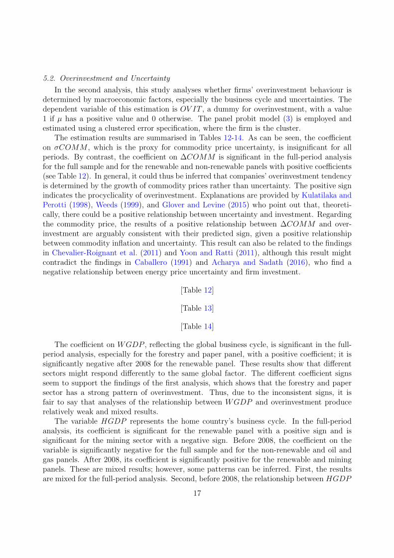
5.2. Overinvestment and Uncertainty

In the second analysis, this study analyses whether firms’ overinvestment behaviour isdetermined by macroeconomic factors, especially the business cycle and uncertainties. Thedependent variable of this estimation is OV IT , a dummy for overinvestment, with a value1 if µ has a positive value and 0 otherwise. The panel probit model (3) is employed andestimated using a clustered error specification, where the firm is the cluster.

The estimation results are summarised in Tables 12-14. As can be seen, the coefficienton σCOMM , which is the proxy for commodity price uncertainty, is insignificant for allperiods. By contrast, the coefficient on ∆COMM is significant in the full-period analysisfor the full sample and for the renewable and non-renewable panels with positive coefficients(see Table 12). In general, it could thus be inferred that companies’ overinvestment tendencyis determined by the growth of commodity prices rather than uncertainty. The positive signindicates the procyclicality of overinvestment. Explanations are provided by Kulatilaka andPerotti (1998), Weeds (1999), and Glover and Levine (2015) who point out that, theoreti-cally, there could be a positive relationship between uncertainty and investment. Regardingthe commodity price, the results of a positive relationship between ∆COMM and over-investment are arguably consistent with their predicted sign, given a positive relationshipbetween commodity inflation and uncertainty. This result can also be related to the findingsin Chevalier-Roignant et al. (2011) and Yoon and Ratti (2011), although this result mightcontradict the findings in Caballero (1991) and Acharya and Sadath (2016), who find anegative relationship between energy price uncertainty and firm investment.

[Table 12]

[Table 13]

[Table 14]

The coefficient on WGDP , reflecting the global business cycle, is significant in the full-period analysis, especially for the forestry and paper panel, with a positive coefficient; it issignificantly negative after 2008 for the renewable panel. These results show that differentsectors might respond differently to the same global factor. The different coefficient signsseem to support the findings of the first analysis, which shows that the forestry and papersector has a strong pattern of overinvestment. Thus, due to the inconsistent signs, it isfair to say that analyses of the relationship between WGDP and overinvestment producerelatively weak and mixed results.

The variable HGDP represents the home country’s business cycle. In the full-periodanalysis, its coefficient is significant for the renewable panel with a positive sign and issignificant for the mining sector with a negative sign. Before 2008, the coefficient on thevariable is significantly negative for the full sample and for the non-renewable and oil andgas panels. After 2008, its coefficient is significantly positive for the renewable and miningpanels. These are mixed results; however, some patterns can be inferred. First, the resultsare mixed for the full-period analysis. Second, before 2008, the relationship between HGDP

17

and overinvestment is negative. Third, after 2008, the relationship between HGDP andoverinvestment is positive. The change in pattern from negative to positive before and after2008 could be caused by the global financial crisis, which also changed the behaviour ofcompanies in the sample. Moreover, comparing the results for WGDP and HGDP suggeststhat the home country’s business cycle (HGDP ) plays a more important role in affectingthe overinvestment behaviour of resource firms than WGDP does. The mixed results onthe relationship between the business cycle and overinvestment might be slightly differentfrom those of Ma (2016), who finds no significant relationship between GDP uncertaintyand investment.

The next variable of interest is the Geopolitical Risk Index (GEOPOL), which representsglobal geopolitical instability. The index is a scalar measure, wherein a higher value indicateshigher uncertainty. For the full-period analysis, the coefficient on GEOPOL is significantlypositive only for the renewable and alternative energy panels. However, before 2008, itscoefficient is significantly negative only for the full-sample panel. Given these results, itcould be inferred that GEOPOL and overinvestment do not have a significant relationship.

The variable GEPU plays a vital role as a measure of global economic policy uncertainty.For the full-period analysis, the coefficient of this variable is significant for the full sampleand for the renewable and forestry and paper panels with positive signs. In general, thisvariable is not significant for the non-renewable sectors, such as the mining and oil and gasproduction sectors. Therefore, it could be inferred that global economic policy uncertaintyhas a positive relationship with overinvestment, especially for the renewable sector.

The next variable is WGI, which is a proxy for country-level non-economic uncertainty.The inverted version of this index is applied for ease of analysis; a higher number indicatespoor governance. As can be seen from Tables 12-14, the coefficient on WGI is statisti-cally significant for all panels in all periods with positive signs. Thus, there is a clear andstrong pattern wherein poor governance at the country level has a positive relationship withoverinvestment.

The positive relationship of GEPU and WGI with overinvestment supports the findingsof many previous studies, such as Drakos and Goulas (2006), Heikkinen and Pietola (2009),Liu (2013), Glover and Levine (2015), and Ahuja and Novelli (2017). These studies find apositive relationship between uncertainty and firm overinvestment or investment. The resultsalso support Kulatilaka and Perotti (1998), Weeds (1999), Chevalier-Roignant et al. (2011),and Henriques and Sadorsky (2011), who suggest that overinvesting might be a favourablestrategy for firms facing uncertainty. However, the findings contradict Ghosal and Loungani(2000) and Gulen and Ion (2016), who report a negative investment-uncertainty relationship.

In general, the country-level control variable, inflation (INFL), is found to be signifi-cantly negative, especially for the full period and after 2008. These results are in line withthose of Wang et al. (2016), who find that inflation uncertainty reduces overinvestmenttendencies, given a positive correlation between inflation and inflation uncertainty.

5.3. Overinvestment and Performance

In the third analysis, this study examines the relationship between overinvestment andfirms’ future performance based on Equation (4). The framework of Fu (2010) is used to

18

measure the effect. One- to three-year lags are employed for the investment-related variables(INV T , OV IT , and INV T ∗OV IT ), following the benchmark used by Topp et al. (2008),who outline the average construction time for mining projects. The dependent variable isoperating income divided by the average of assets (operating ROA), which represents theincome surge from the firms’ main business activities. The analysis is divided into the fullsample and the sub-sample panels and the full period and sub-periods, as in the previousanalyses. Equation (4) is estimated using panel fixed-effect OLS, where the fixed effect isimplemented at the firm level. The estimation results are presented in Tables 15-17.

[Table 15]

[Table 16]

[Table 17]

The coefficient of INV Tt−2 and INV Tt−3 are found to be significantly negative for thefull sample and for the non-renewable and mining panels in the full period and the post-2008 period. These results indicate that, in non-renewable sectors, investments will generallyreduce future performance, especially after the 2008 global financial crisis.

The coefficient on OV IT , the overinvestment dummy, is generally found to be not sig-nificant, although it is either positive or negative for several specific lags and sample esti-mations. It could thus be inferred that there is no conclusive relationship between OV ITas a standalone variable and firms’ future performance.

However, the results for the interaction term INV T ∗ OV IT indicate that it has agenerally positive relationship with future performance, especially for the lag-three in the fullsample and for the non-renewable and mining panels in the full-period and post-2008-periodanalysis. Any interpretation of the results for the interaction term should consider the resultsof the main term INV T , which is generally negative. Thus, INV T has a generally negativerelationship with future firm performance. For overinvesting firms, however, the joint effect(INV T ∗OV IT ) will be positive. It could thus be inferred that overinvesting might have apositive impact on firms’ future performance, especially for firms in the mining sector. Theseresults support those of Kulatilaka and Perotti (1998), Weeds (1999), Chevalier-Roignantet al. (2011), and Henriques and Sadorsky (2011), who suggest that overinvesting might bea favourable strategy for firms facing uncertainty. On the other hand, the results contradictthe findings of Fu (2010), Liu and Bredin (2010), and Ling et al. (2016), who find thatoverinvestment has a significantly negative impact on future performance.

It could also be inferred that the most significant relationship between the investment-related variables (INV T , OV IT , and INV T ∗ OV IT ) and performance exists in the lag-three. This finding highlights the importance of the time lapse between investment andperformance, as outlined by Kydland and Prescott (1982). The finding also supports Toppet al. (2008), who find that the construction time for mining projects might span between1.7 to 2.4 years. Thus, this study confirms the delayed impact of investment on firm perfor-mance.

19

6. Conclusion

This study has examined the tendency of resource firms to overinvest induced by thebusiness cycle and macroeconomic uncertainties. The analysis has been conducted usingunbalanced panel data drawn from 584 resource companies across 32 countries spanning1986 to 2017 in four resource sectors: (1) alternative energy, (2) forestry and paper, (3)mining, and (4) oil and gas production. The analysis was also conducted by grouping thefirst two sectors as renewable, and the other two as non-renewable. This grouping hasprovided interesting insights into overinvestment behavior between the renewable and non-renewable firms.

Three analyses have been conducted to clarify the role the business cycle and uncertaintyplay in overinvestment and its effects on firm performance. First, the overinvestment andunderinvestment behaviours of each firm in the sample have been investigated using theframework developed by Richardson (2006). The results indicated that internal firm factorsplay a significant role in determining firms’ investment decision making. The results alsosuggested that the 2008 global financial crisis had a significant impact on overinvestmentpatterns in many countries. The separate Chow test results showed that many coefficientsof non-renewable companies are not stable, which strongly suggested that a structural breakoccurred in 2008 for the mining and oil and gas sectors. Also, the results confirmed that theforestry and paper sector overinvests relative to the standard investment level predicted bythe investment function regardless of the sample period, while the alternative energy sectortends to underinvest. Furthermore, many emerging economies, including Brazil, China,India, Indonesia, Russia, and South Korea, were found to overinvest over the last threedecades or so.

Second, this study has examined whether the business cycle and uncertainty play a sig-nificant role in explaining firms’ overinvestment behaviour. The study found a significantlypositive relationship between commodity price inflation and overinvestment and found noclear relationship between commodity price uncertainty and overinvestment. In addition,the results showed that although the global business cycle has no noticeable relationshipwith overinvestment, the home country’s business cycle significantly affects overinvestment,with signs alternating from negative to positive before and after the global financial crisis.Furthermore, the study found no significant relationship between global geopolitical risk andoverinvestment but found a significantly positive relationship between global economic andcountry-level governance policy uncertainties and overinvestment.

Finally, the study has explored how overinvestment may affect firms’ future performance.The results demonstrated that the joint effect of investment and overinvestment is positivefor firm performance, especially for firms in the mining sector. These results support Kulati-laka and Perotti (1998), Weeds (1999), Chevalier-Roignant et al. (2011), and Henriques andSadorsky (2011), who suggest that overinvesting might be a favourable strategy for firmsfacing uncertainty. A further extension from this study should consider the inclusion ofstrategic factors in the market where firms operate, such as industry structure and marketshare, following formal models discussed by Kulatilaka and Perotti (1998), Weeds (1999),Chevalier-Roignant et al. (2011), and Henriques and Sadorsky (2011).

20

References

Abel, A. B. (1983). Optimal investment under uncertainty. American Economic Review, 73(1):228–233.Abel, A. B. and Eberly, J. C. (1994). A Unified Model of Investment Under Uncertainty. American Economic

Review, 84(5):1369–1384.Acharya, H. R. and Sadath, C. A. (2016). Energy Price Uncertainty and Investment: Firm Level Evidence

from Indian Manufacturing Sector. International Journal of Energy Economics and Policy, 6(3):364–373.Ahuja, G. and Novelli, E. (2017). Activity Overinvestment: The Case of R&D. Journal of Management,

43(8):2456–2468.Almeida, H. and Campello, M. (2007). Financial Constraints, Asset Tangibility, and Corporate Investment.

Review of Financial Studies, 20(5):1429–1460.Bebchuk, L. A. and Stole, L. A. (1993). Do Short-Term Objectives Lead to Under- or Overinvestment in

Long-Term Projects? The Journal of Finance, 48(2):719–729.Bergstresser, D. (2006). Discussion of “Overinvestment of free cash flow”. Review of Accounting Studies,

11(2-3):191–202.Bernanke, B. S. (1983). Irreversibility, Uncertainty, and Cyclical Investment. The Quarterly Journal of

Economics, 98(1):85.Bloom, N. (2009). The Impact of Uncertainty Shocks. Econometrica, 77(3):623–685.Bond, S. and Meghir, C. (1994). Dynamic Investment Models and the Firm’s Financial Policy. The Review

of Economic Studies, 61(2):197–222.Brennan, M. J. and Schwartz, E. S. (1985). Evaluating Natural Resource Investments. The Journal of

Business, 58:135–157.Caballero, R. J. (1991). On the Sign of the Investment-Uncertainty Relationship. American Economic

Review, 81(1):279–288.Caldara, D. and Iacoviello, M. (2018). Measuring Geopolitical Risk. International Finance Discussion

Paper, 2018(1222):1–66.Carpenter, R. E. and Guariglia, A. (2008). Cash flow, investment, and investment opportunities: New tests

using UK panel data. Journal of Banking & Finance, 32(9):1894–1906.Casini, A. and Perron, P. (2019). Structural Breaks in Time Series. In Oxford Research Encyclopedia of

Economics and Finance. Oxford University Press.Chapman, D. R., Junor, C. W., and Stegman, T. R. (1996). Cash flow constraints and firms’ investment

behaviour. Applied Economics, 28(8):1037–1044.Chevalier-Roignant, B., Flath, C. M., Huchzermeier, A., and Trigeorgis, L. (2011). Strategic investment

under uncertainty: A synthesis. European Journal of Operational Research, 215(3):639–650.Davis, S. J. (2016). An Index of Global Economic Policy Uncertainty. NBER Working Paper, (October):1–

12.Degryse, H. and de Jong, A. (2006). Investment and internal finance: Asymmetric information or managerial

discretion? International Journal of Industrial Organization, 24(1):125–147.Dixit, A. (1980). The Role of Investment in Entry-Deterrence. The Economic Journal, 90(357):95.Dixit, A. K. and Pindyck, R. S. (1994). Investment under Uncertainty. Princeton University Press.Drakos, K. and Goulas, E. (2006). Investment and conditional uncertainty: The role of market power,

irreversibility, and returns-to-scale. Economics Letters, 93(2):169–175.Fazzari, S. M., Hubbard, R. G., Petersen, B. C., Blinder, A. S., and Poterba, J. M. (1988). Financing

Constraints and Corporate Investment. Brookings Papers on Economic Activity, 1988(1):141.Fu, F. (2010). Overinvestment and the Operating Performance of SEO Firms. Financial Management,

39:249–272.Ghosal, V. and Loungani, P. (2000). The Differential Impact of Uncertainty on Investment in Small and

Large Businesses. Review of Economics and Statistics, 82(2):338–343.Glover, B. and Levine, O. (2015). Uncertainty, investment, and managerial incentives. Journal of Monetary

Economics, 69:121–137.Greene, W. (2018). Econometric Analysis. Pearson, New York, 8th edition.

21

Guariglia, A. and Yang, J. (2016). A balancing act: Managing financial constraints and agency costs tominimize investment inefficiency in the Chinese market. Journal of Corporate Finance, 36:111–130.

Gulen, H. and Ion, M. (2016). Policy Uncertainty and Corporate Investment. Review of Financial Studies,29(3):523–564.

Hartman, R. (1972). The effects of price and cost uncertainty on investment. Journal of Economic Theory,5(2):258–266.

Heikkinen, T. and Pietola, K. (2009). Investment and the dynamic cost of income uncertainty: The case ofdiminishing expectations in agriculture. European Journal of Operational Research, 192(2):634–646.

Henriques, I. and Sadorsky, P. (2011). The effect of oil price volatility on strategic investment. EnergyEconomics, 33(1):79–87.

Kiyotaki, N. (2011). A perspective on modern business cycle theory. Economic Quarterly, 97(3):195–208.Kulatilaka, N. and Perotti, E. C. (1998). Strategic Growth Options. Management Science, 44(8):1021–1031.Kydland, F. E. and Prescott, E. C. (1982). Time to Build and Aggregate Fluctuations. Econometrica,

50(6):1345–1370.Lang, L. H., Stulz, R., and Walkling, R. A. (1991). A test of the free cash flow hypothesis. Journal of

Financial Economics, 29(2):315–335.Ling, L., Zhou, X., Liang, Q., Song, P., and Zeng, H. (2016). Political connections, overinvestments and

firm performance: Evidence from Chinese listed real estate firms. Finance Research Letters, 18:328–333.Liu, N. and Bredin, D. (2010). Institutional Investors, Over-investment and Corporate Performance.Liu, X. (2013). The value of holding scarce wind resource—A cause of overinvestment in wind power capacity

in China. Energy Policy, 63:97–100.Long, J. B. and Plosser, C. I. (1983). Real Business Cycles. Journal of Political Economy, 91(1):39–69.Lorenzoni, G. (2008). Inefficient credit booms. Review of Economic Studies, 75(3):809–833.Ma, Y. (2016). Uncertainty and investment dynamics in the Australian mining industry. University of

Wollongong Thesis Collection 1954-2016.McDonald, R. and Siegel, D. (1986). The Value of Waiting to Invest. The Quarterly Journal of Economics,

101(4):707.Oi, W. Y. (1961). The Desirability of Price Instability Under Perfect Competition. Econometrica, 29(1):58.Pellicani, A. D. and Kalatzis, A. E. G. (2019). Ownership structure, overinvestment and underinvestment:

Evidence from Brazil. Research in International Business and Finance, 48:475–482.Pindyck, R. S. (1988). Irreversible Investment, Capacity Choice, and the Value of the Firm.Proost, S. and Van Der Loo, S. (2010). Transport infrastructure investment and demand uncertainty.

Journal of Intelligent Transportation Systems: Technology, Planning, and Operations, 14(3):129–139.Richardson, S. (2006). Over-investment of free cash flow. Review of Accounting Studies, 11(2-3):159–189.Sha, Y., Kang, C., and Wang, Z. (2020). Economic policy uncertainty and mergers and acquisitions:

Evidence from China. Economic Modelling.Spence, A. M. (1979). Investment Strategy and Growth in a New Market. The Bell Journal of Economics,

10(1):1.Topp, V., Soames, L., Parham, D., and Bloch, H. (2008). Productivity in the Mining Industry: Measurement

and Interpretation. Productivity Commission Staff Working Paper.Wang, Y., Chen, C. R., Chen, L., and Huang, Y. S. (2016). Overinvestment, inflation uncertainty, and

managerial overconfidence: Firm level analysis of Chinese corporations. North American Journal ofEconomics and Finance, 38:54–69.

Weeds, H. (1999). Sleeping patents and compulsory licensing: an options analysis. University of WarwickEconomic Research Papers.

Wei, X., Wang, C., and Guo, Y. (2019). Does quasi-mandatory dividend rule restrain overinvestment?International Review of Economics and Finance, 63:4–23.

Whited, T. M. and Wu, G. (2006). Financial constraints risk. Review of Financial Studies, 19(2):531–559.Yoon, K. H. and Ratti, R. A. (2011). Energy price uncertainty, energy intensity and firm investment. Energy

Economics, 33(1):67–78.Yu, X., Yao, Y., Zheng, H., and Zhang, L. (2020). The role of political connection on overinvestment of

22

Chinese energy firms. Energy Economics, 85:104516.Zhang, H. and Su, Z. (2015). Does media governance restrict corporate overinvestment behavior? Evidence

from Chinese listed firms. China Journal of Accounting Research, 8(1):41–57.

7. Appendix: Figures

Figure 1: Goldman Sachs Commodity Index (GSCI), 1970-2019

Source: Refinitiv Datastream

23

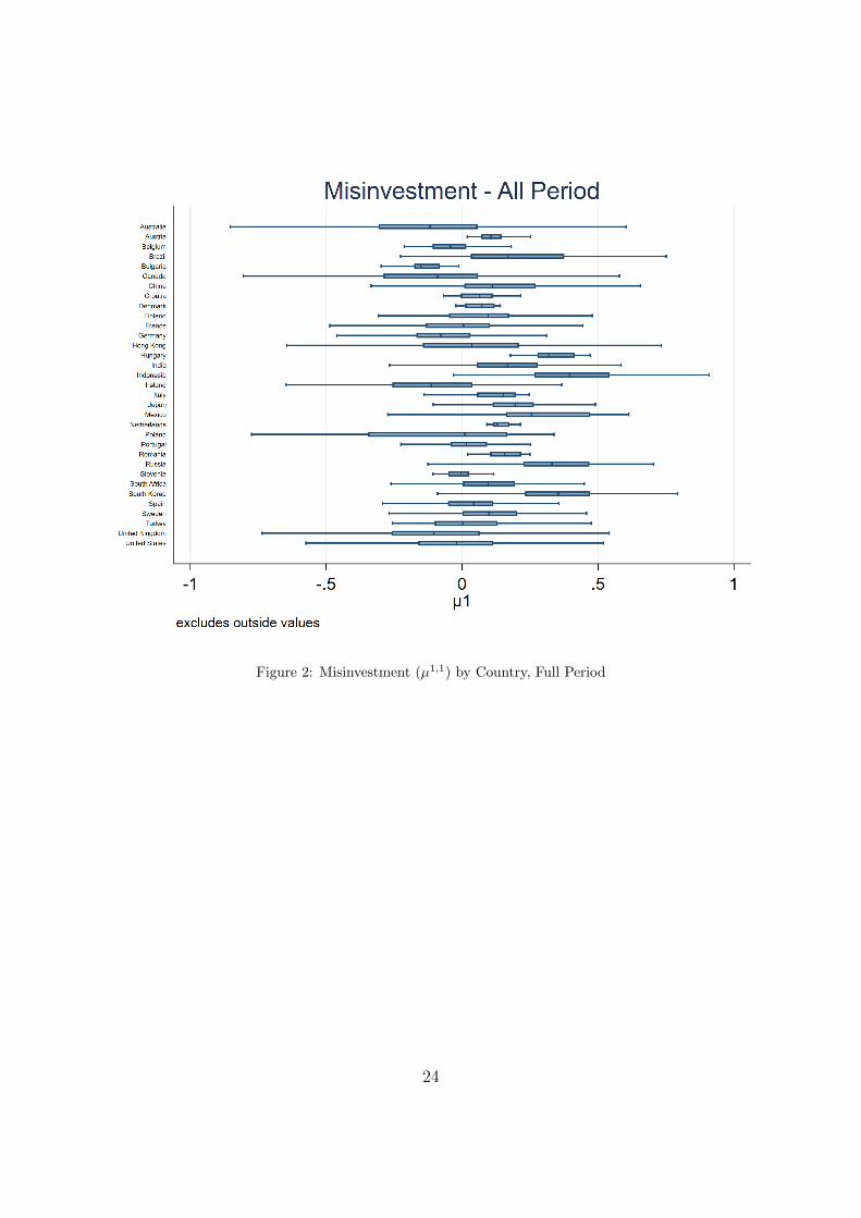
Figure 2: Misinvestment (µ1,1) by Country, Full Period

24

Figure 3: Misinvestment (µ1,1) by Country, Before 2008

25

Figure 4: Misinvestment (µ1,1) by Country, After 2008

26

8. Appendix: Tables

Table 1: Coverage of Sectors

No Sector Number of Companies Number of Observations1 Alternative Energy 40 4962 Forestry and Paper 86 1,4533 Mining 314 4,0434 Oil and Gas Producers 144 1,992

Total 584 7,984

Table 2: Result of Supremum Wald Test for Structural Break of the GSCI Index

Number of observations 12,839Full sample 02-Jan-1970 to 20-Mar-2019Trimmed sample 23-May-1977 to 02-Nov-2011Estimated break date 07-Jul-2008

H0: No Structural BreakTest Statistic p-valueSupremum Wald 110.4044 0.0000

Table 3: Descriptive Statistics

Variables Transformation Obs Mean Std. Dev. Min Max Source

INV T Capitalt−Capitalt−1

Assett7,984 0.0506 0.3335 -2.6053 2.4341 Worldscope

ROA Operating Income / Average of Assets 7,984 0.0075 0.1535 -0.9193 0.7114 WorldscopeV/A Market Capitalization / Average of Assets 7,984 1.0509 1.0823 0.0059 7.7618 WorldscopeV/P Equity / Market Capitalization 7,984 1.0313 1.0050 -3.6183 7.7908 WorldscopeLEV Total Liabilities / Total Assets 7,984 0.1946 0.2094 0.0000 2.7806 WorldscopeCASH Total Cash / Total Assets 7,984 0.1036 0.1469 -0.0041 1.0000 WorldscopeSIZE Natural Log of Total Assets 7,984 13.7262 3.9067 2.3026 25.3637 WorldscopeRTRN Growth of Market Capitalization (%) 7,984 0.3321 1.1544 -0.9706 12.0027 WorldscopeAGE Age - No Transformation 7,984 16.2885 9.7335 2.0000 53.0000 WorldscopeσCOMM Natural Log of Std Dev of Goldman Sachs Commodity Index 7,984 5.7327 0.7265 3.8070 7.5786 Datastream∆COMM Difference of Natural Log of Goldman Sachs Commodity Index 7,984 -0.6783 22.2911 -48.2286 50.9073 DatastreamWGDP Annual Growth of the World Economy 7,984 2.7784 1.4585 -1.6866 4.6170 World BankHGDP Annual Growth of the Home Country GDP 7,978 2.8112 2.6313 -8.2690 25.1173 World BankINFL Percentage - No Transformation 7,984 2.6448 2.2583 -4.4781 14.1108 World BankGEOPOL Geopolitical Risk (Global) - Natural Log Transformed 7,984 4.3889 0.3805 3.5000 5.3152 Caldara and Iacoviello (2018)GEPU Economic Policy Uncertainty (Global) - Natural Log Transformed 7,498 4.7209 0.3086 4.1356 5.2376 Davis (2016)WGI Worldwide Governance Index (Country) - Inverted 7,570 -1.1783 0.6742 -1.9700 0.9100 World Bank

Note: Total capital (World Scope WC03998) represents total investment in the company; which is calculatedas the sum of common equity, preferred stock, minority interest, long-term debt, non-equity reserves anddeferred tax liability in untaxed reserves.

27

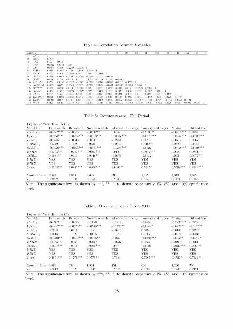
Table 4: Correlation Between Variables

Variables (1) (2) (3) (4) (5) (6) (7) (8) (9) (10) (11) (12) (13) (14) (15) (16) (17)(1) INV T 1(2) ROA 0.1793 1(3) V/A 0.312 0.0107 1(4) V/P -0.0862 -0.0363 -0.392 1(5) LEV -0.0676 0.1208 -0.2259 -0.0418 1(6) CASH 0.0316 -0.1966 0.1232 -0.1576 -0.1945 1(7) SIZE 0.0752 0.4904 -0.0696 0.0874 0.3898 -0.2989 1(8) RTRN 0.2277 -0.0072 0.2424 -0.2599 -0.0678 0.1522 -0.0728 1(9) AGE -0.0255 0.1767 0.0618 0.0111 0.1255 -0.1196 0.2579 -0.0905 1(10) σCOMM 0.0762 -0.0186 -0.0332 -0.0462 -0.0588 0.0476 -0.0582 -0.0213 -0.1721 1(11) ∆COMM 0.0903 0.0656 -0.0165 -0.0811 -0.0292 0.0145 -0.0097 -0.0206 -0.0895 0.2408 1(12) WGDP 0.0693 0.0291 0.0413 -0.0908 0.003 0.0231 0.0166 0.0532 0.013 -0.0699 0.6095 1(13) HGDP 0.0342 0.1036 -0.0079 -0.0287 0.0771 -0.0309 0.1981 0.0073 -0.113 -0.0091 0.3057 0.4701 1(14) INFL 0.0744 0.1599 -0.0031 0.0421 0.0581 -0.082 0.2493 0.0021 -0.117 0.2 0.2194 0.075 0.3082 1(15) GEOPOL -0.063 -0.0089 -0.0628 0.0376 0.0593 0.0022 0.0015 0.0108 0.1089 -0.1941 -0.0849 0.1216 0.0678 -0.1107 1(16) GEPU -0.0294 0.0068 0.1001 0.1374 0.0312 -0.0369 0.0366 -0.1055 0.1862 -0.5067 -0.1952 -0.2689 -0.1707 -0.0369 0.1121 1(17) WGI 0.0226 0.2745 -0.0716 0.04 0.2493 -0.1515 0.5847 -0.0115 -0.0763 -0.0056 -0.0097 -0.0091 0.4529 0.581 0.0002 0.0177 1

Table 5: Overinvestment - Full Period

Dependent Variable = INV TtVariables Full Sample Renewable Non-Renewable Alternative Energy Forestry and Paper Mining Oil and GasINV Tt−1 -0.0552*** -0.0883 -0.0512** 0.0344 -0.2090** -0.0816*** 0.0234V/Pt−1 -0.0778*** -0.0424*** -0.0928*** -0.0967*** -0.0279*** -0.0947*** -0.0903***LEVt−1 -0.0445 -0.0143 -0.0511 -0.2451 0.0026 -0.0717 0.0067CASHt−1 0.0379 0.1588 0.0135 -0.0912 0.4468** 0.0622 -0.0949SIZEt−1 -0.0426*** -0.0696*** -0.0431*** -0.1286*** -0.0322 -0.0358*** -0.0608***RTRNt−1 0.0205*** 0.0282*** 0.0162*** 0.0121 0.0377*** 0.0084 0.0341***AGEt−1 0.0031** 0.0013 0.0046** -0.0476 -0.0012 0.003 0.0077***Y RID YES YES YES YES YES YES YESFRID YES YES YES YES YES YES YESCons 0.6368*** 1.0863*** 0.6206*** 2.6002** 0.5515* 0.5598*** 0.8143***

Observations 7,984 1,949 6,035 496 1,453 4,043 1,992R2 0.0952 0.1099 0.1053 0.2383 0.1148 0.1171 0.1155

Note: The significance level is shown by ***, **, *, to denote respectively 1%, 5%, and 10% significancelevel.

Table 6: Overinvestment - Before 2008

Dependent Variable = INV TtVariables Full Sample Renewable Non-Renewable Alternative Energy Forestry and Paper Mining Oil and GasINV Tt−1 -0.0992 -0.0475 -0.1186 -0.1814 -0.025 -0.2830*** 0.2378V/Pt−1 -0.0487*** -0.0373** -0.0548*** -0.1120** -0.0242* -0.0278** -0.1315**LEVt−1 0.0908 0.0916 0.1157 -0.0215 0.0298 -0.0101 0.3333*CASHt−1 0.0016 0.1327 -0.0156 0.1675 0.1087 -0.0079 -0.0431SIZEt−1 -0.0313** -0.0552*** -0.0406** -0.076 -0.0431*** -0.0366* -0.0519*RTRNt−1 0.0153** 0.0067 0.0165* -0.0237 0.0234 0.0190* 0.0161AGEt−1 0.0064*** 0.0016 0.0102*** 0.047 -0.0001 0.0132*** 0.0063**Y RID YES YES YES YES YES YES YESFRID YES YES YES YES YES YES YESCons 0.4854*** 0.8779*** 0.5575** 0.7624 0.7167*** 0.4722* 0.7623**

Observations 2,803 839 1,964 151 688 1,260 704R2 0.0913 0.1027 0.1147 0.3446 0.1092 0.1346 0.2471

Note: The significance level is shown by ***, **, *, to denote respectively 1%, 5%, and 10% significancelevel.

28

Table 7: Overinvestment - After 2008

Dependent Variable = INV TtVariables Full Sample Renewable Non-Renewable Alternative Energy Forestry and Paper Mining Oil and GasINV Tt−1 -0.0568** -0.1569* -0.0470* 0.0506 -0.2718*** -0.0758*** 0.0192V/Pt−1 -0.0804*** -0.0393*** -0.0971*** -0.0762*** -0.0204* -0.1027*** -0.0843***LEVt−1 -0.1102** -0.1109 -0.1284** -0.3028* 0.0487 -0.1190** -0.1562CASHt−1 0.0572 0.2199 0.0342 -0.0021 0.6969* 0.1218 -0.1802SIZEt−1 -0.1322*** -0.1756*** -0.1273*** -0.1567*** -0.2119*** -0.1114*** -0.1662***RTRNt−1 0.0112 0.0329** 0.0037 0.0176 0.0434* -0.0073 0.0257AGEt−1 0.0068** -0.0067 0.0122*** -0.0052 -0.0034 0.0154*** 0.0081Y RID YES YES YES YES YES YES YESFRID YES YES YES YES YES YES YESCons 1.8001*** 2.9475*** 1.5882*** 2.2834*** 3.5972*** 1.2722*** 2.3657***

Observations 4,679 1,000 3,679 311 689 2,513 1,166R2 0.1276 0.1519 0.1362 0.1834 0.2025 0.1524 0.137

Note: The significance level is shown by ***, **, *, to denote respectively 1%, 5%, and 10% significancelevel.

Table 8: Chow Test of Parameter Estimates in Table 6 and Table 7

F − TestHypothesis Full Sample Renewable Non-Renewable Alternative Energy Forestry and Paper Mining Oil and Gas

Joint H0F(8, 6427) F(8, 1586) F(8, 4800) F(8, 361) F(8, 1186) F(8, 3180) F(8, 1579)5.95*** 2.73*** 8.02*** 3.68*** 1.99*** 7.68*** 3.86***

Sep

arat

eH

0

INV Tt−1,b2008 = INV Tt−1,a2008 0.44 0.97 0.70 3.24* 2.77* 5.28** 2.06V/Pt−1,b2008 = V/Pt−1,a2008 5.58** 0.01 4.26** 0.46 0.06 18.28*** 0.81LEVt−1,b2008 = LEVt−1,a2008 5.05** 1.29 4.90** 1.38 0.01 1.54 4.12**

CASHt−1,b2008 = CASHt−1,a2008 0.34 0.21 0.23 0.25 2.19 1.16 0.56SIZEt−1,b2008 = SIZEt−1,a2008 24.75*** 5.18** 14.00*** 1.45 3.34* 8.13*** 7.27***RTRNt−1,b2008 = RTRNt−1,a2008 0.17 2.61 1.23 3.23* 0.63 3.9** 0.23AGEt−1,b2008 = AGEt−1,a2008 1.46 3.08* 0.29 4.06** 2.59 1.04 3.79*

Consb2008 = Consa2008 0.81 0.00 0.70 3.77* 0.02 1.26 6.65**

Note: This table presents F value of joint and separate Chow test for coefficients from each estimation inTable 6 compared to its counterpart in Table 7. The subscript b2008 refers to before 2008 period, meanwhilea2008 refers to after 2008 period. The significance level is shown by ***, **, *, to denote respectively 1%,5%, and 10% significance level.

Table 9: The 21 Misinvestment Variables

µm,n Full Sample Renewable Non-Renewable Alternative Energy Forestry and Paper Mining Oil and Gas(1) (2) (3) (4) (5) (6) (7)

(1) Full Period µ1,1 µ1,2 µ1,3 µ1,4 µ1,5 µ1,6 µ1,7

(2) Before 2008 µ2,1 µ2,2 µ2,3 µ2,4 µ2,5 µ2,6 µ2,7

(3) After 2008 µ3,1 µ3,2 µ3,3 µ3,4 µ3,5 µ3,6 µ3,7

Note: Each µ represents misinvestment (residuals) from one investment panel analysis. It is indexed as µm,n

where m = 1, ..., 3 refers to period and n = 1, ..., 7 refers to sample set.

29

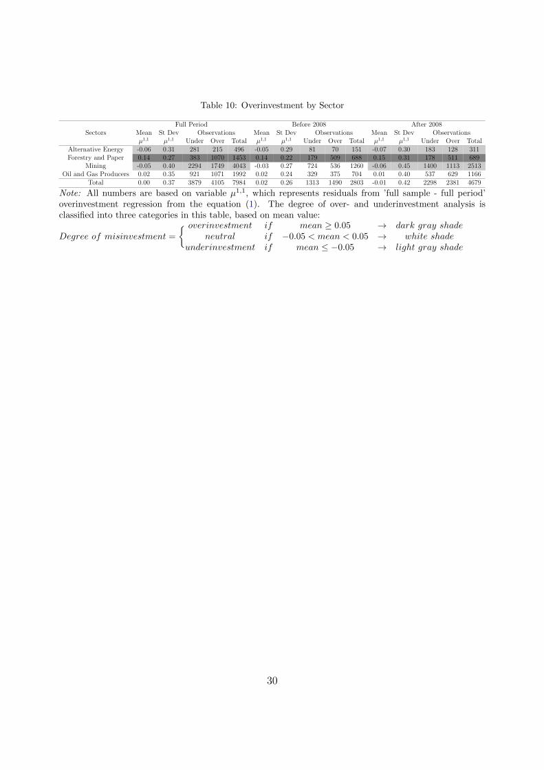
Table 10: Overinvestment by Sector

SectorsFull Period Before 2008 After 2008

Mean St Dev Observations Mean St Dev Observations Mean St Dev Observationsµ1,1 µ1,1 Under Over Total µ1,1 µ1,1 Under Over Total µ1,1 µ1,1 Under Over Total

Alternative Energy -0.06 0.31 281 215 496 -0.05 0.29 81 70 151 -0.07 0.30 183 128 311Forestry and Paper 0.14 0.27 383 1070 1453 0.14 0.22 179 509 688 0.15 0.31 178 511 689

Mining -0.05 0.40 2294 1749 4043 -0.03 0.27 724 536 1260 -0.06 0.45 1400 1113 2513Oil and Gas Producers 0.02 0.35 921 1071 1992 0.02 0.24 329 375 704 0.01 0.40 537 629 1166

Total 0.00 0.37 3879 4105 7984 0.02 0.26 1313 1490 2803 -0.01 0.42 2298 2381 4679

Note: All numbers are based on variable µ1,1, which represents residuals from ’full sample - full period’overinvestment regression from the equation (1). The degree of over- and underinvestment analysis isclassified into three categories in this table, based on mean value:

Degree of misinvestment =

{ overinvestment if mean ≥ 0.05 → dark gray shadeneutral if −0.05 < mean < 0.05 → white shade

underinvestment if mean ≤ −0.05 → light gray shade

30

Table 11: Overinvestment by Sector

No CountryFull Period Before 2008 After 2008

Mean St Dev Observations Mean St Dev Observations Mean St Dev Observationsµ1,1 µ1,1 Under Over Total µ1,1 µ1,1 Under Over Total µ1,1 µ1,1 Under Over Total

1 Australia -0.13 0.42 1190 574 1764 -0.11 0.29 467 171 638 -0.14 0.48 646 362 10082 Austria 0.12 0.07 0 29 29 0.11 0.07 0 19 19 0.15 0.08 0 9 93 Belgium -0.03 0.09 18 9 27 -0.01 0.07 9 8 17 -0.08 0.11 8 1 94 Brazil 0.21 0.25 6 27 33 0.21 0.08 0 3 3 0.23 0.26 5 22 275 Bulgaria -0.10 0.16 19 2 21 -0.16 0.00 1 0 1 -0.10 0.17 16 2 186 Canada -0.12 0.41 828 434 1262 -0.02 0.26 148 125 273 -0.14 0.44 615 283 8987 China 0.14 0.21 57 194 251 0.05 0.10 21 43 64 0.19 0.23 28 143 1718 Croatia 0.06 0.09 3 7 10 0.00 0.00 0 0 0 0.06 0.09 3 6 99 Denmark 0.11 0.14 2 16 18 0.09 0.10 1 7 8 0.12 0.18 1 8 9

10 Finland 0.08 0.25 29 47 76 0.14 0.27 12 39 51 -0.03 0.13 14 7 2111 France -0.01 0.20 98 102 200 0.02 0.15 46 66 112 -0.03 0.24 46 34 8012 Germany -0.07 0.24 113 52 165 -0.04 0.22 42 20 62 -0.08 0.24 64 29 9313 Hong Kong 0.05 0.39 199 245 444 -0.01 0.22 85 66 151 0.08 0.46 100 166 26614 Hungary 0.34 0.11 0 18 18 0.34 0.09 0 8 8 0.34 0.14 0 9 915 India 0.17 0.24 45 260 305 0.21 0.11 3 68 71 0.15 0.27 38 172 21016 Indonesia 0.43 0.28 5 207 212 0.45 0.22 0 62 62 0.42 0.31 5 131 13617 Ireland -0.10 0.22 64 28 92 -0.12 0.17 28 9 37 -0.07 0.25 31 18 4918 Italy 0.11 0.11 7 24 31 0.19 0.04 0 11 11 0.07 0.11 6 12 1819 Japan 0.19 0.13 29 418 447 0.20 0.11 11 247 258 0.17 0.14 16 155 17120 Mexico 0.31 0.32 1 10 11 0.28 0.00 0 1 1 0.37 0.29 0 9 921 Netherlands 0.15 0.09 1 22 23 0.13 0.05 0 13 13 0.18 0.13 1 8 922 Poland -0.10 0.31 10 11 21 0.01 0.00 0 1 1 -0.07 0.29 9 9 1823 Portugal 0.03 0.14 32 44 76 0.05 0.14 13 20 33 0.02 0.14 17 21 3824 Romania 0.16 0.07 0 11 11 0.02 0.00 0 1 1 0.18 0.06 0 9 925 Russia 0.35 0.23 3 79 82 0.27 0.15 1 25 26 0.41 0.26 1 47 4826 Slovenia 0.00 0.07 7 7 14 0.01 0.03 1 3 4 0.00 0.08 5 4 927 South Africa 0.10 0.22 62 196 258 0.09 0.18 21 76 97 0.10 0.23 36 109 14528 South Korea 0.35 0.19 13 258 271 0.40 0.17 1 101 102 0.32 0.20 11 142 15329 Spain 0.04 0.20 54 80 134 0.05 0.12 23 44 67 0.02 0.26 28 33 6130 Sweden 0.11 0.18 32 100 132 0.11 0.16 19 53 72 0.10 0.20 13 41 5431 Turkey 0.04 0.22 19 20 39 -0.02 0.17 5 4 9 0.09 0.22 11 16 2732 United Kingdom -0.09 0.37 616 320 936 -0.09 0.21 203 85 288 -0.08 0.43 374 216 59033 United States -0.03 0.31 317 254 571 -0.04 0.25 152 91 243 -0.03 0.35 150 148 298

Total 0.00 0.37 3879 4105 7984 0.02 0.26 1313 1490 2803 -0.01 0.42 2298 2381 4679

Note: All numbers are based on variable µ1,1, which represents residuals from ‘full sample - full period’overinvestment regression from the equation (1). The degree of over- and underinvestment analysis isclassified into three categories in this table, based on mean value:

Degree of misinvestment =

{ overinvestment if mean ≥ 0.05 → dark gray shadeneutral if −0.05 < mean < 0.05 → white shade

underinvestment if mean ≤ −0.05 → light gray shade

31

Table 12: Overinvestment and Uncertainty - Full Period

Dependent Variable = OV ITtVariables Full Sample Renewable Non-Renewable Alternative Energy Forestry and Paper Mining Oil and GasOV ITt−1 0.3388*** 0.6885*** 0.3156*** -0.0323 0.5642*** 0.3343*** 0.3954***σCOMM t−1 0.0786 0.0433 0.0456 0.4344 0.0937 0.0226 0.147∆COMM t−1 0.0064* 0.0179** 0.0064* 0.0083 0.01 0.0068 -0.0044WGDPt−1 0.338 0.878 0.4777 -0.8165 1.1612* 0.3804 0.0001HGDPt−1 -0.0149 0.0560** -0.0089 0.0031 0.0085 -0.0309* 0.0119GEOPOLt−1 -0.0141 0.7309** -0.0128 1.1819* 0.2018 -0.0686 -0.3935GEPUt−1 0.5386* 1.5498** 0.3997 1.3496 1.9910** 0.3602 -0.2055WGIt−1 0.8904*** 0.6104*** 0.9410*** 1.7925** 0.3770*** 0.8727*** 0.9980***INFLt−1 -0.0238 0.0123 -0.0436** 0.3560** 0.0181 -0.0438** -0.0646*Y RID YES YES YES YES YES YES YESFRID YES YES YES YES YES YES YESCons -2.7564 -13.0767** -2.1496 -10.3311 -14.2784* -1.2782 3.0782

Observations 6,897 1,610 5,287 438 1,168 3,565 1,722McFadden′s R2 0.1506 0.1786 0.1465 0.1533 0.2126 0.1520 0.1470

Note: The significance level is shown by ***, **, *, to denote respectively 1%, 5%, and 10% significancelevel.

Table 13: Overinvestment and Uncertainty - Before 2008

Dependent Variable = OV ITtVariables Full Sample Renewable Non-Renewable Alternative Energy Forestry and Paper Mining Oil and GasOV ITt−1 0.6879*** 0.5754* 0.6430*** 2.0069*** 0.6408** 1.0033*** 0.2748σCOMM t−1 0.3909 -0.3509 0.1954 16.6477 -0.5418 0.3029 -0.2964∆COMM t−1 0.0006 0.0082 0.0035 0.0692 0.0048 0.0097 0.0037WGDPt−1 0.004 0.0068 0.0033 -3.4007 0.1949 -0.256 -0.0736HGDPt−1 -0.0608** 0.0237 -0.0817** -0.1108 0.0191 -0.014 -0.1704**GEOPOLt−1 -0.4631** 0.2763 -0.3209 16.0973 0.2699 -0.134 0.0342GEPUt−1 1.3779 -0.5995 0.5795 -14.7382 -0.7712 -0.4121 -1.2599WGIt−1 0.8392*** 1.3142** 1.0747*** 0.2711 1.4293*** 0.7440*** 1.2880***INFLt−1 -0.001 0.0751 -0.0297 0.0673 0.0072 -0.0115 0.0279Y RID YES YES YES YES YES YES YESFRID YES YES YES YES YES YES YESCons -5.357 4.3038 -0.9371 -100.374 5.7512 1.8812 9.2069

Observations 1,859 535 1,324 110 421 856 468McFadden′s R2 0.3462 0.3391 0.3438 0.3009 0.4118 0.3579 0.3096

Note: The significance level is shown by ***, **, *, to denote respectively 1%, 5%, and 10% significancelevel.

32

Table 14: Overinvestment and Uncertainty - After 2008

Dependent Variable = OV ITtVariables Full Sample Renewable Non-Renewable Alternative Energy Forestry and Paper Mining Oil and GasOV ITt−1 0.5171*** 2.7718*** 0.4196*** 0.1778 3.3716*** 0.4650*** 0.7655***σCOMM t−1 0.1124 -0.0303 -0.0178 -0.0943 -0.0928 -0.0342 0.0789∆COMM t−1 0.0029 0.0141* -0.005 -0.0083 0.0016 -0.0006 -0.0086WGDPt−1 -0.0083 -0.2421* 0.0591 0.0619 -0.1283 -0.0109 0.0958HGDPt−1 0.01 0.0709** 0.0123 0.0507 0.0371 0.0519** 0.0285GEOPOLt−1 0.0283 0.2459 0.0054 -0.1504 0.2468 0.1472 -0.35GEPUt−1 0.2238 0.2202 0.1433 -0.5074 -0.7225 0.0958 0.0665WGIt−1 1.7368*** 0.3155*** 1.6508*** 1.2086* 0.2697* 1.3869*** 1.5090***INFLt−1 -0.0680** -0.0869*** -0.044 0.1006 -0.0851** -0.0105 -0.0879Y RID YES YES YES YES YES YES YESFRID YES YES YES YES YES YES YESCons 0.215 -2.2048 1.1566 4.5333 1.9214 0.5882 1.9806

Observations 4,109 880 3,229 272 608 2,203 1,026McFadden′s R2 0.1515 0.1666 0.1609 0.1065 0.3096 0.1719 0.1405

Note: The significance level is shown by ***, **, *, to denote respectively 1%, 5%, and 10% significancelevel.

Table 15: Overinvestment and Performance - Full Period

Dependent Variable = ROAt

Variables Full Sample Renewable Non-Renewable Alternative Energy Forestry and Paper Mining Oil and GasINV Tt−1 -0.0163 -0.0388* -0.0179 -0.0586 0.0001 -0.0171 -0.0289**OV ITt−1 0.0031 0.0089 0.0012 0.0219 0.002 -0.0017 -0.0053INV Tt−1 ∗OV ITt−1 0.0111 0.0328 0.0178 0.0481 -0.007 0.0217 0.0376*INV Tt−2 -0.0277*** -0.0068 -0.0277*** -0.043 -0.0062 -0.0315*** -0.0056OV ITt−2 0.0066 0.0018 0.0032 0.0328* 0.0019 -0.0049 0.0087INV Tt−2 ∗OV ITt−2 0.0207 0.022 0.0222 0.0376 0.0232 0.0395** -0.0171INV Tt−3 -0.0350*** -0.0341 -0.0383*** -0.0414 -0.0176 -0.0436*** -0.0246OV ITt−3 0.0018 0.0097* 0.0024 0.004 0.0001 0.0058 -0.0024INV Tt−3 ∗OV ITt−3 0.0373*** 0.0358 0.0408*** 0.0651 0.0116 0.0543*** 0.0058V/At−1 0.0071** 0.0102 0.0043 0.0102 0.0201** 0.0029 0.0063ROAt−1 0.3936*** 0.3053*** 0.3955*** 0.2535*** 0.3015*** 0.3619*** 0.4729***SIZEt−1 -0.0078** -0.0268*** -0.0064* -0.0587*** -0.0147 -0.0098** 0.0062Y RID YES YES YES YES YES YES YESFRID YES YES YES YES YES YES YESCons 0.0725* 0.4247*** 0.011 0.7211*** 0.2732* 0.0383 -0.1102

Observations 6,202 1,553 4,649 376 1,177 3,089 1,560R2 0.1865 0.1616 0.2044 0.2281 0.1879 0.1829 0.352

Note: The significance level is shown by ***, **, *, to denote respectively 1%, 5%, and 10% significancelevel.

33

Table 16: Overinvestment and Performance - Before 2008

Dependent Variable = ROAt

Variables Full Sample Renewable Non-Renewable Alternative Energy Forestry and Paper Mining Oil and GasINV Tt−1 0.0633* 0.0351 0.0826 -0.0993** 0.0625 0.0201 0.1050*OV ITt−1 0.0049 0.0063 -0.0062 0.0605** 0.0156 0.0038 -0.0224**INV Tt−1 ∗OV ITt−1 -0.1041** -0.0506 -0.105 0.0806 -0.1034** -0.0802 0.0037INV Tt−2 0.0113 0.0106 0.0189 -0.1607*** -0.0449 0.0096 0.0691OV ITt−2 -0.005 -0.0217 -0.0039 0.0281 -0.0091 0.0283** 0.0007INV Tt−2 ∗OV ITt−2 0.0385 0.0371 0.0417 0.3889** 0.075 -0.0653 -0.1535INV Tt−3 -0.0921 -0.0242 -0.1157 -0.1455** -0.019 -0.2054 -0.0903OV ITt−3 0.003 -0.0103 0.0011 -0.006 0.0021 0.0161 -0.0067INV Tt−3 ∗OV ITt−3 0.1116 0.0435 0.1305 0.3105 0.0135 0.2412 0.099V/At−1 0.0291*** 0.0536*** 0.0158 0.0722*** 0.0454* 0.0159 0.0196ROAt−1 0.2168* 0.1737*** 0.1818 -0.1848 0.2438*** -0.0009 0.6002***SIZEt−1 -0.0065 -0.0417*** -0.0016 -0.0848** -0.0365* -0.0063 0.001Y RID YES YES YES YES YES YES YESFRID YES YES YES YES YES YES YESCons 0.0854 0.6495*** -0.0026 0.9325* 0.5871** 0.0115 -0.0085

Observations 1,655 559 1,096 82 477 671 425R2 0.1943 0.2241 0.2509 0.6475 0.2253 0.1913 0.6571

Note: The significance level is shown by ***, **, *, to denote respectively 1%, 5%, and 10% significancelevel.

Table 17: Overinvestment and Performance - After 2008

Dependent Variable = ROAt

Variables Full Sample Renewable Non-Renewable Alternative Energy Forestry and Paper Mining Oil and GasINV Tt−1 -0.0087 -0.0147 -0.0141 -0.0093 -0.0312 -0.0209 -0.0084OV ITt−1 -0.0146 -0.0163 -0.0102 -0.0014 0.0339* -0.0092 -0.0173INV Tt−1 ∗OV ITt−1 0.0167 0.0506 0.0151 0.0451 0.0348 0.021 0.0313INV Tt−2 -0.0221** -0.0076 -0.0284** -0.0036 0.0079 -0.0375** 0.0132OV ITt−2 0.0135 0.016 0.0094 0.0373* 0.0096 -0.0016 -0.0043INV Tt−2 ∗OV ITt−2 0.0082 0.0555 0.01 -0.0648 0.0063 0.0299 -0.0143INV Tt−3 -0.0318*** -0.0431 -0.0299*** 0.0274 -0.0199 -0.0337** -0.0186OV ITt−3 0.0083 -0.0037 -0.0096 0.0295 -0.0009 -0.0069 0.0206INV Tt−3 ∗OV ITt−3 0.0256* 0.0794* 0.0310* -0.1346 0.0399 0.0406** -0.0039V/At−1 0.0049 0.0004 0.0036 -0.0088 0.0145 0.0014 0.0063ROAt−1 0.2600*** 0.0832 0.2701*** 0.0187 0.1359 0.2459*** 0.3104***SIZEt−1 -0.0353*** -0.0664*** -0.0304*** -0.0843*** -0.0233 -0.0296*** -0.0298**Y RID YES YES YES YES YES YES YESFRID YES YES YES YES YES YES YESCons 0.4875*** 1.0498*** 0.4154*** 1.0604*** 0.4012 0.3774*** 0.4646***

Observations 2,993 649 2,344 199 450 1,593 751R2 0.1344 0.1388 0.1456 0.249 0.1232 0.1356 0.3096

Note: The significance level is shown by ***, **, *, to denote respectively 1%, 5%, and 10% significancelevel.

34