Department of Technology Management and Economics Division of Supply and Operations Management CHALMERS UNIVERSITY OF TECHNOLOGY Gothenburg, Sverige 2017 Report No. E 2017:007

Overall worker efficiency Applied to Volvo Cars Master of Science Thesis

in the Programme Quality and Operations Management

ISAK FOWELIN

MASTER’S THESIS E 2017:007

Overall worker efficiency

Applied to Volvo Cars

ISAK FOWELIN

Tutor, Chalmers: PETER ALMSTRÖM

Tutor, Volvo: VEIKKO TURUNEN

Department of Technology Management and Economics Division of Supply and Operations Management CHALMERS UNIVERSITY OF TECHNOLOGY

Gothenburg, Sweden 2017

Overall worker efficiency

Applied to Volvo Cars

ISAK K. E. FOWELIN

© ISAK K. E. FOWELIN, 2017.

Master’s Thesis E 2017: 007

Department of Technology Management and Economics Division of Supply and Operations Management

Chalmers University of Technology

SE-412 96 Gothenburg, Sweden Telephone: + 46 (0)31-772 1000

Chalmers Reproservice Gothenburg, Sweden 2017

Abstract In today’s manufacturing industry almost all companies utilize the performance measure known as Overall equipment effectiveness. This performance measure is used for identifying the losses experienced by machines in a manufacturing process. While this measure is considered best practice, there exists no corresponding measure for manual labor in e.g. an assembly line. Volvo Cars Corporation is currently in the process of developing new performance measures for their production system development projects and has suggested a measure called Overall worker efficiency (OWE) for capturing the losses experienced in spent man hours. The purpose of this master thesis is to develop an Overall Worker Efficiency KPI for Volvo Cars that is also generalizable for the manufacturing industry. To fulfill this purpose a case study at Volvo Cars Engine Skövde was performed together with a literature study. The literature study covers topics deemed relevant for effective utilization of performance measures in general and also brings up previous attempts at a worker efficiency measure. This literature study together with the empirical findings at Volvo Cars Engine Skövde served as a foundation when developing the proposed OWE-measure. The approach used when developing and presenting the proposed OWE-measure was to start at a basic definition and continue to incorporate other potential parameters for more comprehensive versions. The generalizability is addressed by providing thick descriptions so that the reader can judge if the findings are transferable into another setting. The proposed OWE-measure also contains general parameters that most other manufacturing companies can relate to. The basic parameters to include in the proposed OWE-measure are the parameters that helps build the quota between the effective work hours and the total work hours spent by the workers in the production system. To add to this the quality of the conducted work should be incorporated through withdrawing the hours of rework performed by the “Engine adjustment”-function from the numerator. Additional parameters to include so that the measure better reflect worker efficiency are time added by: support functions, managers, ICA-personnel and excessive workers. The key findings in this report regarding the proposed OWE-measure are firstly the inclusion of support functions in to the performance measure. By incorporating the time spent on supporting activities otherwise hidden losses and inefficiencies can surface and be subject to improvement initiatives. The identification and mapping of the time spent on these supporting activities requires further investigation and could be the topic for future research. The second key finding in this report is the choice of dividing the individual takt-times i into a part manual time and part machine time. This is because the assembler can’t influence the machine time. This simple division is a step in the direction of being able to effectively utilize the proposed OWE-measure in combination with the already established OEE. This will enable companies who have a more automated manufacturing process to use the proposed OWE-measure. The division of takt-time i can be extended further as the part machine time can be divided into if the operator has to oversee the machine (occupied) or if the operator is idle when the machine is running (unoccupied). The unoccupied machine time can be used to increase the OWE instead of keeping it as pure machine time. A way to work with these types of system in the future could be to view OWE and OEE in relation to each other and try to maximize the system’s efficiency. This combination of the two performance measure could also be the topic for future research.

Acknowledgements This master’s thesis was conducted by a single master student at the division of Supply and Operations Management in cooperation with Volvo Cars during the autumn of 2016. Firstly I want to thank my supervisor at Volvo Cars, Veikko Turunen along with everyone that I have been in contact with at Volvo who helped me and contributed during the work with this thesis. I would also like to address a special acknowledgement to Johan Peterson at Volvo for voluntarily providing me with lectures and spending extra time helping me access necessary data. Finally I would like to thank Peter Almström my supervisor at Chalmers University of Technology. He’s been a major help when conducting this thesis and he has helped me with guidance and support throughout the process. Gothenburg, March 2017 Isak Fowelin

List of abbreviations

BC Blue Collar

BMS Business Management System

BSC the Balanced Scorecard

EA the total time at Engine Adjustment

ERP Enterprise Resource Planning

FTE Full Time Employee

ICA Interim Containment Action

IEE Internal Equipment Effectiveness

ISO the International Organization for Standardization

KPI Key Performance Indicator

MAE Manual Assembly Efficiency

MES Manufacturing Execution System

MTM Methods-Time Measurement

MTM-SAM Methods-Time Measurement - Sequence based Activity and Method analysis

NNVA Necessary Non-Value Adding

NVA Non-Value Adding

OEE Overall Equipment Effectiveness

OIS Operation Instruction Sheet

OLE Overall Labor Effectiveness

OWE Overall Worker Efficiency

PMS Performance Measurement System

PI Performance indicator

ROP Required On Payroll

PTS Predetermined Time Standards

RTO Required To Operate

SIP Single Inspection Point

TD-ABC Time-Driven Activity Based Costing

TDM Time Data Management

TPR Total Parts Run

TPS Toyota Production Systems

VA Value Adding

VCMS Volvo Cars Manufacturing System

WC White Collar

WIP Work In Progress

Table of Contents 1. Introduction .......................................................................................................................................... 1

1.1 Background ................................................................................................................................... 1

1.2 Purpose ......................................................................................................................................... 2

1.3 Problem analysis & research questions ........................................................................................ 2

1.4 Delimitations ................................................................................................................................. 2

2 Methodology ......................................................................................................................................... 3

2.1 Research Strategy ......................................................................................................................... 3

2.2 Research design ............................................................................................................................ 4

2.3 Research Process .......................................................................................................................... 4

2.4 Data collection .............................................................................................................................. 5

2.4.1 Literature study ..................................................................................................................... 5

2.4.2 Interviews .............................................................................................................................. 5

2.4.3 Internal documents ............................................................................................................... 6

2.5 Trustworthiness ............................................................................................................................ 6

2.6 Ethical considerations ................................................................................................................... 7

3 Theoretical framework ......................................................................................................................... 8

3.1 Losses in business or manufacturing processes ........................................................................... 8

3.2 Performance Measurement System ........................................................................................... 10

3.3 Enterprise Resource Planning and Manufacturing Execution System ........................................ 12

3.4 Time Data Management ............................................................................................................. 14

3.5 Predetermined Time Standards .................................................................................................. 16

3.6 Manufacturing start-up of a new process................................................................................... 17

3.7 Productivity ................................................................................................................................. 18

3.7.1 The relation between productivity, effectiveness and efficiency ....................................... 18

3.8 The Kurosawa structural approach ............................................................................................. 21

3.9 Overall Equipment Effectiveness: ............................................................................................... 22

3.10 Overall Labor Effectiveness ......................................................................................................... 23

3.11 Manual Assembly Efficiency........................................................................................................ 24

3.12 Expanded Productivity Improvement Model .............................................................................. 26

4 Present Overall Work Efficiency at Volvo: .......................................................................................... 27

5 The case: Outer assembly at Volvo ..................................................................................................... 31

5.1 Line-balancing and performance targets .................................................................................... 32

5.2 Bottlenecks and design choices .................................................................................................. 34

5.3 Overall Worker Efficiency ........................................................................................................... 34

5.3.1 Station-level ........................................................................................................................ 34

5.3.2 The specific case of Outer assembly at Volvo and limitations ............................................ 35

5.3.3 Sling-team level ................................................................................................................... 36

5.3.4 The whole assembly line ..................................................................................................... 37

5.3.5 The whole assembly-system including excessive staff, ICA-personnel and managers ....... 38

5.3.6 Considering the time added by support functions and rework .......................................... 39

5.3.7 Considering the value adding time ..................................................................................... 41

5.4 The excel-model and the practical application ........................................................................... 42

5.4.1 The data .............................................................................................................................. 42

5.4.2 The excel-model .................................................................................................................. 42

5.4.3 Choices concerning the value adding time ......................................................................... 45

6 Testing of the excel-model .................................................................................................................. 46

6.1 The takt-times and PP .................................................................................................................. 47

6.2 Total Parts Run ............................................................................................................................ 51

6.3 Planned Down Time .................................................................................................................... 52

6.4 Over and/or understaffed ........................................................................................................... 53

6.5 Truck Drivers ............................................................................................................................... 54

6.6 Engine Adjustment ...................................................................................................................... 54

6.7 Support Functions including team-leaders and managers ......................................................... 56

7 Discussion ............................................................................................................................................ 58

7.1 The suggested OWE-measure compared to others .................................................................... 58

7.2 How can the results be generalized and how OWE can be applied to automated lines ............ 59

7.3 Utilizing OWE in a ramp-up phase .............................................................................................. 61

7.4 General discussion of the results ................................................................................................ 62

8 Conclusion ........................................................................................................................................... 64

9 Recommendations and future work ................................................................................................... 66

10 References ...................................................................................................................................... 67

Table of Figures Figure 1Illustration of systematic combining by Dubois and Gadde (2002) ................................................. 4

Figure 2 The original structure for BSC proposed by Kaplan & Norton (1992) ........................................... 11

Figure 3 the three levels of manufacturing companies and their data collection systems by Kletti (2007)

.................................................................................................................................................................... 14

Figure 4 Processes of TDM by Kuhlang et al. (2014) ................................................................................... 15

Figure 5 Examples of measurable losses in a manual assembly process and their relation to effectiveness

and efficiency by Petersson (2000) ............................................................................................................. 19

Figure 6 Structure of work-hours by Prokopenko (1987) ........................................................................... 21

Figure 7 Definition and computation of OEE by Andersson & Bellgran (2015) .......................................... 23

Figure 8 Volvo cars Loss model, losses in man hours spent ....................................................................... 30

Figure 9 The flow chart of Outer assembly ................................................................................................. 31

Figure 10 Picture of the created excel-model displaying the representation of the sling-teams .............. 43

Figure 11 Picture of the created excel-model displaying the OWE for the individual sling-teams ............ 43

Figure 12 Picture of the created excel-model displaying the addition of the SIP, Test-stations, truck-

drivers, support functions, managers and excessive staff .......................................................................... 45

Figure 13 Graph displaying OWE(y) and the theoretical output(x) for different manning levels(blue) and

the effect of altering PP for standard manning(red) ................................................................................... 50

Figure 14 Graph of how OWE changes with TPR ........................................................................................ 52

Figure 15 Graph of how OWE changes with PDT ........................................................................................ 52

Figure 16 Graph of how OWE changes with excessive staff ....................................................................... 54

Figure 17 Graph of how OWE changes with an increasing amount of rework ........................................... 55

Figure 18 Graph of how OWE changes with an increasing amount of time spent by support functions .. 57

Figure 19 The application area of OEE and OWE by Petersson (2000) ....................................................... 60

1

1. Introduction This introduction provides the background of the study as well as the stated purpose with the related

research questions. It ends with the delimitations of the study.

1.1 Background There’s an old saying: “What gets measured gets done”. The origin of the phrase is up for debate but the message is ever relevant. In order to improve you need to get better and in order to get better you have to know how different actions changes the outcomes. In the world of companies management deal with this through the use of different KPIs (key performance indicators). These measures are defined by the companies but there are also a lot of standard KPIs defined by the ISO (the international Organization for Standardization). Some KPIs are more simple and easier to use and understand than others, while others are more complicated and maybe deemed less useful compared to the necessary work required to collect and analyze the data. However, this situation continuously changes due to new technologies paving the way and enabling new methods for dealing with the complexity. The tradeoff between the number of KPIs and the effort to manage them all is however still a relevant problem. This is especially true for a large producing company with vast amounts of employees, machines and processes running in parallel in shifts or continuous production processes. In the Swedish production industry the company that is arguably in the forefront of using KPIs is Volvo Cars. While they are good at measuring scrap & rework, machine down time etc., resulting in a calculated OEE (overall equipment effectiveness), they are not good at the losses related to the workers and manual labor. This includes overstaffing, non-value adding man hours and how you trace and allocate the costs for support functions to production processes among other things. This goes for the industry in general and there’s a lack of consensus regarding these types of KPIs (Petersson, 2000). Volvo Cars Corporation is in the process of developing KPIs to use for controlling and following up their production system development projects. The issue of overstaffing is even more relevant in a ramp-up phase as things tend to run less smooth in the beginning. This is often dealt with by adding more staff and extra people to help solve these issues, but as things start running properly the extra manning sometimes tends to become permanent, resulting in higher costs and an inefficient system. Volvo Cars therefore suggest a KPI called Overall Worker Efficiency (OWE) to be developed. This master thesis will help Volvo Cars develop this suggested KPI and determine what factors that should affect the OWE-measure. The thesis will therefore be of practical value for Volvo Cars. There exist no international standard in ISO 22400 (KPIs for manufacturing operations management) for manual work efficiency (ISO, 2014). To suggest a robust definition for an OWE-measure that is generally applicable in the manufacturing industry would therefore be of academic value and add to the knowledge base within the field and help lay a foundation for future research.

2

1.2 Purpose The purpose of this master thesis is to develop an Overall Worker Efficiency KPI for Volvo Cars that is also generalizable for the manufacturing industry.

1.3 Problem analysis & research questions Volvo Cars wants to develop this new KPI, but what are the potential benefits? A good starting point is to investigate what a potential measure is beneficial for and what it can help the organization to achieve. The answer of the first research question is telling for what the answer of the second research question is. The difference is that the second research question is more about how you capture the identified benefits into the actual measure. The first research question is therefore: RQ1: How can an organization such as Volvo benefit from introducing an OWE-measure? And the second research question is: RQ2: What type of parameters does an OWE-measure need to contain and how should they be structured in order to be effective? Once the measure have been developed it’s interesting to investigate what sort of difficulties that can arise from implementing such a measure. This is relevant both for Volvo and holds academic value. The third research question is therefore: RQ3: What challenges are there related to the introduction and maintenance of an OWE-measure? The last research question is concerned with not only Volvo but the industry as a whole. It brings up the generalizability and the practical value for other potential users. It also holds academic value since it’s contributing to the research field of performance measures. The fourth research question is therefore: RQ4: How can the suggested OWE-measure be general applicable within the manufacturing industry?

1.4 Delimitations The measure has mainly been developed for the factory area of Outer assembly at Volvo Cars Skövde. This doesn’t mean that the measure can’t be applied elsewhere, but the scope had to be narrowed due to time restraints. It would also have been interesting to further explore the time added by support functions at Volvo Cars Skövde. This was also left out of the scope intentionally due to time restraints and remains for Volvo to investigate themselves.

3

2 Methodology This chapter provides a description of the methodology used for the thesis. First the research strategy, research design and research process are presented. Then a description of the data collection is presented. The chapter finishes with a section about the trustworthiness of the thesis and ethical considerations.

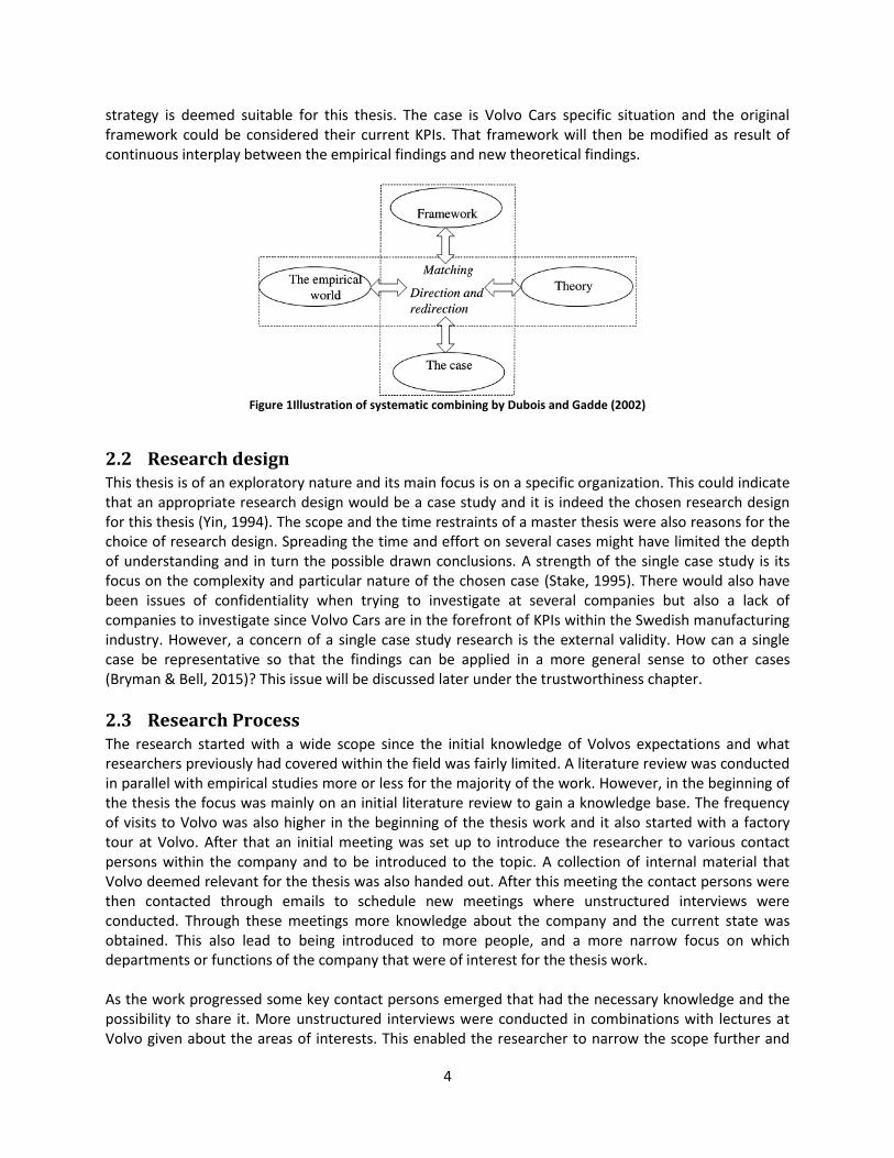
2.1 Research Strategy Bryman and Bell defines research strategy as a general orientation to the conduct of research. They identify two main clusters that are quantitative and qualitative research (Bryman & Bell, 2015). These two clusters are fundamentally different in terms of a few areas mentioned by Bryman & Bell and discussed below. Quantitative research is a research strategy that revolves around numbers and quantification in the collection and analysis of data (Bryman & Bell, 2015).The role of theory in relation to the research is a testing one, which is called a deductive approach. This means that based on existing theory, a hypothesis is stated and then confirmed or rejected at the end of data collection and analysis (Bryman & Bell, 2015). Its epistemological orientation is majorly positivism, which shortly put is a position that advocates the use of natural science methods to research (Bryman & Bell, 2015). The last area that defines the two major research strategies is the ontological orientation which concerns the nature of social entities. In the realm of quantitative research the ontological position is objectivism. This position implies that social phenomena exist independent from the social actors and beyond our reach or influence (Bryman & Bell, 2015). On the other end of the spectrum there is qualitative research. This research strategy puts more emphasize on words rather than numbers in the collection and analysis of data (Bryman & Bell, 2015). The role of theory in relation to the research is that the conducted research generates new theory, which is called an inductive approach (Bryman & Bell, 2015). The epistemological orientation related to qualitative research is called interpretivism. This is the view that within the social realm the methods used in natural science aren’t applicable to the same degree. This is because every person is unique, thus resulting in multiple accounts of perceived reality (Bryman & Bell, 2015). Qualitative research’s ontological orientation is called constructionism. This position implies “that social phenomena and categories are not only produced through social interaction but that they are in constant state of revision.” (Bryman & Bell, 2015, p. 35). This thesis revolves around developing a new KPI through interviews, analysis of current measurements and ways of doing things etc. This can be seen as more exploratory research which is primarily of a qualitative nature. Once a suggestion for a new KPI is done this could later be the topic for testing through a quantitative research. However, a clear distinction between qualitative and quantitative research is not necessarily needed, nor is it the reality of research. In fact, the two can be seen as two ends of a spectrum and not two repelling opposites and can be combined in what is commonly referred to as mixed methods research (Bryman & Bell, 2015). In the end having a framework of some sort for your research can be helpful in order to guide your choice of methods. When it comes to the relationship between theory and research a third approach exists next to the deductive and inductive approach. This is called the abductive approach to research, or systematic combining (Dubois & Gadde, 2002). This approach is more towards the inductive side but instead of theory generation it focuses on theory development. This happens as a result of a continuous interplay between empirical findings and new theoretical insights. Dubois & Gadde illustrates this approach with the figure below. This research

4

strategy is deemed suitable for this thesis. The case is Volvo Cars specific situation and the original framework could be considered their current KPIs. That framework will then be modified as result of continuous interplay between the empirical findings and new theoretical findings.

Figure 1Illustration of systematic combining by Dubois and Gadde (2002)

2.2 Research design This thesis is of an exploratory nature and its main focus is on a specific organization. This could indicate that an appropriate research design would be a case study and it is indeed the chosen research design for this thesis (Yin, 1994). The scope and the time restraints of a master thesis were also reasons for the choice of research design. Spreading the time and effort on several cases might have limited the depth of understanding and in turn the possible drawn conclusions. A strength of the single case study is its focus on the complexity and particular nature of the chosen case (Stake, 1995). There would also have been issues of confidentiality when trying to investigate at several companies but also a lack of companies to investigate since Volvo Cars are in the forefront of KPIs within the Swedish manufacturing industry. However, a concern of a single case study research is the external validity. How can a single case be representative so that the findings can be applied in a more general sense to other cases (Bryman & Bell, 2015)? This issue will be discussed later under the trustworthiness chapter.

2.3 Research Process The research started with a wide scope since the initial knowledge of Volvos expectations and what researchers previously had covered within the field was fairly limited. A literature review was conducted in parallel with empirical studies more or less for the majority of the work. However, in the beginning of the thesis the focus was mainly on an initial literature review to gain a knowledge base. The frequency of visits to Volvo was also higher in the beginning of the thesis work and it also started with a factory tour at Volvo. After that an initial meeting was set up to introduce the researcher to various contact persons within the company and to be introduced to the topic. A collection of internal material that Volvo deemed relevant for the thesis was also handed out. After this meeting the contact persons were then contacted through emails to schedule new meetings where unstructured interviews were conducted. Through these meetings more knowledge about the company and the current state was obtained. This also lead to being introduced to more people, and a more narrow focus on which departments or functions of the company that were of interest for the thesis work. As the work progressed some key contact persons emerged that had the necessary knowledge and the possibility to share it. More unstructured interviews were conducted in combinations with lectures at Volvo given about the areas of interests. This enabled the researcher to narrow the scope further and

5

create an initial version of the measure. When these things were established more specific data from Volvo could be collected for testing of the measure that was being developed. From this point the empirical study and the theoretical study continued its interplay throughout the thesis work, and where problems or difficulties arose meetings at Volvo were scheduled to help with further data collection or second opinions.

2.4 Data collection In this chapter the different methods for data collection are described.

2.4.1 Literature study

The thesis work began with an initial literature review and then proceeded as an iterative literature study throughout the project. The iterative nature derived from the unveiling of new findings and conclusions which needed literature to support those claims. The initial literature review represents an important element in all research according to Bryman & Bell (2015). The reason to start with this is to access what is already known about the topic, what concepts and theories that have been applied to the topic, who those researchers are and if there are any controversies regarding the topic (Bryman & Bell, 2015). Some topics have a vast amount of research conducted. In those situations it’s unlikely that an exhaustive literature review can be conducted considering the scope of a master thesis. What is crucial is that the key articles and books within the field are being studied (Bryman & Bell, 2015). This has been the ambition with the initial literature review. The search for literature was done through search engines such as Google Scholar and the Chalmers library database. Literature was also recommended and provided by the author’s supervisor at Chalmers. 2.4.2 Interviews

The interviews conducted for this master thesis was of a semi-structured nature. In a semi-structured interview the researcher have a list of questions related to the topic of interest. The order is however not that important and the interviewee is allowed to expand their answers and wander from the stated topic. This can lead to further questions from the interviewer that wasn’t included from the outset (Bryman, 2012). This method is one of the most commonly employed methods within qualitative research. It’s quite time consuming but it makes up for it in terms of flexibility and the ability to access in depth knowledge (Bryman, 2012). Despite these benefits the interviewer must be aware of potential pitfalls of the method. A potential source of bias is how the interviewer can influence the interviewee to answer the questions asked in a certain way. This can happen through the interviewers’ way of structuring the questions and their previous knowledge on the topic. The interviewee can also be disingenuous and provide the answers that he or she believes that the interviewer is after, or to benefit their own agenda (Bryman, 2012). The interviews that were conducted for this thesis were exploratory in nature and aimed at getting an understanding of Volvos current way of working and the individual's opinion about an OWE-measure. Interviews have been held with three production engineers involved in line balancing and process development among other things, one maintenance engineer or equipment performance responsible who were managing an improvement team consisting of other maintenance engineers and technicians. Finally interviews were also held with one productivity engineer and one technology manager that were also responsible for standards/requirements and benchmarking. The number of follow up interviews

6

varies, but it ranges from zero to three. Four interviews were held with an individual who was familiar with the line balancing of the chosen module. Some of the interviews were done casually with just taking notes about the important answers but the longer interviews that went on for 30 minutes up to two hours were recorded. This was done with the interviewees’ approval. The recording of interviews enables the researcher to fully focus on the questions and follow-up questions instead of having to take notes. It also increases the validity since it’s a way to ensure and prove that what was being said really was said (Bryman, 2012). All of the recorded interviews were revisited and the most content rich interviews were also transcribed. 2.4.3 Internal documents

Various internal documents were used by the researcher including general information about Volvo Cars Engine Skövde. Previous attempts at developing a basic OWE-measure by Volvo was handed out to gain some inspiration from. Volvos Loss model was also handed out among a few other company documents. Data on current KPI’s at Volvo was also collected in an initial stage. When the theoretical shape of the OWE-measure had been developed production data was collected from various databases at Volvo to allow for testing of the constructed excel-model. The nature of this data is described more in detail in chapter 4.4.

2.5 Trustworthiness Trustworthiness is a quality criteria proposed by Guba & Lincoln (1994) that would be more suitable for qualitative research. They felt uncomfortable with the application of reliability and validity in qualitative research since they felt that criteria presuppose that a single absolute account of social reality is feasible (Bryman, 2012). This has been deemed a suitable quality criteria since the methods employed and the nature of this thesis work have mostly been of a qualitative nature. Trustworthiness is made up of four different criteria; these in turn have an equivalent criterion in quantitative research (Bryman & Bell, 2015). These will be discussed below and how they’ve been applied to this thesis. The first criterion is credibility, which parallels internal validity. This criterion revolves around ensuring that the research was conducted using good practice and that the subjects being studied or interviewed can confirm that the investigator has correctly understood the setting and not misinterpreted the information that they provided (Bryman & Bell, 2015). To achieve credibility for this thesis triangulation was used. This means that more than one method or source of data was used, interviews, internal documents, a literature study etc. Triangulation is a way to help ensure that good practice is being used to conduct the research. The recording and the transcribing of the interviews is also a way of achieving credibility. This helps with assuring that the researcher doesn’t forget what was being said, or draws any faulty conclusions for lack of memory or notes. Another technique to ensure credibility employed by the researcher is respondent validation. This is a process where the researcher provides the people whom he or she has conducted research with, e.g. the interviewee, an account of his or her findings. The goal is to confirm that the researcher’s findings and impressions are congruent with the views of those interviewed or active at the location where the research is being conducted (Bryman & Bell, 2015). This was done by emailing interviewee’s and asking them to either confirm information or if the researcher had understood the situation correctly. Progress of the proposed OWE-measure was also presented to allow opinions on the direction it was taken and additional input. The second criterion is transferability, which parallels external validity. This concerns if the results of the study can be applied to other contexts, in other words if the results are generalizable. This can be difficult to achieve for quantitative studies and especially in this thesis since it’s only studying the single

7

case (Bryman & Bell, 2015). Instead to achieve transferability it’s encouraged by researchers to produce thick descriptions (Guba & Lincoln, 1994). Thick descriptions are basically not just providing the results, but the context of which those results apply in. This can help with explaining the choices made for the specific situation and provide a database for making judgments about the possibility to transfer the results to another context (Guba & Lincoln, 1994). This has been the ambition with this thesis. That the provided detail and context is enough for an informed person to make a decision about what parts could potentially be transferred to e.g. another company’s assembly line. However, it would have been beneficial to study multiple cases, but that has been deemed impossible due to time constraints. The third criterion is dependability, which parallels reliability. This aims to assure that the researcher hasn’t been careless or made mistakes when it comes to data-collection, the interpretation of the findings and the reporting of results etc. To help with this it’s suggested to adopt an “auditing approach”. This approach requires that the researcher keeps records of all phases of the research process. This would then enable an auditor to assess if the proper procedures have been taken (Bryman & Bell, 2015). In this research this method chapter is one of the steps taken to assure that the thesis provides the necessary information for a potential auditor (or reader) to make an informed decision about the quality and thought behind the researcher's different choices. This includes who was interviewed and how, delimitations, what literature that has been reviewed etc. The level of detail provided could have been higher but it’s still deemed sufficient for a thesis of this nature. The supervisor at Chalmers has also served as a bit of an auditor to judge the taken procedures and guide the research process. The fourth and last criterion is confirmability, which parallels objectivity. The researcher should not allow their personal values or theoretical inclinations to influence the research and in turn the findings and drawn conclusions. At the same time it’s important to recognize that complete objectivity is impossible to achieve in qualitative research (Bryman & Bell, 2015). The thesis has mainly been influenced by the supervisor and the case company’s opinions, but also of the theoretical framework that has been studied. The fact that research has been conducted by a single researcher can also potentially increase the bias of the work. It has however always been the intention of the researcher to act in good faith and to be as objective as possible. This discussion and the awareness of the issue have served as a way to try and lower that bias.

2.6 Ethical considerations When it comes to ethical considerations within research they are often revolving around four different issue areas. Is there any harm to participants? Is there any lack of informed consent? Is there an invasion of privacy? Is there deception involved (Diener & Crandall, 1978)? The issue areas have been considered when conducting the interviews. Before any of the interviews took place an email about the content and topic of the questions were sent. They were also asked for permission to be recorded and what would happen to that material afterwards. In general the researcher strived to achieve and maintain an open and honest approach when conducting the research. This applies to the people involved in the thesis and the references used, not to present anything in a dishonest way. A formal contract was also signed with Volvo Cars regarding general terms and conditions on studies carried out by students.

8

3 Theoretical framework This chapter provides the theoretical framework that has been studied and deemed relevant for the

researcher’s own work and as a background for reading the thesis. It begins with Losses in business or

manufacturing processes. This chapter brings up some of the different losses experienced in business or

manufacturing processes. This is followed by Performance Measurement System which describes the

combination of performance measures that, among other things, can measure the previously described

losses. The next chapter is called Enterprise Resource Planning and Manufacturing Execution System.

These are two types of IT-systems that can be used to collect the input data needed for the company’s

performance measures. This is followed by Time Data Management which describes the processes of

time data management which revolves around how a company collects and manages time data of e.g.

their production processes. After this comes Predetermined Time Standards which is a method for

determining time data. This is followed by Manufacturing start-up of a new process, which addresses

the difficulties experienced in this stage of a process. All of the chapters described so far aim at

providing the context in which performance measures are used and some of the enablers for effectively

using them. The remaining chapters cover already established performance measures and models. The

first in that order is called Productivity. This chapter brings up the definition of productivity,

effectiveness and efficiency and how they relate to each other. Next in line is The Kurosawa Structural

Approach, which brings up a model developed by Kurosawa to measure the overall efficiency of labor.

After this comes Overall Equipment Effectiveness which describes the performance measure with the

same name that is used for measuring losses in machines/equipment. The two following chapters are

called Overall Labor Effectiveness and Manual Assembly Efficiency and they describe two previous

attempts on performance measures related to worker efficiency. The final chapter is called Expanded

Productivity Improvement Model and it brings up a model where productivity is described as a function

of the method used, the performance and the utilization.

3.1 Losses in business or manufacturing processes

The idea of losses, or rather inefficiencies, has probably been around for as long as there has been human development. However, in more recent years Frederick Taylor developed a theory called Scientific Management. This work is commonly viewed as one of the earliest attempts to apply science to processes and management within a company-setting. Taylor starts his book with quoting then president of the United States of America, Theodore Roosevelt. The quote brings up the importance of conserving natural resources and its importance for national efficiency. While Taylor agreed with this quote he himself stated that: “But our larger wastes of human effort, which go on every day through such of our acts as are blundering, ill-directed, or inefficient, and which Mr. Roosevelt refers to as a lack of “national efficiency,” are less visible, less tangible, and are but vaguely appreciated.” (Taylor, 1911, p.5). The inefficiencies of workers are not visible in the same way as inefficiencies related to the use of e.g. materials, even though daily losses from worker inefficiencies are greater than that of material things according to Taylor (Taylor, 1911). Taylor’s work paved the way for future research regarding the identification and elimination of inefficiencies related to the workers. In even more recent times Toyota got inspired by Taylor’s Scientific Management in their development of the Toyota Production System (TPS), also referred to as Lean Manufacturing. While the system comprises of both management philosophies and practices it could be said that the foundation of the

9

“Toyota Way” is based upon the goal of identifying and eliminating waste in all work activities (Liker & Meier, 2006). Identifying the waste is however not the same as eliminating the waste and this is where TPS is describing a systematic method and way of working to achieve this goal. Nevertheless, focusing on the identified losses, or non-value-adding activities, Liker & Meier describes eight different losses in business or manufacturing processes (Liker & Meier, 2006). These losses are presented below: Overproduction: Overproduction is producing items earlier or in greater quantities than what is required by the customer. Producing more items than what is needed is a waste in the sense that it’s items that won’t get sold since there is no demand for them. Producing the items earlier than what is required by the customer generates different wastes such as overstaffing, cost of inventory etc. Waiting (time on hand): This loss is related to idle workers. The workers can be idle because they are surveiling an automated machine, or having to wait for the next processing step, tool, part etc. In an assembly line there are often balance losses of some sort that generates these types of waiting times. The worker can also be idle because of processing delays, equipment downtime or similar reasons. Transportation or conveyance: Transportation is a non-value-adding activity. Even though it is necessary, it should be limited as much as possible. This can be the moving of work in process (WIP) between different process steps but it is also the movement of materials, parts, equipment etc. in and out of storage or between different processes. Overprocessing or incorrect processing: Overprocessing is performing steps that aren’t necessary to process a certain part. These unnecessary steps can also be steps that results in a higher quality product than what was requested by the customer, which is also a waste. This loss also comprise of inefficiently processing due to poor product design and tools, which in turn can cause unnecessary motions, defects and potential rework. Excess inventory: Excess inventory can be WIP, finished goods or excess raw material. Having an excess inventory can in turn cause longer lead times, increase the risk of obsolescence and naturally an increased storage cost. Another important issue is that excessive inventory can hide long setup times, machine downtime, late deliveries from suppliers and the balance losses of the production system etc. Unnecessary movement: An unnecessary movement is any movement that the worker has to perform that isn’t value adding. Examples of this are walking in between process steps, searching for tools, reaching for something etc. Defects: The losses related to defects are the scrapping of parts, the replacement production that might have to be done or the rework to adjust the defect. Also inspection to detect defects generates waste in terms of handling, time and effort.

10

Unused employee creativity: By not listening to or engaging your employees an organization can lose ideas of improvement, skills and other learning opportunities. These losses are all related to each other in several ways, as one of them might cause the others. Taiichi Ohno who originally developed this loss model at Toyota considered overproduction to be the fundamental waste, since it is the main cause for all other losses (Liker & Meier, 2006). The losses that are related to manual labor, which this thesis is concerned with, are Waiting, Unnecessary movements, Defects, Unused employee creativity, Overproduction and Overprocessing. An employee can however not directly influence Waiting and Unnecessary movements since they are determined by how the business or manufacturing processes are designed. Overproduction and Overprocessing is also related to manual labor in a more indirect way. Overproduction leads to overstaffing, which is unnecessary man hours spent. Overprocessing leads to unnecessary process steps executed by the employees but the steps are determined, as for unnecessary movements, by how the business or manufacturing processes are designed. The defects can however be caused by an employee who’s not careful or alert, even though the methods and standard practices should strive to eliminate the possibility of making mistakes (Monden, 2011). Ohno also stated that the seven first losses directly impact the unused employee creativity. All the different wastes hide problems that would otherwise surface and force the employees to think and use their creativity to solve the underlying problems (Liker & Meier, 2006).

3.2 Performance Measurement System

In order to say something about e.g. the performance of a process, the performance must somehow be measured and compared to either similar processes, or the historical data of that process to spot the trend. Is the performance of the process improving or getting worse over time? How is the performance related to competitors? What gets measured gets managed. This is the main rationale behind the use of performance measures. Neely et al. (1995) defines performance measurement as the process of quantifying action, where measurement is the process of quantification and action leads to performance (Neely et al., 1995). Performance measures can be categorized in different groups, even though there are some different opinions regarding the definitions (Parmenter, 2010). A common distinction is however made between performance indicators (PI) and key performance indicators (KPI). The PIs help align the operations to the strategy of an organization. They are also used for managing the daily operation to meet customer demands and other requirements (Landström et al., 2016). The KPIs however, represents the set of measures that focuses on the aspects of organizational performance that are the most critical for success (Parmenter, 2010; ISO, 2014). When an organization combines a set of various PIs and KPIs it results in that organization performance measurement system (PMS) (Neely et al., 1995). Neely et al. (1995) argues that the performance measures needs to be positioned in a strategic context, as they will influence what people do. Performance measure can be categorized in many different ways and it’s up to the organization to choose what performance measures to combine and to use in order to encourage actions that realizes the underlying strategy (Neely et al., 1995). In the Swedish manufacturing industry the adoption of PMS is close to 100%, at least among medium to large companies (Landström et al., 2016). Its widespread use is closely connected to the popularity of lean manufacturing and a set of PIs can be chosen to identify and manage the losses that were presented in the previous chapter (Åhlström & Karlsson, 1996). There are different frameworks for how a PMS should be structured. The best known one and the norm within the industry is arguably the balanced scorecard (BSC) developed by Kaplan and Norton in 1992. The

11

basic idea is that BSC allows managers to look at the business from four important perspectives by answering four questions (Kaplan & Norton, 1992):

The customer perspective: How do customers see us? The internal business perspective: What must we excel at? The innovation and learning perspective: Can we continue to improve and create value? The financial perspective: How do we look to shareholders?

Related to all these perspectives are set goals with corresponding measures, as illustrated in figure 2 below. The BSC limits information overload and forces managers to focus on the handful of measures that are the most critical (Kaplan & Norton, 1992). Neely et al. (1995) however states that while it is a useful framework, there is little underlying it in terms of the process of performance measurement system design. The original BSC also contains a serious flaw since it excludes the competitor perspective with the corresponding question - what are our competitors doing (Neely et al., 1995)? This original framework has later been modified as companies have made their own interpretations and changes (Landström et al., 2016). The original BSC perspectives can be replaced with more company specific headlines for the grouping of PIs in the PMSs in order to fit that company's specific strategy (Landström et al., 2016).

Figure 2 The original structure for BSC proposed by Kaplan & Norton (1992)

On a more general note the lifecycle of a PMS can be said to have four phases: design, implementation, management and evolution (Landström et al., 2016; Bourne et al., 2000). The design phase deals with the design of the PMS (Landström et al., 2016). This means developing measures that focuses on the key objectives. Bourne et al. (2000) states that there is a strong consensus among researchers that the measures should be derived from strategy. When the PMS has been designed the next phase is the implementation. This phase is concerned with which systems and procedures to install in order to collect and process the data that enables the measurements to be made at the designed frequency

12

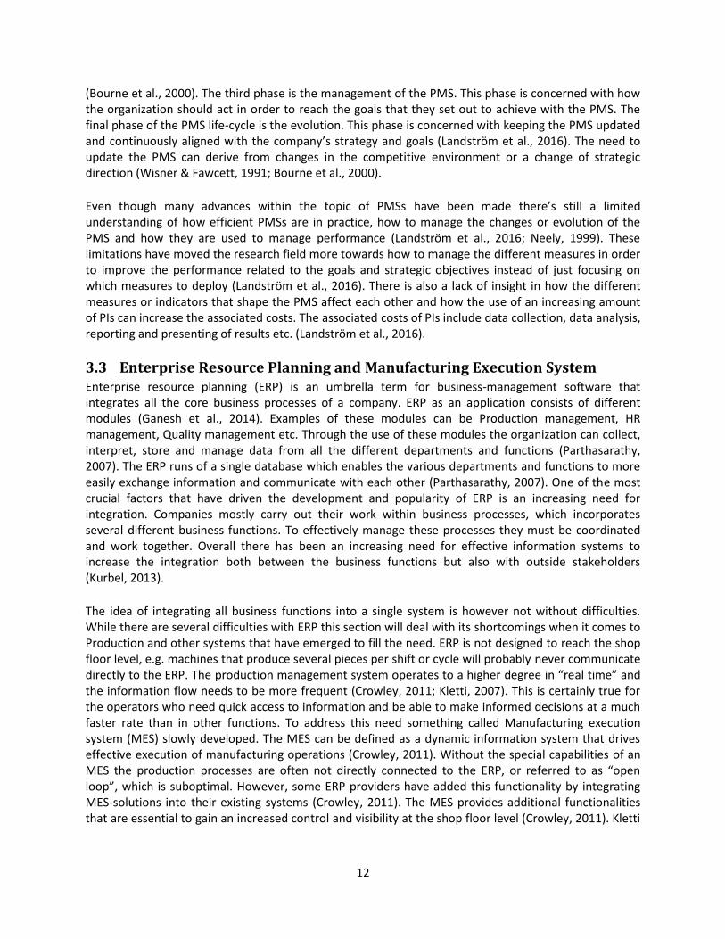
(Bourne et al., 2000). The third phase is the management of the PMS. This phase is concerned with how the organization should act in order to reach the goals that they set out to achieve with the PMS. The final phase of the PMS life-cycle is the evolution. This phase is concerned with keeping the PMS updated and continuously aligned with the company’s strategy and goals (Landström et al., 2016). The need to update the PMS can derive from changes in the competitive environment or a change of strategic direction (Wisner & Fawcett, 1991; Bourne et al., 2000). Even though many advances within the topic of PMSs have been made there’s still a limited understanding of how efficient PMSs are in practice, how to manage the changes or evolution of the PMS and how they are used to manage performance (Landström et al., 2016; Neely, 1999). These limitations have moved the research field more towards how to manage the different measures in order to improve the performance related to the goals and strategic objectives instead of just focusing on which measures to deploy (Landström et al., 2016). There is also a lack of insight in how the different measures or indicators that shape the PMS affect each other and how the use of an increasing amount of PIs can increase the associated costs. The associated costs of PIs include data collection, data analysis, reporting and presenting of results etc. (Landström et al., 2016).

3.3 Enterprise Resource Planning and Manufacturing Execution System

Enterprise resource planning (ERP) is an umbrella term for business-management software that integrates all the core business processes of a company. ERP as an application consists of different modules (Ganesh et al., 2014). Examples of these modules can be Production management, HR management, Quality management etc. Through the use of these modules the organization can collect, interpret, store and manage data from all the different departments and functions (Parthasarathy, 2007). The ERP runs of a single database which enables the various departments and functions to more easily exchange information and communicate with each other (Parthasarathy, 2007). One of the most crucial factors that have driven the development and popularity of ERP is an increasing need for integration. Companies mostly carry out their work within business processes, which incorporates several different business functions. To effectively manage these processes they must be coordinated and work together. Overall there has been an increasing need for effective information systems to increase the integration both between the business functions but also with outside stakeholders (Kurbel, 2013). The idea of integrating all business functions into a single system is however not without difficulties. While there are several difficulties with ERP this section will deal with its shortcomings when it comes to Production and other systems that have emerged to fill the need. ERP is not designed to reach the shop floor level, e.g. machines that produce several pieces per shift or cycle will probably never communicate directly to the ERP. The production management system operates to a higher degree in “real time” and the information flow needs to be more frequent (Crowley, 2011; Kletti, 2007). This is certainly true for the operators who need quick access to information and be able to make informed decisions at a much faster rate than in other functions. To address this need something called Manufacturing execution system (MES) slowly developed. The MES can be defined as a dynamic information system that drives effective execution of manufacturing operations (Crowley, 2011). Without the special capabilities of an MES the production processes are often not directly connected to the ERP, or referred to as “open loop”, which is suboptimal. However, some ERP providers have added this functionality by integrating MES-solutions into their existing systems (Crowley, 2011). The MES provides additional functionalities that are essential to gain an increased control and visibility at the shop floor level (Crowley, 2011). Kletti

13

(2007) describes the ideal MES and the functionalities it should possess which can be divided into the following areas:

The functionalities of an MES itself Communication with corporate management applications Communication with the manufacturing environment

The functionalities of an MES can be divided into three function groups according to Kletti (2007): Production, quality and human resources. These functions groups all have their related modules such as: production data acquisition, machine data collection, statistical process control, non-conformance management, short-term manpower planning etc. Crowley (2011) describes the functionality of a MES under the following headings: Materials management: Inventory and warehouse management. Includes the tracking of materials in the factory, use of barcodes and RFID data collection. Pre-production control: Includes kitting, setup verification, supply of materials and work in process-tracking. Production control: Scheduling of production, optimization of run order, assembly modeling, monitoring of the production line, tracking of the finished goods, downtime and setup times, issues of materials, manual assembly processes and electronic setup instructions. Process traceability: Enforcement of the process definitions, control and traceability of the process steps throughout the whole production facility. Quality management: Includes data collection of quality levels and defects, both for manual and automated processes. Also includes support for rework and repairs. Visibility: Access to real-time information regarding the production process as well as historical data. These functionalities of the MES must then be able to communicate with corporate management applications. That means that there must be interfaces that can communicate with common ERP systems (Kletti, 2007). The ERP system is mostly concerned with corporate management and process data in terms of quantity planning and order releases. The MES is more focused on production management and receives the order loading with corresponding dates from corporate management. Production management then carries out the sequencing and loading planning and resource management etc. In the same way as the MES communicates with corporate management, the MES must also communicate with the manufacturing environment as previously stated (Kletti, 2007). This is referred to as the production level or the automation level. That’s where the actual manufacturing of goods takes place. The MES is directly connected to the machines to acquire data and transmit machine settings etc. (Kletti, 2007).

14

Figure 3 the three levels of manufacturing companies and their data collection systems by Kletti (2007)

Figure 3 illustrates how the MES overlaps and connects to the ERP system and the automation level. APS stands for Advanced Planning and Scheduling and is bridging the ERP with the MES. At the overlap between MES and Automation there is the function of system control. This functionality permits direct data tapping within production by the MES. Figure 3 also showcases how the time horizons changes when moving from corporate management down to production management and the automation level (Kletti, 2007).

3.4 Time Data Management

This chapter is concerned with time data management (TDM). TDM doesn’t have any consistent definition within the scientific literature. It is however described as all activities that manage the factor time (Hinrichsen, 2009, Kuhlang et al., 2014). It is also referred to as an organizational unit within a company (Kuhlang et al., 2014). Within manufacturing companies TDM plays a vital role for management to be able to plan their operations and make strategic decisions. This includes production systems analysis, modeling, simulation and design of human work tasks (Kuhlang et al., 2014). Even though the necessity of TDM is clear many companies refrain from dedicating TDM to a specific function within the company. This is because they view TDM as time consuming and costly. These companies might solve the TDM related issues differently but they increase the risk of outdated time databases and lack of time-related competences by not using scientific approaches (Kuhlang et al., 2014). In recent years companies and research institutes have once again realized the significance of time as a planning, control and decision making factor (Kuhlang et al., 2014). In modern industrial engineering time data represents a work process and how the structure of the work process determines the time it takes to complete. Kuhlang et al. (2014) quote the German MTM-Association and their slogan: “the method determines the time!” concluding that not only the factor of time is important in TDM. TDM also consists of the time-relevant data such as the work methods and the rate of repetition etc. (Kuhlang et

15

al., 2014). In order to get a comprehensive view on TDM Kuhlang et al. (2014) defines it as the processes determination, pre-processing, application and administration of time data.

Figure 4 Processes of TDM by Kuhlang et al. (2014)

There are several interdependencies and overlaps between the different processes and that’s why a holistic view is important. The different process steps from the figure will shortly be described to give an overview of the TDM process. General aspects: In the figure the general aspects are grouped under determination, pre-processing and application to indicate in what step of the TDM process these general aspects are to be considered. The general aspects include what type of production the company is involved with, which serves as an indicator of suitable methods of time determination. Who manages TDM within the company/organization and is the function centralized or decentralized? An evaluation of the competencies within the company regarding TDM must also be done. If the knowledge is insufficient external support might be needed. If the time data is used to evaluate performance and remuneration is involved, worker unions might have to be involved for agreements to be signed. The final general aspects to consider are what type of time units to use (hours, minutes, seconds etc.), if the collected data can be applied in other areas (the transferability of time data) and how often the time data should be revised (Kuhlang et al., 2014). Determination: The first step of the TDM process is determination. The starting point is deciding for what areas in the company that time data should be determined (e.g. production, assembly, and logistics). Should the time data be determined before or after the start of production? Depending on the choice different methods for determining time data might be suitable. The duration of the work content, and if it is performed by a man or a machine also serves as an indicator of the time determination method. Then the actual choice of the methods to determine time must be made. Some available methods are: time studies (e.g. an observer using a stopwatch to measure “actual time”), automatic data collection by

16

machines to collect “actual time” and predetermined time studies (PTS will be explored in the next chapter) such as Methods-Time Measurement (MTM) that can be used to acquire the “target times” (Groover, 2007). The different methods also differ in work content and effort, which translates into expenditures which also must be taken into consideration when determining the methods to apply (Kuhlang et al., 2014). Pre-processing: The determined time values are normally not directly applicable for decision making. That is why the time data needs to be pre-processed. This includes distinguishing between different characteristics of time data. The determination process dealt with “actual time” and “target time”. Pre-processing also deals with standard times and standard data through statistical evaluations. The standard times contain target times and additions for rest and allowance time. The pre-processing also categories the collected time data in terms of “process building blocks”. This is done by describing the work content in a process. As more work content gets added the process gets more specific and their re-usability declines. The process building blocks gets labeled “product-neutral” which corresponds to e.g. a basic operation, “product-related” and “application-related”. An analysis of the factors that might influence the duration of work content is also necessary to conduct, as well as an analysis of the amount of value adding time of the total duration of work. This analysis serves to assess improvement or optimization possibilities. Finally the pre-processing is also concerned with presenting the time data in a proper way to ensure that it’s understandable and clear (e.g. tables, graphical representations, not too many influencing factors) (Kuhlang et al., 2014). Application: The process of application of time data distinguishes between strategic, tactical and operational characteristics and sorts the data accordingly. It also specifies the purpose of the application of time data. It can be time data of order monitoring which represents important information for operational decisions or identifying and performing time-related continuous improvement process in production systems. These data are used for internal purposes, but time data can be applied for external use as well in the context of e.g. supply chains. The different application purposes have different requirements on the accuracy of the provided time data, which is defined as the maximal accepted deviation from predefined time values (Kuhlang et al., 2014). Administration: The administration part of the TDM process deals with how the data is being stored. Centralized data storage of time data is preferable to provide a consistent time database. There also needs to be an administration system, which is related to data storage. Common solutions are various types of IT-systems. An important aspect here is the level of integration of the solution. A fully integrated system means that the determination, pre-processing, application and administration of time data occur within the same IT-system. Otherwise data exchange happens between different IT-systems (Kuhlang et al., 2014).

3.5 Predetermined Time Standards

Predetermined time standards (PTS) are advanced techniques which aim at defining the time needed to perform different operations. This is done by using pre-set standard times for the various motions (both the nature of the motion and the conditions under which it is made) to build up the time for a job at a defined level of performance and not by using direct observation and measurement (Kanawaty, 1992). Kanawaty illustrates the nature of a PTS system by looking at the simple work cycle of putting a washer

17

on a bolt. The operator will reach to the washer, grasp the washer, move the washer to the bolt, position it on the bolt and release it. These are basic motions that are part of many operations. Add to this other body motions and a few other elements and you have the components of a basic PTS (Kanawaty, 1992). One of the advantages of using PTS systems are that they lead to more consistency in setting standard times compared to stopwatch time studies. The main advantage of using a PTS system is however the fact that the standard time for an operation can be defined even before production begins. This means that it can be used in a design stage to optimize the layout and design of the workplace to achieve the optimum production time. They can also be used to make an estimation of the cost of production before starting the operation, which also is valuable for budgeting and planning (Kanawaty, 1992).

Several PTS have been developed over the years but one of the most used and arguably most important systems is Methods-Time Measurement (MTM) which was developed by H.B. Maynard, G. J. Stegemerten and J. L. Schwab and released in 1948 (Hasselqvist et. al., 1969; Kanawaty, 1992). For the first time, the full details of a PTS system were made accessible to everyone. Succeeding this, MTM also put up several non-profit-making MTM associations around the world to control the standards of training, practice and to continue the research and development of MTM (Kanawaty, 1992). At Volvo cars they’re using a PTS system that is called Sequence based Activity and Method analysis (SAM). It’s based around the first version of MTM called MTM-1 but simplified to make the analysis more quick and easy (MTM-föreningen i Norden, 2016). Volvo was a part of its development in 1982 and SAM is currently the most used PTS system in the Nordic countries (MTM-föreningen i Norden, 2016).

3.6 Manufacturing start-up of a new process

The ramp-up phase occurs when a new product is introduced, but it could also be the start of a new process or factory (Bohn & Terwiesch, 2001). This phase is defined by Surbier et al. (2014) as the beginning of commercial production and ends when the production reaches maturity. The processes of this early phase clearly differ from standard production. Approved organizational structures, policies and procedures may work well in standard production, but in these ramp-up scenarios they can be too inefficient and ineffective when it comes to generating the necessary information for correct decision making (Almgren, 2000). In the ramp-up phase the number and frequency of disturbances can overload the organization and thus affect the performance. Almgren (2000) claims that these disturbances, or the overload of them, results from the inability of a production system either to:

Identify the conditions that cause disturbances, or Take actions to correct conditions that are likely to lead to disturbances once such conditions

are identified (disturbance prevention). He then lists the four main sources of disturbances:

Materials supply (lack of materials and the quality of it) Production technology (potential breakdowns, stoppages etc.) Personnel (individual learning, the work performance) Product concept (engineering changes)

All of these disturbances affect the quantity performance negative and overtime was used to make up for the losses in the specific case that Almgren was studying (that of Volvo S80). For the quality performance, mainly materials supply and product concept affected the outcome (Almgren, 2000). All of these disturbances resulted in an increased cost of manufacturing as measured by the number of man hours compared to a standard cost target. In conclusion the focus in a ramp-up phase should be to

18

identify the disturbances. This can be done through adopting certain principles for designing, planning and controlling (Almgren, 2000). The control aspect is more related to the topic of this master thesis, with a focus on KPIs. In Surbier et als. (2014) literature review they mention some researchers view on how to deal with the monitoring of disturbances using KPIs. Juerging and Milling (2006) states that: “the objective during the manufacturing start-up is to attain quality and quantity targets with a predetermined production lead time at the lowest possible cost”. This is in line with what Almgren was stating earlier. He endorses the use of a capacity performance index (the ratio between number of produced cars, and the number of planned cars), a quality performance index (number of non-faulty cars and number of produced cars) and a cost indicator (the extra man hours to make up for lost capacity, inspection and corrections) (Almgren, 1999). Juerging and Milling (2006) states that there are two major variables that affect the efficiency of the production process during ramp-up, more precisely productivity and quality. The quality variable is influenced by four major factors which interestingly are related to the worker: average skill of the assembly workers, work adequacy, schedule pressure and fatigue (Juerging & Milling, 2006). There are many ways of choosing indicators and these are just some examples deemed relevant for the thesis work.

3.7 Productivity

On the topic of performance measures it is often easy to get confused with the definitions and the terminology. Since this topic isn’t an exact science there can exist many variations and definitions that are specific for a certain industry or a company. One of the most important performance measures for companies is productivity (Petersson, 2000). This performance measure can be defined and measured in several ways but almost all of them are based on this general definition (Sumanth, 1984): Productivity = Output/Input. The output is defined as everything that brings value to the customer and the difference between input and output is thus regarded as the waste of the process (Rolstadsås, 1995). High productivity is reached when a company can produce what the customer wants with minimum input. The productivity can be calculated on different levels. You either compare the output related to one input source, this is called a partial productivity measure, or you can move through a spectrum of different level inputs until you have included all sources of input. Example of inputs can be labor, equipment, materials, facilities etc. (Sumanth, 1984). In manufacturing processes, the emphasis has traditionally been on labor productivity (Buzacott & mandelbaum, 1985).This performance measure is generally defined as output per hours worked, meaning that an increase in productivity requires the same level of production while reducing the size of the workforce or to produce more with the existing employees (Monden, 2011). Petersson (2000) argues that this use of the labor productivity measure may direct development efforts to solely focus on cost reductions. This might not be sufficient to maintain a competitive advantage and he brings up an article by Skinner (1995) talking about the risk of ignoring the opportunity to use manufacturing as a strategic resource and only focus on the efficiency of factory workers. Instead Petersson (2000) emphasis the necessity to give productivity a broader definition and focus. 3.7.1 The relation between productivity, effectiveness and efficiency In the literature there is no widely accepted relation between productivity, effectiveness and efficiency. However, Petersson (2000) argues that there is indeed a common overall relationship between the three terms but that the productivity function will differ for a manual assembly process in comparison with an automatic machining process. To begin with, what are common definitions of effectiveness and efficiency? Sumanth's (1984) definition of effectiveness is that it reflects how well a set of results is accomplished, while efficiency reflects how well the resources are utilized to accomplish the results. A

19

simple way of stating it is that effectiveness means doing the right things and that efficiency means doing things right (Sink & Tuttle, 1989). Now let’s return to the relationship between the three terms. In order to define productivity in a specific process, the exact definitions of effectiveness and efficiency in that process must be known (Petersson, 2000; Jackson & Petersson, 1999). Petersson strives to achieve this for a manual assembly system. The picture below shows examples of measurable losses in a manual assembly process and their relation to effectiveness and efficiency. The three time elements that are deemed important for defining effectiveness and efficiency are also stated. It’s the total work time, ideal assembly time and value-adding time. The total work time is the sum of registered time for all assemblers in the process (Petersson, 2000).

Figure 5 Examples of measurable losses in a manual assembly process and their relation to effectiveness and efficiency by

Petersson (2000)

The efficiency of a manual assembly process means to what extent the total work time is actually spent on the assembly operations. The losses that reduce efficiency are indicated by the yellow color. Rework is extra work that has to be performed after failure to meeting the specifications. Allowance time is the non-efficient time spent on various types of breaks, such as toilet breaks. Idle time is exemplified by Petersson as poor communication between assemblers. Speed losses are caused by assemblers not working at the agreed work-pace level and Etc. are added to incorporate any other potential losses (Petersson, 2000). Petersson even states that the list of losses are not intended to be comprehensive, but just function as a way to cover the most common ones and get the message across. When you subtract all these losses from the total work time you get the ideal assembly time. This time is defined as: “the shortest possible time to perform an assembly operation under good ergonomic conditions, given a certain product design and a certain assembly system.” (Petersson, 2000, p. 79). An important point here is that the efficiency is dependent on how well the existing assembly system and product

20

design are being utilized (Petersson, 2000). The efficiency for a manual assembly process can be roughly described as the following (Jackson & Petersson, 1999).

Equation 3.6.1.1

Where: = efficiency

= ideal assembly time = total work time

Moving on, the effectiveness of an assembly process reflects to what extent the ideal assembly time is used to add value to the product. The added value is the aspects of the product that the customers are prepared to pay for. This in turn translates to the losses listed in the picture where an example of time due to difficult operations could be poor access to the assembly area and other time-inefficient design choices. The walking time-loss has to do with poor assembly system layout and unnecessary movements that could be considered waste. Similar to the efficiency losses this list isn’t very comprehensive either. In general the effectiveness is mostly dependent on the product design and the assembly system design and is hard for the assembler to influence directly (Petersson, 2000). The effectiveness for a manual assembly process can be roughly described as the following (Jackson & Petersson, 1999).

Equation 3.6.1.2

Where: = effectiveness = value-adding time = ideal assembly time Now that the effectiveness and efficiency for a manual assembly process have been defined they can be related to the productivity of that process. Petersson (2000) have adopted a common view with Sink and Tuttle, and that is defining productivity as the product of effectiveness and efficiency (Petersson, 2000). On the basis of this, the productivity for a manual assembly process can be roughly described as the following (Jackson & Petersson, 1999).

Equation 3.6.1.3

Where: P = productivity

= effectiveness

21

= efficiency

= value-adding time = ideal assembly time = total work time This definition is in accordance with the basic definition of productivity stated in the beginning of this section, where output was defined as the value adding activities and then divided by the total input of the process (Rolstadås, 1995).

3.8 The Kurosawa structural approach

In Productivity Management: a practical handbook, Joseph Prokopenko (1987) brings up a model created by Kurosawa (1980) for productivity analysis. He states that a worker’s productivity (Pw) is defined as follows: Pw = output / Input of worker’s effort

Figure 6 Structure of work-hours by Prokopenko (1987)

With the structure of work-hours shown in figure () he constructs the following ratio system:

( ) ( )

Equation 3.7.1

Equation 3.7.2

Equation 3.7

22

Where:

= standard work-hours (quantity produced x standard time)

= total input work-hours (number of workers on payroll x duty hours)

= effective work-hours

= ;

= input work-hours

= work-hours omitted from this account such as work-breaks, mealtime, cleaning and maintenance time,

transport time

= lost time due to supervisor or management such as breakdown and repair, shortage or defects of materials

or parts, last-minute assignment to another task

( ) = ratio of effective work-hours to input work-hours

( ) = ratio of input work-hours to total input work-hours

=

; process efficiency

= overall efficiency of labour

= worker efficiency.

The above equation expressed in words is then the following:

Overall efficiency of labour = worker’s efficiency x ratio of effective work-hours x ratio of input work-

hours = process efficiency x ratio of input work-hours.

3.9 Overall Equipment Effectiveness: Overall equipment effectiveness (OEE) is a performance measure originally created by Seiichi Nakajima that is being used to monitor production performance, but can also serve as an indicator for process improvement activities and benchmarking (Sohal et al., 2010; Andersson & Bellgran, 2015). OEEs original definition by Nakajima comprises what he refers to as the six big losses. Through a bottom-up approach an integrated workforce should strive to eliminate these six big losses to achieve OEE (Nakajima, 1988). The losses are activities that spends resources but create no value in return (Bamber et al., 2003). Nakajima (1988) defines the six big losses as the following: Downtime losses:

Breakdown losses are defined as time losses caused by reduced productivity and quantity losses caused by defective products.

Setup and adjustment losses are the result of downtime and defects caused by changing the production configuration between different products.

Speed losses: Idling and minor stoppages losses are caused by temporary malfunctions or when a machine is

left idling. Reduced speed losses are the difference between equipment design speed and the actual

operating speed

Quality losses: Quality defects and rework are losses caused by malfunctioning production equipment.

23

Start-up losses are yield losses. They occur in the phase between machine start-up and stabilization.

OEE is measured in terms of these six losses which is a function of availability, performance rate and quality rate (Bamber et al., 2003; Dal et al., 2000). The figure below illustrates the losses and how they relate to the availability, performance rate, quality rate and how the OEE is calculated (Nakajima, 1988; Andersson & Bellgran, 2015). The figure represents Nakajima's (1988) original definition of OEE and the formulas can also be expressed as the following:

Equation 3.8.1

Equation 3.8.2

Equation 3.8.3

Figure 7 Definition and computation of OEE by Andersson & Bellgran (2015)

3.10 Overall Labor Effectiveness

Kronos Incorporated is a U.S. - based workforce management software and services company that believes that the workforce management is key in order to stay or become more competitive. They have developed an analysis tool for quantifying, diagnosing and predicting the performance of their

24

workforce. They call this measure Overall Labor Effectiveness (OLE). In short, OLE revolves around the analysis of the cumulative effect of three workforce factors have on productive output defined by Kronos as follows (Kronos, 2007): Availability: For availability the utilization is the most important component. This includes employee illness and approved or unapproved leaves, standard labor utilization measures in other words. The utilization is also affected by material delays, idle time, shift-changeover and machine downtime. Availability also includes scheduling which involves having the right skill at the right time considering your workers different competences. The calculation is basically: Availability = Time operators are working productively / Scheduled time (Kronos, 2007). Performance: The amount of products delivered and if it took as long as the labor standards indicated it would. This is affected by the availability of processes, instructions, tools and materials, training and skills of your employees and indirect support staff such as maintenance technicians etc. The calculation is as follows: Performance = Actual output of the operators / the expected output (or labor standard) (Kronos, 2007). Quality: Quality is not only affected by the material used but also by the knowledge of the employees and proper use of instructions and tools. Did they have the knowledge about the quality drivers and when to stop production for corrective actions etc.? Did the workers use the right tools and follow the instructions? These human factors are important to follow up on. The calculation for quality is: Quality = Saleable parts / Total parts produced (Kronos, 2007). These three factors incorporates a lot of the acknowledge losses in Volvos loss model but are a bit more organized under the headings and results in an OLE-value when multiplied for a cumulative result. What you in the end choose to add under each factor, or rather follow up on is up for debate, but simplifying can still yield interesting results. The fact that the OLE-measure mirrors the already established and well-used OEE-measure is an advantage. Both measures are concerned with availability, performance and quality. This resemblance can seem as a simple way of structuring things but the impact of using the same terminology can be huge in a big organization where confusion easily can arise between different departments. It’s important with a common language and platform to reach a common ground, if not you get stuck arguing over the basics and talking past each other.

3.11 Manual Assembly Efficiency

Petersson (2000) suggested an alternative measure to OEE for use in manual to semi-automatic production systems. He called this new process efficiency measure Manual Assembly Efficiency (MAE) and it’s presented below.

∑ (

)

( )

Equation 3.10.1

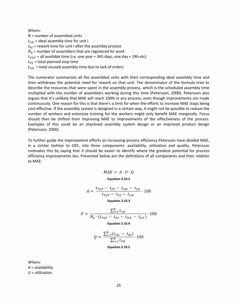
25

Where: N = number of assembled units = ideal assembly time for unit i = rework time for unit I after the assembly process = number of assemblers that are registered for work = all available time (i.e. one year = 365 days, one day = 24h etc) = total planned stop time = total unused assembly time due to lack of orders The numerator summarizes all the assembled units with their corresponding ideal assembly time and then withdraws the potential need for rework on that unit. The denominator of the formula tries to describe the resources that were spent in the assembly process, which is the scheduled assembly time multiplied with the number of assemblers working during this time (Petersson, 2000). Petersson also argues that it’s unlikely that MAE will reach 100% in any process, even though improvements are made continuously. One reason for this is that there’s a limit for when the efforts to increase MAE stops being cost-effective. If the assembly system is designed in a certain way, it might not be possible to reduce the number of workers and extensive training for the workers might only benefit MAE marginally. Focus should then be shifted from improving MAE to improvements of the effectiveness of the process. Examples of this could be an improved assembly system design or an improved product design (Petersson, 2000). To further guide the improvement efforts on increasing process efficiency Petersson have divided MAE, in a similar fashion to OEE, into three components: availability, utilization and quality. Petersson motivates this by saying that it should be easier to identify where the greatest potential for process efficiency improvements lies. Presented below are the definitions of all components and their relation to MAE:

Equation 3.10.2

Equation 3.10.3

∑

( )

Equation 3.10.4

∑ (

)

∑

Equation 3.10.5

Where: A = availability U = utilization

26

Q = quality = all available time (i.e. one year = 365 days, one day = 24h etc.) = total planned stop time = total unused assembly time due to lack of orders = total unplanned stop time N = number of assembled units = ideal assembly time for unit i = number of assemblers that are registered for work = rework time for unit I after the assembly process

Through some practical application of MAE Petersson concludes that the measure is possible to use within the industry, i.e. that the input parameters are possible to collect. The measure can give an early indication of the performance of a process. Through analysis of the input data it’s also deemed sufficient to identify losses that otherwise are difficult to spot. Examples of losses could be time-smearing and over-employment (Petersson, 2000). Next up another proposed measure for worker efficiency will be described, or effectiveness as they claim. This measure is less theoretical and developed by a management software company.

3.12 Expanded Productivity Improvement Model

Sakamoto (2010) stated that a key to successfully reaching a higher level of productivity one should separate productivity contents into method (M), performance (P) and utilization (U). This relation can be expressed in the following equation:

Equation 3.11.1

The method-factor is defined as the inverse of the ideal cycle time for the specific work-task (Almström, 2013). The largest productivity potential lies in method improvements since a specific method often has a productivity roof that can be reached achieving maximum performance or efficiency, but needs a new method to climb to even higher levels (Sakamoto, 2010). The method should constantly be revised. Volvo have clear work descriptions where they have divided the tasks that compose the station time in non-value added (NVA); necessary non-value added (NNVA) and value added (VA) time. Through constant improvements NVA and NNVA can be eliminated to increase the ratio of (VA man hours/Analyzed Direct Man hours). This is related to the “non-value-added direct work losses” from the loss model at Volvo. The performance-factor is corresponding to the speed that the work is carried out at in relation to the ideal cycle time (Almström, 2013). The performance can be above and below 100%, where 100% is the normal speed which is set through MTM. The performance rate is lower for workers that are not fully trained yet and for people with disabilities (Almström, 2013). The utilization-factor is the time spent on performing the actual work in relation to the total planned time. This factor can’t go above 100% and the total planned time is usually defined as the paid working time minus planned stops (Almström, 2013). This formula for assessing potential productivity improvements can be expanded to incorporate more detail in the analysis. The performance-factor is tied to the individual but is also affected by possible restraints or enablers of the system. The utilization-factor is also affected by the individual but even more dependent on the system and its surroundings (Almström, 2013). This has led to an expansion of the performance and utilization factors. Almström (2013) suggests dividing the performance-factor into

27

two separate, but not necessarily independent sub-factors: Personal performance (PP) and Skill based performance rate (Ps). The skill based performance rate has to do with whether the specific worker has the skill or competence required to perform the work task. For a new employee it might take some time to get fully trained. This factor is often set to a default value for these new employees, for example 50%, but it’s not actually measured. Most companies at least account for this factor since it affects the production plans and adjustments could be needed such as having an additional employee to cover up initially (Almström, 2013). The personal performance factor considers the fact that different workers have different prerequisites to perform at a higher level than the average. Reasons for this higher performance can be motivation or physical ability. This is rarely accounted for by many companies since it would require special systems put in place to examine the workers and match their salary after their performance. This could also sprout dissatisfaction and disputes among employees, managers and work unions (Almström, 2013). However, a closer examination of the employee's actual performance could help balance the overall system and raise awareness for areas/methods that might hamper performance. This could be especially valuable in the case of a system development project. However, there is an issue of defining performance and how to measure the performance differentiation among employees (Almström, 2013). For example, the time to complete the work-tasks could be measured and compared to the agreed MTM-rate. If the system could log every separate time during the day and then calculate a mean and save it, this would provide good data for decision making. It’s important to keep track of performance in the early stages since the system is not running as smooth as it could and it’s still relatively easy to make adjustments. This can help balance the system, employing the right amount of workers.

The utilization-factor can also be split into two separate sub-factors: The Need based utilization rate (UN), System design utilization rate (US) and The Disturbance affected utilization rate (UD) (Almström, 2013). The need based utilization rate is individual, but it is usually set by the system. This is the time set for short breaks and rest from fatigue and the rate is normally set to around 9-10% (Almström, 2013). This is probably already set to a fix value by an agreement between Volvo and the worker union and difficult to change. The system design utilization rate is the designed balance loss on an assembly line or the waiting time rate when operators are waiting for a machine to process (Almström, 2013). In the case of a manual assembly line, this factor is usually rather small and decreases with an increasing takt-time. For mixed model lines this factor can grow as a result of change over times. The case of machine operations is a different story. Here the factor depends largely on the level of automation in the process and how you deal with increasing the utilization of the operator in that case (Almström, 2013). The final utilization-factor is the disturbance affected utilization rate. This factor is fairly simple and it’s all the random disturbances that can occur. Disturbances such as: machine breakdowns, lack of material etc. (Almström, 2013). Volvo currently keeps track of these disturbances which is good for input in this model. All these factors make up the expanded productivity improvement model at activity level:

Equation 3.11.2

4 Present Overall Work Efficiency at Volvo: To provide some additional background Volvo’s present overall work efficiency definition will be described. This OWE-measure is presented in their “Loss-model” which is part of Volvo Cars Manufacturing System (VCMS), or more specifically in their Business Management System (BMS) under Continuous improvement. In this document they define overall work efficiency (in manual processes) as:

28

Equation 4.1

Where: Total man hours = full time employees (FTE) Value added man hours = the man hours the customer pays for These total man hours comprise of the time spent by white collars (WC) and the total time spent by the blue collars (BC). The blue collars in turn experience four types of losses. The losses for the blue collars are Excessive manning losses, Management losses, Balancing losses and Non-value added direct work losses. When these losses are removed including the time spent by white collars, you are left with the value added man hours. In order to improve this OWE-measure you have to eliminate the losses, or rather try to reduce them as part of a continuous work. The first loss “Excessive manning losses” consists of losses caused by “off standard” production, absence, restrictions and external factors. Subtracting the hours required to operate (RTO) from the total BC man hours results in the Excessive manning losses. A more detailed list of the losses under this category includes:

Volume loss & Overtime o Volume deviation loss = man hours not used due to planning fluctuation or because of

employees working overtime o Starved and blocked due to external factors o Unplanned repair, refit and adjustments o Internal Equipment Effectiveness (IEE) deviation resulting in reduced line speed

Part-time / Long-term absenteeism o People working part time or on leave of absence

Additional manning losses o Structural inefficiency, manpower not needed, workers not able to perform at the

agreed work pace level Launch related losses

o Project functions = Man hours financed by projects o Tests done due to new products or processes o Startup losses caused by uncertainty of new products/processes o Training due to launch of new products/processes

Reserve people (direct reserve) o Short term absenteeism, illness, individual holidays, training paid by government,

training law connected, local agreed leaves => ROP addition ROP = Required On Payroll = Direct and indirect hourly man hours required for production including dimensioning for volume, mix, short-term absence, individual holidays, Illness and local agreements.

The second loss category included in the model is “Management losses”. These losses are defined as man hours caused by management decisions including organizational setup. The management losses consist of production support and management losses, which seem a bit confusing. A better name for this loss category would be organizational losses, with the sub-categories production support and management losses to avoid confusion. A more detailed list of the two sub-categories is presented below:

Production support

29

o Production engineering support, Human resources, administration support and indirect process quality assurance

o Facility maintenance: maintenance on buildings and infrastructure o Process maintenance: maintenance on equipment etc.

Management losses o Man hours spent by team leaders outside balance, man hours used for team meetings,

man hours used for improvement activities (e.g. updating scorecards, doing preventive maintenance etc.) and training required to operate the existing processes with existing products, financed by production.

o Check, repair and refit outside balance (planned) o Testing: related to daily normal production verification o Paid lunch and stops (e.g. stop time end of shift) o Takt-time included relief allowances o Off-the-job training on generic and leadership competences

The third loss category is “Balancing losses”. These losses are defined as losses that occur when the work content is less than the analyzed man hours at agreed work pace level allows. They can also be defined as: Direct labor (balanced direct work) - Analyzed direct man hours = Balancing losses. The two sub-categories are presented in detail below:

Workload & Pace union agreements o Agreements on work process analyze and balancing, e.g. some workstations cannot be

running 100% work loaded for different reasons. o Overspeed → to get netto required output o MTM rate manual work

Balance loss o Shift pattern deviation: The working hours according to the shifts are not aligned with

the takt-time and required volumes o Mix loss: The different variants/models are not in an optimized sequence o Variant loss: Deviations in work content between variants causing balance loss o Model loss: Deviations in work content between models causing balance loss o Layout loss: Occurs when the layout prevents optimized balancing

The fourth and last loss category is “Non-value-added direct work losses”. This category consists of Non-value added activities (NVA) and Necessary non-value added activities (NNVA). NVA are activities that add no value to the product/service for the customer (internal and/or external). This is a common concept within lean and is usually referred to as waste (Monden, 2011). Examples of this can be unnecessary movements by workers, extra handling of material or tools and repairs/rework. NNVA are also somewhat self-explanatory activities, that is activities that are needed to make the assembly but in themselves not adding anything of value for the customer (internal and/or external). Examples of this can be cleaning of equipment, unloading parts out of machines, documentation etc. (Monden, 2011). What is then left out of the total available time or FTE (Full time employees) after subtracting all these losses are Value added man hours (VA).

30

Figure 8 Volvo cars Loss model: losses in man hours

This is a fairly straight forward way of measuring OWE. It’s the value adding man hours divided by the total man hours. The VA, NVA and NNVA activities are analyzed through MTM for every station at the assembly lines at Volvo and are clearly stated in the work descriptions that are also available at every station. However, there are some shortcomings with this way of measuring OWE. First off it can be complicated to use the “Value adding man hours”. The definition of what is VA and NNVA or NVA can be vague in some cases, making the composition of the three components vary depending on who’s making the assessment. There’s also a risk of the person responsible for the assessment being biased and more inclined to define parts of the work content as VA. The assemblers on the other hand have no way of influencing the work content to increase the amount of VA time. This doesn’t have to be a problem for an OWE-measure but one could argue that a worker efficiency measure should focus on the amount of time that the worker is actually performing the provided work content. The percentage VA time can instead be enhanced through other improvement efforts. Another issue lies in the denominator. The “Total man hours” is defined as total FTE BC + WC. The WC consists of all supporting departments, but there is no definition of which these departments are and how their time spent should be accounted for. Can all of their spent time be used in the measure, or is it only a percentage of it that should be used when calculating OWE? In general there is an ambiguity with Volvo's suggested OWE-measure. The Loss-model brings up all the experienced losses but they are just described. They are only incorporated in the measure in the sense that the pool of “Total man hours” will increase because of the experienced losses. Because of this Volvo’s OWE-measure might lack the capability to track the result of the improvement efforts carried out. For example, the loss category “Excessive manning losses” includes manpower not needed. Let’s assume that they can decrease those hours by two FTE. However, in relation to the “Total man hours” that might be a very small change, only changing the OWE-result by less than a percentage. Again, this might not be an issue but having a wide definition of the OWE-measure can make it lack the necessary focus and clarity for decision makers. This certainly true for the prioritization between different improvement efforts. If a redefinition of what should be defined as VA time have a greater impact on OWE than decreasing excessive manning its usage might be limited. Another example where the measure lacks the necessary detail is for

31

“Additional manning losses” where it brings up worker not able to perform at the agreed pace level. That doesn’t actually impact the OWE-measure since that assembler is still accounted for as a FTE. If the assemblers slower performance results in less output, that isn’t captured by the OWE-measure either.

5 The case: Outer assembly at Volvo Volvo Car Corporation is a Swedish automobile manufacturer that was established in 1927 by Assar Gabrielsson and Gustav Larson as a subsidiary company of the bearing manufacturing company SKF. Up until 1999 Volvo Car Corporation was part of the Swedish Volvo group, but was then acquired by the Ford Motor Company. Their ownership lasted until 2010 when Volvo Car Corporation got acquired by the Chinese company Zhejiang Geely Holding Group which are the current owners. Volvo Car corporation have their headquarter situated in Torslanda, Gothenburg and currently employ about 29000 employees worldwide. The production takes place in Sweden, Belgium, China and Malaysia (Volvocars.com, 2016). Volvo Cars Engine in Skövde is concerned with machining and assembly of the car engines which are later transported to car plants in Torslanda, Gothenburg and Ghent, Belgium for the final assembly into cars. The plant in Skövde currently employ 1883 employees and have a plant capacity of 530 000 engines/year. The plant structure in Skövde is Component manufacturing, Base assembly and Final assembly. In Component manufacturing engine blocks, crankshafts, camshafts and cylinder heads are produced. These parts are then being put together in Base assembly, also referred to as Inner assembly. The next step is the Final assembly, where the engines can branch of into more variants from the base assemblies. This is also referred to as Outer assembly. The engine models produced in the plant, not counting all the variants of each, are 5-cylinders diesel, 4-cylinders petrol and 4-cylinders diesel. This thesis is focused on Outer assembly, or more specifically on the “S-factory”, where the assembly of petrol and diesel engines are done. The assembly line in the S-factory is shaped like an S and consists of four different modules. The modules work in pairs, where two focus on petrol engines and two focus on diesel engines. To narrow the scope further this thesis is concerned only with the diesel modules.

Figure 9 The flow chart of Outer assembly

32

Figure 9 represents the flow-chart for a single module at Outer assembly. The black symbol represents inner assembly and this is where the engines arrive from. The engines move with an AGV-system (automated guided vehicle) so their movement is done automatically. The engines then stop at a small buffer and then enter the system. There are four sling-teams where the actual assembling is taking place; these are indicated by the yellow and blue dots. Every sling comprise of eight stations, at least schematically. In reality some stations are not operational for certain models/variants. The second sling, indicated by blue color have some stations included were the assemblers move outside of the sling. There they perform some extra tasks concerning the finishing up of the engines, like putting on plastic covers etc. These stations are included in the rotational loop for sling two. Every sling has a team leader who deals with managerial tasks but is also available approximately 50% of their time to perform assembly tasks in the line, if required. In the system there are also included two rotational spots for truck drivers taken up by the regular assembly workers. These truck drivers supply certain material for the four assembly slings but are not part of the material handling function that is also active in the system. The SIP (single inspection point) station, indicated by the red color, is situated after the assembly slings. Here a single worker is performing inspection and can trace errors back to who performed it for fast feedback and corrective measures. The final part of the system is the two test-stations where the engines are hooked up and subject to a test-sequence. This is performed by a single worker at each test-station where three engines are tested at a time. After this the finishing up tasks performed by assembly sling two is made and the engines move off to shipping or a finished goods warehouse for a brief storage.

5.1 Line-balancing and performance targets In order to set standard times for manual operations or tasks Volvo uses MTM-SAM. In the same fashion as with any MTM-system you can determine these standard times in which the average worker should be able to perform a specific task. This time is then set as a norm, a 100%-performance, where a performance below 100% is a worker taking longer time to complete the task and vice versa. These types of systems are necessary to use when production technicians try to balance the work content of e.g. an assembly line. In Volvo's assembly line they have a system takt-time of 76 seconds. This means that every 76 second the engines should move from one takt-time i to the other. It is then up to the production technicians to balance the work content of that takt-time i to equal 76 seconds. This is hard to achieve and the total work content of a takt-time i is usually a bit below the target of 76 seconds, but never above it, since that would make it a bottleneck of the system. What then is a station in this context? Some clarification is needed to avoid confusion. A station is usually defined as a single stop for the product/part being processed. In this case the AGV-carrier making a stop to allow the assembler to conduct some sort of work with machines or tools nearby. The station-time i is often the same thing as the takt-time i. This is however not always the case. Multiple stations can instead be combined to try and equal the takt-time of the system. Reasons for this can be machinery and tools that can’t fit in the same area or for some other reason that makes it practical to divide the stations. This difference between a takt-time i and a single station is important to understand and be aware of. The “station-thinking” can make the production system more static. The concept of a takt-time is more flexible for the production engineers and allows them to combine stations and rearrange groups of work tasks to equal the takt-time of the system. At Volvo cars in Gothenburg this concept is more in place, except they refer to it as a “balance” instead of a takt-time. Another topic that needs to be addressed to avoid confusion at Volvo is the idea of the performance and the performance goals for the workers. At Volvo they have a 114%-performance goal set for the workers, meaning that they should work 14% faster than the standard times set in MTM-SAM. In the

33

past this was related to a contract rate, as workers who performed at this speed were paid more. Today this salary-system is not in place anymore and all workers are paid the same salary for the amount of hours they’ve worked. The 114%-performance goal has still remained as a way of staying competitive, or by the means of tradition. So, what does this mean in reality? To exemplify let's assume that a station has the station time 74 seconds. The analyzed work content in MTM-SAM 100%-performance have then been approximated to be about 84 seconds. That is simply 84/1.14 = 74, an easy way of achieving a 114%-performance. However, often the work content is composed of both manual tasks, and machine-time where an engine is being processed or a tool is put to use. Let’s assume the work content consisted of the parts accounted for in the table below:

Station time Manual work (114%)

Machine time (100%) Manual work (114%)

74s 20s 34s 20s

The only work content that have been subjected to the 114%-performance are the two manual tasks. This is the type of calculations that are made for line balancing and the balance of work content at a station. When observing the whole line or rather the output of the system, the situation gets a bit more complicated and this is probably where the confusion happens. The planning takt-time at Volvo is set to number of engines per hour and there is a “takt-template” used in production for scheduling and planning purposes. The highest output level in the template is 35.25 engines/hour and is an estimate of the actual output to help with the planning process. Let’s calculate backwards to display where this number originates from. If the station takt-time is 76 seconds that would mean 3600/76 = 47.4 engines/hour. In a sling-team there are eight stations and seven workers. It’s decided that one station should be empty to serve as a leveling buffer. This means an output of (⅞)*47.4 = 41.5 engines/hour when working without interruptions and the current setup with seven workers. However, there are regulations for personal breaks for the employees, like going to the bathroom, allowing time for shorter meetings etc. These rates are decided and agreed upon by the unions and Volvo cars as an employer. It’s called allowance and it is currently set to 8%. For the theoretical output this means 41.5/1.08 = 38.4 engines/hour. Finally, this output is only achieved when there are no interruptions or breakdowns, which of course isn’t the case. The theoretical efficiency of the system is calculated to: η = 91.8% which accounts for all the occasions when the system isn’t producing. This leads to the final adjustment to the output: 38.4*0.918 = 35.25 engines/hour which is used for planning purposes to account for the different production losses in the system. To summarize, the 114%-performance doesn’t mean that Volvo would produce 35.25/1.14 engines/hour if they worked at a 100%-performance level. The 114%-performance is applied to manual tasks when balancing the work content to equal 76 seconds. The planning takt-time on the other hand is a way of estimating the actual output of the system and the variables affecting that is the allowance, the theoretical efficiency of the system and the quota between number of workers and stations in a sling-team. Also worth noting is a reflection about the worker's actual performance. If a station's work content is balanced to equal 72 seconds instead of 76, the worker has a 4 second marginal. What often happens is that the worker doesn’t work at a 114% performance for 72 seconds, but rather work at a lower performance to finish it in 76 seconds instead, making the actual performance level vary as a result.

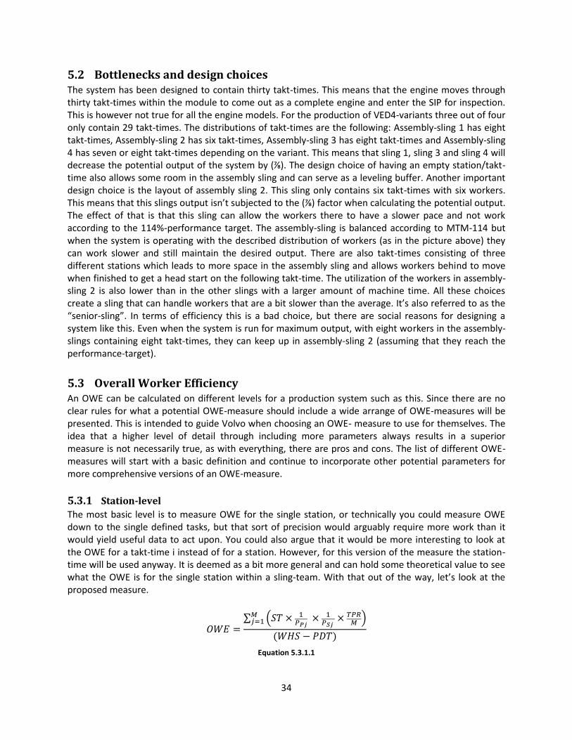
34

5.2 Bottlenecks and design choices The system has been designed to contain thirty takt-times. This means that the engine moves through thirty takt-times within the module to come out as a complete engine and enter the SIP for inspection. This is however not true for all the engine models. For the production of VED4-variants three out of four only contain 29 takt-times. The distributions of takt-times are the following: Assembly-sling 1 has eight takt-times, Assembly-sling 2 has six takt-times, Assembly-sling 3 has eight takt-times and Assembly-sling 4 has seven or eight takt-times depending on the variant. This means that sling 1, sling 3 and sling 4 will decrease the potential output of the system by (⅞). The design choice of having an empty station/takt-time also allows some room in the assembly sling and can serve as a leveling buffer. Another important design choice is the layout of assembly sling 2. This sling only contains six takt-times with six workers. This means that this slings output isn’t subjected to the (⅞) factor when calculating the potential output. The effect of that is that this sling can allow the workers there to have a slower pace and not work according to the 114%-performance target. The assembly-sling is balanced according to MTM-114 but when the system is operating with the described distribution of workers (as in the picture above) they can work slower and still maintain the desired output. There are also takt-times consisting of three different stations which leads to more space in the assembly sling and allows workers behind to move when finished to get a head start on the following takt-time. The utilization of the workers in assembly-sling 2 is also lower than in the other slings with a larger amount of machine time. All these choices create a sling that can handle workers that are a bit slower than the average. It’s also referred to as the “senior-sling”. In terms of efficiency this is a bad choice, but there are social reasons for designing a system like this. Even when the system is run for maximum output, with eight workers in the assembly-slings containing eight takt-times, they can keep up in assembly-sling 2 (assuming that they reach the performance-target).

5.3 Overall Worker Efficiency An OWE can be calculated on different levels for a production system such as this. Since there are no clear rules for what a potential OWE-measure should include a wide arrange of OWE-measures will be presented. This is intended to guide Volvo when choosing an OWE- measure to use for themselves. The idea that a higher level of detail through including more parameters always results in a superior measure is not necessarily true, as with everything, there are pros and cons. The list of different OWE-measures will start with a basic definition and continue to incorporate other potential parameters for more comprehensive versions of an OWE-measure. 5.3.1 Station-level The most basic level is to measure OWE for the single station, or technically you could measure OWE down to the single defined tasks, but that sort of precision would arguably require more work than it would yield useful data to act upon. You could also argue that it would be more interesting to look at the OWE for a takt-time i instead of for a station. However, for this version of the measure the station-time will be used anyway. It is deemed as a bit more general and can hold some theoretical value to see what the OWE is for the single station within a sling-team. With that out of the way, let’s look at the proposed measure.

∑ (

)

( )

Equation 5.3.1.1

35

Where:

M = the number of workers.

ST = the manual station time

= the personal performance rate of worker j.

= the skill based performance rate of worker j.

WHS = the working hours per shift.

PDT = the planned down time.

= total parts run.

In the numerator we have a summation of all the workers performing the tasks of the station of interest. Important to note here is that it’s only the manual time that is of interest when looking at the station time. A worker can’t influence the machine time, hence it’s only the part manual time that is of importance. It’s simply the part manual time of the station of interest according to MTM-100 multiplied by the specific worker’s personal performance rate, his/her skill based performance rate and the number of products he/she produces. The products he/she produces is approximated by the total parts run divided by the number of workers in that sling-team.

The skill based performance rate is the worker's speed at performing the tasks depending on the training and experience for the specific tasks. This accounts for the fact that a beginner needs some time to learn and remember the necessary skills in order to perform the tasks at the stated speed according to the MTM norm. This factor is a value that can never exceed 100%, since that represents a fully trained worker. A common value to set for a new employee is 50%. This approximates the new worker to perform at half the speed of the MTM norm, which might be lower than actual performance. However, this is mostly a way to account for a slightly slower production system and helps with production planning. The value is inverted (1/0.5) to achieve the extended time when multiplied with the station time that worker j takes to perform the tasks. Given that all workers are fully trained and have the necessary skills required to perform the tasks, what separates them in speed and performance is their personal performance rate. The personal performance rate is a percentage above or below 100%, e.g. 120% where a 100% performance is performing the given tasks as fast as the MTM norm states that the tasks should take. This is also inverted (1/1.2) and multiplied by the station time in order to achieve the time that worker j is performing all the tasks in. Finally this is multiplied by the number of products/parts produced during the given time period, in this case a shift. In the denominator we have the total working hours per shift minus the planned down time to discard the time that the system shouldn’t be producing. This way of measuring OWE have some implications and limitations worth noting when analyzing the result of different values. This will be discussed in the section below.

5.3.2 The specific case of Outer assembly at Volvo and limitations In the production line at Volvo the engines move one at a time. If the station ahead is already occupied, the worker can’t move forward. The implications of this is that even if a worker's performance is above 100%, or 114% in Volvos case, they will still depend on the worker ahead of them to finish equally fast or faster to generate a larger output. Basically, a worker being fully learned and with a high personal performance rate won’t necessarily result in that worker reaching a higher individual output. The total parts run, for the station (TPR)/number of workers (M) is a simple way to estimate the parts run per worker. Worth noting is that the OWE would be equally good for workers taking double the time, with half the output as a result. Comparing it to the definitions brought up in the theory chapter the effectiveness of the process wouldn’t be very good if the workers took double the time, but if they’re fully utilizing their working time on assembly operations the efficiency is still high. It’s instead Volvos

36

responsibility to assure that their production-processes are sufficient and can generate the required output. Another reality of the measure is that since the single takt-time i will never exceed 76 seconds a slower working pace will actually improve the OWE-result for a station, or combination of stations where the work content is below 76 seconds. Add to this that workers will often adapt their performance to equal the time that they are given to perform the tasks, meaning they will often slow down their pace intentionally. This is however the reality of a production-system where you have workers working towards a set takt-time. Eliminating this behavior would mean balancing the takt-times so that the balance loss is smaller and thus not allowing the workers to lower their pace. It’s important to be aware about the impact it has on the OWE-result and what it depends on. Involving PP and PS enables production engineers to get a better idea of what is actually happening. Even if a slightly better OWE-result is achieved, they can see that the personal performance is below 114% and spot the inefficiencies in that regard. It’s not possible or always wanted (for several reasons) to have a perfectly balanced production-system. But the inclusion of these parameters helps facilitate a higher process control and that is always beneficial. All in all, looking at the single station or takt-time might not be very beneficial since the stations/takt-times are dependent on each other in a balanced assembly line.

5.3.3 Sling-team level To expand the scope of the OWE-measure further one can look at an entire sling-team. We will now stop referring to stations, and instead refer to takt-times. There are four sling-teams where the number of takt-times depends on which engine model is being assembled. Focusing on the diesel engines, there are four models: VED4-LP, VED4-EP, VED4-MP and VED4-HP. For LP and EP two of the slings consists of eight takt-times, one sling consists of seven takt-times and one sling has six takt-times. For MP and HP three of the slings consist of eight takt-times and one of them, the same one, sling two, consists of six takt-times. On this level, we are looking at the single sling-team.

∑ ∑ (

)

∑ ( )

Equation 5.3.3.1

Where:

M = the number of workers.

N = the number of takt-times.

= the manual time of takt-time i

= the personal performance rate of worker j.

= the skill based performance rate of worker j.

= total parts run.

= the working hours per shift for worker j.

PDT = the planned down time

In the numerator we have a double summation starting with going through each of the workers j in the sling-team and for every worker summarizing all the takt-times i that constitutes the chosen sling. To emphasize, it’s the part manual time of the takt-times i that are used in the formula. The individual takt-times i are then multiplied by the inverse of the Pp and potential Ps for that worker. The number of cycles completed by the worker can be approximated by multiplying the total parts run by the sling-

37

team divided by the number of workers active there. In the denominator we have the summation going through all workers j subtracting the planned down time from their total working hours per shift to discard the time that the system shouldn’t be producing. To look at the OWE for an entire sling-team might be more useful than looking at OWE for a single takt-time. The procedure when calculating it is not much different than when calculating the previous version. This measure could be expanded to incorporate all of the slings as well. Then an extra summation going through the four different slings is added in the numerator and the denominator. These slings are where the majority of the work is being done, so it could be useful to have an OWE-measure keeping track of the efficiency for them exclusively. The expanded “All sling-teams”-measure is presented below.

∑ ∑ ∑ (

)

∑ ∑ ( )

Equation 5.3.3.2

Where:

S = the number of sling-teams.

M = the number of workers and team-leaders in sling-team k.

N = the number of takt-times in sling-team k.

= the manual time of takt-time i at sling-team k.

= the personal performance rate of worker j at sling-team k.

= the skill based performance rate of worker j at sling-team k.

= total parts run in sling-team k.

= the working hours per shift for worker or team-leader j at sling-team k.

PDT = the planned down time

5.3.4 The whole assembly line The next step is to look at the entire assembly line. Included in this version of the measure is the SIP-station (single inspection point) where one worker is performing inspection. The two testing stations are also included where a single worker is working at each station where three testing-machines are run in parallel. Because of the addition of these two sections of the factory and the fact that they are not technically “sling-teams”, every different section is now referred to as a “station-group”. Finally the two rotational truck-driver spaces are also included in the model.

∑ ∑ ∑ (

) ∑ ( )

∑ ∑ ( )

∑ ( )

Equation 5.3.4.1

Where: S = the number of station-groups

M = the number of workers and team-leaders in station-group k.

N = the number of takt-times in station-group k.

U = the number of truck-drivers

= the manual time of takt-time i at station-group k.

= the personal performance rate of worker j at station-group k.

= the skill based performance rate of worker j at station-group k.

38

= total parts run in station-group k.

= the working hours per shift for worker or team-leader j at sling-team k.

= the time moving by truck driver l.

PDT = the planned down time.

Calculation wise it’s the same as previously but in the numerator we now have the time spent driving by the truck-drivers. The time spent driving can be seen as an estimate of the truck-drivers value adding time, but it’s only a suggestion. In the denominator we have the truck-drivers total working hours per shift minus the planned down time much like in the same fashion as with the other station-groups and employees. The truck-drivers can be removed from the measure or have their time only be present in the denominator. This would make the OWE-result worse, but be an indication of that they’re not performing any actual value-adding activities, in its true definition.

5.3.5 The whole assembly-system including excessive staff, ICA-personnel and managers

An extra addition to the measure is to include the time of managers, ICA-personnel and excessive staff. The managers don’t spend a lot of time involved with assembly in comparison with other employees included in the measure. It could however be seen as a statement to include their time in the measure regardless of the impact it will have on the result of the measure. The fact that their time spent is being accounted for and is visible leads to some transparency. If some group of people is left out of the measure the legitimacy could be questioned. There is also a span of managers on different levels where some are more involved than others. This is the case for the team-leaders within each sling-team. These also work within the sling, performing actual assembly tasks for about 50% of their time as mentioned earlier. This must definitely be incorporated in the measure, and is. ICA-personnel stand for “Interim Containment Action”-personnel. This is personnel that is being employed to deal with unexpected problems in the production, often quality related issues. When production is back to normal they should typically be removed again. However, they should be accounted for in the OWE-measure when they are indeed present. Overstaffing is also an issue that should be represented in the measure. To secure an operational workforce for every shift Volvo often schedules a few extra employees in case someone doesn’t show up. This can lead to a few excess employees present within the system when everyone does show up. These workers can deal with other tasks and improvement efforts, but they are not active in the actual work in the assembly line.

∑ ∑ ∑ (

)

∑ ( )

∑ ∑ ( )

∑ ( ) ∑ ( ) ∑ ( )

Equation 5.3.5.1

Where:

V = number of ICA-personnel and/or workers exceeding the scheduled manning.

X = number of managers involved in managing the assembly line.

= the working hours per shift by ICA-personnel and worker exceeding the scheduled manning g.

= the working hours per shift spent by manager f on the assembly line.

The number of ICA-personnel and/or workers exceeding the scheduled manning is added together in a summation in the denominator with their respective total working hours per shift minus the planned

39

down time. The number of managers that spends their time managing the assembly line and their respective time is also included in a summation in the denominator. What type of managers that are involved and how they distribute their time is brought up in the next chapter that explains the excel-model that was created. This version of the measure is helpful because it takes into account the excess personnel present in the assembly-system and not only the efficiency of the people active in the line. This is a step towards a more representative measure that gives a more accurate picture of the man hours being spent.

5.3.6 Considering the time added by support functions and rework

Now that the whole assembly-system has been covered you can calculate an OWE for the entire assembly process. However, this would only be a representative measure for the practical side of things. Behind the scenes of any production facility there are many support functions that helps to facilitate or even enable the input-to-output transformation process to take place. All the man hours within the assembly line are accompanied by even more man hours from all the supporting functions. These hours are not often accounted for when considering the efficiency of an assembly line. It can also be difficult to derive how many hours a worker in a support function have spent on a certain assembly line and thus making companies hesitant and uncertain when faced with the possibility to incorporate it. In order to incorporate the support functions in the measure, these functions must be identified at Volvo for the chosen module at Outer assembly.

First off they have Maintenance service. This function can be divided into two parts: An Order function and Maintenance storage. In the Order function they collect the orders and answer phone calls etc. and in the Maintenance storage they are responsible for collecting spare parts and conducting the maintenance work. Then there’s IT which is obviously a companywide function but there’s employees within that function that deals with tasks related to production on a daily basis. There’s several IT-systems related to production that needs daily supervision among other things. The Quality department is also involved and spends man hours that can be traced to both Production and Outer assembly specifically. Another function that is very much connected to production and Outer assembly is the Material handling function. This function helps supply the assembly slings with necessary material, so they are in a way an extension of the assembly workers themselves. This function can be divided into Planning and Logistics where Planning deals with what things needs to be delivered and in which order, and the Logistics then carries out that plan. The next identified support function is Personnel or Human resources. Subgroups here are Recruitment and Education where Education is responsible for competence programs and development. A support function that is companywide is Economy. For Production and Outer assembly this function is mainly concerned with calculating expenditures. The next identified support function for Outer assembly is Manufacturing engineering. They are concerned with the design and efficiency of the production system. They are the ones that balance the flow of the production system. Another interesting support function is Engine adjustment; they could be seen as a separate function from assembly. This is where you send a faulty engine from assembly. The engine gets sent as a reject and is controlled by the function and is either labeled okay and is sent back, or they exchange the faulty engine. Finally there’s a function called Media. This function is responsible for making sure that there’s fuel and oil for the testing of engines etc. They are a sub function to assembly. For all of these support functions there is the question of how to allocate the spent man hours per function to a time period of choice (e.g. a shift) for Outer assembly. Different approaches for data collection can be used depending on the situation. How and what data that is currently being collected at Volvo also needs to be taken into account for practical reasons. In the case of Maintenance service and the Order function a Time-driven activity based costing (TD-ABC) approach could be used. The basic

40

idea of any activity-based costing/management system is the measurement and management of a company’s capacity (Kaplan & Anderson, 2003). To do this, ABC systems requires two estimates according to Kaplan and Anderson:

1. The unit cost of supplying capacity, and 2. The consumption of capacity (unit times) by the activities performed by the company for

products, customers and services. The TD-ABC starts by estimating the cost of supplying capacity. This is done by identifying the different resources that are involved in performing the activity of interest (Kaplan & Anderson, 2004; Bruggeman & Everaert, 2007). This includes the people performing the activity, their supervisors, support resources, that are equipment and space etc., and finally resources in support functions. Their cost is estimated per time unit of capacity. What the TD-ABC then strives to do is to use estimates of the time required to perform the transactional activities (Kaplan & Anderson, 2003). Multiplying the cost per time unit with the time required for the chosen activity of interest results in a cost approximation of the chosen activity. In Volvos case they might not want to focus on the cost calculation, but TD-ABCs approach of estimating the time for transactional activities could be applied to track the man hours spent within the support functions. If the amount of orders processed by the Order function per week or month is known, which it probably is, the average time for handling such an order can be approximated and used for calculating the time spent per shift or requested time period. This could also be possible to apply for the IT function. If the performed tasks are repetitive and with low variation the time spent on them can be approximated for a given time period if the number of times the tasks have been executed is known. This holds true for all the support functions with this characterization of tasks. The complicated part is the support functions where there’s a wide arrange of tasks performed with a large variation in the time that they take up. This could potentially be the case of the Manufacturing engineering. They are involved in many different aspects of the production and have a wide arrange of tasks where the time spent could be difficult to directly allocate to a specific assembly line. In this scenario some sort of allocation of time-template could be used to approximate the time that the employee spends on the assembly-system of interest Another important issue to discuss is how to handle a support function such as Logistics, or rather internal logistics and their supply of material for assembly. This function could almost be seen as an extension of Outer assembly and thus making the distinction between the two diffuse, at least in terms of how to handle the two in the construction of an OWE-measure. Is it fair to have the whole support function weigh down the result of the OWE-measure by having e.g. the truck driver’s man hours in the denominator, since they are not actually working within assembly? Could it also possibly blur the results of the measure and make it harder to draw conclusions of what needs improving? Data needs to be collected to see how big the impact on OWE is for choosing to include or not include certain functions. This is beyond the scope of this thesis, but is something that Volvo could investigate themselves or have someone else do as a separate thesis. One final addition in this version of the measure is quality issues. They are incorporated through the time for rework. In this case it’s the time that faulty engines spends at Engine adjustment for the given time period. The total time spent at Engine adjustment is subtracted from the numerator. An alternative way to this would be to include the time in the denominator but the subtraction from the numerator instead amplifies the negative effect of quality problems on the OWE-measure (Petersson, 2000, s. 94). The full measure is presented below.

41

∑ ∑ ∑ (

)

∑ ( )

∑ ∑ ( )

∑ ( ) ∑ (

⁄ ) ∑ ( ) ∑ ( )

Equation 5.3.6.1

Where:

V = number of ICA-personnel and/or workers exceeding the scheduled manning.

W = number of white-collar workers adding time.

X = number of managers involved in managing the assembly line.

= the working hours per month by support-function worker h.

= the working hours per shift by ICA-personnel and worker exceeding the scheduled manning g.

= the working hours per shift spent by manager f on the assembly line.

SM = the number of shifts per month.

EA = the total time at Engine adjustment

Since OWE is calculated on a shift-basis the hours spent by support functions are given per month and then divided by number of shifts per month because it’s easier to account for these hours on a monthly basis.

5.3.7 Considering the value adding time A final modification of the performance measure is the addition of value adding time, or rather the consideration of the percentage of value adding time of takt-time i. This would add a factor in the numerator called VAik that represents the percentage of value added time of the manual time of takt-time i at station-group k. This would be in accordance with Volvos own definition of OWE from their Loss model brought up in chapter four. There they state that Overall work efficiency = Value added man hours / Total man hours. However, looking into the definitions brought up earlier in this thesis this performance measure would not be an efficiency measure but rather a productivity measure. This in itself is not a problem, but it’s important to have clear definitions to avoid confusion. Efficiency, according to the previously presented definition, has to do with how well the assemblers perform compared to an ideal assembly time given a set product design and assembly system. The inclusion of the percentage value adding time shifts the focus on to how the system is designed and how it’s comprised of well-balanced tasks with minimum waste, which is beyond the influence of the assembler in everyday work. For the inclusion of percentage value added time one could also argue that the time for the inspection, testing and truck-drivers should be removed from the numerator as well, since they could be considered non-value adding activities. A final reflection on the measure as a whole is that all these different additions of parameters can be included as one sees fit. There’s no correct order, the presented order is merely an attempt to have a logical progression of detail for the OWE-measure. Presented below is the final version of the OWE-measure.

∑ ∑ ∑ (

)

∑ ( )

∑ ∑ ( )

∑ ( ) ∑ (

⁄ ) ∑ ( ) ∑ ( )

Equation 5.3.7.1

Where:

= the percentage of value added time of the total station time at station i in station-group k.

42

5.4 The excel-model and the practical application

All of the proposed version of the OWE-measure have been simulated and tested in an excel-model with production data as input. This chapter will cover how this model was constructed, the data used and the decisions made by the researcher. In the explanation of the model only the most detailed version of the OWE-measure will be discussed since this measure includes all the choices done in the less comprehensive versions.

5.4.1 The data Data for Volvo engine diesel 4 (VED4) have been collected. They have four different diesel engine variants and data have been collected for all of them. These are VED4-LP, VED4-EP, VED4-MP and VED4-HP. The data collected have been the following:

The standard times for all the stations modified with the 114% performance. The distribution of stations to complete full takt-times for every variant. The distribution of NVA, NNVA and VA for every variant and station. Through the operation instruction sheets (OIS) the part machine time of the total station time

have been identified. The collected data have then been modified to uncover the MTM-100 manual station times for

all stations and variants. The outcome of a shift for module 1 including the number of employees working that shift and

the output of all the different engine variants.

5.4.2 The excel-model For every diesel engine there’s a separate worksheet with their respective data. The biggest box is covering all the individual assembly workers. They are divided into their respective sling-team and are color coordinated thereafter. For the individual worker eight things are listed:

The takt-time i in MTM-100 The part machine time of takt-time i The part manual time takt-time i The percentage of value adding time for the manual time The value added time as a product of percentage value added time and the part manual time of

takt-time i The inverted personal performance of the worker. This performance can be set for each

individual worker, but its set to 114% for every worker as a default value. The inverted skill based performance rate of the worker. This value is set to one as a default

value. The total parts run divided by the numbers of workers active in that sling-team to approximate

the number of engines produced by the single worker.

43

Figure 10 Picture of the created excel-model displaying the representation of the sling-teams

To the left of this box a summation of the time spent by every worker in every sling-team is done. This time is then used to calculate an OWE for the separate slings which is done below the summation of the total worker times. Here the number of workers, planned down time and working hours per shift is listed.

Figure 11 Picture of the created excel-model displaying the OWE for the individual sling-teams

The next station group is the SIP. They are scheduled to work about 80% of the takt-time (76s), but this can vary as long as they don’t exceed the takt-time. This time buffer is necessary in order to be able to give feedback to the sling-team/assembler responsible if they find quality issues etc. Volvo can’t afford them to be the bottleneck of the system, that’s why they are scheduled to have less work content than other station-groups. In the collected data their work time is 56,97s including the 114%-performance. The work time in MTM-100 is therefore 64,83s and this is used in the excel-model, however that time is instead being subjected to the 114% performance goal, so it’s really the same time being used. The percentage value adding time equals zero for this station group since inspection doesn’t add any value

44

to the product. This has been neglected and VA has been set to one, it can easily be changed after preference. The OWE for the SIP-station is calculated as previously and displayed for the SIP separately. The next station-group is the two test stations. They are modeled as two parallel entities with three testing machines that are run in parallel with one worker conducting the work in each. The engine testing is mostly done by the machines, with the worker doing manual controls, hooking up and unplugging the engine to the test rig. However, since three engines are being tested simultaneously the manual work is scheduled so that the worker is almost always busy executing the manual tasks moving between the different testing machines. A full cycle last for about eight minutes and the workers conducts tasks for about 93% of that time, 447.9 seconds to be exact according to the collected data, which in MTM-100 would equal 519.564 seconds of work content. The working time doesn’t differ between the four different variants. The time per testing machine have then been approximated by 519.564/3 = 173.188 seconds. The total output of the system has then been divided by six, because of the total six testing machines. An alternative is to view the test stations as two entities with a takt-time i of 519.564 seconds, but the division of them into separate testing machines is necessary if they are not always testing an equal amount of engines. The total time spent per test station/worker is then calculated and an OWE for each test-stations is calculated with the same procedure as before. As for the SIP, this station-group doesn’t perform any value adding activities but their working time is still added to the numerator when calculating the OWE. The next separate OWE calculated is the OWE for the two truck drivers. In this model the time spent driving by the truck driver is considered their “working time” or value adding time and an OWE can be calculated for the two if this time is known. Below this calculation the OWE for the whole assembly line including support function is calculated but in order to do that some more data needs to be included. This data is represented in four boxes to the right of the final OWE verdict indicated by yellow color. The first one is the hours spent by support functions. Here all the identified support functions for Outer assembly are included. Their time spent per shift on activities related to Outer assembly have been approximated by a percentage and then multiplied by their working hours per shift. This is also multiplied by the number of workers residing within each function that performs these activities. The next box is excessive staff and ICA-personnel. This box logs the time spent by these groups over a shift and displays the total at the bottom. Below this box, indicated by red color, is the time that is spent at Engine adjustment per shift. The final box brings up the time spent by team leaders and managers. Three groups have been identified and they are four team leaders, two supervisors and one superintendent. Their percentage of time spent on Outer assembly has been approximated as the following: 100%, 25% and 12.5%. For the team leaders they also participate in the assembly work in the slings for about 50% of their working time. This time have been taken into account under “Percentage of time spent working in station-groups” and added in the numerator. This is all the data that is needed to use the formula to calculate the final OWE for a single engine variant.

45

Figure 12 Picture of the created excel-model displaying the addition of the SIP, Test-stations, truck-drivers, support

functions, managers and excessive staff

During a shift a mixture of the different engine variants are assembled. To deal with this four separate (covering the diesel-variants) worksheets have been added with the corresponding takt-times i for all the sling-teams. In all the other station groups the takt-times i remain the same regardless of the engine variant. To calculate the OWE for a shift with a mix of different engine variants produced a separate worksheet have been added called “OWE module 1”. The number of engines produced of each type needs to be added in the TPR (total parts run) slot for every variant in their respective worksheet. The worksheet “OWE module 1” will then summarize all the “total time spent”-cells across the different engine variants when calculating the accurate total time spent during a specific shift. This will then be used to calculate the OWE. 5.4.3 Choices concerning the value adding time The value adding time shows up in every box when calculating the total time spent. However, this value is set to one in all the cases. Volvo tracks all their work tasks and divides them into VA, NVA and NNVA, so the data is accessible and could easily be used. By doing so however, the result of the OWE measure would be very low. This could potentially skew the measure because the factor that has the biggest impact on the result is one where Volvo can’t take actions directly. Also it would be more difficult to see changes in the measure when implementing other improvement initiatives when they are small in comparison. This could be disheartening and should be avoided when designing a measure. Also it’s a question of definitions and not an exact science what determines if an activity is value adding or not. If it was associated with an efficiency measure technicians/managers could be tempted to just widen the scope of what should be classified as value adding to improve the measure. Although it is good to keep track of the percentage VA-activities and eliminate as much waste as possible from the process it is hard, if not impossible to fully achieve. To have every action adding value to the product is just not possible in today’s industry, if ever theoretically. It would require rebalancing of the line, new production techniques and innovations. However, this could be seen as something to strive for and the final verdict of whether to include it or not is up to Volvo. Something else worth noting is that the percentage value adding time equals zero for the SIP and test stations since inspection and testing doesn’t add any value to the product. This has been neglected and VA has been set to one as with the other cases. If not, these stations groups would only impact OWE negative. Again, these are decisions that Volvo must make regarding what they feel is best suited to incorporate in the measure.

46

6 Testing of the excel-model A sensitivity analysis has been conducted on the presented excel-model to see how the measure behaves when changing the different parameters. The version of the OWE-measure that has been tested is the most comprehensive version.

∑ ∑ ∑ (

)

∑ ( )

∑ ∑ ( )

∑ ( ) ∑ (

⁄ ) ∑ ( ) ∑ ( )

Equation 6.1

To get a default OWE value for the system to use for comparison when changing the parameters a number of values has been set:

VAik is set to 1 PPjk is set to 1.14 (the official performance target at Volvo) PSjk is set to 1 The time spent by support functions are set to 0 seconds The time at Engine adjustment is set to 0 seconds Overstaffing and ICA-personnel is set to 0 seconds PDT is set to 0 seconds The time spent by managers that aren’t team-leader is set to 0 seconds TPR is set to 286 engines WHS is set to 29160 seconds (a 8.1 hours shift) Truck drivers spend 80% of their working time driving

With these default values the four different diesel variants gets the following OWE results:

VED4-LP: 0.5976

VED4-EP: 0.5968

VED4-MP: 0.6208

VED4-HP: 0.6434

These values are fairly similar and the difference has to do with how the takt-times are balanced depending on the engine variant. In some cases the takt-time i have a larger balance loss because of less work content, in other cases there’s a shift from manual work content to machine time or a combination of the two. Since all the takt-times i are comprised of both manual time and machine time the distribution of the two will greatly impact the result. Since this measure is concerned with the workers efficiency the machine time have been discarded which will impact OWE negatively. For comparison an OWE that considers both the machine time and manual time for the full takt-time i in the numerator have been calculated:

VED4-LP: 0.707

VED4-EP: 0.706

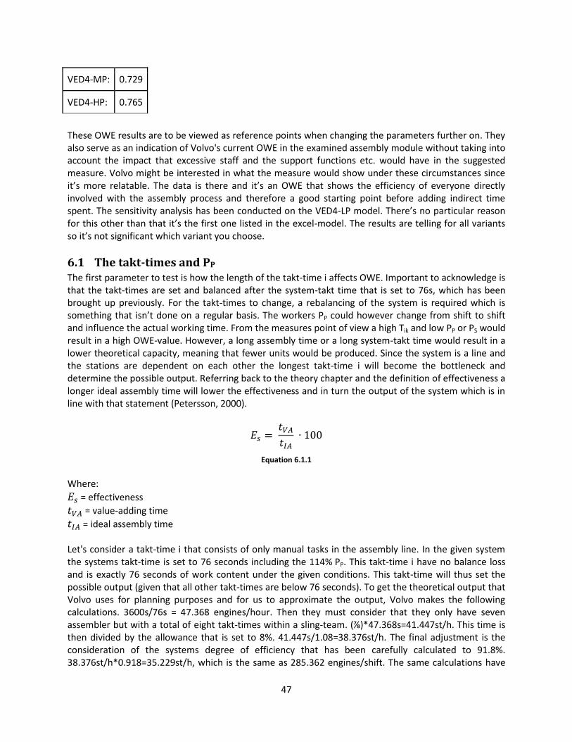
47

These OWE results are to be viewed as reference points when changing the parameters further on. They also serve as an indication of Volvo's current OWE in the examined assembly module without taking into account the impact that excessive staff and the support functions etc. would have in the suggested measure. Volvo might be interested in what the measure would show under these circumstances since it’s more relatable. The data is there and it’s an OWE that shows the efficiency of everyone directly involved with the assembly process and therefore a good starting point before adding indirect time spent. The sensitivity analysis has been conducted on the VED4-LP model. There’s no particular reason for this other than that it’s the first one listed in the excel-model. The results are telling for all variants so it’s not significant which variant you choose.

6.1 The takt-times and PP The first parameter to test is how the length of the takt-time i affects OWE. Important to acknowledge is that the takt-times are set and balanced after the system-takt time that is set to 76s, which has been brought up previously. For the takt-times to change, a rebalancing of the system is required which is something that isn’t done on a regular basis. The workers PP could however change from shift to shift and influence the actual working time. From the measures point of view a high Tik and low PP or PS would result in a high OWE-value. However, a long assembly time or a long system-takt time would result in a lower theoretical capacity, meaning that fewer units would be produced. Since the system is a line and the stations are dependent on each other the longest takt-time i will become the bottleneck and determine the possible output. Referring back to the theory chapter and the definition of effectiveness a longer ideal assembly time will lower the effectiveness and in turn the output of the system which is in line with that statement (Petersson, 2000).

Equation 6.1.1

Where: = effectiveness = value-adding time = ideal assembly time Let's consider a takt-time i that consists of only manual tasks in the assembly line. In the given system the systems takt-time is set to 76 seconds including the 114% PP. This takt-time i have no balance loss and is exactly 76 seconds of work content under the given conditions. This takt-time will thus set the possible output (given that all other takt-times are below 76 seconds). To get the theoretical output that Volvo uses for planning purposes and for us to approximate the output, Volvo makes the following calculations. 3600s/76s = 47.368 engines/hour. Then they must consider that they only have seven assembler but with a total of eight takt-times within a sling-team. (⅞)*47.368s=41.447st/h. This time is then divided by the allowance that is set to 8%. 41.447s/1.08=38.376st/h. The final adjustment is the consideration of the systems degree of efficiency that has been carefully calculated to 91.8%. 38.376st/h*0.918=35.229st/h, which is the same as 285.362 engines/shift. The same calculations have

VED4-MP: 0.729

VED4-HP: 0.765

48

been done for different PP and used to approximate the TPR for different PP-levels. Expectedly, the calculated OWE is the same for all PP-levels since the relation between system takt-time and TPR will remain the same as presented in the table below.

PP: 80% 100% 114% 134%

System-tt : 108.3 seconds 86.64 seconds 76 seconds 64.66 seconds

TPR: 200.26 engines 250.32 engines 285.37 engines 335.41 engines

OWE: 59.6% 59.6% 59.6% 59.6%

These calculations simply illustrates that the OWE will remain the same if the theoretical capacity can be reached for every PP-level. The approximated TPR’s is just a way for Volvo to schedule production. The allowance is not always fully used and sometimes the system doesn’t experience any disturbances, then the output will increase. The deciding factor is the bottleneck takt-time which will determine the highest potential output of the system. In all the other cases a PP above 114% will lower the actual working time at a takt-time that isn’t the bottleneck, resulting in a worse OWE result than before and vice versa for a PP that is below 114%. This is in line with what was stated in the theory chapter about efficiency (Petersson, 2000):

Equation 6.1.2

Where: = efficiency

= ideal assembly time = total work time The assemblers/workers are to be kept busy for as much of the total work time as possible, i.e. high utilization of the workforce, in order to reach a high efficiency. The discussion about Ps is the same as for PP, except PS is only moving between 100 % and lower. In the end it boils down to balancing the work content of a takt-time i to equal the systems takt-time. The PP comes in as a way to explain the reality of the system and the fact that assemblers perform at different speeds. The workers expected performance is set in relation to MTM-100 and serves as a way to balance the line and the work content to equal the systems takt-time, and at the same time be at a reasonable pace for the average worker. To analyze the impact of the PP requires more in depth knowledge of the production system and revolves around the bottlenecks. If a worker increases his/her working speed at a bottleneck, the output is increased. If the speed is increased at a takt-time i or assembly-sling that isn’t the bottleneck, the output will be unchanged and the OWE will decrease because of more waiting time for the worker being finished earlier. The impact of PP on TPR and OWE have been investigated further by collecting all the takt-times i for the different assembly slings for the VED4-LP variant. This allows the analysis of which slings that can increase the output by increasing their performance. This approach could be taken even further by decreasing and increasing the PP for every takt-time i, so that all takt-times i equals 76 seconds. This

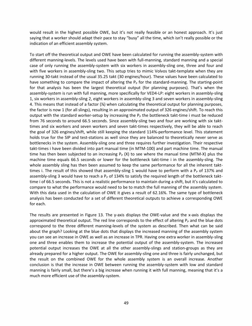
49

would result in the highest possible OWE, but it’s not really feasible or an honest approach. It’s just saying that a worker should adapt their pace to stay “busy” all the time, which isn’t really possible or the indication of an efficient assembly system. To start off the theoretical output and OWE have been calculated for running the assembly-system with different manning-levels. The levels used have been with full-manning, standard manning and a special case of only running the assembly-system with six workers in assembly-sling one, three and four and with five workers in assembly-sling two. This setup tries to mimic Volvos takt-template when they are running 30-takt instead of the usual 35.25 takt (30 engines/hour). These values have been calculated to have something to compare the impact of altering the PP for the standard-manning. The starting-point for that analysis has been the largest theoretical output (for planning purposes). That’s when the assembly-system is run with full manning, more specifically for VED4-LP: eight workers in assembly-sling 1, six workers in assembly-sling 2, eight workers in assembly-sling 3 and seven workers in assembly-sling 4. This means that instead of a factor (⅞) when calculating the theoretical output for planning purposes, the factor is now 1 (for all slings), resulting in an approximated output of 326 engines/shift. To reach this output with the standard worker-setup by increasing the PP the bottleneck takt-time i must be reduced from 76 seconds to around 66.5 seconds. Since assembly-sling two and four are working with six takt-times and six workers and seven workers and seven takt-times respectively, they will be able to reach the goal of 326 engines/shift, while still keeping the standard 114%-performance level. This statement holds true for the SIP and test-stations as well since they are balanced to theoretically never serve as bottlenecks in the system. Assembly-sling one and three requires further investigation. Their respective takt-times i have been divided into part manual time (in MTM-100) and part machine time. The manual time has then been subjected to an increasing PP (X) to see where the manual time (MTM-X) plus the machine time equals 66.5 seconds or lower for the bottleneck takt-time i in the assembly-sling. The whole assembly sling has then been assumed to keep the same performance for all the inherent takt-times i. The result of this showed that assembly-sling 1 would have to perform with a PP of 137% and assembly-sling 3 would have to reach a PP of 134% to satisfy the required length of the bottleneck takt-time i of 66.5 seconds. This is not a realistic performance to maintain during a shift, but it’s calculated to compare to what the performance would need to be to match the full manning of the assembly system. With this data used in the calculation of OWE it gives a result of 62.16%. The same type of bottleneck analysis has been conducted for a set of different theoretical outputs to achieve a corresponding OWE for each. The results are presented in Figure 13. The y-axis displays the OWE-value and the x-axis displays the approximated theoretical output. The red line corresponds to the effect of altering PP and the blue dots correspond to the three different manning-levels of the system as described. Then what can be said about the graph? Looking at the blue dots that displays the increased manning of the assembly system you can see an increase in OWE as well as an increase in TPR. Having one extra worker in assembly-sling one and three enables them to increase the potential output of the assembly-system. The increased potential output increases the OWE at all the other assembly-slings and station-groups as they are already prepared for a higher output. The OWE for assembly-sling one and three is fairly unchanged, but the result on the combined OWE for the whole assembly system is an overall increase. Another conclusion is that the increase in OWE between running the assembly-system with low and standard manning is fairly small, but there’s a big increase when running it with full manning, meaning that it’s a much more efficient use of the assembly-system.

50

Figure 13 Graph displaying OWE(y-axis) and the theoretical output(x-axis) for different manning levels(blue) and the effect of

altering PP for standard manning(red)

The effects of altering the PP for the bottleneck-slings are similar but OWE is lower for the same theoretical output. This has to do with the effects that an increased working speed has on the OWE for the bottleneck slings. The part machine time is unchanged, but the part manual time is decreasing as an effect of the increased working speed. This effect outweighs the effect that the higher number of potentially produced engines has on the total time spent by the worker and in turn results in a lower OWE. OWE at the other station-groups is the same as in the case with the increased manning scenario. Overall it can be stated that it’s more efficient to run the assembly-system with full manning rather than increasing the speed at selected bottlenecks. By working with fully manned assembly slings the new potential output requires all station-groups to work at full pace and fully utilize the time spent in the different station-groups (not considering the balance losses). However, referring back to what has been said previously, the choice to have an open spot in an assembly-sling can be beneficial. It’s put there, in Volvos case to allow some space in the sling and to serve as a leveling buffer. The system is more exposed to disturbances if it’s working at full capacity as a stop somewhere in a sling will pause the production of all other takt-times i within that sling. To run the system with full manning is also a matter of cost which has to be taken into consideration. That is where this type of analysis really can be a helpful tool. By analyzing how an increased PP can increase the potential output of the system you can actively boost the performance of your production system by making active choices. This could for example be done by rearranging the workers to have the ones that can work faster at the bottleneck-slings. However, to fully utilize this and make informed decisions more data would need to be collected. As brought up in a previous chapter a good way to acquire the necessary data would be to start measuring the actual assembly time for the takt-times i and store them. This would preferably be done through the use of manufacturing execution systems that can log this type of data. This data would enable Volvo to constantly measure and compare the set performances and the actual performances. Even if a PP of 137%, as used in the graph, might not be a realistic performance-target the full spectra of achievable PP is interesting. To achieve a potential output of 293 engines the performance of sling one needs to be 118% and the performance of sling two needs to be 117%. This is more reasonable or achievable. This might not even happen because it was set out as a goal, but the workers had a good day and experienced a sense of urgency, resulting in a higher

0.59

0.595

0.6

0.605

0.61

0.615

0.62

0.625

0.63

0.635

230 250 270 290 310 330 350

Manning

Pp

51

performance. The PP could be monitored for a bottleneck, whether it’s a single takt-time i or for a whole assembly sling. This would help with investigating where there’s improvement potential within the system and to explain good or bad results. A possible scenario could be that the takt-time i, through the development of new methods by the worker can be performed faster than anticipated, given that the manual time should be MTM-114. A fairly skilled worker is constantly performing over the set performance-target with relative ease. Instead of this knowledge getting hidden within the assembly-system it can surface more easily. The takt-time i can then be rebalanced or adjusted after what should be the MTM-114 performance instead. It also builds knowledge of the workers performance. Even if it’s not custom in today's industry to have different pay for the same job, a salary raise for increased performance is something that could potentially be beneficial in the future if both parties could come to an agreement. This can be used as a tool for achieving output flexibility for the assembly-system. Obviously you wouldn’t have workers performing MTM-137, but just a slight performance boost could increase the potential output. You could also track PP for a sling and see if there is a connection between the PP and the number of disturbances in a sling. A higher pace could potentially make the workers more likely to commit mistakes. As explained earlier, the TPR used here is a calculated potential output. If there are no disturbances and the allowance isn’t fully used, it could be higher. That’s why Volvo themselves needs to collect more data to see how these variables affect the real output. Moving on, let’s instead look at how the OWE-measure changes with different values of TPR when the PP and PS is unchanged.

6.2 Total Parts Run Theoretically TPR (standard manning) can reach: 3600/76=47.7st/h, (⅞)*47.7st/h=41.5st/h, or 41.409*8.1= 335.41 engines/shift, which is the maximum amount of engines produced per hour when there’s no disturbances and none of the allowance is used. To achieve a higher output than this have been deemed unlikely since that would require all bottleneck takt-times to go below 76 seconds. The theoretical output they use for planning purposes, calculated previously, is 285.37 engines/hour. However, the TPR can sometimes go below this because of scheduled personnel not showing up, quality issues, difficulties with keeping the takt-time etc. The starting value for TPR has therefore been set to 241 engines/shift. Since the expected output of 286 engines/hour already have compensated for downtime and allowance it is unlikely that the TPR will be much lower than that, given that the system is producing at the highest takt according to Volvos takt-template. The starting value was still set to the fairly low value of 241 engines/shift to cover a larger interval and the effect on OWE by some really poor potential results. The result of how OWE changes with different TPRs in intervals of 15 is presented in figure 14. On the x-axis a range of different values for TPR is displayed and on the y-axis the corresponding OWE value is displayed. Comparing the default TPR of 286 engines/shift an increase to the highest potential TPR of 335 engines/shift will mean a 14% increase of the OWE going from 59,80% to 68,35%. This target is unlikely to reach since it would mean zero disturbances and no utilization of the allowance. For a smaller shift in TPR moving from 286 engines to 301 engines the difference in OWE is an increase of 4.30%. For a decrease in TPR from 286 engines to 271 engines the difference in OWE is a decrease of 4.43%. The relation between OWE and TPR seems to be approximately linear for the given interval, which is also the only relevant one. TPR-values above 335 engines would mean a shorter system takt-time and a value below 241 engines or less would mean that something is wrong with the system and give skewed OWE results that are mainly caused by major disturbances.

52

Figure 14 Graph of how OWE changes with TPR

6.3 Planned Down Time The planned down time is the time when the system is scheduled to not produce and thus that time isn’t weighing down the OWE. The PDT for a single shift is rarely that high though, but in the graph it ranges from one minute to half an hour with a five minute interval between each data point. The result is visible in figure 15. The x-axis shows the PDT and the y-axis shows the OWE. The relation between the two seems to be linear in this case as well. Moving from a PDT of one minute to a PDT of half an hour the change in OWE is a 5.61% increase in percentage points which could be seen as fairly large. The likeliness of Volvo having a PDT for half an hour for a single shift is however fairly unrealistic. The fact that a shorter working time would also mean less engines produced could also eliminate the increase in OWE. According to Volvo's takt-template they produce an engine every 101.96 seconds. If the PDT is 1800 seconds, that’s 1800/101.96=17.654 engines that won’t be produced resulting in a TPR of 286-18=268. This TPR with the given PDT of 1800 seconds results in an OWE of 0.5991 which is more or less the same as with a PDT of zero.

Figure 15 Graph of how OWE changes with PDT

0.5193 0.5454 0.5715 0.5976 0.6237 0.6498 0.6835

0

0.3

0.6

0.9

241 256 271 286 301 316 335.41

OWE-TPR

OWE

0.5987 0.6031

0.6087

0.6144

0.6203

0.6262

0.6323

0.58

0.59

0.6

0.61

0.62

0.63

0.64

60 300 600 900 1200 1500 1800

OWE-PDT

OWE

53

6.4 Over and/or understaffed How does OWE change if the line is understaffed? This is not the same as in figure 13 where the different manning-levels of the assembly-system were investigated. This is if the assembly-system is operating with fewer workers than stated in the takt-template. This is complicated to visualize in a single graph since it matters where you withdraw a worker. If it’s at the SIP, there must be a worker there, if not, the flow stops. If it’s at one of the assemble-slings they can operate as usual, but with a lower output. Let's assume that the first assembly-sling operates with six instead of seven workers. Practically this isn’t the case, because if a worker is absent the team leader of that sling can fill in, but let’s calculate the OWE for theoretical purposes. This loss in manpower would mean a lower output from the assembly-sling and serve as a bottleneck for the rest of the system. As the theoretical output that Volvo uses in their takt-template was compensated for seven workers with eight stations, it must now be compensated for six workers with eight stations resulting in an approximated TPR of 245 engines during a shift. This would result in an OWE of 54.13% compared to the default OWE of 59.76%. However, with more space in the first assembly-sling, the assemblers there could potentially pick up the pace and work faster. If the assembler in front is finished quicker and move forward to the next station, there’s a gap to fill if the assembler behind also is done. The team-leader of the sling can also put in more work in the line if required, as they are more flexible in their time spent assembling. Let’s assume that this understaffed sling can still reach the planning target of 286 engines during a shift, which theoretically is possible disregarding the allowance and the systems degree of efficiency. That would result in an OWE of 61.46%. Production engineers have voiced concerns for these types of results. That the best OWE results are being reached when they are understaffed and that it’s a discouraging measure if the result of the measure gets better when people call in sick or doesn’t show up. However, production targets are set with disturbances and allowance accounted for. If there’s no disturbances and the allowance isn’t used e.g. because of a sense of urgency emerging from being understaffed, the target could still be reached. Add to that the potential increase in PP for the affected assembly-sling and there are various reasons for achieving or not achieving a certain output. All these circumstances and parameters must be taken into account when judging an OWE result. If the output target can be reached with fewer assemblers, maybe there is an efficiency problem? What circumstances caused it? Was the output target reached through fewer breaks, no disturbances and an increased working pace? Then that might not be a sustainable way of working in the long run, but if the same output can be reached with a smaller workforce without any special circumstances a thorough investigation about inefficiencies in the system should be made. A more direct way to investigate the impact on OWE is for the overstaffing of the assembly line. The praxis is that Volvo schedules more workers than necessary to minimize the risk of running the assembly understaffed. The downside to this is that they often have more workers present than what is necessary for standard production. These extra workers will impact OWE negatively and this impact can more easily be displayed in a graph than for the previous case of understaffing. Included in the number of excess workers can also be ICA-personnel or other workers present that isn’t part of standard production. In terms of the measure it just adds more man hours to the denominator. Figure 16 displays of how OWE changes with an increasing number of excess workers. The x-axis shows the increasing number of excess workers, whether it’s extra assemblers in the line or ICA-personnel, and the y-axis shows the OWE.

54

Figure 16 Graph of how OWE changes with excessive staff

For two excess workers the OWE decreases by 5.27% from 59.76% to 56.61%. The relation once again seems linear and for the final value of seven excess workers there has been a decrease from the default OWE value by 16.28%. This could be a possible scenario considering occasions were ICA-personnel have been called in on top of regular overstaffing. This have a big effect on the OWE which should serve as a tool to keep the workforce under control. Petersson (2000) states that only using the required number of assemblers in a process force them to work at full pace, as the system should be designed for use at the theoretical capacity. This in turn will make a ramp-up of the assembly rate easier as the existing assemblers are used to working at full pace (Petersson, 2000). Having excess workers in a line or assembly system could also hide the shortcomings of it, compensating with excess workers. This can hide the waste of the system that would otherwise surface, besides excess workers being a source of waste itself (Shah & Ward, 2007).

6.5 Truck Drivers This will be a short section about the impact of the two truck drivers that exists as rotational spots for the assemblers in the system. In the default OWE value they are considered value adding (defined as the time they spend driving) 80% of their total working time. A fair option would be to consider them non-value adding or not part of the line, since they are only supplying the line with material, but not part of the flow. This would change the OWE to 55.31% which is a 7.45% decrease from the default OWE. This is a significant change and it’s up to Volvo to decide on how to handle their added time. How much of it should be considered value-added, if any, or should they be excluded from the model completely?

6.6 Engine Adjustment The time spent at Engine adjustment by workers is subtracted from the numerator. As argued for previously this amplifies the negative effect that quality issues have on OWE. Unfortunately, no good data have been obtained on how many hours/seconds that is spent there per shift. At the function they handle faulty engines from all the assembly lines so it’s a bit difficult to trace the time specifically spent on engines from the assembly line of interest. Because of this a lot of data points for the time spent at Engine adjustment have been added to help see how OWE changes over a larger interval. The idea of this is to help Volvo with evaluating how OWE changes depending on the time that is spent at Engine

0.5976

0.5814

0.5661 0.5516

0.5378 0.5247

0.5122 0.5003

0.44

0.46

0.48

0.5

0.52

0.54

0.56

0.58

0.6

0.62

0 1 2 3 4 5 6 7

OWE-Excessive Staff

OWE

55

adjustment. The exact amount of time spent on engines from the assembly line of interest is something they can look into themselves at a later stage. Figure 17 displays how OWE changes with an increasing number of time spent in the Engine adjustment function. The x-axis shows the time spent on engines from the assembly line of interest by workers at the Engine adjustment function. The time is stated in seconds. The y-axis displays the OWE.

Figure 17 Graph of how OWE changes with an increasing amount of rework

The relation between OWE and the total time at Engine adjustment (EA) is not linear. Only a few data labels have been made visible in the graph to illustrate the change. The first one displays an OWE of 59.58%. This result is had with an EA of 1822 seconds, or about half an hour. The next data label shows an OWE of 59.20% with an EA of 5832 seconds, or about 97 minutes. Still the decrease in the result of OWE is fairly small, but on the other hand, so is the EA. The next data label that displays an OWE of 58.37% corresponds to an EA value of one employee working for half a shift. For one worker in Engine adjustment working for a full shift the OWE drops from the default value of 59.76% to 56.98%. That’s a 4.65% decrease which is quite significant. The next two data labels of 54.20% and 50.04% correspond to two full time workers and three and a half respectively. The point being that the OWE is heavily impacted by an increase in workers doing full shifts at the Engine adjustment function. Rework and quality issues should of course always be avoided and Volvo most certainly has performance measure that monitors quality already. To reduce rework is more related to continuous improvements, good product design and stable assembly processes, not so much to the single workers having to concentrate on a daily basis to be error-free. Methods that reduces or completely eliminates the risk of making faulty assemblies is instead important to have in place (Shah & Ward, 2007). However, the OWE measure should incorporate the impact of quality issues and rework, since it’s connected to the workers and their efficiency. That is the ones performing the actual assemblies on the engines and the ones having to troubleshoot and correct their potential errors. Sometimes it’s not the assemblers fault, as it could be the material or the added parts that have been delivered with quality that doesn’t reach the specifications. Nevertheless, that’s for other improvement initiatives to help correct and eliminate. Another reflection about the measure and the impact of EA is if the rework activity can be done within the assembly line instead of moving it to a separate function. That would mean reducing the EA and instead taking up more of the total working time in the assembly line and potentially reducing the output (TPR). Reducing the output slightly would have a less negative impact on the result of OWE than

0.5958 0.592 0.5837 0.5698

0.542

0.5004

0.4

0.45

0.5

0.55

0.6

0.65

OWE-EA

OWE

56

spending that time in the Engine adjustment function (Petersson, 2000). To conclude this section some final reflections on the impact rework has on the result of OWE will be made. The impact it has is by design and it is up to Volvo to make a decision about its inclusion and the current state of the formula used for calculating OWE. An alternative could be to exclude it completely, but based on previous explanation the quality, and by extension the rework, could be seen as important to incorporate into OWE. Nevertheless, it could be regarded as separate things. OWE could be concerned with keeping track of the efficiency with a heavier focus on utilization, while rework could be monitored by the quality function and other performance measures. Another practical issue is that it could be seen as complicated to keep track of how many man hours are spent on faulty engines from a specific line or module. However, the total man hours spent should already be kept track of somewhere and it wouldn’t necessarily mean that much more work to sort it into categories. The information of the distribution of engines that requires rework should also be interesting to keep close track off and from which assembly line they come. If it’s complicated to compile per shift an adequate approximation would be to gather that data for a month and then divide it by the total shifts per month.

6.7 Support Functions including team-leaders and managers The addition of the time spent by support function will impact the OWE in the same way that adding the time for the excess staff did. The difficult question is to decide which functions and their respective activities that should be included. This could make up an entire thesis on its own. Keeping track of all the networks of activities and the time spent on them is no end in itself and the data collection and storage should be carefully thought out. The main goal of incorporating support functions is to surface potential wastes and inefficiencies. To keep an assembly line running, what support functions needs to perform supporting activities? This reaches beyond the development of a new measure of worker efficiency and would include a detailed analysis of the components that make up these processes. The complexness of the process is further increased by the involvement of manual labor that is characterized by a larger degree of variation than the automated counterpart (Wheelwright & Clark, 1992). It all basically boils down to the challenge of achieving a higher degree of process control. The difficulty with larger organization is that they get increasingly hierarchical and divided into their separate functions and areas (Wheelwright & Clark, 1992). This can make gaining a higher degree of process control more difficult since different functions are acting after their own budget and have their own targets. To achieve an overview can therefore be easier in a smaller company since they have a clearer picture of the company as a whole. To achieve this in a large company such as Volvo the formation of a cross-functional team with representatives from the concerned functions is common practice and would be a good start for an undertaking like this (Wheelwright & Clark, 1992). In chapter 4.3.6 the relevant support functions for the assembly line of interest was identified. The next step would be to identify the performed activities of each function that are related to the running and maintenance of the assembly line and somehow rank them in order of importance and how much time is spent on them. Obviously some sort of prioritization should be done to exclude insignificant activities and/or infrequent activities in order to lower the complexity and data collection/storage. When the activities have been identified an approximation of the time they take to perform should be made. This could be done in a similar fashion to the TD-ABC costing method. Some sort of costing methodology is certainly already in place to help with budgeting, as with any large company. To calculate the unit cost is however not the main objective in this case. It’s more about keeping track of the man hours spent, although they are related. How many man hours in total are spent running the assembly line? This is definitely related to the overall worker efficiency and the rationale is increasing the process control by making the hidden, or rather indirect man hours visible. This has been deemed even more crucial in a start-up phase of e.g. a new process. If the resources required for such a rigorous process control isn’t justified for everyday production it could be

57

done exclusively for the introduction of new processes. Excessive manning and costly indirect activities can become standard practice if they are employed initially to help with start-up problems. That’s why it could be beneficial to have an increased transparency in a start-up phase. Figure 18 displays how OWE changes with an increasing number of time (in seconds) spent by support functions. The x-axis shows the time spent by support functions and the y-axis shows the OWE.

Figure 18 Graph of how OWE changes with an increasing amount of time spent by support functions

Included in this demonstration are two of the manager positions that were excluded from the calculation of the default OWE. It’s the position of supervisor and superintendent. With these two and their time spent included as a support function OWE decreases from 59.76% to 58.74%. After this the time spent increases by 29160 seconds (a full time worker for a whole shift) to act like a steady increase in time spent by regular support functions. As mentioned in the beginning of this section, OWE will behave in the same way as adding time for excess staff and the graph would be identical if they time for the managers weren’t included. The OWE value of 49.31% corresponds to the time of seven employees working for a full shift and the two extra managerial positions. The number of seven is just used to illustrate how OWE could change when adding the time that support functions spend on activities related to the assembly line. How much time support functions spend in reality is not known and haven’t been investigated. Considering the fact that a large number of employees could be involved it could also be considerably higher. However, the time spent by the single support function worker should be relatively low for the single shift. This would make the total time spent by all support functions comprise of a large number of workers adding small portions of time spent, which is probably the case. All in all, this final reflection was mostly about stating the background for the numbers used and point out where the assumptions might be flawed. The usage of the measure would however still remain the same regardless of the result. Although a very low OWE result because of adding support functions would probably intimidate managers from implementing and using such a measure. Further investigation by Volvo on the time spent by support functions is needed.

0.5976 0.5874

0.5718 0.557

0.5429 0.5295

0.5168 0.5047

0.4931

0.4

0.45

0.5

0.55

0.6

0.65

OWE

OWE

58

7 Discussion

This chapter provides the discussion of the thesis. In the first section the suggested OWE-measure is compared to other measures brought up in the theory-chapter. The next section discusses how the results of the study can generalized and applied to assembly-systems with a varying range of automation. This is followed by a section on how OWE can be used in a ramp-up phase. The final section brings up a general discussion about the results of the thesis.

7.1 The suggested OWE-measure compared to others

To begin this discussion the proposed OWE measure will be compared to already established versions of worker efficiency/effectiveness measures. The first definition of OWE and a good starting point is Volvo's own definition, included in their loss-model. They state that: OWE = Value-added man hours / Total man hours. This is more or less what the proposed measure is stating as well. It’s just a concrete way of actually measuring it. The loss-model states that “Total man hours” consists of both white collar and blue collar workers, which the proposed measure includes through the addition of support functions. The losses mentioned are Excessive manning losses, Management losses, Balancing losses and Non-value-added direct work losses. The first one is included in the proposed measure through accounting for the number of excessive workers in production and the added time that managers spends managing the assembly-system of interest. The Management losses or rather Organizational losses, are also included through the addition of time added by various support functions in the proposed measure. The Balancing losses are also taken into account by using the data for every takt-time i, where the balance losses are directly visible. Then that takt-time i gets subjected to PP and PS to see how the individual's performance can increase or decrease that balance loss, resulting in the actual balance loss. Non-value-added direct work losses are added to the proposed measure by including VA in the formula. The difficult part about that procedure is defining what part of the time spent is value adding and which parts are not. This leads to difficult decisions when categorizing tasks and activities. This loss-category is also included in the proposed measure through the subtracting of the rework-time in the numerator. This is a choice made to have quality-issues affecting the proposed measure more severe. Overall the proposed measure is deemed as a close fit to Volvo’s definition of what OWE should be. It’s boiled down into an actual measure, where practical choices were made in order to achieve usability and clearness of the proposed measure. The next alternative OWE measure to compare the proposed measure to is OLE, or Overall Labor Effectiveness. This measure strives to mirror the machine-counterpart measure of OEE. It’s divided into the three factors Availability, Performance and Quality and then multiplied for a cumulative effect. The factors with their respective calculations are as follows: Availability = Time operators are working productively / Scheduled time. Performance = Actual output of the operators / the expected output. Quality = Saleable parts / Total parts produced. This is a rather simple way of approaching the topic of worker efficiency/effectiveness. The input parameters are vaguely defined and kept fairly simple. This measure is more along the lines of a generic management tool. The conclusions that can be drawn from the factors and their cumulative result are limited. The company behind OLE instead puts emphasis that these factors are being subjected to further analysis through their Workforce Analytics-tool. This tool will then help with diagnosis and finding the “root-causes” of potential problems. For example they state that problems with Performance can be related to poor training and skills for the employees (Kronos, 2007). This would then translate into less output for the workers, resulting in a worse Performance-factor. However, in the proposed measure of this thesis the single takt-time i is being accounted for and worker j’s individual PP and PS is

59

also incorporated into the OWE-measure which directly impacts the result of OWE with visible cause and effect, at least regarding that issue. The diagnosis and root cause-analysis is necessary anyway, regardless of the measure, but the OLE-measures definition of factors could be regarded as over simplified. A company like Volvo, as well as other larger, more mature companies operating in the forefront of performance measures should question themselves if simple is what they really need. Also for this measure the idea of support functions adding time is disregarded. It could be that it’s included under Availability, where they could be included under scheduled time for certain tasks. Again there’s an ambiguity issue with the OLE-measure. The final measure to compare the proposed measure to is the MAE-measure developed by Petersson (2000) as an attempt to fill the void at the time present for process efficiency measures for manual assembly. This void is still to be filled by a measure that’s widely used and accepted within the industry and that’s where the proposed measure comes in as a proposition. The two shares many similarities since the starting-points have been more or less the same and Petersson’s work have been an inspiration. Petersson chose to use the Ideal assembly time for unit i instead of dividing it into the single takt-times i of the unit of interest. The division of the Ideal assembly time into its components enables the analysis of subparts of the system, as well as it can specifically highlight the takt-times i that are the most inefficient. Added to this is the concept of including PP and PS which affects the time that takt-time i actual takes. Peterssons OLE doesn’t take into account that the tIAi might differ from the actual assembly time for unit i. This might be because of the workers working faster, or new found methods to perform the tasks quicker. Regardless of cause, it enables a higher process control to be aware of it and actively monitor it. The decision to subtract the time for rework from the numerator of the proposed measure was a result of Peterssons (2000) argumentation of it impacting the measure more negatively that way, promoting quality as an important issue. The denominator of MAE is similar to the proposed measure, but structured in a more simple way. The number of assemblers are multiplied by their scheduled time minus total planned stop time and total unused assembly time due to lack of orders. The proposed measures summation of workers allows for different scheduled times for different workers. Also the unused assembly time due to lack of orders has been neglected in the proposed measure. The rationale for subtracting it in MAE is that the efficiency of the system should only be measured for the time it’s being used. The argument for not subtracting it in the denominator is that if workers are still present, salaries are being paid and that would be an inefficient use of the assembly-system. The assembly-system should be the entity that’s adapting after the demand and thus give a bad OWE-result if it fails to do so. The biggest difference between the two measures is that the proposed measure can include support functions and excessive manning while MAE disregards this aspect. This could arguably be seen as a potential big source of waste and something worth investigating further. The proposed measure has the ambition to widen the scope for what should be included in a worker efficiency measure. A strength of the proposed measure is that it can be scaled, as done in the created excel-model. You can measure the OWE for a single assembly-sling and only focus on the efficiency of the assemblers working there. It can, and should however be possible to view the whole picture. This is achieved by adding hours spent by support functions, the excessive manning etc. The consideration and inclusion of VA is also a step to align the proposed measure with Volvo’s perception of OWE and the wastes within manual assembly.

7.2 How can the results be generalized and how OWE can be applied to

automated lines From the outset the purpose of the thesis was to develop an overall worker efficiency KPI for Volvo cars specifically. However, the ambition was also to develop a measure that can be generally applied within

60

the industry. As some of the components of the proposed measure are specifically addressing functions residing at Volvo it could cause some doubts for generalizability. Most of these cases are just a question of what you choose to name the different parameters. The total time at Engine adjustment is just the time spent on rework and easily translates into other industries. The time for truck drivers can be removed if none are present and the inclusion of white collar workers can change depending on what support functions are active within the company of interest. The core of the formula will remain the same regardless of that. What’s left to do is to investigate the network of supporting activities and the time spent by them and managers and other white collars. The idea of excessive manning is also something that is easily applied to other companies, and is of course nothing that Volvo exclusively deals with. However, to claim that the results are generalizable and externally valid from a research perspective is not correct. Instead, as described in the method chapter the reader must make the judgments based on thick descriptions about what is possibly transferable into other contexts. Another interesting aspect is the application area of the OWE-measure. It covers both manual and semi-automatic systems. This means that the system can include both manual and fully automatic processes, in other words a combination of the two. An interesting area is the middle of the spectra and when the systems are more automated than there are manual work tasks to perform. This could lead to a combination of using both OEE and OWE.

Figure 19 The application area of OEE and OWE by Petersson (2000)

These types of scenarios are increasingly becoming a reality within today’s industry and many companies are uncertain on how to handle worker performance measures in those situations. The proposed measures division of manual time and machine time is something that could help with bridging that gap. Acknowledging that the worker is unable to influence the time a machine takes to finish and that his/her time spent idle leads to a lower OWE is key in painting the whole picture, and in turn making informed improvement decisions. A further development of the proposed measure is to continue the division of the parts that make up the total takt-time i. For the proposed measure only the manual time of takt-time i at sling-team k is considered, but the following approach could be interesting:

Equation 7.2.1

Equation 7.2.2

= the total takt-time

= the part machine time = the part manual time

61

= the part of the machine time where the operator is occupied

= the part of the machine time where the operator is unoccupied

The machine time can be divided into if the operator has to oversee the machine (occupied) or if the operator is idle when the machine is running (unoccupied). Tunoccupied can be used to increase the OWE instead of keeping it as pure machine time. This is already how Volvo is approaching the work content performed at their Test-stations. They have three machines running in parallel with the worker moving in between performing the manual tasks and thus eliminating as much as possible of his/her own idle time. In the case of a worker having more of a surveillance role, overseeing a big automated process, it’s harder to obtain a good OWE-result. However, a low OWE in comparison is not necessarily a bad thing. The most important thing is how the measure detects means for improvement, which the division of machine time into Toccupied and Tunoccupied does (Andersson & Bellgran, 2015). This approach to OWE and the extended division of machine time opens up for interesting combinations with OEE which could be the topic for future research. Another insight about OEE is that it’s supposed to measure individual equipment efficiency, but is in fact affected by the surrounding environment which has been concluded by several researchers (Hedman et al, 2016; de Ron & Rooda, 2005). Included in the surrounding environment is among other things, how the operators can influence the result of OEE. Hedman et al (2016) analyzed this and came to the conclusion that in order to improve equipment efficiency, the supporting activities performed must be the right ones. The planning and execution of these activities are key for reaching a higher level of efficiency (Hedman et al, 2016). In their analysis they found that 90% of the recorded downtime (of the losses they could categorize) could be directly related to the supporting activities performed by the operators, and not caused by the automatic process itself. A way to work with these types of system in the future could be to view OWE and OEE in relation to each other and try to maximize the system’s efficiency. A way to do this in a semi-automated system is to increase the decision basis for the operators in order for them to be able to make informed decisions. It could revolve around performing service on a machine or refilling material, and in which order the tasks should be performed to minimize downtime to achieve the highest possible efficiency (Hedman et al, 2016). The focus between OWE and OEE shifts depending on the classification of the assembly systems. If it’s more towards an automatic system OEE would be given priority and vice versa. It’s a question of priorities and what is most cost efficient. A high utilization of the working operators is not as important in a highly automated system with expensive investments in equipment and machines. Then it’s more about how to handle certain situations and making informed decisions to guarantee that the process isn’t stopping or not running at full capacity, as was stated previously. In a manual assembly line the OWE-measure gets increasingly important to make sure that the system is well balanced and that all workers are utilized in an efficient way.

7.3 Utilizing OWE in a ramp-up phase In the introduction of this thesis the risk of excessive manning in a ramp-up phase is brought up. The identified issue with this is that the temporary increased manning level can be prolonged and later become permanent, resulting in a more inefficient production system. This chapter will cover how the proposed OWE-measure can be used to identify and assist with this and other types of inefficiencies experienced in a ramp-up/start-up phase. First off the proposed OWE-measure addresses the risk of excessive manning by keeping track of the number of excessive workers and ICA-personnel present in the assembly line. In a ramp-up phase the production system might experience issues where extra staff and ICA-personnel are required to be

62

present. However, when these issues are solved the production system should go back to using the required to operate level of manning again. A default OWE-result could be set for the newly designed production system with the default level of manning. As the ramp-up phase commence the actual OWE-result will probably be lower, but as the production system reaches maturity and standard production, the OWE-result should move closer to the set default-value of the production system. An issue here is to approximate the hours spent by support functions and other additions to the proposed OWE-measure in order to set a default value. This can be handled by only looking at OWE for the production system itself and the excessive manning and ICA-personnel, much like equation 5.3.5.1 presented in chapter 5. This is a simple way of monitoring the manning levels of the system and to follow the trend of OWE as the production systems enters the maturity face. In a similar fashion the proposed OWE-measure can be used in a ramp-up scenario for keeping track of the identified support functions. This can be beneficial in two ways, both before and after the implementation of the newly designed production system. Incorporating the support functions into the OWE-measure requires an investigating of the support functions that are involved in performing supporting activities for the production system of interest. The necessary supporting activities and the time spent on them could be assessed in a design phase, before the start of production. A method to aid with this could be TD-ABC as mentioned previously. This mapping of the supporting activities and the time spent on them leads to a higher process control and in turn a better chance at achieving a smoother ramp-up phase. It also enables a better cost approximation of the designed production system for budgeting reasons. Once the production system has been implemented and has reached the maturity phase an assessment of the time spent by support functions could be performed again. This assessment could be compared to the initial one. The potential changes in the time spent by support functions could be motivated, but it could also be the case of inefficiencies. This investigation can serve as a way to identify improvement potentials and also as a way to reflect on how these activities currently are structured and carried out within the organization. A final way to utilize the proposed OWE-measure in a ramp-up phase is to continuously measure OWE throughout the ramp-up phase for only the production system itself, much like equation 5.3.3.2 or 5.3.4.1 presented in chapter 5. This is a way to investigate the balance losses in an early stage where things are easier to adjust and rebalance. The part manual time of the takt-time i according to MTM-114 (or whatever the performance level is set to) can be compared to the workers actual performance. This is obviously impacted by the learning curve experienced when dealing with new working tasks, but the trend is interesting to follow. This can help identify if there are any changes to the stated methods of the work content at individual takt-times i.

7.4 General discussion of the results The analysis presented fairly low results for OWE. This is partly because the time considered is only the manual time of the total takt-time i. If a line is running with excessive manning and man hours for supporting activities are added as well the OWE-result will move down towards 50%. These types of results should not discourage managers from using the performance measure as a lower result means greater improvement potential. The inclusion of VA should however be done with care. For the analyzed variant the percentage of VA-time is around 50% for any given takt-time i, which would lead to OWE-results around 25-30%. This could potentially skew the results and make it harder to draw conclusions and clearly make visible the effect that other improvement initiatives might have on the assembly-system. The fact that the definition of what should be categorized as NVA, NNVA and VA is somewhat unclear and could be influenced by the will to increase the OWE-result makes it a difficult parameter to

63

include. Another issue concerning the result of the measure is its possible range. From a theoretical point of view you don’t want an efficiency measure to be able to go above 100% since the measure should indicate to what degree a given process is utilized in practice. To exceed or even reach 100% for the suggested OWE-measure is however practically impossible. Even if only the workers within the assembly-system were considered (no support-functions, managers, excessive staff etc.) they would have to achieve the theoretical maximum output of 29160 s/76 s=384 engines or above it. But reaching an even higher output would mean lowering the bottleneck takt-time and thus the relation between the time spent producing and total working time would remain similar. There are also the balance losses within the assembly-system to consider which make reaching an OWE-result of 100% close to impossible to achieve.

The sensitivity analysis suffers a bit from poor data. In hindsight better data regarding the output per shift with the distribution of the different variants and models would really enrich the analysis and the possible conclusions. However, this type of data wasn’t easy to obtain and was accessed through unintuitive databases where the different variants had names that required decoding to identify. The data is however there, but should be compiled and presented in a better way for use in the calculation of OWE. The corresponding manning of the system for the given output/shift is also necessary to have available, which complicated the data collecting process. The reason why the output of the shift in combination with the manning level is important for the analysis is that it would be interesting to see how well the system is running with the different manning levels. Data concerning the time spent by support functions was not collected for this thesis. This is something that Volvo will need to investigate further. An interesting aspect to consider regarding that topic is not only the time that each support function spends, but if the cost associated with that time spent differs in comparison. The measure could potentially have the parameters be weighted differently to account for this. An example could be if the cost for having ICA-personnel present in production is considerably more expensive than having standard excessive staff there. These sorts of issues must be considered for the future development of the measure. On the topic of the sensitivity analysis and its discussion of PP and how it could be increased to achieve a higher potential output it could be interesting to have a discussion about social sustainability. The social sustainability is one of three common elements of sustainability where the other two are environmental sustainability and economic sustainability. The social sustainability within businesses is regarded as a business that meets the expectations of stakeholders without causing harm to the well-being of society and its members (Lindgreen et al., 2009). It’s concerned with business operations and the effects they have on employees, suppliers, customers etc. The concern is that workers might come to harm when setting unreasonable PP-levels or causing them stress when measuring their performance. Volvo can’t set these performance targets as they please, but there has to be an agreement with the workers and unions. Another issue related to social sustainability is equality and social diversity. The performance targets set for the average worker must be attainable for both female and male workers and the ergonomics must be adapted for everyone's physique. It’s important to be aware of these issues when dealing with measuring of actual people. It’s also important to inform the workers on how the collected data will be used and not cause them emotional stress since that would not be a sustainable working environment.

64

8 Conclusion

The purpose of this master thesis was to develop an Overall Worker Efficiency KPI for Volvo Cars that could also be generalizable for the manufacturing industry. For this conclusion the research questions that helped break down the purpose into smaller parts will be answered. RQ1: How can an organization such as Volvo benefit from introducing an OWE-measure? As with many other performance measures the OWE-measure will help Volvo identify improvement potentials. By better keeping track of the hours spent by employees they will reach a higher level of process control. This in turn will surface the potential wastes currently within the system. Acknowledging the time added by support functions and the number of excessive workers that are present in the assembly system will enable Volvo to have a more holistic view of how their operations are run. A measure like OWE will also encourage small improvements to the assembly system. Examples of this can be method improvements, rebalancing of takt-times and efforts of trying to decrease excess staff. Acquiring this holistic view of the assembly system is extra important in a start-up phase. Volvo wanted to use these new KPIs for production system development projects and in these early stages it’s important to eliminate waste as soon as possible. In the beginning the rules and procedures aren’t set in stone and are more easily subject to change. That’s why it’s beneficial to use this measure in a start-up stage. RQ2: What type of parameters does an OWE-measure need to contain and how should they be structured in order to be effective? The basic parameters to include in an OWE-measure are the parameters that helps build the quota between the effective work hours and the total work hours spent by the workers. To add to this the quality of the conducted work should be incorporated through withdrawing the hours of rework performed by the “Engine adjustment”-function from the numerator. This will impact the result of OWE in a more negative way than if it was simply put in the denominator, which emphasizes quality as an important issue. The personal performance rate and the skill based performance rate are included in the measure to better reflect the reality of the assembly system and how the actual time taken might differ from the stated takt-time i’s. Additional parameters to include so that the measure better reflect worker efficiency are: time added by support functions, managers and excessive workers. If these man hours weren’t incorporated in a potential OWE-measure the company could set up time-inefficient methods and procedures where a lot of unnecessary man hours are spent on activities supporting the assembly system. If these hours aren’t accounted for it’s easier to keep adding more people to solve the experienced issues within the assembly system instead of investigating the root causes. RQ3: What challenges are there related to the introduction and maintenance of an OWE-measure? The challenges with implementing the suggested OWE-measure are many. First of all Volvo is a large organization and as a large organization they have a harder time implementing changes. There are a lot of different manufacturing processes taking place within the factory in Skövde and there are a lot of different measures and different people responsible for these as it’s currently organized. To implement a new one takes the support of top management and a clear implementation plan. The measure needs manager’s support or else it will not be used. The measure might also experience resistance since it’s a measure that monitors the workers. They might not feel comfortable knowing that they are being measured based on their personal performance or measured at all. However, the measure is not created to tell which worker is performing the fastest. The assembly rate should be set by production engineers and be at a reasonable pace. The measure comes in as a way of enabling process control, not to micro-manage the single worker. Another challenge with the measure is the data that needs to be collected for

65

it to work as intended. Data about time spent on rework and the number of excessive staff should already be accessible somewhere but data regarding support functions could prove difficult to collect. Volvo would have to launch an investigation to trace the hours spent by support functions related to a specific assembly-module or other parts of the manufacturing process. This mapping of activities could however prove to be very beneficial for Volvo, not only for the use of the data in the proposed measure but as a way of visualizing their processes and all the parts they consist of. RQ4: How can the suggested OWE-measure be generally applicable within the manufacturing industry? Since this thesis is built on a single case study the results can’t be generalizable in its true definition. However, the quality criterion transferability has been used which is deemed more suitable for qualitative research. It puts emphasis on providing the reader with thick descriptions so that they can judge what parts of the study that is transferable to a different setting. The suggested OWE-measure contains general parameters that most other manufacturing companies can relate to. The division of the takt-times into part manual time and part machine time will enable companies who have a more automated manufacturing process to use the suggested OWE-measure.

66

9 Recommendations and future work

First of all, Volvo is recommended to introduce the OWE-measure that considers the whole assembly-system, including excessive manning, managers, support functions and other personnel. The rotational truck-drivers should be included since other worker-roles have been included even though they can’t be considered “value-adding”. Only looking at certain parts of the system is deemed less interesting since the system is a line and dependent on previous stations. Through the constructed excel-model the OWE-value for the separate station-groups can be viewed regardless. The time spent by support function should be accounted for when calculating OWE. They could account for a large amount of waste. In order to gain the required knowledge a detailed mapping of the relevant support functions and their respective tasks is necessary. A method such as TD-ABC could be suitable for this. Just making an approximation of the percentages spent on the different activities isn’t good enough in this case since it requires more detail to give an accurate description of the reality. All support functions doesn’t need to be included, but the ones deemed most relevant, with most time spent should be. Another recommendation for Volvo is to not include VA when measuring OWE. As explained previously this could give the wrong incentives when coming up with improvement initiatives. Instead the percentage of VA-activities should be improved through other means such as analysis of the assembly-methods used and innovations within production techniques. The data collected from the assembly-system needs to be improved in terms of being easier to access and being stored at the same location. Also, the accounting for which workers is present at which assembly-sling, or rather which assembly-module needs to be correct. Since the four modules work in pairs, workers can sometimes be moved between the paired up modules. What have happened previously is that a change of manning has gone unregistered. This resulted in one module having an extremely low number of man hours per engine, when they in fact had all the workers there. A final recommendation for Volvo is to start measuring the actual takt-times i in their assembly-system. It should also be clearly visible how they compose of part manual time and part machine-time. This has been a cause of confusion at Volvo, especially with how the 114%-performance influences the given takt-times i. This can be achieved as an expansion of their current Time Data Management system into a more full-fledged Manufacturing Execution system where the assembly time for the different takt-times i are being logged in the system. This will enable the proposed OWE-measure to work as intended and see how the assembly system actually behaves with different manning and space in the assembly slings.

67

10 References Almgren, H., (1999), Towards a Framework for Analyzing Efficiency During Start-up: An Empirical Investigation of a Swedish Auto Manufacturer. International Journal of Production Economics 60–61, pp. 79–86. Almström, P., (2013), Performance and utilization factors for manual and semi-automated work. Proceedings of the EUROMA 2013 (European Operations Management Association) conference, Dublin, Ireland.

Andersson, C. & Bellgran, M., (2015), On the complexity of using performance measures: Enhancing

sustained production improvement capability by combining OEE and productivity. Journal of

Manufacturing Systems, 35, pp. 144-154.

Bamber, C.J., Castka, P., Sharp, J.M. & Motara, Y., (2003), Cross-functional team working for overall

equipment effectiveness (OEE), Journal of Quality in Maintenance Engineering, 9(3), pp. 223-238.

Bohn, R. E., & C. Terwiesch., (2001), Learning and Process Improvement during Production Ramp-up.

International Journal of Production Economics, 70 (1), pp. 1–19.

Bourne, M., Mills, J., Wilcox, M., Neely, A. and Platts K., (2000), Designing, implementing and updating

performance measurement systems. International Journal of Operations & Production Management,

20(7), pp. 754-771.

Bryman, A., (2012), Social research methods, 4.th edn, Oxford University Press, Oxford. Bryman, A., & Bell, E., (2015), Business research methods, 4.th edn, Oxford Univ. Press, Oxford.

Bruggeman, W., & Everaert P., (2007), Time-driven activity-based costing: exploring the Underlying

model. Cost Manage 21(2):16–20

Buzacott, J.A., & Mandelbaum, M., (1985), Flexibility and productivity in manufacturing systems.

Proceedings of the Annual International Industrial Engineering Conference, Industrial Engineering

Management Press, Atlanta, U.S.A., pp. 404-413

Crowley, B., (2011), Manufacturing execution system vs. ERP/MRP - The myths and realities of coecistence in today’s electronics manufacturing environement. Global SMT & Packaging, 11(9).

Dal, B., Tugwell, P. & Greatbanks, R., (2000), "Overall equipment effectiveness as a measure of

operational improvement - A practical analysis", International Journal of Operations & Production

Management, 20(12), pp. 1488-1502.

de Ron, A.J. & Rooda, J.E., (2005), Equipment effectiveness: OEE revisited. IEEE Transactions on

Semiconductor Manufacturing, 18(1), pp. 190-196.

68

Dinç, Y., & Özyürek, H., (2014), Time-driven activity based costing. International journal of business and

management studies, 6(1), ISSN: 1309-8047 (Online)

Diener, E., & Crandall, R., (1978), Ethics in Social and Behavioral Research. Chicago: University of Chicago

Press.

Dubois, A., & Gadde, L.E., (2002), Systematic combining: an abductive approach to case research. Journal

of Business Research, 55(7), pp. 553-560.

Ganesh, K., Sivakumar, P., Mohapatra, S. & Anbuudayasankar, S.P., (2014), Enterprise Resource Planning,

Springer Verlag, DE.

Groover, M.P., (2007,) Work Systems and the Methods, Measurement and Management of Work,

Pearson Prentice Hall, Upper Saddle River, NJ

Guba, E. G., & Lincoln, Y. S., (1994), Competing Paradigms in Qualitative Research, in N. K. Denzin and Y.

S. Lincoln (eds), Handbook of Qualitative Research. Thousand Oaks, CA: Sage.

Hasselqvist, O., Söderström, P., & Wiklund, A., (1969), MTMs grundrörelser Definitioner och

Beskrivningar av MTM-systemens Grundrörelser, 4, Almqvist och Wiksells Boktryckeri AB.

Hedman, R., Subramaniyan, M., Almström, P., (2016), Analysis of Critical Factors for Automatic

Measurement of OEE. Procedia CIRP. Factories of the Future in the digital environment - Proceedings of

the 49th CIRP Conference on Manufacturing Systems, 57, pp. 128-133.

ISO (2014), ISO 22400-2:2014 Automation systems and integration -- Key performance indicators (KPIs)

for manufacturing operations management -- Part 2: Definitions and descriptions, the International

Organization for Standardization, Geneva.

Jackson, M., & Petersson, P., (1999), Productivity – an Overall Measure of Competitiveness. Proceedings

of the Second International Workshop on Intelligent Manufacturing Systems, Leuven, Belgium, pp. 573-

581

Juerging, J., & Milling P. M., (2006), Manufacturing starts-up in the automobile industry. The 24th

International Conference of the System Dynamics Society, Nijmegen, The Netherlands.

Kanawaty, G., (1992), Introduction to work study, 4th (rev.); 4th; edn, International Labour Office,

Geneva.

Kaplan, R. S., & Anderson, S. R., (2004), Time-Driven Activity-Based Costing. Harvard Business

Review, 82(11), pp. 131–138.

69

Kaplan, R.S. & Norton, D.P., (1992), The balanced scorecard--measures that drive performance, Harvard Business Review, January-February, pp. 71-9.

Kletti, J., (2007), Manufacturing Execution Systems — MES, Springer Verlag, Berlin, Heidelberg.

Kronos Incorporated, (2007), Overall Labor Effectiveness (OLE): Achieving a Highly Effective Workforce.

Industry Week, [Online], 257(7), pp. 53.

Kronos Incorporated, (2007), Overall Labor Effectiveness (OLE): The Business Case for Labor Productivity.

Kuhlang, P., Sihn, W., Erohin, O., Krebs, M. & Deuse, J., (2014), Morphology of time data management -

Systematic design of time data management processes as fundamental challenge in industrial

engineering. International Journal of Industrial and Systems Engineering, 16(4), pp. 415-432.

Kurbel, K.E., (2013), Enterprise Resource Planning and Supply Chain Management: Functions, Business

Processes and Software for Manufacturing Companies, 2013th edn, Springer Berlin Heidelberg, Berlin,

Heidelberg.

Kurosawa, K., (1980), Structural approach to the concept and measurement of productivity (2). Keizai

Shushi (Economic Journal of Nihon University), 50(2), pp. 96-135.

Landström, A., Almström, P., Winroth, M., Andersson, C., Windmark, C., Shabazi, S., Wiktorsson, M.,

Kurdve, M., Zackrisson, M., Öberg, E.A. & Myrelid, A., (2016), Present state analysis of business

performance measurement systems in large manufacturing companies, In the Proceedings of the 2016

PMA conference, Edinburgh, Scotland

Liker, J.K., Meier, D., (2013), The Toyota way fieldbook: a practical guide for implementing Toyota's 4Ps,

McGraw-Hill, New York.

Lindgreen, A., Antioco, M., Harness, D., van Sloot, R., (2009), Purchasing and Marketing of Social and

Environmental Sustainability for High-Tech Medical Equipment. Journal of Business Ethics, 85(2), pp.

445-462.

Monden, Y., (2011), Toyota Production System: An Integrated Approach to Just-In-Time. 4th Edition, 4th; 4, CRC Press, Portland. MTM-föreningen i Norden (2016), MTM-SAM. [ONLINE] Available at:

http://nordiskproduktivitet.com/?id=71. [Accessed 13 February 2017].

Nakajima, S., (1988), Introduction to TPM: total productive maintenance, Productivity Press, Cambridge,

Mass.

70

Neely, A., (1999), The performance measurement revolution: why now and what next? International Journal of Operations & Production Management, 19 (2), pp. 205-228. Neely, A., Gregory, M. & Platts, K., (2005), Performance measurement system design: a literature review

and research agenda, International Journal of Operations & Production Management, 25(12), pp. 1228.

Parthasarthy, S., ebrary, I., (2007), Enterprise resource planning (ERP): a managerial and technical

perspective, New Age International (P) Ltd., Publishers, New Delhi. Petersson, P., (2000), Process Efficiency and Capacity Flexibility, Developing a Support Tool for Capacity Decisions in Manual Assembly Systems. Link ping Studies in Science and Technology, Dissertation No. 617, Link ping university, Link ping.

Prokopenko, J., & International Labour Office, (1987), Productivity management: a practical handbook,

ILO, Geneva.

Rolstadås, A., (1995), Enterprise modelling for competitive manufacturing. Control Engineering Practice,

3(1), pp. 43-50

Shah, R., & Ward, P.T., (2007), Defining and developing measures of production. Journal of Operations

Management, 25(4), pp. 785-805.

Sink, D.S., Tuttle, T.C., (1989), Planning and measurement in your organization of the future. Industrial

Engineering and Management Press, Norcross, U.S.A.,

Sohal, A., Olhager, J., O’Neill, P. & Prajogo, D., (2010), Implementation of OEE: issues and challenges.

International conference on advances in production management systems (AMPS) Como, Italy, 11–13

October (2010)

Stake, R. E., (1995), The Art of Case Study Research. Thousand Oaks, CA: Sage.

Sumanth, D.J., (1984), Productivity engineering and management. McGraw-Hill, New York, U.S.A.

Surbier, L., Alpan, G., Blanco, E., (2014), A comparative study on production ramp-up: state-of-the-art

and new challenges. Production Planning & Control: The Management of Operations, 25(15), pp. 1264-

1286.

Volvocars.com., (2016), Om volvo cars. [ONLINE] Available at: http://www.volvocars.com/se/om-

volvo/foretaget/om-volvo-cars. [Accessed 11 February 2017].

71

Wisner, J., & Fawcett, E., (1991), Link firm strategy to operating decisions through performance measurement, Production and Inventory Management Journal, Third Quarter, pp. 5-11. Wheelwright, S.C. & Clark, K.B., (1992), Revolutionizing product development: quantum leaps in speed,

efficiency and quality. Free Press, New York.

Yin, R. K., (1994), Case study research: Design and methods (2.th ed.). Thousand Oaks, CA: Sage.

Åhlström, P., & Karlsson, C., (1996), Change processes towards lean production the role of the

management accounting system. International Journal of Operations & Production Management,

16(11), 42.