Output strutural controllability: a tool for integrated process design and control

ELSEVIER PII: S0959-1524(97)00027- 9

J. Proc. Cont. Vol. 8, No. 1, pp. 57-68, 1998 © 1997 Elsevier Science Ltd. All fights reserved

Printed in Great Britain 0959-1524/98 $19.00 + 0.00

Output structural controllability: a tool for integrated process design and control

Lisa Hopkins, Paul Lant and Bob Newell

Department of Chemical Engineering, The University' of Oueensland, St Lucia. 4072, Australia

This paper seeks to expose the relative merits of output structural controllability (OSC) as an integrative tool for process design and control. Output structural controllability assists the design engineer in flowsheet selection, via the elimination of uncontrollable flowsheets, and in control structure synthesis. The qualitative nature of the technique means that it can be performed at the early stages of design, when alternative flowsheets have been proposed, but quantitative design parameters are unknown. As such, OSC may significantly reduce the amount of quantitative modelling required, thereby providing a significant cost saving. Two industrial case studies are examined: a wet grinding circuit and the purification section of an ethylene oxide production plant. In both cases, a control structure is synthesised using a protoype software package developed at The University of Queensland. The control structure designs are seen to be operable recommendations, and similar to those employed by both operating companies; designs which were probably the result of much trial-and-error, many iterations and based on far greater (quantitative) information. The integration of process design and control is a difficult problem. This paper demonstrates that OSC is one tool which may be employed by process design and control engineers to address this problem. © 1997 Elsevier Science Ltd

Keywords: structural controllability; software tool; control structure synthesis

Integrated process design and control is attracting increased attention. Whilst the recognition of the importance of integrated process design and control is not new ~, recent advances in information technology and the development of several analytical tools have facilitated significant progress over the last decade. This has been witnessed by the advent of specific conferences in the field 2,3, and the development of integrated process design and control software 4-6. Morari 7 provided a clear insight into the developments in this field up to 1992.

The integration of process design and control is a non-trivial problem, further complicated by numerous definitions of controllability, and its many and varied measurements:

'Various indicators requiring more or less modelling information and computational effort have been developed to evaluate and predict the closed loop behaviour which can eventually be expected. Unfortunately, we often do not quite understand yet when and how these indicators should be used. Nevertheless they are applied widely and indiscri- minately and lead to erroneous conclusions about controllabili ty. . . More research effort has to be devoted to the development of simple criteria for controllability evaluation. . , such a technique

should constitute one tool in a big design toolkit ' (Morari7: p. 11)

This paper aims to evaluate one such tool developed at The University of Queensland, namely output structural controllability (OSC) s, and to demonstrate its role in the integration of process design and process control. The perceived role of output structural controllability is shown in Figure 1. Figure 1 extends the description of Rijnsdorp and Bekkers 4, and illustrates the available tools for process design and control. Note that iterative loops (which may occur between any of the stages described) are not explicitly shown in Figure 1.

Output structural controllability assists in performing two functions:

• flowsheet selection via elimination of structurally uncontrollable flowsheets; and

• control structure synthesis.

Because almost all chemical processes have by nature multiple inputs and multiple outputs, the synthesis of the control structure is not a trivial task, especially for large-scale integrated processes. The control structure has traditionally been designed by experience or by evolution from the last design, and in comparison to control algorithm design, has been a much maligned

57

58 Output structural controllability: L. Hopkins et al.

area of research. The significance of this field of work was first highlighted by Morari and Stephanopoulos 12 and Stephanopoulos 2~.

The synthesis of control structures for complete process plant concerns four issues:

• what are the control objectives? • what outputs should be measured? • what manipulated variables are used? • how are the control loops configured?

It is becoming widely accepted that these issues should be addressed at the early design stage, thereby enabling

the designer to know the potential controllability and the possible control configurations for the whole process. Advocates of structural controllability argue that it is a powerful and appropriate tool for performing this analysisS.22. 23.

In contrast, critics of structural controllability argue that the direct recourse to numerical evaluations, which would eliminate all uncontrollable systems, is appropriate and obviates the need for a structural analysis. After all, structural controllability measures (such as output structural controllability) are only necessary and not sufficient conditions for process controllability.

DESIGN PROCEDURE ANALYTICAL TOOLS

INCREASING MODEL

COMPLEXITY

l: Alternative Flowsheets

Specify manipulated and controlled variables

l IOb tain Structural Model

Structurally J

C°ntr°ilable ? J

Reduced set of flowsheets

l! Cost Estimation Controllability Analysis

Optimal Selection of flowsheet and control structure

Most suitable flowsheet

I! Detailed Design

Design of Advanced Control System

Choice of sensors and actuators

Piping and Instrumentation diagram I

l Figure 1 Methodology for integrating process design and control

Structural state space model defined by Lin 9.

Structural state controllability (Ling; Shields and Pearson'°; Giover and Silverman"; Momri and Stephanopoulos t2, Russell and Perkins '3)

Output Structural Controllability (Lin~; Lin et al.'4; Lant et al.6; Jones and Gawthrop '5)

Condition number and singular value analysis (Barton et al.'6; Wolff et al.'7; Fararooy et al. 5)

Relative Disturbance Gain (Stanley et al.]8)

Economic optimisation (Narraway and Perkins'9; Perkins and Walsh 2°)

Numerous techniques are now available

Output structural controlability: L. Hopkins et al. 59

This paper aims to illustrate that structural controllability, and specifically output structural controllability, may be a cost effective design tool. However, this will only be true once practitioners recognise the differences between structural and quantitative analyses. Qualita- tive structural analysis can be performed at the early design stage, when alternative flowsheets have been proposed, but quantitative design parameters are unknown. As such, it may be utilised to significantly reduce the amount of quantitative dynamic modelling necessary. If performed effectively, this could prove to be a significant cost saving.

Two industrial case studies are examined; a wet grinding circuit and the purification section of an ethylene oxide production plant. In both cases, a control structure is synthesised using a protoype software package developed at The University of Queensland.

Output structural controllability

Definitions

The structural model of a system was defined by Lin 9. Modifications have been suggested by several authors ]°,I]. The structural description is derived from the standard linear state space description

5c= Ax + Bu y = Cx + Du (1)

Definition 1: Structural matrix A structural matrix A is a matrix having fixed zeros in certain locations and arbitrary entries (denoted by X) in the remaining locations instead of numeric values. An X placed at the junction of a row and a column indicates that the column variable affects the row variable in some way.

Definition 2: Structural system

A structural system ( ~ O B) isan ordered pair of struc-

tural matrices. This is consistent with the description in Equation (1). For example,

Xl x2 Ul u2

0 o x2 0 X

yl X 0

y2 0 X

is a structural system, where the partitions represent the A, B, C and D matrices, respectively.

Definition 3: Generic rank The generic rank of a structural matrix A is the highest rank which can be achieved by any structurally equiva- lent numeric matrix ]1.

Definition 4: Cause-and-Effect Matrix (CEM 8)

For a structural system ( c OB ) , a rxmmat r i xca l l e d

the cause-and-effect matrix (CEM) can be formulated 8 for r outputs and m manipulated inputs.

Definition 5: Output structural controllability 8

A structural system ( c DB) is output structurally con -

trollable if there exists independent accessibility from system inputs to all system outputs.

The CEM: The major analytical tool

The tool used to determine output structural controllability is the cause-and-effect matrix (CEM). The CEM is a structural matrix which represents the dynamic relationships between chosen manipulated variables and control objectives. For example

Ul u2

Y2 X X

The CEM is derived from the structural system description. However, the CEM does not present a complete picture of causality. The 'paths', or 'relationships', from input to output shown in the CEM, must be independently accessible.

The CEM is obtained by 'tracing' paths from the inputs, through the states, to the outputs through the structural matrix. These paths may interconnect to form a network. Problems arise when an output cannot be accessed by an input through an independent path. That is, the output is not independently accessible. Johnston e t al. 23 identified three forms of such structure, and labelled them 'defective structures'. For each defective structure, the outputs are not output structurally controllable. The defective structures are outlined as follows:

1. Contractions in the cause-and-effect relationships between manipulated variables and outputs, i.e. access to r outputs from m manipulated variables is through less than m states. For exampleS:

manipulated control variables states object ives

ul ~ , ~ f y l

u2 • xl

y2 u3

A contraction exists because both outputs cannot be manipulated independently. That is, they are manipulated through the same state.

2. Lack of access to some or all of the outputs from the available manipulated variables. In the


following example 8, no path can be traced from either ul or u2 to y2.

m a n i p u l a t e d c o n t r o l v a r i a b l e s s t a t e s o b j e c t i v e s

ul

u2

* y l

xl

3. Access to one or more control objectives may be via other control objectives. This is seen in the exampleS:

m a n i p u t a t e d c o n t r o l v a r i a b l e s s ta tes o b j e c t i v e s

u l ~ y l

u2 ! The control objectives, yl and y2, cannot be independently manipulated by the available input variables (ul and u2). Therefore, this system is not controllable.

Defective structures are 'removed' by eliminating outputs until the defective structure no longer exists. This is represented by step five in Figure 2. Once the defective structures have been eliminated, the C E M t a n be created (step 6, Figure 2).

The CEM performs two tasks:

• it indicates whether or not the system is output structurally controllable; and

• it provides a preliminary SISO control structure design.

Theorem 1: Condition for output structural controllability

A structural system ( g D B) is output structurally con-

trollable if and only if the generic rank of the CEM is r, where r is the number of control objectives.

Full generic rank exists when each row and each column of the CEM has a unique selected 'X' entry, which indicates that the column variable (manipulated variable) controls the row variable (control objective). Existence of such a control pairing guarantees the cap- ability for independent control from n manipulated variables to n control objectives, from the structural viewpoint 8. That is, the system is output structurally controllable.

For example, the CEM:

Ul U2

Y2 X

is output structurally controllable. The generic rank is two. If full generic rank does not exist, some manipulated

variables or control objectives need to be eliminated. For example, the CEM:

Ul U2

Y2 0

has generic rank 1, as both yl and y2 cannot be controlled. In this case, either yl or Y2 must be eliminated as a control objective.

The method employed for deriving a system CEM is shown in Figure 2. Steps two to four require manual derivation. A library of models is being developed in conjunction with the software. If the unit description already exists in the library, these steps may be bypassed as shown. Software being developed at The University of Queensland has been designed to perform steps five to ten.

Case 1: wet grinding circuit

The wet grinding circuit shown in Figure 3 is a section of the lead-zinc concentrator currently in operation at Mt Isa Mines Limited. It is a closed loop circuit with a hydrocyclone. The slurry feed first enters a rod mill which preferentially breaks the coarser particles, pro- gressively eliminating the coarser size ranges. The next unit in series is the ball mill. Crushing here, unlike the rod mill, is indescriminate of size. Water is added to the slurry in the sump, as the slurry density is critical to the hydrocyclone efficiency. The oversize product from the hydrocyclone is recycled to the ball mill for further crushing whilst the undersize product is sent to the flotation units in the next section of the process.

The objective is to employ output structural controllability concepts to design a control structure.

The first step is to develop the structural models of the individual units. This is the most time-consuming stage in the analysis and must be performed by a process 'expert'. The control objectives are chosen in accordance with the guidelines presented by Newell and Lee 24. The objectives are prioritised as:

1. Mass and energy inventories; 2. Equipment constraints; and 3. Quality control.

For example, the objectives for the rod-mill, in order of priority, are the hold-up (hr), the density (pr) which ensures that enough water is present for transporting the solids, and the cut size as a measure of quality (q~). It should be noted that the selection of the control objectives is subjective, and will be specific for each process application. The objectives for our purposes are outlined in Appendix A.

The manipulated variables are the six flow rates, f~ to f6. However, as the rod and ball mills operate on over- flow systems, their design implicitly utilises the flow out for mass inventory control; i.e. control loop pairings f3-h~ and fs-hb. There are, therefore, four manipulated variables remaining.


The remaining control objectives are the density and split in the rod mill (Or, qr), the density and split in the ball mill (Pb, qb) and the hold-up and density in the sump (hs, p~). The selection of the four most significant was a subjective exercise. Based upon the fact that the ball mill variables would need to be controlled by non- local manipulated variables (fl or f2), and thus may be slow and introduce disturbances into the rod mill, the

four control objectives selected were he (sump hold-up), Ps (density in sump), Pr (density in rod mill) and qr (cut size achieved in the rod mill).

The derivation of the CEMs for the individual units is discussed in Appendix A. By combining the individual CEMs, the partitioned CEM for the overall grinding circuit was obtained (Table 1). The matrix is firstly ordered into a lower triangular form 10'12-25 before

I. FLOWSHEET INFORMATION

j l t

2. define control objectives, manipulated variables and states for each unit

1 3. derive dynamic models

1 4. determine structural models

5. check for defective structures

unit library

6. determine cause.and.effect matrices (CEMs)

1 7. combine into one CEM for entire process

No 8. OUTPUT STRUCTURALLY CONTROLLABLE ?

~ Yes

9. Generate feasible pairings

10. Small number of alternative pairings

Figure 2 Method for CEM development


Water f 2 f 8

Hydrocyc~one ~ j'~

' I Feeder ~ i

l ~ f7 Ball ~ Conve)'or ~ . . . . Mill

Water ]

f6

Circuit Product

Figure 3 The wet grinding circuit

f 5 ]

Sump

partitioning s. The partitioning assists in establishing output structural controllability s and highlights possible control loop pairings and multivariable controller issues. All programs are coded in standard C and have been developed on HP-APOLLO workstations.

In Table 1, note that the partitions in the CEM (a and b) are different to the matrices referred to in the general structural description of Equation (1).

What is the meaning of this CEM?

• The grinding circuit is controllable. It is generic rank 4 as denoted by the non-zero diagonal ele- ments (an output set).

• The 2 x 2 blocks highlight areas for further consideration. Is the sump level best controlled by the feed water or the flow out (i.e. block b)?

Having acquired the CEM, expert diagnosis and interpretation is required. The treatment of multivariable 'blocks' is a rather subjective issue, and presents many difficulties for automating. Indeed, the logical action is to identify such multivariable 'blocks' for further quantitative analysis. In this case, without any detailed quantitative information the following control structure is recommended:

• Block b (the sump): the flow out of the sump, fr, is chosen to control the hold-up. This is because it is direct acting and serves to pass disturbances downstream (although the recycle somewhat com- plicates this). The water flow in, f4, is used to control the density.

• Block a (the rod mill): the cut size and density are usually not measured on-line. These loops are typically implemented with manual control of the solids feed, f l , and ratio control of the water feed, f2, from fl to approximate density control.

Table 1 Partitioned CEM (bold entries represent final structure)

AAAA

q,I a ,Or a

hs b b Ps b b

Again, these supervisory decisions must be made by the process engineer. The proposed control structure is shown in Figure 4. This design is supported by general recommendations from the mineral processing indus- try 26.

Case 2: ethylene oxide plant

The ethylene oxide plant under examination is owned and operated by ICI Australia. The process consists of 15 units; 7 columns, 6 heat exchangers and 2 mixers. For clarity of analysis, only the middte (purification) section of the process, shown in Figure 5, will be discussed. The objective is to evaluate output structural controllability as a tool for control structure synthesis.

The gas leaving the top of the stripper contains about 50/50 water and ethylene oxide. It is cooled and par- tially condensed before going to the reabsorber where the ethylene oxide is absorbed in circulating water (reabsorber water) and non-condensable gases are ven- ted. The water is preheated using the reabsorber water before entering the refining column. The reabsorber water comes from the bottom of the refining column and is cooled using refining column feed and then cooled using cooling water before entering the reabsorber. Some reabsorber water is purged to eliminate gly- col. The refining column produces a top product which is almost pure ethylene oxide containing traces of CO2, aldehyde and less than 10ppm water, and a bottom product (reabsorber water) that contains almost no oxide (less than 100 ppm). The top product is condensed and stripped of CO2 prior to being purified.

Step 1: unit CEM construction

For unit models which were not available in the library, structural models and subsequently unit CEMs were derived (steps 2 to 6 in Figure 2). The major expertise came in selecting the control objectives for each unit. For the purposes of developing a model library, unit control objectives are specified generically, and are not process specific. These were selected based on the

Water f 2 - - - 1

',,

. . . . . . . J

f 8 .~- Circuit Product

1 f6 Hydrocyctone ! ~

+ 24" ....

Figure 4 The proposed control structure for the wet grinding circuit

Output structural controlability: L. Hopkins et a l. 6 3

2 1

i

. ! [ i

i ,

311

I ] A29

. ,

-'i- HE5 ! , 28

Reabsorber

HE3 i i

! 24

F i g u r e 5 The purification section of the ethylene oxide plant

27

HE4

35

26

25

140

38

,41 ! ~39 [

i

J ! i 4s 44 4 i i

33

y "i

] ~ 36a

FC 32

i _ _

__]

Refining Coium~ CO2 Stripper

48

general guidelines of Newell and Lee 24. The individual CEMs are presented in Appendix B.

Step 2. process CEM construction

For the section of the process under consideration, there were six unit CEMs. Due to the large number of recycles in this section, there was an excess of control objectives; i.e. 19 control objectives and 12 manipulated variables. It is, therefore, necessary to eliminate 7 control objectives.

The variables are:

Manipulated variables: f46, f32, f27, f31, f33, f28, f36a, f44, f48a, f48;

Control objectives: t22, t47, c23, c31, pReab, lReab, t25, t33, t29, t30, pRef, IRCR, c44, c35, lRef, c32, c48, pStr, lStr.

The variable names are composed of two parts; a variable abbreviation (var) followed by a unit or stream identifier (ident). Where vat may be: p-pressure; t-temperature; c-composition;/-level; f-flow rate. The identifier, ident, is either a number (representing a stream) or a unit abbreviation. For example, lRef represents the liquid level in the refining column, and t22 represents the temperature of stream 22.

The 12 process control objectives are selected (and prioritised) according to the criteria of Newell and Lee24:

Mass inventories:

Energy inventories: Quality control:

lReab, IRCR, lRef, lStr, pReab, pRef, pStr; t22, t33, t30; c44, c48.

Note that the quality control is considered only after the mass and energy inventories are controlled. As such, it is only possible to control two stream compositions.

The resulting process CEM for this reduced set of control objectives is shown in Table 2.

Is this process output structurally controllable? Yes! The CEM has full generic rank, and is, therefore,

output structurally controllable. This step of the analysis is critical. It is here that

the designer must decide whether the proposed flowsheet is adequate. For example, if the desired control objectives cannot be satisfied (due to either too few manipulated variables or the process being output structurally uncontrollable), then the flowsheet must be re-designed.

In this case, the control objectives eliminated to achieve controllability were t47, c23, c31, t25, t29, c35 and c32. Of these, t47 and t29 are utility stream temperatures and therefore of little significance, t25 is the exit stream temperature of heat exchanger 4, which is subsequently re-heated (and controlled) before entering the reabsorber, c31 and c23 are the top and bottom stream compositions of the reabsorber; neither of these is a product stream. Likewise c35 (refining column bottoms composition) and c32 (stripper tops composition). As such, it may be concluded that the process is output structurally controllable, and may be operated to satisfy the process objectives.

Step 3. control structure synthesis and analysis

The large extent of heat recovery and stream recy- cling in this section has resulted in a large (10 x 10) interactive block (block b) for which the selection of control loop pairings remains to be addressed. Only two pairings are explicitly identified in the CEM; f46-t22

64 Output structural control/ability: L. Hopkins et al.

Table 2

t22

p Reab

t33

lReab

t30

pRef

c44

IRef

IRCR

c48

pStr

lStr

Partitioned process CEM (bold signifies final SISO control structure)

f46 f27 f31 f33 f32 f28 f36a f39 f45 f44 f48a f48

"a

b

b b

b b

b b

b

b

b b

b b

b b

X X

and f48-lStr. There are 14 possible output sets (or alternative SISO configurations) which may be identified for block b. These are obtained by a simple 'search' routine s , and are shown in Table 3.

The selection of the 'best' configuration requires expert process knowledge and control experience. For this example, in the absence of specific process experience, configuration 2 was preferred as it most closely satisfied the guidelines of Newell and Lee 24. The proposed control structure is shown in Figure 6.

The design is evaluated in terms of how well it satis- fies the three major requirements:

• Mass and energy inventory control? • Equipment constraints? • Quality control?

All non self-regulating mass and energy inventories are regulated. For example, the liquid levels in the three columns and the refining column receiver (which display

integrator responses) are controlled. The levels in the reabsorber, RCR and stripper are controlled by the bottoms liquid flow; which is both direct acting and passes disturbances downstream. In contrast, the refining column liquid level is controlled by the boil-up rate. Whilst this is indirect (via the column energy balance), the manipulated variable is a utility stream and serves to pass disturbances downstream.

The equipment constraints are all controlled. The pressures in the stripper and reabsorber are controlled by the top gas flow rates, which are fast and direct acting. In contrast, the pressure in the refining column is controlled by the condenser water rate. Whilst this is indirect, and interacts with the energy balance, the manipulated variable is a utility stream and serves to pass disturbances downstream.

The refining column top product composition is controlled via the recycle rate, and the stripper column bottoms composition is controlled via the boil-up rate.

Table 3 Possible SISO control loop configurations for block b

Control objectives

pReab t33 lReab t30 pRef c44 lRef IRCR c48 pStr

1 f31 f27 f33 2 f31 f27 f33 3 f31 f27 f32 4 f31 f27 f32 5 f31 f27 f32 6 f31 f27 f32 7 f31 f27 f32 8 f3! f27 f32 9 f31 f27 f32

10 f31 f27 f32 11 f31 f33 f32 12 f31 f33 f32 13 f31 f33 f32 14 f31 f33 f32

f28 f39 f36a f45 f44 f48a f32 f28 f39 f45 f36a f44 f48a f32 f28 f36a f33 f45 f39 f44 f48a l'28 f36a f33 ./'45 f39 f48a f44 ['28 f36a f45 f33 f39 f44 f48a f28 f36a f45 f33 f39 f48a f44 /'28 f39 f33 f36a f45 f44 f48a l'28 f39 f33 f36a f45 f48a f44 f28 f39 f36a f33 f45 f44 f48a f28 f39 f36a f33 f45 f48a f44 f28 f36a f45 f27 f39 f44 f48a f28 f36a f45 f27 f39 f48a f44 /28 f39 f36a f27 f45 f44 f48a /28 f39 f36a f27 f45 f48a f44

Output structural controlability." L. Hopkins et al. 65

21

31t • .

2 : 24

Reabsorber

27

26

38 /%, ,~,,

25 i ¢ 4~ /~,,

i i . > < - - ~ -i

t 4 0

Refining Colum.n CO2 Stripper

Figure 6 The proposed control structure for the ethylene oxide plant

I i 32 I

48

In summary, the proposed control structure addresses the basic regulatory control requirements (mass and energy inventory and equipment constraints), as well as providing adequate quality control.

Conclusions

Output structural controllability is a tool developed to assist the process engineer in flowsheet selection (via elimination of structurally uncontrollable flowsheets) and control structure synthesis. This paper has attemp- ted to demonstrate its utility for control structure synthesis via two industrial case studies.

In both cases examined, the control structure designs were operable recommendations, and were similar to those employed by both operating companies; designs which were probably the result of much trial-and-error, many iterations and based on far greater (quantitative) information.

We have strived to highlight that such techniques are merely tools to assist process designers and process control engineers. Indeed, in the cases examined, the final workable designs were only achievable by expert analysis and interpretation of the algorithm/software recommendations.

Output structural controllability offers the potential to significantly reduce the amount of quantitative dynamic modelling necessary in the early stages of process and control system design. This does not mean that the dynamic modelling should be any less rigorous, but that the cost of time-consuming identification studies may be reduced. Questions pertaining to control objectives, model complexity and state variables all remain to be addressed. The selection of the control objectives is by far the most contentious issue. It is

not until the objectives are fully defined and under- stood that the model complexity (how many states/ mass balances) can be defined. This stage is vital and ultimately the most time-consuming, with most iterations.

Of course, these difficulties are only experienced when developing new structural models. When a model library is available, this time-consuming step may be avoided. It is important to note, however, that the development and interpretation of the process CEM is a non-trivial task, requiring interaction with a process expert.

It was emphasised at the beginning of this paper that the integration of process design and process control will require the development of a process engineering toolkit 7. We have aimed to demonstrate that software based on output structural controllability could be an important component of this toolkit. The method may be applied at the early stages of design and, as such, offers significant cost savings potential.

Acknowledgements

The authors would like to express their gratitude to Mt. Isa Mines Limited and ICI Australia for providing the process and control system information presented in the case studies.

References

1. Ziegler, J. G. and Nichols, N. B., Transactions of the ASME, 1943, 65, pp. 443 ~AA

2. Zafirou, E., IFAC workshop on integration of process design and control IPDC '94, 27-28 June 1994, Baltimore, Maryland, USA.


3. Perkins, J. D., Interactions between process design and process control IFAC workshop. London, UK, 7-8 September 1992.

4. Rijnsdorp, J. E. and Bekkers, P., Interactions between process design and process control IFAC workshop. London, UK, 7-8 September 1992, pp. 17-22

5. Fararooy, S., Perkins, J. D., Malik, T. I., Oglesby, M. J. Wil- liams, S., Comp. and Chem. Eng., 1993, 15(5/6), 617-625.

6. Lant, P. A., Hopkins, L., Newell, R. B., Sreanoppakun, T. and Lee, P. L., IFAC workshop on integration of process design and control IPDC '94, 27-28 June 1994 Baltimore, Maryland, USA, pp. 47-51.

7. Morari, M., Interactions between process design and process control IFAC workshop. London, UK, 7-8 September 1992, pp. 3-16.

8. Lin, X. G., Structural techniques in the design of control systems PhD thesis, The University of Queensland, 1991.

9. Lin, X., Tade, M. O. and Newell, R. B., Int. J. Systems, Sci., 1991, 22, I07.

10. Shields, R. W. and Pearson, J. B., IEEE Trans. Autom. Control 1976, AC-21, No 2, 203.

11. Glover, K. and Silverman, L. M., 1EEE Trans. Autom. Control 1976, 21, 534.

12. Morari, M. and Stephanopoulos, G., AIChEJ. 1980, 26(2), 232- 246

13. Russell, L. W. and Perkins, J. D., Chem. Eng. Res. Des., 1987, 65, 453.

14. Lin, X., Newell, R. B., Douglas, P. L. and Mallick, S. K., lnt, J. Systems Sci., 1994, 25(9), 1437-1459.

15. Jones, R. W. and Gawthrop, P. J., IFAC workshop on integration of process design and control IPDC '94, 27-28 June 1994, Baltimore, Maryland, USA, pp. 147-152.

16. Barton, G. W., Chan, W. K. and Perkins, J. D., Journal of Pro- cess Control 1991, Vol 1, May, 161-170.

17. Wolff, E. A., Skogestad, S., Hovd, M. and Mathisen, K. W., Interactions between process design and process control IFAC workshop. London, UK, 7-8 September 1992, pp. 127-132.

18. Stanley, G., Marino-Galarraga, M. and McAvoy,T. J., lnd. Eng. Chem. Process Des. Dev., 1985, 24, 1181-1188.

19. Narraway, L. T. and Perkins, J. D., Comp & Chem Eng, 1994, 18, $511-515.

20. Perkins, J. D. and Walsh, S. P. K., ESCAPE 4 4th European symposium on computer aided process engineering IChemE Publications, Rugby, UK, 1994.

21. Stephanopoulos, G., Comp. and Chem. Eng., 1983, 7(4), 331-365 22. Barton, G. W., Johnston, R. D. and Brisk, M. L., Int. J. Control

1983, 38(5), 1081-1083. 23. Johnston, R. D., Barton, G. W. and Brisk, M. L., Comp. and

Chem. Eng., 1985, 9(6), 557-566. 24. Newell, R. B. and Lee, P. L., Applied process control, Prentice-

Hall, New York, 1989. 25. Johnston, R. D., Barton, G. W. and Brisk, M. L., Int. J. Control

1984, 40(2), 257-264. 26. Lynch, A. J., Mineral crushing and grinding circuits. Elsevier

Scientific Publishing Company, Oxford, 1977.

A p p e n d i x A

The control objectives for both mills were their hold-ups (h), the density (p) and the cut size (d). To describe these objectives, mass balances were constructed on both the water and solid phases. described by:

The total mass balance

dmr dt = j ] +f2

kPs

For example, the rod mill is

(rot, + roB) Pw + (mr - - m L - - ms) Ps} mTPsPw

where m r = the total mass o f solids in the mill mL = the total mass o f small solids in the mill m s = the total mass o f large solids in the mill xsl = the fraction o f solids in stream 1.

A balance on the solids which are smaller than or equal in size to the passing size

dmL = XL1 fl + bSsms

dt

L Ps pw J -~w f 2 (rnL + ms) pw + (mT - mL -- ms ) PS}

PSPw

where XLI -~-

b =

SB =

the fraction of small solids in stream 1 the selection function (proportion o f particles in the larger size ranges which are selected for breakage) the rate o f breakage.

A balance on the solids which are larger than the passing size

dms dt

- xm fl - bSsms

m s { ?sI-FL Ps ( 1 - X s ' ) ] f l + [ p - 1 ] f 2

mL + m s ) p w + ( m r - - m L - - m s ) p s }

PSP w

where XSl = the fraction of large solids in stream 1.

The control objectives are described by

mT P r ~ - -

VT

mL qr = - - × 100%

mL + m B

This gives the following structural system (roT) (ixi)(mT) (x rhL = X rnz + X fl

mB X m s X f2

(mT) 0 O) m, qr

mB


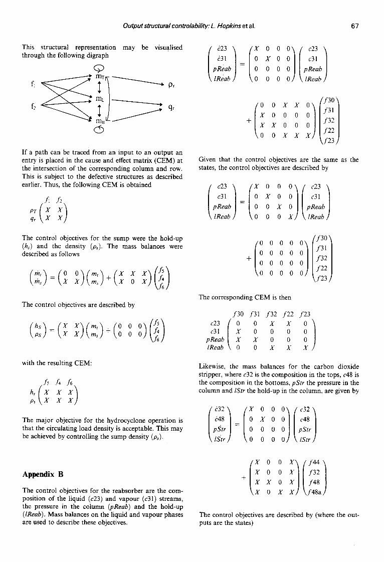
This structural representation may be visualised through the following digraph

Q

f 0r

mc/- - - - - -______ ~

f~ m ~ f q'

C~

If a path can be traced from an input to an output an entry is placed in the cause and effect matrix (CEM) at the intersection of the corresponding column and row. This is subject to the defective structures as described earlier. Thus, the following CEM is obtained

A A

The control objectives for the sump were the hold-up (hs) and the density (Ps). The mass balances were described as follows

(m;) = ( 0 1 ) ( m s ) + ( ~ 0 X ) \ f 6


(hp:) = (X m, 0 ~ ) ( ; 5 4 / s)( )+(00 0 ms \ f 6 ]

with the resulting CEM:

f5 f4 f6

p~ X X

The major objective for the hydrocyclone operation is that the circulating load density is acceptable. This may be achieved by controlling the sump density (Ps).

,23, (ioo k3l / = x o pReab I 0 0 lReab ] 0 0

~) f C23 '~ / c31 / IPR<ab I \ lReab /

+

/ f 3 0 '~ (0 0 ' x o o o / f 3 2 1 X X 0 0 1f22 ] 0 0 X X \ f 2 3 ]

Given that the control objectives are the same as the states, the control objectives are described by

c23, (i o o i/ c23, c 3 1 | = X 0 /~3'/ pReab I 0 X IPReabl lReab ] 0 0 \ lReab ]

+

°°°°i/ 0 0 0 0

0 0 0 0

0 0 0 0

' f30 '~

f31 i f 3 2 ]

f22 /

,f23 ]

The corresponding CEM is then

f30 f31 f32 f22 f23 c23 ( O O X X O ) c31 X 0 0 0 0

pReab X X 0 0 0 1Reab 0 0 X X X

Likewise, the mass balances for the carbon dioxide stripper, where c32 is the composition in the tops, c48 is the composition in the bottoms, pStr the pressure in the column and lStr the hold-up in the column, are given by

( 32, (i 0 0 !i c32 ~4s / = ~ 0 / c48 pStr I 0 0 IPStr lStr / 0 0 \ lStr

Appendix B

The control objectives for the reabsorber are the composition of the liquid (c23) and vapour (c31) streams, the pressure in the column (pReab) and the hold-up (lReab). Mass balances on the liquid and vapour phases are used to describe these objectives.

+ x ° ° i)/J ) X 0 0 f32

X X 0 | f48

X 0 X \ f 4 8 a

The control objectives are described by (where the outputs are the states)


c32,/i o o i//c32, c48 / = X 0 / c48 / pStr I 0 X IpStr I lStr / _0 0 \ lStr /

+

(i ° ° 0 0 f32

0 0 1 f 4 8 / 0 0 \ f48a /

Giving the following CEM

f44 f32 f48 f48a

c48 X 0 0 X pStr X X 0 X IStr X 0 X X

The refining column is a distillation column with reboi- ler, overhead condenser and reflux drum. The control objectives are the compositions of the tops (c44) and bottoms (c35), the column pressure (pRef), and the hold-ups in the drum (IRCR) and column (lRef). They are described by the mass balances given as follows (i0000]

c3 / ooo pR.ef |= 0 0 0 0 I pRefl ;~ f~ / o o o o / ; ~ c ~ / lRef ] 0 0 0 0 \ lRef ]

+ (i i] X O 0 X X O f44 .

0 0 X X f35

0 0 0 X 1 f 4 5 1 X 0 X 0 | f 3 6 a / 0 X X X \ f 3 9 /

The control objectives are described by: / (ioooo/c ooo

p r e y | = 0 X 0 0 [pRey I tRcR/ o o x o / ' R c R / lRef ] 0 0 0 X \ lRef,]

0 0 0 0 0 0 f44

0 0 0 0 0 f35

0 0 0 0 0 | f 4 5 1 0 0 0 0 0 [ f36a~ 0 0 0 0 0 \ f 3 9 /

Giving the following CEM

f33 f44 f35 f45 f36a f39 o / c34 X 0 0 X X 0

pRef 0 0 0 0 X X lRCR 0 X 0 X 0 X lRef X 0 X X X 0

The heat exchangers are described by energy balances, the control objectives being the temperatures of the outlet streams. For heat exchanger 4 the energy balances are

t47 J ( X = X X ) ( / 2 2 t 4 7 ) + ( X X X) ff21~\f46J


(' t22"~ = (t22 0 0 t47 J ( X 0 o) )+(00 \ t47 ) ( ' f21)

\ f 46 J

and the CEM is

f21 f46 t 2 2 ( X X ) t47 X X

Output strutural controllability: a tool for integrated process design and control

Documents

Transcript of Output strutural controllability: a tool for integrated process design and control