Outlook for Natural Gas Demand for the - · PDF file · 2016-06-01Outlook for...
42
5/26/2016 1:51 PM 1 2016 NGSA Summer Outlook Outlook for Natural Gas Demand for the Summer of 2016 Prepared by Energy Ventures Analysis, Inc. Overview Summer period gas demand is expected to increase approximately 4.1 BCFD, or 6.3 percent, with most of this increase occurring because of the combination of structural changes within the electric sector and increased coal-to-gas fuel switching (see Exhibit 1). Offsetting this increase in demand will be about a 50 percent decline in storage injections this year (i.e., 5.2 BCFD lower), which largely is due to storage levels at the beginning of the summer season (April 1, 2016) being at record levels. 1 The net result will be season ending storage levels (October 31, 2016) being at about 3,875 BCF, which, while below last year’s season ending levels, is above season ending levels for 2014. As noted in Exhibit 1, approximately 85 percent of the expected increase in summer demand (i.e., primary demand) will occur within the electric sector. This increase in electric sector demand is due to the combination of (1) structural changes within the electric industry that have occurred over the last several years and have caused reductions in coal-fired capacity and increases in gas-fired capacity; and (2) near record coal-to-gas fuel switching which is occurring because of the current low gas prices. Additive to this are relatively small increases in the industrial, residential and commercial sectors. Exhibit 1. Projected Gas Demand for April Through October 2016 (1) 2016 2015 Change Sector BCF Average BCFD BCF Average BCFD BCF Average BCFD Residential 1,196 5.6 1,148 5.4 48 0.2 Commercial 1,146 5.4 1,135 5.3 11 0.1 Industrial 4,237 19.8 4,181 19.5 56 0.3 Electric 6,761 31.6 6,089 28.5 672 3.1 Lease, Plant & Pipeline Fuel 1,454 6.8 1,368 6.4 86 0.4 Subtotal 14,794 69.2 13,921 65.1 873 4.1 Net Storage Injections 1,357 6.3 2,475 11.5 (1,118) (5.2) Source: EIA and EVA. (1) Figures may not add due to rounding. 1 For purposes of this report, summer refers to the period April through October, even though technically this period includes part of the spring and fall seasons. This terminology is used in order to simplify the discussion contained in this report.
Transcript of Outlook for Natural Gas Demand for the - · PDF file · 2016-06-01Outlook for...

5/26/2016 1:51 PM 1 2016 NGSA Summer Outlook
Outlook for Natural Gas Demand for the Summer of 2016
Prepared by Energy Ventures Analysis, Inc.
Overview Summer period gas demand is expected to increase approximately 4.1 BCFD, or 6.3
percent, with most of this increase occurring because of the combination of structural
changes within the electric sector and increased coal-to-gas fuel switching (see Exhibit
1). Offsetting this increase in demand will be about a 50 percent decline in storage
injections this year (i.e., 5.2 BCFD lower), which largely is due to storage levels at the
beginning of the summer season (April 1, 2016) being at record levels.1 The net result
will be season ending storage levels (October 31, 2016) being at about 3,875 BCF, which,
while below last year’s season ending levels, is above season ending levels for 2014.
As noted in Exhibit 1, approximately 85 percent of the expected increase in summer
demand (i.e., primary demand) will occur within the electric sector. This increase in
electric sector demand is due to the combination of (1) structural changes within the
electric industry that have occurred over the last several years and have caused reductions
in coal-fired capacity and increases in gas-fired capacity; and (2) near record coal-to-gas
fuel switching which is occurring because of the current low gas prices. Additive to this
are relatively small increases in the industrial, residential and commercial sectors.
Exhibit 1. Projected Gas Demand for April Through October 2016(1)
2016 2015 Change
Sector
BCF
Average
BCFD
BCF
Average
BCFD
BCF
Average
BCFD
Residential 1,196 5.6 1,148 5.4 48 0.2
Commercial 1,146 5.4 1,135 5.3 11 0.1
Industrial 4,237 19.8 4,181 19.5 56 0.3
Electric 6,761 31.6 6,089 28.5 672 3.1
Lease, Plant &
Pipeline Fuel
1,454 6.8 1,368 6.4 86 0.4
Subtotal 14,794 69.2 13,921 65.1 873 4.1
Net Storage Injections 1,357 6.3 2,475 11.5 (1,118) (5.2) Source: EIA and EVA. (1) Figures may not add due to rounding.
1 For purposes of this report, summer refers to the period April through October, even though technically this period
includes part of the spring and fall seasons. This terminology is used in order to simplify the discussion contained in
this report.

5/26/2016 1:51 PM 2 2016 NGSA Summer Outlook
With respect to significant risk factors for this outlook, there are two noteworthy items,
namely (1) the summer weather and (2) the potential for declining domestic production.
Concerning the former, the NOAA forecast is for a slightly warmer than normal summer
(i.e., 7.6 percent warmer than normal), which is below last year’s very warm summer
(i.e., 10.3 percent warmer than normal), but above the relatively normal summer in 2014
(i.e., 0.2 percent warmer than normal). The key concern is that if this summer turns out
to be a hot summer then electric gas demand could be higher, while a cooler summer
would lower projected electric sector demand.2
With respect to domestic production, production for nearly every onshore play is
declining because of the 75 percent decrease in gas-directed drilling activity since peak
levels in late 2014.3 However, offshore production is expected to increase as a result of
the bringing online of a series of legacy offshore projects in 2015 and 2016, which take
time to ramp up to full production (i.e., 14 projects in 2015 and 10 projects in 2016). As a
result, there is some uncertainty as to the net decline in domestic production this summer.
This, in turn, impacts the level of storage injections during the summer, with high
production levels from a lower rate of decline causing storage injections to increase and
vice-a-versa.
Exhibit 2 provides a longer term overview of historical trends for summer gas demand.
As illustrated, 2016 summer gas demand will exceed the record set last year, when a
combination of very hot weather and record fuel switching caused summer demand to
soar.
2 Cooling degree days for periods noted are as follows: 30-yr average = 1,245; 2016 = 1,339; 2015 = 1,373; 2014 =
1,247; 2013 = 1,293; 2012 = 1,382; 2011 = 1,340; 2010 = 1,430; and 2009 = 1,174. 3 The gas-directed rig count in early November 2014 was 356 rigs, while the current rig count is 88 rigs. In April
2015 (i.e., one year ago) the gas-directed rig count was 217.

5/26/2016 1:51 PM 3 2016 NGSA Summer Outlook
Exhibit 2. Summer Natural Gas Demand for All Sectors
53.1 54.7 53.7 53.3 55.9 57.6
63.0 60.5 61.2
65.1 69.2
0.0
10.0
20.0
30.0
40.0
50.0
60.0
70.0
80.0
2006 2007 2008 2009 2010 2011 2012 2013 2014 2015 2016
(BCFD)Summer Natural Gas Demand for All Sectors
Normal Summer Hot Summer
Note: 2016 natural gas demand is forecasted.2006, 2007, 2010, 2011, 2012, 2015, and 2016 denote hot summers.
Outlook for Demand
Overview
The following discussion provides an assessment of summer demand for each of the four
major sectors. The impact of storage injections is addressed in a subsequent section.
Residential and Commercial
Residential and commercial sector gas demand for the forthcoming summer is, in
essence, expected to be slightly higher than the prior summer’s demand levels, which
happen to represent a low point for the last three summers. These two winter weather-
sensitive sectors usually are not affected significantly by changes in the summer weather.
Finally, Exhibit 3 summarizes the longer term trends for summer gas demand within both
sectors.

5/26/2016 1:51 PM 4 2016 NGSA Summer Outlook
Exhibit 3. Summer Natural Gas Demand for the Residential and Commercial Sectors
6.0 6.2 6.2 5.5 5.9 5.3 5.9 5.8 5.4 5.6 5.1 5.3 5.3 5.0 5.4 5.2 5.5 5.6 5.3 5.4 0.0
1.0
2.0
3.0
4.0
5.0
6.0
7.0
2007 2008 2009 2010 2011 2012 2013 2014 2015 2016 2007 2008 2009 2010 2011 2012 2013 2014 2015 2016
(BCFD)
Residential Commercial
Note: 2016 residential and commercial sector natural gas demand is forecasted.Source: EIA and EVA
Industrial Sector
The change in industrial sector gas demand for this summer is complex, as industrial
demand for existing industrial facilities is declining; however, this decline is being offset
by a series of capacity expansions in a few key industries. The net result is an expected
1.3 percent, or 0.3 BCFD, increase over last summer’s results.
Capacity Expansions With respect to the series of capacity expansions occurring within the industrial sector,
which are being built to take advantage of the relatively low cost gas in the U.S. The
2016 to 2018 period will mark the peak period for the annual additions of these projects.
This is illustrated in Exhibit 4. For the most part these projects are expanding capacity in
selected industries, in order to use relatively inexpensive U.S. natural gas to produce
products (e.g., petrochemical and fertilizer) that either increase U.S. exports or
alternatively reduce U.S. imports.

5/26/2016 1:51 PM 5 2016 NGSA Summer Outlook
Exhibit 4. Industrial Capacity Expansion Projects(1),(2)
While there have been some additions and deletions to the list of industrial capacity
expansion projects, at present there are 106 likely capacity addition projects in the
fertilizer, petrochemical, methanol, steel and paper and pulp industries. Of these 106
projects 38 came online in the 2010 to 2014 period and an additional seven came online
in 2015. The remaining 61 projects are projected to come online in the 2016 to 2020
timeframe.
With respect to 2016, this year will receive the benefit of the full year impact of the seven
projects that came online in 2015, plus the partial year impact of 15 additional projects
scheduled to come online in 2016. The net result is that summer gas demand within the
industrial sector is expected to increase approximately 0.65 BCFD, as a result of just
these capacity expansion projects coming online.
Existing Facilities While there has been modest growth in the U.S. economy (see Exhibit 5), this growth has
not been even across all sectors of the economy. More specifically, for most of the last
seven months there has been a decline within the manufacturing sector of the economy.
This decline is occurring within every industry except automobiles and is particularly
acute within the oil field services and mining sector, which is down sharply. Other factors
adversely impacting the manufacturing sector are (1) the limited growth prospects for the
global economy and (2) the relatively strong U.S. dollar.

5/26/2016 1:51 PM 6 2016 NGSA Summer Outlook
Exhibit 5. U.S. Real GDP Short-Term Forecast Comparison
14,000
14,750
15,500
16,250
17,000
17,750
18,500
Q1
-20
08
Q2
-20
08
Q3
-20
08
Q4
-20
08
Q1
-20
09
Q2
-20
09
Q3
-20
09
Q4
-20
09
Q1
-20
10
Q2
-20
10
Q3
-20
10
Q4
-20
10
Q1
-20
11
Q2
-20
11
Q3
-20
11
Q4
-20
11
Q1
-20
12
Q2
-20
12
Q3
-20
12
Q4
-20
12
Q1
-20
13
Q2
-20
13
Q3
-20
13
Q4
-20
13
Q1
-20
14
Q2
-20
14
Q3
-20
14
Q4
-20
14
Q1
-20
15
Q2
-20
15
Q3
-20
15
Q4
-20
15
Q1
-20
16
Q2
-20
16
Q3
-20
16
Q4
-20
16
Q1
-20
17
Q2
-20
17
Q3
-20
17
Q4
-20
17
Q1
-20
18
Q2
-20
18
Q3
-20
18
Q4
-20
18
(Billion $2009)
U.S. Real GDP Short-Term Forecast Comparison
WSJ Range
WSJ Mean
Moody's
BEA Actuals
AEO 2015
Exhibit 6 summarizes the production indices for the six major energy intensive industries.
While there are month to month variations in these indices, three of the six industries,
namely non-metallic, paper and primary metals, are exhibiting downward trends for their
production indices. In addition, two of these energy intensive industries, namely food and
chemicals, recently have had relatively flat indices. With respect to the sixth index,
namely petroleum and coal, lately it has shown some signs of recovery after an earlier
decline. The net result of this assessment is that gas demand for existing industrial
facilities is expected to decline this summer by about 0.35 BCFD, or 1.5 percent.
Summary With respect to the integrated outlook for industrial sector gas demand this summer, it is
expected to increase 0.3 BCFD, or 1.3 percent, over last year’s level. As an added point
of perspective, Exhibit 7 compares and contrasts, on an annual basis, the expected
outlook for 2016 industrial sector gas demand with the consumption levels for the sector
since 2000. As illustrated, during the prior decade the dominant trend for industrial
sector gas demand was decline, as the sector initially experienced significant price
elasticity during the era of high gas prices that occurred during the first half of the
decade. This was compounded by the impact of the Great Recession during the second
half of the decade. However, currently with the ratio of oil-to-gas prices at about 21:1
U.S. industrial gas demand is not nearly as sensitive to changes in gas prices as in the
past, when the ratio of oil-to-gas prices was closer to 6:1.

5/26/2016 1:51 PM 7 2016 NGSA Summer Outlook
Exhibit 6. Performance of the Six-Key Energy Intensive Industries
98
100
102
104
106
Jan
-12
Mar
-12
May
-12
Jul-
12
Sep
-12
No
v-1
2
Jan
-13
Mar
-13
May
-13
Jul-
13
Sep
-13
No
v-1
3
Jan
-14
Mar
-14
May
-14
Jul-
14
Sep
-14
No
v-1
4
Jan
-15
Mar
-15
May
-15
Jul-
15
Sep
-15
No
v-1
5
Jan
-16
Mar
-16
Index 2007=100
Food (311)
94
96
98
100
102
104
106
Jan
-12
Mar
-12
May
-12
Jul-
12
Sep
-12
No
v-1
2
Jan
-13
Mar
-13
May
-13
Jul-
13
Sep
-13
No
v-1
3
Jan
-14
Mar
-14
May
-14
Jul-
14
Sep
-14
No
v-1
4
Jan
-15
Mar
-15
May
-15
Jul-
15
Sep
-15
No
v-1
5
Jan
-16
Mar
-16
Index 2007=100
Chemicals (325)
96
100
104
108
112
116
120
Jan
-12
Mar
-12
May
-12
Jul-
12
Sep
-12
No
v-1
2
Jan
-13
Mar
-13
May
-13
Jul-
13
Sep
-13
No
v-1
3
Jan
-14
Mar
-14
May
-14
Jul-
14
Sep
-14
No
v-1
4
Jan
-15
Mar
-15
May
-15
Jul-
15
Sep
-15
No
v-1
5
Jan
-16
Mar
-16
Index 2007=100
NonMetallic (327)
95
97
99
101
103
Jan
-12
Mar
-12
May
-12
Jul-
12
Sep
-12
No
v-1
2
Jan
-13
Mar
-13
May
-13
Jul-
13
Sep
-13
No
v-1
3
Jan
-14
Mar
-14
May
-14
Jul-
14
Sep
-14
No
v-1
4
Jan
-15
Mar
-15
May
-15
Jul-
15
Sep
-15
No
v-1
5
Jan
-16
Mar
-16
Index 2007=100
Paper (322)
98
100
102
104
106
108
110
Jan
-12
Mar
-12
May
-12
Jul-
12
Sep
-12
No
v-1
2
Jan
-13
Mar
-13
May
-13
Jul-
13
Sep
-13
No
v-1
3
Jan
-14
Mar
-14
May
-14
Jul-
14
Sep
-14
No
v-1
4
Jan
-15
Mar
-15
May
-15
Jul-
15
Sep
-15
No
v-1
5
Jan
-16
Mar
-16
Index 2007=100
Petroleum & Coal (324)
90
93
96
99
102
105
108
Jan
-12
Mar
-12
May
-12
Jul-
12
Sep
-12
No
v-1
2
Jan
-13
Mar
-13
May
-13
Jul-
13
Sep
-13
No
v-1
3
Jan
-14
Mar
-14
May
-14
Jul-
14
Sep
-14
No
v-1
4
Jan
-15
Mar
-15
May
-15
Jul-
15
Sep
-15
No
v-1
5
Jan
-16
Mar
-16
Index 2007=100
Primary Metals (331)
Source: Federal Reserve.

5/26/2016 1:51 PM 8 2016 NGSA Summer Outlook
Exhibit 7. Summer Natural Gas Demand for the Industrial and Transportation Sectors
2000
21.2
21.2
19.2
19.9
18.6 18.9
17.1 17.2 17.2 17.3
15.9
17.7
18.2
19.1 19.3
19.8 19.5
19.8
14.0
16.0
18.0
20.0
22.0
2000 2001 2002 2003 2004 2005 2006 2007 2008 2009 2010 2011 2012 2013 2014 2015 2016
(BCFD)
Source: EIA and EVA.
Actual Forecasted
Price Elasticity
Great Recession
Starting in 2010, however, this basic downward trend for industrial sector gas demand
reversed itself, as the country began to emerge from the Great Recession and the sector
benefitted from the initial impact of the previously noted series of capacity additions.
Electric Sector
The primary factors driving the 11 percent, or 3.1 BCFD, increase in electric sector
summer demand are (1) the structural changes that have occurred within the industry over
the last several years and (2) the increase in coal-to-gas fuel switching because of the
current relatively low gas prices.4 The major uncertainty factor for this assessment is the
peak summer weather (i.e., July and August), as the difference in electric sector gas burn
between a mild and very hot summer can be approximately 300 BCF (i.e., equivalent to
1.4 BCFD) over the summer period.
Exhibit 8 summarizes summer gas demand for the electric sector over the last 10 years
and highlights both the impact of very warm summer weather and coal-to-gas fuel
switching.
4 Another factor that has, in the past, influenced summer electric sector gas burn has been changes in hydroelectric
generation for California and the Northwest, as gas-fired generation is the primary alternative to hydroelectric
generation. While the influence of this factor has been significant over the last couple of years, because of the
drought conditions in California, that will not be the case for 2016.

5/26/2016 1:51 PM 9 2016 NGSA Summer Outlook
Exhibit 8. Summer Natural Gas Demand for the Electric Sector
15.7 16.8
18.6 20.2
22.6 22.9
27.9
23.9 24.0
28.5
31.6
0.0
5.0
10.0
15.0
20.0
25.0
30.0
35.0
2006 2007 2008 2009 2010 2011 2012 2013 2014 2015 2016
(BCFD)
Actual Hot Summer Coal-to-Gas Fuel Switching
Note: 2006, 2007, 2010-2012, and 2015-2016 denote hot summers.Demand and coal-to-gas fuel switching for 2016 is forecasted.
Structural Changes Over the last several years coal-fired capacity has been declining, while gas-fired
capacity has been increasing, with the net result being increased market share for gas-
fired generation. Exhibit 9 provides specifics for this phenomenon over the last five
years. As illustrated, on a net basis, coal-fired capacity has declined about 38.2 GW over
the last five years, while combined cycle (CCGT) gas-fired capacity has increased about
27.3 GW, with most of this transition occurring within the last two years. Going forward
it is anticipated this trend will accelerate, as during 2016 and 2017 another 19.2 GW of
coal-fired capacity is expected to retire, while new build CCGT units will total about 19.4
GW.
For summer gas demand the net effect of this structural change within the electric
industry is an estimated increase in electric sector gas consumption of approximately 2.2
BCFD (i.e., about 70 percent of the overall increase in electric sector gas consumption).

5/26/2016 1:51 PM 10 2016 NGSA Summer Outlook
Exhibit 9. New U.S. Generation Capacity
(MW) 2011 2012 2013 2014 2015 2016 2017Coal-Fired 2,665 3,760 1,507 580 - - -
Solar 534 1,702 2,959 1,724 2,231 3,851 2,629
Wind(1) 6,800 12,885 1,032 2,028 7,099 3,898 6,052 Gas Combined Cycle 7,259 6,713 3,511 6,383 3,384 7,145 12,289
Gas Peaking 1,752 2,334 3,332 250 1,212 2,175 1,716 Total Gas-Fired 9,011 9,047 6,842 6,633 4,596 9,320 14,005 Grand Total 19,010 27,394 12,340 10,965 13,926 17,069 22,685
Retirements (Coal) 3,280 10,891 6,951 5,568 20,049 12,565 6,657
Retirements (Nuclear)(2)
- - 2,716 563 - - 1,496 (1) Wind capacity for 2016 and 2017 estimated, as proposed projects significantly exceed these estimates.
(2) EVA assumes that the James A Fitspatrick and R E Ginna nuclear plants will shut down in 2017.
Projected
Fuel Switching Coal-to-gas fuel switching during this summer is estimated to be about 0.9 BCFD greater
than last summer’s fuel switching. This is occurring because of the anticipated lower gas
prices this summer versus the last summer (i.e., $2.29 versus $2.68 per MMBTU). As a
point of perspective, fuel switching for this summer is expected to be only second to the
levels attained in 2012, when fuel switching capacity was much higher (i.e., about 10
percent less).
Exhibit 10 provides a summary of monthly fuel switching over approximately the last
three years in billion cubic feet per day (BCFD) of natural gas demand. Highlighted in
Exhibit 10, by the red portions of the bars, is the amount of prior fuel switching that has
been converted to permanent gas-fired generation because of the retirement of coal-fired
units. The blue bars indicate the amount of fuel switching that still remains and is a
function of the relative regional prices of coal and gas-fired generation.5
5 These generation data convert to the following natural gas outcomes, all in BCFD: 2012 permanently displaced
(PD) 0.8, coal switching (CS) 5.3, total 6.1; 2013 PD 1.3, CS 3.5 total 4.8; 2014 PD 2.0, CS 3.0, total 4.9; 2015 PD
3.4, CS 4.7, total 8.1.

5/26/2016 1:51 PM 11 2016 NGSA Summer Outlook
Exhibit 10. Coal-to-Gas Fuel Switching
Permanently Displaced Coal Generation - (TWh)
Jan-13
3.60
0.00
3.61
Coal Switching (TWh)
$0.00
$1.50
$3.00
$4.50
$6.00
$7.50
-
2.0
4.0
6.0
8.0
10.0
12.0
Jan
-13
Feb
-13
Mar
-13
Ap
r-1
3M
ay-1
3Ju
n-1
3Ju
l-1
3A
ug-
13
Sep
-13
Oct
-13
No
v-1
3D
ec-
13
Jan
-14
Feb
-14
Mar
-14
Ap
r-1
4M
ay-1
4Ju
n-1
4Ju
l-1
4A
ug-
14
Sep
-14
Oct
-14
No
v-1
4D
ec-
14
Jan
-15
Feb
-15
Mar
-15
Ap
r-1
5M
ay-1
5Ju
n-1
5Ju
l-1
5A
ug-
15
Sep
-15
Oct
-15
No
v-1
5D
ec-
15
Jan
-16
Feb
-16
Mar
-16
Coal Switching
Permanently Displaced CoalGeneration
Henry Hub Price
Gas Price $/MMBTU(BCFD)
Electric Sales Among the other factors that historically have influenced electric sector gas demand is
the overall growth in electricity sales. During periods of significant sales growth, this can
be a significant factor in determining overall electric sector gas demand, because gas-
fired generation tends to be at the margin in most regions. Exhibit 11 summarizes the
year-to-date growth in electricity sales. As illustrated, on a year-to-date basis electricity
sales figures for 2016 are below those for 2015. This year-to-date comparison primarily is
due to the warm winter this year. For the summer it is anticipated that electricity sales
will be flat to slightly below last year’s results. The net result is that changes in
electricity sales this summer are expected to have a rather limited impact on electric
sector gas demand.

5/26/2016 1:51 PM 12 2016 NGSA Summer Outlook
Exhibit 11. Total Weekly Electric Output (48-States)
60,000
65,000
70,000
75,000
80,000
85,000
90,000
95,000
100,000
1 4 7 10 13 16 19 22 25 28 31 34 37 40 43 46 49 52
(GWH)
Source:EEI.
Total Weekly Electric Output (48 States)
2014 2015 2016
(Week of the Year)
Summer Weather With respect to the influence of summer weather, Exhibit 12 compares and contrasts peak
month electric sector gas demand for each of the last seven years with the outlook for the
peak month in 2016. Also, included in this graphic is the CDD for each month. The data
in this exhibit presents the lowest to highest peak demand levels for the selected years.
While there is not a perfect correlation between peak electric gas consumption levels and
CDD,6 the general trend is readily apparent. With July 2016 it is impacted by structural
changes within the industry, as well as warm summer weather.
6 In addition to differences in the warmth of the summer weather, gas-fired generation in a specific month can be
affected by a number of factors (e.g., unplanned outages of nuclear and coal units, availability of renewable
capacity, etc.).

5/26/2016 1:51 PM 13 2016 NGSA Summer Outlook
Exhibit 12. Comparison of Summer Peak Period Natural Gas Demand for the Electric Sector and Cooling Degree Days
27.129.0 29.4
30.3 30.4
34.0 34.9
38.3
100
200
300
400
500
0.0
5.0
10.0
15.0
20.0
25.0
30.0
35.0
40.0
Aug-09 Aug-14 Jul-13 Jul-11 Aug-10 Jul-15 Jul-12 Jul-16
(BCFD)
Actual Coal-to-Gas Fuel Switching Cooling Degree Days
Note: 2016 demand, fuel switching, and cooling degree days for are forecasted.Source: EIA and NOAA.
(CDD)
Storage Injections Probably the most difficult element to project in this assessment of 2016 summer gas
demand is the final component of the demand picture, namely 2016 storage injections.
The current outlook for storage injections for this summer is that they will be relatively
low, primarily because storage levels at the end of the winter season (March 31, 2016)
were at record levels. As a result, injections do not need to be high in order to have
adequate storage levels at the beginning of the next winter. The primary factor in
ensuring the storage injections are at relatively low levels is increased levels of coal-to-
gas fuel switching, and fuel switching in 2016 is expected to be the second highest level
ever recorded.
Exhibit 13 compares and contrast storage injections for this summer with those over the
last 10 years. As illustrated, storage injections, while below the last two years, are likely
to be on a par with injections for 2012, when storage levels at end of the winter season
also were at record levels. The net results that season ending storage levels for 2016
(October 31, 2016) are expected to be about 3,875 BCF, which is below 2015 levels but
above 2014 levels.

5/26/2016 1:51 PM 14 2016 NGSA Summer Outlook
Exhibit 13. U.S. Storage Injections
8.3
9.4
10.4 10.2 10.3 10.4
7.1
9.9
12.9
11.6
6.3
0.0
2.0
4.0
6.0
8.0
10.0
12.0
14.0
2006 2007 2008 2009 2010 2011 2012 2013 2014 2015 2016
U.S. Storage Injections(BCFD)
Note: 2016 is estimated.Source: EIA.
There are two factors that could alter this assessment – potentially significantly – namely
the summer weather and the current decline in onshore production – both of which are
discussed below. Additionally, a brief review of the impact of the timely, but primarily
regionally-significant closure of the Aliso Canyon storage facility in Southern California
is provided.
Summer Weather: While the summer weather is projected to be about 7.6
percent warmer than normal, the summers of 2011, 2012 and 2015 were greater
than 10 percent warmer than normal. If the latter where to occur in 2016, then
electric sector burn could be 150 to 200 BCF higher, with storage levels being
lower. There likely is not a perfect correlation between these two elements, as fuel
switching during later part of summer likely would decline. Nevertheless, the net
result likely would be lower storage levels at the end of the summer season.
Conversely, if this summer’s weather turns out to be relatively mild, like the
summers of 2008 and 2009, storage levels would be higher.
Domestic Production: At present nearly every onshore gas play is declining,
because of the overall decline in drilling activity (i.e., see Exhibit 14, which
summarizes the 75 percent decline in the gas-directed rig count). Offsetting this
decline in onshore production is the anticipated increase in offshore production, as
a result of the ramping up of production for a series of legacy offshore projects
(i.e., 14 projects in 2015 and 10 projects in 2016).

5/26/2016 1:51 PM 15 2016 NGSA Summer Outlook
Exhibit 14. Rig Count for Gas Wells
$0
$1
$2
$3
$4
$5
$6
$7
$8
$9
$10
$11
0
100
200
300
400
500
600
700
800
900
2012 2013 2014 2015 2016
($/MMBTU)No. of Gas Rigs
No. of Rigs Henry Hub Price
Note: Blue bars represent the number of gas rigs on even years while gray bars represent odd years.Source: NGW.
If the overall decline in domestic production is less than anticipated, then season
ending storage levels could be higher. However, if the opposite occurs, they could
be lower.
Lastly, Exhibit 15 compares and contrasts season ending storage levels for the last several
years with that expected for October 31, 2016.
Exhibit 15. Comparison of Storage Capacity and Season-Ending (November 1) Storage Levels
Est.
2007 2008 2009 2010 2011 2012 2013 2014 2015 2016
Total Working Gas Capacity - Start of Injection Season(1) 3,593 3,665 3,754 3,925 4,049 4,103 4,265 4,333 4,336 4,343
Annual Capacity Additions 72 89 171 124 54 162 68 3 7 -
Total Working Gas Capacity - End of Injection Season 3,665 3,754 3,925 4,049 4,103 4,265 4,333 4,336 4,343 4,343
Storage Level at Start of Winter 3,567 3,399 3,810 3,847 3,804 3,929 3,817 3,587 3,953 3,875
Percent of Capacity 97% 91% 97% 95% 93% 93% 88% 83% 91% 89%
1. Effective maximum usable working capacity.
Actual
Aliso Canyon: In October 2015, a leak was discovered at an injection well within
Southern California Gas Company’s (SoCal) largest storage field and would
become the largest singular methane leak in U.S. history. As a result, the 86.2 Bcf
of working-gas storage capacity7 at Aliso Canyon is non-operational and
7 Aliso Canyon’s 86.2 Bcf is the largest storage facility in California, with 22.9% of the state’s capacity and 63.7%
of Southern California’s 135.3 Bcf of capacity. However, it represents only 1.9% of total lower-48 capacity.

5/26/2016 1:51 PM 16 2016 NGSA Summer Outlook
unavailable to the Southern California natural gas markets until further notice.
This presents an operational challenge for the region’s gas markets as the removal
of Aliso Canyon impacts the ability for the Southern California gas market to
absorb daily imbalances. However, the region’s wide array of gas infrastructure,
including 1.82 BCFD of working storage withdrawal capacity at SoCal’s three
remaining storage fields8 and over 4 BCFD of regional import capacity with large
interstate pipelines9 present powerful tools to manage SoCal’s average and peak
summer demand of 2.5 and 3.6 BCFD, respectively. The ultimate impact of this
event will be greatly determined by the summer weather Southern California
receives.
Exports While technically part of the supply components for natural gas, exports of natural gas
does represent another draw on domestic production. As a result, recent events
concerning the 2016 exports are reviewed briefly in the following material.
LNG Exports
In late February the first export of L-48 LNG occurred from Train 1 of Cheniere’s Sabine
Pass liquefaction facilities. This shipment is part of eight commissioning cargoes (i.e.,
about 32 BCF) for Train 1, with the first seven cargoes already having occurred.10 These
initial exports represent spot cargoes into a very competitive global market. Contracted
cargoes using Sabine Pass tolling contract approach are scheduled to begin in November,
which is when Sabine Pass’ contract with Shell/BG begins. While these initial shipments
likely will result in only 0.5 BCFD of LNG exports for the summer of 2016, by year-end
2018 L-48 LNG exports are projected to reach about 3.8 BCFD, as eight additional trains
from various projects are projected to come online.
Exports To Mexico
Exports to Mexico have been increasing steadily over the last five years and are expected
to also increase in 2016. With respect specifically to the summer of 2016, exports to
Mexico are projected to increase approximately 0.95 BCFD.
The primary factor behind this steady increase in exports to Mexico is the building of
new pipeline capacity on both sides of the border and, in particular, on the Mexican side
of the border, which historically has been the limiting factor for exports to Mexico.
8 Honor Rancho and Playa del Ray in Los Angeles County and La Goleta in Santa Barbara County. 9 Pipelines include El Paso Natural Gas, Transwestern, Kern River Gas Transmission, Mojave Pipeline and Southern
Trails Pipeline 10 The first seven cargoes were sent to various destinations, including Brazil (twice), Argentina, Portugal, India and
Dubai.

5/26/2016 1:51 PM 17 2016 NGSA Summer Outlook
Addendum I of this report provides a detailed assessment of these pipeline projects and
the longer term expectations for exports to Mexico.
Ethane
While technically not part of the natural gas supply and demand, ethane is a key
component of raw gas volumes at the wellhead. Recently, the U.S. initiated its first
exports of ethane, which represents a significant milestone in that the U.S. currently has
significant excess supplies of ethane, as a result of the surge in unconventional drilling
for the shale plays.
More specifically, on March 9th the first U.S. shipment of ethane left the Marcus Hook
terminal near Philadelphia. This ethane shipment, which is part of a 15-year contract
between Range Resources and Ineos went to the Ineos petrochemical in Rafnes, Norway.
The ethane was delivered to Sunoco’s Marcus Hook terminal via the recently completed
Mariner East 1 pipeline, which originates near Pittsburgh. An expansion of this pipeline,
namely the Marine East 2 pipeline, is under construction. Finally, a second ethane export
terminal at Morgan’s Point, Texas is scheduled to be completed by Enterprise Product
Partners in the 3Q 2016.
Conclusions As illustrated in Exhibit 16 summer gas demand this year should be approximately 4.1
BCFD, or 6.3 percent, greater than demand last summer. Furthermore, gas demand this
summer will set a new record, as it will exceed the prior records set in 2012 and 2015.
Approximately 85 percent of projected increase in summer demand (i.e., primary
demand) will occur within the electric sector, as a result of both (1) recent structural
changes within the industry and (2) increased levels of fuel switching.
Offsetting this increase in demand will be about a 50 percent decline in storage injections
this year. However, since storage levels at the start of the summer season (April 1, 2016)
were at record levels, season ending (October 31, 2016) storage levels should be adequate
to meet storage withdrawal requirements this winter.

5/26/2016 1:51 PM 18 2016 NGSA Summer Outlook
Exhibit 16. Summer Natural Gas Demand for All Sectors
53.1 54.7 53.7 53.3 55.9 57.6
63.0 60.5 61.2
65.1 69.2
0.0
10.0
20.0
30.0
40.0
50.0
60.0
70.0
80.0
2006 2007 2008 2009 2010 2011 2012 2013 2014 2015 2016
(BCFD)Summer Natural Gas Demand for All Sectors
Normal Summer Hot Summer
Note: 2016 natural gas demand is forecasted.2006, 2007, 2010, 2011, 2012, 2015, and 2016 denote hot summers.

5/26/2016 1:51 PM 1 2016 NGSA Summer Outlook
ADDENDUM I:
OUTLOOK FOR U.S. NATURAL GAS EXPORTS TO
MEXICO

5/26/2016 1:51 PM 1 2016 NGSA Summer Outlook
Overview for U.S. Gas Exports to Mexico
Overview Cheap U.S. natural gas is driving a natural gas renaissance in Mexico. Mexican regulators
have made significant strides to continue to grow the import capacity of natural gas to
Mexico to allow both its power sector and its industrial sector to enjoy the benefits of
cheap U.S. natural gas. It is forecasted as illustrated in Exhibit Add I-1, that the Mexican
pipeline imports from the U.S. will double between 2015 and 2020.
Two key drivers behind this renaissance have been (1) the U.S. shale gas revolution and
the resulting low natural gas prices, and (2) the 2013 Mexican Energy Reform which
opened up investment opportunities for private companies. Private companies will
continue to push Mexico away from fuel-oil in power generation, which has been
Mexico's leading fuel source, and towards cheaper and greener natural gas.
This has led to the development of a series of pipeline projects both within Mexico, and
on the U.S. side. There are currently 13 pipeline projects being developed to supply U.S.
natural gas to Mexico and another 15 pipeline projects being developed in Mexico to
more efficiently transport this natural gas. There is about 5 BCFD of direct export
capacity currently being developed and scheduled to be operational before 2018. By 2019
Mexico will have the capacity to import 9 BCFD. EVA expects that this high level of
investment and continued expansion will double exports by 2020, up from 3 BCFD to 6
BCFD
Exhibit Add I-1. Mexico Natural Gas Supply
0
2
4
6
8
10
12
2011 2014 2017 2020
(BCFD)
LNG Production Mexican Net Pipeline Imports
EXHIBIT 1: MEXICO NATURAL GAS SUPPLY
5/26/2016 1:51 PM 2 2016 NGSA Summer Outlook
Mexico’s Growing Gas Demand Mexico's need for imported energy has never been greater. As can be observed in Exhibit
Add 1-2, the major source of new natural gas demand will come from the power sector.
The Mexican power sector's natural gas demand is projected to grow by 0.8 BCFD
between 2015 and 2020, a third of the projected demand growth in Mexico during that
time. CFE, the governmental electricity commission, is the major producer of electricity,
as well as transporter and retailer in Mexico. Historically, the CFE has used fuel oil as a
feedstock for power generation. However, in recent years the CFE has started a
diversification program and will switch its fleet to natural gas in the coming years. An
increased private participation in the power sector also has led to an increase in natural
gas powered combined-cycle turbines and a move away from fuel oil.
Exhibit Add I-2. Mexico Natural Gas Demand
0
2
4
6
8
10
12
2011 2014 2017 2020
(BCFD)
Residential Commercial Industrial Power Pemex
EXHIBIT 2: MEXICO NATURAL GAS DEMAND
Mexican electricity prices already have seen a decrease in recent years as a result of the
switch from fuel oil to natural gas and the increasing imports of cheap U.S. natural gas,
as can be observed in Exhibit Add I-3. Prices may not track this trend in the future as the
Mexican government may end its generous electricity rate subsidies. However, it is likely
that power prices will continue to drop as more U.S. natural gas becomes available, more
generators enter the market, and more generators switch to gas.
Another major reason for Mexico's increased natural gas imports is the on-going
manufacturing boom in Mexico. The industrial sector represents ~20% (0.45 BCFD) of
the expected growth in Mexico's natural gas demand 2015-2020. The Dollar-Peso
exchange rates have meant that producing goods in Mexico is very attractive, and more

5/26/2016 1:51 PM 3 2016 NGSA Summer Outlook
and more companies are choosing to locate their factories south of the U.S. Mexico
border. The center of this growth is located in the north central part of Mexico, in an area
called the Bajío, which has become the country's industrial heartland. A significant
amount of the existing and proposed pipelines now lead to this area, which incorporates
the states of Guanajuato, Querétaro, Aguascalientes and Jalisco. As a result the
manufacturing sectors, as well as the steel and chemical sectors, are demanding more and
more natural gas.
Exhibit Add I-3. Mexico Natural Gas Supply
0
2
4
6
8
10
12
2011
2012
2013
2014
2015
2016
2017
2018
2019
2020
(BCFD)
Source: BP Statistical Review, SENER, EVA.
Production Mexican Net Pipeline Imports LNG
EXHIBIT 5: INCREASE IN NATURAL GAS IMPORTS BY MEXICO
Production
Net Imports
LNG
Another large source of natural gas demand comes from Mexico's continued reliance on
natural gas as a feedstock for Enhanced Oil Recovery (EOR). As several large scale
projects come online in the coming years, Mexico's use of natural gas as a feedstock for
EOR will continue to increase, before plateauing around 2020. In the coming five years
Mexico likely will increase natural gas demand for EOR by 1.3 BCFD, which is a
majority of the increase during that time.
Mexico’s Stagnant Domestic Production Mexican gas production has been decreasing slightly since 2012 but is for the most part
stagnant. PEMEX has invested in natural gas production in recent years, and these
investments, as well as a growing share of gas in the oil stream, have offset the natural
decline and also somewhat increased production. However the current and future
production levels are nowhere near sufficient to keep up with the growing demand.
PEMEX has neglected to invest in natural gas production for years. This primarily is due
to poor management and political influence which geared much of the CAPEX budget
towards EOR, which is a low risk high short-term reward investment. This affected
natural gas not only because it limited the investments in production, but also because the
natural gas was and is used heavily in EOR. At the current market price, influenced by

5/26/2016 1:51 PM 4 2016 NGSA Summer Outlook
U.S. imports, it is likely that much of the natural gas reserves in Mexico will be left in the
ground for years or even decades.
Mexico has 17 TCF of proven natural gas reserves, and could in the future produce
heavily from both conventional and unconventional sources. The southern Texas shale
basins extend far into the northern border areas of Mexico. The Mexican Burgos region
alone contains 393 TCF of technically recoverable gas. Here, the keyword is ‘technically
recoverable’, because at the current level of insecurity in the area, with the current natural
gas prices and with lack of access to large volumes of water, there are very few
companies that would be willing to invest. It also would take time to build up a large
enough supporting take-away infrastructure to transport a sufficient amount of water to
this arid desert region.
Mexican LNG imports are forecasted to stop by 2020. Previously, LNG imports were
seen as the new source of natural gas for Mexico for the same reason the U.S. was
investing in LNG import terminals just five years ago. However, the shale gas revolution
changed that and LNG imports can no longer compete economically with pipeline
imports. Mexican LNG imports surged in 2013 due to pipeline constraints. Mexico
currently has two operational LNG import terminals, Altamira and Manzanillo. The 2014
utilization rate for these terminals was 40%,. This is expected to be reduced drastically in
2015 and beyond. Mexico also has a third LNG import terminal, Energia Costa Azul, that
has been considered as an export terminal. This facility is currently not receiving gas.
In order to fuel the growing exports a significant amount of natural gas pipeline capacity
has been built and will be built in the coming years. Interest from both sides of the border
has been strong, as indicated by the large investments by companies, such as Kinder
Morgan, Oneok, Energy Transfer Partners, etc. Key to allowing these companies to invest
though has been the reform which allows private sector participation in the natural gas.
This solves a key concern for the Mexican government, namely funding. At least $10 B
currently is being invested in the expansion of the pipeline system.11
The most notable change in infrastructure in recent years occurred in December of 2014
with the opening of the NET Midstream's Net Mexico pipeline. This pipeline, which has
a capacity of 2.1 BCFD, has been ramping up its capacity factor from a first full month in
January 2015, when it ran at 24% capacity factor, to October 2015, when it ran at a 48%
capacity factor.
As can be observed from Exhibit Add I-4 below, most of the U.S. sourced gas will come
from Texas, and specifically the Eagle Ford and Permian basins in South and West
Texas.
11 Based on available data. The estimated cost for all current pipelines could be twice that cost.

5/26/2016 1:51 PM 5 2016 NGSA Summer Outlook
Exhibit Add I-4. Existing Major Mexican Pipeline Infrastructure

5/26/2016 1:51 PM 6 2016 NGSA Summer Outlook
Texas Crossing There are currently 12 projects being developed to transport gas from the U.S. directly to
a destination in Mexico or to a border crossing. The most significant additions to the
export capacity of the U.S. will happen around the Clint crossing, south east of El Paso
and Ciudad Juarez, where the Samalayuca pipeline is being expanded. The Clint crossing
used to be the single largest border crossing in terms of volume until it was overtaken by
Kinder Morgan's Texas Pipeline in Roma, TX and most recently by NET Midstream’s
NET Mexico pipeline in Rio Grande. The total supporting pipelines and additions to the
Samalayuca pipeline on the U.S. side of the border have a capacity to transport 4 BCFD.
Exhibit Add I-5. Planned U.S.-Mexican Pipeline Infrastructure
Component From To Online Contractor
Roadrunner Gas Transmission (Phase I) San Elizario, TX 0.17 200 Mar-16 Oneok/Fermaca
Waha-San Elizario Waha, TX Chihuahua, MX 1.14 200 Jan-17 ETP/Carso/Mastec
San Elizario Crossing Waha Hub, TX San Elizario, TX 1.10 195 Jan-17 Energy Transfer
Roadrunner Gas Transmission (Phase II) Coyanosa, TX San Elizario, TX 0.40 Mar-17 Oneok/Fermaca
Waha-Presidio Waha, TX Ojinaga-El Encino, MX 1.35 Mar-17 Carso/Energy Transfer/MasTec
Trans-Peco Pipeline Stockton, TX Presidio, TX 1.40 Mar-17 Energy Transfer
San Isidro - Samalayuca Permian Basin, TX Norte III Plant, MX 0.15 Jul-17 Abengoa
Nueva Era Pipeline Webb Co., TX Escobedo, MX 1.12 200 Jul-17 Howard Midstream/Grupo Clisa
Samalayuca Sasabe Waha, TX Chihuahua&Sonora, MX 0.55 400 Nov-17 CFE
Nueces – Brownsville Gas Pipeline Nueces, TX Brownsville, TX 2.60 155 Jun-18 Transcanada
Roadrunner Gas Transmission (Phase III) Coyanosa, TX San Elizario, TX 0.07 Jan-19 Oneok/Fermaca
Texas Pipeline Expansion Starr County, TX Monterrey, MX 0.28 TBD Kinder Morgan
Guayamas-El Oro Section- Phase II Guayamas, TX El Oro, Sinaloa, MX 0.51 200 Sep-16 Sempra Energy
Coyanosa, TX
Capacity
(BCFD)
Distance
(Miles)
Domestic Mexican Pipelines On the eastern side of Mexico closer to the Gulf of Mexico, Mexico is working on
increasing the compression of the Los Ramones Pipeline, which extends from the Agua
Dulce gas hub in South Texas to Guanajuato, Mexico. As noted in Exhibit Add 1-6, this
system will consist of several sections that will be completed between 2014 and 2019.
This system, which will extend approximately 825 miles when the U.S. segment to the
Agua Dulce hub is included, is being built by a subsidiary of Pemex (i.e., NET Mexico
Pipeline) and will have a capacity of 2.1 BCFD. It is a high pressure system (i.e., a
MAOP of 1,480 psi) and cost about $2.8 billion, including the U.S. segment. The
pipeline's capacity is contracted fully to Pemex.

5/26/2016 1:51 PM 7 2016 NGSA Summer Outlook
Exhibit Add I-6. Planned Mexican Pipeline Infrastructure
From To Online Contractor
Ramal Tula El Pedregal Tula, Hidalgo 0.49 Aug-15 ATCO
Los Ramones Nuevo Leon Villa Hildalgo, San Luis Potosi 1.43 280 Dec-15 PEMEX/Sempra International
Los Ramones Villa Hildalgo, San Luis Potosi Apaseo Del Alto, San Luis Potosi 1.42 180 Jun-16 PEMEX/Sempra International
Northwest/ TransCanada El Encino Topolobampo 0.67 329 Jul-16 TransCanada
Mazaltan Pipeline El Oro Mazaltan 0.20 257 Oct-16 TransCanada
Jáltipan - Salina Cruz Jáltipan Salina Cruz 153 Jan-17
El Encino - La Laguna El Encino, Chihuahua La Laguna, Durango 1.60 Mar-17 Fermaca
Ojinaga-El Encino Pipeline Ojinaga Chihuahua 1.40 Jun-17 Sempra
Tuxpan Tula Veracruz Hidalgo, Puebla 0.89 155 Oct-17 Transcanada
Mier-Monterrey Pesquería, Nuevo León Escobedo, Nuevo León 1.34 Oct-17 Kinder Morgan
La Laguna – Aguascalientes Durango Aguascalientes 1.15 373 Dec-17 CFE
Villa de Reyes-Aguascalientes-Guadalajara Villa de Reyes Guadalajara 1.00 221 Dec-17
Tula-Villa de Reyes Villa de Reyes Tula 0.55 183 Dec-17
Salina Cruz - Tapachula Salina Cruz Tapachula 273 Jan-18
Guayamas-El Oro Section- Phase II Guayamas, TXGuayamas Acapulco 0.51 200 Sep-16 Sempra Energy
Sur de Texas-Tuxpan Brownsville Tuxpan, Veracruz 2.60 497 Jun-18 Transcanada
Los Ramones Cempoala 531 Jan-19 PEMEX/Sempra International
Distance
(Miles)ComponentCapacity
(BCFD)
Exports To Mexico Likely Will Reach 6 BCFD By 2020 Over the six year period of 2005 to 2010, net exports to Mexico were between 0.8 and 0.9
BCFD. However, starting in 2011 there was a sharp break from this historical trend, as
net exports increased approximately 0.6 BCFD, or 64 percent, and then increased another
0.3 BCFD, or 24 percent, in 2012. As previously noted, this increase was due to a
combination of growing Mexican gas demand and flat production along with the surge in
relatively low cost Permian and Eagle Ford shale gas production.
Going forward this new growth trend is expected to continue, as a result of the significant
expansion in the Mexican pipeline system. As illustrated in Exhibit Add I-7, net exports
to Mexico are expected to increase approximately 0.7 BCFD and 0.3 BCFD in 2016 and
2017, respectively, and then continue to increase for the remainder of the decade at about
0.45 BCFD per annum, as the new pipeline infrastructure comes online. This will result
in net exports to Mexico reaching about 6.3 BCFD in 2020, which represents a 4.9 BCFD
increase from 2011 levels.
Beyond 2020 further increases in exports to Mexico are likely as plans for additional
pipeline expansions will provide for an additional six BCFD of new infrastructure which
provides adequate capacity for future increases. This is likely conservative, and
ultimately will be decided by the cost of U.S. gas and the rate of electricity demand
growth and power plant building in Mexico.

5/26/2016 1:51 PM 8 2016 NGSA Summer Outlook
Exhibit Add I-7. Existing Major Mexican Pipeline Infrastructure
1.41.7 1.8
2.0
2.9
3.63.9
5.0
5.5
6.3
0.0
1.0
2.0
3.0
4.0
5.0
6.0
7.0
2011 2012 2013 2014 2015 2016 2017 2018 2019 2020
(BCFD)
EXHIBIT 11: PROJECTED U.S. NATURAL GAS EXPORTS TO MEXICO (BCFD)
Historical Projected
One significant impact of this increase in Mexican imports is that it will create additional
upward pressure on gas prices. While there are myriad of factors to consider, analysis
indicates that this upward pressure on gas prices is on the order of $0.30 per MMBTU.
In addition, there likely will be an impact on the basis differentials for South Texas gas
supplies.
At present, of the 16 export points to Mexico, the largest are in (1) South Texas (i.e.,
Tennessee at Alamo, TX, and Rio Bravo, TX, plus a few Kinder Morgan intrastate
systems); (2) West Texas (i.e., EPNG at Clint, TX) and (3) Southern California (i.e.,
North Baja at Ogilby, CA).
With the addition of the 2.1 BCFD Los Ramones Pipeline and the 0.4 BCFD expansion
of the KM Texas Pipeline, which will source their gas supplies from Agua Dulce, the
focus on gas supplies from South Texas likely will increase. This will have the net effect
over time of pulling gas away from the Henry Hub and likely result in several of the key
South Texas gas hubs being priced at a premium to the Henry Hub. While it is likely that
the Tenn Zone 0 pricing point in South Texas will be the pricing point that is most
affected, increasing basis differentials for the Houston Ship Channel and Katy hubs also
may occur. In time it is possible that the Tenn Zone 0 pricing point could reach a $0.10
to $0.20 per MMBTU premium over the Henry Hub.
While the net impact should be less, a similar phenomenon could occur for the Waha hub
(i.e., West Texas), which will be the primary source of gas for the smaller 0.8 BCFD
Northwest Pipeline System.

5/26/2016 1:51 PM 2016 NGSA Summer Outlook
Appendix

5/26/2016 1:51 PM 2016 NGSA Summer Outlook 1
Exhibit A-1. Natural Gas Consumption (BCF) Exhibit A-1: U.S. Natural Gas Consumption (BCF)
2008 2009 2010 2011 2012 2013 2014 2015 2016
Residential 4,890 4,777 4,783 4,715 4,149 4,898 5,088 4,614 4,380
Commercial 3,153 3,119 3,102 3,155 2,895 3,295 3,467 3,207 3,053
Industrial 6,662 6,168 6,825 6,995 7,227 7,426 7,625 7,508 7,562
Electric 6,668 6,871 7,388 7,574 9,112 8,191 8,150 9,671 10,524
Other 1,868 1,946 1,962 2,010 2,127 2,316 2,335 2,442 2,511
Transport 26 27 29 30 30 30 35 34 35
Total 23,267 22,908 24,089 24,479 25,540 26,156 26,700 27,476 28,064
2008 2009 2010 2011 2012 2013 2014 2015 2016
Residential 1,327 1,333 1,182 1,254 1,138 1,248 1,237 1,148 1,196
Commercial 1,138 1,136 1,071 1,148 1,101 1,175 1,195 1,135 1,146
Industrial 3,679 3,396 3,770 3,884 4,062 4,115 4,221 4,161 4,217
Electric 4,303 4,454 4,844 4,911 5,964 5,117 5,142 6,089 6,761
Other 1,025 1,072 1,083 1,117 1,200 1,281 1,289 1,368 1,454
Transport 14 16 17 17 18 17 19 20 20
Total 11,486 11,407 11,967 12,331 13,483 12,953 13,103 13,921 14,794
Note: 2016 natural gas consumption is forecasted.
Source: EIA and EVA..
Annual
Summer (April-October)

5/26/2016 1:51 PM 2016 NGSA Summer Outlook 2
Exhibit A-2. Industrial Production Growth Rate
42
17
14
54
So
urc
e Fe
d.
80
85
90
95
10
0
105
11
0
11
5
Jan-03
Jul-03
Jan-04
Jul-04
Jan-05
Jul-05
Jan-06
Jul-06
Jan-07
Jul-07
Jan-08
Jul-08
Jan-09
Jul-09
Jan-10
Jul-10
Jan-11
Jul-11
Jan-12
Jul-12
Jan-13
Jul-13
Jan-14
Jul-14
Jan-15
Jul-15
Jan-16
Ind
ex 2
00
7=1
00
Tota
l an
d N
atu
ral G
as C
om
po
site
Ind
ust
rial
Pro
du
ctio
n
Ind
exC
om
po
site
6 K
ey In
du
stri
es
Hu
rric
ane
s G
ust
av a
nd
Ike
Se
p-2
00
8
Hig
h
Jan
-20
08
The
Gre
at R
ece
ssio
nJa
n-2
00
9

5/26/2016 1:51 PM 2016 NGSA Summer Outlook 3
Exhibit A-3. New Gas-Fired Capacity
0
50
10
0
15
0
20
0
25
0
30
0
35
0 20
03
20
04
20
05
20
06
20
07
20
08
20
09
20
10
20
11
20
12
20
13
20
14
20
15
Co
mb
ust
ion
Tu
rbin
eC
om
bin
ed C
ycle
Sou
rce:
EIA
an
d E
VA
.
Cap
acit
y (G
W S
um
mer
)

5/26/2016 1:51 PM 2016 NGSA Summer Outlook 4
Exhibit A-4. Annual Additions of Gas-Fired Capacity (2003-2016)
14
54
So
urc
e:
EIA
an
d E
VA
..
47
.0
23
.2
16
.1
9.3
7
.3
7.8
1
0.2
6.7
10
.0
9.0
6
.8
7.4
4.4
9.0
0
10
20
30
40
50
2003
2004
2005
2006
2007
2008
2009
2010
2011
2012
2013
2014
2015
2016
An
nu
al A
dd
itio
ns
of
Gas
-Fir
ed
Cap
acit
y (2
00
3-2
01
6)
Sim
ple
-Cyc
le U
nit
sC
om
bin
ed-C
ycle
Un
its
(GW
)

5/26/2016 1:51 PM 2016 NGSA Summer Outlook 5
Exhibit A-5. Performance Characteristics Of Natural Gas Combined Cycle Units By Region
Census Region 2005 2006 2007 2008 2009 2010 2011 2012 2013 2014 2015
New England 75.2% 77.3% 50.8% 48.2% 48.2% 55.1% 56.4% 52.8% 45.4% 42.6% 48.1%
Middle Atlantic 38.6% 42.0% 33.9% 34.1% 42.7% 46.0% 50.4% 59.8% 55.6% 56.2% 61.8%
East North Central 27.3% 25.3% 20.0% 14.2% 16.3% 21.9% 30.7% 48.0% 34.8% 35.5% 53.4%
West North Central 23.2% 19.6% 24.9% 20.2% 12.5% 17.5% 15.3% 25.2% 21.4% 16.5% 26.3%
South Atlantic w/o Florida 30.0% 31.4% 26.6% 23.8% 36.1% 33.9% 44.3% 53.7% 56.6% 52.2% 65.7%
Florida 65.6% 67.8% 54.0% 56.5% 54.3% 59.7% 59.5% 63.4% 59.7% 58.8% 63.8%
South Atlantic 51.2% 53.5% 42.1% 42.4% 47.2% 48.6% 53.2% 59.0% 58.3% 55.7% 64.7%
East South Central 31.0% 36.2% 30.7% 28.0% 38.1% 43.8% 49.7% 59.3% 49.4% 51.9% 65.6%
West South Central w/o ERCOT 50.4% 57.3% 33.2% 33.6% 36.4% 35.6% 36.4% 46.3% 37.5% 37.0% 49.6%
ERCOT 96.2% 96.3% 51.6% 49.5% 45.9% 45.1% 45.6% 50.0% 48.5% 46.7% 56.2%
West South Central 75.5% 78.5% 43.6% 42.5% 41.8% 41.0% 41.7% 48.4% 43.9% 42.7% 53.5%
Mountain 65.1% 70.0% 48.2% 48.0% 45.7% 40.9% 34.7% 40.4% 40.4% 38.2% 45.0%
Pacific Contiguous w/o CA 76.9% 66.0% 48.8% 49.7% 53.1% 51.1% 25.2% 32.9% 51.9% 48.3% 57.8%
California 65.3% 78.1% 61.4% 61.4% 52.3% 52.8% 40.0% 55.1% 52.8% 56.0% 52.9%
Pacific Contiguous 68.3% 75.1% 58.3% 58.3% 52.5% 52.3% 36.1% 49.5% 52.6% 54.2% 54.1%
TOTAL U.S. 55.0% 58.0% 41.2% 39.9% 41.6% 43.2% 43.6% 51.6% 48.0% 47.3% 56.0%
Census Region 2005 2006 2007 2008 2009 2010 2011 2012 2013 2014 2015
New England 7,471 7,502 7,587 7,561 7,553 7,606 7,538 7,613 7,638 7,541 7,577
Middle Atlantic 7,389 7,591 7,543 7,536 7,561 7,403 7,355 7,426 7,358 7,440 7,414
East North Central 7,488 7,540 7,439 7,509 7,437 7,473 7,371 7,315 7,069 7,556 7,539
West North Central 7,794 7,720 7,605 7,635 7,731 7,648 7,665 7,412 7,247 7,574 7,380
South Atlantic w/o Florida 7,770 7,654 7,704 7,642 7,441 7,484 7,410 7,306 6,437 7,270 7,253
Florida 7,417 7,416 7,476 7,409 7,479 7,431 7,381 7,320 7,080 7,320 7,279
South Atlantic 7,500 7,471 7,538 7,465 7,468 7,447 7,391 7,314 6,798 7,298 7,267
East South Central 7,713 7,643 7,633 7,629 7,437 7,409 7,377 7,296 7,022 7,350 7,342
West South Central w/o ERCOT 8,499 8,354 8,387 8,270 7,862 8,298 8,232 9,552 8,117 7,360 7,268
ERCOT 7,339 7,334 7,374 7,473 7,369 7,356 7,358 7,337 7,305 7,334 7,255
West South Central 7,689 7,675 7,713 7,749 7,552 7,707 7,679 8,235 7,596 7,343 7,260
Mountain 7,574 7,613 7,393 7,460 7,531 7,533 7,639 7,490 7,097 7,544 7,492
Pacific Contiguous w/o CA 7,217 7,288 7,303 7,183 7,129 7,194 7,210 7,222 7,310 7,338 7,368
California 7,291 7,504 7,453 7,285 7,291 7,255 7,358 7,305 6,895 7,346 7,401
Pacific Contiguous 7,270 7,458 7,422 7,261 7,247 7,239 7,331 7,291 6,989 7,344 7,392
TOTAL U.S. 7,534 7,571 7,556 7,534 7,479 7,492 7,479 7,557 7,166 7,385 7,356
Note: 2014 is EIA-923 Preliminary Data.
Weighted Average Capacity Factor
Weighted Average Heat Rate (Btu/kWh)

5/26/2016 1:51 PM 2016 NGSA Summer Outlook 6
Exhibit A-6. Total 2015 Primary Gas Demand By Region and Time Of Year
4217
1454
Note: Peak Summer = July & August; Total Summer = April through October; Calendar Winter = Jan, Feb, Mar, Nov, Dec.
Source: U.S. DOE, Energy Information Adminstration.
Midwest22%
Northeast16%
South30%
South Atlantic
15%
West17%
Total Year
Demand = 68.5 BCFD
Midwest15%
Northeast14%
South35%
South Atlantic
16%
West20%
Peak Summer Period
Demand = 60.6 BCFD
Midwest17%
Northeast15%
South33%
South Atlantic
16%
West19%
Total Summer
Demand = 58.7 BCFD
Midwest26%
Northeast18%
South27%
South Atlantic
13%
West16%
Calendar Winter
Demand = 82.6 BCFD

5/26/2016 1:51 PM 2016 NGSA Summer Outlook 7
Exhibit A-7. Electric Power Sector 2015 Gas Demand by Region and Time of Year
4217
1454
Note: Peak Summer = July & August; Total Summer = April through October; Calendar Winter = Jan, Feb, Mar, Nov, Dec.
Source: U.S. DOE, Energy Information Adminstration.
Midwest9%
Northeast17%
South33%
South Atlantic
23%
West18%
Total Year
Demand = 26.5 BCFD
Midwest9%
Northeast17%
South33%
South Atlantic
22%
West19%
Peak Summer Period
Demand = 33.7 BCFD
Midwest8%
Northeast17%
South32%
South Atlantic
24%
West19%
Total Summer
Demand = 28.5 BCFD
Midwest10%
Northeast16%
South34%
South Atlantic
23%
West17%
Calendar Winter
Demand = 23.7 BCFD

5/26/2016 1:51 PM 2016 NGSA Summer Outlook 8
Exhibit A-8. Total 2015 Primary Gas Demand By Sector and Time of Year
4217
1454
Note: Peak Summer = July & August; Total Summer = April through October; Calendar Winter = Jan, Feb, Mar, Nov, Dec.
Source: U.S. DOE, Energy Information Adminstration.
Residential18%
Commercial13%
Industrial30%
Electric Power39%
Total Year
Demand = 68.5 BCFD
Residential6%
Commercial7%
Industrial32%
Electric Power55%
Peak Summer Period
Demand = 60.6 BCFD
Residential9%
Commercial9%
Industrial33%
Electric Power49%
Total Summer
Demand = 58.7 BCFD
Residential28%
Commercial16%Industrial
27%
Electric Power29%
Calendar Winter
Demand = 82.6 BCFD

5/26/2016 1:51 PM 2016 NGSA Summer Outlook 9
Exhibit A-9. Overview of Peak Summer Electric Sector Gas Demand
20
03
22
.11
5.7
11
.71
4.1
-9.5
%-1
1.9
%-4
.4%
-9.4
%
20
04
20
.21
6.8
12
.31
4.9
-8.5
%6
.5%
5.6
%6
.1%
20
05
25
.51
8.6
12
.41
6.1
26
.4%
11
.1%
1.0
%7
.7%
20
06
27
.92
0.2
12
.51
7.0
9.2
%8
.7%
0.2
%6
.0%
20
07
31
.32
1.5
14
.81
8.7
12
.2%
6.2
%1
8.8
%9
.9%
20
08
25
.22
0.1
15
.61
8.2
-19
.3%
-6.5
%5
.0%
-2.8
%
20
09
27
.12
0.8
16
.01
8.8
7.4
%3
.5%
2.9
%3
.3%
20
10
30
.42
2.6
16
.92
0.2
12
.3%
8.7
%5
.3%
7.5
%
20
11
30
.32
2.9
17
.62
0.8
-0.4
%1
.4%
4.6
%2
.5%
20
12
34
.92
7.9
20
.72
4.9
15
.2%
21
.5%
17
.5%
20
.0%
20
13
29
.42
3.9
20
.42
2.4
-15
.8%
-14
.2%
-1.8
%-9
.9%
20
14
29
.02
4.0
19
.92
2.3
-1.3
%0
.5%
-2.2
%-0
.5%
20
15
34
.02
8.4
23
.72
6.5
17
.2%
18
.4%
19
.1%
18
.7%
20
16
38
.33
1.6
24
.82
8.8
12
.7%
11
.0%
4.4
%8
.5%
1.
Pea
k su
mm
er m
on
th is
def
ined
as
the
mo
nth
wit
h t
he
hig
hes
t d
eman
d (
eith
er J
uly
or
Au
gust
).N
ote
: 2
01
6 v
olu
mes
are
fo
reca
sted
.
2.
Sum
mer
co
nsi
sts
of
Ap
ril t
hro
ugh
Oct
ob
er.
Sou
rce:
EIA
an
d E
VA
.
3.
Win
ter
con
sist
s o
f Ja
nu
ary,
Feb
ruar
y, M
arch
, No
vem
ber
, an
d D
ecem
ber
.
Full
Ye
arY
ear
Vo
lum
e (
BC
FD)
Pe
rce
nt
Ch
ange
Fro
m P
rio
r Y
ear
Pe
ak S
um
me
r
Mo
nth
(1)
Sum
me
r (2
)W
inte
r (3
)Fu
ll Y
ear
Pe
ak
Sum
me
r (1
)Su
mm
er
(2)
Win
ter
(3)

5/26/2016 1:51 PM 2016 NGSA Summer Outlook 10
Exhibit A-10. U.S. Census Regions

5/26/2016 1:51 PM 2016 NGSA Summer Outlook 11
Exhibit A-11. Selected Relevant Data
% D
iff
% D
iff
% D
iff
20
12
20
13
20
14
20
15
20
16
16
/15
20
12
20
13
20
14
20
15
20
16
16
/15
20
12
20
13
20
14
20
15
20
16
16
/15
Res
iden
tial
Ho
usi
ng
Sto
ck(T
ho
usa
nd
s)1
18
,95
51
19
,99
91
20
,74
61
21
,95
41
23
,92
01
.6%
11
9,0
12
12
0,0
63
12
0,7
57
12
2,0
18
12
4,0
01
1.6
%1
19
,02
51
20
,06
81
20
,75
31
22
,01
51
23
,99
71
.6%
Elec
tric
Wea
ther
Co
olin
g D
egre
e D
ays
(CD
D)
(De
gree
Day
s)1
,46
91
,34
81
,28
71
,45
01
,40
21
2.7
%1
,38
21
,29
31
,24
71
,37
31
,33
9-2
.5%
96
18
95
83
89
10
93
42
.6%
No
rmal
CD
D1
(De
gree
Day
s)1
,30
21
,30
21
,30
21
,30
21
,30
2-
1,2
45
1,2
45
1,2
45
1,2
45
1,2
45
-8
78
87
88
78
87
88
78
-
% o
f N
orm
al1
12
.8%
10
3.5
%9
8.8
%1
11
.3%
10
7.6
%-
11
1.0
%1
03
.9%
10
0.2
%1
10
.3%
10
7.6
%-
10
9.5
%1
02
.0%
95
.5%
10
3.7
%1
06
.4%
-
New
Gas
-Fir
ed
Cap
acit
y2
CC
(MW
)1
,46
31
,22
31
,37
59
89
1,3
24
33
.8%
90
21
,01
51
,11
27
66
80
04
.5%
44
92
50
46
73
68
18
8-4
8.9
%
CT
(MW
)4
65
56
52
50
46
44
71
1.5
%1
47
56
51
25
33
64
31
28
.3%
97
31
48
87
09
73
9.7
%
Hyd
ro a
nd
Nu
clea
r G
ener
atio
n
Hyd
ro G
ener
atio
n -
Pac
ific
(GW
h)
15
4,1
74
13
5,9
19
12
1,1
17
12
5,3
06
12
9,6
40
3.5
%9
6,8
84
84
,61
78
4,6
17
77
,43
57
0,8
63
-8.5
%4
6,4
76
39
,17
73
7,0
72
43
,61
25
1,3
06
17
.6%
Nu
clea
r G
ener
atio
n(G
Wh
)7
69
,33
17
89
,01
67
96
,87
58
07
,65
77
79
,24
3-3
.5%
44
6,0
78
45
6,9
11
46
0,8
22
46
2,8
33
47
3,6
67
2.3
%2
03
,87
22
08
,31
32
11
,74
82
10
,62
02
14
,63
41
.9%
Ind
ust
rial
(In
dex
: 2
00
7=1
00
)
Foo
d1
00
.01
01
.71
02
.21
03
.11
29
.62
5.7
%1
00
.31
01
.81
01
.91
03
.01
37
.83
3.8
%1
00
.51
02
.11
01
.71
02
.91
38
.03
4.1
%
Pap
er1
00
.01
00
.49
9.3
97
.71
00
.02
.3%
99
.41
00
.89
9.4
97
.71
01
.03
.4%
98
.81
01
.39
9.3
97
.01
01
.04
.1%
Ch
emic
als
10
0.0
10
1.6
95
.89
8.0
11
6.1
18
.4%
98
.81
01
.89
6.0
97
.91
21
.52
4.2
%9
7.7
10
2.0
96
.29
7.8
12
1.5
24
.3%
Pe
tro
leu
m1
00
.01
06
.91
00
.31
04
.91
17
.31
1.8
%9
9.8
10
7.6
99
.81
05
.61
20
.61
4.2
%9
9.8
10
7.6
99
.61
05
.31
20
.61
4.6
%
No
n-m
etal
lic M
iner
als
11
0.6
11
2.7
11
6.0
11
6.3
12
3.5
6.1
%1
12
.61
14
.71
18
.31
18
.51
28
.58
.5%
11
3.2
11
5.0
11
9.0
11
9.2
12
9.2
8.4
%
Pri
mar
y M
etal
s1
00
.01
01
.91
03
.49
6.7
94
.3-2
.5%
98
.21
02
.41
04
.09
6.8
93
.8-3
.0%
98
.51
02
.31
04
.69
8.0
93
.8-4
.3%
To
tal I
nd
ust
rial
Pro
du
ctio
n1
00
.01
01
.91
04
.91
05
.21
11
.76
.1%
10
0.0
10
1.9
10
5.1
10
5.2
11
4.2
8.5
%1
00
.01
01
.71
05
.21
05
.31
14
.28
.4%
C
om
po
site
6-k
ey In
d.
10
1.0
10
3.5
10
0.7
10
1.5
11
4.4
12
.7%
10
0.5
10
4.1
10
1.0
10
1.7
11
8.6
16
.5%
10
0.1
10
4.2
10
1.1
10
1.0
11
7.8
16
.6%
Eco
no
my
Rea
l GD
P(B
ill. 2
00
5$
)1
5,3
55
15
,58
41
5,9
62
16
,35
71
6,6
87
2.0
%1
5,3
72
15
,58
51
6,0
08
16
,39
01
6,7
04
1.9
%1
5,3
82
15
,56
01
6,0
24
16
,39
71
6,7
09
1.9
%
Emp
loym
ent
(Th
ou
san
ds)
13
4,2
13
13
6,6
17
13
9,2
66
14
1,9
77
15
2,6
23
7.5
%1
34
,24
71
36
,67
51
39
,38
71
42
,05
81
52
,71
87
.5%
13
4,1
78
13
6,6
29
13
9,3
68
14
2,0
31
15
2,7
37
7.5
%
GD
P IP
D(2
00
5=
10
0)
10
6.0
10
8.0
10
9.8
11
0.8
11
2.2
1.2
%1
06
.11
08
.11
10
.01
11
.01
12
.21
.1%
10
6.1
10
8.1
11
0.1
11
1.2
11
2.2
0.9
%1N
orm
al w
eath
er
co
nd
itio
ns a
re b
ase
d u
po
n t
he
mo
st
rece
nt
30
ye
ar
ave
rag
e (
i.e
., 1
986
-20
15).
2A
mo
un
t o
f ca
pa
city
bro
ugh
t o
nlin
e in
th
e p
erio
d.
32
01
6 is e
stim
ate
d.
An
nu
alA
pri
l-O
ctJu
ne
- A
ugu
st
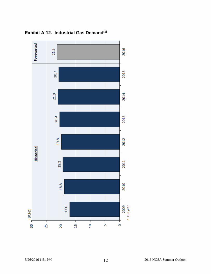
5/26/2016 1:51 PM 2016 NGSA Summer Outlook 12
Exhibit A-12. Industrial Gas Demand(1)

5/26/2016 1:51 PM 2016 NGSA Summer Outlook 13
Exhibit A-13. Capital Expenditures for Plant Expansions (Cumulative)

5/26/2016 1:51 PM 2016 NGSA Summer Outlook 14
Exhibit A-14. Project Count and Impact of Capacity Expansion on Industrial Gas Demand (2015-2020)
Ne
wFe
rtili
zer
11
Stee
l5
Gas
-to
-Liq
uid
s0
Ch
emic
al3
8P
aper
& P
ulp
0To
tal
54
Exp
and
Fert
ilize
r3
Stee
l0
Gas
-to
-Liq
uid
s0
Ch
emic
al1
0P
aper
& P
ulp
0T
ota
l1
3
To
tal P
roje
cts
= 6
7
CO
MP
AR
ISO
N O
F P
RO
JEC
T TY
PE
CO
UN
T FO
R V
AR
IOU
S IN
DU
STR
IES
(20
15
-2
02
0)
Ind
ust
rial
(F
erti
lizer
)3
0%
To
tal =
4.1
BC
FD
Pet
roch
emic
als
69
%
Ind
ust
rial
(Fer
tiliz
er)
29
%
Stee
l1
%
IMP
AC
T O
F C
AP
AC
ITY
EX
PA
NSI
ON
ON
IN
DU
STR
IAL
GA
S D
EMA
ND
(2
01
5 -
20
20
)