Outlines - Kasetsart University · พื้นที่การไหลปลายเข...

203552 Advanced Soil Mechanics 22/08/50

Dr.Warakorn Mairaing 1

1

Dr. Warakorn MairaingDr. Warakorn MairaingAssociate ProfessorAssociate Professor

Civil Engineering DepartmentCivil Engineering DepartmentKasetsart University, Bangkok Kasetsart University, Bangkok Tel: 02Tel: 02--579579--22652265Email: [email protected]: [email protected]

Lecture No. 1

2

OutlinesOutlines1.1. 22--D Flow and Excess Pore PressureD Flow and Excess Pore Pressure

Two Dimensional Flow in SoilTwo Dimensional Flow in SoilSoil Permeability and Pore Pressure MonitoringSoil Permeability and Pore Pressure MonitoringPore Pressure DevelopmentPore Pressure Development

2.2. Soil ConsolidationSoil ConsolidationConcepts of ConsolidationConcepts of ConsolidationTerzaghiTerzaghi’’ss theory of Consolidationtheory of ConsolidationSettlement AnalysesSettlement Analyses

3.3. UndrainedUndrained Shear StrengthShear StrengthFlownetFlownet, Pressure Distribution and Seepage Force, Pressure Distribution and Seepage ForceSoil Permeability and Pore Pressure MonitoringSoil Permeability and Pore Pressure MonitoringPore Pressure DevelopmentPore Pressure Development



3

2-D and 3-D Flow in Soil Mass

Q1 : Why 2-D or 3-D Flows are needed?

A1 : Whenever flow directions are not in 1-direction.

Q2 : Where 2-D or 3-D Flow should be applied?

A2 : Most of the cases in ground water flow.

4



5

6

Saturated Flow

Unsaturated Flow

Steady Flow

Transition Flow

S = 100%

S < 100%

Q = Contant

Q = Contant



7

Drainage, Dewatering

8

Dewatering, Land Subsidence



9

10

0yh

xh

2

2

2

2=

∂∂

+∂∂

0zhk

yhk

xhk 2

2

2

2

2

2.z.y.x =∂∂

+∂∂

+∂∂

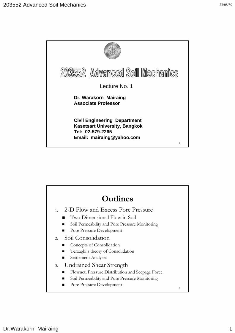
Laplace’s Eqauation สําหรับ 3-D

Laplace’s Eqauation สําหรับ 2-D เม่ือ kx = ky

ดินอ่ิมตัวและการไหลคงที่X

Y

Z dX

dY

dZQ zi

zoQ

yoQ

xiQ

yiQ

xoQ

ความเรว็ของการไหล= Vx

ความเรว็ของการไหล= Vx +c

cVxX.dX



11

12

Steady State Flow (Flow in = Flow Out)

When Qin = Qout is usually occurred in saturated steady flow with no volume change soil mass.

Then Equation (6) become;

Then

0zhk

yhk

xhk 2

2

2

2

2

2.z.y.x =∂∂

+∂∂

+∂∂

---(7)

0=∂∂

tθ



13

Unsteady State Flows (Flow in ≠ Flow out)

When θ = Volume of water in unit volume of soil

( )( )01

.ees

+∂∂

=∂∂

σσθ

---(9)

---(8)

0≠∂∂

tθ

01.eeS

+=θ

14

Substitute in (6), then the general Laplace’s Flow Equation is obtained

---(10)

Considering RHS-Term in Eq. (10), there are 4 possible cases

Case 1 : Both S and e = const. Steady State Flow

Case 2 : S = Const, E Varied Consolidation

Case 3 : S varied, e = Const. Unsaturated flow

Case 4 : S and e varied; Shrinkage and Capillary rising (lowering)

⎟⎠⎞

⎜⎝⎛

∂∂

+∂∂

+=

∂∂

+∂∂

+∂∂

tes

tSe

ezhk

yhk

xhk zyx ..

11...

02

2

2

2

2

2



15

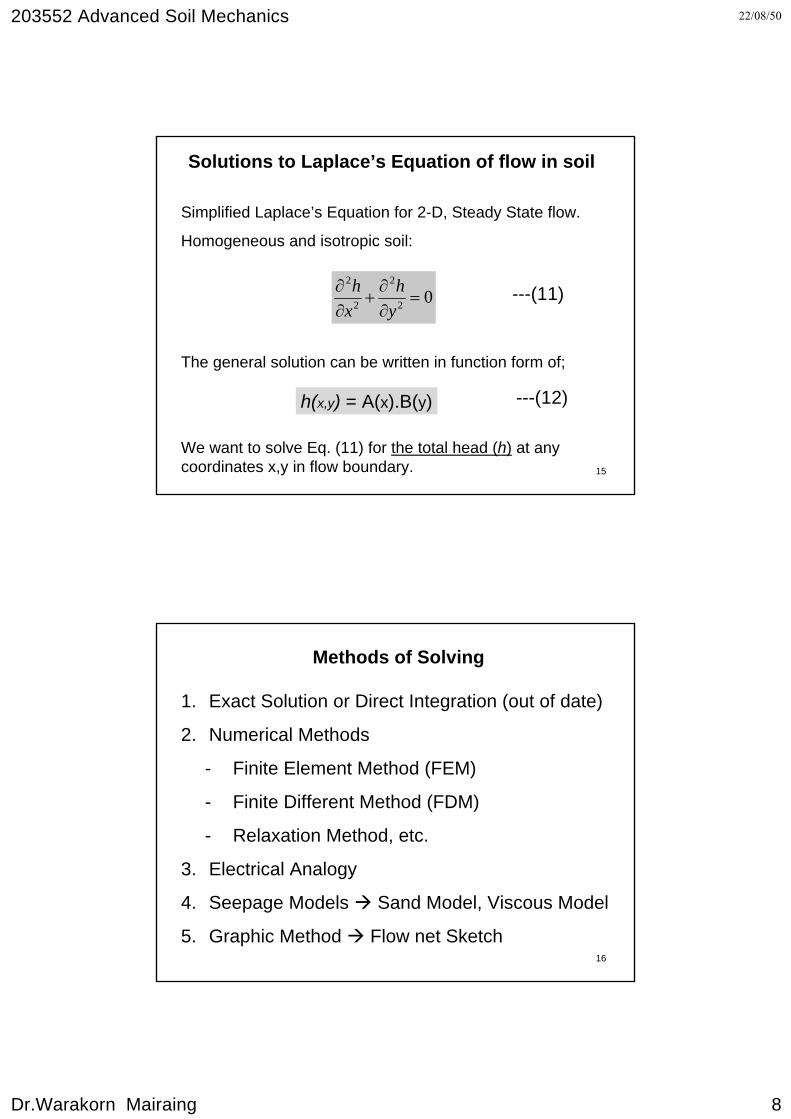
Solutions to Laplace’s Equation of flow in soil

Simplified Laplace’s Equation for 2-D, Steady State flow.

Homogeneous and isotropic soil:

02

2

2

2

=∂∂

+∂∂

yh

xh

The general solution can be written in function form of;

h(x,y) = A(x).B(y)

We want to solve Eq. (11) for the total head (h) at any coordinates x,y in flow boundary.

---(11)

---(12)

16

Methods of Solving

1. Exact Solution or Direct Integration (out of date)

2. Numerical Methods

- Finite Element Method (FEM)

- Finite Different Method (FDM)

- Relaxation Method, etc.

3. Electrical Analogy

4. Seepage Models Sand Model, Viscous Model

5. Graphic Method Flow net Sketch



17

Outline of Exact Solution See More Detail in Advanced Soil Mechanics by B.M. DAS (P102-120)

18

Solution Form



19

2-D v.s. 3-D Flows

Normally engineers would like to simplified flow problems from 3-D to 2-D. When ever the problems can be accepted with the reasonable accuracy.

For 2-D Steady state flow;

0.. 2

2

2

2

=∂∂

+∂∂

yhk

xhk yx ---(15)

20

Validity of 2-D Flow Cases



21

22



23

24



25

26

การวิเคราะหการไหลซึมดวยวิธี Relaxation ผลจากการวิเคราะหดวยวิธี Relaxation

การใชการไหลของกระแสไฟฟาแทนการไหลของน้ํา



27

Relaxation Method

การวิเคราะหการไหลซึมดวยวิธี Relaxation

28

1. กริดภายใน Flow B

การไหลตามแนวแกน x จากจุด 3 0 1

3030

03 ahh

xh i=

−=

→∂∂

จาก 0 1

จาก 3 0

0101

01 ahh

xh i=

−=

∂∂



29

20313001

3012

2 2a

xh

xh

x

h a

hhh −+=

−=

∂∂

∂∂

∂

∂

2042

4022

2

a2hhh

y h −+

=∂∂

อัตราการเปลี่ยนแปลงของ Hydraulic gradient จากจุดกึ่งกลาง ดาน 3-0 และ 0-1 คือ

ทํานองเดียวกัน

30

0a

4hhhhh2

042312

2

2

2

=−+++

=∂∂

+∂∂

∴yh

xh

oh4hhhh4321

=+++หรือ

ตัวคูณน้ําหนักการกระจายของศักยน้ํา

“สมการควบคุม”



31

“สมการควบคุม”hshhh 222 786 =++

พ้ืนที่การไหลชิดขอบทึบน้ํา

ก) พ้ืนที่การไหล ข) การกระจายน้ําหนักของศักยน้ํา

32

ก. พ้ืนที่การไหลปลายเข็มพืด

ข. พ้ืนที่การไหลมุมของขอบทึบน้ํา

พื้นที่การไหลปลายเข็มพืดและพื้นทีการไหลมุมขอบทึบน้ํา



33

จะเห็นไดวา “ศักยน้ํา” (h) ณ จุดตางๆ ในบริเวณพื้นที่กริดใดๆ จะถูกตองตามสมการ Laplace’s ไดก็ตอเมื่อคา “h” มีความสัมพันธกันตาม “สมการควบคุม” ของพื้นที่นั้นๆ

หากไมเปนดังกลาวกลาวจะเกิด Error ขึ้น ซึ่งจะตองกระจายไปตามน้ําหนักการกระจายศักยที่เขียนไวในแผนภูมิ

34

ตัวอยางการกระจาย Error ของพื้นที่การไหลที่ขอบทึบน้ํา

ถา h15 = 14.5 ม. h16 = 13.0 ม.h17 = 15.2 ม. h18 = 15.0 ม.h19 = 13.5 ม.

สมการควบคุม

1519181716 322

hhhhh=+++ 5.1435.130.15

02.15

20.13

×=+++

∴Error ขางขวามากกวาขางซาย = 43.5 – 42.6=0.9 แบง Error ออกเปน 6 สวน (0.5+0.5+1+1+3) ไดสวนละ = 0.15นําสวนแบงของ Error = 0.15 ไปปรับให h15 ลดลง 1 สวน = 14.5-0.15=14.35h16, h17, h18, h19 เพิ่มขึ้น 1 สวน

42.6 43.5



35การใชการไหลของกระแสไฟฟาแทนการไหลของน้ํา

การเปรียบเทียบการไหลของน้ําและกระแสไฟฟา¡ÒÃäËÅ¢Í§¹éÓ ¡ÒÃäËÅ¢Í§¡ÃÐáÊä¿¿éÒ

Total head, h Voltage, vPermeability, k Electrical conductivity, CDischarge velocity, v Current, IDarcy's law Ohm's lawvkhL=−ΔΔ ICVL=−ΔΔ

ÊÁ¡ÒÃ∂∂∂∂hxhy02222+=

ÊÁ¡ÒÃ ∂∂∂∂ϖξϖψ02222+=

36

Seepage Tank

Hele Shaw Model Viscons flolw

การจําลองการไหลดวยถังทราย

การจําลองการไหลดวยแบบจําลองน้ํามัน



37

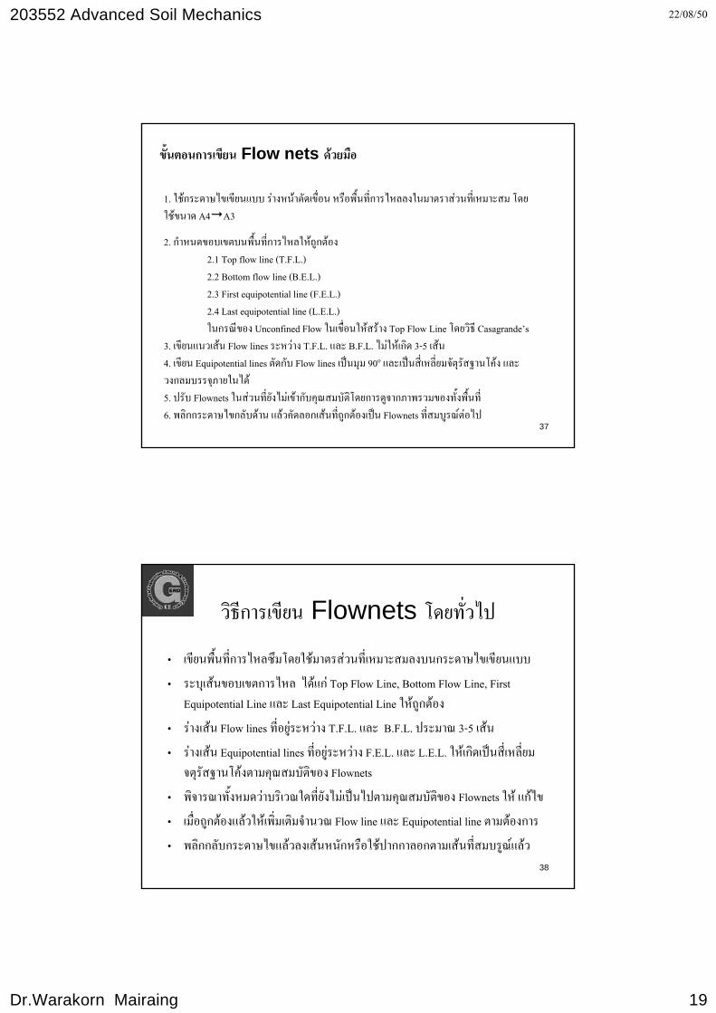
ขั้นตอนการเขียน Flow nets ดวยมือ

1. ใชกระดาษไขเขยีนแบบ รางหนาตัดเขื่อน หรือพื้นที่การไหลลงในมาตราสวนทีเ่หมาะสม โดยใชขนาด A4 A3

2. กําหนดขอบเขตบนพื้นที่การไหลใหถูกตอง2.1 Top flow line (T.F.L.)2.2 Bottom flow line (B.E.L.)2.3 First equipotential line (F.E.L.)2.4 Last equipotential line (L.E.L.)ในกรณีของ Unconfined Flow ในเขื่อนใหสราง Top Flow Line โดยวิธี Casagrande’s

3. เขียนแนวเสน Flow lines ระหวาง T.F.L. และ B.F.L. ไมใหเกิด 3-5 เสน4. เขียน Equipotential lines ตัดกับ Flow lines เปนมุม 90o และเปนสี่เหลี่ยมจัตุรัสฐานโคง และวงกลมบรรจุภายในได5. ปรับ Flownets ในสวนที่ยงัไมเขากับคุณสมบัติโดยการดูจากภาพรวมของทั้งพื้นที่6. พลิกกระดาษไขกลับดาน แลวคัดลอกเสนที่ถูกตองเปน Flownets ที่สมบูรณตอไป

38

วิธีการเขียน Flownets โดยทั่วไป

• เขียนพื้นที่การไหลซึมโดยใชมาตรสวนที่เหมาะสมลงบนกระดาษไขเขียนแบบ

• ระบุเสนขอบเขตการไหล ไดแก Top Flow Line, Bottom Flow Line, First Equipotential Line และ Last Equipotential Line ใหถูกตอง

• รางเสน Flow lines ที่อยูระหวาง T.F.L. และ B.F.L. ประมาณ 3-5 เสน

• รางเสน Equipotential lines ที่อยูระหวาง F.E.L. และ L.E.L. ใหเกิดเปนสี่เหลี่ยม จตุรัสฐานโคงตามคุณสมบัติของ Flownets

• พิจารณาทั้งหมดวาบริเวณใดที่ยังไมเปนไปตามคุณสมบัติของ Flownets ให แกไข

• เมื่อถูกตองแลวใหเพิ่มเติมจํานวณ Flow line และ Equipotential line ตามตองการ

• พลิกกลับกระดาษไขแลวลงเสนหนักหรือใชปากกาลอกตามเสนที่สมบรูณแลว



39

ขั้นตอนการเขียน FlownetsA B C D

Z

X

Y

First Equipotential Line Last Equipotential Line

Sheet Pile

First Equipotential Line

Top Flow Line

A B C D

ZY

First Equipotential Line Last Equipotential Line

Sheet Pile

A B C D

ZY

Sheet Pile

1. สราง Boundary Lines

2. สราง Flow lines และ Equipotential lines เร่ิมตน

3. แกไขใหเขาคุณสมบตัิของ Flownets

40

ตัวอยางการเขียนFlownets

Flow into Coffer Dam

Flow under Weir

Flow into Drain Pipe



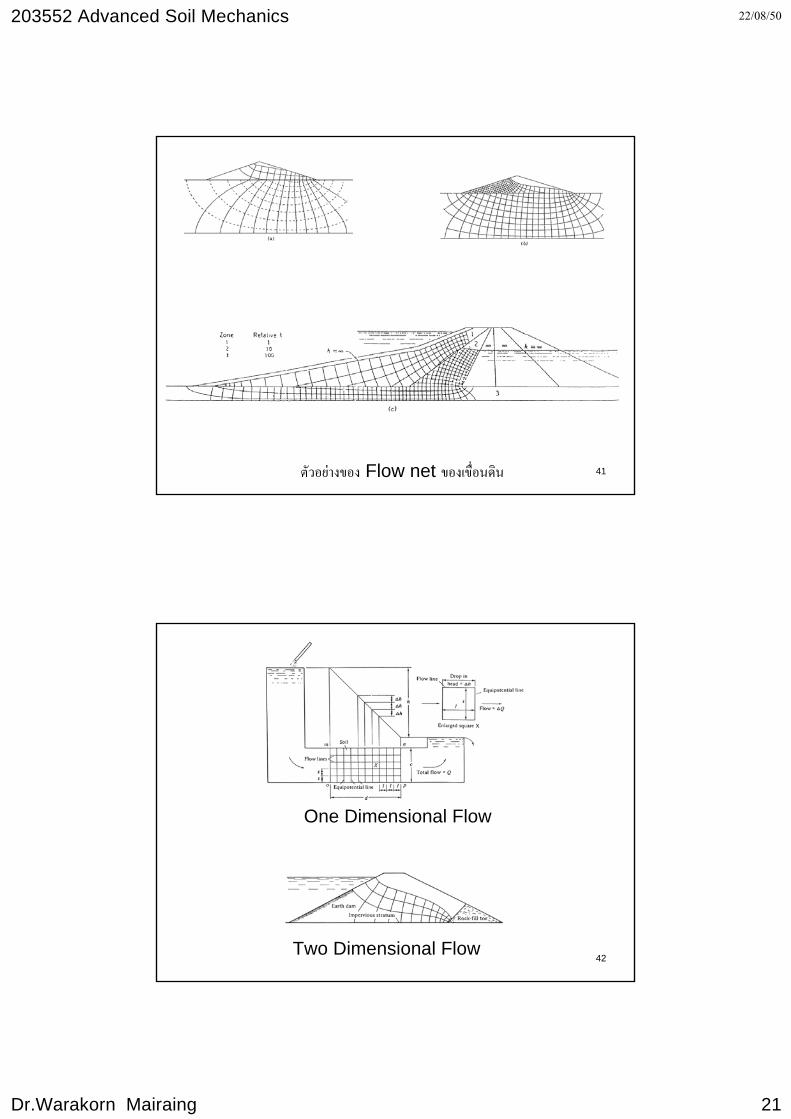
41ตัวอยางของ Flow net ของเขื่อนดิน

42

One Dimensional Flow

Two Dimensional Flow



43

Anisotropic Flow; when kx ≠ky

1. Compacted Soil

- Compaction by Sheepfoot kH ≈ 4 kv

- Compaction by Rubber tyre roller kH ≈ 20 kv

2. Sediment Soil

- Layered soil kH ≈ 20 – 200 kv

44

Flow lines at soil interface



45

46

ผลของอัตราสวนของคาความซึมน้ําท่ีมีตอความมั่นคงของลาดเขื่อน



47

48

F.E.P L.E.P

T.F.L

B.F.L

Concreteweir

A B C D

E

FG

H I

Δ QΔ Q

Δ Q

Δ h

Δ h Δ h



49

ααα

22min

22max

2min

2max2

.cosk.sink

.kkk+

=

ความแตกตางของคาความซึมน้ําแทนดวย Elipse of Direction

minmaxav .k kk=

50



51

ช้ันดินที่มีคาความซึมน้ําตางกันตามทิศทาง

คาความซึมน้ําที่เปล่ียนแปลงตามทิศทาง

52

Flow nets Sketch for Anisotropic Soil



53

Non-homogeneous Flow in Soils

Cause concentration of flow in some loayer and uplift pressure on another layer

Other effects to flow problems

- Perched water table

- Artesian water table

54



55

56



57

58



59

60



61

62

การคาํนวณแรงดันน้ําจาก Flownets

( ) eiitopi hh.nhh −Δ−=

เมื่อ =toh ศักยรวมเร่ิมตน =Δh ศักยท่ีสญูเสยีในชวง Equipotential Space in = จํานวน Equipotential Space จากจุดเริ่มตนไปถึงจุด I ใดๆ eih = ศักยความสงูของจุด I ใดๆ



63

การคํานวณความดันน้ําจาก Flownets

0.50.50.017.510.018.0112.22.20.115.79.018.0103.83.80.214.08.018.095.35.30.512.27.018.086.56.51.010.56.018.077.07.02.38.75.018.066.56.54.57.04.018.055.35.37.55.23.018.043.53.511.03.52.018.031.31.315.01.71.018.020.00.018.00.00.018.01

ui(ตัน/ตร.ม.)

hpi(เมตร)

hei(เมตร)

ni.Δh

(เมตร)ni

(ชอง)hT0

(เมตร)

จุดที่

64



65

66

Hydraulic Gradient (C)

On flow boundary at any point (x) hydraulic gradient (ii) equal to

Lhii Δ

Δ=

xx l

hiΔΔ

=

yy l

hiΔΔ

=

xyxy iill >→∴Δ<ΔSeepage velocity (v)

xx kiv = ---(5)

---(4)

yy kiv =and



67

Seepage Force and Boiling

UWb (boiling) F.S. =

Ah..v.A.Hv

w

b= ---(6)If boiling occurring

68

Thenw

b

w

b

vv

hh

hH

vv

=→−=1

Then F.S. = 1,



69

Seepage Quantity (Q)

70


1. Estimation of seepage loss- Reservior (Dam)- Leachet from sanitary landfill

2. Pumping and drainage capacity- Filter Design- Dewatering

From Darcy’s law

v = ki

Q = kiAor ---(1)



71

for 1 - flow channel

1... fllehkQ Δ

=Δ ---(2)


Any flow spacerNehhandlle f =Δ≈

NehkQ .=Δ∴

---(4)

Summation of every flow channels, Q = ΣΔQ

hkNN

QNQc

ff ... =Δ=

---(3)

72

Homework



73

74



75

76



77

Outlines - Kasetsart University · พื้นที่การไหลปลายเข...

Documents

Transcript of Outlines - Kasetsart University · พื้นที่การไหลปลายเข...