OUTLINE

Introduction to Analogous System.

Force-Voltage Analogy.

Force-Current Analogy.

Example on Analogous System.

Mechanical Equivalent Network.

SYED HASAN SAEED 1

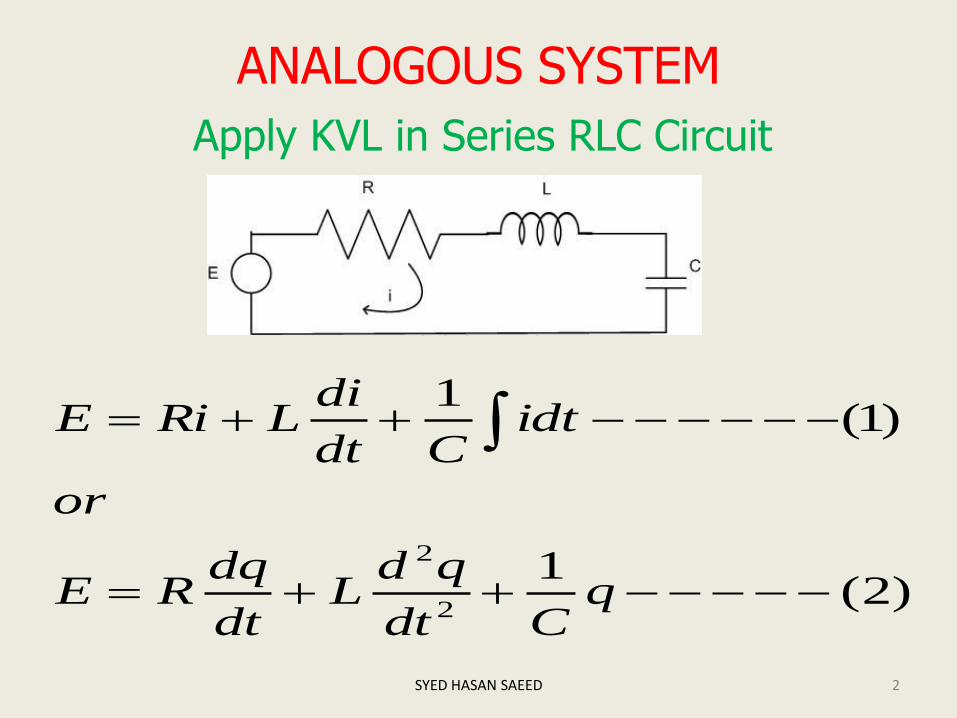
ANALOGOUS SYSTEM

Apply KVL in Series RLC Circuit

aaanna

SYED HASAN SAEED

)2(1

)1(1

2

2

qCdt

qdL

dt

dqRE

or

idtCdt

diLRiE

2

Consider parallel RLC circuit and apply KCL

SYED HASAN SAEED

)4(1

)(1

,

)3(1

2

2

dt

dC

Ldt

d

RI

dt

dEEdt

dt

dECEdt

LR

EI

3

We know the equation of mechanical system

Compare equation(5) with equation(2)

FORCE –VOLTAGE ANALOGY (f-v)

SYED HASAN SAEED

)5()()()(

)(2

2

tKxdt

tdxB

dt

txdMtF

S.NO. TRANSLATIONAL SYSTEM ELECTRICAL SYSTEM

1. Force (F) Voltage (E)

2. Mass (M) Inductance (L)

3. Stiffness (K), Elastance (1/K)

Reciprocal of C, Capacitance (C)

4. Damping coefficient (B) Resistance (R)

5. Displacement (x) Charge (q) 4

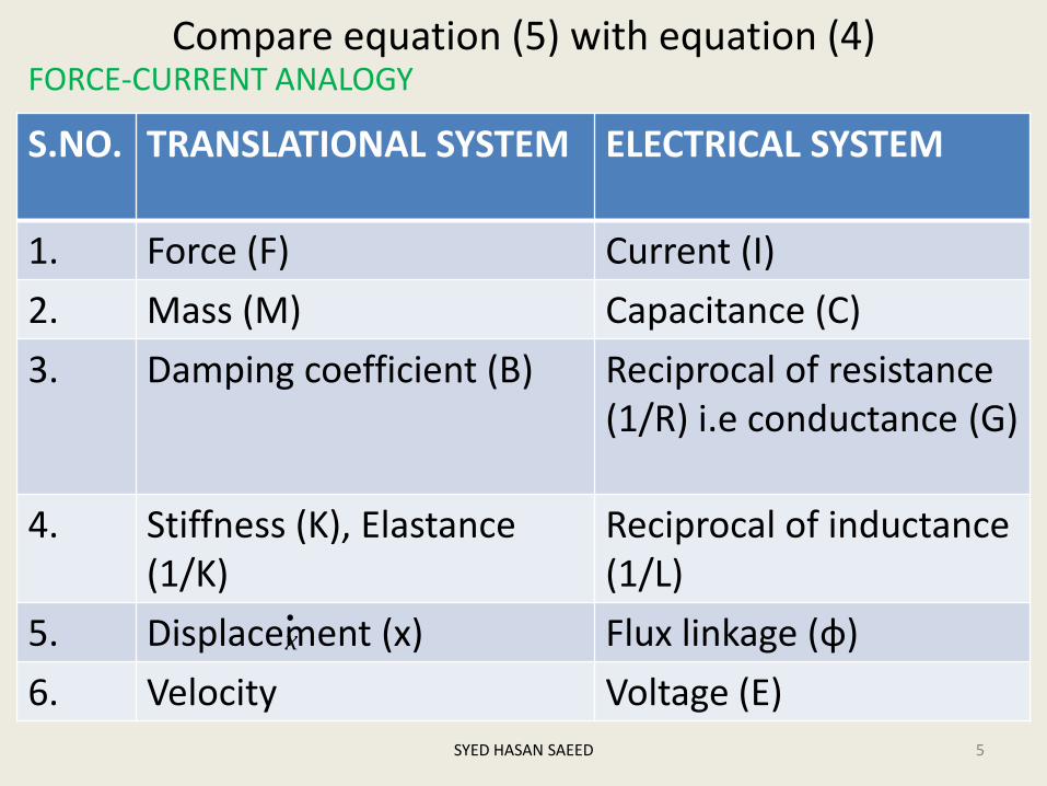
Compare equation (5) with equation (4) FORCE-CURRENT ANALOGY

SYED HASAN SAEED

S.NO. TRANSLATIONAL SYSTEM ELECTRICAL SYSTEM

1. Force (F) Current (I)

2. Mass (M) Capacitance (C)

3. Damping coefficient (B) Reciprocal of resistance (1/R) i.e conductance (G)

4. Stiffness (K), Elastance (1/K)

Reciprocal of inductance (1/L)

5. Displacement (x) Flux linkage (φ)

6. Velocity Voltage (E)

x

5

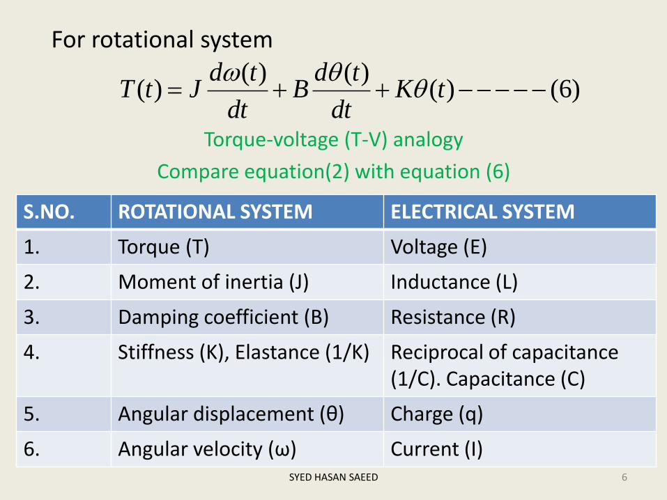
For rotational system

Torque-voltage (T-V) analogy

Compare equation(2) with equation (6)

SYED HASAN SAEED 6

)6()()()(

)( tKdt

tdB

dt

tdJtT

S.NO. ROTATIONAL SYSTEM ELECTRICAL SYSTEM

1. Torque (T) Voltage (E)

2. Moment of inertia (J) Inductance (L)

3. Damping coefficient (B) Resistance (R)

4. Stiffness (K), Elastance (1/K) Reciprocal of capacitance (1/C). Capacitance (C)

5. Angular displacement (θ) Charge (q)

6. Angular velocity (ω) Current (I)

Compare equation (4) with equation (6)

TORQUE(T)-CURRENT (I) ANALOGY

SYED HASAN SAEED 7

S.NO. ROTATIONAL SYSTEM ELECTRICAL SYSTEM

1. Torque (T) Current (I)

2. Moment of inertia (J) Capacitance (C)

3. Damping coefficient (B) Reciprocal of resistance (R), conductance (G)

4. Stiffness (K), Elastance (1/K) Reciprocal of inductance (1/L)

5. Angular displacement (ω) Flux linkage (φ)

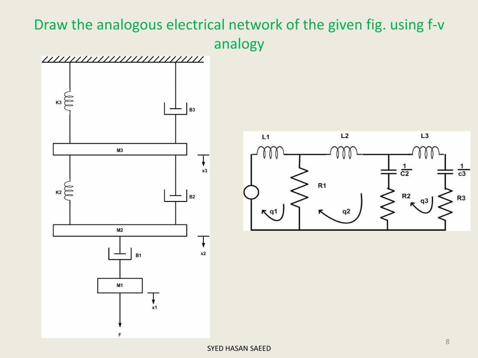
Draw the analogous electrical network of the given fig. using f-v analogy

SYED HASAN SAEED 8

MECHANICAL EQUIVALENT NETWORK

PROCEDURE TO DRAW THE MECHANICAL EQUVALENT NETWORK:

Step 1: Draw a reference line.

Step 2: Corresponding to the displacement x1 x2 ….select the nodes.

Step 3: Connect one end of masses to the reference line

Step 4: Connect other elements of the system to the nodes.

Step 5: Apply nodal analysis, write the system equations.

SYED HASAN SAEED 9

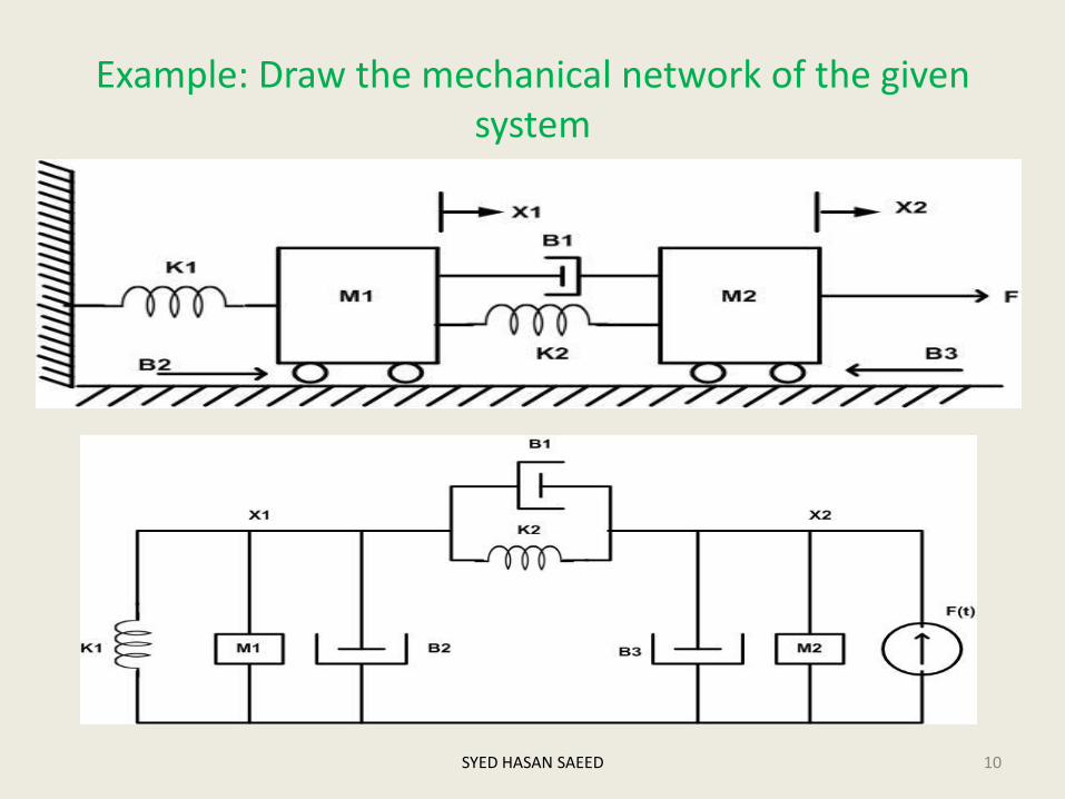
Example: Draw the mechanical network of the given system

SYED HASAN SAEED 10

THANK YOU FOR YOUR ATTENTION

SYED HASAN SAEED 11

OUTLINE

Advantages and disadvantages of block diagram.

Terminology.

Closed loop.

How to draw the block diagram.

Block reduction Technique.

SYED HASAN SAEED 1

BLOCK DIAGRAM REPRESENTATION

BLOCK DIAGRAM:

a. Block diagram is a pictorial representation of the system.

b. Block diagram represent the relationship between input and output.

c. Any complicated system can be represented by connecting the different block.

d. Each block is completely characterized by a transfer function.

SYED HASAN SAEED 2

ADVANTAGES OF BLOCK DIAGRAM:

a. A block may represent a single component or a group of components.

b. Performance of a system can be determined by block diagram.

c. Block diagram is helpful for designing and analysis of a system.

d. Construction of block diagram is simple for any complicated system.

e. The operation of any system can be easily observed by block diagram representation.

SYED HASAN SAEED 3

DISADVANTAGES OF BLOCK DIAGRAM:

a. Source of energy is not shown in the diagram.

b. Block diagram does not give any information about the physical construction of the system.

c. Applicable only for linear time invariant system.

d. It requires more time.

e. It is not a systematic method.

f. For a given system, the block diagram is not unique.

SYED HASAN SAEED 4

Following figure shows the different components of block diagram

Input R(s) C(s) output

The arrow pointing towards block indicates input R(s) and arrow head leading away from the block represent the output C(s).

or

SYED HASAN SAEED 5

Transfer Function G(S)

)(

)()(

sR

sCsG )()()( sRsGsC

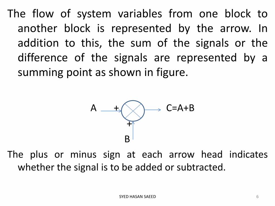
The flow of system variables from one block to another block is represented by the arrow. In addition to this, the sum of the signals or the difference of the signals are represented by a summing point as shown in figure.

A + C=A+B

+

B

The plus or minus sign at each arrow head indicates whether the signal is to be added or subtracted.

SYED HASAN SAEED 6

Application of one input source to two or more block is represented by a take off point. Take off point also known as branch point, shown below

Forward path: The direction of flow of signal from input to output.

Feedback path: The direction of flow of signal is from output to input.

SYED HASAN SAEED 7

G1

G2

BLOCK DIAGRAM OF A CLOSED LOOP SYSTEM

r(t) = reference input signal

c(t)= controlled output

e(t)= error signal

b(t)= feedback signal

R(s)=Laplace transform of input

C(s)= Laplace transform of output

B(s) Laplace transform of feedback signal

E(s) Laplace transform of error signal

Block diagram

C(s)

SYED HASAN SAEED 8

G(s)

H(s)

From the figure

The error signal is

From above equations we get

SYED HASAN SAEED 9

)2_________()()()(

)1_________()()()(

sHsCsB

sEsGsC

)()()( sBsRsE

)3______(__________)()(1

)(

)(

)(

)()()()(1)(

)()()()()()(

)()()()()(

)()()()(

sHsG

sG

sR

sC

sHsGsHsGsC

sCsHsGsRsGsC

sBsGsRsGsC

sBsRsGsC

Equation (3) is for negative feedback.

For positive feedback equation (3) becomes

SYED HASAN SAEED 10

)()(1

)(

)(

)(

sHsG

sG

sR

sC

HOW TO DRAW BLOCK DIAGRAM ?

Draw the block diagram of the given circuit.

SYED HASAN SAEED 11

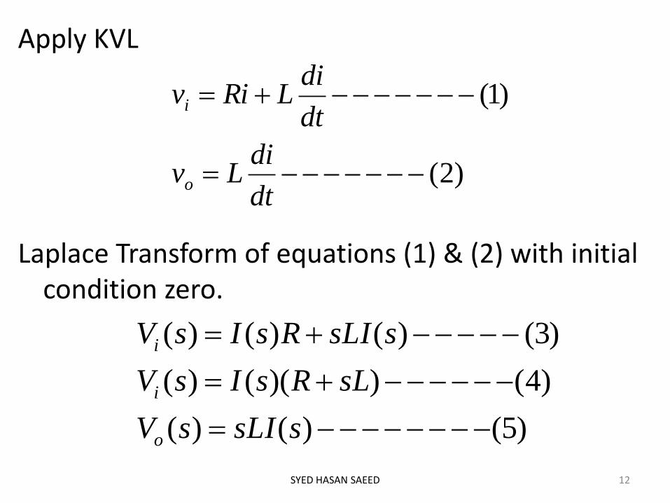
Apply KVL

Laplace Transform of equations (1) & (2) with initial condition zero.

SYED HASAN SAEED 12

)2(

)1(

dt

diLv

dt

diLRiv

o

i

)5()()(

)4())(()(

)3()()()(

ssLIsV

sLRsIsV

ssLIRsIsV

o

i

i

From equations (4) & (5)

From fig.

Laplace transform of above equations

SYED HASAN SAEED 13

)7(

)6(

dt

diLv

R

vvi

o

oi

)9()()(

)8()()(1

)(

ssLIsV

sVsVR

sI

o

oi

sLR

sL

sV

sV

i

o

)(

)(

Vi(s) Vi(s)-Vo(s) I(s)

+

-

Vo(s)

SYED HASAN SAEED 14

1/R

SYED HASAN SAEED 15

BLOCK DIAGRAM REDUCTION

SYED HASAN SAEED 16

Drive the transfer function using block reduction technique.

Step1: There are two internal closed loop, remove these loops by using closed loop formula

SYED HASAN SAEED 17

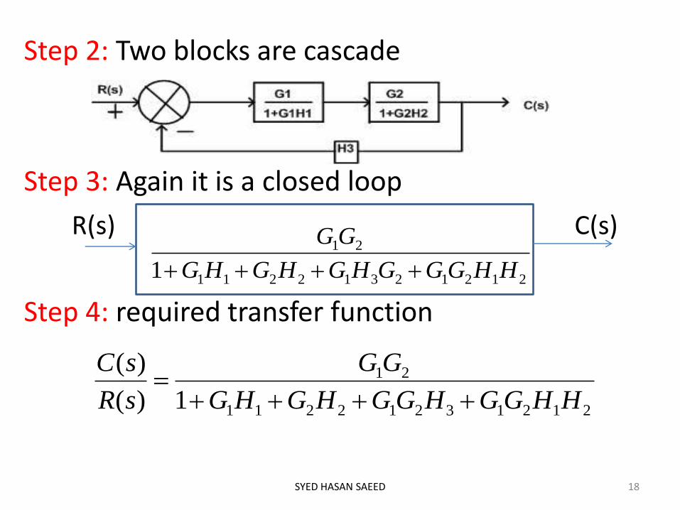
Step 2: Two blocks are cascade

Step 3: Again it is a closed loop

R(s) C(s)

Step 4: required transfer function

SYED HASAN SAEED 18

21212312211

21

1 HHGGGHGHGHG

GG

21213212211

21

1)(

)(

HHGGHGGHGHG

GG

sR

sC

THANK YOU

SYED HASAN SAEED 19

AUTOMATIC CONTROL SYSTEMS

BOOKS

1. CONTROL SYSTEM B.C. KUO

2. CONTROL SYSTEMS K. OGATTA

3. CONTROL SYSTEMS NAGRATH & KOTHARI

4. AUTOMATIC CONTROL SYSTEMS S.HASAN SAEED

SYED HASAN SAEED 1

OUTLINE

Basic definitions.

Requirement of control systems.

Classification of control systems.

Open loop and closed loop control systems.

Comparison of open loop and closed loop systems.

Components of closed loop system

SYED HASAN SAEED 2

INTRODUCTION TO CONTROL SYSTEMS

BASIC DEFINITIONS

SYSTEM : A system is collection of or combination of objects or components connected together in such a manner to attain a certain objective.

OUTPUT : The actual response obtained from a system is called output.

INPUT: The excitation applied to a control system from an external source in order to produce the output is called input.

CONTROL: Control means to regulate, direct or command a system so that the desired objective is obtained.

SYED HASAN SAEED 3

CONTROL SYSTEM: A control system is a system in which the output quantity is controlled by varying the input quantity.

REQUIREMENT OF A GOOD CONTROL SYSTEM:

(i) Accuracy: Accuracy is high as any error arising should be corrected. Accuracy can be improved by using feedback element. To increase accuracy error detector should be present in control system.

(ii) Sensitivity: Control system should be insensitive to environmental changes, internal disturbances or any other parameters.

SYED HASAN SAEED 4

(iii) Noise: Noise is an undesirable input signal. Control system should be insensitive to such input signals.

(iv) Stability: In the absence of the inputs, the output should tend to zero as time increases. A good control system should be stable.

(iv) Stability: In the absence of the inputs, the output should tend to zero as time increases. A good control system should be stable.

SYED HASAN SAEED 5

• (v) Bandwidth: The range of operating frequency decides the bandwidth. For frequency response bandwidth should be large.

• (vi) Speed: The speed of control system should be high.

• (vii) Oscillations: For good control system, oscillation should be constant or sustained oscillation which follows the Barkhausein’s criteria.

SYED HASAN SAEED

6

CLASSIFICATION OF CONTROL SYSTEMS

Depending upon the purpose control system can be classified as follows (ref. Control systems by A. Anand Kumar)

1. Depending on hierarchy:

(i) Open loop control systems

(ii) Closed loop control systems

(iii) Adaptive control systems

(iv) Learning control systems

2. Depending on the presence of Human being as apart of the control system

(i) Manually control systems (ii) Automatic control systems

SYED HASAN SAEED 7

3. Depending on the presence of feedback

(i) Open loop control systems

(ii) Closed loop control systems or feedback control systems.

4. According to the main purpose of the system

(i) Position control systems

(ii) Velocity control systems

(iii)Process control systems

(iv) Temperature control systems

(v) Traffic control systems etc.

SYED HASAN SAEED 8

Feedback control systems may be classified as

(i) linear control systems and nonlinear control systems.

(ii) Continuous data control systems and discrete data control systems , ac (modulated) control systems and dc (unmodulated) control systems.

(iii)Multi input multi output(MIMO) system and single input single output (SISO) systems.

(iv) Depending upon the number of poles of the transfer function at the origin, systems may be classified as Type-0, Type-1, Type-2 systems etc.

SYED HASAN SAEED 9

(v) Depending on the order of the differential equation, control systems may be classified as first order system, second order system etc.

(vi) According to type of damping control systems may be classified as Undamped control systems, damped control systems, Critically damped control systems and Overdamped control systems.

SYED HASAN SAEED 10

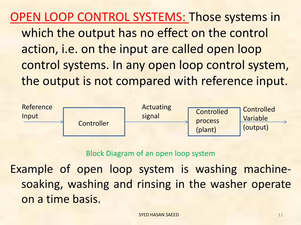
OPEN LOOP CONTROL SYSTEMS: Those systems in which the output has no effect on the control action, i.e. on the input are called open loop control systems. In any open loop control system, the output is not compared with reference input.

Block Diagram of an open loop system

Example of open loop system is washing machine-soaking, washing and rinsing in the washer operate on a time basis.

SYED HASAN SAEED

Controller

Controlled process (plant)

Actuating signal

Reference Input

Controlled Variable (output)

11

CLOSED LOOP CONTROL SYSTEM: Closed loop control systems are also known as feedback control systems. A system that maintains a prescribed relationship between the output and reference input by comparing them and using the difference as a mean of control is called feedback control system.

Example of feedback control system is a room temperature control system. By measuring the room temperature and comparing it with the desired temperature, the thermostat turns the cooling or heating equipment on or off.

SYED HASAN SAEED 12

Block Diagram of a Closed Loop System

SYED HASAN SAEED

Controller Plant

Feedback Path Element

Error Signal

Actuating signal Output Ref.

Input

Feedback Signal

+ -

13

OPEN LOOP SYSTEM v/s CLOSED LOOP SYSTEM

SYED HASAN SAEED

S.NO. OPEN LOOP SYSTEM CLOSED LOOP SYSTEM

1. These are not reliable These are reliable

2. It is easier to build It is difficult to build

3. They Consume less power

They Consume more power

4. They are more stable These are less stable

5. Optimization is not possible

Optimization is possible

14

COMPONENTS OF CLOSED LOOP SYSTEMS

SYED HASAN SAEED

Controlled system

Controlled Element

Feedback Element

Command Input

Ref. Input Element

+

- +

15

Command: The command is the externally produced input and independent of the feedback.

Reference input element: This produces the standard signals proportional to the command.

Control element: This regulate the output according to the signal obtained from error detector.

Controlled System: This represents what we are controlling by the feedback loop.

Feedback Element: This element fed back the output to the error detector for comparison with the reference input.

SYED HASAN SAEED 16

THANK YOU

FOR

YOUR ATTENTION

SYED HASAN SAEED 17

SIGNAL FLOW GRAPH

(SFG)

SYED HASAN SAEED 1

OUTLINE

Introduction to signal flow graph. Definitions

Terminologies

Properties

Examples

Mason’s Gain Formula.

Construction of Signal Flow Graph.

Signal Flow Graph from Block Diagram.

Block Diagram from Signal Flow Graph.

Effect of Feedback.

SYED HASAN SAEED 2

INTRODUCTION

• SFG is a simple method, developed by S.J.Mason

• Signal Flow Graph (SFG) is applicable to the linear systems.

• It is a graphical representation.

• A signal can be transmitted through a branch only in the direction of the arrow.

SYED HASAN SAEED 3

Consider a simple equation

y= a x

The signal Flow Graph of above equation is shown below

a

x y

Each variable in SFG is designed by a Node.

Every transmission function in SFG is designed by a branch.

Branches are unidirectional.

The arrow in the branch denotes the direction of the signal flow.

SYED HASAN SAEED 4

TERMINOLOGIES

SYED HASAN SAEED 5

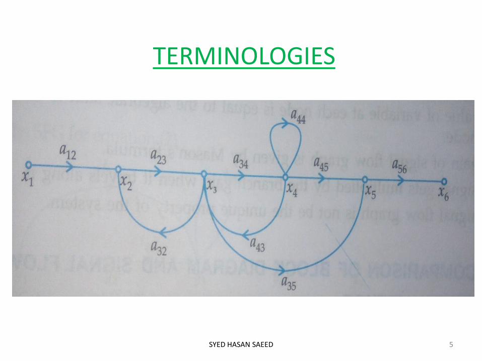
Input Node or source node: input node is a node which has only outgoing branches. X1 is the input node.

Output node or sink node: an output node is a node that has only one or more incoming branches. X6 is the output node.

Mixed nodes: a node having incoming and outgoing branches is known as mixed nodes. x2, x3, x4 and x5 are the mixed nodes.

Transmittance: Transmittance also known as transfer function, which is normally written on the branch near arrow.

SYED HASAN SAEED 6

Forward path: Forward path is a path which originates from the input node and terminates at the output node and along which no node is traversed more than once. X1-x2-x3-x4-x5-x6 and x1-x2-x3-x5-x6 are forward paths.

Loop: loop is a path that originates and terminates on the same node and along which no other node is traversed more than once. e.g x2 to x3 to x2 and x3 to x4 to x3 .

Self loop: it is a path which originates and terminates on the same node. For example x4

SYED HASAN SAEED 7

SYED HASAN SAEED 8

Path gain: The product of the branch gains along the path is called path gain. For example the gain of the path x1-x2-x3-x4-x5-x6 is a12a23a34a45a56

Loop Gain: The gain of the loop is known as loop gain.

Non-touching loop: Non-touching loops having no common nodes branch and paths. For example x2

to x3 to x2 and x4 to x4 are non-touching loops.

PROPERTIES OF SIGNAL FLOW GRAPH:

1. Signal flow graph is applicable only for linear time-invariant systems.

2. The signal flow graph along the direction of the arrow.

3. The gain of the SFG is given by Mason’s formula.

4. The signal gets multiplied by branch gain when it travels along it.

5. The SFG is not be the unique property of the sytem.

6. Signal travel along the branches only in the direction described by the arrows of the branches.

SYED HASAN SAEED 9

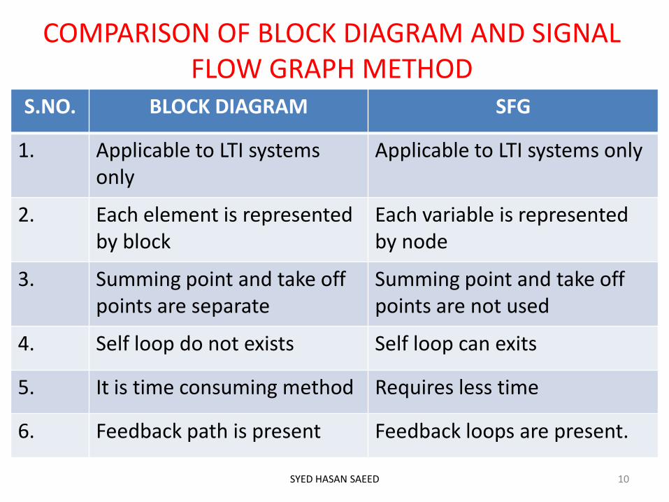
COMPARISON OF BLOCK DIAGRAM AND SIGNAL FLOW GRAPH METHOD

S.NO. BLOCK DIAGRAM SFG

1. Applicable to LTI systems only

Applicable to LTI systems only

2. Each element is represented by block

Each variable is represented by node

3. Summing point and take off points are separate

Summing point and take off points are not used

4. Self loop do not exists Self loop can exits

5. It is time consuming method Requires less time

6. Feedback path is present Feedback loops are present.

SYED HASAN SAEED 10

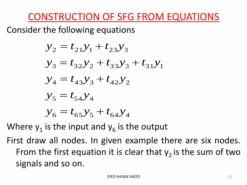
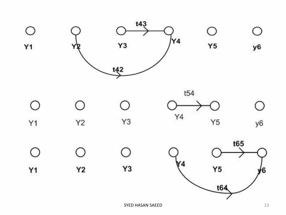
CONSTRUCTION OF SFG FROM EQUATIONS Consider the following equations

Where y1 is the input and y6 is the output

First draw all nodes. In given example there are six nodes. From the first equation it is clear that y2 is the sum of two signals and so on.

SYED HASAN SAEED 11

4645656

4545

2423434

1313332323

3231212

ytyty

yty

ytyty

ytytyty

ytyty

SYED HASAN SAEED 12

SYED HASAN SAEED 13

Complete Signal Flow Graph

SYED HASAN SAEED 14

CONSTRUCTION OF SFG FROM BLOCK DIAGRAM

All variables, summing points and take off points are represented by nodes.

If a summing point is placed before a take off point in the direction of signal flow, in such case represent the summing point and take off point by a single node.

If a summing point is placed after a take off point in the direction of signal flow, in such case represent the summing point and take off point by separate nodes by a branch having transmittance unity.

SYED HASAN SAEED 15

SYED HASAN SAEED 16

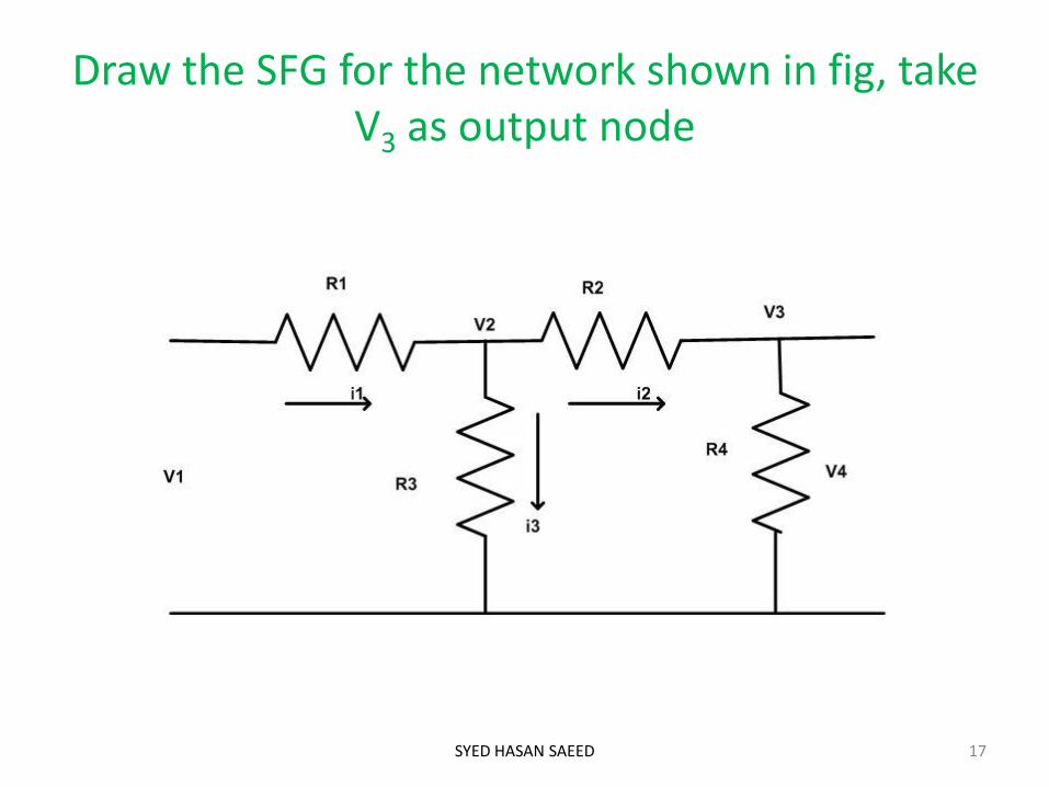
Draw the SFG for the network shown in fig, take V3 as output node

SYED HASAN SAEED 17

SYED HASAN SAEED 18

243

2

3

2

22

2313213332

1

2

1

11

)(

iRv

R

v

R

vi

iRiRiiRRiv

R

v

R

vi

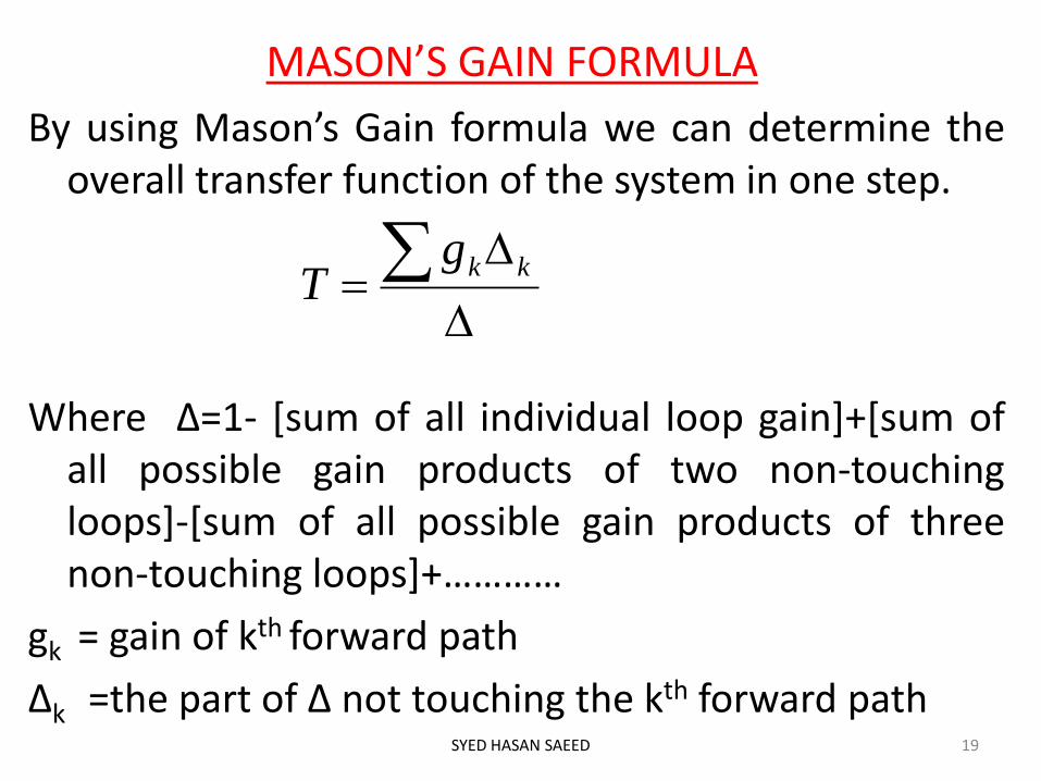
MASON’S GAIN FORMULA

SYED HASAN SAEED 19

By using Mason’s Gain formula we can determine the overall transfer function of the system in one step.

Where Δ=1- [sum of all individual loop gain]+[sum of all possible gain products of two non-touching loops]-[sum of all possible gain products of three non-touching loops]+…………

gk = gain of kth forward path

Δk =the part of Δ not touching the kth forward path

kkg

T

For the given Signal Flow Graph find the ratio C/R by using Mason’s Gain Formula.

SYED HASAN SAEED 20

The gain of the forward path

Individual loops

Two non-touching loops

SYED HASAN SAEED 21

512

43211

GGg

GGGGg

44

33213

232

111

HL

HGGGL

HGL

HGL

4332143

42342

41141

231121

HHGGGLL

HHGLL

HHGLL

HGHGLL

Three non-touching loops

SYED HASAN SAEED 22

4213143321423411

2131433212311

23514321

2211

421434241214321

232

1

42311421

1

)1(

)()()(1

1

01

HHHGGHHGGGHHGHHG

HHGGHHGGGHGHG

HGGGGGGG

R

C

gg

R

C

LLLLLLLLLLLLLLL

HG

HHGHGLLL

BLOCK DIAGRAM FROM SFG

For given SFG, write the system equations.

At each node consider the incoming branches only.

Add all incoming signals algebraically at a node.

for + or – sign in system equations use a summing point.

For the gain of each branch of signal flow graph draw the block having the same transfer function as the gain of the branch.

SYED HASAN SAEED 23

Draw the block diagram from the given signal flow graph

SYED HASAN SAEED 24

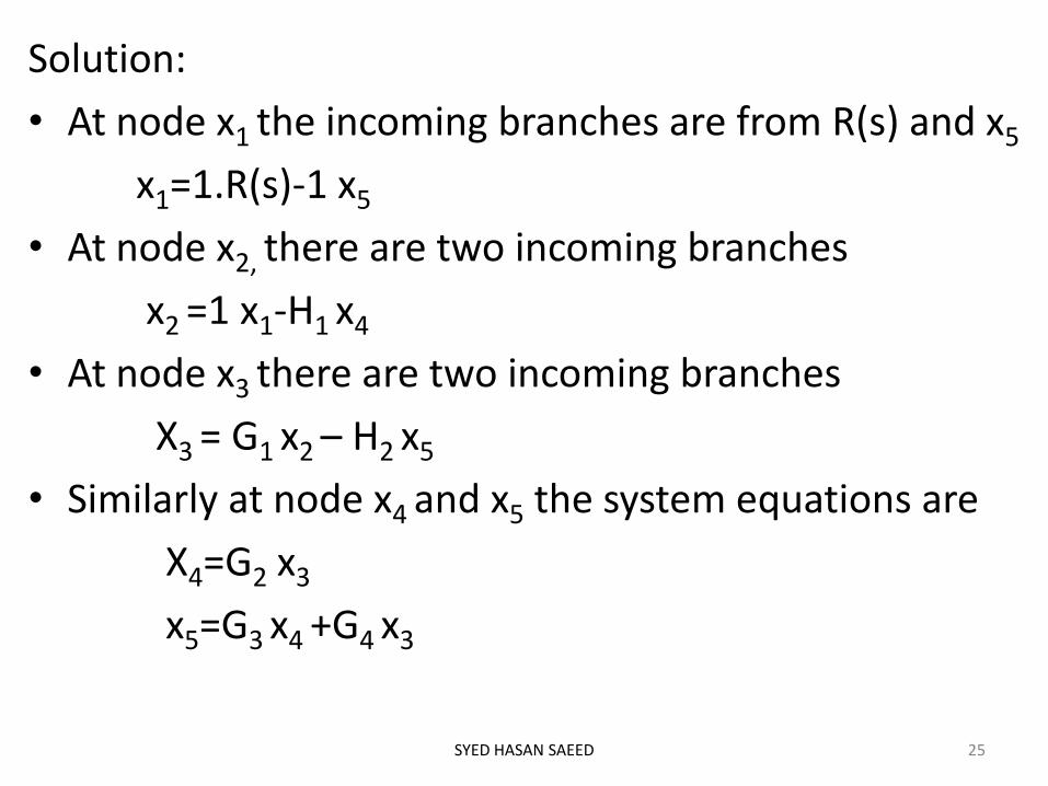
Solution:

• At node x1 the incoming branches are from R(s) and x5

x1=1.R(s)-1 x5

• At node x2, there are two incoming branches

x2 =1 x1-H1 x4

• At node x3 there are two incoming branches

X3 = G1 x2 – H2 x5

• Similarly at node x4 and x5 the system equations are

X4=G2 x3

x5=G3 x4 +G4 x3

SYED HASAN SAEED 25

Draw the block diagram for x1=1.R(s)-1 x5

R(s) + x1

x5

Block diagram for x2 = x1-H1 x4

x1 + x2

x4 4

SYED HASAN SAEED 26

1

1

H1

1

Block diagram for x3 = G1 x2 – H2 x5

x2 + x3

x5

Block diagram for x4=G2 x3

x3 G2 x4

SYED HASAN SAEED 27

G1

H2

Block diagram for x5=G3 x4 +G4 x3

x4 + x5

+

x3

SYED HASAN SAEED 28

G3

G4

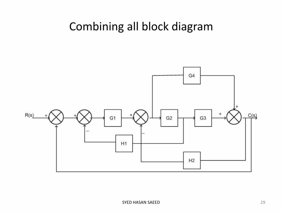
Combining all block diagram

SYED HASAN SAEED 29

EFFECT OF FEEDBACK ON OVERALL GAIN

R(s) C(s)

The overall transfer function of open loop system is

The overall transfer function of closed loop system is

For negative feedback the gain G(s) is reduced by a factor

So due to negative feedback overall gain of the system is reduced

SYED HASAN SAEED 30

G(s)

)()(

)(sG

sR

sC

)()(1

)(

)(

)(

sHsG

sG

sR

sC

)()(1

1

sHsG

EFFECT OF FEEDBACK ON STABILITY

SYED HASAN SAEED 31

Consider the open loop system with overall transfer function

The pole is located at s=-T

Now, consider closed loop system with unity negative feedback, then overall transfer function is given by

Now closed loop pole is located at s=-(T+K) Thus, feedback controls the time response by adjusting the

location of poles. The stability depends upon the location of the poles. Thus feedback affects the stability.

Ts

KsG

)(

)()(

)(

KTs

K

sR

sC

OUTLINE

Definition of Transfer Function.

Poles & Zeros.

Characteristic Equation.

Advantages of Transfer Function.

Mechanical System (i) Translational System and (ii) Rotational System.

Free Body diagram.

Transfer Function of Electrical, Mechanical Systems.

D’Alembert Principle.

SYED HASAN SAEED

TRANSFER FUNCTION

Definition: The transfer function is defined as the ratio of Laplace transform of the output to the Laplace transform of input with all initial conditions are zero.

We can defined the transfer function as

SYED HASAN SAEED 2

)0.1(.....

.....)(

)(

)(

01

1

1

01

1

1

asasasa

bsbsbsbsG

sR

sCn

n

n

n

m

m

m

m

In equation (1.0), if the order of the denominator polynomial is greater than the order of the numerator polynomial then the transfer function is said to be STRICTLY PROPER. If the order of both polynomials are same, then the transfer function is PROPER. The transfer function is said to be IMPROPER, if the order of numerator polynomial is greater than the order of the denominator polynomial.

CHARACTERISTIC EQUATION: The characteristic equation can be obtained by equating the denominator polynomial of the transfer function to zero. That is

SYED HASAN SAEED 3

0..... 01

1

1

asasasa n

n

n

n

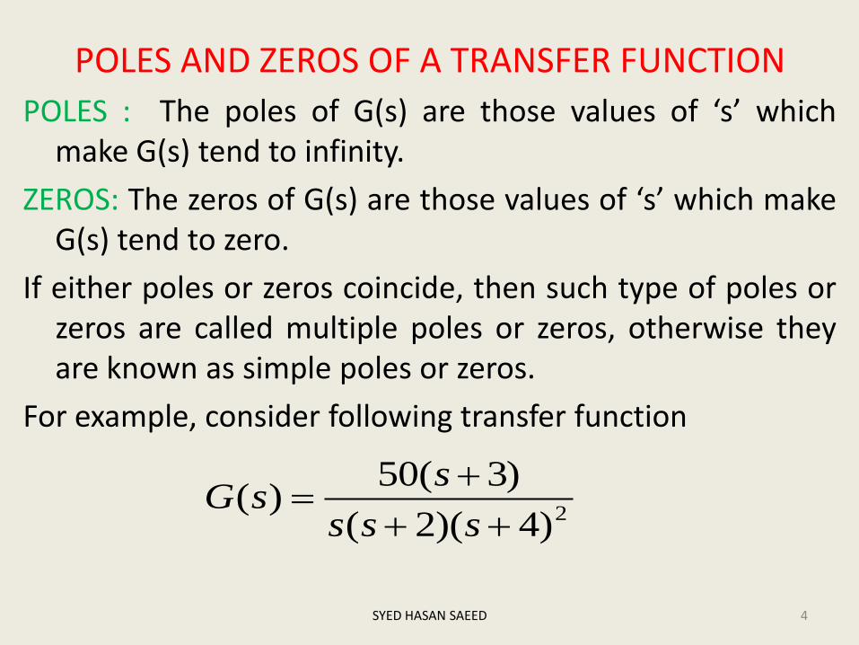
POLES AND ZEROS OF A TRANSFER FUNCTION

POLES : The poles of G(s) are those values of ‘s’ which make G(s) tend to infinity.

ZEROS: The zeros of G(s) are those values of ‘s’ which make G(s) tend to zero.

If either poles or zeros coincide, then such type of poles or zeros are called multiple poles or zeros, otherwise they are known as simple poles or zeros.

For example, consider following transfer function

SYED HASAN SAEED 4

2)4)(2(

)3(50)(

sss

ssG

This transfer function having the simple poles at s=0, s=-2, multiple poles at s=-4 and simple zero at s=-3.

Advantages of Transfer Function:

1. Transfer function is a mathematical model of all system components and hence of the overall system and therefore it gives the gain of the system.

2. Since Laplace transform is used, it converts time domain equations to simple algebraic equations.

3. With the help of transfer function, poles, zeros and characteristic equation can be determine.

4. The differential equation of the system can be obtained by replacing ‘s’ with d/dt.

SYED HASAN SAEED 5

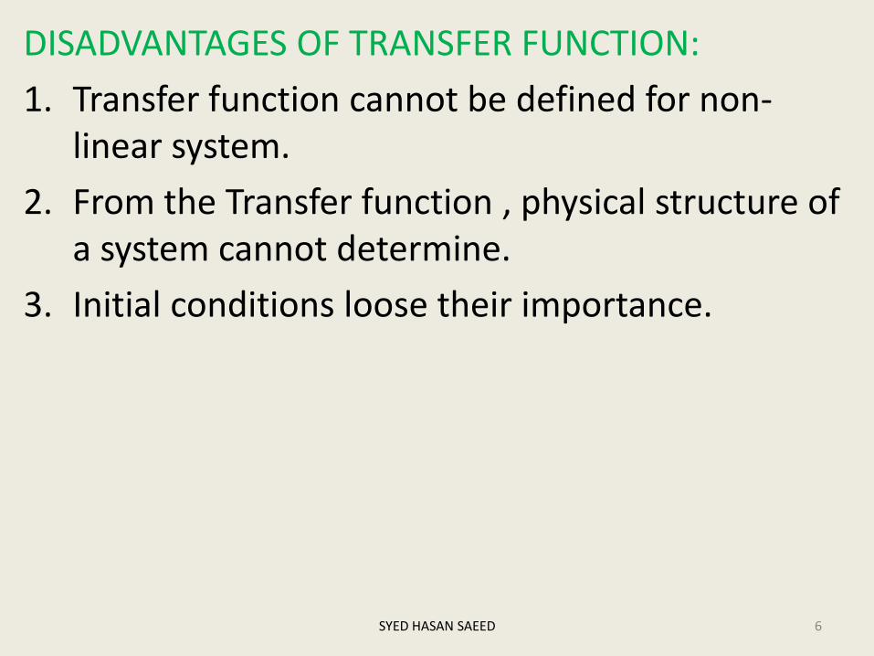
DISADVANTAGES OF TRANSFER FUNCTION:

1. Transfer function cannot be defined for non-linear system.

2. From the Transfer function , physical structure of a system cannot determine.

3. Initial conditions loose their importance.

SYED HASAN SAEED 6

Find the transfer function of the given figure.

Solution:

Step 1: Apply KVL in mesh 1 and mesh 2

SYED HASAN SAEED 7

)2(

)1(

dt

diLv

dt

diLRiv

o

i

Step 2: take Laplace transform of eq. (1) and (2)

Step 3: calculation of transfer function

Equation (5) is the required transfer function

SYED HASAN SAEED 8

)4()()(

)3()()()(

ssLIsV

ssLIsRIsV

o

i

)5()(

)(

)()(

)(

)(

)(

sLR

sL

sV

sV

sIsLR

ssLI

sV

sV

i

o

i

o

A system having input x(t) and output y(t) is represented by

Equation (1). Find the transfer function of the system.

Solution: taking Laplace transform of equation (1)

G(s) is the required transfer function

SYED HASAN SAEED

)1()(5)(

)(4)(

txdt

tdxty

dt

tdy

4

5

)(

)()(

4

5

)(

)(

)5)(()4)((

)(5)()(4)(

s

s

sX

sYsG

s

s

sX

sY

ssXssY

sXssXsYssY

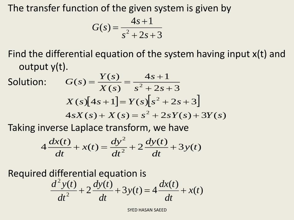
The transfer function of the given system is given by

Find the differential equation of the system having input x(t) and output y(t).

Solution:

Taking inverse Laplace transform, we have

Required differential equation is

SYED HASAN SAEED

32

14)(

2

ss

ssG

)(3)(2)()(4

32)(14)(

32

14

)(

)()(

2

2

2

sYssYssXssX

sssYssX

ss

s

sX

sYsG

)(3)(

2)()(

42

2

tydt

tdy

dt

dytx

dt

tdx

)()(

4)(3)(

2)(

2

2

txdt

tdxty

dt

tdy

dt

tyd

MECHANICAL SYSTEM

TRANSLATIONAL SYSTEM: The motion takes place along a strong line is known as translational motion. There are three types of forces that resists motion.

INERTIA FORCE: consider a body of mass ‘M’ and acceleration ‘a’, then according to Newton’s law of motion

FM(t)=Ma(t)

If v(t) is the velocity and x(t) is the displacement then

dt

tdvMtFM

)()(

2

2 )(

dt

txdM

SYED HASAN SAEED

M

)(tx

)(tF

DAMPING FORCE: For viscous friction we assume that the damping force is proportional to the velocity.

FD(t)=B v(t)

Where B= Damping Coefficient in N/m/sec.

We can represent ‘B’ by a dashpot consists of piston and cylinder.

SYED HASAN SAEED

dt

tdxB

)(

)(tFD

)(tx

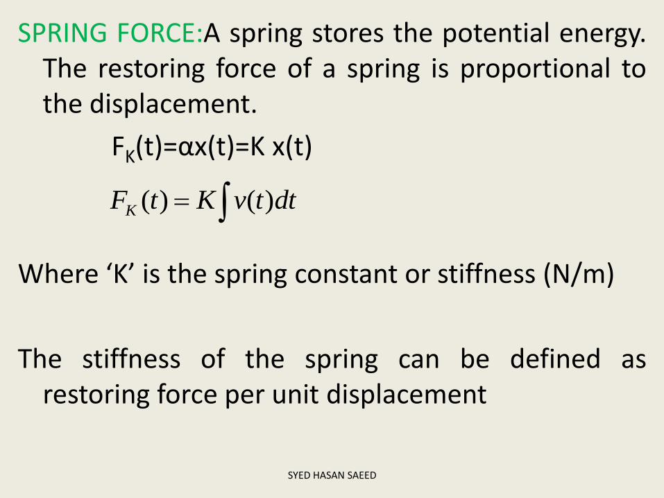
SPRING FORCE:A spring stores the potential energy. The restoring force of a spring is proportional to the displacement.

FK(t)=αx(t)=K x(t)

Where ‘K’ is the spring constant or stiffness (N/m)

The stiffness of the spring can be defined as restoring force per unit displacement

SYED HASAN SAEED

dttvKtFK )()(

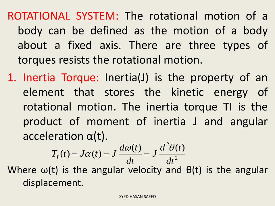
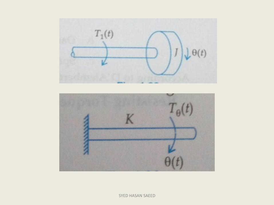
ROTATIONAL SYSTEM: The rotational motion of a body can be defined as the motion of a body about a fixed axis. There are three types of torques resists the rotational motion.

1. Inertia Torque: Inertia(J) is the property of an element that stores the kinetic energy of rotational motion. The inertia torque TI is the product of moment of inertia J and angular acceleration α(t).

Where ω(t) is the angular velocity and θ(t) is the angular displacement.

SYED HASAN SAEED

2

2 )()()()(

dt

tdJ

dt

tdJtJtTI

SYED HASAN SAEED

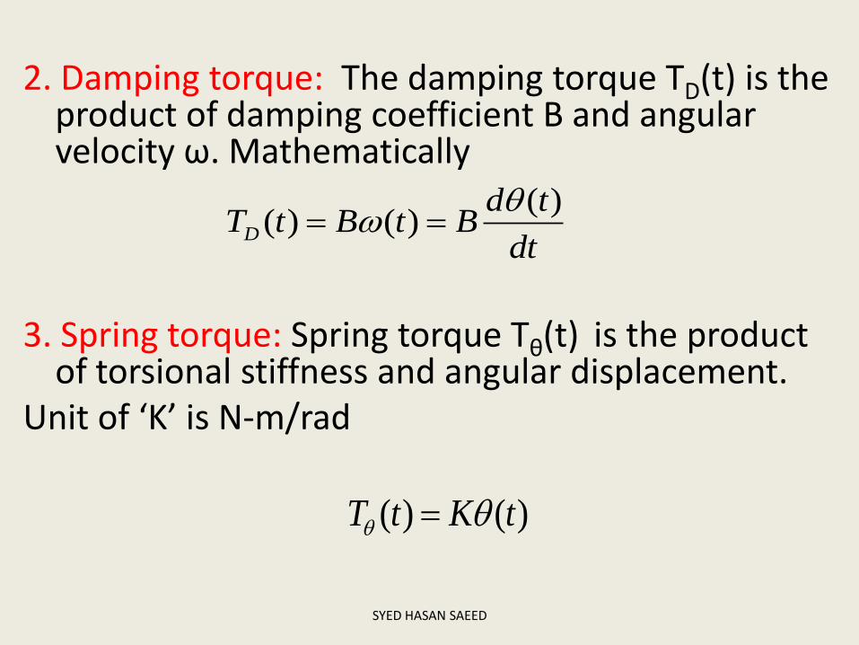
2. Damping torque: The damping torque TD(t) is the product of damping coefficient B and angular velocity ω. Mathematically

3. Spring torque: Spring torque Tθ(t) is the product

of torsional stiffness and angular displacement. Unit of ‘K’ is N-m/rad SYED HASAN SAEED

dt

tdBtBtTD

)()()(

)()( tKtT

D’ALEMBERT PRINCIPLE

This principle states that “for any body, the algebraic sum of externally applied forces and the forces resisting motion in any given direction is zero”

SYED HASAN SAEED

D’ALEMBERT PRINCIPLE contd……

External Force: F(t)

Resisting Forces :

1. Inertia Force:

2. Damping Force:

3. Spring Force:

SYED HASAN SAEED

2

2 )()(

dt

txdMtFM

dt

tdxBtFD

)()(

)()( tKxtFK

M

F(t)

X(t)

According to D’Alembert Principle

SYED HASAN SAEED

0)()()(

)(2

2

tKxdt

tdxB

dt

txdMtF

)()()(

)(2

2

tKxdt

tdxB

dt

txdMtF

Consider rotational system:

External torque: T(t)

Resisting Torque:

(i) Inertia Torque:

(ii) Damping Torque:

(iii) Spring Torque:

According to D’Alembert Principle:

SYED HASAN SAEED

dt

tdJtTI

)()(

dt

tdBtTD

)()(

)()( tKtTK

0)()()()( tTtTtTtT KDI

SYED HASAN SAEED

0)()()(

)( tKdt

tdB

dt

tdJtT

)()()(

)( tKdt

tdB

dt

tdJtT

D'Alembert Principle for rotational motion states that “For anybody, the algebraic sum of externally applied torques and the torque resisting rotation about any axis is zero.”

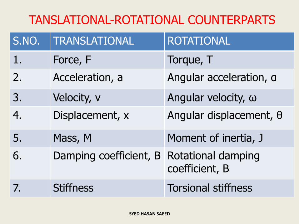
TANSLATIONAL-ROTATIONAL COUNTERPARTS

S.NO. TRANSLATIONAL ROTATIONAL

1. Force, F Torque, T

2. Acceleration, a Angular acceleration, α

3. Velocity, v Angular velocity, ω

4. Displacement, x Angular displacement, θ

5. Mass, M Moment of inertia, J

6. Damping coefficient, B Rotational damping coefficient, B

7. Stiffness Torsional stiffness

SYED HASAN SAEED

EXAMPLE: Draw the free body diagram and write the differential equation of the given system shown in fig.

Solution:

Free body diagrams are shown in next slide

SYED HASAN SAEED

SYED HASAN SAEED

2

1

2

1dt

xdM

)( 211 xxK dt

xxdB

)( 211

)(tF

1M 2M

)( 211 xxK dt

xxdB

)( 211

2

2

2

2dt

xdM

dt

dxB 2

2 22xK

222

22

2

2

221

1211

21121

12

1

2

1

211

211

2

1

2

1

)()(

)()(

)(

)(

)(

xKdt

dxB

dt

xdM

dt

xxdBxxK

similarly

xxKdt

xxdB

dt

xdMtF

xxKF

dt

xxdBF

dt

xdMF

K

D

M

SYED HASAN SAEED

Figure

Write the differential equations describing the dynamics of the systems shown in figure and find the ratio

SYED HASAN SAEED

)(

)(2

sF

sX

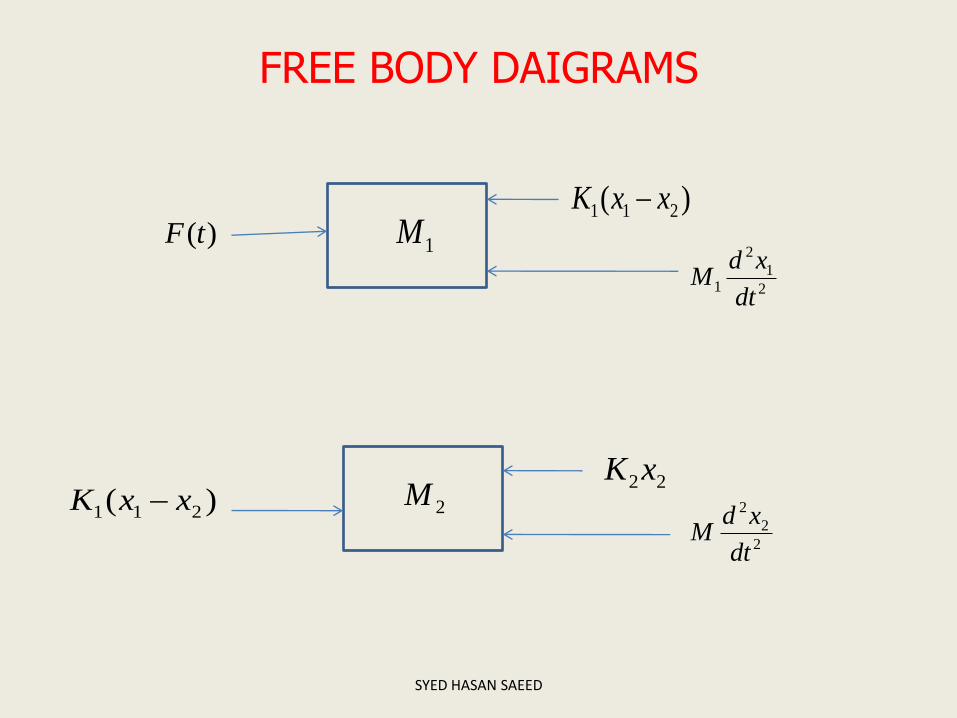
FREE BODY DAIGRAMS

SYED HASAN SAEED

1M

2

1

2

1dt

xdM

)( 211 xxK )(tF

2M

2

2

2

dt

xdM

22xK)( 211 xxK

Differential equations are

SYED HASAN SAEED

2

2

2

222211

2112

1

2

1

)(

)()(

dt

xdMxKxxK

xxKdt

xdMtF

LaplaceTransform of above equations

)()()()(

)()()()(

2

2

2222111

21111

2

1

sXsMsXKsXKsXK

sXKsXKsXsMsF

Solve equationsabove for

2

11

2

1212

2

12

))(()(

)(

KMsKKKMs

K

sF

sX

)(

)(2

sF

sX

THANK YOU

SYED HASAN SAEED