Outline 2.1 Graph Isomorphism 2.2 Automorphisms and Symmetry …cs4203/files/GT-Lec2.pdf · ·...

GRAPH THEORY – LECTURE 2STRUCTURE AND REPRESENTATION — PART A

Abstract. Chapter 2 focuses on the question of when two graphs are to be regarded as “the same”, onsymmetries, and on subgraphs. §2.1 discusses the concept of graph isomorphism. §2.2 presents symmetryfrom the perspective of automorphisms. §2.3 introduces subgraphs.

Outline

2.1 Graph Isomorphism2.2 Automorphisms and Symmetry2.3 Subgraphs, part 1

1

2 GRAPH THEORY – LECTURE 2 STRUCTURE AND REPRESENTATION — PART A

1. Graph Isomorphism

0

2

1

3

6 7

541

0

2 3

7

4

6

5

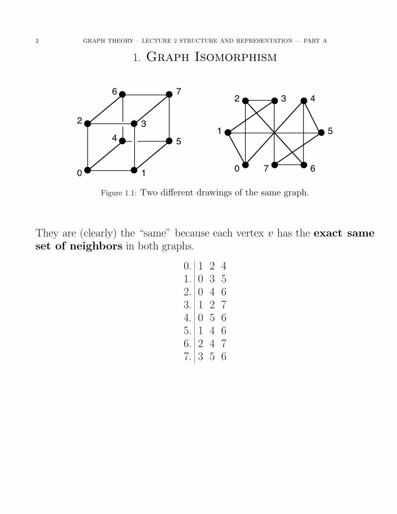
Figure 1.1: Two different drawings of the same graph.

They are (clearly) the “same” because each vertex v has the exact sameset of neighbors in both graphs.

0. 1 2 41. 0 3 52. 0 4 63. 1 2 74. 0 5 65. 1 4 66. 2 4 77. 3 5 6

GRAPH THEORY – LECTURE 2 STRUCTURE AND REPRESENTATION — PART A 3

1

4

6

7

2

3

5

8

s

t

u

vw

x

yz

G H

Figure 1.2: Two more drawings of that same graph.

These two graphs are the “same” because, instead of having the same setof vertices, this time we have a bijection VG → VH

1→ s 2→ t 3→ u 4→ v5→ w 6→ x 7→ y 8→ z

between the two vertex sets, such that

Nbhds map bijectively to nbhds;

e.g., N(1) 7→ N(f (1)) = N(s), i.e.

N(1) = {2, 3, 5} 7→ {t, u, w} = {f (2), f (3), f (5)} = N(s)


Structural Equivalence for Simple Graphs

Def 1.1. LetG andH be two simple graphs. A vertex function f : VG → VHpreserves adjacency if

for every pair of adjacent vertices u and v in graph G,the vertices f (u) and f (v) are adjacent in graph H .

Similarly, f preserves non-adjacency if

f (u) and f (v) are non-adj whenever u and v are non-adj.

Def 1.2. A vertex bijection f : VG → VH betw. two simple graphs G andH is structure-preserving if

it preserves adjacency and non-adjacency.

That is, for every pair of vertices in G,

u and v are adj in G ⇐⇒ f (u) and f (v) are adj in H

This leads us to a formal mathematical definition of what we mean by the“same” graph.


Def 1.3. Two simple graphs G and H are isomorphic, denoted G ∼= H ,if

∃ a structure-preserving bijection f : VG → VH .

Such a function f is called an isomorphism from G to H .

Notation: When we regard a vertex function f : VG → VH as a mappingfrom one graph to another, we may write f : G→ H .

ISOMORPHISM CONCEPT

Two graphs related by isomorphism differ only bythe names of the vertices and edges. There is acomplete structural equivalence between two suchgraphs.


REPRESENTATION by DRAWINGS

When the drawings of two isomorphic graphs lookdifferent, relabeling reveals the equivalence.

One may use functional notation to specify an isomorphism between the twosimple graphs shown.

a=f(0)

d=f(3)

f=f(5)

g=f(6)

b=f(1)

c=f(2)

e=f(4)

h=f(7)0

2

1

3

6 7

54

Figure 1.3: Specifying an isom betw two simple graphs.

Alternatively, one may relabel the vertices of the codomain graph with namesof vertices in the domain, as in Fig 1.4.

0

3

5

6

1

2

4

70

2

1

3

6 7

54

Figure 1.4: Another way of depicting an isomorphism.


ISOMORPHISM (SIMPLE) =

BIJECTIVE on VERTICESADJACENCY-PRESERVING

(NON-ADJACENCY)-PRESERVING

Example 1.1. The vertex function j 7→ j+4 depicted in Fig 1.5 is bijectiveand adjacency-preserving, but it is not an isomorphism, since it does notpreserve non-adjacency.

In particular, the non-adjacent pair {0, 2} maps to the adjacent pair {4, 6}.

0

1 2

3 4

5 6

7

Figure 1.5: Bijective and adj-preserving, but not an isom.


Example 1.2. The vertex function

j 7→ j mod 2

depicted in Figure 1.6 is structure-preserving, since it preserves adja-cency and non-adjacency, but it is not an isomorphism since it is notbijective.

Figure 1.6: Preserves adj and non-adj, but not bijective.


Isomorphism for General Graphs

The mapping f : VG → VH between the vertex-sets of the two graphs shownin Figure 1.7 given by

f (i) = i, i = 1, 2, 3

preserves adjacency and non-adjacency, but the two graphs are clearly notstructurally equivalent.

21

3

21

3

Figure 1.7: These graphs are not structurally equivalent.

Def 1.4. A vertex bijection f : VG → VH between two graphs G and H ,simple or general, is structure-preserving if

(1) the # of edges (even if 0) between every pair of distinct verticesu and v in graph G equals the # of edges between their imagesf (u) and f (v) in graph H , and

(2) the # of self-loops at each vertex x in G equals the # ofself-loops at the vertex f (x) in H .


21

3

21

3

This general definition of structure-preserving reduces, for simple graphs, toour original definition. Moreover, it allows a unified definition of isomorphicgraphs for all cases.

Def 1.5. Two graphsG andH (simple or general) are isomorphic graphsif ∃ structure-preserving vertex bijection f : VG → VH

This relationship is denoted G ∼= H .


Isomorphism for Graphs with Multi-Edges

Def 1.6. For isomorphic graphs G and H , a pair of bijections

fV : VG → VH and fE : EG → EH

is consistent if for every edge e ∈ EG, the function fV maps the endpointsof e to the endpoints of the edge fE(e).

Proposition 1.1. G ∼= H iff there is a consistent pair of bijections

fV : VG → VH and fE : EG → EH

Proof. Straightforward from the definitions. �

Remark 1.1. If G and H are isom simple graphs, then every structure-preserving vertex bijection f : VG → VH induces a unique consistent edgebijection, by the rule: uv 7→ f (u)f (v).


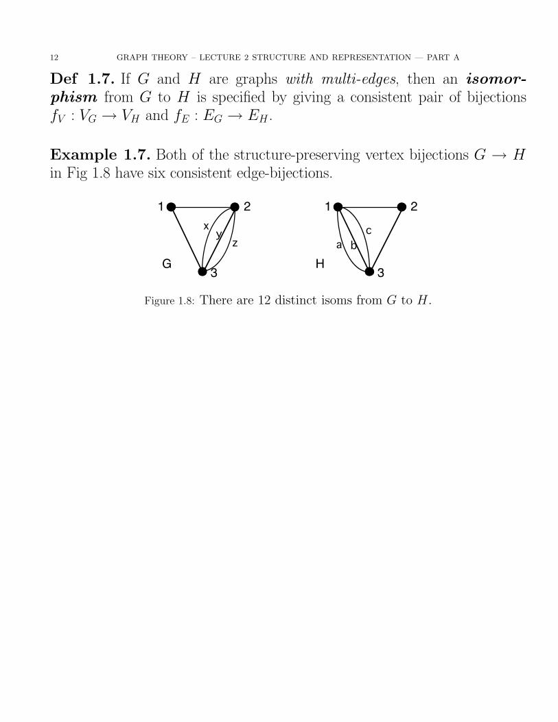
Def 1.7. If G and H are graphs with multi-edges, then an isomor-phism from G to H is specified by giving a consistent pair of bijectionsfV : VG → VH and fE : EG → EH .

Example 1.7. Both of the structure-preserving vertex bijections G → Hin Fig 1.8 have six consistent edge-bijections.

21

3

21

3

a bcx y

z

G H

Figure 1.8: There are 12 distinct isoms from G to H.


Necessary Properties of Isom Graph Pairs

Although the examples below involve simple graphs, the properties apply togeneral graphs as well.

Theorem 1.2. Let G and H be isomorphic graphs. Then they have thesame number of vertices and edges.

Proof. An isomorphism maps VG and EG bijectively. �

Theorem 1.3. Let f : G→ H be a graph isomorphism and let v ∈ VG.Then deg(f (v)) = deg(v).

Proof. Since f is structure-preserving, the # of proper edges and the # ofself-loops incident on vertex v equal the corresp #’s for vertex f (v). Thus,deg(f (v)) = deg(v). �

Corollary 1.4. Let G and H be isomorphic graphs. Then they have thesame degree sequence.

Corollary 1.5. Let f : G→ H be a graph isom and e ∈ EG. Then theendpoints of edge f (e) have the same degrees as the endpoints of e.


Example 1.8. In Fig 1.9 below, we observe that Q3 and CL4 both have 8vertices and 12 edges and are 3-regular.

The vertex labelings specify a vertex bijection. A careful examination revealsthat this vertex bijection is structure-preserving.

It follows that Q3 and CL4 are isomorphic graphs.

000 001

011

111110

100101

010

f(010)

f(000)

f(001)

f(011)f(100)

f(101)

f(111)

f(110)

Figure 1.9: Hypercube Q3 and circ ladder CL4 are isom.


Def 1.8. The Mobius ladder MLn is a graph obtained from the circularladder CLn by deleting from the circular ladder two of its parallel curvededges and replacing them with two edges that cross-match their endpoints.

Example 1.9. K3,3 and the Mobius ladder ML3 both have 6 vertices and9 edges, and both are 3-regular.

The vertex labelings for the two drawings specify an isomorphism.

0 2 4

1 3 5

0

1

2

3

4

5

ML3 K3,3

Figure 1.10: K3,3 and the Mobius ladder ML3 are isom.


Isomorphism Type of a Graph

Def 1.9. Each equivalence class under ∼= is called an isomorphism type.(Counting isomorphism types of graphs generally involves the algebra ofpermutation groups — see Chap 14).

Figure 1.11: The 4 isom types for a simple 3-vertex graph.


Isomorphism of Digraphs

Def 1.10. Two digraphs G and H are isomorphic if there is an isomor-phism f between their underlying graphs that preserves the direction of eachedge.

Example 1.10. Notice that non-isomorphic digraphs can have underlyinggraphs that are isomorphic.

Figure 1.12: Four non-isomorphic digraphs.

Def 1.11. The graph-isomorphism problem is to devisea practical general algorithm to decide graph isomorphism, or,alternatively, to prove that no such algorithm exists.


2. Automorphisms & Symmetry

Def 2.1. An isomorphism from a graph G to itself is called an automor-phism.

Thus, an automorphism π of graphG is a structure-preserving permutation

πV on VG

along with a (consistent) permutation

πE on EG

We may write π = (πV , πE).

Remark 2.1. The proportion of vertex-permutations of VG that are structure-preserving is a measure of the symmetry of G.


Permutations and Cycle Notation

The most convenient representation of a permutation, for our present pur-poses, is as a product of disjoint cycles.

Remark 2.2. As explained in Appendix A4, every permutation can bewritten as a composition of disjoint cycles.

Example 2.1. The permutation

π =

(1 2 3 4 5 6 7 8 97 4 1 8 5 2 9 6 3

)which maps 1 to 7, 2 to 4, and so on, has the disjoint cycle form

π =(1 7 9 3

) (2 4 8 6

) (5)


Geometric Symmetry

A geometric symmetry on a graph drawing can be used to represent anautomorphism on the graph.

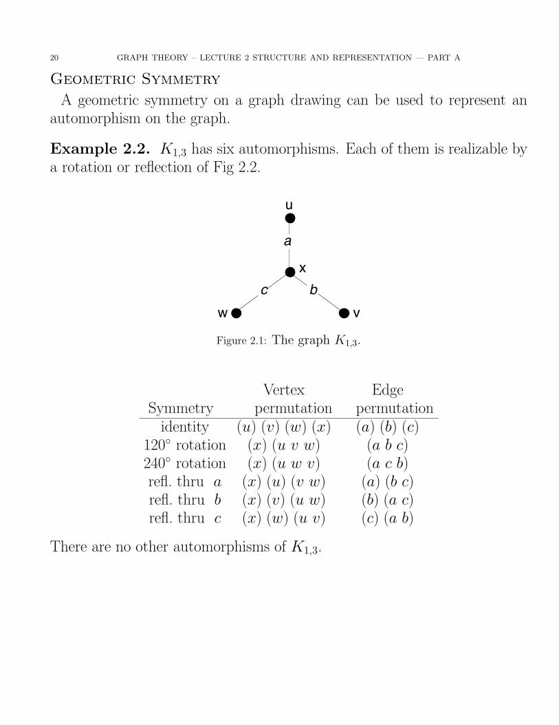
Example 2.2. K1,3 has six automorphisms. Each of them is realizable bya rotation or reflection of Fig 2.2.

x

w

u

v

a

bc

Figure 2.1: The graph K1,3.

Vertex EdgeSymmetry permutation permutation

identity (u) (v) (w) (x) (a) (b) (c)120◦ rotation (x) (u v w) (a b c)240◦ rotation (x) (u w v) (a c b)refl. thru a (x) (u) (v w) (a) (b c)refl. thru b (x) (v) (u w) (b) (a c)refl. thru c (x) (w) (u v) (c) (a b)

There are no other automorphisms of K1,3.


Example 2.3. It is easy to verify that these vertex-perms are structure-preserving, so they are all graph automorphisms.

1 23

4

5

6

7 8

Automorphismsλ0 = 1( ) 2( ) 3( ) 4( ) 5( ) 6( ) 7( ) 8( )

λ1= 1 8( ) 2 7( ) 3( ) 4( ) 5( ) 6( )

λ2 = 1( ) 2( ) 3 5( ) 4 6( ) 7( ) 8( )

λ3= 1 8( ) 2 7( ) 3 5( ) 4 6( )

Figure 2.2: A graph with four automorphisms.


Limitations of Geometric Symmetry

Example 2.4. The leftmost drawing has 5-fold rotational symmetry thatcorresponds to the automorphism (0 1 2 3 4) (5 6 7 8 9), but this automor-phism does not correspond to any geometric symmetry of either of the othertwo drawings.

0

1

23

456

78

9

0 5

7

23

4

9

8 16 6

1

8 9

0

4

75

2

3

(a) (b) (c)

Figure 2.3: Three drawings of the Petersen graph.


Vertex- and Edge-Transitive Graphs

Def 2.2. A graph G is vertex-transitive if for every vertex pair u, v ∈VG, there is an automorphism that maps u to v.

Def 2.3. A graph G is edge-transitive if for every edge pair d, e ∈ EG,there is an automorphism that maps d to e.

Example 2.5. K1,3 is edge-trans, but not vertex-trans, since every autommust map the 3-valent vertex to itself.

Example 2.7. The hypercube graph Qn is vertex-trans and edge-trans forevery n. (See Exercises.)

Example 2.8. Every circulant graph circ(n;S) is vertex-transitive. Inparticular, the vertex function i 7→ i + k mod n is an automorphism. Al-though circ(13 : 1, 5) is edge-transitive, some circulant graphs are not. (SeeExercises.)

0 1

2

3

4

567

8

9

10

11

12

Figure 2.4: The circulant graph circ(13 : 1, 5).


Vertex Orbits and Edge Orbits

Def 2.4. The equivalence classes of the vertices of a graph G under theaction of the automorphisms are called vertex orbits. The equivalenceclasses of the edges are called edge orbits.

Example 2.10.

vertex orbits: {1,8}, {4,6}, {2,7}, {3,5}edge orbits: {12,78}, {34,56}, {23,25,37,57}, {35}

1 23

4

5

6

7 8

Automorphismsλ0 = 1( ) 2( ) 3( ) 4( ) 5( ) 6( ) 7( ) 8( )

λ1= 1 8( ) 2 7( ) 3( ) 4( ) 5( ) 6( )

λ2 = 1( ) 2( ) 3 5( ) 4 6( ) 7( ) 8( )

λ3= 1 8( ) 2 7( ) 3 5( ) 4 6( )

Figure 2.5: Graph of Example 2.3.


Theorem 2.1. All vertices in the same orbit have the exact same degree.

Proof. This follows immediately from Theorem 1.3. �

Theorem 2.2. All edges in the same orbit have the same pair of degreesat their endpoints.

Proof. This follows immediately from Corollary 1.5. �

Example 2.11. Each of the two partite sets of Km,n is a vertex orbit. Thegraph is vertex-transitive if and only if m = n; otherwise it has two vertexorbits. However, Km,n is always edge-transitive (see Exercises).


How to Find the Orbits

We illustrate how to find orbits by consideration of two examples. (Itis not known whether there exists a polynomial-time algorithm for findingorbits. Testing all n! vertex-perms for the adjacency preservation propertyis too tedious an approach.) In addition to using Theorems 2.1 and 2.2, weobserve that if an automorphism maps vertex u to vertex v, then it mapsthe neighbors of u to the neighbors of v.

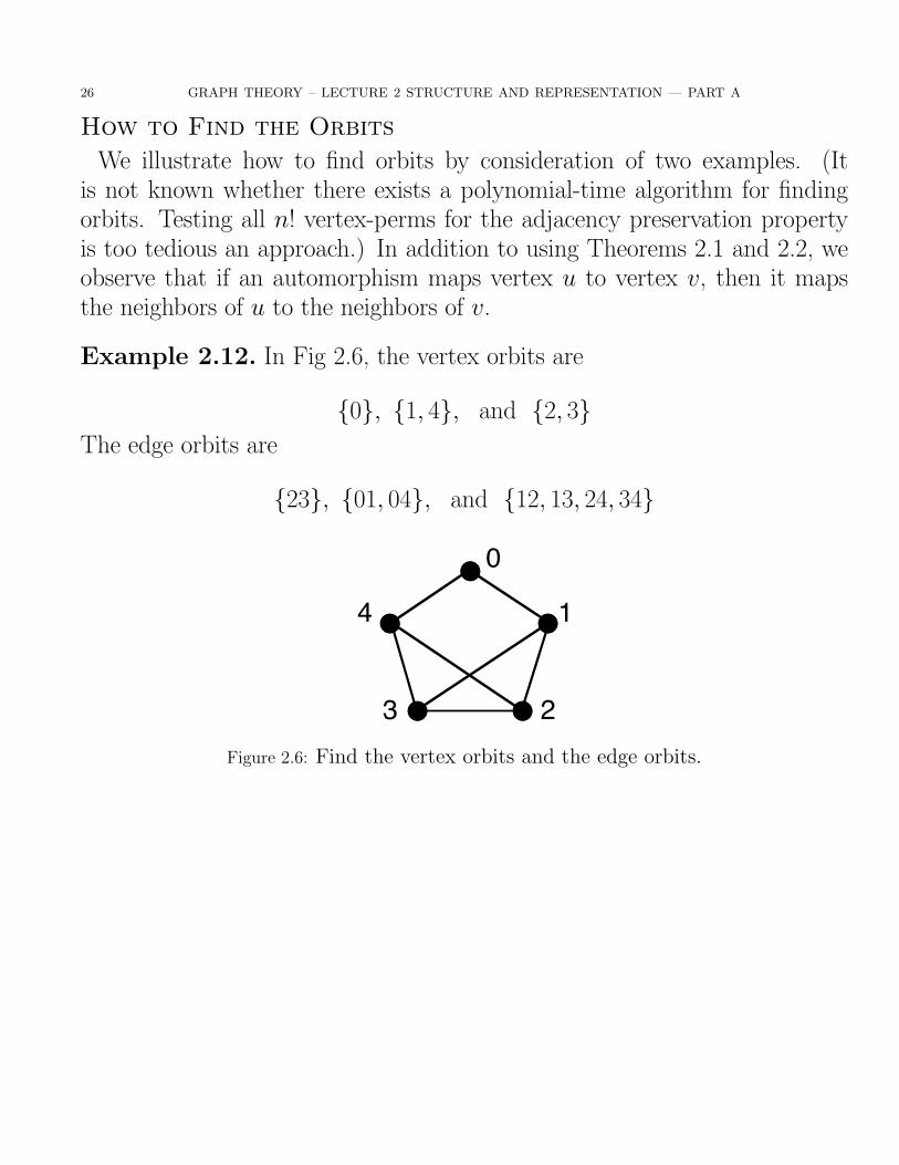
Example 2.12. In Fig 2.6, the vertex orbits are

{0}, {1, 4}, and {2, 3}The edge orbits are

{23}, {01, 04}, and {12, 13, 24, 34}

0

1

3

4

2Figure 2.6: Find the vertex orbits and the edge orbits.


Example 2.13. We could approach the 4-regular graph of Figure 2.7 byrecognizing the symmetry (0 5)(1 4)(2)(3)(6) and seeking to find others.However, it is possible to expedite the determination of orbits.

0 1

3

4

2

5

6

Figure 2.7: Find the vertex orbits and the edge orbits.

When we look at vertices 0, 2, 3, and 5, we discover that each of them has aset of 3 neighbors that are independent, while vertices 1, 4, and 6 each havetwo pairs of adjacent vertices. This motivates us to redraw the graph as inFigure 2.8.

0

1

3

4

25

6

Figure 2.8: Find the vertex orbits and the edge orbits.

In that form, we see immediately that there are two vertex orbits, namely{0, 2, 3, 5} and {1, 4, 6}. One of the two edge orbits is {05, 23}, and theother contains all the other edges.


3. Subgraphs

Def 3.1. A subgraph of a graph G is a graph H whose vertices and edgesare all in G. If H is subgraph of G, we may also say that G is a supergraphof H .

Def 3.2. A proper subgraph H of G is a subgraph such that VH is aproper subset of VG or EH is a proper subset of EG.

Example 3.1. Fig 3.1 shows the line drawings and corresponding incidencetables for two proper subgraphs of a graph.

u v

x

w z

a

bc

d

e

u v

x

w z

a

bcd

ef

G

u v

x

cd

a b c d e f

u v v u x wv z x x w z

edge

endpts

edge

endpts

c d

v ux x

edge a b c d e

u v v u xv z x x w

endpts

H1

H2

Figure 3.1: A graph G and two (proper) subgraphs H1 and H2.

The usual meaning of the phrase “H is a subgraph of G” is that H is merelyisomorphic to a subgraph of G.


Spanning Subgraphs

Def 3.3. A subgraph H is said to span a graph G if VH = VG.

Def 3.4. A spanning tree is a spanning subgraph that is a tree.

Figure 3.3: A spanning tree.

Def 3.5. An acyclic graph is called a forest.

G

Figure 3.4: A spanning forest H of graph G.


Cliques and Independent Sets

Def 3.6. A subset S of VG is called a clique if every pair of vertices in Sis joined by at least one edge, and no proper superset of S has this property.

Def 3.7. The clique number of a graph G is the number ω(G) of verticesin a largest clique in G.

Example 3.2. In Fig 3.5, the vertex subsets, {u, v, y}, {u, x, y}, and {y, z}induce complete subgraphs, and ω(G) = 3.

u v

x y z

Figure 3.5: A graph with three cliques.

Def 3.8. A subset S of VG is said to be an independent set if no pairof vertices in S is joined by an edge.

Def 3.9. The independence number of a graph G is the number α(G)of vertices in a largest independent set in G.

Remark 3.1. Thus, the clique # ω(G) and the indep # α(G) are comple-mentary concepts (in the sense described in §2.4).


Induced Subgraphs

Def 3.10. Subgraph induced on subset U of VG, denoted G(U).

VG(U) = U and EG(U) = {e ∈ EG : endpts(e) ⊆ U}

u

v

w

a b

c

d

hf

g

induced on {u, v}

u

v

w

a b

c

d

hf

g

Figure 3.6: A subgraph induced on a subset of vertices.


7. Supplementary Exercises

Exercise 1 Draw all isomorphism types of general graphs with 2 edgesand no isolated vertices.

Exercise 14 List the vertex orbits and the edge orbits of the graph ofFig 7.1.

0 1

23 4

56 7

8 9

Figure 7.1:

Exercise 17 Some of the 4-vertex, simple graphs have exactly two vertexorbits. Draw an illustration of each such isomorphism type.

Outline 2.1 Graph Isomorphism 2.2 Automorphisms and Symmetry …cs4203/files/GT-Lec2.pdf · ·...

Documents

Transcript of Outline 2.1 Graph Isomorphism 2.2 Automorphisms and Symmetry …cs4203/files/GT-Lec2.pdf · ·...