Outdoor path loss models for ieee 802.16

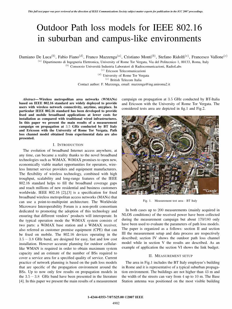
Outdoor Path loss models for IEEE 802.16in suburban and campus-like environments

Damiano De Luca(b), Fabio Fiano(d), Franco Mazzenga(a), Cristiano Monti(b), Stefano Ridolfi(e), Francesco Vallone(c)

(a) Dipartimento di Ingegneria Elettronica, University of Rome Tor Vergata, Via del Politecnico 1, 00133, Roma, Italy(b) Consorzio Universita Industria Laboratori di Radiocomunicazioni, RadioLabs

(c) Ericsson Telecomunicazioni(d) University of Rome Tor Vergata

(e) British Telecom ItaliaContact author: F. Mazzenga, email: [email protected]

Abstract— Wireless metropolitan area networks (WMANs)based on IEEE 802.16 standard are widely deployed to provideusers with wireless network connectivity, anytime, anyplace. Inparticular IEEE 802.16 standard has been developed to providefixed and mobile broadband applications at lower costs forinstallation as compared with traditional wired infrastructures.In this paper we present the main results of a measurementcampaign on propagation at 3.5 GHz conducted by BT Italyand Ericsson with the University of Rome Tor Vergata. Pathloss channel model obtained from experimental data are alsopresented.

I. INTRODUCTION

The evolution of broadband Internet access anywhere, atany time, can became a reality thanks to the novel broadbandtechnologies such as WiMAX. WiMAX promises to open new,economically viable market opportunities for operators, wire-less Internet service providers and equipment manufacturers.The flexibility of wireless technology, combined with hightroughput, scalability and long-range features of the IEEE802.16 standard helps to fill the broadband coverage gapsand reach millions of new residential and business customersworldwide. IEEE 802.16 [2],[3] is a specification for fixedbroadband wireless metropolitan access networks (MANs) thatcan use a point-to-multipoint architecture. The WorldwideMicrowave Interoperability Forum is a non-profit consortiumdedicated to promoting the adoption of this technology andensuring that different vendors’ products will interoperate. Inthe typical operation mode the WiMAX system consists oftwo parts: a WiMAX base station and a WiMAX receiver,also referred as customer premise equipment (CPE) that canbe fixed on mobile. The 802.16 devices operating in the3.5 − 3.8 GHz band, are designed for easy, fast and low costinstallation. However accurate planning for outdoor cellular-like WMAN is required in order to obtain maximum systemcapacity and an estimate of the number of BSs required tocover a service area for a specified quality of service. Currentpractice of network planning is based on the path loss modelsthat are specific of the propagation environment around theBSs. Up to now only few results on propagation models inthe 3.5− 3.8 GHz band have been presented in the literature[4]. In this paper we present the main results of a measurement

campaign on propagation at 3.5 GHz conducted by BT-Italiaand Ericsson with the University of Rome Tor Vergata. Theconsidered tests area are depicted in fig.1 and Fig.2.

Fig. 1. Measurement test area - BT Italy

In both cases up to 200 measurements (mainly acquired inNLOS conditions) of the received power have been collectedduring the measurement campaign but about 170/180 onlyhave been used to evaluate the parameters of path loss models.The paper is organized as a follows: section II and sectionIII the measurement setup and data process are respectivelydescribed; section IV shows the outdoor path loss channelmodel while in section V the results are described. As anexample of application the section VI shows the link budget.

II. MEASUREMENT SETUP

The area in Fig.1 includes the BT Italy employee’s buildingin Rome and it is representative of a typical suburban propaga-tion environment. The buildings are not higher than 43 m andthe width of the streets can vary from 4 up to 10 m. The BaseStation antenna was positioned on the most visible building

1-4244-0353-7/07/$25.00 ©2007 IEEE

This full text paper was peer reviewed at the direction of IEEE Communications Society subject matter experts for publication in the ICC 2007 proceedings.

4902

Authorized licensed use limited to: Asian Institute of Technology. Downloaded on February 6, 2010 at 10:16 from IEEE Xplore. Restrictions apply.

Fig. 2. Measurement test area - Ericsson campus

Fig. 3. Measured path loss for each point (BT Italy)

(see Fig.1) and the measurement equipment was installed on acar that moved in the area. The receiver antenna gain was 3 dBand the equipment operates at 3.5 GHz. Received power wasmeasured parking the car in the areas evidenced in Fig.1. Thecar is also equipped with a GPS receiver used to determine itsposition for each measure.The area in Fig.2 includes the Ericsson research laboratoriesin Rome and it is representative of a typical campus-likepropagation environment. The buildings are not higher than16 m and the width of the streets can vary from 2 up to

8 m. The transmitting antenna was positioned on the highestbuilding (see the red arrow in Fig.2) and the measurementequipment was installed on a van that moved in the area. Thereceiver antenna gain was 3 dB and the equipment operates at3.5 GHz with a signal bandwith of 3.5 MHz.The measurement equipment consisted of: one IEEE 801.16-2004 Base Station model Airspan Macromax equipped withat 60-degree antenna and a portable PC with an IEEE 802.16-2004 Self Install CPE designed to sit next to a computeron a desktop. CPE antenna containing four 90-degree withhigh-gain directional antennas providing 360 degree coverage(CPE selects antenna with best RF reception). The valuesof the received power were extracted from the CPE using asoftware provided by BT Italy. The test consisted on hold theposition of the Base Station and CPE too and measuring thepower received with an EIRP of 23dBm (200mW). Outdoormeasurements are collected by driving around map shown inFig.1 and Fig.2 for about 1 Km maximum from the BaseStation. Every point over the map represents a fixed position ofthe CPE where we collected about 30 samples of the receivedpower for a total measurement time interval of 100s. Graphicsin fig.3 and in fig.4 show the path loss values for each pointwhere samples were collected for both scenarios.

Fig. 4. Measured path loss for each point (Ericsson campus)

III. DATA PROCESS

For each set of measured values and for both scenarios wehave preliminarily removed some sample that were consideredtoo far from the majority of values (outlier) as shown inthe next figures representing the model fitting. We also haveexcluded the samples with too large standard deviation. Thisremedy tries to remove the environment variability measure-ment noise caused by the presence of cars, bus, etc. duringthe measure.

IV. OUTDOOR PATH LOSS CHANNEL MODEL

The path loss model considered in this paper are summa-rized in this Section. Most models aim to predict the median


4903


path loss, i.e. the loss not exceeded at fixed percent of locationsand/or for fixed percent of the time. This fixed value is tiedto the service to provide. Knowledge of the signal statisticsthen allows the estimation of the variability of the signalso to determine the percentage of the specified area thathas an adequate signal strength. The One Slope (OS) modelassumes a linear dependence between the path loss (dB) andthe logarithm of distance. In the formulation for (OS) model1, d is distance between the transmitter and the receiver i.e.and usually expressed in meters

L(d) = l0 + 10γ log(d), (dB) (1)

and l0 is the path loss at 1 meter distance, γ is the powerdecay index or the path loss exponent dual (γ=2 is free space)with

l0 = −27.5 + 20 log(f), (dB) (2)

V. RESULTS

The parameters of the model (1) have been obtained throughbest square fitting with collected data. The statistics of datapoints in the scenarios are represented as follows (Table I,Table II). Parameters were obtained considering only the datashowing the RSSI standard deviation.

γ RSSI Standard Deviation (σ) l0Free space 2 1.348 129.01

OS 3.032 1.348 41.10

TABLE I

PATH LOSS EXPONENT, RSSI STANDARD DEVIATION AND l0 (BT ITALY)

γ RSSI Standard Deviation (σ) l0Free space 2 0.6525 103.28

OS 3.533 0.6525 9.711

TABLE II

PATH LOSS EXPONENT, RSSI STANDARD DEVIATION AND l0 (ERICSSON)

Subsequently, starting from the fitting obtained from thepath loss models in (1), we show the typical parameters ofthe models considered at 3.5 GHz with experimental data. Toevaluate the goodness of the model with respect to data, weconsidered the R-Square and RMSE. The first parameter calledR-Square measures how successful the fit is in explainingthe variation of the data e.g R-square is the square of thecorrelation between the response values and the predictedresponse values. It is also called the square of the multiplecorrelation coefficient and the coefficient of multiple determi-nation. R-square is defined as the ratio of the sum of squaresof the regression (SSR) and the total sum of squares (SST),where SST = SSR + SSE. Given these definitions, R-squareis expressed as R − SQUARE = 1 - SSE/SST . R-squarecan take on any value between 0 and 1, with a value closer to1 indicating a better fit. The second parameter is called RootMean Squared Error and is also known as the fit standarderror and the standard error of the regression. A RMSE value

closer to 0 indicates a better fit. To evaluate the goodness of themodel with respect to data we also considered the fitting of theexperimental data with a free space alike model consideringthe constant l0 as an unknown and γ=2. Results have beenreported in table III and IV.

A. First Area : BT ITALY

This test refers at BT ITALY area shown in Fig.1. In thiscase the 1 becomes

L(d) = l0 + 10γ log(d) (dB) (3)

with l0 representing a constant that provides the lower errorin the fitting calculation.

The l0 value is shown in table I. The cumulative distributionof the model error is shown in fig.5.

R SQUARE RMSEOS 0.3713 6.927

Free Space 0.3283 7.137TABLE III

SUMMARY BT ITALY

Table III shows the two statistic parameters described pre-viously.

Fig. 5. Cumulative distribution of the model error - OS model -

Relatively to Free Space model (γ = 2) the value ofparameter l0 is shows in table I and the statistic result fittingfor Free Space model is shows in fig.6; R-SQUARE andRMSE are lists in table III.

A qualitative comparison between the models is shown infig. 7

B. Second Area : Ericsson Campus

With respect to the Ericsson Area test shown in Fig.2,starting from the 1


4904


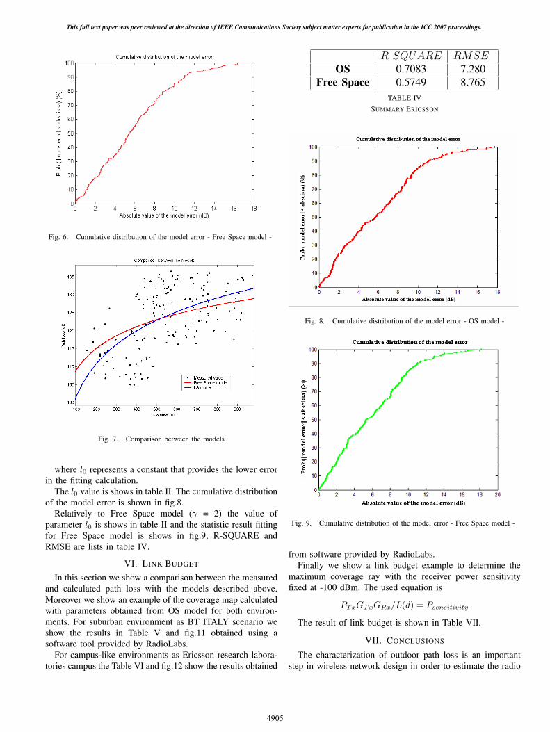
Fig. 6. Cumulative distribution of the model error - Free Space model -

Fig. 7. Comparison between the models

where l0 represents a constant that provides the lower errorin the fitting calculation.

The l0 value is shows in table II. The cumulative distributionof the model error is shown in fig.8.

Relatively to Free Space model (γ = 2) the value ofparameter l0 is shows in table II and the statistic result fittingfor Free Space model is shows in fig.9; R-SQUARE andRMSE are lists in table IV.

VI. LINK BUDGET

In this section we show a comparison between the measuredand calculated path loss with the models described above.Moreover we show an example of the coverage map calculatedwith parameters obtained from OS model for both environ-ments. For suburban environment as BT ITALY scenario weshow the results in Table V and fig.11 obtained using asoftware tool provided by RadioLabs.

For campus-like environments as Ericsson research labora-tories campus the Table VI and fig.12 show the results obtained

R SQUARE RMSEOS 0.7083 7.280

Free Space 0.5749 8.765TABLE IV

SUMMARY ERICSSON

Fig. 8. Cumulative distribution of the model error - OS model -

Fig. 9. Cumulative distribution of the model error - Free Space model -

from software provided by RadioLabs.Finally we show a link budget example to determine the

maximum coverage ray with the receiver power sensitivityfixed at -100 dBm. The used equation is

PTxGTxGRx/L(d) = Psensitivity

The result of link budget is shown in Table VII.

VII. CONCLUSIONS

The characterization of outdoor path loss is an importantstep in wireless network design in order to estimate the radio


4905


Fig. 10. Comparison between the models

Distance(m) Pathloss(dB) OS(dB) FS(dB)1 188.62 108.26 110.10 118.182 294.88 117.54 115.98 122.063 396.39 129.52 119.88 124.634 445.85 121.68 121.42 125.655 495.04 122.92 122.80 126.566 548.22 116.71 124.15 127.447 604.07 135.56 125.42 128.298 695.08 116.49 127.27 129.509 751.24 127.00 128.290 130.1810 863.03 125.450 130.120 131.38

TABLE V

COMPARISON PATH LOSS (BT ITALY)

Fig. 11. Coverage map with OS model (BT ITALY)

coverage and the costs. In this paper we used measureddata to evaluate the parameters of several path loss channelmodels some of them proposed in the current literature. Inparticular, Free space and One Slop models were analyzedand results have been provided for two different categories

Distance(m) Pathloss(dB) OS(dB) FS(dB)1 23.714 69.377 58.290 74.5792 54.337 69.759 71.012 81.7813 80.825 66.569 77.105 85.2304 93.981 90.687 79.418 86.5405 137.11 92.614 85.214 89.8216 222.56 91.265 92.646 94.0287 240.51 97.633 93.837 94.7028 261.15 94.897 95.099 95.4179 346.11 95.828 99.422 97.86310 390.98 93.500 101.29 98.922

TABLE VI

COMPARISON PATH LOSS (ERICSSON)

Fig. 12. Coverage map with OS model (Ericsson Campus)

BTITALY ERICSSONmodel distance(m) distance (m)

OS 996 1570FS 927 1849

TABLE VII

LINK BUDGET: MAXIMUM RAY COVERAGE

of environments: sub-urban and campus-like environment.The comparison between the parameters of the models havebeen shown and the cumulative distribution of the consideredmodels error are also shown. Furthermore in this work isalso shown a link budget example calculated with parametersobtained from OS model for both environments.

REFERENCES

[1] The Business of WiMAX. Deepak Pareek. John Wiley and Soons June2006.

[2] Standard IEEE 802.16d-2004 available on sitehttp://www.ieee802.org/16

[3] Standard IEEE 802.16e-2005 available on sitehttp://www.ieee802.org/16 published on 28 February

[4] V. Erceg, K. V. S. Hari, et al., ”Channel models for fixed wirelessapplications,” tech. rep., IEEE 802.16 Broadband Wireless AccessWorking Group, January 2001

[5] A Survey of Various Propagation Models for Mobile CommunicationTapan K. Sarkar, Zhong Ji, Kyungjung Kim, Abdellatif Medouri, andMagdalena Salazar-Palma IEEE Antennas and Propagation Magazine,Vol.45, No.3,June 2003


4906


Outdoor path loss models for ieee 802.16

Engineering

Transcript of Outdoor path loss models for ieee 802.16