Outcome of systematic research on wind turbine noise in Japan · Outcome of systematic research on...

Inter-noise 2014 of 10

Outcome of systematic research on wind turbine noise in Japan

Hideki TACHIBANA1 1 Professor Emeritus, The University of Tokyo

ABSTRACT

In Japan, serious complaints about wind turbine noise have arisen from nearby residents since the commencement of large-scale construction of wind generation plants in about 2000. Regarding this new type of environmental noise problem, scientific knowledge is insufficient and no standard methods for measuring and assessing the noise have been established in Japan. To improve this situation, a research project entitled “Research on the evaluation of human impact of low frequency noise from wind turbine generators” has been conducted over the three years from fiscal year 2010, funded by a grant from the Ministry of the Environment, Japan. This project consisted of three main subjects: (1) physical research on wind turbine noise by field measurement, (2) a social survey on the response of nearby residents, and (3) auditory experiments on the human response to noises containing low frequency components. In this paper, the outcome of the research project is reviewed and standard methods for measuring and assessing the wind turbine noise are discussed. Keywords: Wind turbine noise, Low frequency sound, Amplitude modulation sound I-INCE Classification of Subjects Number(s): 14.5.4 and 63.2

1. INTRODUCTION In Japan, since the commencement of large-scale construction of wind generation plants in about

2000, serious complaints have arisen from nearby residents regarding wind turbine noise (WTN). Regarding this new type of environmental noise problem, scientific knowledge is insufficient and no standard methods for measuring and assessing the noise have been established in Japan. To improve this situation, a research project entitled “Research on the evaluation of human impact of low frequency noise from wind turbine generators” has been conducted over the three years from fiscal year 2010, funded by a grant from the Ministry of the Environment, Japan (1). This project consisted of three main subjects: 1. physical research on WTN by field measurement, 2. a social survey on the response of nearby residents, and 3. auditory experiments on the human response to noises containing low frequency components. Figure 1 shows the organization of the research groups and the main subjects in the project. In this paper, the outcome of the research project is reviewed by putting emphasis on the field measurements and some technical points for the measurement and assessment of WTN are discussed

1 [email protected]

The Ministry of the Environment, Japan

Research Committee

Secretariat:Chiba Institute of

Technology and INCE/J

WG for Field Measurement

WG for Social Survey

WG for Auditory Experiments

WG for Material Survey

Executive GroupsWest-JapanMiddle-JapanEast-Japan

Acoust. Lab., I.I.S.,Tokyo Univ.

by INCE/JThe Ministry of the Environment, Japan

Research Committee

Secretariat:Chiba Institute of

Technology and INCE/J

WG for Field Measurement

WG for Social Survey

WG for Auditory Experiments

WG for Material Survey

Executive GroupsWest-JapanMiddle-JapanEast-Japan

Acoust. Lab., I.I.S.,Tokyo Univ.

by INCE/J

Figure 1 – Organization of the research groups and the main subjects

of 10 Inter-noise 2014

Page 2 of 10 Inter-noise 2014

2. FIELD MEASUREMENTS OF WTN

2.1 Outline

Regarding WTN problem, no systematic field survey has been conducted in Japan so far except for some case studies on noise complaints about WTN. In this research project, therefore, a systematic investigation was planned and field measurements were conducted for 34 wind farms across Japan. Moreover, to investigate the actual state of residual noise in quiet rural districts, similar measurements were also conducted in 16 control areas with similar local characteristics to the wind farm areas but were not affected by WTN. At the same time as the field measurements, interview-based questionnaires were also conducted both at the wind farm sites and in the control areas to investigate the effect of WTN on nearby residents (2, 3, 4).

From the results of preliminary trials and consideration of the practical conditions at the measurement sites, the following procedures were adopted in the field measurements.

2.2 Measurement Methods and Procedures

In the WTN problem, the effect of low frequency components including infrasound is an important matter of controversy, and therefore prototype wide-frequency-range sound level meters with a measurement frequency range from 1 Hz to 20 kHz and a function for recording the sound pressure signal were used.

To prevent wind-induced noise at a microphone particularly at low frequencies, a prototype wind-screen set shown in Figure 2 was devised. This set is of a double-skin type consisting of a globular wind-screen of 20 cm diameter made of urethane foam and a newly designed dodecahedral second screen covered with a thin cloth (nylon 90% and polyurethane 10%; opening ratio: 60%) with high elasticity. The insertion loss of this wind-screen set is below 1 dB up to 4 kHz as a result of measurement in anechoic room. Its wind-shielding effect was checked by a field measurement in a very quiet plain (1).

The field measurement was performed unattended and continuously for 5 days at each measurement site and the sound pressure was recorded on an SD card installed in the sound level meter.

Although WTN can sometime be audible inside residential buildings potentially disturbing residents’ sleep at night, acoustic measurements inside buildings are very difficult from a physical viewpoint and can invade residents’ privacy. Therefore, it has been decided to perform the measurement facing the nearest wind turbine in the yard of the residence under investigation, and the microphone of the sound level meter covered with the double wind-screen set was placed on the ground so that the center of the microphone was located 20 cm above the ground. The height of the measurement point was decided in order to minimize the effect of wind on the microphone and to avoid various difficulties in keeping the microphone at a high position for a long time (see Figure 2).

In the field measurement around each wind farm, seven measurement positions were uniformly distributed in the residential area within a distance of about 100 m to 1 km from the nearest wind turbine. Moreover, an additional measurement point (reference point) was located near a wind turbine to observe the operation condition of the wind farm.

Figure 2 – An example of field measurement using the double-skin type wind-screen.

16 cm

20 cm

Second wind-screen (DH-160)

Primary wind-screen20 cm, urethane form(RION, WS-03)

½ inchcondenser Microphone

16 cm

20 cm

Second wind-screen (DH-160)

Primary wind-screen20 cm, urethane form(RION, WS-03)

½ inchcondenser Microphone


Inter-noise 2014 Page 3 of 10

2.3 Data Analysis

Data were analyzed by putting priority on nighttime as the reference time interval as shown in Figure 3, since the effect of WTN is generally most severe at night (2) and the effect of the background noise is smallest during this time zone.

At the reference time interval, the recordings for 10 min of every hour during which the wind turbines were judged to be under a rated operation condition were reproduced, and 1/3-octave-band sound pressure levels (SPLs) and A-, C-, and G-weighted time-averaged SPLs were obtained.

When carrying out the analysis, the effect of background noises such as road traffic noise, aircraft noise, and the sounds of various creatures were carefully examined through level recordings and a hearing check for the recorded sounds. If the effect of these background noises was severe, the data were not adopted. In cases where the sounds of insects were dominated in summer and autumn, high-cut filtering was applied to eliminate the frequency components higher than 1.25 kHz in 1/3-octave-band, because the A-weighted SPL is apt to be determined by these sounds.

As the representative values of the 1/3-octave-band and frequency-weighted SPLs for the reference time interval (Lpeq,night), the energy-mean values of the respective SPLs over every 10 min (Lpeq,10min) were calculated.

For the measurements in the control areas, 95 percentile levels of 1/3-octave-band and A-, C-, and G-weighted SPLs over 10 min (Lp95,10min) of every hour at night were obtained, and the representative values (Lp95,night) were calculated as the energy-means of the respective SPLs over every 10 min.

2.4 Measurement Results

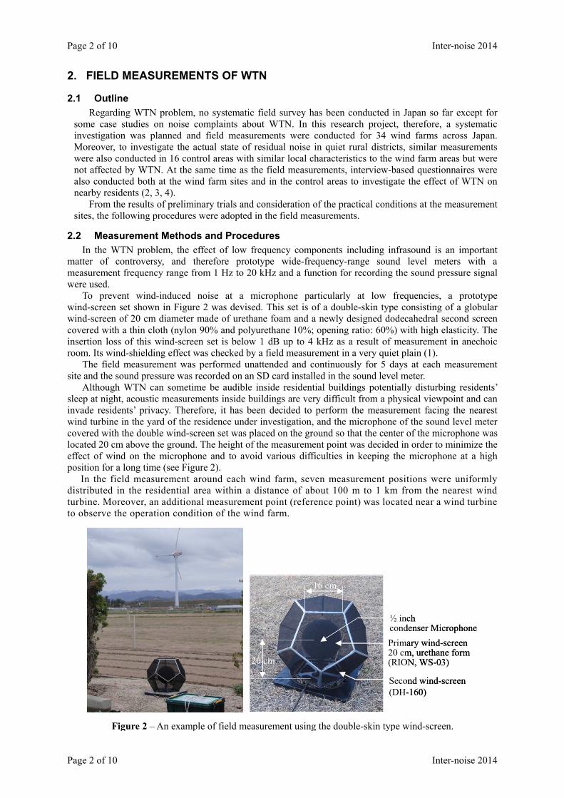
Among the 34 wind farms, the measurement was unsuccessful in the areas around four coastal wind farms being disturbed by sea waves and windbreak. Another measurement was to investigate the emission characteristics of a wind turbine. Excluding these data, time-averaged 1/3-octave-band SPLs measured at 164 points around 29 wind farms are given in Figure 4(a). Brief description of the 29 wind farms is as shown in Table 1. In Figure 4(a), it can be seen that almost all WTNs have similar spectral characteristics, which can be approximated by a slope of - 4 dB/octave in band spectrum. By comparing these results with the criterion curve for the assessment of low frequency noise proposed by Moorhouseet al. (5), it can be seen that the frequency components below 20 Hz for all the WTNs measured in the immission areas were much lower than the curve. The validity of this criterion curve has been confirmed by an auditory experiment on the audibility of low frequency sounds conducted as part of this project (6).

The measurement results of residual noise assessed by 95 percentile level in each 1/3-octave-band at 33 points in 14 control areas are shown in Figure 4(b). Compared to the results for WTNs, the levels were generally much lower and the spectrum characteristics were not uniform.

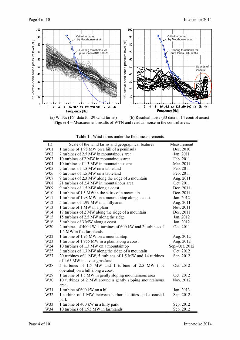
All of the measurement results for LAeq, LCeq, and LGeq are shown in Figure 5 in the form of histograms. In these figures, the data of the residual noise level in terms of LA95, LC95, and LG95 measured at 33 measurement points in the control areas are also shown for comparison. In Figure 5 (a), it can be seen that LAeq for WTN was distributed from 25 dB to 50 dB and the modal class was 41-45 dB. On the other hand, the residual noise level in the control areas was distributed in the ranges from 20 dB to 35 dB. Thus, there was a big difference between the WTN in terms of LAeq and the residual noise in terms of LA95 in the control areas.

Regarding the problem of WTN, the difference between LCeq and LAeq is often discussed. To investigate this point, the relationship between the two indicators was examined using the 164 data. The result is shown in Figure 6, in which it can be seen that LAeq and LCeq had a fairly high correlation.

10 min.

1 hourObservation time interval

Measurement time interval

Reference time interval 8 hours (nighttime)

10 min.

1 hourObservation time interval

Measurement time interval

Reference time interval 8 hours (nighttime)

Figure 3 – Time intervals used for the analysis of WTN.



(a) WTNs (164 data for 29 wind farms) (b) Residual noise (33 data in 14 control areas) Figure 4 – Measurement results of WTN and residual noise in the control areas.

1 2 4 8 16 31.5 63 125 250 500 1k 2k 4k

100

90

80

70

60

50

40

30

20

10

0

- 4 dB/octave

Hearing thresholds for pure tones (ISO 389-7）

Criterion curveby Moorhouse et al.

1/3-

octa

ve-b

and

soun

d pr

essu

re le

vel [

dB]

Frequency [Hz]1 2 4 8 16 31.5 63 125 250 500 1k 2k 4k1 2 4 8 16 31.5 63 125 250 500 1k 2k 4k

100

90

80

70

60

50

40

30

20

10

0

100

90

80

70

60

50

40

30

20

10

0

- 4 dB/octave

- 4 dB/octave



1/3-

octa

ve-b

and

soun

d pr

essu

re le

vel [

dB]

Frequency [Hz]

1 2 4 8 16 31.5 63 125 250 500 1k 2k 4k

Frequency [Hz]

100

90

80

70

60

50

40

30

20

10

0

1/3-

octa

ve-b

and

soun

d pr

essu

re le

vel [

dB]

Sounds of insects- 4 dB/octave



1 2 4 8 16 31.5 63 125 250 500 1k 2k 4k1 2 4 8 16 31.5 63 125 250 500 1k 2k 4k

Frequency [Hz]

100

90

80

70

60

50

40

30

20

10

0

100

90

80

70

60

50

40

30

20

10

0

1/3-

octa

ve-b

and

soun

d pr

essu

re le

vel [

dB]





- 4 dB/octave



1 2 4 8 16 31.5 63 125 250 500 1k 2k 4k

100

90

80

70

60

50

40

30

20

10

0

- 4 dB/octave



1/3-

octa

ve-b

and

soun

d pr

essu

re le

vel [

dB]

Frequency [Hz]1 2 4 8 16 31.5 63 125 250 500 1k 2k 4k1 2 4 8 16 31.5 63 125 250 500 1k 2k 4k

100

90

80

70

60

50

40

30

20

10

0

100

90

80

70

60

50

40

30

20

10

0

- 4 dB/octave

- 4 dB/octave



1/3-

octa

ve-b

and

soun

d pr

essu

re le

vel [

dB]

Frequency [Hz]

1 2 4 8 16 31.5 63 125 250 500 1k 2k 4k

Frequency [Hz]

100

90

80

70

60

50

40

30

20

10

0

1/3-

octa

ve-b

and

soun

d pr

essu

re le

vel [

dB]




1 2 4 8 16 31.5 63 125 250 500 1k 2k 4k1 2 4 8 16 31.5 63 125 250 500 1k 2k 4k

Frequency [Hz]

100

90

80

70

60

50

40

30

20

10

0

100

90

80

70

60

50

40

30

20

10

0

1/3-

octa

ve-b

and

soun

d pr

essu

re le

vel [

dB]





- 4 dB/octave



Table 1 - Wind farms under the field measurements

ID Scale of the wind farms and geographical features Measurement W01 1 turbine of 1.98 MW on a hill of a peninsula Dec. 2010 W02 7 turbines of 2.5 MW in mountainous area Jan. 2011 W03 10 turbines of 2 MW in mountainous area Feb. 2011 W04 10 turbines of 1.3 MW in mountainous area Mar. 2011 W05 9 turbines of 1.5 MW on a tableland Feb. 2011 W06 6 turbines of 1.5 MW on a tableland Feb. 2011 W07 9 turbines of 2.3 MW along the ridge of a mountain Aug. 2011 W08 21 turbines of 2.4 MW in mountainous area Oct. 2011 W09 9 turbines of 1.5 MW along a coast Dec. 2011 W10 1 turbine of 1.5 MW in the skirts of a mountain Dec. 2011 W11 1 turbine of 1.98 MW on a mountaintop along a coast Jan. 2012 W12 5 turbines of 1.99 MW in a hilly area Aug. 2011 W13 1 turbine of 1 MW in a plain Nov. 2011 W14 17 turbines of 2 MW along the ridge of a mountain Dec. 2011 W15 15 turbines of 2.5 MW along the ridge Jan. 2012 W16 5 turbines of 3 MW along a coast Jan. 2012 W20 2 turbines of 400 kW, 4 turbines of 600 kW and 2 turbines of

1.5 MW in flat farmlands Oct. 2011

W22 1 turbine of 1.95 MW on a mountaintop Aug. 2012 W23 1 turbine of 1.955 MW in a plain along a coast Aug. 2012 W24 10 turbines of 1.3 MW on a mountaintop Sep.-Oct. 2012 W25 8 turbines of 1.3 MW along the ridge of a mountain Oct. 2012 W27 20 turbines of 1 MW, 5 turbines of 1.5 MW and 14 turbines

of 1.65 MW in a vast grassland Sep. 2012

W28 5 turbines of 1.5 MW and 1 turbine of 2.5 MW (not operated) on a hill along a coast

Oct. 2012

W29 1 turbine of 1.5 MW in gently sloping mountainous area Oct. 2012 W30 10 turbines of 2 MW around a gently sloping mountainous

area Nov. 2012

W31 1 turbine of 600 kW on a hill Jan. 2013 W32 1 turbine of 1 MW between harbor facilities and a coastal

park Sep. 2012

W33 1 turbine of 400 kW in a hilly park Sep. 2012 W34 10 turbines of 1.95 MW in farmlands Sep. 2012



In Figure 5(c), it is clear that the G-weighted sound pressure levels measured in the areas around wind farms were higher than those measured in the control areas. Even in the areas around wind farms, however, the levels were much lower than the infrasound threshold level described in ISO 7196.

Figure 5 – WTNs and residual noise in the control areas.

Figure 6 – Correlation between LAeq and LCeq of WTN

20

30

40

50

60

70

20 30 40 50 60 70LAeq [dB]

y = 0.83x + 21.90R= 0.88

L Ce

q[d

B]

20

30

40

50

60

70

20 30 40 50 60 70LAeq [dB]

y = 0.83x + 21.90R= 0.88

L Ce

q[d

B]

11-1

5

16-2

0

21-2

5

26-3

0

31-3

5

36-4

0

41-4

5

46-5

0

51-5

5

80

70

60

50

40

30

20

10

0

Fre

quen

cy

LAeq or LA,95 [dB]

(a) LAWind farm areas (164 data), in LAeq

Control areas (33 data), in LA,95

31-3

5

36-4

0

41-4

5

46-5

0

51-5

5

56-6

0

61-6

5

66-7

0

71-7

5

80

70

60

50

40

30

20

10

0

Fre

quen

cy

LGeq or LG,95 [dB]

(c) LGWind farm areas (164 data), in LAeq


26-3

0

31-3

5

36-4

0

41-4

5

46-5

0

51-5

5

56-6

0

61-6

5

66-7

0

80

70

60

50

40

30

20

10

0

Fre

quen

cy

LCeq or LC,95 [dB]

(b) LCWind farm areas (164 data), in LAeq


11-1

5

16-2

0

21-2

5

26-3

0

31-3

5

36-4

0

41-4

5

46-5

0

51-5

5

80

70

60

50

40

30

20

10

0

Fre

quen

cy

LAeq or LA,95 [dB]



11-1

5

16-2

0

21-2

5

26-3

0

31-3

5

36-4

0

41-4

5

46-5

0

51-5

5

80

70

60

50

40

30

20

10

0

Fre

quen

cy

LAeq or LA,95 [dB]



Wind farm areas (164 data), in LAeq


31-3

5

36-4

0

41-4

5

46-5

0

51-5

5

56-6

0

61-6

5

66-7

0

71-7

5

80

70

60

50

40

30

20

10

0

Fre

quen

cy

LGeq or LG,95 [dB]



31-3

5

36-4

0

41-4

5

46-5

0

51-5

5

56-6

0

61-6

5

66-7

0

71-7

5

80

70

60

50

40

30

20

10

0

Fre

quen

cy

LGeq or LG,95 [dB]





26-3

0

31-3

5

36-4

0

41-4

5

46-5

0

51-5

5

56-6

0

61-6

5

66-7

0

80

70

60

50

40

30

20

10

0

Fre

quen

cy

LCeq or LC,95 [dB]



26-3

0

31-3

5

36-4

0

41-4

5

46-5

0

51-5

5

56-6

0

61-6

5

66-7

0

80

70

60

50

40

30

20

10

0

Fre

quen

cy

LCeq or LC,95 [dB]







To see the SPL distribution in distance, LAeq,night was examined as a function of the distance from the wind turbine for all of the measurement data shown in Figure 4(a). The results are shown in Figure 7(a) for single wind turbines (51 points at 10 sites) and in Figure 7(b) for wind farms with more than one wind turbine (113 points at 19 sites). These results show that the sound level tends to gradually decrease with increasing distance, but the plots are scattered. WTN propagation is generally very complicated owing not only to meteorological conditions but also to topographical condition, vegetation condition, etc. Especially in Japan, wind power plants are often constructed in hilly areas and the sound propagation is very complicated.

3. AMPLITUDE MODULATION When the blades of a wind turbine rotate, they generate a periodic fluctuating sound, the so-called

“amplitude modulation (AM) sound” or “swish sound”, and such sounds much increase psychological annoyance (7, 8). AM sound is related to the directivity of the aerodynamic trailing edge noise and Doppler amplification, and its main frequency components audible in immission areas are in the mid-frequency range (about 400 to 1000 Hz) (7).

To objectively quantify the level of AM, several methods have been proposed (9-12), in which the frequency and magnitude of the envelope of amplitude modulation are detected by applying sophisticated signal processing techniques. As another method, the authors adopted a very simple and practical method in this study as described below.

Figure 8(a) shows an example of the A-weighted sound pressure levels of WTN recorded with FAST and SLOW time-weightings for 3 min. The data were measured at a point 1,152 m from a 1.95 MW wind turbine. In this case, it is clearly seen that the mean sound pressure level varied with time. Therefore, it is necessary to find a suitable method for quantitatively assessing the strength of AM over a long time. As a simple idea to achieve this, the difference between the A-weighted sound pressure level with FAST time-weighting (LA,F(t)) and that with SLOW time-weighting (LA,S(t)) is calculated as

)()()( SA,FA,A tLtLtL (1).

Then, the width of the 90% range of the level difference is obtained as a measure indicating the AM depth.

95A5AAM LLD (2)

where, DAM is the AM depth in dB, and LA5 and LA95 are the 5% and 95% levels of LA(t), respectively. Figure 8(b) shows a magnification of the recording in Figure 8(a) over 40 s, and the level difference

between the FAST and SLOW time-weightings is shown in Figure 8(c). Figures 9(a) and 9(b) show the auto-correlation coefficient and the auto-power spectrum calculated for the level difference LA(t) for 3 min shown in Figure 8(c). In these results, it can be clearly seen that the level difference had a dominant spectrum at 1.03 Hz, which corresponds to the blade passing frequency of the turbine under measurement. Figure 8(d) shows the procedure to determine DAM,. In this case, DAM is 2.8 dB.

The above procedure was applied to the sound pressure recordings made at 81 points at 18 wind farm sites. As a result, it was found that amplitude modulation depth (DAM) ranged from 1 dB to 5 dB and that the modal group was 2.0 to 2.4 dB as shown in Figure 10. It is known that the sensation of fluctuation begins at an AM depth of approximately 2 dB (7). This was confirmed in a recent auditory experiment performed as part of this research project (13). According to these findings, fluctuation due to AM can be detected at about three-quarters of the measurement points examined in this study.

Figure 7 – Distribution in distance of WTN

20

30

40

50

60

0 250 500 750 1000 1250 150020

30

40

50

60

0 250 500 750 1000 1250 1500

(b) Wind farms

Distance from the nearest wind turbine [m]L A

eq,n

ight

[dB

]Distance from the wind turbine [m]

20

30

40

50

60

0 250 500 750 1000 1250 150020

30

40

50

60

0 250 500 750 1000 1250 1500

L Aeq

,nig

ht[d

B]

(a) Single WT

20

30

40

50

60

0 250 500 750 1000 1250 150020

30

40

50

60

0 250 500 750 1000 1250 1500

(b) Wind farms

Distance from the nearest wind turbine [m]L A

eq,n

ight

[dB

]Distance from the wind turbine [m]

20

30

40

50

60

0 250 500 750 1000 1250 150020

30

40

50

60

0 250 500 750 1000 1250 1500

L Aeq

,nig

ht[d

B]

(a) Single WT



Figure 8 – An example of objective quantification of the level of Amplitude Modulation.(a) A-weighted SPL recorded with FAST and SLOW time-weightings for 3 min, (b) magnification of recording shown in (a) over 40 s, (c) level difference between FAST and SLOW, and (d) statistical determination of AM depth (DAM) from the level difference shown in (c).

FAST SLOW40

35

30

25

20

L A(t

) [d

B] (b)

130 140 150 160 170Time [s]

0 30 60 90 120 150 180Time [s]

(a) FAST SLOW40

35

30

25

20

L A(t

) [d

B]

130 140 150 160 170Time [s]

ΔL A

(t)

[dB

] (c)

FAST SLOW40

35

30

25

20

L A(t

) [d

B] (b)

130 140 150 160 170Time [s]

FAST SLOWFAST SLOW40

35

30

25

20

L A(t

) [d

B] (b)

130 140 150 160 170Time [s]

0 30 60 90 120 150 180Time [s]

(a) FAST SLOW40

35

30

25

20

L A(t

) [d

B]

0 30 60 90 120 150 180Time [s]

(a) FAST SLOWFAST SLOW40

35

30

25

20

L A(t

) [d

B]

130 140 150 160 170Time [s]

ΔL A

(t)

[dB

] (c)

130 140 150 160 170Time [s]

ΔL A

(t)

[dB

] (c)

Cumulative distribution

Probability density

DAM

ΔLA,5ΔLA,95

100

80

60

40

20

0

Cum

ulat

ive

dist

ribut

ion

[%]

-5 -4 -3 - 2 -1 0 1 2 3 4 5

Level difference : ΔLA [dB]

Pro

bab

ility

den

sity

[%

]

10

8

6

4

2

0

90 %

ran

ge

(d)


Probability density

DAM

ΔLA,5ΔLA,95

100

80

60

40

20

0

Cum

ulat

ive

dist

ribut

ion

[%]

-5 -4 -3 - 2 -1 0 1 2 3 4 5


Pro

bab

ility

den

sity

[%

]

10

8

6

4

2

0

90 %

ran

ge


Probability density

DAM

ΔLA,5ΔLA,95

100

80

60

40

20

0

Cum

ulat

ive

dist

ribut

ion

[%]

-5 -4 -3 - 2 -1 0 1 2 3 4 5


Pro

bab

ility

den

sity

[%

]

10

8

6

4

2

0

90 %

ran

ge

(d)

0.15

0.10

0.05

0.00

Frequency Hz]0 0.5 1 1.5 2 2.5

Aut

o-po

we

r sp

ectr

um

0.15

0.10

0.05

0.00

Frequency Hz]0 0.5 1 1.5 2 2.5

Aut

o-po

we

r sp

ectr

um

0.0 1.0 2.0 3.0 4.0 5.0

Time delay τ [s]

1.0

0.5

0.0

-0.5

-1.0

Aut

oco

rrel

atio

n co

effi

cie

nt

0.0 1.0 2.0 3.0 4.0 5.0

Time delay τ [s]

1.0

0.5

0.0

-0.5

-1.0

Aut

oco

rrel

atio

n co

effi

cie

nt

(a) Autocorrelation coefficient (b) Auto-power spectrum

0.15

0.10

0.05

0.00

Frequency Hz]0 0.5 1 1.5 2 2.5

Aut

o-po

we

r sp

ectr

um

0.15

0.10

0.05

0.00

Frequency Hz]0 0.5 1 1.5 2 2.5

Aut

o-po

we

r sp

ectr

um

0.0 1.0 2.0 3.0 4.0 5.0

Time delay τ [s]

1.0

0.5

0.0

-0.5

-1.0

Aut

oco

rrel

atio

n co

effi

cie

nt

0.0 1.0 2.0 3.0 4.0 5.0

Time delay τ [s]

1.0

0.5

0.0

-0.5

-1.0

Aut

oco

rrel

atio

n co

effi

cie

nt

(a) Autocorrelation coefficient (b) Auto-power spectrum

1.0 –

1.4

2.5

–2.9

2.0

–2.4

1.5

–1.9

3.0

–3.4

3.5

–3.9

4.0

–4.4

4.5

–4.

95.

0 –

–0.9

30

25

20

15

10

5

0

Amplitude modulation depth : DAM [dB]

Fre

quen

cy

AM sound is audible

1.0 –

1.4

2.5

–2.9

2.0

–2.4

1.5

–1.9

3.0

–3.4

3.5

–3.9

4.0

–4.4

4.5

–4.

95.

0 –

–0.9

30

25

20

15

10

5

0


Fre

quen

cy

1.0 –

1.4

2.5

–2.9

2.0

–2.4

1.5

–1.9

3.0

–3.4

3.5

–3.9

4.0

–4.4

4.5

–4.

95.

0 –

–0.9

30

25

20

15

10

5

0


Fre

quen

cy

AM sound is audible

Figure 10 – Distribution of AM depth, DAM, in the data measured at 81 points in the areas around 18wind farms.

Figure 9 – Autocorrelation function and auto-power spectrum of the level difference LA(t).



4. INDICATOR FOR WTN ASSESSMENT Noise limits or guidelines for WTN are legislated in many countries, states, and provinces, and almost

all legislations are specified in terms of the A-weighted SPL, in common with general environmental noises. Regarding the A-weighted SPL, however, many critical arguments have been made (14-16). In particular, for WTN with relatively dominant low-frequency components, the applicability of the A-weighted SPL needs to be reexamined experimentally. For this aim, we conducted a basic loudness test using various environmental noises including WTN that were recorded so as to include low-frequency components down to infrasound and were reproduced in an experimental facility capable of reproducing low frequency sounds down to 4 Hz (17). The experimental results were evaluated using the A- and C-weighted SPLs, Zwicker loudness level, and Moore-Glasberg loudness level. As a result, it has been found that the A-weighted SPL is a simple and appropriate indicator for the loudness assessment of general environmental noise. In the results of other auditory experiments we conducted in this research project, the applicability of the A-weight SPL to the assessment of perceived loudness of sounds with dominant components at low frequencies has been found (6). These facts might suggest that the A-weight SPL can be used in the assessment of WTN as a primary indicator.

5. EFFECTS OF BACKGROUND NOISE In the field measurements in this study, the time-averaged A-weighted SPL was obtained as mentioned

above, but it is a hard job and needs close attention to eliminate the background noise because the level of WTN in immission areas is relatively low. A practical way to avoid such a problem is to obtain the 90% or 95% value of the A-weighted SPL for the measurement time interval. Figure 10 shows the relationship between (a) LAeq,3min and LA90,3min and (b) LAeq,3min and LA95,3min of WTNs measured at 81 points around 18 wind farms. Here, the effect of the background noise was eliminated when measuring LAeq. In both cases, a considerably high correlation is seen between the respective indicators. This means that LAeq can be approximated by adding 2.2 dB to LA90 or 2.6 dB to LA95. Strictly speaking, the difference between LAeq and LA90 or LA95 depends on the level of the amplitude modulation, but its effect can practically be neglected when considering general WTNs in immission areas around wind farms.

6. CONCLUSIONS As a result of the systematic research on WTN in Japan conducted to obtain fundamental material to

produce guidelines of noise impact assessment of wind power plants, the following findings have been obtained.

(a) LAeq,3min vs. LA90,3min (b) LAeq,3min vs. LA95,3min

Figure 10 – Relationship between LAeq,3min (the effect of the background noise was eliminated) and LA90,3min or LA95,3min of WTNs measured at 81 points at 18 wind farm sites.

y = 0.997 x + 2.580

R 2 =.984

20

30

40

50

60

70

20 30 40 50 60 70

LA95,3min [dB]

L Aeq

,3m

in [d

B]

y = 0.996 x + 2.201

R 2 = 0.989

20

30

40

50

60

70

20 30 40 50 60 70LA90,3min [dB]

L Aeq

,3m

in [d

B]

y = 0.997 x + 2.580

R 2 =.984

20

30

40

50

60

70

20 30 40 50 60 70

LA95,3min [dB]

L Aeq

,3m

in [d

B]

y = 0.996 x + 2.201

R 2 = 0.989

20

30

40

50

60

70

20 30 40 50 60 70LA90,3min [dB]

L Aeq

,3m

in [d

B]



(1) Acoustical characteristics of WTN: From the measurement results obtained at 164 points in the residential areas around 29 wind farms, it was found that WTN generally has a spectrum characteristic of about - 4 dB/octave in band spectrum and the components in the infrasound frequency region were much below the hearing thresholds. This fact was examined through a laboratory experiment conducted as part of this research project (6). These indicate that WTN is not a problem in the infrasound frequency region. However, most of the frequency components in audible frequency range are above the hearing thresholds. This means that WTN should be discussed as an “audible” environmental noise.

(2) Noise effects: All the measurement results of WTN in the immission areas obtained in this study were between 25 dB to 50 dB at most in terms of LAeq. Although these levels are not so high compared with other community noises, they are audible, especially at night, and might cause serious annoyance and sleep disturbance in residential areas which are generally very quiet rural districts. Legislative and administrative measures (noise limits or guidelines) should be prepared by considering these points.

(3) Noise indicator: WTN can be assessed by the A-weighted SPL as a primary indicator, similarly to general environmental noises. Since WTN is relatively low level in general, it is rather difficult to accurately measure LAeq being influenced by various background noises. In this respect, it is preferable to measure the percentile level like LA90 or LA95 from which LAeq can be approximated statistically.

(4) Amplitude modulation: Amplitude modulation generated by the rotation of the blades of wind turbine is inevitable in WTN, and is apt to increase residents’ annoyance. Therefore, the effect of AM sound should be considered when preparing noise limit or guideline for WTN (18). To objectively assess the extent of amplitude modulation, a simple statistical method was proposed in this research project.

(5) Tonal components: In the measurement results of this study, tonal components were observed in some cases, especially in the areas near some types of wind turbines. Tonality is also a serious factor to increase annoyance of WTN (19, 20) and the effect should be considered as an additional penalty when any tonal components are included in WTN (18). The method for objectively assessing the tonality is specified in IEC 61400-11: 2012 and is also being discussed at ISO/TC43. The effectiveness of these assessment methods are being investigated also in Japan.

(6) Measurement points: For some physical and practical reasons as mentioned in 2.2, the measurement points should be located outside of buildings in principle. In the measurement, the microphone should be covered with wind-screen with a high wind-shielding effect and be placed close to the ground in order to prevent the wind-induced noise as far as possible.

(7) Residual noise: In the WTN problem, the audibility of the noise when the environment is quiet is serious. Therefore, the environmental condition without WTN should be assessed by the residual noise which is an ambient noise excluding every specific noise such as road traffic noise, aircraft noise, and the sounds of various creatures. To that end, 90 or 95 percentile level should be measured and used in the assessment of the environmental condition.

ACKNOWLEDGEMENTS This research project was financed by a grant from the Ministry of the Environment, Japan. The author

gratefully acknowledges the members of the Research Committee of the project for their wholehearted cooperation. The author also thanks Mr. Tatsuya Ohta at NEWS Environmental Design Inc. and Dr. Tomohiro Kobayashi at Kobaysi Institute of Physical Research for their technical assistance in this study.

REFERENCES 1. H. Tachibana, H. Yano, A. Fukushima and S. Sueoka, “Nationwide field measurements of wind turbine

noise in Japan”, Noise Control Eng. J., 62(2), 90-101 (2014). 2. S. Kuwano, T. Yano, T. Kageyama, S. Sueoka and H. Tachibana, “Social survey on community

response to wind turbine noise in Japan”, Inter-Noise 2013 (2013). 3. T. Yano, S. Kuwano, T. Kageyama, S. Sueoka and H. Tachibana, “Dose-response relationships for wind

turbine noise in Japan”, Inter-Noise 2013 (2013). 4. T. Kageyama, T. Yano, S. Kuwano, S. Sueoka and H. Tachibana, “Exposure-response relationship of

wind turbine noise with subjective symptoms on sleep and health: a nationwide socio-acoustic survey in Japan”, ICBEN 2014 (2014).



5. A. T. Moorhouse, D. C. Waddington and M. D. Adams, “A procedure for the assessment of low frequency noise complaints”, J. Acoust. Soc. Am., 126(3), 1131-1141 (2009).

6. S. Yokoyama, S. Sakamoto and H. Tachibana, “Perception of low frequency components contained in wind turbine noise”, Wind Turbine Noise 2013 (2013).

7. D. Bowdler and G. Leventhall, Wind Turbine Noise, Chapter 5, Multi-Science Publishing Co. Ltd. (2011).

8. J. Bass, D. Bowdler, M. McCaffery and G. Grimes, “Fundamental research in amplitude modulation – a project by RenewableUK”, 15th International Meeting on Low Frequency Noise and Vibration and its Control (2012).

9. S. Lee, K. Kim, W. Choi and S. Lee, “Annoyance caused by amplitude modulation of wind turbine noise”, Noise Control Eng. J., 59(1) (2011).

10. J. N. McCabe, “Detection and quantification of amplitude modulation in wind turbine noise”, Wind Turbine Noise 2011 (2011).

11. D. McLaughlin, “Measurement of amplitude modulation frequency spectrum”, Wind Turbine Noise 2011 (2011).

12. G. Lundmark, “Measurement of swish noise, a new method”, Wind Turbine Noise 2011 (2011). 13. S. Yokoyama, S. Sakamoto, and H. Tachibana, “Study on the amplitude modulation of wind turbine

noise: part 2 – Auditory experiments”, Inter-Noise 2013 (2013). 14. R. Hellman and E. Zwicker, “Why can a decrease in dB(A) produce an increase in loudness?”, J.

Acoust. Soc. Am., 82(5), 1700-1705 (1987). 15. S. Kuwano and S. Namba, “Advantages and Disadvantages of A-weighted SPL in Relation to

Subjective Impression of Environmental Noises”, Noise Control Eng. J., 33(3), 107-115 (1989). 16. R. L. St. Pierre, Jr. and D. J. Maguire, “The impact of A-weighting SPL measurements during the

evaluation of noise exposure,” NOISE-CON 2004 (2004). 17. S. Sakamoto, S. Yokoyama, S. Tsujimura, and H. Tachibana, “Loudness evaluation of general

environmental noise containing low frequency components”, Inter-Noise 2013 (2013). 18. Standards New Zealand NZS 6808 Acoustics – Wind farm noise (2010). 19. J. Cooper, T. Evans and D. Petersen, “Tonality assessment at a residence near a wind farm”, Wind

Turbine Noise 2013 (2013). 20. L. S. Søndergaard and T. H. Pedersen, “Tonality in wind turbine noise. IEC 61400-11 ver. 2.1 and 3.0

and the Danish/Joint Nordic method compared with listening tests”, Wind Turbine Noise 2013 (2013).

Outcome of systematic research on wind turbine noise in Japan · Outcome of systematic research on...

Documents

Transcript of Outcome of systematic research on wind turbine noise in Japan · Outcome of systematic research on...