OUT-OF-SCHOOL SUSPENSIONS BY HOME NEIGHBORHOOD: by …

OUT-OF-SCHOOL SUSPENSIONS BY HOME NEIGHBORHOOD:

A SPATIAL ANALYSIS OF STUDENT SUSPENSIONS

IN THE SAN BERNARDINO CITY UNIFIED SCHOOL DISTRICT

by

Stephen O. Gervais

A Thesis Presented to the

FACULTY OF THE USC GRADUATE SCHOOL

UNIVERSITY OF SOUTHERN CALIFORNIA

In Partial Fulfillment of the

Requirements for the Degree

MASTER OF SCIENCE

(GEOGRAPHIC INFORMATION SCIENCE AND TECHNOLOGY)

December 2012

Copyright 2012 Stephen O. Gervais

ii

Acknowledgements

I wish to acknowledge the extended and long-term support of the instructors and staff of

the USC Spatial Sciences Institute, especially Dr. John P. Wilson, my thesis committee

chairman and Director of the USC Spatial Sciences Institute.

I also wish to acknowledge the encouragement and support of the staff of the

Research Office of the San Bernardino City Unified School District (SBCUSD). In

particular, I wish to thank my past and present supervisors, Dr. Paul Shirk, Mrs. Karla

Maez, and Mrs. Barbara Richardson, and my co-worker, Mrs. Cindi Blair. They have

been very supportive of my studies in GIScience and instrumental in granting me access

to the SBCUSD datasets used for this thesis project.

Most importantly, I would like to thank my family members, especially my wife,

Nancy, and my sons, Kenneth and Jonathan, for their endless support, patience and

extreme understanding while I have pursued this degree.

iii

Table of Contents

Acknowledgements ii

List of Tables v

List of Figures vi

Abstract viii

Chapter 1 Introduction 1

1.1 The Problem of Out-of-School Suspensions 1

1.2 Description of the Study Area 4

1.3 Organization of the Thesis 16

Chapter 2 Literature Review 17

2.1 Suspensions: Definition and Policies 17

2.2 Who Gets Suspended? 19

2.3 Neighborhoods and Suspensions 21

2.4 Social Disorder Theory 24

Chapter 3 Methods and Data Sources 26

3.1 Preparation of the SBCUSD Map 27

3.2 Preparation of the SBCUSD Student Dataset 28

3.3 Geocoding the Dataset and Defining an Appropriate Study Area 31

3.4 Visualizing SBCUSD Enrollment and Suspension Incident Rates 32

3.5 Spatial Analysis of the SBCUSD Suspension Incidents 34

3.5.1 Measuring Spatial Autocorrelation using Moran’s Global I 34

3.5.2 Getis-Ord Gi*(d) Hot-Spot Analysis 36

3.5.3 Hot-Spot Summary Using Spatial Intersection 38

3.5.4 Neighborhood Hot-Spot Grouping Patterns 39

3.6 Suspension Modeling Using Regression 40

3.6.1 Exploratory Regression Analysis 40

3.6.2 Ordinary Least Squares (OLS) Regression 42

3.6.3 Geographically Weighted Regression 42

iv

Chapter 4 Results 44

4.1 Patterns in Student Enrollment 44

4.2 Analysis of Student Suspensions 48

4.2.1 Spatial Autocorrelation of Suspension Incidents 49

4.2.2 Hot Spot Analysis of Suspensions – Detailed Example and

Summary 49

4.2.3 Neighborhood Hot Spot Grouping Patterns 53

4.3 Modeling Suspension Incident Rates Using Regression Analysis 57

4.3.1 Exploratory Regression Analysis 58

4.3.2 Ordinary Least-Square (OLS) Regression 59

4.3.3 Geographically Weighted Regression 61

Chapter 5 Discussion and Conclusions 65

5.1 Patterns in Student Enrollment 65

5.2 Analysis of Student Suspensions 67

5.3 Modeling Suspension Incident Rates Using Regression Analysis 68

5.4 Final Comments 69

References 70

Appendix 1 SBCUSD Notice of Suspension 74

Appendix 2 SBCUSD Suspension Incident Rank Reporting Plan 75

Appendix 3 OLS Summary of Results 76

Appendix 4 GWR Model by Census Block Group 77

v

List of Tables

Table 1: US suspension rates by gender and race/ethnicity, 2000 - 2006 2

Table 2: A comparison of 2010 national, state and local poverty rates 8

Table 3: SBCUSD students receiving free or reduced price meals 8

Table 4: SBCUSD English Learner enrollment 9

Table 5: Percent of tested students scoring proficient in ELA 10

Table 6: Percent of tested students scoring proficient in MATH 10

Table 7: Percent of annual student dropouts, grades 9-12 11

Table 8: SBCUSD 2009-10 suspension incident types by frequency 13

Table 9: SBCUSD 2009-10 suspension incident rates by level and ethnicity 15

Table 10: SBCUSD 2009-10 enrollment record layout 29

Table 11: SBCUSD 2009-10 suspension incident summary record layout 30

Table 12: SBCUSD 2009-10 enrollment by elementary school neighborhood 46

Table 13: Distance bands with most significant clustering of suspension incidents

by subgroup 49

Table 14: Percent of neighborhood hotspot incident clustering by elementary school

neighborhood and suspension incident category 52

Table 15: Elementary school neighborhoods – group pattern 1 53





Table 20: Exploratory regression summary of variable significance 58

vi

List of Figures

Figure 1: San Bernardino City USD, schools and boundaries 5

Figure 2: SBCUSD student enrollment (October census) 6

Figure 3: SBCUSD enrollment by ethnicity (October census) 6

Figure 4: SBCUSD student suspension rate history 14

Figure 5: SBCUSD incident rates by CBEDS grade 15

Figure 6: Lincoln Elementary School neighborhood boundaries 28

Figure 7: SBCUSD suspension study area 32

Figure 8: Moran's Global I for suspensions incidents classified as defiance -

EC 48900(k) 36

Figure 9: Hot-spot summary model using spatial intersection 38

Figure 10: Scatterplot matrix: Suspension model factors 41

Figure 11: SBCUSD 2009-10 enrollment by census block groups 44

Figure 12: Enrollment by subgroup - 1 standard deviation distribution from center 47

Figure 13: SBCUSD 2009-10 incident rate by census block groups 48

Figure 14: Hotspot analysis by census block groups using Getis-Ord Gi* statistic 50

Figure 15: 2009-10 School Year suspension grouping patterns 54

Figure 16: OLS regression model standardized residuals 60

Figure 17: GWR model standardized residuals 61

Figure 18: GWR model adjusted local R2 62

Figure 19: GWR Coefficient #1 - CBEDS enrollment total days suspended 2008-09 62

Figure 20: GWR Coefficient #2 - CBEDS enrollment identified as LowSES 63

vii

Figure 21: 2009-10 observed suspension incidents 64

Figure 22: 2009-10 predicted suspension incidents, GWR Model 64

viii

Abstract

Student out-of-school suspensions have been an ongoing problem in US schools for many

years. Current methods of analysis have not yielded new insights into this problem. The

purpose of this thesis is to consider student suspension incidents from a spatial

perspective. Using student level data provided by SBCUSD, a large urban school district

in southern California, suspension incidents were geocoded and mapped to student home

neighborhoods within the district for the purpose of identifying whether or not

suspensions incidents are clustered and, if so, to determine by neighborhood where the

clusters are located. Spatial analysis indicated that suspension incident clustering does

exist. Hotspot analysis showed variations in the suspension incident clustering pattern

when disaggregating results by significant student subgroups and incident types.

Neighborhoods were classified by these patterns and the results visualized in a choropleth

map. As a final step in the analysis, a geographically weighted regression model

predicting districtwide suspension incidents by census block group was developed. The

model, based on the total number of days previously suspended and the number of

students identified as having a low socioeconomic status, had an adjusted R2 greater than

0.90. Additional research needs to be conducted to verify that the patterns noted within

this thesis hold steady. If so, discipline issues within SBCUSD may in part be

influenced by local neighborhood factors. This becomes an opportunity for the school

district to act at a local level and identify strategies to reduce suspensions and improve

student outcomes.

1

Chapter 1

Introduction

1.1 The Problem of Out-of-School Suspensions

Student discipline has been an ongoing problem in US schools for many years. In the past

60 years since formal records have been kept, student discipline has been a top problem

continually reported by educators (Brodbelt 1978; Wu et al. 1982; Bowditch 1993;

Mendez and Knoff 2003; Krezmien et al. 2006).

At first glance, the issue seems simple. Schools and school districts must establish

rules for behavior to maintain an orderly education environment and to ensure the safety

of all students. When a student is caught breaking the rules, the student is punished.

Simple infractions may result in a phone call to a student’s parents or guardians while

more extreme violations of the rules can result in out-of-school suspension and, in some

cases, expulsion. The focus of this thesis is on those extreme violations by students which

result in an out-of-school suspension of one or more days of school.

According to the US Department of Education (Planty et al. 2009) during the

period 2000 - 2006, male students were suspended at a rate more than twice that of

females. African American students were suspended at a rate more than twice Hispanic

students and more than three times that of White students. Table 1 details suspension

rates over this time period by gender and race/ethnicity.

2

Table 1: US suspension rates by gender and race/ethnicity, 2000 - 2006

2000 2002 2004 2006

Gender

Male 9.2% 9.0% 9.2% 9.1%

Female 3.9% 4.0% 4.3% 4.5%

Race/Ethnicity

African Am 13.3% 13.9% 15.0% 15.0%

Hispanic 6.1% 6.0% 6.5% 6.8%

White 5.1% 4.9% 4.8% 4.8%

All Students 6.6% 6.6% 6.8% 6.8%

Critics of suspension policies point to the disparity between the suspensions of

African American, Hispanic, and White students and ask two significant questions: (1)

are these suspension policies being fairly implemented?; and (2) are repeated suspensions

from school for these students the root cause of the achievement gap between African

American, Hispanic and White students? (Skiba 2000b; Drakeford 2006; Gregory et al.

2010). These questions have prompted recent investigations into suspension disparities

by the Office of Civil Rights (US Department of Education 2010).

School districts are caught in the middle between requirements for implementing

state and federal suspension policies and the concerns by their community stakeholders

that these students are being treated unfairly. The suspension gap remains despite

extensive review of suspension policies and the development of specific training and

intervention procedures for addressing students at risk. Current methods used for the

analysis of suspensions typically group students by school and have not yielded new

insights into the problem.

3

The purpose of this thesis is to consider out-of-school student suspensions from a

spatial perspective. Using data provided by the San Bernardino City Unified School

District (SBCUSD), a large urban school district in southern California, suspension

incidents will be mapped to student home neighborhoods within the district. The

following set of null hypotheses will be tested:

1) Suspension incidents for all students are evenly distributed geographically over

neighborhoods throughout the entire school district.

2) Suspension incidents for significant student subgroups (African American,

Hispanic, White, and Low Socioeconomic Status) are evenly distributed

geographically over neighborhoods throughout the entire school district.

3) Suspension incidents by significant violation type (defiance, acts of violence,

drugs/alcohol related) are evenly distributed geographically over

neighborhoods throughout the entire school district.

If student suspension incidents are found to be clustered, a hot-spot analysis will be used

to determine where incident clustering is most intense and a model will be developed,

based on well-defined local factors, in order to predict overall neighborhood suspension

incidents.

The following multi-step procedure was used to test these hypotheses. First, a map

of the SBCUSD area was prepared, including map layers identifying the 2010 US Census

Block Groups and layers detailing SBCUSD elementary, middle, and high school

boundaries. Second, a dataset for the study was prepared by combining a complete K-12

4

student enrollment dataset from the SBCUSD 2009-10 school year with a suspension

incident summary dataset from the same school year. Third, student records from the

dataset were geocoded, mapped into the district boundaries, and filtered to define an

appropriate study area. Fourth, for all students and for each significant subgroup to be

studied, neighborhood enrollment and suspension incident rate choropleth maps of the

study area were constructed by block group. Fifth, spatial analysis techniques were

applied to identify the degree and location of any neighborhood suspension incident

clustering, thereby confirming or disproving the above hypotheses.

1.2 Description of Study Area

San Bernardino City Unified School District (SBCUSD) is a large California urban

school district serving K-12 students in the western portion of San Bernardino County.

The district is bounded by the San Bernardino Mountains to the north, the Santa Ana

River along the south and lower eastern portions of the district, and the cities of Colton

and Rialto on the west (Figure 1). Although the district extends all the way to the high

desert, few students live north beyond the junction of the I-15 and I-215 freeways.

As of the 2009-10 school year, the district was comprised of 45 elementary

schools, 10 middle schools, five comprehensive high schools, eight alternative programs

serving various district populations, and four independent charter schools. With some

exceptions (i.e. charter, magnet and alternative schools), SBCUSD school boundaries

within the district are generally constructed so that elementary schools feed specific

middle schools and middle schools feed specific high schools.

5

Figure 1: San Bernardino City USD, schools and boundaries

Based on annual census enrollment information from the California Department of

Education (CDE), SBCUSD has regularly been among the 10 largest school districts in the

state. Enrollment reached a peak of 59,105 students in the 2004-05 school year and,

similar to many school districts in California, has since been in decline (Figure 2). In the

2009-10 school year, SBCUSD enrollment was 53,837 students (CDE 2011).

6

Figure 2: SBCUSD student enrollment (October census)

Over the same period, CDE records show that enrollment by race and ethnicity has

significantly changed in SBCUSD (Figure 3). African American enrollment in the

district decreased from 11,098 students (18.8% of the total enrollment) in 2004-05 to

8,256 students (15.3% of the total enrollment) in 2009-10. White enrollment in the

Figure 3: SBCUSD enrollment by ethnicity (October census)

59105 58661

57397 56727

54727

53837

50000

52000

54000

56000

58000

60000

2004-05 2005-06 2006-07 2007-08 2008-09 2009-10

Nu

mb

er

of

Stu

de

nts

School Year

18.8% 17.8% 16.8% 16.3% 15.7% 15.3%

62.2% 64.2% 66.3% 67.5% 68.9% 70.3%

14.3% 12.9% 11.7% 10.9% 10.5% 9.9% 0%

10%

20%

30%

40%

50%

60%

70%

80%

2004-05 2005-06 2006-07 2007-08 2008-09 2009-10

Pe

rce

nt

of

Tota

l En

rollm

en

t

School Year African American Hispanic White

7

district decreased from 8,425 students (14.3% of the total enrollment) in 2004-05 to 5,306

students (9.9% of the total enrollment) in 2009-10. Hispanic enrollment in the district has

increased from 36,782 students (62.2% of the total enrollment) in 2004-05 to 37,858

students (70.3% of the total enrollment) in 2009-10 (CDE 2011).

Federal desegregation policies designed to address inequalities against minority

enrollment have significantly shaped SBCUSD schools and programs over the past 35

years. In the early 1970s, the district enrollment was comprised of more than 60 percent

White students. A decision by the California Supreme Court against the district in a

lawsuit brought by the NAACP (NAACP v San Bernardino City USD, 1974) resulted in a

voluntary desegregation plan that altered school boundary lines and established a number

of district magnet schools, drawing students from throughout the district. The ruling also

mandated the busing of students to increase the minority presence at schools throughout

the district (Summers 1979). Policies and programs developed as part of the

desegregation significantly changed the district and their effects are still visible today.

Student mobility in the district increases the total number of students served in any

given year by a significant amount. For example, in the 2009-10 school year, the

SBCUSD Research Office determined that a total of 58,523 students were served during

the school year. Of these, 39,950 students (76.6%) were stable, arriving within the first

two weeks of school and remaining at that school through the entire school year. The

remaining 18,573 students (23.4%) were mobile, enrolling late and/or exiting early with

possible transfers to other schools in the district (SBCUSD Research Office, 2010).

8

Many students in SBCUSD live in poverty (Table 2). The 2010 one-year American

Community Survey (US Census Bureau 2011b) indicates that San Bernardino families

with children under 18 years have a poverty rate more than twice the national average.

Table 2: A comparison of 2010 national, state and local poverty rates

Percentage of families in 2010 with children under 18

whose income in the past 12 Months is below the poverty level

United States California

San Bernardino

County

San Bernardino

City

Poverty Rate 17.9% 17.6% 19.3% 36.5%

The CDE classifies a student as socio-economically disadvantaged (SED) if their parents

qualify for free or reduced meals under the National School Lunch Program (NSLP) or if

neither parent is a high school graduate. Based on the number of identified SED students,

school districts can qualify for Title I, Part A federal funds to help meet the educational

needs of low-achieving students in California's highest-poverty schools (Table 3).

Virtually all schools in the district receive Title I funds, many qualifying with more than

90 percent of students identified as SED (CDE 2011).

Table 3: SBCUSD students receiving free or reduced price meals

School Year

2004-05 2005-06 2006-07 2007-08 2008-09 2009-10

N 48446 46429 44857 45335 45559 46006

% 82.0% 79.1% 78.2% 79.9% 82.7% 85.4%

SBCUSD has a large number of students who are English Learners (EL) accounting

for more than 30 percent of the students enrolled in the district (Table 4). While the

predominant home language spoken by EL students is Spanish, the district provides

9

language support for more than 37 different spoken languages (CDE 2011). Those EL

students who have demonstrated sufficient mastery of academic English are reclassified as

fully English proficient (RFEP) students.

Table 4: SBCUSD English Learner enrollment

School Year

2004-05 2005-06 2006-07 2007-08 2008-09 2009-10

N 17913 19071 19321 18955 18131 17587

% 30.3% 32.5% 33.7% 33.4% 33.1% 32.7%

Under the No Child Left Behind Act of 2001 (NCLB), the primary method for

measuring the academic achievement of schools and school districts is Adequate Yearly

Progress (AYP). A component of AYP includes the annual report of the percent students

who have achieved proficiency in English Language Arts (ELA) and Mathematics

(MATH). Under NCLB, all students are expected to be 100% proficient in ELA and

MATH by the year 2014. Students within SBCUSD are showing growth on AYP

although they lag behind their peers within San Bernardino County and the state (Tables 5

and 6). A review of the data also shows that significant gaps exist between the academic

performances of major subgroups within the district. Tables 5 and 6 summarize the

differences in student academic performance in ELA and MATH for SBCUSD and

California students (CDE 2011). The various metrics show a 5-10% gap between

SBCUSD and California students as a whole.

10

Table 5: Percent of tested students scoring proficient in ELA

2004-05 2005-06 2006-07 2007-08 2008-09 2009-10

SBCUSD

All Students 24.6% 26.3% 26.3% 30.0% 34.4% 37.4%

African Am 20.4% 22.0% 22.9% 26.2% 31.0% 33.9%

Hispanic 21.1% 23.1% 23.2% 26.9% 31.5% 34.9%

White 41.2% 43.5% 43.8% 48.2% 52.9% 55.5%

SED 20.3% 22.6% 22.5% 26.5% 31.4% 34.9%

EL 15.8% 18.4% 18.7% 22.6% 27.8% 30.7%

California

All Students 41.9% 44.8% 45.5% 48.2% 52.0% 53.9%

African Am 28.9% 31.7% 32.7% 35.5% 39.7% 41.3%

Hispanic 26.9% 29.9% 31.1% 34.6% 38.9% 41.7%

White 60.8% 63.8% 64.3% 66.2% 69.9% 70.9%

SED 26.5% 29.4% 30.4% 33.8% 38.4% 41.1%

EL 21.9% 24.8% 25.8% 29.0% 33.3% 35.6%

Table 6: Percent of tested students scoring proficient in MATH

2004-05 2005-06 2006-07 2007-08 2008-09 2009-10

SBCUSD

All Students 28.5% 30.6% 30.4% 33.4% 40.3% 44.0%

African Am 20.0% 21.7% 23.4% 25.3% 31.9% 35.4%

Hispanic 26.8% 29.0% 28.9% 31.9% 39.4% 43.3%

White 42.0% 44.7% 42.7% 47.0% 52.4% 57.2%

SED 25.1% 27.7% 27.6% 30.8% 38.2% 42.3%

EL 24.4% 27.6% 27.2% 30.6% 38.3% 42.5%

California

All Students 45.0% 48.0% 48.5% 51.0% 54.2% 56.3%

African Am 27.4% 30.2% 31.1% 34.0% 37.6% 39.6%

Hispanic 32.6% 35.9% 37.0% 40.0% 43.8% 46.7%

White 59.6% 62.8% 62.8% 64.8% 67.4% 69.0%

SED 32.8% 35.8% 36.7% 39.7% 43.6% 46.3%

EL 31.9% 34.9% 35.8% 38.6% 42.8% 45.6%

Despite significant efforts that are made each year to retain students within the

district, a number of students drop out of SBCUSD schools (Table 7). The CDE reports

dropouts in secondary schools only and calculates annual dropout rates for students in

grades 9 through 12 by grade and ethnicity. The rate varies from year to year with African

11

American students in SBCUSD having the highest rate of dropouts while White students

have the lowest. Overall, statewide dropout rates are lower than in SBCUSD although

the same dropout trend exists between ethnic groups. Socioeconomic status is not

considered in the reported rates and may account for the some of the overall differences

between SBCUSD and the state.

Table 7: Percent of annual student dropouts, grades 9-12

2004-05 2005-06 2006-07 2007-08 2008-09 2009-10

SBCUSD

All Students 5.7% 8.0% 8.3% 5.9% 7.7% 7.0%

African Am 6.4% 9.8% 9.5% 6.9% 9.9% 8.6%

Hispanic 6.0% 8.1% 8.3% 5.7% 7.3% 7.1%

White 4.5% 6.2% 7.1% 5.6% 7.6% 5.1%

California

All Students 3.0% 3.3% 5.5% 4.9% 5.7% 4.6%

African Am 5.2% 6.0% 9.8% 9.0% 10.3% 8.4%

Hispanic 3.9% 4.3% 6.7% 6.0% 7.0% 5.8%

White 1.9% 2.0% 3.5% 3.1% 3.7% 2.8%

Student discipline issues in SBCUSD are addressed through a framework of multiple

intervention levels. Certain events can be addressed by teachers within a classroom or by

contacting parents. More disruptive but still minor incidents can be addressed through on-

campus intervention coordinated through a counselor or vice-principal. Incidents deemed

serious that fall under the California Education Code (EC) sections 48900 or 48915 are

addressed through out-of-school suspension. Each reported suspension incident is

categorized by a primary incident type having the most serious ranking as determined by

SBCUSD. Incident types include causing serious physical injury (rank 1), possession or

12

sale of a controlled substance (rank 15), verbal and physical harassment (rank 26), hazing

(rank 29), and bullying (rank 34). For details, see Appendix 1 – SBCUSD Notice of

Suspension and Appendix 2 – SBCUSD Suspension Incident Rank Reporting Plan.

While the education code list is comprehensive, a majority of suspension incidents

are filed for defiance under EC. 48900 (k) [student] disrupted school activities or

otherwise willfully defied the valid authority of supervisors, teachers, administrators,

school officials, or other school personnel engaged in the performance of their duties. In

the 2009-10 school year, EC. 48900 (k) incidents accounted for 54 percent of the 17,223

incidents reported to the CDE (Table 8). Over this same period, a total of 11 incident

types accounted for more than 95 percent of all suspension incidents.

The SBCUSD Research Department is responsible for the analysis and reporting of

district suspension data to the school board and superintendent’s cabinet. As shown in

Figure 4, the reported district rates have been slightly increasing the past six years. The

reported 2009-10 SBCUSD student suspension rate (number of distinct students/total

students served) of 12.2 percent, based on the suspension of 7,119 distinct students,

indicates that more than 12 students per 100 total students served have been involved in a

suspension incident. Hispanic students (majority subgroup) have a rate of 10.5 percent,

which is slightly below the district average. Most significant is the fact that African

American students have a 20.3 percent suspension rate, which is more than 1.5 times that

of all students.

13

Table 8: SBCUSD 2009-10 suspension incident types by frequency

Primary Incident 2009-10

Af Am Hisp White Total

Ed Code # Description % % % %

N N N N

EC 48900 (k) Disrupted School Activities or

Willfully Defied Valid Authority

51% 56% 52% 54%

2573 5687 837 9296

EC 48900 (a)(1) Caused, Attempted, Threatened

Physical Injury to Another Person

16% 12% 12% 13%

830 1198 189 2282

EC 48900 (i) Committed Obscene Act, Engaged in

Profanity or Vulgarity

10% 8% 12% 9%

493 841 190 1569

EC 48900 (c) Possessed, Used, Sold Controlled

Substance/Alcohol/Intoxicant

2% 5% 4% 4%

125 523 64 722

EC 48915 (a)(1) Causing Serious Physical Injury to

Another Person

8% 6% 8% 7%

424 633 130 1214

EC 48900.4 (r ) Intentionally Engaged in Harassment

Against Pupil(s) or Staff

1% 1% 1% 1%

70 144 20 241

EC 48900 (f) Caused or Attempted to Cause

Damage to School/Private Property

1% 2% 2% 2%

66 246 30 348

EC 48900.2 (p) Sexual Harassment 2% 1% 1% 1%

79 88 18 187

EC 48900 (a)(2) Possession of Knife, Explosive, Other

Dangerous Object

2% 1% 1% 2%

120 139 22 290

EC 48900 (g) Stole or Attempted to Steal

School/Private Property

2% 1% 1% 1%

91 121 22 239

EC 48900 (b) Possessed, Sold, Furnished Firearm,

Knife, Other Dangerous Object

1% 2% 2% 1%

43 161 27 235

All Other - - - - - 3% 3% 5% 3%

164 344 75 600

Totals 5078 10125 1624 17223

14

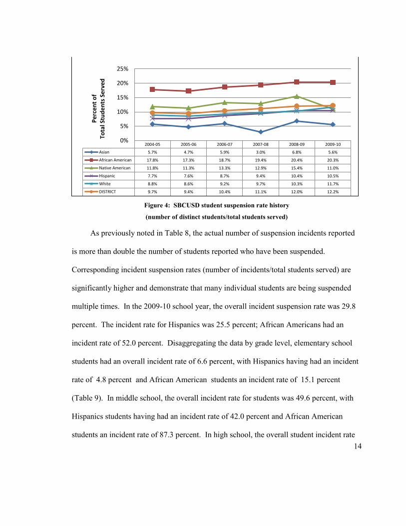
Figure 4: SBCUSD student suspension rate history

(number of distinct students/total students served)

As previously noted in Table 8, the actual number of suspension incidents reported

is more than double the number of students reported who have been suspended.

Corresponding incident suspension rates (number of incidents/total students served) are

significantly higher and demonstrate that many individual students are being suspended

multiple times. In the 2009-10 school year, the overall incident suspension rate was 29.8

percent. The incident rate for Hispanics was 25.5 percent; African Americans had an

incident rate of 52.0 percent. Disaggregating the data by grade level, elementary school

students had an overall incident rate of 6.6 percent, with Hispanics having had an incident

rate of 4.8 percent and African American students an incident rate of 15.1 percent

(Table 9). In middle school, the overall incident rate for students was 49.6 percent, with

Hispanics students having had an incident rate of 42.0 percent and African American

students an incident rate of 87.3 percent. In high school, the overall student incident rate

2004-05 2005-06 2006-07 2007-08 2008-09 2009-10

Asian 5.7% 4.7% 5.9% 3.0% 6.8% 5.6%

African American 17.8% 17.3% 18.7% 19.4% 20.4% 20.3%

Native American 11.8% 11.3% 13.3% 12.9% 15.4% 11.0%

Hispanic 7.7% 7.6% 8.7% 9.4% 10.4% 10.5%

White 8.8% 8.6% 9.2% 9.7% 10.3% 11.7%

DISTRICT 9.7% 9.4% 10.4% 11.1% 12.0% 12.2%

0%

5%

10%

15%

20%

25%

Pe

rce

nt

of

To

tal S

tud

en

ts S

erv

ed

15

was 58.9 percent, with Hispanic students having a rate of 53.6 percent and African

American students an incident rate of 91.9 percent.

Table 9: SBCUSD 2009-10 suspension incident rates by level and ethnicity

Ethnicity Group

Student Level All Students African American Hispanic White

Elementary School 6.6% 15.1% 4.8% 7.3%

Middle School 49.6% 87.3% 42.0% 44.8%

High School 58.9% 91.9% 53.6% 49.2%

All Schools 29.8% 52.0% 25.5% 27.8%

One significant finding of the suspension analysis by SBCUSD has been that student

suspensions in the period between the sixth and ninth grades account for more than half of

the total suspension incidents in any given school year. Figure 5 summarizes suspension

incidents by grade. In 2009-10, for example, the reported grade 8 incident suspension

rate of 62.5 percent indicates that the total number of grade 8 incident suspensions is equal

to 62.5 percent of the October CBEDS census enrollment, approximately 2,673 incidents.

Figure 5: SBCUSD incident rates by CBEDS grade

(number of suspension incidents/reported CBEDS enrollment by grade)

K 1 2 3 4 5 6 7 8 9 10 11 12

2004-05 0.5% 2.4% 3.9% 6.7% 11.0% 13.9% 26.7% 38.8% 47.4% 62.9% 33.6% 15.6% 10.8%

2005-06 0.1% 1.5% 2.2% 4.9% 8.9% 12.3% 27.2% 40.3% 51.8% 53.8% 31.1% 18.1% 9.9%

2006-07 0.3% 1.1% 2.6% 4.1% 5.1% 9.6% 16.0% 33.7% 47.0% 85.6% 35.0% 18.9% 11.5%

2007-08 1.0% 3.1% 4.2% 4.8% 8.9% 10.1% 35.0% 55.3% 66.9% 72.5% 27.2% 14.9% 13.3%

2008-09 1.2% 3.6% 5.1% 6.5% 12.2% 15.0% 29.5% 56.7% 64.3% 77.1% 70.1% 45.3% 18.3%

2009-10 1.6% 3.3% 3.8% 7.8% 11.3% 13.2% 30.5% 45.1% 62.5% 107.2% 79.6% 45.6% 18.4%

0%

20%

40%

60%

80%

100%

120%

Pe

rce

nt

of

En

rollm

en

t

16

The rate of suspension incidents is observed to peak at grade 9 (Figure 5). An

extreme peak is reported in 2009-10 for grade 9 with an incident suspension rate of 107.2

percent. This indicates that the total number of grade 9 suspension incidents (4,191

incidents) is greater than the reported CBEDS enrollment at grade 9 (3,911 students) by

slightly more than seven percent.

Research within SBCUSD has focused on a number of factors to help explain the

increase in suspension incidents between grades 6 and 9. In grade 6, students are

transitioning from elementary school to middle school. In grade 9, the students have to

transition again to high school. District performance indicators such as standardized test

scores, course grades, attendance and dropouts as well as discipline records indicate that

many of these suspended students are struggling. The suspension gap between significant

groups of SBCUSD students by ethnicity has yet to be adequately explained by these

factors alone.

1.3 Organization of Thesis

The remainder of the thesis is divided into four chapters. Chapter 2 provides relevant

background information. Chapter 3 reviews the methods and data sources used in the hot spot

analysis and regression analysis while chapter 4 presents the results of the analysis. Chapter 5

summarizes the major findings, considers how the results might be used to shape district

administrative policy for reducing the number of out-of-school suspensions, and offers several

conclusions about the results and methodology used in this research.

17

Chapter 2

Literature Review

2.1 Suspensions: Definition and Policies

A suspension, in the context of this study, specifically refers to those out-of-school

suspensions during which a student is excluded from school for disciplinary reasons for

one or more school days (Planty et al. 2009). In the case of extreme behavior,

suspension incidents may result in student expulsions.

While maintaining student discipline has been a long-time problem in schools, it

was not until the mid-1970s that school discipline policies began to receive significant

national focus. In The Epidemic of School Violence, Brodbelt (1978) reviews the

problems of student discipline and school violence and the challenges faced by large urban

districts. Troubled schools were reported as having chronic student discipline problems.

Important factors identified as influencing the problems included middle and high school

aged students from inner-city schools with low socioeconomic status.

Modern suspension policies can be traced back to the United States Supreme Court

case of Goss v. Lopez (419 USC 565 1975), a class action law suit that was brought

against Ohio school officials for suspending students without a hearing. The court held

that the students were denied due process of the law in violation of the 14th

Amendment.

Suspensions of 10 or more days were deemed to require due process procedures.

Suspension of less than 10 days were permissible and required that the student be given

18

oral or written notice of the charges against them. Formal notice and an expulsion hearing

should precede the removal of a student from school.

With the decision of the court in Goss v. Lopez, each state’s education code and

local school district policies began to be revised, codifying the rules under which students

were to be suspended. Typical issues addressed include the prohibition of the use of

alcohol and drugs, violence against students and school staff, and student behavior such as

bullying or hazing.

Analysis of data from a national safe school study by Wu et al. (1982) considered

student misbehavior as well as teacher judgments and attitudes, administrative structures,

effects of perceived academic potential and racial bias. Their conclusion was that

“suspension rates cannot be regarded as a simple reflection of student misbehavior in

school, but rather as the result of a complex of factors grounded in the ways schools

operate.” Research by Bowditch (1993) supports the notion that how a school operates

can influence the suspension rate and details how disciplinarians are reported to use

suspensions “to get rid of troublemakers.”

On a national level, public concerns over safety in schools have also shaped school

policy. A series of school shootings lead to the Gun Free Schools Act (GFSA) of 1994,

20 USC 8921, which requires that all school districts receiving federal education funding

have mandatory one-year expulsion policies in place for students caught bringing a

firearm to school (Feinstein 2010). In response to federal policy, California and many

other states implemented what are now known as Zero Tolerance suspension policies,

19

where any student incident involving weapons or potential weapons would be punished

with an expulsion and a referral to law enforcement (CDE 2009).

While the goal of Zero Tolerance policies is to ensure that the school environment

remains safe for students, these policies have become quite controversial in application at

the district and school level. There are many documented cases where the policy is

misused and minor infractions are given harsh punishments (Skiba et al. 1999; Skiba

2000a; Martin 2001; Martinez 2009). The American Academy of Pediatrics (AAP)

policy statement on suspensions and expulsions expresses concern that such incidents

“may exacerbate academic deterioration, and when students are provided with no

immediate educational alternative, student alienation, delinquency, crime and substance

abuse may ensue” (Taras 2003).

2.2 Who Gets Suspended?

Researchers have identified two important trends over time in the statistics reported by the

US Department of Education National Center for Educational Statistics (NCES) in terms

of who gets suspended from school: (1) males are more likely to be suspended than

females; and (2) minority students, especially African Americans, are more likely to be

suspended than White students (Planty et al. 2009). These official statistics confirm the

results of numerous suspension studies that investigated who was being suspended in US

schools. Many of these studies also indicate that a significant correlation exists between

the rate of student suspensions to grade level and poverty status. Representative studies

that discuss these trends include the following:

20

Tobin et al. (1999) found that frequency of grade 6 suspensions was useful as a

screening device for predicting the frequency of suspensions in grade 9. Referrals for

violence in grade 6 indicated that students were likely to receive referrals for similar

infractions in the future. Boys referred for fighting more than twice and girls for

harassment once in grade 6 were unlikely to be on track for graduation in high school.

Three suspensions in grade 9 predicted school failure.

Mendez et al. (2003) studied how suspensions differed by race and gender in a

large Florida school district. Their findings showed that over-representation of African

American students for suspensions begins in elementary schools. Suspension rates for all

students in all demographic groups increased through elementary and middle school and

dropped off in high school. African Americans, both males and females, had significantly

higher student incident rates (males: 57 incidents per 100 students; females: 27 incidents

per 100 students) than White students (males: 23 incidents per 100 students; females: 8

incidents per 100 students). Disobedience accounted for 20 percent of all incidents.

Arcia (2007) studied some of the student, school and community factors that may

explain the variability in suspension rates within the African American community at the

secondary level. Included in the study were factors measuring academic achievement,

non-African American suspension rates, African American enrollment rates, poverty

measures (free and reduced lunch participation), teacher experience, and teacher race and

gender. Suspensions of African American students were found to significantly correlate to

21

achievement (negatively), years of teacher experience (negatively), an African American

teaching staff (positively) and free and reduced lunch participation (positively) .

Jordan et al. (2009) tested the hypothesis that the odds of a student being referred

for disciplinary action in the middle school setting (8th grade) increases if the student is

male, black, in special education classes, or is poor. They concluded that, with the

exception of students assigned to special education classes, low income students are up to

eight times more likely to be sent for disciplinary referrals than others.

Gregory et al. (2010) in a synthesis of research from over 30 years consider how

the disproportionate suspension of minority students might contribute to the gap in

achievement among racial and ethnic students. In particular, they note that educational

research has shown that a strong link exists for students between time engaged in learning

and achievement. Students with frequent suspensions appear to be at significant risk for

academic underperformance. In addition to race and ethnicity, other factors that appear

related to suspensions include socioeconomic status and neighborhood characteristics for

crime and violence.

2.3 Neighborhoods and Suspensions

Few scholars and practitioners have explored the link between neighborhoods and

suspensions. One immediate challenge involves the delineation of neighborhoods. Two

examples demonstrate the challenges:

Guest and Lee (1984) explore the ways that residents of the Seattle metropolitan

region define "neighborhood" in the abstract and their own neighborhoods in particular.

22

On the whole, the neighborhood is regarded as a relatively limited unit, both in terms of

areal size and functional relevance. Individuals surveyed in the study were found to

define neighborhood in terms of social or spatial factors with variation according to

patterns of local activity, social-demographic characteristics, and the physical

environment. They also differed in their views on its geographic size and institutional

development. While only a small proportion of the variation in responses is explained, the

results suggest that “neighborhood definitions are rational responses to the social and

physical position of the respondent within urban society”.

Tatalovich et al. (2006) examined three methods to define contextual units

(neighborhoods) for a sample of children enrolled in a respiratory health study. The

estimates of contextual variables were found to vary significantly depending on the

method used for choosing neighborhood boundaries and weights. Their conclusion was

that the choice of boundaries therefore shapes the community profile and the relationships

between its variables.

A second challenge is discerning the relationship between neighborhoods and

suspensions from the available literature. Suspensions themselves are generally not

mentioned by the researchers. Much of the relevant research, though informative, focuses

on outcomes that might be classified as a “suspendable” event or stem from the same root

causes, such as juvenile delinquency, the use of alcohol or tobacco by minors, or school

dropouts. Participants in these studies are often characterized simply as “youth” rather

than as students and may in fact be considerably older than high school students.

23

Peeples and Loeber (1994), for example, used census data to classify

neighborhoods as underclass or not underclass. When African American and White youth

were compared without regard to neighborhood, the African Americans were more

frequently and more seriously delinquent than White youth. In those neighborhoods that

were not underclass, African Americans were found to be no more delinquent than White

youth. Overall, ethnicity, single-parent status, and welfare use were not found to be

related to delinquent behavior.

Ennett et al. (1997) measured neighborhood and school characteristics using

student, parent, and archival data. Their findings show substantial variation across schools

in substance use. Lifetime alcohol and cigarette use rates were found higher in schools

located in neighborhoods having greater social advantages as indicated by the perceptions

of residents and archival data.

Leventhal and Brooks-Gun (2000) performed a comprehensive review of

neighborhood residence and the effects on childhood and adolescent well-being. They

found important connections between high socioeconomic status and achievement on the

one hand and low socioeconomic status and residential instability and

behavioral/emotional outcomes on the other hand.

Crowder and South (2003), in their research, focused on whom and under what

conditions do neighborhood characteristics matter most. For African Americans, they

showed that increased socioeconomic distress has resulted in an increase in high school

dropouts, particularly for students in single-parent households. In highly disadvantaged

24

neighborhoods, the risk of dropping out was twice as high for males as for females. For

both African Americans and Whites, their results indicate that the impact of neighborhood

distress on school dropout is stronger for recent in-movers than for long-term residents.

2.4 Social Disorder Theory

If there is a spatial link that explains the relationship between neighborhoods and student

suspensions, it might be found in Social Disorganization Theory (SDT) research. From a

spatial perspective, SDT is one of the most influential explanations for neighborhood

differences in crime and delinquency. The theory focuses on the effects of “kinds of

places”— specifically, different types of neighborhoods—in creating conditions favorable

or unfavorable to crime and delinquency (Kubrin and Weitzer 2003).

With a specific focus on schools, Laub and Lauritsen (1998) have reviewed more

than 60 years of SDT research. They cite three key factors to understanding neighborhood

crime: (1) low socioeconomic status; (2) high population turnover; and (3) racial and

ethnic heterogeneity. These factors impact on the ability of a community to organize and

achieve common goals. Neighborhoods with high levels of these factors are considered

socially disorganized. They are characterized by physical deterioration, large numbers of

rental properties, low levels of home ownership, residents in the low SES group, high

turnover rates, and high percentages of immigrants and ethnic minorities. Social

disorganization leads to lack of connections among neighbors, which in turn discourages

those “guardianship” behaviors important to maintaining a sense of community.

25

Ultimately, neighborhoods send their children to neighborhood schools and this lack of

connection potentially shapes the school environment.

Williams et al. (2002) investigated the academic outcomes of youth in an urban

setting. They collected data on living arrangements, relatives and friends’ religiosity,

exposure to academic success, and neighborhood perceptions in order to assess their

impact on intention of youth in the study to complete school, grade point average (GPA),

and number of suspensions. Their findings indicated that gender, church attendance by

peers, and percentage of relatives completing high school were significant in predicting

positive academic outcomes. Perception of neighborhood deterioration was inversely

related to intention for school completion and GPA. School suspensions were positively

related to perception of neighborhood deterioration.

Cantillon et al. (2003) reviews and extends SDT with a focus on the concept of

Sense of Community (SOC). SOC can be defined by four distinct aspects: membership,

influence, sharing of values with an integration and fulfillment of needs, and a shared

emotional connection. As it relates to schools, their work showed that students who came

from neighborhoods with a high SOC were more likely to participate in school activities

than students from neighborhoods with low SOC. Participation in activities was strongly

correlated to high GPA and academic success.

26

Chapter 3

Methods and Data Sources

This chapter describes the methods and data sources used to perform the spatial analysis

on the study area and identify the location of suspension incident hotspots.

The following multi-step procedure was used to test the previously stated

hypotheses. First, a map of the SBCUSD area was prepared, including map layers

identifying the 2010 US Census Block Groups and layers detailing SBCUSD elementary,

middle, and high school boundaries. Second, a dataset for the study was prepared by

combining a complete K-12 student enrollment dataset from the SBCUSD 2009-10 school

year with a suspension incident summary dataset from the same school year. Third,

student records from the dataset were geocoded, mapped into the district boundaries, and

filtered to define an appropriate study area. Fourth, for all students and for each

significant subgroup to be studied, neighborhood enrollment and suspension incident rate

choropleth maps of the study area were constructed by block group. Fifth, spatial analysis

techniques were applied to identify the degree and location of any neighborhood

suspension incident clustering, thereby confirming or disproving the hypotheses. Sixth,

regression modeling techniques were used in order to predict overall neighborhood

suspension incidents.

27

3.1 Preparation of SBCUSD Map

A map of the SBCUSD area was prepared for this project by combining data from several

sources. First, a set of feature classes with SBCUSD boundaries for district elementary,

middle and high schools was obtained from the SBCUSD Facilities Office (2009).

Second, a TIGER/Line shapefile with the 2010 Census Block Groups for San Bernardino

County was downloaded from the US Census Bureau (2010). Using ArcGIS (Esri 2011a),

these features were projected using the California V FIPS 0405 State Plane Coordinate

System based on the NAD 1983 datum with readjustment using the National Spatial

Reference System (NSRS) of 2007 (Esri 2011b).

SBCUSD itself does not have any formally defined neighborhoods. Several

choices for a neighborhood proxy were considered based on geographic size, human

interactions and institutional development. In terms of size, census block groups are the

smallest reported division in the US Census Bureau’s American Community Survey with

between 600 and 3,000 residents. With the exception of the sparsely inhabited northern

zone, census block groups in SBCUSD are generally less than half a square mile in area.

In terms of human interaction, elementary school boundaries are the smallest district-level

administrative area to which a student in SBCUSD can be assigned. They are generally

recognized throughout the district by name and location.

For the purpose of this thesis, a neighborhood was defined as a collection of census

block groups (in whole or part) organized by elementary school boundaries. Analysis was

performed at the block group level. Summary and reporting was made at the elementary

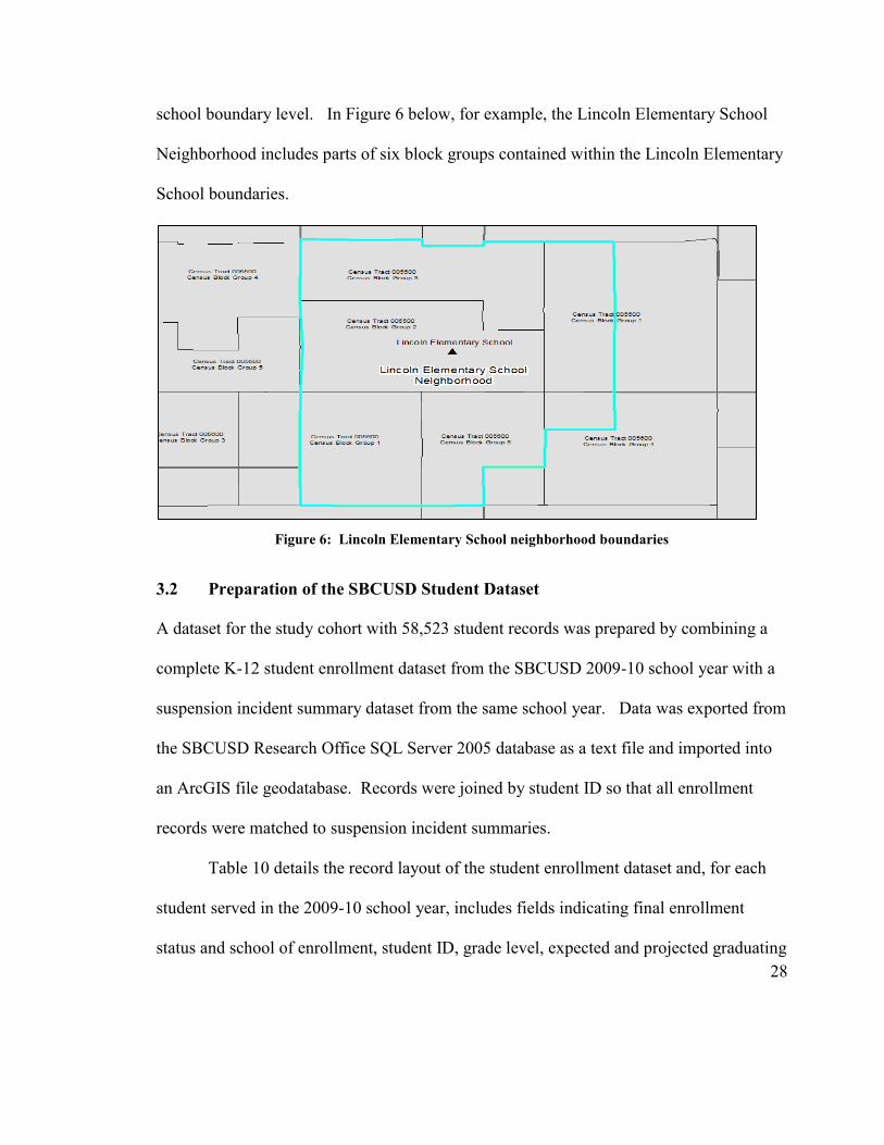
28

school boundary level. In Figure 6 below, for example, the Lincoln Elementary School

Neighborhood includes parts of six block groups contained within the Lincoln Elementary

School boundaries.

Figure 6: Lincoln Elementary School neighborhood boundaries

3.2 Preparation of the SBCUSD Student Dataset

A dataset for the study cohort with 58,523 student records was prepared by combining a

complete K-12 student enrollment dataset from the SBCUSD 2009-10 school year with a

suspension incident summary dataset from the same school year. Data was exported from

the SBCUSD Research Office SQL Server 2005 database as a text file and imported into

an ArcGIS file geodatabase. Records were joined by student ID so that all enrollment

records were matched to suspension incident summaries.

Table 10 details the record layout of the student enrollment dataset and, for each

student served in the 2009-10 school year, includes fields indicating final enrollment

status and school of enrollment, student ID, grade level, expected and projected graduating

29

class (high school only), demographics, socioeconomic status, English learner status and

language proficiency level, and residence address. On export from the student database,

binary counting fields were added to simplify the later summarizing of enrollment.

Table 10: SBCUSD 2009-10 enrollment record layout

For those students who were also present on the October CBEDS Census Day, the

layout included additional fields indicating cumulative grade point average (GPA),

Field Name Data Type Field Description Notes

unique_id Integer unique record id

stu_status_code Text Final Enrollment Status Code

Indicates final enrollment status:

stu_status_description Text Final Enrollment Status Description <<BLANK>> = Enrolled; Drop; Transfer

sch_type Text School Type Elementary, Middle, High

sch_name Text School Name

sch_id Integer School ID

stu_trk Text School Track

stu_id Integer Student Local ID

stu_grade Text Student Grade K - 12

stu_class_of Text Student Class Of ie. 2010

stu_grad_year Text Student Expected Grad Year ie. 2011

stu_sex Text Student Gender M= Male; F = Female

stu_dob Text Student Date of Birth yyyymmdd

stu_ethnicity_code Integer Student Primary Ethnicity Code State codes indicating primary Race and Ethnicity

stu_ethnicity_group_code Integer Student Primary Ethnicity Group Code Ex. 500 = Hispanic, 600 = African American, 700 = White

stu_lowses_status Text Student Socioeconomic Disadvantaged Reported as Yes/No

stu_lep_status Text Student English Learner Type State codes indicating English Learner Type

stu_lang_proficiency_level Text Student English Language Fluency State codes indicating English Language Fluency

stu_residence_address Text Student Residence Address For Geocoding Purposes

stu_residence_city Text

stu_residence_state Text

stu_residence_zip_code Text

stu_residence_zip_plus4 Text

CNT Integer Enrolled 2009-10 1 = Yes; 0 = No

CNT_B Integer African American Enrolled 2009-10 1 = Yes; 0 = No

CNT_H Integer Hispanic Enrolled 2009-10 1 = Yes; 0 = No

CNT_W Integer White Enrolled 2009-10 1 = Yes; 0 = No

CNT_LowSES Integer SED Enrolled 2009-10 1 = Yes; 0 = No

CBEDS_Enrolled Integer Enrolled on CBEDS Day, Oct 2009 1 = Yes; 0 = No

CBEDS_GPA Decimal Overall GPA as of CBEDS Day

CBEDS_ABS Integer Number of Days Absent for 2009-10 on CBEDS Day

CBEDS_sch_elm Integer Enrolled in Elementary School on CBEDS Day 1 = Yes; 0 = No

CBEDS_sch_ms Integer Enrolled in Middle School on CBEDS Day 1 = Yes; 0 = No

CBEDS_sch_hs Integer Enrolled in High School on CBEDS Day 1 = Yes; 0 = No

sx_male Integer Student is Male 1 = Yes; 0 = No

stable_0809 Integer Student was stable in 2008-09 1 = Yes; 0 = No

atrisk_gpa Integer Is CBEDS_GPA < 2.0* 1 = Yes; 0 = No *Select Grades Only

atrisk_abs Integer Is CBEDS_ABS > 4 1 = Yes; 0 = No

atrisk_mob Integer Was student Mobile in 2008-09 1 = Yes; 0 = No

atrisk_1_susp0809 Integer Was student suspended in 2008-09 1 = Yes; 0 = No

atrisk_n_susp0809 Integer Number of suspension incidents in 2008-09

atrisk_days_susp0809 Integer Number of Days Suspended in 2008-09

All Students

CBEDS Enrolled Students Only

30

number of days absent from school as of CBEDS Day, a student stability indicator for the

previous 2008-09 school year, a summary of suspensions from 2008-09, and additional

counting fields for summarizing the CBEDS indicators.

Table 11 details the record layout of the student suspension incident summary and,

for each suspended student in the 2009-10 school year, includes fields indicating student

ID and incident(s) school year, a count of the total number of suspension incidents, a

count of the total number of days suspended, the number of incidents involving drugs and

alcohol, the number of incidents involving violent physical assaults, the number of

expulsions from district schools, and the number of incidents of certain frequently

occurring incident types.

Table 11: SBCUSD 2009-10 suspension incident summary record layout

Field Name Data Type Field Description Notes

stu_id integer Student Local ID

schyear Text School year All Records Marked 2009-10

N_incidents integer Number of Suspension Incidents Total Number of Incidents

N_days_suspended integer Number of Days Suspended Total Number of Days Suspended

N_drug_alcohol_incidents integer Number of Incidents Marked Drugs/Alcohol Includes Incidents marked EC 48915 (a3)/(c3) and

Incidents marked EC 48900 (c )/(d)/(j)

N_violent_incidents integer Number of Incidents Marked as Violent Includes Incidents marked EC 48915 (a1)/(c4)/(a5) and

Incidents marked EC 48900 (a2)/(q)

N_expulsions integer Number of Incidents Indicating Expulsions Incidents indicating Full or Stipulated Expulsion

rsn_k integer Number of EC 48900 (k) Incidents Defiance

rsn_a integer Number of EC 48900 (a) Incidents Attempt to Cause Physical Injury to Another

rsn_i integer Number of EC 48900 (i) Incidents Obscene Act, Profanity or Vulgarity

pds_a1 integer Number of EC 48915 (a1) Incidents Causing Serious Physical Injury to Another

rsn_c integer Number of EC 48900 (c) Incidents Possessed, Used, Sold Controlled Substance/Alcohol

rsn_f integer Number of EC 48900 (f) Incidents Attempt or Causing Damage to School/Private Property

rsn_a2 integer Number of EC 48900 (a2) Incidents Possession of Knife, Explosive or Other Dangerous Object

rsn_p integer Number of EC 48900 (p) Incidents Sexual Harrassment

rsn_b integer Number of EC 48900 (b) Incidents Possessed, Sold, Furnished Firearm, Knife, or Other

Dangerous Object

rsn_r integer Number of EC 48900 (r) Incidents Intentionally Engaged in Harrassment Against Pupil(s) or

Staff

rsn_h integer Number of EC 48900 (h) Incidents Possessed or Used Tobacco or Tobacco Products

pds_a2 integer Number of EC 48915 (a2) Incidents Possession of Knife, Explosive or Other Dangerous Object

of No Reasonable Use to the Student

rsn_g integer Number of EC 48900 (g) Incidents Stole/Attempted to Steal School/Private Property

rsn_j integer Number of EC 48900 (j) Incidents Possessed, Offered, Arranged or Negotiated to Sell Drug

Paraphernalia

2009-10 Suspended Students Only

2009-10 Suspension Incident Summary

2009-10 Frequency of Select Incidents

31

3.3 Geocoding the Dataset and Defining an Appropriate Study Area

The student data prepared in Section 3.2 included primary residence address. The data

were geocoded using the geocoding tools available in ArcGIS and added as a point feature

class into the map prepared in Section 3.1.

Previous analysis by the SBCUSD Research Office indicated that a small number

of students, less than 0.5 percent of the total enrollment served, lived outside the regular

district boundaries or in the sparsely populated northern margins of the district. In order

to avoid skewing the proposed analysis, these students were identified and excluded from

the study cohort. The final 58,246 student records remaining in the dataset represent

slightly more than 99.5 percent of the total student enrollment served in the 2009-10

school year. Of the 7,119 unique students who were suspended in SBCUSD over the

same period, the study cohort was found to include 7,043 of the students, more than 98.9

percent of those students suspended.

Once the final student cohort was identified, a study area for the analysis was

defined that bounded the point feature class of the filtered student cohort. Student

residences were observed to run from the northwest to the southeast and were roughly

bounded by a triangle formed by the San Bernardino Mountains to the north, the Santa

Ana River to the southeast, and Interstate 215 along the west. An ArcGIS extension, X-

Tools Pro (DataEast 2011), was used to generate a convex hull, a minimal bounding

polygon, containing all the points of the feature set (Buckley 2008). As a final step, in

order to reduce the risk of edge effects in the planned analysis, a 3,000 foot buffer was

32

applied to the convex hull. Elementary school boundaries and census block group feature

class layers were clipped to the study area. The final study area showing school locations

and clipped census block groups is shown in Figure 7.

Figure 7: SBCUSD suspension study area

3.4 Visualizing SBCUSD Enrollment and Suspension Incident Rates

SBCUSD enrollment and suspension incidents were summarized by census block group

and by elementary school neighborhood. In order to identify any resultant patterns, the

data was visualized using choropleth maps.

33

First, a spatial join was performed matching the attributes of the geocoded student

cohort prepared in Section 3.3 to the clipped census block groups. For each block group,

the spatial join summarized the integer fields detailed in Tables 10 and 11, including total

enrollment served, number of suspension incidents, and number of suspensions by

incident type.

In a similar manner, using select subgroups of the geocoded student cohort, spatial

joins were performed summarizing enrollment and suspensions by significant SBCUSD

ethnicities (African American, Hispanic, White) and socioeconomic disadvantaged status.

The resultant polygon feature classes were used to prepare choropleth maps

visualizing enrollment numbers and suspension incident rates for all students, significant

ethnic subgroups of students, socioeconomically disadvantaged students and those

students with primary suspension incidents indicating defiance, drug and alcohol use, and

violent acts. For the purpose of this thesis, suspension incident rates were defined as the

number of suspension incidents in a given block group divided by the total number of

students served within the block group. The final prepared maps used seven classes to

visualize enrollment and incidents, with the classification scheme determined for each

map using a Jenks Natural Breaks methodology.

The same basic procedure was repeated in order to match students to elementary

school neighborhoods and prepare neighborhood summary tables of enrollment and

suspension incidents. This step was taken as a cross-check to ensure that enrollment and

suspension incident counts totals closely matched the expected totals for the district.

34

3.5 Spatial Analysis of the SBCUSD Suspension Incidents

Spatial analysis techniques were applied to the polygon feature classes prepared in Section

3.4 in order to identify the degree and location of any neighborhood suspension incident

clustering, thereby confirming or disproving the thesis hypotheses.

3.5.1 Measuring Spatial Autocorrelation using Moran’s Global I

As an initial test to disprove the hypotheses, Moran’s Global I was used to determine the

degree of spatial autocorrelation of suspension incidents within the study area census

block group features for all students and subgroups. Moran’s Global I is a ratio that

compares the difference in values of neighboring features to the difference in values

between all features in the study area. In the numerator, for each pair of neighboring

features, the mean value for all features in the study area is subtracted from the value of

each feature and its neighbor and the product of these differences is calculated and

multiplied by the weight for that pair and then summed. In the denominator, the variance

from the mean value for all pairs is calculated and multiplied by the sum of all weights.

The complete formula for determining the statistic is shown in Equation (1) below

(Mitchell 2009):

where I measures the spatial autocorrelation of x in each i and j neighboring features with

spatial weight w in the study area having a total of n features.

∑ ∑ ( ̅)( ̅)

∑ ∑ ∑ ( ̅)

(1)

35

In a random distribution, Moran’s Global I will be close to 0 because there will be

nearly the same number of positive products summed with negative products in the

numerator. In a clustered distribution, where neighboring features are more similar,

Moran’s Global I will be greater than 0 because the overall sum of products in the

numerator will be positive. In a dispersed distribution, where neighboring features are

dissimilar, Moran’s Global I will be less than 0 because the sum of products in the

numerator will be negative. As implemented within ArcGIS, along with the Moran’s

Global I statistic, the statistic is compared to its expected value and a normally distributed

Z-score is produced to indicate the likelihood that the clustering pattern is due to chance.

A key component to the planned hot-spot analysis was determining the

neighborhood distance band where influence of incidents upon clustering is most

pronounced. To do this, an incremental spatial autocorrelation analysis of the study area

suspension incidents by census block groups was made where Moran’s Global I was

calculated for a neighborhood distance band beginning at 1,000 feet and then repeated

incrementally with neighborhood size increasing by 500 feet. Reported Z-scores were

recorded and graphed as a function of distance. A peak in Z-scores indicates the distance

where clustering is significant. For all students and subgroups, a distance band was

identified where Z-scores indicated effects upon clustering were most pronounced. In

Figure 8 below, for example, Z-scores for Moran’s Global I were calculated for

suspension incidents classified as defiance (EC 48900(k)) and graphed at varying

distances. Peaks in the graph at 1,500 feet, 5,000 feet, and 6,500 feet indicate significant

36

distance bands for clustering. Clustering was determined to be most pronounced at a

distance of 6,500 feet.

Figure 8: Moran's Global I for suspensions incidents classified as defiance - EC 48900(k)

3.5.2 Getis-Ord Gi*(d) Hot-Spot Analysis

In order to determine where clustering of suspension incidents occurs within the study

area and estimate its magnitude, a Getis-Ord Gi*(d) Hot-Spot Analysis was performed

within the study area census block features for all students and subgroups. For each

feature in the study area, the Gi*(d) statistic compares the value of neighboring features

within a specified distance (d) and indicates the extent to which each feature is surrounded

by similarly high or low values. The statistic is calculated by summing the value of each

neighbor within a specified distance (where each wij = 1) and dividing by the sum of all

37

neighbor values within the study area. The complete formula for determining the statistic

is shown in the following equation (Mitchell 2009):

where Gi*(d) measures the intensity of clustering of x for each i feature at a distance no

more than d units from neighboring j features with spatial weight w in the study area.

A group of features with high Gi*(d) values indicates a hot-spot or concentrated

clustering of neighboring features with high values. Similarly, a group of features with

low Gi*(d) values indicates a cold-spot or concentrated clustering of neighboring features

with low values. As implemented within ArcGIS, along with the Gi*(d) statistic, the

statistic is compared to its expected value and a normally distributed Z-score is produced

to indicate the likelihood that the clustering pattern is due to chance.

Using the neighborhood distance bands determined in Section 3.5.1 where the

clustering effects were most pronounced, clusters of suspension incidents for all students

and subgroups were visualized by mapping Gi*(d) Z-scores of census block group

features. Suspension incident hot-spots were identified where census block groups had

Gi*(d) Z-scores greater than 2.58, indicating that the clustering pattern had a less than 1

percent likelihood (p<.01) that the observed pattern was due to random chance.

( )

∑ ( )

∑ (2)

38

3.5.3 Hot-Spot Summary Using Spatial Intersection

In Section 3.5.2, suspension incident hot-spots were identified by census block group. A

programmatic model, depicted below in Figure 9, was built within ArcGIS to summarize

and report the results of the hot-spot analysis as a percentage of the elementary school

neighborhoods with census block groups having Gi*(d) incident clustering with a Z-score

greater than 2.58 (p<0.01).

Figure 9: Hot-spot summary model using spatial intersection

For all students and each subgroup analyzed for hot-spots, the model automated

the following steps: (1) select those census block groups having Gi*(d) analysis results

with a Z-score greater than 2.58; (2) perform a spatial intersection between the

elementary school neighborhoods defined in Section 3.1 and the selected census block

groups; (3) summarize the results of the spatial intersection within the neighborhood as

both a count of intersected census block groups and the sum of the total area of the census

block groups; and (4) output the results as a DBF file. The final DBF file was prepared

39

by joining each of the DBFs to a master list of elementary school neighborhoods. For all

students and each significant subgroup, a table was prepared reporting the percentage of

each elementary school neighborhood having Gi*(d) incident clustering with a Z-score

greater than 2.58 (p<0.01).

3.5.4 Neighborhood Hot-Spot Grouping Patterns

As a final step in the hot-spot analysis, the table prepared in Section 3.5.3 detailing

suspension incident clustering in elementary school neighborhoods was sorted and

organized to identify patterns among the grouped neighborhoods.

Hierarchical clustering software routines were used to order suspension incident

clustering by neighborhood (SAS 2012a). Using this method, each neighborhood starts as

its own cluster. At each step in the process, the two neighborhood clusters that were

closest together by a given distance measure were combined into a single cluster (SAS

2012b). This process was repeated until only a single cluster remained. A dendrogram

was used to visualize the clustered output.

Final grouping of the hierarchically ordered clusters was determined using a focus

on suspension incident clustering within subgroups. Several classes of suspension

incident clustering patterns were identified among the elementary school neighborhoods.

To complete the analysis, a choropleth map and a table organized to show the grouping

patterns were prepared.

40

3.6 Suspension Modeling Using Regression

In order to better understand the relationship between various factors contributing to

student suspensions and to identify those neighborhoods where students are most at risk at

being suspended, a model was developed using regression analysis.

3.6.1 Exploratory Regression Analysis

As a first step in developing a suspension model, an exploratory regression analysis was

performed using the records of those students in the dataset who were identified as present

on CBEDS day. The record layout detailed in Table 10 included attributes that previous

research by the SBCUSD Research Office has shown to be significant indicators of

students at risk including: (1) cumulative grade point average (GPA); (2) number of days

absent from school as of CBEDS Day; (3) a student stability indicator for the previous

2008-09 school year; (4) a summary of suspensions from 2008-09; and (5) additional

counting fields for summarizing student CBEDS day demographic and program

indicators.

In the spatial join procedure described in Section 3.4, these CBEDS attributes were

summarized by census block group. Summary attributes for each census block group

were compared to the total number of census block group suspension incidents recorded in

the 2009-10 school year.

Scatterplot matrices of the results were prepared and used, along with correlation

coefficients, to identify a list of likely candidates as explanatory factors in the model being

developed. Points were colorized according to the rate of suspension incidents within

41

each census block group. Analysis of the scatterplot matrices indicated that several of

these factors showed a cone-shaped scattering of the x-y points characteristic of

heteroscedasticity, indicating that the variance in the relationship between x-y points

increased as the magnitude of the x-y points increased. The scatterplot matrix presented in

Figure 10 was generated as part of this process.

Figure 10: Scatterplot matrix: suspension model factors

As a final step in the review, using the exploratory data analysis module within

ArcGIS, combinations of attributes were used to build and identify candidate regression

models chosen to maximize the explanatory power of the model as measured by the

adjusted R2 value, reduce the redundancy of variables as measured by the Variance

Inflation Factor (VIF), and minimize geographic variation as measured by the Koenker

42

(BP) p-value. Redundant variables and those that, on closer examination, indicated a

vagueness of definition were excluded from the model.

3.6.2 Ordinary Least Squares (OLS) Regression

Once attributes for a candidate suspension model were identified, an ordinary least-

squares (OLS) analysis was performed using a two variable model. In an OLS analysis, a

regression line is fitted to the data by minimizing error as measured by the square of the

differences between the actual and predicted values of the model (residuals). Best

modeling practice as suggested by Mitchell (2009) was used to review and determine if

the model was fully specified. Review of the best fitting OLS regression model output

showed some variation of residuals due to heteroscedasticity and the Jarque-Bera statistic

was significant (p<0.01), confirming that the residuals deviated from a normal

distribution. This indicated that the OLS model was not fully specified and should not be

considered despite the model’s high adjusted R2 value. Using the model’s residuals to

calculate Moran’s I, a Z-score of 7.67 indicated the presence of clustering (p < 0.01) in the

residuals and it was determined that a geographically weighted regression (GWR) model

should be considered.

3.6.3 Geographically Weighted Regression

In a geographically weighted regression (GWR), the model coefficients are allowed to

vary across the study area (Mitchell 2009). Using the GWR module in ArcGIS, the OLS

regression model for predicting the number of suspension incidents developed in Section

3.6.2 was extended. Output from the GWR module produced raster layers for the study

43

area by census block group visualizing how the coefficients were allowed to vary, the

distribution of the GWR model residuals, and a local R2 indicating GWR model fit.

Review of the GWR model indicated an improved fit with residuals more

randomly distributed across the study area. Overall, the adjusted R2 for the model

increased to 0.901387 with local R2 values varying from a low of 0.573631 to a high of

0.999422. Final plots comparing the observed and predicted number of suspension

incidents were prepared.

44

Chapter 4

Results

4.1 Patterns in Student Enrollment

Enrollment by residence in census block groups of the more than 58,000 students served

by SBCUSD in the 2009-10 school year has been visualized in the map displayed in

Figure 11. The district has sparsely inhabited regions along the northern mountains,

southern Santa Ana River basin and in the west along the Cajon Pass (Figure 1).

Figure 11: SBCUSD 2009-10 enrollment by census block groups

There are regions within the city where highly populated census block groups,

each having more than 700 students in residence, are interspersed with regions where

fewer than 200 students are in residence within a census block group. This can be

45

explained by observing the many apartment complexes and subdivisions that coexist

alongside land used for industrial warehouses, farming, or left as empty lots. San

Bernardino International Airport (SBX) in the southern portion of the district was once the

site of Norton Air Force Base. In an effort to reduce neighborhood blight, base housing

was razed in the late 1990s and the land has stood empty since that time.

Analysis of the 2009-10 school year enrollment by elementary school

neighborhood shows that enrollment varies greatly across the city. In Table 12 below,

enrollment within the district has been summarized for all students and by significant

subgroup in each elementary school neighborhood. Records are sorted by decreasing total

enrollment. The final column of the table indicates enrollment density per square mile. It

can be easily seen that the Emmerton-Rodriguez neighborhood (N = 2,594 students;

density = 1,942 students/sq. mile), while having the highest number of enrolled students,

has an enrollment density much less than that of other smaller urban neighborhoods such

as Lincoln (N = 1,839 students; density = 3,444 students/sq. mile). In the north of the city,

the Kimbark neighborhood (N = 329 students; density = 21 students/sq. mile) is the least

populated and has the largest areal size (15.48 sq. miles).

Neighborhoods were found to vary by subgroup as well. Hispanic student

enrollment by neighborhood averaged 67.1 percent and ranged from 29.8 percent to 91.9

percent. African American student enrollment by neighborhood averaged 16.7 percent

with a minimum of 3 percent and a maximum of 31.9 percent.

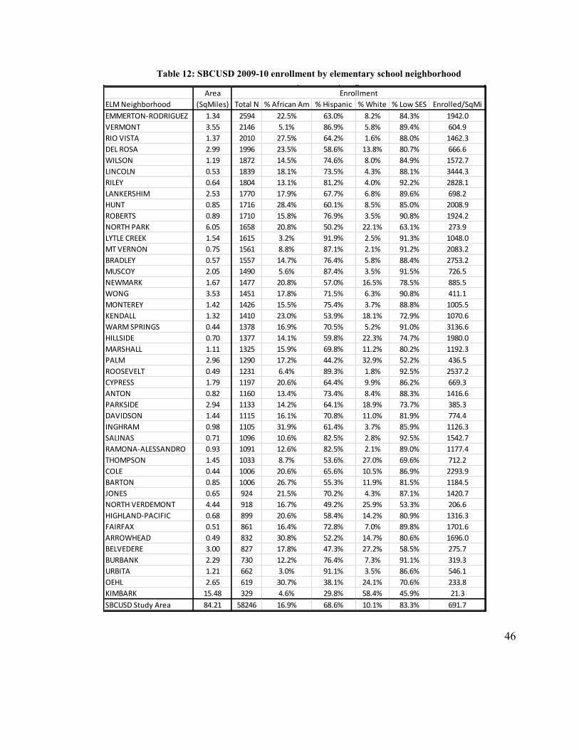
46

Table 12: SBCUSD 2009-10 enrollment by elementary school neighborhood

Area

ELM Neighborhood (SqMiles) Total N % African Am % Hispanic % White % Low SES Enrolled/SqMi

EMMERTON-RODRIGUEZ 1.34 2594 22.5% 63.0% 8.2% 84.3% 1942.0

VERMONT 3.55 2146 5.1% 86.9% 5.8% 89.4% 604.9

RIO VISTA 1.37 2010 27.5% 64.2% 1.6% 88.0% 1462.3

DEL ROSA 2.99 1996 23.5% 58.6% 13.8% 80.7% 666.6

WILSON 1.19 1872 14.5% 74.6% 8.0% 84.9% 1572.7

LINCOLN 0.53 1839 18.1% 73.5% 4.3% 88.1% 3444.3

RILEY 0.64 1804 13.1% 81.2% 4.0% 92.2% 2828.1

LANKERSHIM 2.53 1770 17.9% 67.7% 6.8% 89.6% 698.2

HUNT 0.85 1716 28.4% 60.1% 8.5% 85.0% 2008.9

ROBERTS 0.89 1710 15.8% 76.9% 3.5% 90.8% 1924.2

NORTH PARK 6.05 1658 20.8% 50.2% 22.1% 63.1% 273.9

LYTLE CREEK 1.54 1615 3.2% 91.9% 2.5% 91.3% 1048.0

MT VERNON 0.75 1561 8.8% 87.1% 2.1% 91.2% 2083.2

BRADLEY 0.57 1557 14.7% 76.4% 5.8% 88.4% 2753.2

MUSCOY 2.05 1490 5.6% 87.4% 3.5% 91.5% 726.5

NEWMARK 1.67 1477 20.8% 57.0% 16.5% 78.5% 885.5

WONG 3.53 1451 17.8% 71.5% 6.3% 90.8% 411.1

MONTEREY 1.42 1426 15.5% 75.4% 3.7% 88.8% 1005.5

KENDALL 1.32 1410 23.0% 53.9% 18.1% 72.9% 1070.6

WARM SPRINGS 0.44 1378 16.9% 70.5% 5.2% 91.0% 3136.6

HILLSIDE 0.70 1377 14.1% 59.8% 22.3% 74.7% 1980.0

MARSHALL 1.11 1325 15.9% 69.8% 11.2% 80.2% 1192.3

PALM 2.96 1290 17.2% 44.2% 32.9% 52.2% 436.5

ROOSEVELT 0.49 1231 6.4% 89.3% 1.8% 92.5% 2537.2

CYPRESS 1.79 1197 20.6% 64.4% 9.9% 86.2% 669.3

ANTON 0.82 1160 13.4% 73.4% 8.4% 88.3% 1416.6

PARKSIDE 2.94 1133 14.2% 64.1% 18.9% 73.7% 385.3

DAVIDSON 1.44 1115 16.1% 70.8% 11.0% 81.9% 774.4

INGHRAM 0.98 1105 31.9% 61.4% 3.7% 85.9% 1126.3

SALINAS 0.71 1096 10.6% 82.5% 2.8% 92.5% 1542.7

RAMONA-ALESSANDRO 0.93 1091 12.6% 82.5% 2.1% 89.0% 1177.4

THOMPSON 1.45 1033 8.7% 53.6% 27.0% 69.6% 712.2

COLE 0.44 1006 20.6% 65.6% 10.5% 86.9% 2293.9

BARTON 0.85 1006 26.7% 55.3% 11.9% 81.5% 1184.5

JONES 0.65 924 21.5% 70.2% 4.3% 87.1% 1420.7

NORTH VERDEMONT 4.44 918 16.7% 49.2% 25.9% 53.3% 206.6

HIGHLAND-PACIFIC 0.68 899 20.6% 58.4% 14.2% 80.9% 1316.3

FAIRFAX 0.51 861 16.4% 72.8% 7.0% 89.8% 1701.6

ARROWHEAD 0.49 832 30.8% 52.2% 14.7% 80.6% 1696.0

BELVEDERE 3.00 827 17.8% 47.3% 27.2% 58.5% 275.7

BURBANK 2.29 730 12.2% 76.4% 7.3% 91.1% 319.3

URBITA 1.21 662 3.0% 91.1% 3.5% 86.6% 546.1

OEHL 2.65 619 30.7% 38.1% 24.1% 70.6% 233.8

KIMBARK 15.48 329 4.6% 29.8% 58.4% 45.9% 21.3

SBCUSD Study Area 84.21 58246 16.9% 68.6% 10.1% 83.3% 691.7

Enrollment

SBCUSD 2009-10 Enrollment by Elementary Neighborhood

47

White student enrollment averaged 11.6 percent and ranged from 1.6 percent to 58.4

percent. Students identified as having a low socioeconomic status (LowSES) had an

average neighborhood enrollment of 81.8 percent with a minimum of 45.9 percent and a

maximum of 92.5 percent.

Analysis of distribution patterns of student residence by subgroup using a one

standard deviation distribution ellipse (Figure 12 below) shows no discernible pattern with

the exception of the White subgroup. Most student subgroups in the city live inter-mixed

in the southern and central regions of the city. White student residences show a slight

variation with more of these students living along the mountains in the northern edge of

the district. This area includes the more affluent neighborhoods of the city.

Figure 12: Enrollment by subgroup - 1 standard deviation distribution from center

48

4.2 Analysis of Student Suspensions

Student suspensions incidents were found to have the highest rate of occurrence in the

south-central portion of the district in the census blocks located in the downtown region of

San Bernardino City. In Figure 13 below, the red colored census block groups in the

center of study area indicate that more than 50 suspension incidents are occurring per 100

students.

Figure 13: SBCUSD 2009-10 incident rate by census block groups

Comparing the enrollment by census block group map in Figure 11 to the

suspension incident rate map shows only a partial correspondence of high enrollment to

high rates of suspensions. Enrolled students living along the western edge of the district

49

have a much lower rate of suspensions than those students with residences in census block

groups with similar enrollment numbers near the central portion of the district.

4.2.1 Spatial Autocorrelation of Suspension Incidents

Moran’s Global I was used to measure spatial autocorrelation of suspension incidents for

all students and significant subgroups at various distance bands. Results were normalized

and expressed as Z-scores with a mean of 0 and standard deviation of 1. Distance bands

with Z-scores greater than 2.58 indicate significant positive spatial autocorrelation of

suspension incidents (p<0.01), thus disproving the null hypotheses. Table 13 details

those distance bands where Moran’s Global I peaked.

Table 13: Distance bands with most significant clustering of suspension incidents by subgroup

Study Group Distance Band (Feet) Moran’s Global I

Z-score

All Students 6,500 8.44

African American 7,000 8.46

Hispanic 6,500 7.90

White 5,000 6.33

Low Socioeconomic 5,000 8.12

Defiance Suspensions 6,500 8.68

Violence Suspensions 7,500 7.32

Drugs/Alcohol Suspensions 6,000 5.63

4.2.2 Hot Spot Analysis of Suspensions – Detailed Example and Summary

Having determined that suspension clustering within the district does exist, those census

block groups where suspension incident clustering was most pronounced were identified

using Hot Spot Analysis. The Getis-Ord Gi*(d) statistic was calculated for all students

and significant subgroups using the distance bands indicated in Table 13. As described in

50

Section 3.5.2, incident clustering Z-scores were determined for each census block group.

A Z-score greater than 2.58 indicates significant incident clustering (p<0.01) and was

identified as a suspension hotspot.

In Figure 14 below, a portion of the analysis of those suspension incidents

identified as Acts of Violence has been visualized. As defined in Section 3.1, census

block groups within an elementary school’s boundaries are defined to be an elementary

school neighborhood. All census block groups within the Anton Elementary School

neighborhood are shown as red hotspots, having Z-scores greater than 2.58; less than 20

percent of the census block groups within the boundaries of Monterey Elementary School

neighborhood are identified as hotspots.

Figure 14: Hotspot analysis by census block groups using Getis-Ord Gi* statistic

(reported as violence incident clustering z-scores)

51

The visualization of the Lincoln Elementary School neighborhood, having some

census block groups with a positive Z-score less than 2.58, indicates that while some

clustering of violent incidents can be identified, it has no census block groups that are

considered to indicate a hotspot for violent suspension incidents.

Table 14 below summarizes this hotspot analysis and indicates the percent of those

neighborhoods by each suspension incident type studied that are considered to be hotspots.

The table is ordered by hotspot rates for all students and helps to highlight the differences

between neighborhoods. For example, the Warm Springs neighborhood is considered to

be a 100 percent hotspot for all groups analyzed except those focusing on Whites and

Drug/Alcohol suspension incidents. The Emmerton-Rodriguez and Bradley

neighborhoods have high hotspot rates for suspensions involving African Americans

students and much lower rates for suspensions involving Hispanics. Conversely, the

Lincoln neighborhood has a high hotspot rate for suspensions involving Hispanics and

much lower rates for African Americans. The Hillside neighborhood has a high hotspot

rate only for suspensions incidents involving White students.

52

Table 14: Percent of neighborhood hotspot incident clustering by

elementary school neighborhood and suspension incident category

Elementary School Neighborhood Area (sqMiles)All

Students

African

American Hispanic White Low SES Defiance Violence

Drugs

Alcohol

WARM SPRINGS 0.44 100.0% 100.0% 100.0% 0.0% 100.0% 100.0% 100.0% 0.0%

EMMERTON-RODRIGUEZ 1.34 100.0% 100.0% 14.2% 0.0% 77.2% 100.0% 64.7% 23.9%

LINCOLN 0.53 99.9% 0.0% 100.0% 0.0% 100.0% 100.0% 0.0% 74.8%

BRADLEY 0.57 87.1% 15.8% 100.0% 0.0% 99.7% 100.0% 15.9% 19.6%

ANTON 0.82 72.9% 53.2% 70.1% 0.0% 15.9% 72.9% 100.0% 13.0%

ROBERTS 0.89 71.3% 0.0% 99.9% 0.0% 51.4% 99.9% 48.5% 1.8%

FAIRFAX 0.51 57.7% 100.0% 7.8% 0.0% 57.7% 57.7% 100.0% 0.0%

RILEY 0.64 56.3% 0.0% 96.3% 0.0% 46.4% 62.3% 0.0% 56.2%

COLE 0.44 55.1% 55.1% 0.0% 0.0% 55.1% 55.1% 0.0% 0.0%

LANKERSHIM 2.53 38.2% 38.2% 24.0% 0.0% 34.4% 38.2% 24.0% 0.0%

WONG 3.53 30.9% 22.9% 30.9% 0.0% 22.9% 30.9% 30.9% 0.0%

CYPRESS 1.79 22.6% 8.6% 0.0% 0.0% 0.0% 22.6% 0.0% 0.0%

HIGHLAND-PACIFIC 0.68 12.5% 12.6% 0.0% 0.0% 4.1% 12.5% 0.0% 0.0%

JONES 0.65 9.7% 0.0% 89.9% 0.0% 12.9% 42.5% 0.0% 11.3%

MONTEREY 1.42 2.4% 2.4% 2.4% 0.0% 2.4% 2.4% 20.2% 0.0%

WILSON 1.19 2.3% 0.0% 23.1% 0.0% 16.4% 16.4% 6.0% 0.0%

BARTON 0.85 0.1% 99.8% 0.0% 0.0% 0.1% 0.1% 25.8% 0.0%

HUNT 0.85 0.0% 51.2% 0.0% 0.0% 29.1% 0.0% 76.6% 0.0%

ARROWHEAD 0.49 0.0% 0.0% 0.0% 10.3% 0.0% 0.0% 0.0% 0.0%

BELVEDERE 3.00 0.0% 12.7% 0.0% 0.0% 0.0% 0.0% 0.0% 0.0%

BURBANK 2.29 0.0% 0.0% 1.5% 0.0% 0.0% 0.0% 0.0% 0.0%

DAVIDSON 1.44 0.0% 0.0% 0.1% 0.0% 0.0% 0.0% 0.0% 0.0%

DEL ROSA 2.99 0.0% 4.7% 0.0% 0.0% 0.0% 0.0% 0.0% 0.0%

HILLSIDE 0.70 0.0% 0.0% 0.0% 98.2% 0.0% 0.0% 0.0% 0.0%

INGHRAM 0.98 0.0% 0.0% 0.0% 0.0% 0.0% 0.0% 0.0% 38.6%

KENDALL 1.32 0.0% 0.0% 0.0% 39.7% 0.0% 0.0% 0.0% 0.0%

KIMBARK 15.48 0.0% 0.0% 0.0% 0.0% 0.0% 0.0% 0.0% 0.0%

LYTLE CREEK 1.54 0.0% 0.0% 0.0% 0.0% 0.0% 0.0% 0.0% 0.0%

MARSHALL 1.11 0.0% 0.0% 0.0% 0.0% 0.0% 0.0% 0.0% 0.0%

MT VERNON 0.75 0.0% 0.0% 23.9% 0.0% 0.0% 0.0% 0.0% 42.7%

MUSCOY 2.05 0.0% 0.0% 0.0% 0.0% 0.0% 0.0% 0.0% 57.6%

NEWMARK 1.67 0.0% 0.0% 0.0% 3.9% 0.0% 0.0% 0.0% 0.0%

NORTH PARK 6.05 0.0% 0.0% 0.0% 3.3% 0.0% 0.0% 0.0% 0.0%

NORTH VERDEMONT 4.44 0.0% 0.0% 0.0% 0.2% 0.0% 0.0% 0.0% 0.0%

OEHL 2.65 0.0% 0.0% 0.0% 0.0% 0.0% 0.0% 0.0% 0.0%

PALM 2.96 0.0% 0.0% 0.0% 0.0% 0.0% 0.0% 0.0% 0.0%

PARKSIDE 2.94 0.0% 0.0% 0.0% 4.5% 0.0% 0.0% 0.0% 0.0%

RAMONA-ALESSANDRO 0.93 0.0% 0.0% 0.0% 0.0% 0.0% 0.0% 0.0% 0.1%

RIO VISTA 1.37 0.0% 0.0% 0.0% 0.0% 0.0% 0.0% 0.0% 16.9%

ROOSEVELT 0.49 0.0% 0.0% 0.0% 0.0% 0.0% 0.0% 0.0% 0.0%

SALINAS 0.71 0.0% 0.0% 0.0% 0.0% 0.0% 0.0% 0.0% 0.1%

THOMPSON 1.45 0.0% 0.0% 0.0% 0.0% 0.0% 0.0% 0.0% 0.0%

URBITA 1.21 0.0% 0.0% 0.0% 0.0% 0.0% 0.0% 0.0% 0.0%

VERMONT 3.55 0.0% 0.0% 0.0% 0.0% 0.0% 0.0% 0.0% 18.6%

Percent of Incident Clustering within Elementary Neighborhoods with Z-score > 2.58 (p<0.01)

Suspension Incident Category

53

4.2.3 Neighborhood Hot Spot Grouping Patterns

Several classes of incident clustering patterns within neighborhoods were identified in the

table of ordered suspension incident clusters prepared in Section 3.5.4. They include

neighborhoods where: (1) incident clustering is significant for all students and balanced

between African American and Hispanic subgroups; (2) incident clustering is significant

for all students and one ethnic/racial subgroup; (3) incident clustering is not significant for

all students but was significant for one ethnic/racial subgroup; (4) incident clustering is

significant only for drug/alcohol incidents; and (5) incident clustering is not significant.

Elementary school neighborhoods in group 1 (Table 15) generally have the

greatest percent of suspension incident clustering among all neighborhoods and have a

near equal balance of suspension incident clustering between the African American and

Hispanic subgroups. These neighborhoods are also characterized by higher rates of

clustering for the LowSES, violence, and defiance subgroups. The choropleth map in

Figure 15 shows this group in red, extending as a single continuous field across the south-

eastern portion of the study area.

Table 15: Elementary school neighborhoods – group pattern 1

Percent of Neighborhood Hotspot Incident Clustering

Grouping All African Drugs

Pattern Elementary School Neighborhood Area (sqMiles) Students American Hispanic White Low SES Defiance Violence Alcohol

Group 1

WARM SPRINGS 0.44 100.0% 100.0% 100.0% 0.0% 100.0% 100.0% 100.0% 0.0%

ANTON 0.82 72.9% 53.2% 70.1% 0.0% 15.9% 72.9% 100.0% 13.0%

LANKERSHIM 2.53 38.2% 38.2% 24.0% 0.0% 34.4% 38.2% 24.0% 0.0%

WONG 3.53 30.9% 22.9% 30.9% 0.0% 22.9% 30.9% 30.9% 0.0%

MONTEREY 1.42 2.4% 2.4% 2.4% 0.0% 2.4% 2.4% 20.2% 0.0%


Balanced - Similar Clustering for All Students, African

American and Hispanic Subgroups

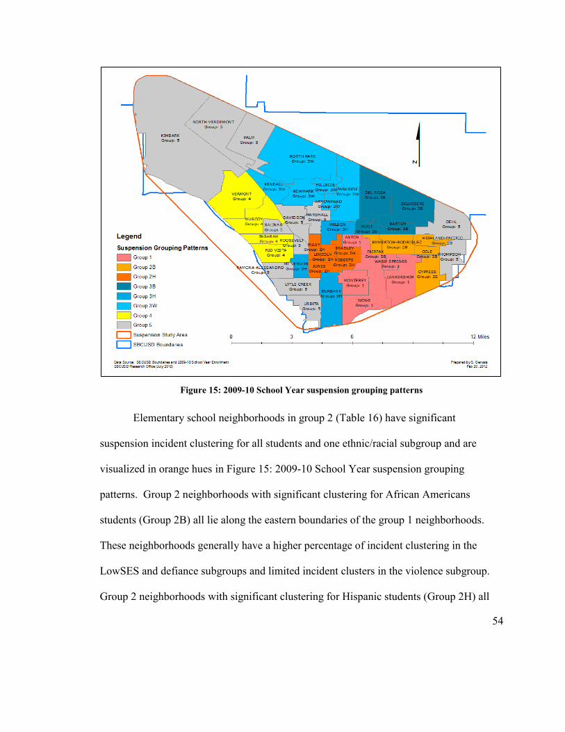
54

Figure 15: 2009-10 School Year suspension grouping patterns

Elementary school neighborhoods in group 2 (Table 16) have significant

suspension incident clustering for all students and one ethnic/racial subgroup and are

visualized in orange hues in Figure 15: 2009-10 School Year suspension grouping

patterns. Group 2 neighborhoods with significant clustering for African Americans

students (Group 2B) all lie along the eastern boundaries of the group 1 neighborhoods.

These neighborhoods generally have a higher percentage of incident clustering in the

LowSES and defiance subgroups and limited incident clusters in the violence subgroup.

Group 2 neighborhoods with significant clustering for Hispanic students (Group 2H) all

55

lie along the northwestern boundaries of the group 1 neighborhoods. These

neighborhoods also have higher percentages of incident clustering in the LowSES and

defiance subgroups. Different from the African American neighborhoods in group 2, the

Hispanic neighborhoods also have higher rates of incident clustering that involve drugs

and alcohol.


In group 3 (Table 17), clustering in elementary school neighborhoods is significant

for only one racial/ethnic group. These neighborhoods generally do not have significant

suspension incident clusters in any other subgroup. Group 3 neighborhoods that have

significant suspension incident clustering for African Americans (Group 3B) lie to the

north along the mountains above the group 2 neighborhoods that have significant incident

clustering for African American students. Group 3 neighborhoods that have significant

incident clustering for Hispanics (Group 3H) are located west of group 1 and north and

south of the group 2 neighborhoods significant for Hispanic incident clustering. Group 3




Group 2

African Am EMMERTON-RODRIGUEZ 1.34 100.0% 100.0% 14.2% 0.0% 77.2% 100.0% 64.7% 23.9%

FAIRFAX 0.51 57.7% 100.0% 7.8% 0.0% 57.7% 57.7% 100.0% 0.0%

COLE 0.44 55.1% 55.1% 0.0% 0.0% 55.1% 55.1% 0.0% 0.0%

HIGHLAND-PACIFIC 0.68 12.5% 12.6% 0.0% 0.0% 4.1% 12.5% 0.0% 0.0%

CYPRESS 1.79 22.6% 8.6% 0.0% 0.0% 0.0% 22.6% 0.0% 0.0%

Hispanic LINCOLN 0.53 99.9% 0.0% 100.0% 0.0% 100.0% 100.0% 0.0% 74.8%

BRADLEY 0.57 87.1% 15.8% 100.0% 0.0% 99.7% 100.0% 15.9% 19.6%

ROBERTS 0.89 71.3% 0.0% 99.9% 0.0% 51.4% 99.9% 48.5% 1.8%

RILEY 0.64 56.3% 0.0% 96.3% 0.0% 46.4% 62.3% 0.0% 56.2%

JONES 0.65 9.7% 0.0% 89.9% 0.0% 12.9% 42.5% 0.0% 11.3%


Clustering High for All Students and Primarily Within One

Race/Ethicity Subgroup

56

neighborhoods that are significant for incident clustering among Whites (Group 3W) lie

near the mountains in the central portion of the city. Neighborhoods in group 3 are

colored in blue hues in Figure 15.


In group 4 (Table 18), clustering for elementary school neighborhoods is

significant for only drug and alcohol suspension incidents. These neighborhoods are all

located along the western edge of the study area and are visualized in Figure 15 using

yellow hues.





Group 3

African Am HUNT 0.85 0.0% 51.2% 0.0% 0.0% 29.1% 0.0% 76.6% 0.0%

BARTON 0.85 0.1% 99.8% 0.0% 0.0% 0.1% 0.1% 25.8% 0.0%

BELVEDERE 3.00 0.0% 12.7% 0.0% 0.0% 0.0% 0.0% 0.0% 0.0%

DEL ROSA 2.99 0.0% 4.7% 0.0% 0.0% 0.0% 0.0% 0.0% 0.0%

Hispanic MT VERNON 0.75 0.0% 0.0% 23.9% 0.0% 0.0% 0.0% 0.0% 42.7%

WILSON 1.19 2.3% 0.0% 23.1% 0.0% 16.4% 16.4% 6.0% 0.0%

BURBANK 2.29 0.0% 0.0% 1.5% 0.0% 0.0% 0.0% 0.0% 0.0%

White HILLSIDE 0.70 0.0% 0.0% 0.0% 98.2% 0.0% 0.0% 0.0% 0.0%

KENDALL 1.32 0.0% 0.0% 0.0% 39.7% 0.0% 0.0% 0.0% 0.0%

ARROWHEAD 0.49 0.0% 0.0% 0.0% 10.3% 0.0% 0.0% 0.0% 0.0%

PARKSIDE 2.94 0.0% 0.0% 0.0% 4.5% 0.0% 0.0% 0.0% 0.0%

NEWMARK 1.67 0.0% 0.0% 0.0% 3.9% 0.0% 0.0% 0.0% 0.0%

NORTH PARK 6.05 0.0% 0.0% 0.0% 3.3% 0.0% 0.0% 0.0% 0.0%


Clustering Low for All Students and High Within One

Race/Ethicity Subgroup




Group 4

MUSCOY 2.05 0.0% 0.0% 0.0% 0.0% 0.0% 0.0% 0.0% 57.6%

INGHRAM 0.98 0.0% 0.0% 0.0% 0.0% 0.0% 0.0% 0.0% 38.6%

RIO VISTA 1.37 0.0% 0.0% 0.0% 0.0% 0.0% 0.0% 0.0% 16.9%

VERMONT 3.55 0.0% 0.0% 0.0% 0.0% 0.0% 0.0% 0.0% 18.6%


Clustering High Only For Drug/Alcohol Incidents

57

Elementary school neighborhoods in group 5 (Table 19) were not identified as

having any significant suspension incident clustering. In Figure 15, they are visualized in

gray and are not located in any specific region of the study area. Neighborhoods in group

5 can be observed near the urban center of the study area and along the less densely

populated edges of the city in the north, south and east.


4.3 Modeling Suspension Incident Rates Using Regression Analysis

Having identified the location for neighborhood suspensions hotspots, a model was

developed using student data gathered during the 2009 October CBEDS data collection to

predict cumulative end-of-school-year suspension incidents by census block group. The

final model was developed in stages using exploratory regression analysis to identify

likely explanatory factors and candidate models, ordinary least-squares regression (OLS)

to refine and validate the candidate model, and geographic weighted regression (GWR) to

account for non-stationary variance in the OLS model.




Group 5

KIMBARK 15.48 0.0% 0.0% 0.0% 0.2% 0.0% 0.0% 0.0% 0.0%

NORTH VERDEMONT 4.44 0.0% 0.0% 0.1% 0.0% 0.0% 0.0% 0.0% 0.0%

PALM 2.96 0.0% 0.0% 0.0% 0.0% 0.0% 0.0% 0.0% 0.1%

OEHL 2.65 0.0% 0.0% 0.0% 0.0% 0.0% 0.0% 0.0% 0.1%

LYTLE CREEK 1.54 0.0% 0.0% 0.0% 0.0% 0.0% 0.0% 0.0% 0.0%

THOMPSON 1.45 0.0% 0.0% 0.0% 0.0% 0.0% 0.0% 0.0% 0.0%

DAVIDSON 1.44 0.0% 0.0% 0.0% 0.0% 0.0% 0.0% 0.0% 0.0%

URBITA 1.21 0.0% 0.0% 0.0% 0.0% 0.0% 0.0% 0.0% 0.0%

MARSHALL 1.11 0.0% 0.0% 0.0% 0.0% 0.0% 0.0% 0.0% 0.0%

RAMONA-ALESSANDRO 0.93 0.0% 0.0% 0.0% 0.0% 0.0% 0.0% 0.0% 0.0%

SALINAS 0.71 0.0% 0.0% 0.0% 0.0% 0.0% 0.0% 0.0% 0.0%

ROOSEVELT 0.49 0.0% 0.0% 0.0% 0.0% 0.0% 0.0% 0.0% 0.0%

No Signif icant Clustering


58

4.3.1 Exploratory Regression Analysis

Exploratory regression analysis identified several possible attributes that could be used in

the candidate suspension model. Table 20 details the summary report of independent

variable significance toward predicting the total number of suspension incidents.

Table 20: Exploratory regression summary of variable significance

CBEDS Enrollment 2009-10 Variable % Significant

N Days Students Suspended 2008-09 100.0%

N Students CBEDS GPA < 2.0 89.7%

N Suspension Incidents 2008-09 81.0%

N LowSES Students 63.1%

N Student Mobile 2008-09 61.0%

Total Days Students Absent At CBEDS 54.1%

N White Students 45.2%

N Male Students 40.4%

N Students CBEDS Absence > 4 39.2%

N Students Suspended 2008-09 30.9%

N Hispanic Students 27.4%

N Students Attending HS 25.5%

N African American Students 19.7%

N Students Attending ELM 18.2%

N Students Attending MS 12.1%

Previous suspensions history from the 2008-09 school year was determined to be

100 percent significant when considered as the total number of days suspended and 81

percent significant when considered as the total number of suspension incidents. The

number of students at-risk of dropping out with a CBEDS reported GPA below 2.0 was

nearly 90 percent significant. Also found significant was the number of students who

59

were in the low socioeconomic (LowSES) subgroup (63%), the number of students who

were mobile (61%), and the number of days of absence logged by CBEDS day during the

2009-10 school year (54%).

4.3.2 Ordinary Least-Square (OLS) Regression

While several combinations of these variables were found to produce suspension models

with good fit, the final analysis indicated that the simplest model with best fit and least

redundancy included only two of the candidate variables: the total number of days

suspended in 2008-09 and the number of students in the LowSES subgroup. The final

OLS model, predicting the number of suspension incidents by census block group, is

given by the equation below:

( ) ( ) ( ) ( )

where for each census block group, i, di = the sum of the number of days suspended in

2008-09 for students living in the ith

census block group; li = the number of identified

LowSES students in the ith

census block group; and S(di,li) = the estimate of the number of

suspension incidents within the ith census block group. Complete output from the OLS

model is reported in Appendix 3.

Overall, the model would appear to be a good predictor of the number of

suspension incidents. The adjusted R2 value for the model was 0.88, indicating that the

model accounts for 88 percent of the variance in the data being modeled. The Wald

statistic indicated that the variables in the model were jointly significant (p < 0.01).

60

Visualizing the standardized residuals of the OLS regression model (Figure 16),

however, indicated that the number of suspension incidents were underestimated on the

west side of the study area and overestimated on the east side of the study area. The

Jarque-Bera statistic was significant (p<0.01), confirming that the residuals deviated from

a normal distribution. The Koenker (BP) statistic was also significant (p < 0.01) and

confirmed that the model has significant non-stationary variance. Using the model’s

residuals to calculate Moran’s I, a Z-score of 7.67 indicated the presence of statistically

significant clustering (p < 0.01) in the residuals and it was determined that a

geographically weighted regression (GWR) model should be considered.

Figure 16: OLS regression model standardized residuals

61

4.3.3 Geographically Weighted Regression

The geographically weighted regression (GWR) model developed in Section 3.6.3

allows the regression coefficients to vary smoothly across the study area. Review of the

GWR model output raster layers indicates an improved fit over the OLS model

developed in Section 3.6.2 with residuals more randomly distributed across the study

area (see Figure 17).

Figure 17: GWR model standardized residuals

The overall, adjusted R2 for the GWR model increased to 0.90 with local R

2 values

varying from a low of 0.57 to a high of 0.999. The GWR model accounts for the most

variance in the eastern and more densely populated central portion of the study area. In

the western and less densely populated Muscoy region of SBCUSD, the GWR model

accounts for far less of the model variance (Figure 18).

62

Figure 18: GWR model adjusted local R2

In the GWR model, similar to the OLS model, coefficient #1 is the multiplier of

the total number of days suspended in the 2008-09 school year of those students enrolled

on CBEDS day in each census block group. It varies across the study area and ranges

from 0.67 to 1.83, with the greatest weighting in more populous, central portion of

SBCUSD (Figure 19).

Figure 19: GWR Coefficient #1 - CBEDS enrollment total days suspended 2008-09

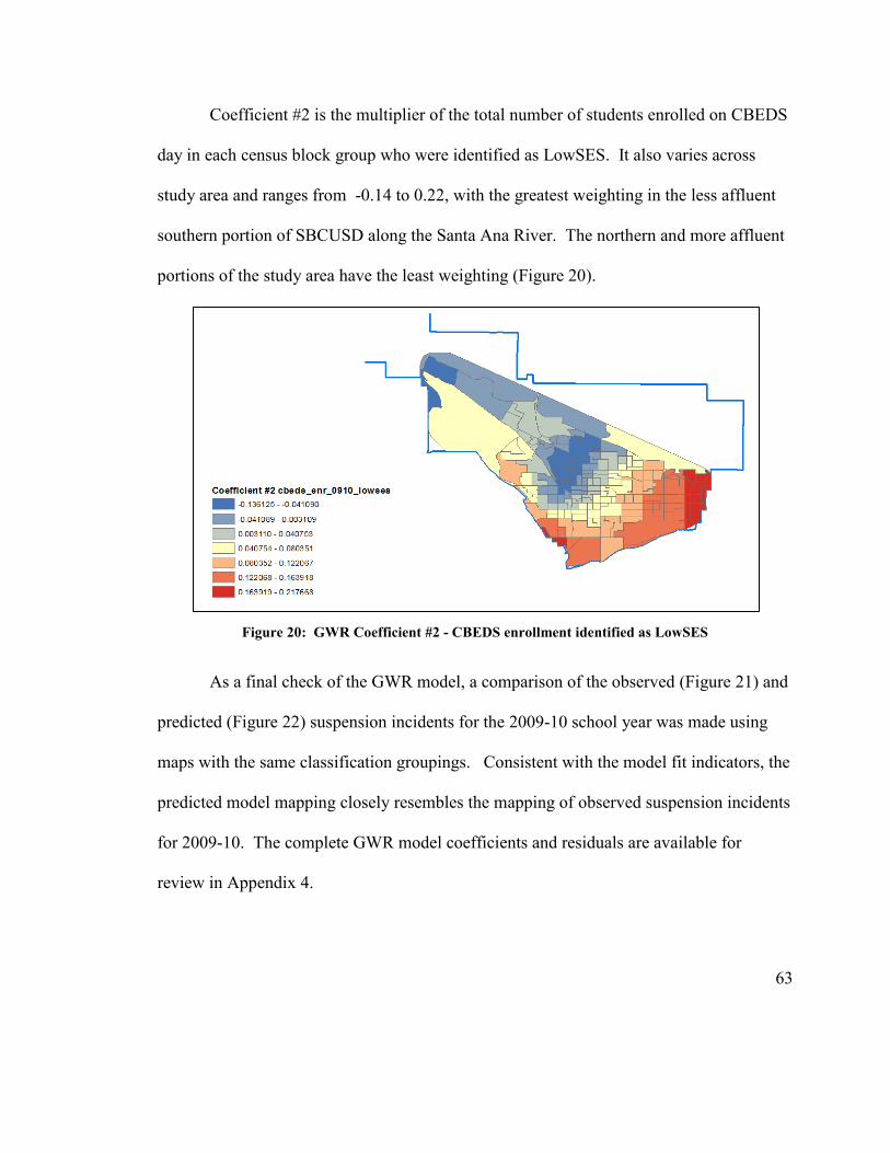
63

Coefficient #2 is the multiplier of the total number of students enrolled on CBEDS

day in each census block group who were identified as LowSES. It also varies across

study area and ranges from -0.14 to 0.22, with the greatest weighting in the less affluent

southern portion of SBCUSD along the Santa Ana River. The northern and more affluent

portions of the study area have the least weighting (Figure 20).

Figure 20: GWR Coefficient #2 - CBEDS enrollment identified as LowSES

As a final check of the GWR model, a comparison of the observed (Figure 21) and

predicted (Figure 22) suspension incidents for the 2009-10 school year was made using

maps with the same classification groupings. Consistent with the model fit indicators, the

predicted model mapping closely resembles the mapping of observed suspension incidents

for 2009-10. The complete GWR model coefficients and residuals are available for

review in Appendix 4.

64

Figure 21: 2009-10 observed suspension incidents

Figure 22: 2009-10 predicted suspension incidents, GWR Model

Predicted Susp0910_N_Incidents

65

Chapter 5

Discussion and Conclusions

The objectives of this thesis research were to (1) determine if student suspension incidents

were clustered within SBCUSD; if so, then (2) determine where incident clustering is

most intense by elementary school neighborhood; and (3) develop a regression model,

based on well-defined local factors, in order to predict overall neighborhood incident

numbers. Student datasets were processed to define a suitable study area. Multiple maps

were prepared to visualize enrollment and suspension incident patterns for all students and

significant student subgroups. Various spatial analyses were conducted and the results

were summarized in several tables. A regression model predicting overall suspension

incident numbers by census block group was prepared. Results were presented in three

sections and this same sequence is used below to discuss the wider significance of this

work.

5.1 Patterns in Student Enrollment

Investigation into patterns in student enrollment by residence within the study area

confirmed the reported high poverty rate that exists throughout SBCUSD. Only four of

the 44 elementary school neighborhoods defined in this study had less than sixty percent

of students identified as having low socioeconomic (LowSES) status. The overall district

average showed that more than 80 percent of students included in the study were

identified as LowSES. This is a significant factor that sets SBCUSD apart from many

other school districts in California and likely asserts considerable influence upon the

66

environment that leads to out-of-school student suspensions. It would be interesting to

compare the results of a similarly focused suspension study from a school district with a

low poverty rate.

In addition to poverty, enrollment patterns reported in the study area were

primarily defined in terms of race and ethnicity. Geographic distribution of enrollment by

residence among African American students (17 percent of the overall student population)

and Hispanic students (nearly 70 percent of the overall student population) in SBCUSD

covered similar areas. No elementary school neighborhood had an African American

student population of more than 30 percent, while several neighborhoods had Hispanic

student populations of nearly 90 percent of the total enrollment. White students (10

percent of the overall student population) within the district have a geographic distribution

with a center that lies more northward and runs along the foothills of the city. Many

elementary school neighborhoods along the foothills have White student populations that

are more than 20 percent of the enrollment total. In order to better understand the

distribution of ethnicities in the district and possibly help interpret the suspension

grouping patterns observed in Section 4.2.3, additional work should be done to quantify

clustering of significant subgroups at a local level.

Finally, many but not all of the neighborhoods with high enrollment densities were

also identified as neighborhoods having higher than average rates of suspension incidents

clustering. Understanding how elementary school neighborhoods like Emmerton-

Rodriguez and Mt. Vernon with similar student enrollment densities (approximately 2,000

67

students per square mile) might differ in ways that influence the numbers of students

suspended would be an important for follow-up. Having constructed the study area using

the 2010 Census Block Groups, it should be possible to compare and contrast these

neighborhoods using the published US Census Bureau 5-year American Community

Survey results (US Census Bureau 2011a).

5.2 Analysis of Student Suspensions

Strong evidence exists indicating that suspension incident clustering does occur within the

elementary school neighborhoods of SBCUSD. As measured by Moran’s Global I,

distance bands of suspension incidents for all students had Z-scores greater than 2.58

indicating significant positive spatial autocorrelation of suspension incidents (p<0.01),

thus disproving the null hypotheses of this thesis that suspension incidents for all students

are evenly distributed geographically over neighborhoods throughout the entire school

district. Significant results were also observed for the study’s subgroups by race and

ethnicity, low socioeconomic status, and suspension incident type. It would be interesting

to compare suspensions within SBCUSD to a school district with a more equal

heterogeneous race and ethnic mixture of students.

At the local level, analysis of suspension incidents for all students and subgroups

within the study area showed hotspot patterns within the district by census block group

and elementary school neighborhoods. A suspension incident clustering profile was

developed and, using a choropleth map, suspension incident hot-spot patterns were

visualized across the district by elementary school neighborhood. In particular, those

68

neighborhoods identified as group 1 in the southeast portion of SBCUSD showed the

greatest percent of suspension incident clustering for all students among all elementary

school neighborhoods, a near equal balance of suspension incident clustering between the

African American and Hispanic subgroups, and have higher levels of incident clustering

for the Low SES, Defiance and Violence subgroups. Additional studies need to be

conducted to see if these trends in suspension incident patterns hold true over multiple

years within the district. If so, understanding how these elementary school neighborhoods

differ from the others in the study is, again, an important issue for follow-up.

5.3 Modeling Suspension Incident Rates Using Regression Analysis

Regression models were developed that demonstrate, in the case of SBCUSD, that the

strongest predictor of the total number of year-end (June) suspension incidents within a

census block group is the number of days previously suspended by students residing in the

census block group during the October enrollment census with adjustment for the number

of students living in poverty. The final GWR model developed had an overall adjusted R2

value greater than 0.90 indicating that it accounted for over 90 percent of the variance in

the model. Additional studies need to be performed to determine if this model is accurate

over multiple years. If so, it could be possible to measure the effects of a suspension

intervention program on the reduction in the number of suspension incidents by using a

counter factual analysis. In such an analysis, after accounting for all other explanatory

factors, the differences between the predicted model and actual suspension incident

numbers could be attributed to the effects of the intervention program.

69

5.4 Final Comments

Additional research needs to be conducted to verify that the patterns noted within this

thesis hold steady before any recommendation can be made to act upon the results. If

such patterns are found to hold steady between years, discipline issues within SBCUSD

may in part be influenced by local neighborhood factors. This becomes an opportunity for

the school district to act at a local level and identify strategies to reduce suspensions and

improve student outcomes.

70

References

Arcia, E. 2007. Variability in schools’ suspension rates of Black students. The Journal of Negro

Education 76(4): 597–608.

Bowditch, C. 1993. Getting rid of troublemakers: High school disciplinary procedures and the

production of dropouts. Social Problems 40(4): 493-509.

Brodbelt, S. 1978. The epidemic of school violence. The Clearing House 51(8): 383-388.

Buckley, A. 2008. Minimum Bounding Rectangle (MBR). Encyclopedia of Geographic

Information Science, ed. Kemp, K. Thousand Oaks, CA, Sage Publications, Inc., 286.

California Supreme Court. 1975. National Assn. for Advancement of Colored People v. San

Bernardino City Unified School District. 17 Cal. 3d 311. Retrieved from

http://caselaw.lp.findlaw.com/scripts/getcase.pl?court=us&vol=419&invol=565

Cantillon, D., Davidson, W., and Schweitzer, J. 2003. Measuring community social organization:

Sense of community as a mediator in social disorganization theory. Journal of Criminal

Justice 31(4): 321–339. doi:10.1016/S0047-2352(03)00026-6.

CDE. 2009. Zero tolerance. Counseling and Student Support Office, California Department of

Education. Sacramento, California.

CDE. 2011. Data Quest Website. Data and Statistics Office, California Department of Education.

Sacramento, California. Retreived from http://dq.cde.ca.gov/dataquest/.

Crowder, K. and South, S. 2003. Neighborhood distress and school dropout: The variable

significance of community context. Social Science Research, 32(4): 659–698.

doi:10.1016/S0049-089X(03)00035-8.

DataEast. 2011. XTools Pro - Extension for ArcGIS. Novosibirsk, Russia: DataEast LLC.

Retrieved from http://www.xtoolspro.com/tools.asp#d4

Drakeford, W. 2006. Racial disproportionality in school disiplinary practices (Briefing Report).

National Center for Culturally Responsive Educational Systems (NCCRES).1-16.

Retrieved from http://www.nccrest.org/Briefs/School_Discipline_Brief.pdf

Esri. 2011a. ArcGIS Desktop software version 10.0. Esri (Environmental Systems Resource

Institute), Redlands, California.

Ennett, S., Flewelling, R., Lindrooth, R., and Norton, E. 1997. School and neighborhood

characteristics associated with school rates of alcohol, cigarette, and marijuana use.

Journal of Health and Social Behavior 38(1): 55–71.

http://caselaw.lp.findlaw.com/scripts/getcase.pl?court=us&vol=419&invol=565

http://dq.cde.ca.gov/dataquest/

http://www.xtoolspro.com/tools.asp#d4

71

Esri. 2011b. ArcGIS 10.0 help file – NAD 1983/NSRS 2007. Esri, Redlands, California.

Retreived from http://help.arcgis.com/en/arcgisdesktop/10.0/help/index.html#

//003r00000009000000.htm.

Feinstein , D. 2010. Details on the Gun Free Schools Act. Webpage of US Senator Dianne

Feinstein -. Retrieved http://feinstein.senate.gov/gun_free_schools.html.

Gregory, A., Skiba, R., and Noguera, P. 2010. The achievement gap and the discipline gap: Two

sides of the same coin? Educational Researcher 39(1): 59-68.

doi:10.3102/0013189X09357621.

Guest, A. and Lee, B. A. 1984. How urbanites define their neighborhoods. Population and

Environment 7(1): 32-56.

Jordan, J. and Anil, B. 2009. Race, gender, school discipline, and human capital effects. Journal

of Agricultural and Applied Economics 41(2): 419-429.

Krezmien, M., Leone, P., and Achilles, G. 2006. Suspension, race, and disability: Analysis of

statewide practices and reporting. Journal of Emotional and Behavioral Disorders 14(4):

217-226.

Kubrin, C. and Weitzer, R. 2003. New directions in Social Disorganization Theory. Journal of

Research in Crime and Delinquency 40(4): 374–402. doi:10.1177/0022427803256238.

Laub, J. and Lauritsen, J. 1998. The interdependence of school violence with neighborhood and

family conditions. In Violence in American schools Elliott, D., Hamburg, B. and Williams,

K. eds, 127 – 155. New York: Cambridge University Press.

Leventhal, T. and Brooks-Gunn, J. 2000. The neighborhoods they live in: The effects of

neighborhood residence on child and adolescent outcomes. Psychological Bulletin 126(2):

309–337. doi:10.1037//0033-2909.126.2.309.

Martin, R. C. 2001. ABA Zero Tolerance Policy. ABA Juvenile Justice Policies. Retrieved

November 3, 2010, from http://www.abanet.org/crimjust/juvjus/zerotolreport.html

Martinez, S. 2009. A system gone berserk: How are zero-tolerance policies really affecting

schools? Preventing School Failure 53(3): 153-158.

Mendez, L. and Knoff, H. 2003. Who gets suspended from school and why: A demographic

analysis of schools and disciplinary infractions in a large school district. Education and

Treatment of Children 26(1): 30-51.

Mitchell, A. 2009. The ESRI Guide to GIS Analysis volume 2: Spatial Measurements and

Statistics. ESRI Press, Redlands, California. 21-225.

http://www.abanet.org/crimjust/juvjus/zerotolreport.html

72

Peeples, F. and Loeber, R. 1994. Do individual factors and neighborhood context explain ethnic

differences in juvenile delinquency? Journal of Quantitative Criminology 10(2): 141–157.

doi:10.1007/BF02221156.

Planty, M., Hussar, W., Snyder, T., Kena, G., KewalRamani, A., Kemp, J., Bianco, K., and

Dinkes, R. 2009. Indicator 28: Student suspensions and expulsions. The Condition of

Education 2009 (NCES 2009-081). National Center for Education Statistics, Institute of

Education Sciences, U.S. Department of Education. Washington, D.C.

SAS Institute, Inc. 2012a. JMP version 9. SAS Institute Inc., Cary, North Carolina.

SAS Institute. 2012b. Hierarchical Clustering. JMP version 9. SAS Institute Inc., Cary, North

Carolina. Retrieved from http://www.jmp.com/support/help/Hierarchical_Clustering.shtml

SBCUSD Facilities Office. 2009. SBCUSD Base Map. San Bernardino City Unified School

District, San Bernardino, California.

SBCUSD Research Office. 2010. End-of-year summary reports for suspensions, enrollment, and

mobility. San Bernardino City Unified School District, San Bernardino, California.

Skiba, R. 2000a. Zero tolerance, zero evident: An analysis of school disciplinary practice (Policy

Research Report No. SRS2). Indiana Education Policy Center: Indiana University.

Retrieved from http://scholar.google.com.libproxy.usc.edu/scholar?hl=en&

lr=&q=zero%20tolerance%2C%20zero%20evidence%20skiba

Skiba, R. 2000b. The color of discipline. Policy Research Report, Indiana Education Policy

Center. Retrieved from http://www.indiana.edu/~safeschl/cod.pdf

Skiba, R. and Peterson, R. 1999. The dark side of zero tolerence: Can punishment lead to safe

schools? Phi Delta Kappan 80(5): 372-376.

Summers, A. 1979. Angels in purgatory: Los Angeles awaits two decisions on mandatory busing

for desegregation. The Phi Delta Kappan 60(10): 718–723.

Taras, H. 2003. AAP policy statement on out-of-school suspension and expulsion (Renewed

2008). Pediatrics 112(5): 1206-1209.

Tatalovich, Z., Wilson, J., Milam, J., Jerrett, M., and McConnell, R. 2006. Competing definitions

of contextual environments. International Journal of Health Geographics 5(1): 55.

doi:10.1186/1476-072X-5-55.

Tobin, T. and Sugai, G. 1999. Using sixth-grade school records to predict school violence,

chronic discipline problems, and high school outcomes. Journal of Emotional and

Behavioral Disorders 7(1): 40-53.

http://scholar.google.com.libproxy.usc.edu/scholar?hl=en&%20lr=&q=zero%20tolerance%2C%20zero%20evidence%20skiba

http://scholar.google.com.libproxy.usc.edu/scholar?hl=en&%20lr=&q=zero%20tolerance%2C%20zero%20evidence%20skiba

http://www.indiana.edu/~safeschl/cod.pdf

73

US Census Bureau. 2010. San Bernardino County Demographic Block Groups shapefile

(Tl_2010_0607_bg10). 2010 Tiger Line Shapefiles. Retreived from

http://www.census.gov/cgi-bin/geo/shapefiles2010/main

US Census Bureau. 2011a. Comparing ACS Data. American Community Survey. Retreived from

http://www.census.gov/acs/www/guidance_for_data_users/comparing_data/

US Census Bureau. 2011b. San Bernardino California – Poverty Table. 2010 American

Community Survey 1-Year Results. Retreived from

http://factfinder2.census.gov/faces/nav/jsf/pages/searchresults.xhtml?refresh=t

US Department of Education . 2010. Duncan speaks at Dr. King’s church on 81st birthday of the

legendary civil rights leader. Press Releases: January 15, 2010. Retrieved June 3, 2010,

from http://www2.ed.gov/news/pressreleases/2010/01/01152010.html

US Supreme Court. 1975. Goss v. Lopez. 419 USC 565 1975. Retreived from

http://www.law.cornell.edu/supct/html/historics/USSC_CR_0419_0565_ZS.html

Williams, T., Davis, L., Saunders, J., and Williams, J. 2002. Friends, family, and neighborhood:

Understanding academic outcomes of African American youth. Urban Education 37(3):

408 –431. doi:10.1177/00485902037003006.

Wu, S., Pink, W., Crain, R., and Moles, O. 1982. Student suspension: A critical reappraisal. The

Urban Review 14(4): 245-303.

http://www.census.gov/cgi-bin/geo/shapefiles2010/main

http://factfinder2.census.gov/faces/nav/jsf/pages/searchresults.xhtml?refresh=t

http://www2.ed.gov/news/pressreleases/2010/01/01152010.html

http://www.law.cornell.edu/supct/html/historics/USSC_CR_0419_0565_ZS.html

74

Appendix 1

SBCUSD Notice of Suspension

Appendix 1

75

Appendix 2

SBCUSD Suspension Incident Rank Reporting Plan

76

Appendix 3

OLS Summary of Results

77

Appendix 4

GWR Model by Census Block Group

Object

ID

2009-10

Suspension

Incidents

2009-10

CBEDS Enr N

Days Susp

2008-09

2009-10

CBEDS Enr N

Low SES LocalR2 Predicted Intercept

Coefficient

#1

Coefficient

#2 Residual

1 330 192 713 0.920764 329.644201 -16.248372 1.364848 0.117589 0.355798

2 37 34 62 0.915196 51.566939 2.234735 1.17202 0.152959 -14.566939

3 85 62 179 0.92675 91.388068 -18.507404 1.561508 0.073083 -6.388068

4 177 113 651 0.927351 205.732257 -21.675898 1.567811 0.077181 -28.732257

5 178 92 451 0.920374 161.776293 -13.6301 1.418986 0.099466 16.223706

6 1 0 5 0.918514 -10.987524 -11.747625 1.201812 0.15202 11.987524

7 50 25 182 0.925798 34.300365 -16.425329 1.606513 0.058037 15.699634

8 241 163 544 0.919477 272.164063 -9.109539 1.458001 0.080182 -31.164063

9 123 90 233 0.923575 139.972093 -13.334111 1.502888 0.077451 -16.972093

10 64 46 343 0.925057 76.103711 -19.369022 1.616076 0.061612 -12.103711

11 105 57 263 0.919716 95.703191 -3.12962 1.557467 0.03824 9.296808

12 131 69 221 0.912129 112.51768 -1.805542 1.419416 0.074133 18.482319

13 237 165 522 0.919374 270.924723 -14.219998 1.373106 0.112226 -33.924723

14 37 18 120 0.868805 22.448611 -3.657733 1.826983 -0.056494 14.551388

15 83 41 207 0.789048 58.053285 -22.335332 1.03417 0.183515 24.946714

16 46 30 85 0.923114 45.849428 -5.192742 1.659569 0.014765 0.150571

17 44 40 174 0.764678 61.174129 9.238996 1.311954 -0.00312 -17.174129

18 161 118 333 0.814723 163.342451 8.376217 1.3045 0.003108 -2.342451

19 123 109 420 0.814609 146.985029 16.712029 1.067818 0.033049 -23.985029

20 132 86 275 0.829114 118.682501 14.326584 1.11584 0.030522 13.317498

21 170 103 257 0.925232 164.343154 -12.32285 1.569908 0.058231 5.656845

22 14 10 54 0.90545 21.801383 8.449151 1.035274 0.055545 -7.801383

23 104 72 197 0.824248 99.791731 14.247418 1.132553 0.020307 4.208268

24 86 55 159 0.909712 88.315545 -6.011269 1.775071 -0.020767 -2.315545

25 89 71 226 0.920523 115.013265 -5.342255 1.534241 0.05055 -26.013265

26 18 9 47 0.911752 16.715309 1.024138 1.47164 0.052051 1.28469

27 105 41 249 0.909826 75.893474 0.293865 1.413508 0.070866 29.106525

28 119 60 182 0.915167 97.520569 -1.545334 1.487026 0.054089 21.47943

29 127 75 300 0.910948 120.486509 -16.99814 1.679451 0.038419 6.51349

30 38 42 141 0.904295 52.837543 -24.914511 1.58149 0.08035 -14.837543

31 107 79 336 0.91585 127.168471 -24.641639 1.596634 0.076416 -20.168471

32 115 62 295 0.91063 97.053654 -23.366038 1.62247 0.067208 17.946345

33 51 32 137 0.867249 37.294658 -22.76526 1.569105 0.071887 13.705341

34 245 140 407 0.911744 232.820772 -2.773452 1.805112 -0.042067 12.179227

35 99 46 169 0.910932 73.253736 -1.327522 1.818182 -0.05358 25.746263

36 62 45 174 0.800611 68.967549 13.067427 1.142765 0.025722 -6.967549

37 100 75 193 0.871811 100.023438 9.460461 1.226979 -0.007567 -0.023438

38 66 43 286 0.692045 65.763047 -4.865518 1.299524 0.05157 0.236952

39 119 112 350 0.867157 179.025468 -21.060289 1.607254 0.057352 -60.025468

40 146 78 208 0.88249 118.339578 -20.13802 1.648307 0.047642 27.660421

41 280 153 548 0.858281 252.334604 -14.115355 1.70334 0.010654 27.665395

42 184 98 329 0.897013 159.130395 -17.44179 1.688005 0.033883 24.869604

43 184 93 409 0.894797 153.427152 -18.860683 1.673333 0.040752 30.572847

44 455 250 715 0.915721 430.930887 -19.207584 1.656896 0.050229 24.069112

45 64 29 129 0.84961 40.510948 -6.257892 1.795498 -0.041089 23.489051

46 158 134 325 0.866512 219.575963 -12.91402 1.729269 0.002362 -61.575963

47 236 121 335 0.871154 198.17854 -11.551002 1.749837 -0.005972 37.821459

48 136 62 251 0.903208 97.601438 -12.451315 1.727272 0.0118 38.398561

49 160 65 248 0.870579 101.263546 -8.344093 1.787921 -0.026642 58.736453

50 131 105 428 0.694494 152.538366 -1.467381 1.380559 0.021137 -21.538366

51 103 87 323 0.701329 125.984974 2.375895 1.470372 -0.013353 -22.984974

52 151 101 463 0.641087 137.346526 12.10589 1.246596 -0.001437 13.653473

53 104 93 363 0.643524 125.484372 14.827356 1.128171 0.015804 -21.484372

54 147 106 319 0.850974 143.267407 12.222473 1.180318 0.018593 3.732592

55 56 43 240 0.691344 63.75412 -7.68695 1.225039 0.078184 -7.75412

56 111 53 137 0.888737 81.470657 -11.002696 1.756654 -0.004593 29.529342

57 93 76 322 0.915444 123.954859 -13.361927 1.690968 0.027338 -30.954859

58 18 15 100 0.896915 16.702555 -8.269753 1.777516 -0.016904 1.297444

59 24 19 110 0.89663 22.918965 -9.65673 1.763591 -0.008477 1.081034

Observed GWR Model

78

Appendix 4 (Cont’d.)

Object ID

2009-10

Suspension

Incidents

2009-10

CBEDS Enr N

Days Susp

2008-09

2009-10

CBEDS Enr N


Coefficient

#1

Coefficient

#2 Residual

60 42 37 124 0.919542 54.923592 -10.008217 1.692575 0.0186 -12.923592

61 108 56 220 0.911324 89.063118 -4.455379 1.787582 -0.029936 18.936881

62 81 39 233 0.921523 60.216112 -12.459139 1.66524 0.033179 20.783887

63 104 63 189 0.884757 101.271805 -3.308038 1.821304 -0.053769 2.728194

64 47 26 117 0.893358 36.78806 -6.334282 1.801357 -0.031734 10.211939

65 19 18 106 0.910438 22.928229 -7.784417 1.753838 -0.008079 -3.928229

66 70 32 274 0.838558 57.551185 -23.809387 1.235672 0.152624 12.448814

67 68 37 356 0.772433 54.399663 -9.849764 1.547269 0.019664 13.600336

68 61 57 256 0.806664 84.142907 -7.160632 1.699205 -0.021684 -23.142907

69 43 38 219 0.794156 52.650257 -1.578573 1.738183 -0.053982 -9.650257

70 46 21 153 0.783438 28.436787 2.711915 1.698951 -0.065052 17.563212

71 59 30 231 0.782117 38.359659 2.016717 1.71649 -0.065592 20.64034

72 27 33 97 0.92083 49.556212 -7.428251 1.700471 0.008957 -22.556212

73 0 0 0 0.841692 -21.91135 -21.91135 1.010619 0.198305 21.91135

74 0 0 0 0.726038 -19.239688 -19.239688 0.796357 0.213501 19.239688

75 0 0 0 0.735877 -19.819198 -19.819198 0.858597 0.203859 19.819198

76 15 16 53 0.866644 27.907383 7.660412 1.312247 -0.014131 -12.907383

77 0 0 0 0.999299 6.736258 6.736258 1.596282 -0.136125 -6.736258

78 14 6 14 0.903434 14.78961 5.552325 1.371456 0.072039 -0.78961

79 64 50 157 0.879969 77.029712 -0.565428 1.667192 -0.036716 -13.029712

80 23 16 70 0.999422 22.937635 6.884021 1.586501 -0.133291 0.062364

81 180 105 767 0.699951 164.610957 26.4505 0.669072 0.088536 15.389042

82 206 119 370 0.908186 193.090818 -1.662829 1.25705 0.122066 12.909181

83 135 98 383 0.923192 161.442625 -18.950161 1.37106 0.120179 -26.442625

84 167 112 400 0.925015 185.234929 -16.744472 1.504554 0.083673 -18.234929

85 0 0 0 0.917754 -6.876316 -6.876316 1.131622 0.16308 6.876316

86 106 60 300 0.576549 89.175453 20.360963 0.828941 0.063593 16.824546

87 120 67 218 0.823364 95.568532 12.11046 1.171336 0.022837 24.431467

88 0 0 0 0.947422 -5.278829 -5.278829 1.090597 0.217668 5.278829

89 0 0 1 0.94201 -3.895823 -4.107998 1.088279 0.212174 3.895823

90 99 55 328 0.914522 101.840294 -8.799112 1.328493 0.114549 -2.840294

91 29 22 98 0.924794 29.407589 -10.308972 1.586645 0.049085 -0.407589

92 124 97 269 0.924066 153.342305 -20.873244 1.619463 0.063671 -29.342305

93 53 36 106 0.923945 53.180283 -8.617291 1.577614 0.047202 -0.180283

94 258 131 659 0.774822 228.548369 -21.118081 1.181592 0.143972 29.45163

95 19 17 38 0.929537 25.243873 -0.989613 1.137841 0.18132 -6.243873

96 65 35 210 0.906627 68.463337 -0.057959 1.275745 0.113667 -3.463337

97 75 31 155 0.906117 60.310174 2.720102 1.223259 0.126896 14.689825

98 0 0 0 0.932314 -1.173436 -1.173436 1.084607 0.199287 1.173436

99 51 33 174 0.920219 69.326406 2.959312 1.101377 0.172538 -18.326406

100 151 95 312 0.913726 158.036057 2.787508 1.123693 0.155441 -7.036057

101 157 111 732 0.774513 162.813016 18.376785 0.970732 0.050116 -5.813016

102 178 121 586 0.788701 166.194719 18.821469 0.971081 0.050976 11.80528

103 160 140 598 0.692771 189.78403 9.499575 1.397621 -0.025723 -29.78403

104 141 83 325 0.910095 143.743136 -0.429995 1.18571 0.140797 -2.743136

105 168 91 430 0.912339 172.126444 3.015792 1.139252 0.152182 -4.126444

106 292 187 523 0.908875 295.659295 0.035908 1.198919 0.136568 -3.659295

107 4 1 12 0.940449 -0.029612 -3.583946 1.106897 0.203953 4.029612

108 97 48 162 0.905833 80.260263 1.008224 1.303733 0.102918 16.739736

109 76 36 200 0.925135 48.036127 -24.970372 1.56644 0.083073 27.963872

110 105 53 217 0.712559 78.065807 5.045516 1.534492 -0.038284 26.934192

111 74 80 286 0.769618 120.560211 -0.976019 1.676072 -0.043879 -46.560211

112 81 93 332 0.584527 120.978958 8.820912 0.885561 0.089761 -39.978958

113 8 2 18 0.936931 3.145942 -2.699236 1.095178 0.203045 4.854057

114 86 29 194 0.923067 69.031561 2.339229 1.086146 0.181412 16.968438

115 243 111 721 0.911395 228.381856 -4.709305 1.234725 0.133199 14.618143

116 165 110 284 0.90857 170.709159 -1.202236 1.226519 0.130261 -5.709159

117 206 98 449 0.911207 183.153654 3.074574 1.155089 0.148953 22.846345

118 18 16 80 0.928296 32.221296 -0.419824 1.119638 0.184086 -14.221296

GWR ModelObserved

79

Appendix 4 (Cont’d.)

Object ID

2009-10

Suspension

Incidents

2009-10

CBEDS Enr N

Days Susp

2008-09

2009-10

CBEDS Enr N


Coefficient

#1

Coefficient

#2 Residual

119 118 70 243 0.85679 106.929028 -15.868828 1.675368 0.022724 11.070971

120 181 119 514 0.888111 183.518359 -1.965652 1.798162 -0.055442 -2.518359

121 86 56 204 0.863811 85.699235 -0.839563 1.745245 -0.054877 0.300764

122 68 52 159 0.867346 76.228945 5.823309 1.338198 0.005152 -8.228945

123 91 47 181 0.899345 73.233445 -1.658002 1.804799 -0.054884 17.766554

124 84 61 191 0.81286 94.350309 1.362073 1.728417 -0.065158 -10.350309

125 0 0 0 0.837506 -22.081452 -22.081452 1.01307 0.197389 22.081452

126 18 16 48 0.925981 26.618169 -0.050564 1.135133 0.17722 -8.618169

127 73 31 209 0.925997 73.07479 0.551124 1.110648 0.182265 -0.07479

128 35 13 103 0.903958 30.703557 3.620336 1.302618 0.098535 4.296442

129 0 0 0 0.686483 -15.401789 -15.401789 0.695833 0.21711 15.401789

130 0 0 3 0.9115 3.32837 2.892035 1.180595 0.145445 -3.32837

131 237 122 422 0.913387 208.757118 2.775869 1.162022 0.152167 28.242881

132 249 136 406 0.918202 222.364417 -5.994755 1.473933 0.068729 26.635582

133 75 41 171 0.923738 58.616134 -17.50507 1.632514 0.053731 16.383865

134 124 94 268 0.595859 118.492884 18.890967 0.925061 0.047186 5.507115

135 123 90 532 0.703495 127.524636 15.251156 1.079206 0.028467 -4.524636

136 151 161 603 0.622022 213.423807 9.320987 1.171533 0.025681 -62.423807

137 46 31 139 0.859139 44.856441 -3.809538 1.824825 -0.05686 1.143558

138 59 56 268 0.840046 82.496583 -3.862758 1.807658 -0.055483 -23.496583

139 99 49 218 0.886005 69.889586 -25.348719 1.510996 0.097245 29.110413

140 52 30 156 0.888188 37.981945 -23.5153 1.330118 0.138421 14.018054

141 46 21 134 0.905027 45.025585 3.034158 1.250168 0.117446 0.974414

142 62 18 108 0.913958 39.702195 2.434625 1.188202 0.147036 22.297804

143 132 78 231 0.913466 128.420366 2.927932 1.154329 0.153483 3.579633

144 124 44 265 0.916713 95.892359 3.741471 1.107107 0.163917 28.10764

145 35 23 97 0.916459 44.839245 3.256878 1.122309 0.162569 -9.839245

146 215 101 402 0.916655 182.383158 2.79569 1.133054 0.162062 32.616841

147 58 32 144 0.836439 49.019303 5.22223 1.407965 -0.008734 8.980696

148 79 61 155 0.831378 88.266354 8.148599 1.299904 0.005313 -9.266354

149 0 0 0 0.684979 -14.943197 -14.943197 0.754353 0.203467 14.943197

150 0 0 0 0.57363 23.753636 23.753636 0.69294 0.083433 -23.753636

151 96 70 394 0.764867 102.191479 -4.571703 1.611491 -0.015333 -6.191479

152 93 49 239 0.815031 70.908492 -12.160829 1.641753 0.010976 22.091507

153 195 110 369 0.911141 182.216429 -15.446636 1.689427 0.032048 12.78357

154 85 63 312 0.849074 96.798496 -17.4875 1.634108 0.036337 -11.798496

155 253 131 481 0.915648 221.914873 -21.499994 1.640834 0.059179 31.085126

156 144 88 375 0.902675 144.325551 -21.20556 1.64881 0.054495 -0.325551

157 132 85 357 0.929354 137.471002 -24.789805 1.497583 0.097944 -5.471002

158 130 79 433 0.911187 155.456453 0.288308 1.163743 0.146033 -25.456453

159 107 98 471 0.631146 132.098949 21.661666 0.8203 0.063795 -25.098949

160 147 109 448 0.686508 160.862704 -12.838362 0.983776 0.148369 -13.862704

161 21 4 37 0.922219 4.958438 -1.573382 1.696481 -0.006867 16.041561

162 121 79 328 0.87441 119.215441 -0.729843 1.709653 -0.046089 1.784558

163 145 108 370 0.848398 159.314766 2.03653 1.544723 -0.025815 -14.314766

164 124 93 277 0.83169 139.309693 2.295204 1.579796 -0.035764 -15.309693

165 117 83 441 0.803871 133.560512 -17.006495 1.510899 0.057057 -16.560512

166 152 64 443 0.798958 113.372668 -21.211474 1.351241 0.108588 38.627331

167 103 56 366 0.755993 87.772889 -12.646747 1.423283 0.0566 15.22711

168 69 58 268 0.928399 87.547069 -25.748607 1.481398 0.102143 -18.547069

169 245 148 513 0.914631 246.981897 -5.97673 1.396932 0.090083 -1.981897

170 86 86 342 0.910916 146.055831 -2.523592 1.376445 0.088318 -60.055831

171 190 104 382 0.913878 173.570054 -7.183994 1.353598 0.104659 16.429945

172 230 144 259 0.907988 212.228971 -1.61535 1.275431 0.116533 17.771028

173 198 85 536 0.913026 173.675951 -4.920708 1.198979 0.143066 24.324048

174 137 79 482 0.928072 139.606955 -23.555515 1.54713 0.084935 -2.606955

175 0 0 1 0.932747 -26.588505 -26.731982 1.318292 0.143477 26.588505

176 132 100 325 0.907066 165.60365 1.849279 1.208427 0.132035 -33.60365

177 63 47 156 0.811197 71.532861 2.548283 1.630931 -0.049161 -8.532861

GWR ModelObserved

OUT-OF-SCHOOL SUSPENSIONS BY HOME NEIGHBORHOOD: by …

Documents

Transcript of OUT-OF-SCHOOL SUSPENSIONS BY HOME NEIGHBORHOOD: by …