OUT-OF-SAMPLE PERFORMANCE OF MEAN-VARIANCE STRATEGIES:IS ACTIVE PORTFOLIO

MANAGEMENT WORTH THE EFFORT IN EUROPE?

Francisco J. Navarro Sánchez

Trabajo de investigación 013/015

Master en Banca y Finanzas Cuantitativas

Tutores: Dr. Martín Lozano

Universidad Complutense de Madrid

Universidad del País Vasco

Universidad de Valencia

Universidad de Castilla-La Mancha

www.finanzascuantitativas.com

Out-of-Sample Performance of Mean-Variance Strategies:

Is Active Portfolio Management Worth the Effort in Europe?

Francisco J. Navarro Sánchez

Tutor: Martín Lozano

ABSTRACT

In the present work we evaluate the performance out-of-sample of 14 mean-variance

strategies. We use two approaches, one is the classical where we obtain only one

result for each measure based on the whole data period available, and other when

we define different sub-periods that only change by two dates with the following

allowing to evaluate the evolution over time of strategies’ performance. We try to

determine if active portfolio management leads to a better performance that simply

allocate wealth in equal parts among all risky assets in data sets formed with

portfolios from 10 European countries. We conclude that for the classical approach

there actually some strategies that outperform naïve diversification whether we

consider or not transaction costs, proving the utility of optimization strategies. These

outperformers all consider multiple simplifications and restriction over mean-

variance framework and low turnover. When considering sub-periods, we can

observe that changes among sub-periods are important, so performance is heavily

influenced by the data, nevertheless the best performers maintain their order of

preference and therefore our results for the whole period are robust.

I. Introduction

Portfolio performance is one of the most attractive topics in finance because of its applicability, as

it is devoted to construct actual recommendations to short-term investors. Since the seminal

paper from Markowitz (1952), mean-variance optimization has been the most important

framework in portfolio management, but although its optimal performance when moments of

risky assets are known, this performance is not achieved when these moments have to be

estimated, leading to portfolios weights recommended by this strategy that achieve bad out-of-

sample results, so its theoretical usefulness is reduced by its empirical performance. This has

generated a vast amount of literature that try to deal with these estimation errors, resulting in

multiple strategies that try to improve out-of-sample mean-variance performance.

DeMiguel, Garlappi and Uppal (2009) evaluate 14 different strategies from 7 data sets from the

market concluding that none of them outperforms a naïve strategy which relies in allocate total

wealth in equal parts between all the risky assets, in all the measures studied, Sharpe ratio,

certainty equivalent, turnover and return loss, and data sets analyzed, therefore casting doubt on

usefulness of active portfolio management. We follow a similar approach; therefore we also

compare a set of 14 strategies using the same measures and methodology to determine their

performance.

Hence, the main objective of this work is, as in DeMiguel, Garlappi and Uppal (2009), to compare

out-of-sample performance of mean-variance strategy and their extensions, which on most cases

try to improve their performance by making assumptions and simplifications that although do not

hold for the data and thus suppose specification errors, reduce the number of parameters

estimated and so their errors. This comparison will determine first if active management portfolio

beats naïve diversification and therefore is useful for an investor interested in the European

markets, and second a strategies’ order of performance that permits making recommendations to

an investor interested in the markets analyze, obviously an investor would be interested in

maximize its benefits so we account for that with a measure of risk-adjusted performance, Sharpe

ratio, a measure of utility maximization, certainty equivalent, and a more realistic measure

because takes into consideration transaction costs, return loss.

Our contributions to this extent literature are: (1) to add more recent proposed strategies, (2) use

of European capital markets and (3) evolution of performance among sub-periods. We consider

recent strategies as the ones of Kirby and Ostdiek (2012), which try to introduce naïve

diversification benefits in active portfolio management by determine portfolio weights by changes

in variance but not in covariances, and Tu and Zhou (2011) which calculates the optimal

combination rule between different asset allocation strategies and naïve diversification, strategies

that have been little explored. As opposed to other empirical works which have focus mainly in the

US market, we contribute to the growing but still limited literature regarding the European capital

market, more precisely we consider ten different countries that include the most important

markets of the area. And apart from the standard methodology where portfolio performance is

reduced to a single value for the whole data available, we also present this performance as a

series of results by using rolling sub-periods of a length of 300 months starting from the beginning

of our data and then we move the initial and final date one month ahead, with this approach we

can determine if conclusions regarding strategies comparisons are robust in the sense that they

are evaluated not only in one single period, and also evaluate how different are the results

achieved by changing only two data at a time, which has not been previously tested in historical

data sets.

Our main results are: (1) active management strategies can outperform naïve diversification for all

datasets, (2) performance varies greatly among sub-periods and (3) results from sub-periods are

consistent with the ones of the whole period. Contrary to that showed DeMiguel, Garlappi and

Uppal (2009) there are various strategies that outperform naïve diversification in our samples,

especially when the number of assets is small, proving that estimation errors grow as does the

number of parameters to be estimated, so there is a benefit for an European investor to

implement an active portfolio management. From all the strategies, minimum variance performs

the best in Sharpe ratio and certainty equivalent in all of our data sets, surprisingly for the less

aggressive strategy which targets a low return, but only optimizing variance-covariance matrix and

not expected returns really helps reducing estimation error. If we account for transaction cost,

adding a short selling restriction to minimum variance improves its performance due to a

reduction in turnover which compensates for the loss in Sharpe ratio and certainty equivalent

performance. The two strategies of Kirby and Ostdiek (2012) performs considerably well, beating

naïve diversification, despite the fact that both use mean-variance portfolio weights assuming

correlation between pairwise assets to be zero, which does not occur in the data, but the gains of

no estimating them outperforms the losses due to specification error. These results are similar to

what they obtained in the more similar dataset, when assets are ordered by size and book-to-

market, where also both strategies outperform naïve diversification. The others strategies that

work better than naïve diversification are combinations of naïve diversification and minimum

variance with and without short selling, but their results are not as good as the uncombined

strategies. Tu and Zhou (2011) show that combining strategies with naïve diversification improves

their results, as in their paper that is true when we combine the tangency portfolio with naïve

diversification but still is not enough to outperform this simple 1/N rule. From these results we can

conclude that this kind of combination improves a strategy performance when their individual

performance is worse than naïve diversification, but not when is better. On the contrary, the

tangency portfolio that follows Markowitz’s methodology and does not account for estimation

errors obtains the worst results of all the strategies, so estimation errors completely erodes the

benefits of an in-sample optimal strategy with also extreme turnovers due to unstable portfolio

weights.

By analyzing the results of the strategies in different sub-periods that only change by two dates,

we can observe that these changes can be enormous, so caution should be taken when reducing

all the performance of an strategy to a single number, as the data utilized affects greatly.

Nevertheless, strategies which perform better in the whole period are also the ones that

outperform the others in almost all the sub-periods so our results from the whole period are

robust, with the exception of the most recent dates, starting in sub-periods that last from 1986 to

2011. In these sub-periods even the tangency portfolio obtains greats Sharpe ratio and specially

certainty equivalent. The reason behind this is obvious, if the estimations are correct, TP is the

optimal strategy, therefore in these recent dates estimations are more near the real ones, so TP

achieve better performance, but even in this near optimal situation, the amount of changes in

portfolio weights needed to follow this strategy generates an amount of transaction costs that

eliminate the benefits of this strategy.

The rest of the dissertation is organized as follows. In section II, we enumerate a bibliographic

review of the literature on mean-variance framework and their extensions to deal with estimation

risks. Section III describes the various strategies of asset allocation we compare. In section IV, we

list the data from European countries we use to analyze strategies’ performance. Section V

provides the methodology and measures employed to evaluate strategies’ out-of-sample

performance. In section VI, we show the empirical results from these measures when we consider

only one period which covers all the data available. Section VII show these results when we

consider a set of sub-periods and provides performance’s evolution of asset allocation strategies.

And section VIII concludes.

II. Bibliographic review

The seminal paper of Markowitz (1952) introduced a methodology that have since then been known as Modern Portfolio Theory. Markowitz’ work develops the optimal rule for investors to allocate their wealth in risky assets in a one period universe, considering only the mean and variance of the portfolio returns. But as already appointed by Markowitz, this procedure is the second stage in the process of selecting a portfolio, while the first stage comprise finding the first two moments of the risky assets to form the portfolio. Because these moments are not known, they have to be estimated, the simple way by substituting them with their sample counterparts based on historical data of the risky assets. But this leads to estimation errors, and therefore a worse performance out-of-sample1, and these errors can be so massive than even mean variance optimization can be outperformed by naïve diversification which allocates total wealth in equal parts among risky assets as observed by an experiment on three assets designed by Frankfurter, Phillips and Seagle (1971).

There is an extensive literature that tries to address this issue2 applying different methodologies to improve out-of-sample performance. We briefly describe the most important approaches proposed by the literature.

First, there are a wide variety of Bayesian approaches which relying in Bayes’ rule. A Bayesian investor considers the distribution of parameters given by Bayes’ rule obtained from some data

1 Michaud (1989) show that extreme and unstable portfolio weights are inherent to mean-variance

optimizers because they tend to assign large positive (negative) weights to securities with large positive (negative) estimation errors in the risk premium and/or volatility. 2 See Brandt (2010) and Chapados (2011) for a more exhaustive description of the portfolio problems and its

solutions.

and a subjective prior distribution on parameters values. The different methodologies depend on the prior chosen and range from methodologies relying in diffuse-priors as Klein and Bawa (1976), Bawa, Brown and Klein (1979) and Brown (1979), where a diffuse-prior is a distribution of the parameter with equal probability for each possible value and therefore is a non-informative prior, while others priors based on a belief in an asset pricing model as Pastor (2000) and Pastor and Stambaugh (2000), use of an underlying economic equilibrium model combined with the investor’s views to provide the prior like in Black and Litterman (1992) or dealing with model uncertainty by averaging over plausible model specifications as Avramov (2002) and Tu and Zhou (2004).

Stein (1956) and James and Stein (1961) pioneered the idea of shrinkage estimators. They showed that sample means is an inadmissible estimator when , and find that a shrinkage estimator dominates it. It is called a shrinkage estimator because it shrinks the value of the estimator to a common value (shrinkage target), so tends to pull the most extreme coefficients to this common value. It can be interpreted as a Bayesian approach where the shrinkage target is the prior and the confidence in that prior determines how much the estimators are shrunk. This methodology has been applied to the estimation of the expected returns by Jobson, Korkie and Ratti (1979) or Jorion (1986) who shrinks it to the mean of the minimum variance strategy; also has been used to improve the estimation of the covariance matrices as Frost and Savarino (1986) which shrinks expected returns, variances and correlations towards their respective average, because the more extreme a coefficient is the more likely it has been estimated with error, or Ledoit and Wolf (2004) which shrinks the correlation matrix; and even to portfolio weights as Brandt (2010) who show how can be applied to the plug-in estimates of the optimal portfolio weights where the shrinkage target can be naïve diversification.

Goldfarb and Iyengar (2003) based on limited information of the parameters define sets of values that are consistent with this information, and then select portfolios weights that perform well for all these values, therefore the optimization problem is now to maximize the worst case scenario, that is called robust portfolio selection problems. The objective of this strategy is to reduce the sensitivity of portfolio weights to perturbations in the estimators.

Other strategies try to improve performance by imposing restrictions on the estimation of the moments of the risky assets. The most known is the minimum variance strategy which selects portfolio weights without estimating expect returns, this way reduces the number of parameters to be estimate resulting in lesser estimation errors but a cost of a loss of information, therefore their performance depends in the trade-off between these two opposite effects. MacKinlay and Pástor (2000), on the other hand, assume that given a factor-based pricing model with no observed factors, expected returns are strongly linked to covariance matrix of returns, and this leads to a simplification in which an identity matrix can be used as a covariance matrix when calculating the tangency portfolio weights.

Additionally, constraints can be imposed to portfolio weights. Frost and Savarino (1988) analyze constraints on the maximum proportion of a portfolio than can be invested in a single asset while Jagannathan and Ma (2003) also study the performance of portfolios when short-selling is not allowed. These restrictions can improve strategies’ performance if extreme values of the estimators are likely to be caused by estimation error.

Finally, strategies can be combined with others as Kan and Zhou (2007) who analytically proved that when estimation errors exists Markowitz’s two-fund rule, which implies that exists a combination of the free-risk asset and a portfolio of risky assets which is optimal for a mean

variance investor, is indeed not optimal and can be improved. They proposed combine mean variance strategy with the minimum variance portfolio because although both have estimation errors, they are not perfectly correlated and can be diversified.

Despite these improvements, DeMiguel, Garlappi and Uppal (2009) compare naïve diversification

with 14 different portfolio strategies, which apply several of the previously commented

methodologies, in 7 different empirical data sets, obtaining than none is consistently better than

the naïve rule, casting doubt upon the utility of the mean-variance framework. In contrast with

these results, Tu and Zhou (2011) combine the naïve rule with four portfolio rules obtaining better

results than the uncombined strategies and beating the naïve rule specially when sample size

increase, while Kirby and Ostdiek (2012) find flaws in DeMiguel, Garlappi and Uppal (2009) that

partly explain the good results of the naïve rule, and also propose two families of strategies that

can improve results.

III. Description of portfolio allocation strategies

In this section we describe the 14 portfolio allocation strategies from the literature on the mean-

variance framework whose out-of-sample performance we compare in order to identify which

ones outperforms the others, also performance of these strategies will allow us to determine how

estimation errors reduce or eliminate the gains from portfolio optimization in empirical data.

These strategies have been selected to show different approximations to deal with these errors.

We have limited to strategies that only consider the first two moments of asset returns, but not

other characteristics or information of the assets or the market, such as a belief in an asset pricing

model as does Pastor (2000), therefore we restrain Bayesian approach to uninformative priors.

Before beginning with the description of these strategies and how they allocate wealth among

risky assets, we briefly formulate the basic framework of mean-variance as pioneered by

Markowitz (1952). In this seminal paper, he derived the optimal rule for allocating wealth across

risky assets in a static setting when investors have a quadratic utility function where they consider

expected return a desirable thing and variance of return undesirable. Therefore if we denote to

the -dimensional vector of portfolio weights invested in the risky assets in date , investors

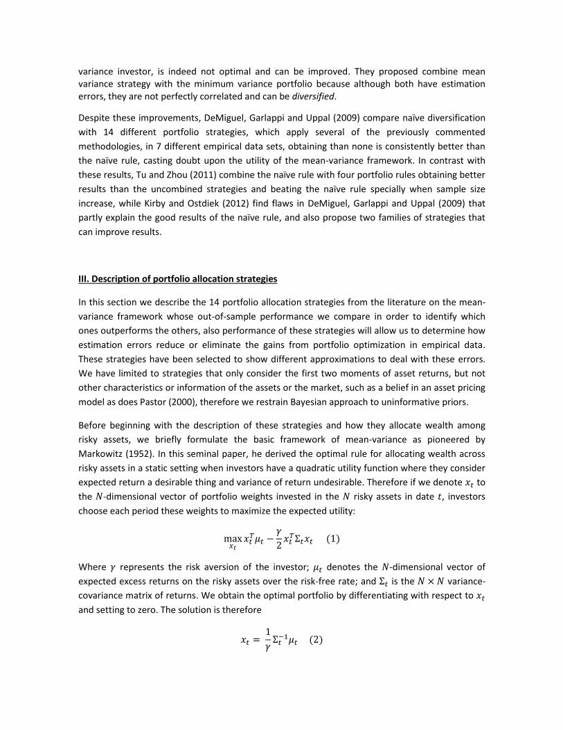
choose each period these weights to maximize the expected utility:

Where represents the risk aversion of the investor; denotes the -dimensional vector of

expected excess returns on the risky assets over the risk-free rate; and is the variance-

covariance matrix of returns. We obtain the optimal portfolio by differentiating with respect to

and setting to zero. The solution is therefore

Where is invested in the free-risk asset, and is an N-dimensional vector of ones.

Therefore, the relative weights in the portfolio with only risk assets are

| |

| |

We use this vector of relative weights in all the strategies to facilitate the comparison, note this is

equivalent to impose the following restriction to the optimization problem

∑

Where is the portfolio weight of asset on instant .

We group all the strategies in seven categories depending on their variation over this common

framework to deal with estimation risk. Table 1 lists them all.

Table 1: List of asset allocation strategies considered

# Strategy Code

Naïve diversification 1 1/N weights in all the risky assets ND

Sample-based mean-variance 2 Tangency portfolio TP

Bayesian-Stein shrinkage approach 3 Jorion strategy JR

Strategy with moment restrictions 4 Minimum variance MIN

Strategies with short selling constraint 5 Tangency portfolio without short selling TPC 6 Minimum variance without short selling MINC

Timing strategies 7 Volatility timing VT 8 Reward-to-risk timing RRT

Combination of strategies 9 Naïve with mean-variance strategy CMV

10 Naïve with mean-variance strategy without short selling CMVC 11 Naïve with minimum variance strategy CMIN 12 Naïve with minimum variance strategy without short selling CMNC 13 Three-fund strategy KZ 14 Naïve with three-fund strategy CKZ

This table lists the various mean-variance strategies considered. The last column shows a code

we use through the text to refer to the strategy.

III.A. Naïve diversification

The naïve (ND) strategy simply relies in allocate total wealth in equal parts between all the risky

assets, therefore its portfolio weights, as for each instant of time are, . Following

DeMiguel, Garlappi and Uppal (2009) we use this strategy as a benchmark for the other strategies,

because as they explain it is easy to implement because it does not rely either on estimation of the

moments of asset returns or on optimization, therefore no estimation risks are present, and

investors continue to use such simple allocation rules. Another important thing to notice is that it

never shorts any asset. Of course this strategy is not optimal as does not consider any information

to allocate wealth across assets, but as a benchmark let us know if active portfolio management

can outperform it, or estimation errors eliminate all potentials benefits from optimization.

III.B. Sample-based mean-variance

When moments of asset returns are known, Markowitz’s model lead to a portfolio allocation

where investor’s utility is maximized. This situation is not achievable in practice, when moments

are unknown and have to be estimated, generating estimation error. The simpler way to

implement his model is with the classic plug-in approach, by replacing moments of asset returns

on equation (2) and (3) with their sample counterparts and . This strategy does not take into

the account the effects of estimation errors and hence will show us their importance, because

with no such errors this strategy would outperform the rest of strategies that try to deal with

estimation errors, so any improvement of a strategy over this one are caused by them. As we only

consider the normalized portfolio, portfolio with only risky assets, we refer to this strategy as

tangency portfolio (TP), with weights of

| |

III.C. Bayesian-Stein shrinkage approach

Jorion (1986) tries to incorporate estimation risk into portfolio optimization by combining the use

of shrinkage and Bayesian estimators. For expected returns he proposed a shrinkage estimator to

minimize estimation errors over the sample mean. Based on the work of Stein (1956), the

estimator is obtained by shrinking the means toward a proposed common value that leads to a

decreased estimation error, so the estimator of expected returns is

( )

Where is the average excess return on the sample minimum variance strategy, and

represents the intensity of the shrinkage, therefore , and is calculated by

In which variance is estimated as proposed by Zellner and Chetty (1965),

.

For the variance-covariance matrix he used Bayesian estimation, which computes estimates by

using the predictive distribution of asset returns obtained by integrating the conditional likelihood

with respect to a subjective prior. So first, derives the predictive variance of asset returns using an

informative prior on with precision , and then uses sample estimates to arrive to the following

estimator:

(

)

Where

. With these estimators of the expected returns and variance, portfolios

weights are obtained the same way as the tangency portfolio in equation (3), hence this strategy is

the same as the previous one but with different estimators that deal with estimation error and

should perform better out-of-sample.

III.D. Strategy with moment restrictions

There is a general perception in the literature that estimation errors in expected returns affect

more to optimal portfolio weights that errors in the variance-covariance matrix, for example

Chopra and Ziembra (1993) conclude that, although depending on the investor’s risk dependence,

errors in expected returns generate at least three times the loss of errors in variance. Although

more recently, Kan and Zhou (2007) point out the importance of estimation errors in variance and

their interaction with errors in expected returns, so especially when the number of assets is large

relative to the number of periods of observed data, errors in the variance-covariance matrix have

an important role in the final outcome. Nevertheless, here we consider the minimum variance

strategy, where we ignore expected returns and only use the variance-covariance matrix to form

optimal portfolio weights. This would let us know if the sample mean is such an imprecise

estimator of population mean and the estimation error so large that not much is lost by ignoring it

when no further information about population mean is available.

We obtain the portfolio weights by solving this optimization problem

III.E. Strategies with short selling constraint

We consider two strategies that constrain short selling; specifically we consider the tangency

portfolio without short selling (TPC) and the minimum variance portfolio without short selling

(MINC). These strategies are obtained by imposing the following non-negativity constraint on the

portfolio weights in their optimization problems

Jagannathan and Ma (2003) showed for the minimum variance portfolio that not allowing short

selling is equivalent to modify the covariance matrix shrinking the larger elements of the matrix

towards zero, therefore two effects are generated. On the one hand, these large values could be

the consequence of estimation errors, hence constraining helps improving the estimation and

reducing their error. On the other hand, population covariance could be actually large, so we are

introducing specification error. The final outcome depends on the trade-off between estimation

and specification errors. But as proved by Frost and Savarino (1988), sample covariance-variance

matrix has large estimation errors, and in this case portfolio weight constraints are helpful as

Jannagathan and Ma (2003) confirmed. DeMiguel, Garlappi and Uppal (2009) document that for

the mean variance portfolio this constraint is also a form of shrinkage on the expected returns

towards the average, and as before the net effect depends on the trade-off between estimation

and specification errors. Also, Lozano (2013) finds that in general, this short selling restriction in

the minimum variance strategy imitates the naïve diversification out-of-sample performance

which is a sub-optimal strategy but without estimation errors, therefore this constraint is a way of

limitation of the estimation errors rather than improving the benefits of diversification.

III.F. Timing strategies

Kirby and Ostdiek (2012) introduced two classes of active portfolio strategies that try to retain the

principal benefits of naïve diversification, they do not do an optimization; variance-covariance

matrix is not inverted; and there is no short selling. However, they use sample information to

determine portfolio weights, specifically both rely in return volatilities and a tuning parameter that

allows some control over portfolio turnover and therefore their transaction costs, while their

difference lay in the use or not of expected returns.

1. Volatility timing (VT)

In their first strategy, portfolio weights on each asset are calculated by

( ⁄ )

∑ ( ⁄ )

Where is the asset sample return variance and measures timing aggressiveness with .

This can be seen as a form of minimum variance portfolio where the correlations of asset returns

are considered to be zero. This of course is not the case, but reducing /2 the number of

parameters to be estimated could lead to reduced estimation errors that can outweigh the

information loss. The parameter determines how aggressively portfolio weights are adjusted in

response to volatility changes. As Kirby and Ostdiek (2012) explain, if it tends to zero we get the

naïve diversification, and when tends to infinity the weights on the asset with less variance

approaches to one. We set this value to 2 because they show that values over 1 help to

compensate for the loss caused by ignoring the correlations and is middle ground between the

values they used.

2. Reward-to-risk timing (RRT)

This strategy tries to improve VT by incorporating information of expected returns, although as

previously stated, they are estimated with less precision than variances and would lead to an

increase in estimation errors. So, in this case portfolio weights for asset are

(

⁄ )

∑ (

⁄ )

With denoting expected return of asset and . We use

because first in

this strategy we do not want to allow short selling as would happen if expected returns are

negative for some assets, and second these negative returns can also cause the denominator of

the equation to be close to zero, generating extreme weights and high turnover. So we assume

that the investor has a strong prior belief that .

III.G. Combination of strategies

Finally we consider a series of strategies that are a combination of other strategies already

presented. Tu and Zhou (2011) compare four asset allocation strategies and their respective

combination with the naïve diversification, trying to determine if these combinations outperform

their uncombined components. A combination can be interpreted as a shrinkage estimator applied

to portfolio weights with naïve diversification as the target. Optimization strategies weights are

asymptotically unbiased by have an important variance, especially in small samples, on the

contrary naïve diversification is biased and will not converge to the optimal weights but has no

variance, as weights are not change over time, therefore a combination can be interpreted as a

trade-off between bias and variance. In theory, as Tu and Zhou proved, an optimal combination

rule exists and can be determined analytically, being this optimal combination, which minimizes

the expected loss of mean variance investor’s utility, defined as:

[ ]

Where is the mean variance investor’s utility in-sample, so is optimal, and [ ] is the

expected utility of the combination strategy. The combination strategy is then:

With being the weights of the strategy we combine with the naïve.

In practice, it has to be estimated, but as only one parameter is estimated errors should be small

and their advantages remain. We first describe four combinations rules with naïve diversification

and already commented strategies, and then the three-fund strategy defined by Kan and Zhou

(2007) and its combination with naïve diversification.

1. Naïve with mean-variance strategy (CMV)

Following Tu and Zhou (2011) we combine naïve diversification with mean variance strategy.

Analytically they proved that the estimated optimal combination is:

( )

Where

And represents the weights of mean variance strategy, is the estimator of the impact from

the bias of naïve diversification, and measures the impact from the variance of mean variance

strategy.

is the estimator of the square Sharpe ratio given by Kan and Zhou (2007)as:

( ) ( )

( )⁄ ⁄ ⁄

Where

∫

Is the incomplete beta function and is the sample square Sharpe ratio:

Eventually, as we use relative weights in all of the strategies, we normalize the weights as:

| |

2. Naïve with mean-variance strategy without short selling (CMVC)

We also combine naïve diversification with mean variance when short selling is not allowed. For

this strategy we use the same combination coefficient as defined in equation (16), this way,

improvements over the former strategy will be determined solely due to this restriction. So

( )

And after normalization

| |

3. Naïve with minimum variance strategy (CMIN)

As DeMiguel, Garlappi and Uppal (2009) we consider a combination between naïve diversification

and minimum variance strategy. As explained when commenting about minimum variance

strategy, the reason is the difficulty of estimating expected returns, so the loss of ignoring their

information could be outperformed by the reduction of estimation errors. The strategy considered

is:

( )

Where is chosen to maximize the expected utility of the mean variance investor, but as we are

not considering expected results of asset returns it is equivalent to minimize the variance of the

combination, resulting in:

(

)( )

( )(

)

4. Naïve with minimum variance strategy without short selling (CMNC)

In this case, we present a new strategy by combining naïve diversification with minimum variance

when short selling is not allowed. We reutilize from equation (27) to see if constraining short

selling improves performance in combination strategies. Its results would help understand if using

multiple approaches to reduce estimation errors help, or so many restrictions hamper

performance because of specification errors. The strategy is therefore:

( )

5. Three-fund strategy (KZ)

Kan and Zhou (2007) proved analytically that while a portfolio with the risky asset and the

tangency portfolio is optimal in-sample that is not the case out-of-sample when moments have to

be estimated and the tangency portfolio is obtained with estimation error. Therefore, they

propose a new three-fund strategy by adding the minimum variance as a way to diversify

estimation error, because while the minimum variance also has estimation error, their errors are

not perfectly correlated. They consider the non-normalized weights of this strategy to be:

(

)

Where and are constants to be chosen optimally, by maximizing the expected out-of-sample

mean variance investor’s utility, resulting in:

(

)

(

)

With

( ) ( )

( )⁄ ⁄⁄

( ) ( )

Where is the sample expected excess return of the ex-ante minimum variance strategy, and

is an unbiased estimator of the square slope of the asymptote to the ex-ante minimum variance

frontier. Finally we normalize, so the risky assets weights are:

| |

6. Naïve with three-fund strategy (CKZ)

Following Tu and Zhou (2011) we combine the three-fund strategy with naïve diversification. It is

important to note that in this case we are making a combination with a strategy that is already a

combination of strategies, so it could show if combining a higher number of strategies could be

beneficial or the more coefficients that need to be estimated can lead to more estimation errors

that worsen performance. In this case, the risky assets weights are:

( )

Estimated optimal combination is obtained by:

With given by equation (17), and where:

([ ( )

]

[ ( )

])

(

)

With defined in equation (20), in (19), in (35) and in (34).

IV. Data

In this section we describe the portfolios and periods of time used in this dissertation for the

empirical analysis. The ten empirical datasets are listed in Table 2.

Table 2: List of datasets

# Countries Portfolios N Code

1 Spain and Italy From each country, 2 portfolios sorted by book-to-market and the market portfolio

6 BM2 2 BM2 plus Belgium and France 12 BM4 3 BM4 plus Germany and Netherlands 18 BM6 4 BM6 plus Norway and Sweden 24 BM8 5 BM8 plus Switzerland and United Kingdom 30 BM10

6 Spain and Italy From each country, 2 portfolios sorted by earnings-price and the market portfolio

6 EP2 7 EP2 plus Belgium and France 12 EP4 8 EP4 plus Germany and Netherlands 18 EP6 9 EP6 plus Norway and Sweden 24 EP8 10 EP8 plus Switzerland and United Kingdom 30 EP10

This table lists the datasheet used. Datasets consists on monthly excess returns over the one-month German

bill. N is the number of assets. Abbreviations will be used to refer to these datasets in the tables. All datasets

span from January 1975 to December 2012.

The data we use consists of monthly excess returns over the risk-free asset on equity portfolios of

10 European countries obtained from Kenneth French’s website3. We use European data because

literature in out-of-sample performance based on mean-variance framework has been mainly

focused in the United States and this will allow us to compare both markets and establish if

conclusions about the performance of different strategies in the US are kept in Europe, or an

investor should apply a different strategy depending in its investment countries. Country selection

has been based basically by the availability of data, and includes the more liquid markets in

Europe, in and out the euro zone.

3 http://mba.tuck.dartmouth.edu/pages/faculty/ken.french/data_library.html

For each country we have 2 portfolios sorted by book-to-market ratio (firms in top 30% and in

bottom 30%), other 2 sorted by earnings-price ratio (same as previous) and a market portfolio.

With this we create 10 different data sets, 5 with the book-to-market portfolios and 5 with

earnings-price the following way. We take the market portfolio and the 2 portfolios sorted by

book-to-market from Spain and Italy for a total of 6 portfolios; that is our first data set. To the

previous data set we add the same portfolios from Belgium and France totaling 12 portfolios; the

second data set. We continue this way adding Germany and Netherlands; Norway and Sweden;

Switzerland and United Kingdom to form the third, fourth and fifth data sets. Each pair of

countries has been selected based on their similar financial markets characteristics, leaving for the

last two, the more important European markets outside the euro zone. To make the other five we

simply change the book-to-market portfolios with earnings-price portfolios. Different statistics of

these data are shown in Table 3. Changing datasets by adding a pair of countries allow us to

observe the performance of each strategy with different number of assets, so we have portfolios

ranging from 6 to 30. In-sample we know the returns and risk of every asset, hence there is no

doubt that a higher number of assets improve performance, as diversification improves with more

assets. But this is not always the case out-of-sample, because there are an increasing number of

moments of the returns to be estimated, therefore estimation errors also grow which could end

with a worse performance of an optimization strategy when increase.

As risk-free asset we use the one-month German bill obtained from Datastream. This was daily

data and was annualized so we turned it into monthly data by taking the mean of all the days in

each month and removing the annualization.

Our data span from January 1975 to December 2012, the longest period for which we have data

for all the countries analyzed. This covers a time frame which includes the current European debt

crisis and therefore our findings can also contribute to the understanding of the crisis in the

portfolio performance, also includes the introduction of the euro in 6 of the 10 countries

considered. We calculate our measures, such as Sharpe ratio, in two ways. Firstly, we calculated

them for the whole period, with a length, , of 456 months. Secondly, for a series of sub-periods,

where each sub-period has a length of 300 months with the first one ranging from January 1975 to

December 1999. Then we move the initial and final date one month ahead to form all the other

sub-periods until the last one which is from January 1988 to December 2012, for a total of 157.

Figure 1 shows the difference between considering the whole period, classic evaluation

performance, and use different sub-periods. This second approach will allow us to compare their

evolution over time, so would help us to evaluate the performance stability through time. Thus,

conclusions regarding strategies comparisons would be robust in the sense that they are evaluated

not only in one single T, but in a subsequent number of periods. Also, this approach will allow us to

evaluate how different results are achieved by changing 2 data at a time, which has not been

previously tested at least in historical data sets. Studying characteristics from such periods would

let us know reasons for this performance. Also, for each strategy we can compare its results over

time for different number of assets, and again search in the data for the cause.

Figure 1: Classic and sub-periods portfolio evaluation performance

Classic portfolio evaluation performance:

One out-of-sample performance measure by dataset and strategy.

Sub-periods portfolio evaluation performance:

157 out-of-sample performance measures by dataset and strategy.

Adapted from Lozano (2013).

Table 3 show a list of basics statistics from all the datasets we use in the present work. Obviously,

when the same countries are considered, statistics from book-to-market and earning-price

portfolios are very similar as markets portfolios are present in both BM and EP, and the other

portfolios are formed with some assets in common. But some facts still emerge. First, the

portfolios form with only Spain and Italy assets has the smallest mean and highest variance,

therefore strategies’ performances of BM2 and EP2 should be inferior. Second, from the minimum

correlation results it can be seen that all the assets have a positive and considerable pairwise

correlation, which is in no case lesser than 0.3. Third, correlation range, which is the difference

between the maximum and the minimum correlation, is a bit bigger in BM than in EP. A bigger

correlation range means that assets are more different as varied correlations imply various

responses to changes in each asset, so a strategy should perform better in this case, in our case in

BM, as variance can be more adequately minimized. And forth, from maximum and minimum

return value it can be seen important changes in both directions of assets performance, which can

result in significant differences between strategies depending on their portfolio weights.

Performance

measure

Dataset

Matrix (TxN)

Out-of-sample

strategy return vector

Performance

measure 1

The first dataset goes from Jan 1975 to Dec 1999, and the last

from Jan 1988 to Dec 2012.

Performance

measure 157

Table 3: Data statistics

BM2 BM4 BM6 BM8 BM10 EP2 EP4 EP6 EP8 EP10

Mean 0.0054 0.0071 0.0075 0.0080 0.0081 0.0060 0.0073 0.0074 0.0081 0.0081

Standard Deviation 0.0773 0.0721 0.0696 0.0725 0.0706 0.0762 0.0715 0.0694 0.0722 0.0702

Max. Correlation 0.9654 0.9654 0.9654 0.9654 0.9678 0.9502 0.9568 0.9568 0.9568 0.9715

Min. Correlation 0.4749 0.3653 0.3653 0.3270 0.3174 0.4760 0.4385 0.4051 0.3479 0.3479

Correlation Range 0.4905 0.6001 0.6001 0.6384 0.6504 0.4742 0.5183 0.5517 0.6089 0.6236

Max. Return Value 0.4040 0.5398 0.5398 0.5398 0.5431 0.5333 0.5333 0.5333 0.5333 0.5431

Min. Return Value -0.3175 -0.3175 -0.3565 -0.3771 -0.3771 -0.3303 -0.4512 -0.4512 -0.4512 -0.4512

This table lists basics statistics of the 10 different datasets used, as shown in Table 2. Correlation Range is defined as

(Max. Correlation – Min. Correlation).

V. Measures to evaluate performance

This section describes the methodology and measures we use to determine the performance of a

series of asset allocation strategies. We follow the procedure adopted by DeMiguel, Garlappi and

Uppal (2009).

As them we use a rolling-sample approach. This means that for each T-month period of asset

returns, we use an estimation window of length , in our case , to estimate the

parameters needed by all the strategies. So, starting in we estimate these parameters

with the returns from the previous months. With these estimates each strategy determines its

optimal portfolio weights, and with them we can calculate the out-of-sample return of the next

month. We continue this process by moving one month ahead until we reach the end of the

period, ending with a series of out-of-sample returns for each strategy.

With these out-of-sample returns we calculate four measures to determine the out-of-sample

performance of each strategy. These measures are Sharpe ratio, certainty equivalent, turnover

and return-loss.

V.A. Sharpe ratio

The out-of-sample Sharpe ratio of a strategy is defined as the mean of excess returns over their

sample standard deviation:

An investment is only good when higher returns do not come with too much additional risk, so the

Sharpe ratio can be considered as a measure of risk-adjusted performance.

V.B. Certainty equivalent

The out-of-sample certainty equivalent return of a strategy is calculated as the utility function of

a mean variance investor:

Where represents the investor’s risk aversion, in our case equals 1, the same value DeMiguel,

Garlappi and Uppal (2009) use, in order to be able to compare results. It is called certainty

equivalent return because represents the free-risk rate in which the investor would be indifferent

between adopting strategy and staying with the risk-free asset.

V.C. Turnover

The turnover shows the amount of trading required to implement a strategy, and is defined as the

average sum of the trades in the N assets:

∑ ∑(| |)

Where is the desired portfolio weight under strategy in asset at time after

rebalancing, while is the portfolio weight at time but before rebalancing. Therefore

the term in brackets represent the trades on each asset in each period in absolute value.

For naïve diversification we calculate its absolute turnover, while for the other strategies we

report their turnover relative to the naïve diversification.

V.D. Return-loss

Related to the turnover, we show how transaction costs affect the returns of each strategy via

turnover. Following DeMiguel, Garlappi and Uppal (2009) we set the cost of a transaction to 50

basis points and denoted it by .

First, we define the return from strategy before rebalancing as: ∑ . As said

before, when the portfolio is rebalanced at it generates trades of each asset of value

| |. Therefore the total transaction costs in each instant of time are the sum of

this trades for all the assets multiply for the cost of a transaction, . So, wealth for strategy k

evolves as follows:

( )( ∑| |

)

The return net of transactions costs of the strategy on instant is then:

.

With this series of net returns, we can calculate the return-loss of a strategy with respect to naïve

diversification, as the additional return a strategy need to perform as well as the naïve in terms of

Sharpe ratio. Defining and are the monthly out-of-sample mean and standard deviation of

the net returns of naïve diversification, while and are the corresponding parameters for the

strategy . Then, the return-loss for the strategy is:

VI. Results for the whole period

In this section we compare the out-of-sample performance of all the strategies considered during

the whole period, therefore .

VI.A. Sharpe ratio

Panel A from Table 4 and Table 5 include the Sharpe ratio results of the 14 strategies in the two

European data portfolios for different number of assets and countries as defined in Table 2. The

first row shows the results of the naïve strategy, it can be seen that, in general, that Sharpe ratio

improves as the number of assets increase from 0.1298 to 0.1670. As we will see, as grows there

are two opposite effects that affect the Sharpe ratio. On the one hand, it increases the benefits of

diversification. On the other, it enlarges the estimation errors because more parameters have to

be estimated. In the naïve strategy there is no such estimation therefore the results are

unaffected by these errors. It should be noted that the greater improvement comes when we

increase from 6 to 12, showing how the more important benefits from diversification comes

when we add France and Belgium portfolios to the ones of Spain and Italy, from Table 3 we know

that portfolios from the later have a higher mean and lesser variance, thus explaining this

important increase in Sharpe ratio. These results are quite similar of the ones obtained by

DeMiguel, Garlappi and Uppal (2009) ranging from 0.1277 to 0.1876, except for their Fama and

French data set with a Sharpe ratio with a Sharpe ratio of 0.2240, but this is a portfolio with only

three assets, hence performance is quite similar in European and US markets.

The remaining rows show the Sharpe ratio of the rest of strategies. First, looking for general

results, we can note that in the book to market data portfolios all the strategies outperform the

naïve when , with the exceptions of the combination of the naïve and the 3 fund strategy

and the tangency portfolio, but as rises these number of outperformers is reduced down to 5

when , as a result of the increasing estimation errors consequence of a higher number of

parameters to estimate which reduce and in some cases eliminate the benefits of optimization as

opposed to naïve diversification. In the earnings-price data portfolios, only 8 strategies have a

higher Sharpe ratio than the naïve when , but 5 of them maintain this improvement for all

the combinations of countries analyzed. Therefore, the number of assets is in fact important, as

grows more parameters have to be estimated, this generates bigger estimation errors that

worsens Sharpe ratios on the optimization strategies, as opposed to naïve diversification which

maintains its portfolio weights not been affected by estimations, explaining why more strategies

are outperformed by naïve diversification when the number of assets increase.

Table 4: Out-of-sample performance in book-to-market portfolios

Strategy BM2 BM4 BM6 BM8 BM10

Panel A: Out-of-sample Sharpe Ratio

1/N 0.1298 0.1579 0.1620 0.1641 0.1670 TP 0.1257 0.0797 0.0169 0.0743 0.0519 CMV 0.1318 0.1896 0.1371 0.1313 0.1164 TPC 0.1485 0.1493 0.1113 0.1140 0.1144 CMVC 0.1358 0.1753 0.1692 0.1647 0.1661 MIN 0.1737 0.2431 0.2418 0.2392 0.2252 KZ 0.1465 0.1847 0.0880 0.1840 0.1350 CMIN 0.1556 0.2045 0.2081 0.2066 0.2007 CKZ 0.0792 0.1198 0.1464 0.1528 0.1603 MINC 0.1591 0.2143 0.2182 0.2158 0.2035 CMNC 0.1456 0.1877 0.1918 0.1886 0.1815 VT 0.1401 0.1738 0.1752 0.1771 0.1802 RRT 0.1473 0.1707 0.1668 0.1647 0.1633 JR 0.1461 0.1436 0.0471 0.1270 0.0821

Panel B: Out-of-sample Certainty Equivalent

1/N 0.645% 0.765% 0.772% 0.793% 0.780%

TP 0.778% 0.003% -4.218% -0.145% -3.225%

CMV 0.722% 1.160% 0.803% 0.691% 0.563%

TPC 0.830% 0.770% 0.534% 0.567% 0.560%

CMVC 0.690% 0.880% 0.816% 0.795% 0.779%

MIN 0.935% 1.200% 1.150% 1.145% 1.011%

KZ 0.823% 1.028% 0.375% 0.983% 0.823%

CMIN 0.809% 0.991% 0.957% 0.952% 0.846%

CKZ 0.212% 0.562% 0.708% 0.749% 0.751%

MINC 0.835% 1.043% 0.994% 0.976% 0.878%

CMNC 0.745% 0.904% 0.885% 0.872% 0.796%

VT 0.711% 0.837% 0.814% 0.826% 0.792%

RRT 0.781% 0.849% 0.805% 0.794% 0.759%

JR 0.865% 0.876% -0.610% 0.753% -0.033%

Panel C: Out-of-sample turnover

1/N 0.0265 0.0278 0.0275 0.0310 0.0301 TP 126.765 436.217 1327.41 315.093 1059.65 CMV 32.8959 50.0567 79.8858 63.1568 66.0142 TPC 3.3771 6.4724 8.8771 8.3911 8.1827 CMVC 3.2360 3.7809 3.9507 3.1159 2.5965 MIN 9.1309 15.7049 23.1555 26.9761 36.3444 KZ 30.1341 84.6373 129.025 53.4541 192.537 CMIN 4.8512 7.2814 9.9089 10.4781 12.9567 CKZ 608.246 13.1527 13.9129 8.5298 9.1358 MINC 2.4457 3.2910 3.1070 2.9036 3.6546 CMNC 1.8233 2.0223 1.9066 1.6987 1.9384 VT 1.2350 1.2203 1.2104 1.1458 1.1565 RRT 3.1325 3.0912 3.0580 2.8261 3.0022 JR 41.9151 189.694 249.854 104.035 447.824

Panel D: Out-of-sample Return-loss

TP 1.587% 14.827% 10.498% 5.405% 39.445%

CMV 0.380% 0.505% 1.319% 1.232% 1.371%

TPC -0.104% 0.176% 0.537% 0.497% 0.508%

CMVC -0.005% -0.044% 0.020% 0.048% 0.039%

MIN -0.161% -0.232% -0.088% 0.007% 0.249%

KZ 0.154% 1.027% 2.196% 0.645% 5.236%

CMIN -0.104% -0.146% -0.093% -0.055% 0.038%

CKZ 7.881% 0.384% 0.263% 0.174% 0.140%

MINC -0.167% -0.284% -0.254% -0.229% -0.144%

CMNC -0.089% -0.147% -0.135% -0.107% -0.059%

VT -0.068% -0.096% -0.073% -0.071% -0.068%

RRT -0.106% -0.069% -0.007% 0.017% 0.040%

JR 0.294% 4.228% 4.528% 1.867% 18.149%

This table lists the results from measures defined in section V for the 14 mean-variance strategies described in

section III for the book-to-market portfolios. Values for certainty equivalent and return loss are shown in

percentage points.

Table 5: Out-of-sample performance in earnings-price portfolios

Strategy EP2 EP4 EP6 EP8 EP10

Panel A: Out-of-sample Sharpe Ratio

1/N 0.1299 0.1540 0.1521 0.1598 0.1629

TP 0.0673 -0.0369 -0.0385 -0.0543 -0.0398

CMV -0.0233 0.1076 0.0525 0.0961 0.0828

TPC 0.1468 0.1455 0.1182 0.1146 0.1069

CMVC 0.1330 0.1625 0.1544 0.1629 0.1613

MIN 0.1659 0.1946 0.1957 0.2003 0.2179

KZ 0.0751 0.0004 0.0130 -0.0528 -0.0298

CMIN 0.1400 0.1706 0.1720 0.1745 0.1868

CKZ -0.0489 0.1286 0.1370 0.0853 0.1064

MINC 0.1639 0.1942 0.1969 0.1970 0.1940

CMNC 0.1408 0.1721 0.1736 0.1750 0.1733

VT 0.1407 0.1687 0.1617 0.1662 0.1709

RRT 0.1406 0.1667 0.1550 0.1609 0.1613

JR 0.0736 -0.0178 -0.0164 -0.0537 -0.0356

Panel B: Out-of-sample Certainty Equivalent

1/N 0.647% 0.744% 0.719% 0.769% 0.758%

TP -7.202% -8.855% -9.310% -12972.300% -143.365%

CMV -3.544% 0.537% -0.017% 0.460% 0.325%

TPC 0.809% 0.758% 0.576% 0.563% 0.508%

CMVC 0.678% 0.791% 0.735% 0.784% 0.751%

MIN 0.905% 0.952% 0.952% 0.978% 0.979%

KZ -0.829% -1.253% -0.905% -1280.130% -27.783%

CMIN 0.719% 0.815% 0.804% 0.813% 0.790%

CKZ -12.157% 0.632% 0.688% -1.499% 0.561%

MINC 0.879% 0.940% 0.930% 0.927% 0.845%

CMNC 0.722% 0.827% 0.816% 0.825% 0.763%

VT 0.720% 0.809% 0.754% 0.780% 0.757%

RRT 0.738% 0.813% 0.729% 0.769% 0.746%

JR -1.325% -2.768% -2.842% -3946.100% -54.511%

Panel C: Out-of-sample turnover

1/N 0.0263 0.0274 0.0274 0.0309 0.0300

TP 2092.64 571.866 600.990 9420.19 5366.57

CMV 125.260 56.1805 103.872 77.1794 103.939

TPC 2.8407 8.4275 7.8674 8.0977 8.7493

CMVC 3.5901 3.6903 4.0759 3.5337 3.0968

MIN 8.7856 14.6770 22.3098 25.7626 34.2017

KZ 277.754 146.198 161.028 146.328 3165.59

CMIN 4.0304 5.9121 9.3556 9.9242 11.9089

CKZ 2980.53 19.2294 27.6870 47.6895 129.626

MINC 3.4399 3.8552 3.6912 3.3752 4.2395

CMNC 2.1331 2.0096 2.0316 1.8649 2.0523

VT 1.2471 1.1912 1.2099 1.1502 1.1619

RRT 2.7751 2.8912 3.0141 2.7997 2.9485

JR 440.538 323.098 255.809 393.221 5287.22

Panel D: Out-of-sample Return-loss

TP 100.041% 28.863% 8.283% 104.855% 215.699%

CMV 2.706% 1.206% 2.219% 1.638% 2.245%

TPC -0.091% 0.215% 0.364% 0.434% 0.479%

CMVC 0.034% 0.008% 0.043% 0.029% 0.046%

MIN -0.151% -0.019% 0.091% 0.170% 0.247%

KZ 5.591% 3.311% 3.093% 5.089% 156.981%

CMIN -0.028% -0.009% 0.029% 0.077% 0.071%

CKZ 4.905% 0.421% 0.547% 0.298% 2.762%

MINC -0.199% -0.188% -0.209% -0.161% -0.072%

CMNC -0.057% -0.089% -0.105% -0.068% -0.021%

VT -0.072% -0.086% -0.053% -0.035% -0.040%

RRT -0.043% -0.055% 0.012% 0.017% 0.034%

JR 6.752% 15.644% 4.494% 31.836% 94.680%

This table lists the results from measures defined in section V for the 14 mean-variance strategies described in

section III for the earnings-price portfolios. Values for certainty equivalent and return loss are shown in

percentage points.

Now, looking for more specific results, the higher results for both book-to-market and earnings-

price portfolios belong to the minimum variance strategy with a maximum of 0.2431 in BM4, a

nearly 40% increase over ND, in DeMiguel, Garlappi and Uppal (2009) MIN only outperforms ND in

four of six datasets and their Sharpe ratios are heterogeneous, from a maximum of 0.2778 to a

minimum of -0.0183 depending on the datasets, so when we choose portfolio weights via

optimization out-of-sample performance depends deeply in the risky assets used to form the

portfolio. The other strategies that consistently outperform the naïve in both portfolios are the

minimum variance without short selling, their combinations with the naïve and the volatility

timing strategy, with Sharpe ratios 10% or 20% over ND. Looking for the cause of this outcome, it

is important to note that all of them have in common restrictions on the estimation of the

moments of asset returns, instead of using the expected returns and the sample covariance matrix

to determine their portfolio weights as the mean variance strategy does, they ignore the estimates

of expected returns and only use the estimate of the covariance of asset returns. Therefore, a first

important conclusion is the beneficial effects of these restrictions out-of-sample as opposed to in-

sample due to the estimation errors. We can also see that the best Sharpe ratio corresponds to

simply ignore expected returns, so restraining short selling as MINC, making a combination with

naïve diversification, CMIN and CMNC, or ignore the estimates of the correlations, VT, generates a

loss in Sharpe ratio.

Two other strategies that improve naïve diversification, except when we consider all 10 countries,

are the combination of the naïve and mean variance without short selling, and the reward-to-risk

strategies, but this gains over ND are insignificant. RRT is like VT except that the estimates of

expected returns are used to choose portfolio weights. Sharpe ratios are worse in RRT, therefore

the estimations of expected returns do not help to achieve a better Sharpe ratio, as a consequence

of higher estimation errors. As opposed as before, CMVC improves over MVC, so combine a

strategy with the 1/N rule can achieve better results when the uncombined strategy does worse

than naïve diversification, as Tu and Zhou (2011) proved.

On the other hand, the worst performance is from the tangency portfolio that has a worse

performance than naïve diversification in all the data, and even has negative Sharpe ratios in four

of the EP portfolios, similar to the results obtained by DeMiguel, Garlappi and Uppal (2009). This

strategy does not deal with estimation errors and is optimal in-sample, showing the importance of

trying to reduce estimation errors. The combination of the naïve and the 3 fund strategy also has a

worse performance than the naïve in all the data. The use of a Bayesian estimator, as in Jorion

strategy it leads to the minor improvement over the tangency portfolio of all its modifications to

account for estimation errors, and therefore is still outperformed by the naïve strategy. This

strategy use modified expected returns and covariance matrix but is otherwise identical to the

tangency portfolio strategy, so this modification is the less effective of the studied. Another

modification of the tangency portfolio as constraining it by no allowing short selling gets better

Sharpe ratio than the 1/N rule, but only when the number of assets is 6, but in any case improves

tangency portfolio performance.

In an intermediate position are the rest of combinations between two portfolios. Here we can see

a different performance in the data portfolios. The combination of the naïve and the mean

variance portfolio does particularly well in the book-to-market data portfolios when is small but

not in the earn-to-price data portfolios, this is a consequence of tangency portfolio also

performing better in the book-to-market data sets. Mean-variance methodology is optimal in-

sample, but not necessarily out-of-sample. This loss in out-of-sample performance is caused by

estimation errors and therefore its value depends on its magnitude, thus we can conclude that

estimation errors are more important in the earn-to-price data portfolios. This performance

depending on the data is also true for the three fund strategy and in the same way, while the

remaining strategies show a similar trend in both cases but with higher Sharpe ratios in the book-

to-market data portfolios, especially for the higher values as in the minimum variance strategy.

From these results and the previous combinations, we can conclude that the combination of

portfolios is particularly helpful when we combine the mean variance portfolio with another

portfolio, but not so much when we combine the minimum variance with the naïve. The reason is

because in the former we are introducing restrictions on the moments, because part of the

resulting portfolio is the naïve strategy which does not consider the estimation of moments,

therefore the performance improves as the estimation of parameters, and hence their errors, only

account for a part of the selected portfolio, and this errors are quite important in the mean

variance methodology as the performance of the tangency portfolio proves.

As a conclusion, we have seen that all the methodologies implemented to account for estimation

errors, such as combining portfolios or constraining short selling, improve the out-of-sample

Sharpe ratio when adopted individually, being ignoring the estimates of the expected returns

which achieves better results. But adding a second methodology does in general reduce the

Sharpe ratio.

Finally, if we discussed the evolution of the strategies as the number of countries increases, for

most of them in the book-to-market data portfolios have the biggest Sharpe ratio when only

Spain, Italy, France or Belgium are considered or at most when we add Germany and Netherlands,

and only the volatility timing strategy has a big and increasing result as does . That is because a

higher number of assets involves a higher number of parameters to be estimated which leads to

an increase in the estimation errors and therefore the advantages of the diversification are

eliminated. Not surprisingly, the volatility timing strategy is the one that not only ignores the

estimation of expected returns but also the correlations, therefore reducing the number of

parameters to be estimated. Also, BM8 and BM10 include Sweden and Norway, whose portfolios

have higher standard deviation helping to explain this reduction in performance. On the contrary,

in the earnings-price data portfolios, more strategies perform better as increases, which should

be consequence of lesser estimation errors and as Table 3 show, the increased in variance from

portfolios in Sweden and Norway is accompanied by an important increase in mean.

VI.B. Certainty equivalent

Panel B of Table 4 and Table 5 show the certainty equivalent results from all the strategies.

Obviously, they are similar to the previous Sharpe ratios, a fact already observed in the literature,

as in both measures higher mean returns implies a higher value as does a lesser variance, standard

deviation in the case of the Sharpe ratio. We have set the risk aversion, gamma, to 1 as DeMiguel,

Garlappi and Uppal (2009) does to allow comparison. A higher risk aversion would penalize more

the variance of the returns.

As before, the first row shows the results of the naïve strategy. It continues to grow as the number

of assets increase especially between 6 and 12 assets when passes from 0.645% to 0.765%, again

due to Spain and Italy having a lesser mean and higher variance than the rest of countries, but

unlike in the Sharpe ratio, here when , the certainty equivalent is reduced in both data

portfolios, so the increase in the variance of the returns surpasses the increments of the returns

means. This fact is, as expected, shared by the other strategies as naïve diversification tends to

have lesser variance in the returns because do not change its portfolios weights based on

estimations looking for an optimal outcome.

Once again, in the book-to-market data portfolios, the strategies outperform the naïve when we

consider only Spain and Italy but six do it when we use portfolios from all the ten countries. In the

earnings-price data portfolios less strategies improves the certainty equivalent of naïve

diversification, and only three, MIN, MINC and CMIN does for all the number of assets studied.

Then we can conclude that optimization works better in the book-to-market portfolios due to a

bigger correlation range, as shown in Table 3, which improves the benefits of diversification as

assets evolve more different, and that variance of the returns grows with the number of assets

removing the benefits of this optimization.

The minimum variance portfolio continues to be the best strategy based on certainty equivalents

results. Other strategies with good results are MINC and CMIN, which also beat naïve optimization

in all the cases considered, and CMNC, VT which only are worse than the 1/N rule when in

the earnings-price portfolios. These best five strategies coincide with the best in Sharpe ratio

performance, so restrictions on the moments of returns are also the best way to achieve a high

certainty equivalent value.

The worst results correspond to TP, CKZ and JR. TP and JR, apart from being outperformed by

naïve diversification in the majority of situations, achieve extremely negative ceq values in some

occasions. These two strategies have in common the use of the mean variance methodology

without restrictions, confirming the need for methodologies that reduce the estimation errors.

The tangency portfolio without short selling and the rest of combinations stay in middle ground,

beaten naïve diversification when is small, but failing when is big. CMV and KZ do a better

performance in the book-to-market portfolios, something that was also true in their Sharpe ratios

and demonstrate the important link between these two measures. About combining a strategy

with the naïve, it contributes to an improvement when the strategy alone performs worse than

naïve diversification but not when the opposite happens, resulting in ceq values generally between

its two components.

Lastly, we comment on the evolution of the strategies when the number of assets increases. The

best ceq results occurs mostly when in the book-to-market portfolios, but this pattern is

not maintain in the earnings-price portfolios varying between strategies, although if we focus on

the best strategies we can say that and provide the greatest ceq values. Therefore

we can conclude that a higher number of assets involve more parameters and increased estimator

errors harming diversification’s benefits.

VI.C. Turnover

Panel C from Table 4 and Table 5 show the turnover of all the strategies in both data portfolios

and different number of assets. The turnover of the naïve strategy in the first row is an absolute

value, showing an upward trend as the number of assets increase and similar values in both data

portfolios. These turnovers are small because in this strategy the weight on each asset is always

1/N, so turnover is only generated by changes in asset prices, not by optimization decisions, and

are similar of those obtained by DeMiguel, Garlappi and Uppal (2009), while for the optimization

strategies results vary between ours datasets and theirs, and also among datasets considered by

them, especially for strategies with higher turnovers. Once again data affects greatly strategies

performance.

The turnovers for all the others are relative to naïve diversification and are always bigger than 1

due to active portfolio management. Before commenting the results, we should note that if

transaction costs are not taken into account a high turnover should not affect, in principle, the

performance of a strategy and would only show its aggressiveness changing asset weights to

maximize the utility of the investor. But as we introduce transaction costs, higher returns are

needed as turnover increases to compensate these extra costs.

The highest turnovers correspond to TP, JR, CKZ, KZ and CMV. These strategies share the presence

of an unrestricted form of the mean variance methodology, optimizing with the estimations of

means and variances of returns, therefore more estimations and parameters that decide changes

in the portfolio weights. Also, these do not have any restriction. Both things explain these large

turnovers. They also have great variations with different number of assets and not homogeneous

patterns between data portfolios, for example, more extreme values in the earnings-prices

portfolios especially when and . None of these strategies do particularly when in

the Sharpe ratio and ceq results.

The winning strategy with respect to Sharpe ratio and certainty equivalent, minimum variance

portfolio, has intermediate turnover. This much lower than the previous ones turnover is a

consequence of only variances been considered to choose the optimal portfolio weights. A pattern

that is clear in both portfolios is that turnover increases with the number of assets.

The rest of strategies have all lower turnovers. So as a conclusion we can see that ways of reducing

the turnover are: not allowing for short selling, combining a simple strategy with the naïve, and

ignoring the estimates of expected returns and/or correlations between returns. This reduction is

more effective when several of these methods are combined, such as in VT and CMNC. Of course,

these reduced turnovers come as a consequence of restrictions in portfolio weights or by a

reduced number of parameters considered in the optimization process, and are quite similar in the

two data portfolios studied. For example, Kirby and Ostdiek (2012) motivate their strategies’

design to achieve an active portfolio strategy that keeps naïve diversification virtues such as low

turnover, and hence VT strategy only considers changes in relative variance of assets to choose

optimal portfolio weights, as shown in equation (11), being variance a quite stable parameter,

therefore not surprisingly achieves the lowest turnover of all the optimization strategies.

VI.D. Return-loss

Panel D of Table 4 and Table 5 include the return-loss with respect to naïve diversification for the

other 13 strategies in both data portfolios. Return-loss depends on Sharpe ratio of net returns,

returns minus transaction cost, consequently a good performance in this measure comes from

combining a Sharpe ratio as high as possible with an affordable turnover.

Because all the strategies analyzed have a bigger turnover than naïve diversification, to

outperform it in return-loss a strategy must have a sufficient higher Sharpe ratio than the 1/N rule

to compensate for the excess of transaction costs. Therefore, there are fewer strategies that

achieve this goal.

Obviously, trends observed in Sharpe ratio remain here. For example, there are more strategies

that improve naïve diversification in net Sharpe ratio when N is smaller. But contrary to Sharpe

ratio where there were different number of outperformers depending on the data, when N = 6 a

total of 11 in book-to-market against 8 in earnings-price, here there are almost the same number,

8 against 7, this occurs because these variations between data are more important in strategies

with numerous changes in their weights and are consequently penalized by transaction costs.

The best three strategies in return-loss in order are minimum variance without short selling, its

combination with naïve diversification and volatility timing. All of them performed well in Sharpe

ratio and had little turnover. Specifically VT had the lowest turnover of all, 1/N rule not included,

but was fifth in Sharpe ratio, MINC was the second in Sharpe ratio and fourth in turnover, while

CMNC was fourth in Sharpe ratio and second in turnover. MINC and VT rely in two restrictions in

reference to mean variance framework. One of them is common; they ignore the estimates of

expected returns. CMNC is MINC combined with 1/N showing that combing a strategy with a good

return-loss result with naïve diversification worsens its outcome, because despite the reduction in

turnover, it does not compensate the lesser Sharpe ratio.

Next in order, there are three strategies with negative return-loss in most of the cases in the book-

to-market data portfolios. These strategies are reward-to-risk, minimum variance and its

combination with the naïve rule. All are related to the previous ones, RRT is VT when we consider

estimations of expected results, whereas MIN and CMIN are MINC and CMNC but with the

possibility of short selling. This proves that using estimations of expected results, although they

can improve the Sharpe ratio when N is small, it increases the turnover too, resulting in worse

return-loss. Also, performance of MIN and CMIN show the improvements in return-loss due to

constraining portfolio weights to positive values, because MINC and CMNC always achieve better

return-loss via reduction in transaction costs. It can also be seen how making a combination with

naïve diversification leads to a better result when the strategy has a positive return-loss and the

opposite when the return-loss is negative, it tends to approximate net Sharpe ratio to that of the

naïve portfolio.

The only remaining two strategies that have negative return-loss, but only when N is small are the

tangency portfolio without short selling, and the combination between the naïve and the mean

variance without short selling. TPC and CMVC, also show better results that their versions with

short selling, proving again the virtues of this restriction, but can only beat naïve diversification

when N is small.

Finally, the rest of strategies do not achieve a net Sharpe ratio superior to the naïve diversification.

These strategies are the tangency portfolio, combination of naïve and mean variance portfolio,

three funds strategy and its combination with the naïve and Jorion strategy. These are precisely

the ones with highest turnovers, so none of the most aggressive strategies generate a sufficient

Sharpe ratio that compensates for the increase in transaction costs.

VII. Result for a series of sub-periods

In this section we analyze the evolution over time of the performance of the strategies studied, we

focus on the ones which outperform and are outperformed by naïve diversification in the previous

section, because as before, naïve diversification is an ideal benchmark strategy as although it is

suboptimal it does not incur in estimation errors. Also, we concentrate in the book-to-market

portfolios as the conclusions would be similar in the earnings-price portfolios. This evolution over

time approach, not considered in the literature for empirical data, allows us to test the robustness

of previous results by showing how much strategies’ performances varies over time and if

strategies recommendations to an investor are stable.

VII.A. Outperformers strategies of naïve diversification in BM4

In the case of the strategies that outperform naïve diversification (MIN, MINC, CMNC, VT and RRT)

various general facts should be noted, Figure 2 shows the evolution of the four measures for this 5

strategies and ND. First, although Sharpe ratio and certainty equivalent correspond to different

views to evaluate portfolios, one centered on performance while the other in preferences, the

evolution of the strategies in both Sharpe ratio and certainty equivalent methodologies are in this

case perfectly correlated, so in this case optimization based on Sharpe ratio or investor’s utility

should lead to similar results, as is the case when the true parameters are known. Hence, we focus

our comments on Sharpe ratio as conclusions also apply to certainty equivalent with these

strategies. Second, Sharpe ratio varies by a big amount through time for these strategies, for

example for naïve diversification from almost 0.26 for the sub-period January 1975 – December

1999 to a minimum of 0.06 when the dates are from October 1977 to September 2002, both sub-

periods have a total of 267 dates in common and only differ in 33, even more when we look at the

sub-period from November 1977 to October 2002 naïve diversification reach a Sharpe ratio of 0.09

a 50% increase over the previous one when only 1 of the total of 300 months studied have change,

pointing the importance of the data to the results of an strategy. Third, strategies’ evolution

following Sharpe ratio criteria follows a similar path for all of them, increasing or reducing in the

same sub-periods, leading to maximum and minimum values obtained for all the strategies

considered in the same sub-periods. Resulting in an order of the strategies based on Sharpe ratio

stable for the whole period, so as we are mainly interested in the relative position of a strategy by

Sharpe ratio criteria, the results from the whole period are consistent. Fourth, turnover values are

mostly stable for all the sub-periods considered, this means that for strategies with a relatively low

turnover this is also the case when we analyzed sub-periods. Also, no correlation can be observed

between variations in turnover and Sharpe ratio and certainty equivalent performance. And fifth,

results on return loss are also period-dependent, and although for the whole period all these

strategies outperform naïve diversification, some of them, especially RRT, are beaten on the older

sub-periods.

As naïve diversification does not perform any kind of optimization process, always relying on

portfolios weights equals for all the risky assets available, it would help us determine how Sharpe

ratio is affected by crisis. It can be seen how first the Sharpe ratio falls as already stated, this

occurs as the sub-period includes dates from years 2000 to 2002 when the dot-com bubble

collapse, and therefore stocks markets decrease, for the countries here studied (Spain, Italy,

Belgium and France), in these three years market portfolios decrease 21, 18, 19 and 21 months

respectively, more than half of these dates, with important losses in some of these months. Then

grows again peaking at 0.23 in the sub-period December 1982 – November 2007 when starts a

quick decrease due to the financial crisis, where also markets portfolios tend to decrease.

Therefore, as expected, naïve diversification’s Sharpe ratio follows a trend similar to that of stocks

markets. The introduction of the euro in these four countries does not seem to produce any

significant changes in their evolution.

Commenting on the Sharpe ratios of optimization strategies, minimum variance is the one with

higher Sharpe ratio for all the sub-periods, and its results are proportionally better when naïve

diversification performs worse. The reason behind is double, first MIN is the only strategy here

considered that allows for short selling which is particularly useful when some assets obtains big

losses, this can also be noted comparing MIN and MINC results. MINC Sharpe ratio is very close to

that of MIN when are above 0.25 but for the final sub-period while MIN has a Sharpe ratio of

nearly 0.22, MINC only has 0.16 a 25% loss due to restraining short selling. Second MIN and MINC

are the least aggressive strategies as they target a low return, and despite that they obtained the

best results, because reduction of parameters to estimate which also reduces estimation errors

overcompensates the information loss for no considering expected returns to choose the optimal

portfolio weights. Combining naïve diversification with MINC as stated for the whole period, gives

a result that is middle ground between both strategies. VT and RRT both consider that pairwise

Figure 2: Evolution over time out-of-sample of outperformers strategies of ND in BM4

0.05

0.1

0.15

0.2

0.25

0.3

Jan 1975Dec 1999

Jan 1988Dec 2012

Shar

pe

rat

io

Sub-period

Sharpe ratio

ND

MIN

MINC

CMNC

VT

RRT

0.0%

0.2%

0.4%

0.6%

0.8%

1.0%

1.2%

1.4%

1.6%

Jan 1975Dec 1999

Jan 1988Dec 2012

ceq

(in

pe

rce

nta

ge p

oin

ts)

Sub-period

Certainty equivalent

ND

MIN

MINC

CMNC

VT

RRT

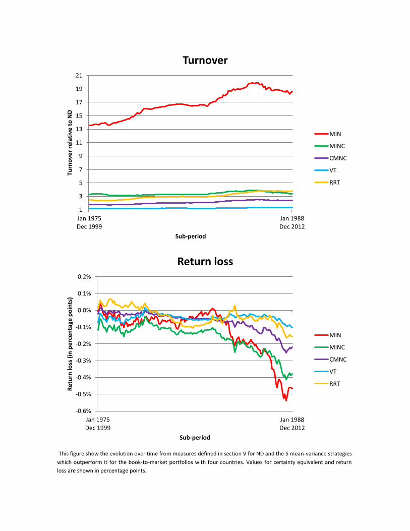
This figure show the evolution over time from measures defined in section V for ND and the 5 mean-variance strategies

which outperform it for the book-to-market portfolios with four countries. Values for certainty equivalent and return

loss are shown in percentage points.

1

3

5

7

9

11

13

15

17

19

21

Jan 1975Dec 1999

Jan 1988Dec 2012

Turn

ove

r re

lati

ve t

o N

D

Sub-period

Turnover

MIN

MINC

CMNC

VT

RRT

-0.6%

-0.5%

-0.4%

-0.3%

-0.2%

-0.1%

0.0%

0.1%

0.2%

Jan 1975Dec 1999

Jan 1988Dec 2012

Re

turn

loss

(in

pe

rce

nta

ge p

oin

ts)

Sub-period

Return loss

MIN

MINC

CMNC

VT

RRT

correlations between assets are equals to zero, this of course is not the case, in fact correlations

between portfolios are in our data positive and large, especially between the 3 portfolios of each

country, but the reduction in parameters estimated outperform the losses due to specification

error and these strategies increase naïve diversification in Sharpe ratio criteria over time, these

improvement can supposed up to a 20%, showing again that simplicity can lead to better results.

For the first third of sub-periods VT outperforms RRT while the opposite occurs during the

remaining, but the differences between both are always small.

Bigger turnover correspond to MIN as already appointed, not allowing short-selling or combining

with naïve diversification reduces it, as shown by MINC or CMIN turnovers. VT is clearly the

strategy, apart from naïve diversification with a lesser and most stable turnover that is due to all

the restrictions implied in this strategy, therefore portfolio weights only change as a result of

movements in the assets relative variances, as seen in equation (11), which are more stable than

for example expected returns, especially, as in this case, where every risky asset we consider is in

fact a portfolio of assets, leading to even more stable variances. RRT which is like VT but also

consider changes in portfolio weights based on movements of expected returns, generates three

times the turnover of VT, more importantly in the last sub-periods when financial crisis is included

as a consequence of more changing expected returns.

Return loss show the most variable results among strategies. In general, these optimization

strategies outperform naïve diversification but this increased performance depends greatly on the

data. In general, MINC performs the best. It outperforms ND through all the series, especially since

the start of the financial crisis. MIN is in general the second best strategy, although it ranges from

first to last position depending on the sub-period analyzed. As all already stated, it performs better

when stocks markets are in crisis, that special true in the current financial crisis when allowing

short selling compensate for the increase in turnover. CMNC performs worse than MINC despite

having a lesser turnover, and except for the latest sub-periods it presents more stable results, so

combining with ND tends to reduce variance in return loss. But, the more stable strategy is VT, its

results are the least affected by different sub-periods, as a consequence of being the less

aggressive strategy with a turnover similar to that of naïve diversification.

So, at least for the best strategies according to return loss, financial crisis has augmented the

benefits of active portfolio optimization. Although, it is important to keep in mind that the sub-

periods studied lasts for 300 months, so at most, financial crisis represents a 20% of the total

months of any sub-period.

So as conclusion, we have shown the importance of data in strategies’ performance, but despite

these changes in their measures among different sub-periods, the fact that these movements are

similar in all of them makes that the order in performance is maintain for all the sub-periods and

therefore recommendations for an investor are not affected by such variations.

VII.B. Strategies outperformed by naïve diversification in BM4

Now we study the performance over time of the strategies that do not outperform naïve

diversification for the whole period (TP, CMV, TPC, KZ and JR), as shown in Figure 3. First, contrary

to the previous analysis, here there are differences between the results on Sharpe ratio and

certainty equivalent, TP has more extreme results in certainty equivalent, worse in the first sub-

periods, better in the last. Second, variations in Sharpe ratio and certainty equivalent through time

are as big as before, especially in certainty equivalent where TP strategy varies from -1.2% in the

sub-period April 1975 – March 2000, to 0.6% only one month later, that is, with 299 of 300 months

being the same in both sub-periods. Third, variations in Sharpe ratio and certainty equivalent are

different over time, as sub-periods includes more recent data, more strategies outperform naïve

diversification, more evident in Sharpe ratio where ND starts as beating these strategies, and ends

being outperformed by all of them. So strategies recommendations based on these measures are

greatly affected by the data used. Fourth, turnover values of TP, KZ and JR for the first sub-periods

are enormous compared to the remaining sub-periods, TP starts with a turnover more than 600

times that of naïve diversification and seven months later is only 100 times that of ND. Moreover,

bigger turnover results in worse performance, so aggressive strategies do not tend to improve

performance. And fifth, results on return loss again are dependent of the dates used. For most of

the sub-periods, these strategies are outperformed by ND, but for more recent dates some of

them improve naïve diversification. For example, KZ has a return loss of nearly 2.5% in the January

1975 – December 1999 sub-period but it has a -0.4 when the dates considered range from August

1987 – July 2012 where is only outperformed by three strategies, and therefore outperforms

strategies that analyzing the whole period have been considered better.

Looking for more specific results, we start with Sharpe ratio and certainty equivalent analysis. TP

strategy follows Markowitz’s methodology, which do not account for estimation errors. This

strategy is optimal when moments of returns are known, but this is not the case when are

unknown due to estimation errors. Focusing on certainty equivalent, as we are optimizing

investor’s utility, TP not only is not optimal in the first sub-periods, is in fact the worst in

performance, while for the last sub-periods outperforms all the strategies, even MIN. This erratic

behavior comes as a result on the way we are estimating the moments of returns. We assume

them to be the mean of the returns of the previous ten years, when this happens, TP is in fact

optimal, but this is not always the case and can lead to very poor performance. Nevertheless, if we

account for transaction costs even when it performs better is unable to beat naïve diversification

due to its high turnover, so measures that deal with estimation errors and reduce turnover are

always necessary.

Bayesian strategy JR is in practice very similar to TP as portfolio weights are calculated with the

same formula but with different estimates of expected returns and variances. Its Sharpe ratio’s

performance has the same exact evolution as TP but with higher values, so is an improvement

over TP, but this increase is not always enough to beat ND. This situation continues in certainty

equivalent for most of the sub-periods, and as JR reduces turnover it leads to better return loss

than TP in every occasion, but again not enough to beat ND apart from some recent sub-periods.

Figure 3: Evolution over time out-of-sample of outperformed strategies by ND in BM4

0

0.05

0.1

0.15

0.2

0.25

0.3

Jan 1975Dec 1999

Jan 1988Dec 2012

Shar

pe

rat

io

Sub-period

Sharpe ratio

ND

TP

CMV

TPC

KZ

JR

-1.5%

-1.0%

-0.5%

0.0%

0.5%

1.0%

1.5%

2.0%

Jan 1975Dec 1999

Jan 1988Dec 2012

ceq

(in

pe

rce

nta

ge p

oin

ts)

Sub-period

Certainty equivalent

ND

TP

CMV

TPC

KZ

JR

This figure show the evolution over time from measures defined in section V for ND and the 5 mean-variance

strategies which are outperformed by it for the book-to-market portfolios with four countries. Values for certainty

equivalent and return loss are shown in percentage points, and turnover is shown in logarithmic scale.

1

10

100

1000

Jan 1975Dec 1999

Jan 1988Dec 2012

Turn

ove

r re

lati

ve t

o N

D (

loga

ritm

ic s

cale

)

Sub-period

Turnover

TP

CMV

TPC

KZ

JR

-1.0%

-0.5%

0.0%

0.5%

1.0%

1.5%

2.0%

2.5%

3.0%

Jan 1975Dec 1999

Jan 1988Dec 2012

Re

turn

loss

(in

pe

rce

nta

ge p

oin

ts)

Sub-period

Return loss

TP

CMV

TPC

KZ

JR

Because MIN strategy performs better than ND in Sharpe ratio and certainty equivalent, not

surprisingly KZ outperforms CMV in general. As already stated, combinations tend to achieve in

these measures an average between its components. In turnover, both strategies have similar

values, except in the initials periods, when as the TP turnover of KZ its more than the double of its

mean, which of course affects its return loss, but apart from these initials periods, KZ outperforms

CMV and even ND in recent dates, although MIN still beats it.

Finally, restraining short selling to TP leads to an improvement except for the last sub-periods,

because for them short selling is quite important, something already notice in the difference

between MIN and MINC in these dates. But due to the reduction of turnover consequence of this

limitation when looking for its return loss, its results improve the unrestricted TP.

As a conclusion, it is evident that results from different strategies depend on the data from which

optimization is calculated. If estimation errors are small as a consequence of parameters

estimated being similar to real ones, then Markowitz’s rule performs the best as is closer to the

optimal and modifications adopted to deal with estimation error worsens performance as not

enough estimation error is reduced to compensated errors in specification. But, this not occurs in

general, from the 156 sub-periods analyzed here, TP has the higher certainty equivalent only for

the last 12 sub-periods. In fact, this also occurs for the other strategies that include or are similar

to TP, such as JR, KZ or CMV, that in general are outperformed by ND and most of the strategies,

except for the most recent sub-periods, showing the trade-off between estimation error and

specification error. Even more, when transactions costs are added, TP is never optimal so methods

that reduce estimation error and turnover are always necessary, and the results obtained for the

whole period are still maintained.

VII.C. Robustness of outperformers of naïve diversification

In this section, we concentrate in analyze if the strategies that would be recommended to an

investor if we consider the whole data period, would be also the optimal choice for different sub-

periods. To do this, we comment the performance over time for the best strategies on return loss,

as is more realistic to consider transaction costs, when we consider book-to-market portfolios,

except when the number of countries is four as this has been already explained in the two

previous sections.

When only Spain and Italy are used to form portfolios, MINC, MIN and RRT are respectively the

three strategies with better return loss for the whole period. When we look for different sub-

periods, three different strategies MINC, TPC and RRT are the best choice for different sub-periods

but they also have sub-periods when they can’t outperform naïve diversification, while MINC has

more stable results an always outperforms ND.

If we allows portfolios to be formed with assets from six different countries, therefore ,

MINC is clearly the best return loss with CMNC and CMIN following it. Not surprisingly, MINC is still

the optimal choice for almost all the sub-periods. While MIN which is the fourth better strategy,

and although beats ND for the whole period, when we look on their evolution over time is

outperformed by ND when we account for transaction costs in most of the sub-periods and only in

recent dates improves ND on return loss, showing a result less favorable than that of only one

result considered.

As Norway and Sweden portfolios are added to the previous ones, the outperformers are quite

similar, with again MINC achieving the lead in return loss for the one period, and also for almost all

the sub-periods. Thus, MINC recommendation is robust over time.

Finally, when all ten countries period can be used to optimize portfolios only three strategies beat

ND for the whole MINC, VT and CMNC, as a result of the increased number of parameters which

need estimation. Contrary to the other cases, here in the more recent periods is when ND

dominates all the strategies, and none outperforms ND by more than a 0.2% in any sub-period.

From all these results, we can conclude that caution must be taken when recommending a

strategy based solely in the performance results of the whole period, as strategies’ performance

can greatly change among different sub-periods.

VIII. Conclusion

Markowitz (1952) defined a framework to optimally maximize investor’s utility by allocating risky

assets, but errors in the estimation of moments needed and its aggressiveness, resulting in

extreme portfolio weights, leads to bad results out-of-sample, therefore is empirical usefulness for

investors is limited.

Following DeMiguel, Garlappi and Uppal (2009) we have compared the performance of 14

different mean-variance strategies, but our contribution has been to include recent proposals not

hugely studied, in 10 European capital markets, where most of the literature has concentrate in

the US market. Contrary to DeMiguel, Garlappi and Uppal (2009), who did not obtain any strategy

outperform naïve diversification in all their data from the US markets, when we consider the

whole period we have proved that active portfolio management can beat naïve diversification for

all the European datasets considered, especially when the number of assets is small, because as

we consider assets of new countries, more parameters have to be estimated and errors limit the

benefits of portfolio optimization. Particularly minimum variance, a less aggressive strategy which

targets a low return, obtains the best results in Sharpe ratio and certainty equivalent due to its

reduced estimation errors by only consider variance-covariance matrix to determine portfolio

weights. When we consider transaction cost, MIN is no longer the best strategy for an investor to

follow due to an important turnover. Other strategies that needs lesser changes in portfolio

weights beat MIN and ND, although their inferior Sharpe ratios and certainty equivalents. This

group of outperformers is formed, in order of better return loss and hence in order of preference

of an investor, by minimum variance without short selling, an optimal combination of naïve and

minimum variance without short selling strategy and volatility timing. All of these three strategies

have in common the use of various restrictions and simplifications over mean-variance framework

that approximate them to the benefits of naïve diversification, Kirby and Ostdiek (2012) define

precisely VT to achieve this goal. As ND all of them do not short sell, do not estimated expected

returns and have low turnover, therefore design strategies that share these restriction could also

obtain adequate performance.

A great number of the strategies considered consist of strategies that combine naïve

diversification with other strategies. We have confirmed the results obtained by Tu and Zhou

(2011), and these combinations improve the performance of strategies that individually perform

worse than ND, but when we calculate combinations with strategies that beat ND this leads to

worsen performance. Hence, combining with ND leads to strategies with performance

intermediate between its components.

We analyzed the performance of the strategies in different sub-periods. We have observed that

changes between sub-periods that only change by two dates suffer enormous variations but the

order of preference does not change in the strategies that achieve the highest performances.

Therefore, although caution must be taken when all the information related to the performance is

reduced to a single number, in our case the results from the whole period are robust and

recommendations of investor’s strategy maintain.

References

Avramov, D. 2002. Stock Return Predictability and Model Uncertainty. Journal of Financial

Economics 64:423-58.

Bawa, V. S., Brown, S., Klein, R. W. 1979. Estimation Risk and Optimal Portfolio Choice. Amsterdam,

The Netherlands: North Holland.

Black, F., Litterman, R. 1992. Global Portfolio Optimization. Financial Analysts Journal 48:28-43.

Brandt, M. W. 2010. Portfolio Choice Problems, in Y. Ait-Sahalia and L. P. Hansen (eds.), Handbook

of Financial Econometrics.

Brown, S. 1979. The Effect of Estimation Risk on Capital Market Equilibrium. Journal of Financial

and Quantitative Analysis 14:215-20.

Chapados, N. 2011. Portfolio Choice Problems: An Introductory Survey of Single and Multiperiod

Models in SpringerBriefs in Electrical and Computer Engineering Volume 3.

Chopra, V. K., Ziemba, W. T. 1993. The Effects of Errors in Means, Variances and Covariances on

Optimal Portfolio Choice. Journal of Portfolio Management 19:6-11.

DeMiguel, V., Garlappi, L., Uppal, R. 2009. Optimal Versus Naïve Diversification: How Inefficient is

the 1/N Portfolio Strategy. Review of Financial Studies 22:1915-53.

Frankfurter, G. M., Phillips, H. E., Seagle, J. P. 1971. Portfolio selection: The Effects of Uncertain

Means, Variances and Covariances. Journal of Financial and Quantitative Analysis 6:1251-1262.

Frost, P. A., Savarino, J. E. 1986. An Empirical Bayes Approach to Efficient Portfolio Selection.

Journal of Financial and Quantitative Analysis 21:293-305.

Frost, P. A., Savarino, J. E. 1988. For Better Performance Constrain Portfolio Weights. Journal of

Portfolio Management 15:29-34.

Goldfarb, D., Iyengar, G. 2003. Robust Portfolio Selection Problems. Mathematics of Operations

Research 28:1-38.

Jagannathan, R., Ma, T. 2003. Risk Reduction in Large Portfolios: Why Imposing the Wrong

Constraints Helps. Journal of Finance 58:1651-84.

James, W., Stein, C. 1961. Estimation with Quadratic Loss. Proceedings of the forth Berkeley

Symposium on Probability and Statistics I. Berkeley, CA: University of California Press.

Jobson, J. D., Korkie, R., Ratti, V. 1979. Improved Estimation for Markowitz Portfolios Using James-

Stein Type Estimators. Proceedings of the American Statistical Association 41:279-92.

Jorion, P. 1986. Bayes-Stein Estimation for Portfolio Analysis. Journal of Financial and Quantitative

Analysis 21:279-92.

Kan, R., Zhou, G. 2007. Optimal Portfolio Choice with Parameter Uncertainty. Journal of Financial

and Quantitative Analysis 42:621-56.

Kirby, C., Ostdiek, B. 2012. It’s All in the Timing: Simple Active Portfolio Strategies that Outperform

Naïve Diversification. Journal of Financial and Quantitative Analysis 47:437-67.

Klein, R. W., Bawa, V. S. 1976. The Effect of Estimation Risk on Optimal Portfolio Choice. Journal of

Financial Economics 3:215-31.

Ledoit, O., Wolf, M. 2004. Honey, I Shrunk the Sample Covariance Matrix: Problems in Mean-

Variance Optimization. Journal of Portfolio Management 30:110-19.

Lozano, M. 2013. Asset Allocation in the Presence of Estimation Error. A Prediction-Based-Asset-

Pricing Approach. Working Paper.

MacKinlay, A.C., Pastor, L. 2000. Asset Pricing Models: Implications for Expected Return and

Portfolio Selection. The Review of Financial Studies 13:883-916.

Markowitz, H. M. 1952. Portfolio Selection. Journal of Finance 7:77-91.

Michaud, R. O. 1989. The Markowitz Optimization Enigma: Is Optimized Optimal? Financial

Analysts Journal 45:31-42.

Pástor, L. 2000. Portfolio Selection and Asset Pricing Models. Journal of Finance 55:179-223.

Pástor, L., Stambaugh, R. F. 2000. Comparing Asset Pricing Models: An Investment Perspective.

Journal of Financial Economics 56:335-81.

Stein, C. 1956. Inadmissibility of the Usual Estimator for the Mean of a Multivariate Normal

Distribution. Proceedings of the Third Berkeley Symposium on Mathematical Statistics and

Probability I(1956):197:206.

Tu, J., Zhou, G. 2004. Data-Generating Process Uncertainty: What Difference Does It Make in

Portfolio Decisions? Journal of Financial Economics 72:385-421.

Tu, J., Zhou, G. 2011. Markowitz Meets Talmud: A combination of Sophisticated and Naïve

Diversification Strategies. Journal of Financial Economics 99:204-15.

Zellner, A., Chetty, V. K. 1965. Prediction and Decision Problems in Regression Models from the

Bayesian Point of View. Journal of the American Statistical Association 60:608-16.