Out-of-Sample Equity Premium Prediction:Economic Fundamentals vs. Moving-Average Rules

Christopher J. NeelyFederal Reserve Bank of

St. Louisneely@stls.frb.org

David E. RapachSaint Louis Universityrapachde@slu.edu

Jun TuSingapore Management

Universitytujun@smu.edu.sg

Guofu Zhou∗Washington University in

St. Louis and CAFRzhou@wustl.edu

February 25, 2010

∗Corresponding author. This project was undertaken while Rapach and Zhou were Visiting Scholars at the FederalReserve Bank of St. Louis. The views expressed in this paper are those of the authors and do not reflect those of theFederal Reserve Bank of St. Louis or the Federal Reserve System.

Out-of-Sample Equity Premium Prediction:Economic Fundamentals vs. Moving-Average Rules

Abstract

This paper analyzes the ability of both economic variables and moving-average rules toforecast the monthly U.S. equity premium using out-of-sample tests for 1960–2008. Bothapproaches provide statistically and economically significant out-of-sample forecasting gains,which are concentrated in U.S. business-cycle recessions. Nevertheless, economic variablesand moving-average rules capture different sources of equity premium fluctuations: moving-average rules detect the decline in the average equity premium early in recessions, while eco-nomic variables more readily pick up the rise in the average equity premium later in reces-sions. When we simulate data with a habit-formation model characterized by time-varying re-turn volatility and risk aversion relating to business-cycle fluctuations, we find that this modelcannot fully account for the out-of-sample forecasting gains in the actual data evidenced byeconomic variables and moving-average rules.

JEL classifications: C22, C53, E32, G11, G12, G17

Keywords: Equity premium predictability; Economic variables; Moving-average rules; Out-of-sample forecasts; Asset allocation; Mean-variance investor; Business cycle; Habit forma-tion

Out-of-Sample Equity Premium Prediction:Economic Fundamentals vs. Moving-Average Rules

1. Introduction

Researchers have long investigated two very different methods of predicting aggregate stock

returns: fundamental analysis and technical analysis. Fundamental analysis uses valuation ratios,

interest rates, interest rate spreads, and related economic variables to forecast excess stock returns

or, equivalently, the equity premium. In contrast, technical analysis studies past stock price behav-

ior to ascertain future price movements and thereby guide trading decisions.

Economic fundamentals are commonly analyzed using a predictive regression framework, in

which the equity premium is regressed on a lagged potential predictor. Rozeff (1984), Fama and

French (1988), and Campbell and Shiller (1988a, 1988b) employ this framework and present evi-

dence that valuation ratios, such as the dividend yield, predict the equity premium. Similarly, Keim

and Stambaugh (1986), Campbell (1987), Breen, Glosten and Jagannathan (1989), and Fama and

French (1989) find that nominal interest rates and interest rate spreads, such as the default and

term spreads, predict the equity premium, while Nelson (1976) and Fama and Schwert (1977)

find predictive ability for the inflation rate. More recent studies continue to support equity pre-

mium predictability using valuation ratios (Cochrane, 2008; Pastor and Stambaugh, 2009), in-

terest rates (Ang and Bekaert, 2007), and inflation (Campbell and Vuolteenaho, 2004). Other

studies identify additional economic variables with predictive power, including corporate issuing

activity (Baker and Wurgler, 2000; Boudoukh, Michaely, Richardson, and Roberts, 2007), the

consumption-wealth ratio (Lettau and Ludvigson, 2001), and volatility (Guo, 2006).1

While the consensus appears to be that economic variables predict a significant component of

the U.S. equity premium (Campbell, 2000), this vast literature relies predominantly on in-sample

tests. Goyal and Welch (2008) recently argue strongly that economic fundamentals fail to consis-

tently predict the equity premium in out-of-sample tests. Given the widespread view that out-of-

sample tests are more demanding than in-sample tests, this failure casts doubt on the robustness

of return predictability and limits its usefulness to investors in real time. In response, Campbell

and Thompson (2008) show that imposing reasonable restrictions on equity premium forecasts

1This is not meant to be an exhaustive list of studies; see, for example, Campbell (2000), Cochrane (2007), Goyaland Welch (2008), and Lettau and Ludvigson (2009) for surveys of the extensive literature on return predictabilityusing economic variables.

1

improves the out-of-sample performance of a number of individual predictive regression models.

Furthermore, Rapach, Strauss, and Zhou (2010a) find that combining individual predictive re-

gression forecasts generates consistent out-of-sample gains, despite the inconsistent performance

of individual forecasts. In addition to the conventional mean squared prediction error (MSPE)

statistical metric, Campbell and Thompson (2008) and Rapach, Strauss, and Zhou (2010a) find

substantial economic value for predictability in an asset-allocation problem. Overall, there appears

to be significant out-of-sample evidence for return predictability using economic variables, at least

when individual forecasts are restricted and/or used in combination.

Technical analysis dates at least to 1700 and was popularized in the late nineteenth and early

twentieth centuries by the “Dow Theory” of Charles Dow and William Peter Hamilton.2 Despite

its popularity, academic economists have traditionally been quite skeptical of the value of tech-

nical analysis (e.g., Malkiel, 2007), because its success would violate the intuitively attractive

weak-form efficient market hypothesis, which holds that past prices—which are clearly known to

traders—should not help traders earn abnormal risk-adjusted returns.

Numerous studies examine the profitability of technical trading rules in equity markets. Early

studies, including Cowles (1933), Fama and Blume (1966), and Jensen and Benington (1970), re-

port largely negative results for a variety of popular technical indicators. Beginning in the 1990s,

however, several papers claimed success for technical analysis in the U.S. equity market, rekindling

interest in the subject. For example, Brock, Lakonishok, and LeBaron (1992) find that moving-

average and trading-range-break rules have predictive power for the Dow Jones index for 1897–

1986. Brown, Goetzmann, and Kumar (1998) reconsider the technical-based timing advice of the

Dow Theory from William Peter Hamilton’s editorials—previously examined by Cowles (1933)—

and find that it yields high Sharpe ratios and positive risk-adjusted excess returns. Furthermore,

Lo, Mamaysky, and Wang (2000) find that several technical indicators based on automatic pattern

recognition with kernel regressions have some practical value. Savin, Weller, and Zvingelis (2007)

modify Lo, Mamaysky, and Wang’s (2000) pattern recognition procedures and detect value for

“head-and-shoulders” price patterns. These positive findings are tempered by other recent stud-

ies, however. Using White’s (2000) “reality check” bootstrap, Sullivan, Timmermann, and White

(1999) confirm the results for 1897–1986 in Brock, Lakonishok, and LeBaron (1992), but they find

little support for the profitability of trading rules for 1987–1996. Allen and Karjalainen (1999) ap-

2Nison (1991) notes that Munehisa Homma reportedly made a fortune in eighteenth-century Japan using an earlyversion of “candlestick” patterns to predict rice market prices using past prices. Schwager (1993, 1995) and Covel(2005) discuss how technical analysis is an important tool for many of today’s most successful traders.

2

ply genetic programming—an automated procedure to search for ex ante “optimal” trading rules—

to S&P 500 data for 1928–1995 but fail to identify rules that outperform a simple buy-and-hold

strategy. Neely (2003) confirms Allen and Karjalainen’s (1999) results for risk-adjusted excess

returns. In summary, a number of studies present evidence that technical indicators provide infor-

mative trading signals, although the performance of various indicators can vary over time.3

The literatures on return predictability based on economic fundamentals and technical analysis

have evolved largely independently of each other. Since both literatures report evidence of return

predictability, this raises a number of intriguing questions: Does one approach clearly outperform

the other? Do economic fundamentals and technical indicators capture similar return predictabil-

ity patterns in the data? To what extent is the predictive power of each approach related to the

real economy and business-cycle fluctuations? Should fundamental and technical approaches be

viewed as substitutes or complements in asset-allocation decisions? In the present paper, we merge

the two literatures in an attempt to answer these important questions. We do this by comparing the

out-of-sample predictive ability of a host of popular economic fundamentals to that of a num-

ber of moving-average (MA) rules. MA rules are relatively transparent technical indicators that

conveniently embody the trend investigation at the heart of technical analysis.

Our strategy for merging the two literatures has four key elements. First, we compare equity

premium forecasts based on economic fundamentals and MA rules in terms of the Campbell and

Thompson (2008) out-of-sample R2 statistic, which measures the reduction in MSPE for a com-

peting forecasting model relative to the historical average (random walk with drift) benchmark

forecast. Goyal and Welch (2008) show that the historical average forecast is a very stringent

benchmark. Following Campbell and Thompson (2008) and Goyal and Welch (2008), we generate

equity premium forecasts based on economic fundamentals using recursively estimated predictive

regression models. While MA rules provide trading signals—rather than point forecasts per se—

we transform the signals into point forecasts using a recursive regression framework. This allows

us to directly compare equity premium forecasts based on economic variables and MA rules.

Second, we compare the economic value of equity premium forecasts based on either set of

variables from an asset-allocation perspective. More specifically, we calculate utility gains in a

simulated real-time setting for a mean-variance investor who optimally allocates a portfolio be-

tween equities and a risk-free Treasury bill using equity premium forecasts based on either eco-

3Again, this is not meant to be an exhaustive list of studies; see Park and Irwin (2007) for a survey of the technicalanalysis literature for the equity and foreign exchange markets. Menkhoff and Taylor (2007) provide an extensivesurvey focusing on technical analysis in the foreign exchange market.

3

nomic variables or MA rules relative to an investor who uses the historical average equity premium

forecast. While numerous studies investigate the profitability of technical indicators, these studies

are ad hoc in the sense that the degree of risk aversion is not incorporated into the asset-allocation

decision. Analogous to Zhu and Zhou (2009), we address this drawback in a utility framework by

generating point forecasts based on MA rules that can be used for optimal portfolio allocation by

a mean-variance investor. We compare the utility gains for a risk-averse investor who forecasts the

equity premium using economic variables to the utility gains for an investor with the same degree

of risk aversion who forecasts the equity premium with MA rules.

Third, to explore links between out-of-sample return predictability and the real economy, we

compute out-of-sample R2 statistics and utility gains for equity premium forecasts based on eco-

nomic fundamentals and MA rules during both expansions and recessions, and we examine closely

the behavior of the forecasts over the course of recessions. Insofar as predictability is linked to the

real economy, we expect that there will be more predictability in the rapidly changing macroeco-

nomic conditions of recessions, as evidenced by Henkel, Martin, and Nadari (2009) and Rapach,

Strauss, and Zhou (2010b), who show that equity premium predictability using economic variables

is concentrated in cyclical downturns.

In our comparison study, we find that monthly equity premium forecasts based on both eco-

nomic fundamentals and MA rules often outperform the historical average benchmark forecast

according to the out-of-sample R2 and utility metrics, but that the gains are concentrated during

business-cycle recessions. For example, a mean-variance investor with a risk aversion coefficient

of five would pay an annualized portfolio management fee of 1.82% to have access to the equity

premium forecast based on the dividend yield relative to the historical average benchmark forecast

for the entire 1960:01–2008:12 forecast evaluation period; during recessions, the same investor

would pay a hefty 13.02%. Similarly, an investor with the same preferences would pay a fee of

3.43% during the full forecast evaluation period and 16.78% during recessions for access to an

equity premium forecast based on an MA(1,12) rule rather than the historical average benchmark.

Overall, our results connect equity premium predictability based on both economic fundamentals

and technical indicators to business-cycle fluctuations.

Although both economic and technical variables forecast better during recessions, the two ap-

proaches exploit different patterns. MA rules generally detect the falling average equity premium

early in recessions, while economic fundamentals correctly pick up the rising average equity pre-

mium later in recessions near business-cycle troughs. These results help to explain the simultane-

4

ously prominent roles for economic fundamentals in the academic literature and technical indica-

tors among practitioners. Both approaches seem useful for predicting returns, and they appear to

complement each other.

Our results also provide insight into the time-varying nature of the return predictability litera-

ture. Henkel, Martin, and Nadari (2009) observe that because equity premium predictability using

economic fundamentals is concentrated in recessions, empirical findings will depend on the preva-

lence of such conditions in particular studies. Early predictability studies employing economic

variables typically use samples ending in the early-to-mid 1980s. Relatively large parts of the

samples in these studies will thus include the turbulent 1970s and the deep recession of the early

1980s. Later studies, such and Goyal and Welch (2008), use samples that cover much of the “Great

Moderation” stretching from the mid 1980s to the early 21st century, which will dampen the ev-

idence of predictability emanating from economic fundamentals. Empirical studies of technical

analysis display similar time variation. For example, Brock, Lakonishok, and LeBaron (1992)

find significant evidence for the profitability of technical rules for 1897–1986, a sample covering

numerous severe recessions, including the Great Depression. While confirming their findings for

1897–1986, Sullivan, Timmermann, and White (1999) fail to find support for technical rules for

1987–1996, a sample that falls entirely within the Great Moderation and includes only a single

recession, the relatively mild 1990–1991 recession. Given that both economic fundamentals and

MA rules evince much stronger predictability during recessions, we expect that both literatures

will find stronger support for predictability when incorporating more recent data from the “Great

Recession” beginning in 2008, as our study portends.

Finally, we explore whether rational fluctuations in the expected equity risk premium can ac-

count for the out-of-sample forecasting gains demonstrated by economic variables and MA rules.

Specifically, we simulate data from the Campbell and Cochrane (1999) habit-formation model that

generates time-varying conditional return volatility and risk aversion relating to business-cycle

fluctuations. If the economic variables and technical indicators exploit only rational fluctuations

of the type produced by this model, the simulated data should show comparable forecastability to

the real data. This is not the case, however, as empirical p-values indicate that the out-of-sample

gains typically remain significantly greater than those in the simulated data.

The remainder of the paper is organized as follows. Section 2 outlines the construction of

point forecasts of the equity premium based on economic fundamentals and MA rules, as well as

the forecast evaluation criteria. Section 3 reports empirical results for the forecast comparisons.

5

Section 4 examines the ability of a habit-formation model to account for the out-of-sample results.

Section 5 contains concluding remarks.

2. Econometric Methodology

This section outlines the construction and evaluation of out-of-sample equity premium point

forecasts based on both economic variables and MA rules.

2.1. Construction of Point Forecasts

The conventional framework for analyzing return predictability based on economic variables

is the following predictive regression model:

rt+1 = αi +βixi,t + εi,t+1, (1)

where rt+1 is the return on a broad stock market index in excess of the risk-free rate from time t

to t + 1, xi,t is a predictor, and εi,t+1 is a disturbance term. To generate out-of-sample forecasts

based on (1), we first divide the total sample of T observations into m in-sample and q out-of-

sample observations, where T = m+ q. The initial out-of-sample equity premium forecast for

period m+1 using the economic variable xi,t is given by

ri,m+1 = αi,m + βi,mxi,m, (2)

where αi,m and βi,m are the ordinary least squares (OLS) estimates of αi and βi, respectively, in (1)

computed by regressing {rt}mt=2 on a constant and {xi,t}m−1

t=1 . The subsequent forecast for period

m+2 is given by

ri,m+2 = αi,m+1 + βi,m+1xi,m+1, (3)

where αi,m+1 and βi,m+1 are the OLS estimates calculated by regressing {rt}m+1t=2 on a constant and

{xi,t}mt=1. We proceed in this manner through the end of the available out-of-sample period, pro-

ducing a set of q out-of-sample equity premium forecasts based on xi,t , {ri,t+1}T−1t=m . This procedure

simulates a real-time forecasting exercise.4 Observe that the forecasts are generated using a recur-

sive (or expanding) estimation window. Forecasts could also be generated using a rolling window,4This is apart from data availability and revisions, of course. Data availability and revisions are typically not an

issue for the economic variables considered in the literature. For the monthly data that we employ in Section 3, theinflation rate is the only economic variable not available at the end of the month. Following Goyal and Welch (2008),we thus replace xi,t with xi,t−1 for the inflation rate in the predictive regression model given by (1).

6

which drops earlier observations as additional observations become available. Rolling samples are

sometimes justified by appealing to structural instability. Pesaran and Timmermann (2007) and

Clark and McCracken (2009), however, show that it can be optimal to include pre-break data when

estimating a forecasting model for a quadratic loss function, due to the familiar bias-efficiency

tradeoff.5

The historical average equity premium forecast, rt+1 = (1/t)∑tj=1 r j, is a natural benchmark

corresponding to the random walk with drift model. In their influential study, Goyal and Welch

(2008) show that rt+1 is a stringent benchmark. More specifically, they find that forecasts from

individual predictive regression models based on numerous economic variables from the literature

are unable to consistently outperform the historical average forecast.

Campbell and Thompson (2008) find that restrictions help individual predictive regression fore-

casts to more consistently outperform the historical average forecast of the equity premium. For

example, theory often indicates the expected sign of βi in (1), so that we set βi = 0 when forming a

forecast if the estimated slope coefficient does not have the expected sign. Campbell and Thomp-

son (2008) also recommend setting the equity premium forecast to zero if the predictive regression

forecast is negative, since risk considerations typically imply a positive expected equity premium.

Rapach, Strauss, and Zhou (2010a) analyze combinations of N individual predictive regression

forecasts. A combination forecast takes the form,

rc,t+1 =N

∑i=1

ωiri,t+1, (4)

where {ωi}Ni=1 are the ex ante combining weights and ∑

Ni=1 ωi = 1. Rapach, Strauss, and Zhou

(2010a) show that a simple averaging scheme (ωi = 1/N for all i) consistently outperforms the his-

torical average benchmark forecast, despite the inability of individual predictive regression fore-

casts to do so.6 In Section 3, we generate individual predictive regression forecasts with Campbell

5We use recursive estimation windows in Section 3, although we obtain similar results using rolling estimationwindows of various sizes.

6Rapach, Strauss, and Zhou (2010a) show that simple averaging is a type of shrinkage forecast that stabilizes in-dividual predictive regression forecasts and thereby helps to provide out-of-sample gains more consistently over time.Forecast combination is also used successfully by Mamaysky, Spiegel, and Zhang (2007), who find that combiningpredictions from an OLS model and the Kalman filter model of Mamaysky, Spiegel, and Zhang (2008) significantlyincreases the number of mutual funds with predictable out-of-sample alphas. Timmermann (2008) combines fore-casts from linear and nonlinear models of monthly stock returns. Another method for incorporating information fromnumerous predictors is to include them simultaneously in a multiple regression model—a general or “kitchen sink”model. Goyal and Welch (2008) and Rapach, Strauss, and Zhou (2010a) find, however, that this approach performsvery poorly in out-of-sample equity premium forecasting. This is not surprising, given the well-known result thatunrestricted, highly parameterized models often entail in-sample overfitting that translates into poor out-of-sampleforecasting performance. Ludvigson and Ng (2007) pursue an alternative strategy by incorporating information from

7

and Thompson (2008) restrictions imposed and compute a combination forecast as a simple aver-

age of the individual predictive regression forecasts.

Technical indicators, such as MA rules, generate a trading signal (e.g., buy/sell), rather than a

point forecast per se. Consider an MA rule that, in its simplest form, provides a buy or sell signal

(St+1 = 1 or St+1 = 0, respectively) by comparing two moving averages:

St+1 =

{1 if MAs,t ≥MAl,t0 if MAs,t < MAl,t

, (5)

where

MA j,t = (1/ j)j−1

∑i=0

Pt−i for j = s, l, (6)

Pt is the level of a stock price index, s (l) is the size of the short (long) MA (s < l), and St+1 = 1

(St+1 = 0) signals positive (negative) expected excess returns.

We denote the MA rule with MA sizes s and l as MA(s, l). Intuitively, the MA rule is designed

to detect changes in stock price trends. For example, when prices have been falling, the short MA

will tend to be lower than the long MA. If prices begin trending upward, then the short MA tends to

increase faster than the long MA, eventually exceeding the long MA and generating a buy signal.

To directly compare MA rules to economic variables with statistical and economic metrics, we

use MA trading signals to generate point forecasts of the equity premium in a regression frame-

work.7 Consider the following regression model:

rt = αs,l +β

s,lSs,lt + ε

s,lt , (7)

where Ss,lt is the trading signal generated by MA(s, l) based on information through period t− 1.

Analogous to the procedure for computing recursive out-of-sample forecasts based on (1), the

initial out-of-sample forecast for period m+1 based on MA(s, l) is given by

rs,lm+1 = α

s,lm + β

s,lm Ss,l

m+1, (8)

where αs,lm and β

s,lm are the OLS estimates of αs,l and β s,l , respectively, in (7) computed by regress-

ing {rt}mt=1 on a constant and {Ss,l

t }mt=1. The next forecast for period m+2 is given by

rs,lm+2 = α

s,lm+1 + β

s,lm+1Ss,l

m+2, (9)

where αs,lm+1 and β

s,lm+1 are the OLS estimates calculated by regressing {rt}m+1

t=1 on a constant and

{Ss,lt }m+1

t=1 . Proceeding through the remainder of the out-of-sample period produces q out-of-sample

equity premium forecasts based on Ss,lt , {rs,l

t+1}T−1t=m .

a very large number of macroeconomic and financial variables to predict stock returns and volatility using a dynamicfactor model.

7Gencay (1998) uses a similar approach to map daily trading signals to point forecasts of the Dow Jones index.

8

2.2. Forecast Evaluation

We consider two metrics for evaluating forecasts. The first is the Campbell and Thompson

(2008) out-of-sample R2 statistic, R2OS, which measures the proportional reduction in MSPE for a

competing model relative to the historical average forecast. It is similar to the familiar in-sample

R2 statistic and is given by

R2OS = 1− ∑

qk=1(rm+k− rm+k)

2

∑qk=1(rm+k− rm+k)2 , (10)

where rm+k represents an equity premium forecast based on an economic variable or MA rule.

Clearly, when R2OS > 0, the competing forecast outperforms the historical average benchmark in

terms of MSPE.

We employ the Clark and West (2007) MSPE-adjusted statistic to test the null hypothesis that

the competing and historical average forecasts have equal MSPE against the alternative hypoth-

esis that the competing forecast has a lower MSPE, which corresponds to H0 : R2OS = 0 against

HA : R2OS > 0. Clark and West (2007) produce the MSPE-adjusted statistic by modifying the famil-

iar Diebold and Mariano (1995) and West (1996) statistic so that it has a standard normal asymp-

totic distribution when comparing forecasts from nested models. Comparing the economic or MA

forecasts with the historical average forecast clearly entails comparing nested models, since set-

ting βi = 0 in (1) or β s,l = 0 in (7) yields the random walk with drift model.8 The MSPE-adjusted

statistic is straightforwardly calculated by first defining

ft+1 = (rt+1− rt+1)2− [(rt+1− rt+1)

2− (rt+1− rt+1)2], (11)

and then regressing { fs+1}T−1s=m on a constant. The MSPE-adjusted statistic is the t-statistic corre-

sponding to the constant, and a p-value for a one-sided (upper-tail) test is based on the standard

normal distribution. Monte Carlo simulations show that the MSPE-adjusted statistic performs well

in finite samples.

Although R2OS statistics are typically small for equity premium forecasts, since aggregate ex-

cess returns contain a large unpredictable component, a relatively small R2OS statistic can still signal

economically important gains for an investor (Kandel and Stambaugh, 1996; Xu, 2004; Campbell

and Thompson, 2008). From an asset-allocation perspective, however, the R2OS alone does not

8While the Diebold and Mariano (1995) and West (1996) statistic has a standard normal asymptotic distributionwhen comparing forecasts from non-nested models, Clark and McCracken (2001) and McCracken (2007) show that ithas a complicated non-standard distribution when comparing forecasts from nested models. The non-standard distri-bution can lead the Diebold and Mariano (1995) and West (1996) statistic to be severely undersized when comparingforecasts from nested models, thereby substantially reducing power.

9

explicitly account for the risk borne by an investor. To address this drawback, we follow Mar-

quering and Verbeek (2004), Campbell and Thompson (2008), Goyal and Welch (2008), Wachter

and Warusawitharana (2009), and Rapach, Strauss, and Zhou (2010a) and compute realized utility

gains for a mean-variance investor on a simulated real-time basis. As discussed in Section 1, this

procedure addresses the failure of many existing studies of technical trading rules to incorporate

the degree of risk aversion into the asset-allocation decision.

We consider a mean-variance investor who allocates between stocks and risk-free bills using

an equity premium forecast based on an economic variable or MA rule. At the end of period t, the

investor allocates

w j,t =1γ

r j,t+1

σ2t+1

(12)

of her portfolio to stocks during period t + 1, where γ is the coefficient of risk aversion, r j,t+1 is

an equity premium forecast formed at time t based on an economic variable or MA rule indexed

by j, and σ2t+1 is a forecast of stock return variance. Following Campbell and Thompson (2008),

we assume that the investor uses a five-year moving window of past monthly returns to estimate

the variance.9 Over the out-of-sample period, the investor who uses forecast j realizes an average

utility level of

ν j = µ j−0.5γσ2j , (13)

where µ j and σ2j are the sample mean and variance, respectively, for the portfolio formed using

the sequence of r j,t+1 forecasts. We compare (13) to the average utility for the same investor when

she instead uses the historical average, rt+1, to forecast the equity premium. At the end of period

t, she allocates

w0,t =1γ

rt+1

σ2t+1

(14)

to stocks during period t +1 and realizes an average utility of

ν0 = µ0−0.5γσ20 (15)

during the out-of-sample period, where µ0 and σ20 are the sample mean and variance, respectively,

for the portfolio formed using the sequence of historical average forecasts. The utility gain accruing

to the r j,t+1 forecast vis-a-vis the rt+1 forecast is given by the difference between (13) and (15).

We multiply this difference by 1200, so that it can be interpreted as the annual percentage portfolio

9Again following Campbell and Thompson (2008), we constrain the equity weight in the portfolio to lie between0% and 150% (inclusive), so that w j,t = 0 (w j,t = 1.5) if w j,t < 0 (w j,t > 1.5). We impose the same constraint on w0,tbelow.

10

management fee that an investor would be willing to pay to have access to the r j,t+1 forecast

relative to the historical average forecast. In Section 3, we use γ = 5; results are qualitatively

similar for other γ values.

3. Empirical Results

This section describes the data and reports the out-of-sample test results for R2OS statistics and

utility gains.

3.1. Data

Our monthly data span 1927:01–2008:12. All data are from Amit Goyal’s web page, which

provides updated data from Goyal and Welch (2008).10 The aggregate market return is the contin-

uously compounded return on the S&P 500 (including dividends), and the equity premium is the

difference between the aggregate market return and the Treasury bill rate. As in Goyal and Welch

(2008), we use the following 14 economic variables to generate predictive regression forecasts

using the recursive procedure described in Section 2.1:

• Dividend-price ratio (log), DP: difference between the log of dividends paid on the S&P 500

index and the log of stock prices (S&P 500 index), where dividends are measured using a

one-year moving sum.

• Dividend yield (log), DY: log of dividends minus the log of lagged stock prices.

• Earnings-price ratio (log), EP: log of earnings on the S&P 500 index minus the log of stock

prices, where earnings are measured using a one-year moving sum.

• Dividend-payout ratio (log), DE: log of dividends minus the log of earnings.

• Stock variance, SVAR: monthly sum of squared daily returns on the S&P 500 index.

• Book-to-market ratio, BM: ratio of book value to market value for the Dow Jones Industrial

Average.

• Net equity expansion, NTIS: ratio of twelve-month moving sums of net issues by NYSE-

listed stocks to total end-of-year market capitalization of NYSE stocks.10The data are available at http://www.bus.emory.edu/AGoyal/Research.html.

11

• Treasury bill rate, TBL: interest rate on a 3-month Treasury bill (secondary market).

• Long-term yield, LTY: long-term government bond yield.

• Long-term return, LTR: return on long-term government bonds.

• Term spread, TMS: long-term yield minus the Treasury bill rate.

• Default yield spread, DFY: BAA- minus AAA-rated corporate bond yields.

• Default return spread, DFR: long-term corporate bond return minus the long-term govern-

ment bond return.

• Inflation, INFL: calculated from the CPI (all urban consumers); we follow Goyal and Welch

(2008) and use xi,t−1 in (1) for inflation to account for the delay in CPI releases.

We use the S&P 500 index for Pt when computing the MA rule-based forecasts described in Section

2.1.11

3.2. R2OS Statistics

Panel A of Table 1 reports R2OS statistics for predictive regression forecasts based on economic

variables over the 1960:01–2008:12 forecast evaluation period. We use 1926:01–1959:12 as the

initial in-sample period when forming the recursive out-of-sample forecasts. Table 1, Panel A also

reports the R2OS for a combination of the individual predictive regression forecasts (COMBINE-

ECON) based on (4) with ωi = 1/N (N = 14). We assess the statistical significance of R2OS using

the Clark and West (2007) MSPE-adjusted statistic, as described in Section 2.2. In addition to the

full 1960:01–2008:12 forecast evaluation period, we compute R2OS statistics separately for NBER-

dated business-cycle expansions and recessions.12 The U.S. economy is in recession for 87 of the

588 months (15%) spanning 1960:01–2008:12.

According to the second column of Table 1, Panel A, nine of the 14 individual economic

variables have positive R2OS statistics, so that they outperform the historical average benchmark

forecast in terms of MSPE. Six of the nine positive R2OS statistics for the individual economic

11While daily data are frequently used to generate trading signals using technical indicators, we compute MA rulesusing monthly data to put the forecasts based on economic variables and MA rules on a more equal footing. Inongoing research, we are investigating the use of daily data to generate monthly trading signals to study the morepractical problem of maximizing portfolio performance using MA rules.

12NBER peak and trough dates that define the expansion and recession phases of the U.S. business cycle are avail-able at http://www.nber.org/cycles.html.

12

variables are significant at the 10% level or better. DP and DY have the highest R2OS statistics,

0.73% and 0.71%, respectively, among the individual economic variables. The R2OS is 0.80% for

the COMBINE-ECON forecast, which is significant at the 1% level and greater than the R2OS for

any of the individual predictive regression forecasts, similar to results reported in Rapach, Strauss,

and Zhou (2010a) for quarterly U.S. excess returns.

The last four columns of Table 1, Panel A report results separately for business-cycle expan-

sions and recessions. Recessions markedly enhance the out-of-sample predictive ability of most

economic variables compared to the historical average. For example, the predictive ability of DP

and DY—which have the largest R2OS statistics among the individual economic variables over the

full 1960:01–2008:12 forecast evaluation period—is highly concentrated in recessions: the R2OS

statistics for DP (DY) are 0.15% and 2.15% (−0.26% and 3.09%) during expansions and reces-

sions, respectively. The R2OS statistics for DP, DY, LTR, and TMS are significant at the 5% level

during recessions, despite the reduced number of available observations. The COMBINE-ECON

forecast also has an R2OS that is higher during recessions than expansions (1.01% and 0.72%, re-

spectively, both of which are significant at the 5% level). The enhanced predictive ability of eco-

nomic variables during cyclical downturns in Table 1, Panel A complements recent findings in

Henkel, Martin, and Nadari (2009) and Rapach, Strauss, and Zhou (2010b) and strongly ties out-

of-sample equity premium predictability to business-cycle fluctuations.

To learn how equity premium forecasts vary over the business cycle, Figure 1 graphs the in-

dividual predictive regression forecasts and COMBINE-ECON forecast, along with the historical

average benchmark. The vertical lines in the figure delineate NBER-dated business-cycle peaks

and troughs (in succession). Many of the individual predictive regression forecasts—especially

those that perform the best during recessions, such as DP, DY, LTR, and TMS—often increase sub-

stantially above the historical average forecast over the course of recessions, reaching distinct local

maxima near business-cycle troughs. This is particularly evident during more severe recessions,

such as the mid 1970s, the early 1980s, and the most recent recessions. While averaging across

individual forecasts produces a smoother forecast, the COMBINE-ECON forecast also exhibits

distinct spikes above the historical average forecast during severe recessions. The countercyclical

fluctuations in equity premium forecasts in Figure 1 are similar to the countercyclical fluctuations

in in-sample expected equity premium estimates reported in, for example, Fama and French (1989),

Ferson and Harvey (1991), Whitelaw (1994), Harvey (2001), and Lettau and Ludvigson (2009).

The fifth and seventh columns of Table 1, Panel A show that the average forecast value is higher

13

during recessions than expansions for a number of economic variables, especially DP and DY.

We turn next to the forecasting performance of the MA rules. Panel B of Table 1 reports R2OS

statistics for point forecasts based on MA(s, l) rules. Because the choices of s and l are somewhat

arbitrary, we consider s = 1,2 and l = 3,6,9,12,15,18,21,24, providing us with 16 individual

MA rule-based forecasts. The COMBINE-MA forecast in Panel B is a simple average of the 16

individual MA forecasts. In addition to the full 1960:01–2008:12 forecast evaluation period, we

again report results separately for NBER-dated expansions and recessions.

The second column of Table 1, Panel B shows that twelve of the 16 individual MA forecasts

have positive R2OS statistics, so that they outperform the historical average forecast according to the

MSPE metric. Seven of the twelve positive R2OS statistics are significant at conventional levels. The

R2OS is also positive for COMBINE-MA and significant at the 10% level. The MA(2,12) forecast

has the highest R2OS (1.08%) in Panel B. As seen in the fourth and sixth columns of Panel B,

the results in the second column mask important differences in predictive ability during different

phases of the business cycle. As with the economic forecasts in Panel A, the predictive ability of the

MA rules varies markedly over the business cycle: with the exception of the MA(1,24) forecast, all

of the R2OS statistics are substantially higher during recessions than expansions. The R2

OS statistics

during recessions are especially large for l values of 6–15 months, ranging from 1.45%–3.05%, all

of which are significant at the 5% level.13

Figure 2 depicts the MA forecasts, where NBER-dated peaks and troughs are again delineated

by vertical lines. Figure 2 shows that the MA forecasts often drop well below the historical average

forecast early in and throughout recessions. There are also expansionary episodes, especially for

MA forecasts based on small s values, where the MA forecasts frequently fall well below the

historical average forecast. The fourth column of Table 1, Panel B indicates that these declines

detract from the accuracy of the MA forecasts during expansions. The fifth and seventh columns of

Panel B show that the average equity premium forecast is lower during recessions than expansions

for nearly all of the MA forecasts. MA forecasts with l values of 6–15 months offer the largest

13The consideration of 32 economic and MA forecasts in Table 1 raises data-snooping concerns. The White (2000)reality check and its more powerful variant developed by Hansen (2005) are the state-of-the-art data-snooping tests.Unfortunately for our purposes, strictly speaking, the White-Hansen tests are not valid for comparing nested models.Similar to the situation analyzed by Clark and McCracken (2001) and McCracken (2007) for the Diebold and Mariano(1995) and West (1996) statistic (see footnote 8), the Hansen-White tests are potentially severely undersized whencomparing nested model forecasts. Nevertheless, to get some sense of the relevance of data snooping in Table 1, wecompute bootstrapped p-values for the Hansen (2005) SPAc and SPAu statistics to test for significant differences inMSPE relative to the historical average benchmark when considering all 32 competing forecasts. The p-values arerelatively small, 0.16 and 0.17, respectively; given that the tests are likely to be undersized, these p-values suggest thatthe results in Table 1 are not simply an artifact of data snooping.

14

accuracy gains during recessions and display the greatest differences in average forecast values

across expansions and recessions.

Overall, Table 1 and Figures 1–2 indicate that forecasts based on economic variables and MA

forecasts with moderate l values predict the U.S. equity premium out of sample, especially during

recessions. The R2OS statistics are similar in size for the best-performing economic variables and

MA rules during recessions, so that there is not strong evidence for preferring economic forecasts

over MA forecasts or vice versa according to the R2OS statistics. Table 1 and Figures 1–2, however,

point to an interesting difference in the behavior of the two types of forecasts during recessions.

Many of the forecasts based on economic variables move substantially above the historical average

forecast over the course of recessions, while MA forecasts are typically well below the historical

average forecast throughout recessions. This difference in behavior is curious, because both types

of forecasts display greater out-of-sample predictive ability during recessions. We explain this

puzzle in Section 3.4, after measuring utility gains accruing to the two types of forecasts.

3.3. Utility Gains

Table 2 reports average utility gains, in annualized percent, for a mean-variance investor with

γ = 5 who allocates across stocks and a risk-free bill using equity premium forecasts based on

economic variables (Panel A) or MA rules (Panel B) relative to the historical average benchmark

forecast. The results in Panel A indicate that forecasts based on economic variables often produce

sizable utility gains vis-a-vis the historical average benchmark. The utility gain is above 1% for six

of the individual economic variables (as well as COMBINE-ECON) in the second column, so that

the investor would be willing to pay an annual management fee of a full percentage point or more

to have access to forecasts based on economic variables relative to the historical average forecast.

Similar to Table 1, the out-of-sample gains are typically concentrated in recessions. Consider, for

example, DY, which generates the largest utility gain (1.82%) for the full 1960:01–2008:12 fore-

cast evaluation period. The utility gain is slightly negative (−0.17%) during expansions, while it

is a very substantial 13.02% during recessions. DP, TBL, LTY, LTR, TMS, and DFR also provide

utility gains above 5% during recessions. The COMBINE-ECON forecast provides more consis-

tent gains across expansions (0.97%) and recessions (1.66%), although the gains are still more

sizable during recessions.

Figure 3 portrays the equity portfolio weights computed using predictive regression, COMBINE-

ECON, and historical average forecasts. Recall that the investor uses the same volatility forecast

15

for all of the portfolio allocations, so that the equity weights only differ because of differences in

the equity premium forecast. Figure 3 shows that the equity weight computed using the historical

average forecast is procyclical. Given that the historical average forecast of the equity premium

is relatively smooth, this primarily reflects changes in expected volatility: the rolling-window es-

timate of volatility tends to be counteryclical, leading to a procyclical equity weight using (14).14

The equity weights based on economic variables often deviate substantially from the equity weight

based on the historical average, with a tendency for the weights computed using economic vari-

ables to lie below the historical average weight during expansions and to move closer to or above

the historical average weight during recessions. Panel A of Table 2 indicates that these deviations

translate into significant utility gains, especially during recessions.

Panel B of Table 2 reports average utility gains for MA forecasts relative to the historical

average benchmark. All of the utility gains are positive in the second column for the full 1960:01–

2008:12 forecast evaluation period. The MA forecasts based on l values of 12 and 15 months

have average utility gains near or above above 3%, with the MA(2,12) forecast generating the

largest gain (3.43%). Comparing the fourth and sixth columns, the utility gains are markedly

higher during recessions vis-a-vis expansions. The MA(2,12) forecast provides a leading example.

During expansions, the utility gain is only 1.07%, while it jumps to 16.78% during recessions.

The fifth and seventh columns reveal that the average equity weight is lower during recessions

than expansions for all MA forecasts. The differences between the average equity weights across

business-cycle phases are especially sizable for MA forecasts with moderate l values of 9–18

months, and these l values generate the largest gains during recessions.

Figure 4 further illustrates the tendency for equity weights computed using MA forecasts to

decrease during recessions, with equity weights based on MA forecasts typically dropping below

the weight based on the historical average forecast during cyclical downturns. Again recalling

that the investor uses the same rolling-window variance estimator for all portfolio allocations, the

declines in equity weights using MA forecasts during recessions results from declines in the MA

equity premium forecasts during recessions; see Section 3.2 and Figure 2.

In summary, Table 2 shows that equity premium forecasts based on both economic variables

and MA rules usually generate sizable utility gains, especially during recessions, highlighting the

economic significance of equity premium predictability using either approach. Comparing Panels

14French, Schwert, and Stambaugh (1987), Schwert (1989, 1990), Whitelaw (1994), Harvey (2001), Ludvigson andNg (2007), Lundblad (2007), and Lettau and Ludvigson (2009), among others, also find evidence of countercyclicalexpected volatility using alternative volatility estimators.

16

A and B of Table 2, MA forecasts typically provide larger utility gains than economic forecasts

over the full 1960:01–2008:12 forecast evaluation period and during recessions. Nevertheless,

the best-performing economic variable in Table 2, DP, generates utility gains that are reasonably

comparable to those of the best-performing MA forecasts. Table 2 also shows that MA forecasts

produce substantially lower equity weights on average during recessions relative to expansions,

while forecasts based on valuation ratios, such as DP and DY, allocate a larger portfolio share to

equity on average during recessions compared to expansions.

3.4. A Closer Look at Forecast Behavior Near Cyclical Peaks and Troughs

Tables 1–2 and Figures 1–4 present somewhat of a puzzle. For equity premium forecasts

based on both economic variables and MA rules, out-of-sample gains are typically concentrated

in business-cycle recessions. However, equity premium forecasts based on economic variables

often increase during recessions, while forecasts based on MA rules are usually substantially lower

during recessions than expansions. Despite the apparent differences in the behavior of the two

types of forecasts during recessions, the out-of-sample gains are concentrated in cyclical downturns

for both approaches. Why?

We investigate this issue by examining the behavior of the equity premium and the economic

and MA forecasts around business-cycle peaks and troughs, which define the beginnings and ends

of recessions, respectively. We first estimate the following regression model around business-cycle

peaks:

rt− rt = aP0 +

4

∑k=−2

bP0,kIP

k,t + eP0,t , (16)

where IPk,t is an indicator variable that takes a value of unity k months after an NBER-dated

business-cycle peak and zero otherwise. The estimated bP0,k coefficients measure the incremen-

tal change in the average difference between the realized equity premium and historical average

forecast k months after a cyclical peak. We then estimate a corresponding model that replaces rt

with r j,t , where r j,t signifies an economic or MA forecast of the equity premium:

r j,t− rt = aPj +

4

∑k=−2

bPj,kIP

k,t + ePj,t . (17)

The slope coefficients describe the incremental change in the average difference between an eco-

nomic or MA forecast relative to the historical average forecast k periods after a cyclical peak.

Similarly, we measure the incremental change in the average behavior of the realized equity pre-

17

mium and the economic and MA forecasts around business-cycle troughs:

rt− r = aT0 +∑

2k=−4 bT

0,kITk,t + eT

0,t , (18)

r j,t− rt = aTj +∑

2k=−4 bT

j,kITk,t + eT

j,t , (19)

where ITk,t is an indicator variable equal to unity k months after an NBER-dated business-cycle

trough and zero otherwise.

The first panel of Figure 5 graphs OLS slope coefficient estimates (in percent) and 90% confi-

dence bands for (16), and the remaining panels depict corresponding estimates for (17) based on

the economic forecasts. The first panel shows that the average equity premium moves significantly

below the historical average forecast one month before through two months after a business-cycle

peak. In other words, the equity premium declines the month before a recession begins and stays

low for three more months.

The remaining panels in Figure 5 indicate that most economic forecasts fail to pick up this

decline in the equity premium early in recessions. Only the LTR, TMS, and INFL forecasts decline

significantly on average for any of the months early in recessions when the average equity premium

itself is lower than average. The TMS forecast does the best job of matching the lower-than-average

actual equity premium for the month before through two months after a peak. However, the TMS

forecast is also significantly lower than average two months before and three and four months

after a peak, unlike the actual equity premium. The LTR forecast is significantly below average

during the two months after a peak, matching the actual equity premium, but it fails to track the

actual equity premium prior to a peak. Although the confidence bands signal a significantly lower-

than-average INFL forecast in the immediate months after a peak, the magnitude of the decline is

small. Overall, Figure 5 suggests that equity premium forecasts based on economic variables are

not particularly adept at detecting the decline in the average equity premium near cyclical peaks.

Only the LTR and TMS forecasts exhibit sizable decreases near peaks; this variation presumably

contributes to the forecasting gains for these variables in Tables 1 and 2.

How do the equity premium forecasts based on MA rules behave near cyclical peaks? The

first panel of Figure 6 again shows estimates for (16), while the other panels graph estimates for

(17) for the MA forecasts. Figure 6 reveals that MA forecasts with l values of 6–18 months move

substantially below average in the months immediately following a cyclical peak. For example, the

MA(2,12) forecast is significantly below average in the months immediately after a peak, in accord

with the behavior of the actual equity premium. Given that the actual equity premium moves below

average substantially in the month before and month of a business-cycle peak, it is not surprising

18

that the MA forecasts generally are lower than average in the first two months after a peak, since

the MA forecasts are based on signals that recognize a downward trend in equity prices. This

trend-following behavior early in recessions apparently helps to generate the sizable out-of-sample

gains during recessions for MA forecasts with moderate l values, especially MA(2,12), in Tables 1

and 2. The MA forecasts in Figure 6 tend to remain well below the historical average for too long

after a peak, however.

Figures 7 and 8 depict estimates of (18) and (19) for the economic and MA forecasts, respec-

tively. The first panel in each figure shows that the actual equity premium moves significantly

above average in the fourth through second months before a cyclical trough, so that the equity

premium is higher than usual in the late stages of recessions. Figure 7 indicates that many of the

economic forecasts, particularly those based on valuation ratios (DP, DY, EP, and BM) and LTR, are

also significantly higher than average in the fourth through second months before a trough. TMS,

DFY, and COMBINE-ECON are also significantly above average in the later stages of recessions,

although by less than the previously mentioned economic variables. The ability of many of the

economic forecasts to match the higher-than-average equity premium late in recessions helps to

account for the sizable out-of-sample gains during recessions for the economic forecasts in Tables

1 and 2.

Figure 8 shows that the MA forecasts generally start low but rise quickly late in recessions, in

contrast to the pattern in the actual equity premium. Only a few of the MA forecasts–for example,

MA(1,3), MA(1,6), and MA(1,9)–are above average in the second and third months prior to a

business-cycle trough. The out-of-sample gains for the MA forecasts during recessions in Tables

1 and 2 thus occur despite the relatively poor performance of MA forecasts late in recessions.

While the trend-following MA forecasts detect the decrease in the actual equity premium early

in recessions (see Figure 6), they are less adept at recognizing the unusually high actual equity

premium late in recessions.

Figures 5–8 paint the following nuanced picture with respect to the sizable out-of-sample gains

in Tables 1 and 2. Economic variables typically fail to detect the average decline in the actual

equity premium early in recessions, while they generally detect the average increase in the actual

equity premium late in recessions. MA rules exhibit the opposite pattern: they pick up the decline

in the actual premium early in recessions but fail to match the unusually high premium late in

recessions. Although economic and MA forecasts both generate substantial out-of-sample gains

during recessions, they capture different aspects of equity premium fluctuations during cyclical

19

downturns and thus can be viewed as complements with respect to out-of-sample equity premium

predictability. This suggests that one should rely primarily on MA (economic) forecasts near

cyclical peaks (troughs). Of course, it is notoriously difficult to forecast business-cycle turning

points in real time, making it challenging to exploit the complementarity of the economic and MA

forecasts in practice.15

4. Simulated Data From a Habit-Formation Model

We next explore whether the out-of-sample forecasting gains in Section 3 are consistent with

rational fluctuations in the expected equity premium. As emphasized by Fama (1991), this type

of exercise always involves a test of the joint null hypothesis of market efficiency and a particular

model of equilibrium expected returns. A rejection of the joint null thus does not necessarily con-

stitute evidence against market efficiency per se, since the rejection could be due to an inadequate

model of equilibrium expected returns. With this important caveat in mind, we test whether the

out-of-sample gains are consistent with the well-known Campbell and Cochrane (1999, CC) habit-

formation model. The CC model links time-varying equilibrium expected returns to business-cycle

fluctuations. This makes it a natural benchmark for our purposes, given that the out-of-sample

gains in Section 3 vary over the business cycle.16

We outline the basic structure of the CC model; see CC and Wachter (2005) for details. The

representative investor’s utility is defined over consumption, Ct , and external habit, Xt , according

to

Et

∞

∑t=0

δt (Ct−Xt)

1−γ −11− γ

, (20)

where δ > 0 (γ > 0) is the time-preference (utility-curvature) parameter. A key variable in the CC

model is surplus consumption,

St =Ct−Xt

Ct, (21)

15While beyond the scope of the present paper, which focuses on the nature of economic and MA forecasts, inongoing research we are investigating the more practical problem of improving portfolio performance by exploitingeconomic and MA forecast complementarity (also see footnote 11). More specifically, we use a model for forecastingturning points (e.g., Chauvet and Senyuz, 2009) to provide information on the extent to which we rely on economic orMA forecasts for a portfolio-allocation problem. Observe that we considered simple combinations of economic andMA forecasts. This approach, however, did not improve significantly on the economic or MA forecasts individually, sothat combining did not generate a forecast synergy in this instance. It appears that the relatively poor performance ofeconomic (MA) forecasts early (late) in recessions largely offset any gains to combining economic and MA forecastsduring recessions.

16This exercise is in the spirit of Brock, Lakonishok, and LeBaron (1992), who examine whether the profitability oftechnical strategies can be explained by GARCH processes.

20

which is related to the local curvature of the utility function (or risk aversion) via ηt = γ/St . Intu-

itively, a “small” St represents a “bad” state in which consumption is near habit. As St decreases

and ηt increases, the representative investor becomes more risk averse.

The log-level of surplus consumption obeys the following heteroskedastic, autoregressive pro-

cess:

st+1 = (1−φ)s+φst +λ (st)[∆ct+1−Et(∆ct+1)], (22)

where st = log(St), s is the unconditional mean of st , φ is the persistence parameter for st , λ (st) is

a sensitivity function, and ct = log(Ct). The sensitivity function is given by

λ (st) = (1/S)√

1−2(st− s)−1, (23)

where S = σv√

γ/(1−φ) and s = log(S).17 The log-level of consumption follows a random walk

with drift:

∆ct+1 = g+ vt+1, (24)

where vt+1 ∼ i.i.d. N(0,σ2v ).

The aggregate stock market represents a claim to the future consumption stream. The individ-

ual investor treats habit as exogenous (external habit), so that the intertemporal marginal rate of

substitution (or stochastic discount factor) is given by

Mt+1 = δ

(St+1

St

Ct+1

Ct

)−γ

. (25)

According to the first-order Euler condition,

Et(Mt+1Rt+1) = 1, (26)

where Rt+1 = (Pt+1 +Ct+1)/Pt is the gross aggregate stock market return and Pt is the stock price

(excluding dividends). In this endowment economy, Ct = Dt in equilibrium, so that Pt/Ct also

represents the price-dividend ratio, Pt/Dt .18 Using Pt/Ct = Pt/Dt and rewriting (26), we have

Et

[Mt+1

(Pt+1

Dt+1(st+1)+1

)Ct+1

Ct

]=

Pt

Dt(st), (27)

where Pt/Dt is a function of st , the only state variable for the economy. A closed-form solution

is not available for Pt/Dt ; we use the Wachter (2005) series method to numerically approximate17CC select this specification so that the risk-free real interest rate is constant. They observe that the behavior of

excess returns is not sensitive to this assumption. To ensure that (23) is positive, they also assume that st < smax, wheresmax = s+(1/2)(1− S2).

18CC also consider a model where consumption and dividends are imperfectly correlated and find that stock returnsbehave very similarly to the Ct = Dt case.

21

this pricing function.19 Observe that Pt/Dt is monotonically increasing in st . Intuitively, a lower

st value implies that consumption is closer to habit, making the representative investor more risk

averse, so that lower stock prices (higher expected returns) are required for the investor to willingly

hold risky stocks. Since st falls during recessions, the CC model generates a rising expected equity

premium near cyclical troughs.

With assumed values for δ , γ , φ , g, and σv, we can simulate consumption, dividend, stock

price, and equity premium data using the CC model. While the CC model is a general-equilibrium

model, its streamlined structure only allows us to simulate observations for two of the economic

variables considered in Section 3, DP and DY.20 Fortunately, it is these two variables that generate

the largest out-of-sample gains among the economic forecasts in Tables 1 and 2. With respect to

the MA forecasts, we focus on the MA(1,12) and MA(2,12) rules for brevity. These are two of the

best-performing MA forecasts in Tables 1 and 2.

We generate empirical p-values for the R2OS statistics and utility gains corresponding to the DP,

DY, MA(1,12), and MA(2,12) forecasts in Tables 1 and 2 via the following steps:

1. Use the CC model to generate a pseudo sample of 984 observations for consumption, divi-

dends, stock prices, and the equity premium. This pseudo sample has the same length as the

original sample (1927:01–2008:12).

2. For the pseudo sample, construct pseudo equity premium forecasts based on DP, DY, MA(1,12),

and MA(2,12) for the last 588 observations, matching the length of the forecast evaluation

period in the original sample (1960:01–2008:12).

3. Compute R2OS statistics and utility gains for the pseudo DP, DY, MA(1,12), and MA(2,12)

forecasts. In addition to computing R2OS statistics and utility gains for the full forecast evalu-

ation period of the pseudo sample, we compute these statistics for business-cycle expansions

and contractions. The random walk with drift process (24) represents the evolution of the real

economy in the CC model. It is well known that such a process can generate business-cycle-

like patterns, with peaks and troughs corresponding to similar turning points identified by the

NBER. For the simulated consumption data, we identify business-cycle peaks and troughs

that define expansions and recessions using the Harding and Pagan (2002) BB algorithm,

19Wachter (2005) finds that the series method provides a better approximation than the fixed-point method used byCC.

20Wachter (2006) extends the CC model by including multiple bonds to investigate term-structure implications ofhabit formation.

22

which provides a good approximation to the NBER business-cycle dating methodology.21

4. Repeat steps 1–3 200 times, generating empirical distributions for the R2OS statistics and util-

ity gains for the DP, DY, MA(1,12), and MA(2,12) forecasts for the full forecast evaluation

period and during expansions and recessions.

5. For each statistic, the empirical p-value is the proportion of simulated statistics greater than

the corresponding statistic in Table 1 or 2 computed using the original data.

Table 3 reproduces the R2OS statistics and utility gains from Tables 1 and 2 for the DP, DY,

MA(1,12), MA(2,12) forecasts and reports the corresponding empirical p-values (in percent) based

on the CC habit-formation model. We use the same parameter values (reported in the notes to Table

3) as those used by CC in their simulations. CC select these parameter values to match certain

moments of U.S. postwar data.

Panel A of Table 3 reports results for forecasts based on DP and DY. The empirical p-values

corresponding to the R2OS statistics for the full forecast evaluation period are above 50% for both DP

and DY. The out-of-sample predictive ability evidenced by these economic variables as measured

by R2OS is thus largely attributable to the rational fluctuations in the expected equity premium

generated by the CC model. The empirical p-values are both above 90% during expansions for

these variables. While they are substantially lower during recessions—17.5% for both DP and

DY—they are still not significant at conventional levels. Overall, the CC model appears capable of

accounting for the predictive ability of DP and DY as indicated by the R2OS statistics.

The empirical p-values for the utility gains in Table 3, Panel A point to significant gains for

DP and DY over the full forecast evaluation period (p-values of 3% and 2%, respectively) and for

DY during recessions (p-value of 7%). In interpreting these gains, keep in mind that the CC model

generates time variation in the equity premium in response to time-varying risk aversion on the

part of the representative investor. When computing utility gains, however, we consider an investor

with a constant risk aversion coefficient of five. Our non-representative investor with constant risk

aversion can thus exploit the representative investor’s time-varying risk aversion by, for example,

holding more stocks during periods when the equilibrium expected market return is elevated due

to the representative investor’s low habit and correspondingly high degree of risk aversion.22 From

21We implement the BB algorithm using James Engel’s MATLAB code downloaded fromhttp://www.ncer.edu.au/data/.

22This brings to mind a well-known Warren Buffet quote: “We simply attempt to be fearful when others are greedyand to be greedy only when others are fearful.”

23

this perspective, the significant empirical p-values in Panel A represent significant utility gains

beyond those exploitable by a non-representative investor resulting from time-varying risk aversion

on the part of the representative investor.

Empirical p-values for the MA(1,12) and MA(2,12) forecasts are reported in Table 3, Panel

B. R2OS is significant for both MA forecasts at the 1% level for the full forecast evaluation period.

The p-values for the R2OS statistics are well above 10% for both forecasts during expansions, while

R2OS is significant at the 5% and 1% levels for the MA(1,12) and MA(2,12) forecasts, respectively,

during recessions—despite the reduced number of observations. The p-values for the utility gains

in Panel B reveal significant gains at the 1% level for both forecasts for the full forecast evaluation

period and during recessions, as well as significant gains at the 5% level during expansions.

Overall, Table 3 indicates that the CC habit-formation model cannot fully account for the out-

of-sample forecasting gains offered by either the economic variables or, especially, the MA rules.

The fact that we still find significant forecasting gains according to empirical p-values generated

from the CC model, which links rational fluctuations in expected returns to business-cycle fluctu-

ations, suggests a degree of equity mispricing, perhaps relating to challenges in forecasting future

cash flows in environments, such as recessions, with rapidly changing macroeconomic fundamen-

tals. Of course, as emphasized above, the significant results in Table 3 could be due to an inad-

equate model of equilibrium expected returns. Whether alternative models that link time-varying

equilibrium expected returns to business-cycle fluctuations can explain the significant forecasting

gains evidenced by economic and MA forecasts is a fruitful area for future research.

5. Conclusion

Fundamental and technical analysis are very different methods of predicting aggregate stock

returns. While fundamental analysis relies on economic variables that are used in predictive regres-

sions, technical analysis uses functions of past price history to guide trading decisions. Researchers

have long studied both methods, but the two literatures have evolved independently; there has been

little attempt to directly compare fundamental and technical methods.

This paper fills that gap by comparing monthly, out-of-sample forecasts of the U.S. equity pre-

mium for 1960–2008 generated with well-known economic variables and popular trend-following

technical methods (i.e., MA rules). We compare the methods with two metrics: the Campbell and

Thompson (2008) out-of-sample R2 statistic and utility gains in a simulated real-time setting for

24

a mean-variance investor who optimally reallocates a monthly portfolio between equities and a

risk-free Treasury bill using equity premium forecasts.

We find evidence that both approaches produce out-of-sample forecasting gains that would be

of significant value to a mean-variance investor. While both approaches perform disproportion-

ately well during recessions, a careful analysis of their performance during cyclical downturns

reveals that they exploit very different patterns. MA rules usually recognize sooner the drop in the

average equity premium that occurs early in recessions, while economic variables tend to identify

the increase in the average equity premium prior to business-cycle troughs. Thus, fundamental and

technical approaches are complementary. This might explain the continued use of both by prac-

titioners and academics. While each approach has significant economic value, there is clearly the

possibility for dynamically combining these complementary forecasts into a superior trading rule.

Future research will investigate this issue.

We simulate data from the Campbell and Cochrane (1999) habit-formation model to study

whether this model’s rationally evolving expected equity premium can explain the forecasting

ability of economic variables and MA rules. Even though the habit-formation model connects

fluctuations in the expected equity premium to business-cycle fluctuations, simulated data from

the model cannot fully account for the forecasting gains in the actual data. Exploring whether al-

ternative models of time-varying equilibrium expected returns linked to business-cycle fluctuations

can explain these forecasting gains is yet another important area for future research.

25

References

Allen, F. and R. Karjalainen. 1999. Using Genetic Algorithms to Find Technical Trading Rules.

Journal of Financial Economics 51, 245–71.

Ang, A. and G. Bekaert. 2007. Return Predictability: Is it There? Review of Financial Studies 20,

651–707.

Baker, M. and J. Wurgler. 2000. The Equity Share in New Issues and Aggregate Stock Returns.

Journal of Finance 55, 2219–57.

Boudoukh, J., R. Michaely, M.P. Richardson, and M.R. Roberts. 2007. On the Importance of

Measuring Payout Yield: Implications for Empirical Asset Pricing. Journal of Finance 62,

877–915.

Breen, W., L.R. Glosten, and R. Jagannathan. 1989. Economic Significance of Predictable Varia-

tions in Stock Index Returns. Journal of Finance 64, 1177–89.

Brock, W., J. Lakonishok, and B. LeBaron. 1992. Simple Technical Trading Rules and the Stochas-

tic Properties of Stock Returns. Journal of Finance 47, 1731–64.

Brown, S.J., W.N. Goetzmann, and A. Kumar. 1998. William Peter Hamilton’s Track Record

Reconsidered. Journal of Finance 53, 1311–33.

Campbell, J.Y. 1987. Stock Returns and the Term Structure. Journal of Financial Economics 18,

373–99.

Campbell, J.Y. 2000. Asset Pricing at the Millennium. Journal of Finance 55, 1515–67.

Campbell, J.Y. and J.H. Cochrane. 1999. By Force of Habit: A Consumption-Based Explanation

of Aggregate Stock Market Behavior. Journal of Political Economy 107, 205–51.

Campbell, J.Y. and R.J. Shiller. 1988a. The Dividend-Price Ratio and Expectations of Future

Dividends and Discount Factors. Review of Financial Studies 1, 195–228.

Campbell, J.Y. and R.J. Shiller. 1988b. Stock Prices, Earnings, and Expected Dividends. Journal

of Finance 43, 661–676.

Campbell, J.Y. and S.B. Thompson. 2008. Predicting the Equity Premium Out of Sample: Can

Anything Beat the Historical Average? Review of Financial Studies 21, 1509–31.

Campbell, J.Y. and T. Vuolteenaho. 2004. Inflation Illusion and Stock Prices. American Economic

Review 94, 19–23.

Chauvet, M. and Z. Senyuz. 2009. A Joint Dynamic Bi-Factor Model of the Yield Curve and the

Economy as a Predictor of Business Cycles. Manuscript, University of California-Riverside.

Clark, T.E. and M.W. McCracken. 2001. Tests of Equal Forecast Accuracy and Encompassing for

26

Nested Models. Journal of Econometrics 105, 85–110.

Clark, T.E. and M.W. McCracken. 2009. Improving Forecast Accuracy by Combining Recursive

and Rolling Forecasts. International Economic Review, forthcoming.

Clark, T.E. and K.D. West. 2007. Approximately Normal Tests for Equal Predictive Accuracy in

Nested Models. Journal of Econometrics 138, 291–311.

Cochrane, J.H. 2007. Financial Markets and the Real Economy. In R. Mehra (Ed.), Handbook of

the Equity Premium. Amsterdam: Elsevier.

Cochrane, J.H. 2008. The Dog That Did Not Bark: A Defense of Return Predictability. Review of

Financial Studies 21, 1533–75.

Covel, M. 2005. Trend Following: How Great Traders Make Millions in Up or Down Markets.

New York: Prentice-Hall.

Cowles, A. 1933. Can Stock Market Forecasters Forecast? Econometrica 1, 309–24.

Diebold, F.X. and R.S. Mariano. 1995. Comparing Predictive Accuracy. Journal of Business and

Economic Statistics 13, 253–63.

Fama, E.F. 1991. Efficient Capital Markets: II. Journal of Finance 46, 1575–1617.

Fama, E.F. and M. Blume. 1966. Filter Rules and Stock Market Trading. Journal of Business 39,

226–41.

Fama, E.F. and K.R. French. 1988. Dividend Yields and Expected Stock Returns. Journal of

Financial Economics 22, 3–25.

Fama, E.F. and K.R. French. 1989. Business Conditions and Expected Returns on Stocks and

Bonds. Journal of Financial Economics 25, 23–49.

Fama, E.F. and G.W. Schwert. 1977. Asset Returns and Inflation. Journal of Financial Economics

5, 115–46.

Ferson, W.E. and C.R. Harvey. 1991. The Variation of Equity Risk Premiums. Journal of Political

Economy 99, 385–415.

French, K.R., G.W. Schwert, and R.F. Stambaugh. 1987. Expected Stock Returns and Volatility.

Journal of Financial Economics 19, 3–29.

Gencay, R. 1998. The Predictability of Security Returns with Simple Technical Trading Rules.

Journal of Empirical Finance 5, 347–59.

Goyal, A. and I. Welch. 2008. A Comprehensive Look at the Empirical Performance of Equity

Premium Prediction. Review of Financial Studies 21, 1455–508.

Guo, H. 2006. On the Out-of-Sample Predictability of Stock Market Returns. Journal of Business

27

79, 645–70.

Hansen, P.R. 2005. A Test for Superior Predictive Ability. Journal of Business and Economic

Statistics 23, 365–80.

Harding, D. and A. Pagan. 2002. Dissecting the Cycle: A Methodological Investigation. Journal

of Monetary Economics 49, 365–81.

Harvey, C.R. 2001. The Specification of Conditional Expectations. Journal of Empirical Finance

8, 573–637.

Henkel, S.J., J.S. Martin, and F. Nadari. 2009. Time-Varying Short-Horizon Predictability. Journal

of Financial Economics, forthcoming.

Jensen, M.C. and G.A. Benington. 1970. Random Walks and Technical Theories: Some Additional

Evidence. Journal of Finance 25, 469–82.

Kandel, S. and R.F. Stambaugh. 1996. On the Predictability of Stock Returns: An Asset Allocation

Perspective. Journal of Finance 51, 385–424.

Keim, D.B. and R.F. Stambaugh. 1986. Predicting Returns in the Stock and Bond Markets. Journal

of Financial Economics 17, 357–90.

Lettau, M. and S.C. Ludvigson. 2001. Consumption, Aggregate Wealth, and Expected Stock

Returns. Journal of Finance 56, 815–49.

Lettau, M. and S.C. Ludvigson. 2009. Measuring and Modeling Variation in the Risk-Return

Tradeoff. In Y. Aıt-Sahalıa and L.P. Hansen (Eds.), Handbook of Financial Econometrics.

Amsterdam: Elsevier.

Lo, A., H. Mamaysky, and J. Wang. 2000. Foundations of Technical Analysis: Computational

Algorithms, Statistical Inference, and Empirical Implementation. Journal of Finance 55,1705–

65.

Ludvigson, S.C. and S. Ng 2007. The Empirical Risk-Return Relation: A Factor Analysis Ap-

proach. Journal of Financial Economics 83, 171–222.

Lundblad, C. 2007. The Risk Return Tradeoff in the Long Run: 1836–2003. Journal of Financial

Economics 85, 123–50.

Malkiel, B.G. 2007. A Random Walk Down Wall Street: The Time-Tested Strategy for Successful

Investing. 9th Edition. New York: Norton.

Mamaysky, H., M. Spiegel, and H. Zhang. 2007. Improved Forecasting of Mutual Fund Alphas

and Betas. Review of Finance 11, 359–400.

Mamaysky, H., M. Spiegel, and H. Zhang. 2008. Estimating the Dynamics of Mutual Fund Alphas

28

and Betas. Review of Financial Studies 21, 233–64.

Marquering, W. and M. Verbeek. 2004. The Economic Value of Predicting Stock Index Returns

and Volatility. Journal of Financial and Quantitative Analysis 39, 407–29.

McCracken, M.W. 2007. Asymptotics for Out of Sample Tests of Granger Causality. Journal of

Econometrics 140, 719–52.

Menkhoff, L. and M.P. Taylor. 2007. The Obstinate Passion of Foreign Exchange Professionals:

Technical Analysis. Journal of Economic Literature 45, 936–72.

Neely, C.J. 2003. Risk-Adjusted, Ex Ante, Optimal Technical Trading Rules in Equity Markets.

International Review of Economics and Finance 12, 69–87.

Nelson, C.R. 1976. Inflation and the Rates of Return on Common Stock. Journal of Finance 31,

471–83.

Nison, S. 1991. Japanese Candlestick Charting Techniques. New York: Simon & Schuster.

Park, C.-H. and S.H. Irwin. 2007. What Do We Know About the Profitability of Technical Analy-

sis? Journal of Economic Surveys 21, 786–826.

Pastor, L. and R.F. Stambaugh. 2009. Predictive Systems: Living with Imperfect Predictors.

Journal of Finance 64, 1583–628.

Pesaran, M.H. and A. Timmermann. 2007. Selection of Estimation Window in the Presence of

Breaks. Journal of Econometrics 137, 134–61.

Rapach, D.E., J.K. Strauss, and G. Zhou. 2010a. Out-of-Sample Equity Premium Prediction:

Combination Forecasts and Links to the Real Economy. Review of Financial Studies 23, 821–

62.

Rapach, D.E., J.K. Strauss, and G. Zhou. 2010b. International Stock Return Predictability: What

is the Role of the United States? Manuscript, Washington University in St. Louis.

Rozeff, M. 1984. Dividend Yields Are Equity Risk Premiums. Journal of Portfolio Management

11, 68–75.

Savin, G., P. Weller, and J. Zvingelis. 2007. The Predictive Power of “Head and Shoulders” Price

Patterns in the U.S. Stock Market. Journal of Financial Econometrics 5, 243–65.

Schwager, J. 1993. Market Wizards: Interviews with Top Traders. New York: Harper-Collins.

Schwager, J. 1995. The New Market Wizards: Conversations with America’s Top Traders. New

York: Wiley.

Schwert, G.W. 1989. Why Does Stock Market Volatility Change Over Time? Journal of Finance

44, 1115–53.

29

Schwert, G.W. 1990. Stock Volatility and the Crash of ’87. Review of Financial Studies 3, 77–102.

Sullivan, R., A. Timmermann, and H. White. 1999. Journal of Finance 54, 1647–91.

Timmermann, A. 2008. Elusive Return Predictability. International Journal of Forecasting, 24,

1–18.

Wachter, J.A. 2005. Solving Models with External Habit. Finance Research Letters 2, 210–26.

Wachter, J.A. 2006. A Consumption-Based Model of the Term Structure of Interest Rates. Journal

of Financial Economics 79, 365–99.

Wachter, J.A. and M. Warusawitharana. 2009. Predictable Returns and Asset Allocation: Should

a Skeptical Investor Time the Market? Journal of Econometrics 148, 162–78.

West, K.D. 1996. Asymptotic Inference About Predictive Ability. Econometrica 64, 1067–84.

White, H. 2000. A Reality Check for Data Snooping. Econometrica 68, 1097–126.

Whitelaw, R.F. 1994. Time Variations and Covariations in the Expectation and Volatility of Stock

Market Returns. Journal of Finance 49, 515–41.

Xu, Y. 2004. Small Levels of Predictability and Large Economic Gains. Journal of Empirical

Finance 11, 247–75.

Zhu, Y. and G. Zhou. 2009. Technical Analysis: An Asset Allocation Perspective on the Use of

Moving Averages. Journal of Financial Economics 92, 519–44.

30

Table 1Out-of-sample equity premium forecasting results, 1960:01–2008:12 forecast evaluation period

(1) (2) (3) (4) (5) (6) (7)

Overall Expansion Recession

Average Average AveragePredictor R2

OS (%) forecast (%) R2OS (%) forecast (%) R2

OS (%) forecast (%)

A. Economic variables

DP 0.73∗∗∗ 0.25 0.15∗∗ 0.21 2.15∗∗ 0.52DY 0.71∗∗∗ 0.22 −0.26 0.17 3.09∗∗ 0.48EP −0.19 0.49 −0.15 0.44 −0.28 0.78DE −0.76 0.79 −0.80 0.80 −0.65 0.75SVAR −0.56 0.67 −0.60 0.67 −0.48 0.68BM −1.64 0.50 −1.57 0.41 −1.79 1.02NTIS −1.75 0.98 −0.34 0.96 −5.20 1.11TBL 0.31∗ 0.38 0.11∗ 0.40 0.80 0.28LTY 0.42∗∗ 0.30 0.25∗∗ 0.32 0.85 0.21LTR 0.33∗ 0.77 −0.88 0.76 3.30∗∗∗ 0.83TMS 0.14 0.81 −0.62 0.84 2.00∗∗ 0.65DFY 0.39∗ 0.64 0.33∗ 0.62 0.55 0.78DFR 0.22 0.71 0.04 0.71 0.65 0.67INFL 0.18 0.64 0.20 0.67 0.14 0.50COMBINE-ECON 0.80∗∗∗ 0.58 0.72∗∗ 0.57 1.01∗∗ 0.66

B. Moving-average rules

MA(1,3) −0.58 0.65 −1.19 0.67 0.92 0.57MA(1,6) −0.50 0.67 −1.90 0.73 2.94∗∗ 0.33MA(1,9) 0.21 0.66 −0.77 0.71 2.64∗∗ 0.37MA(1,12) 0.88∗∗ 0.68 0.19 0.74 2.57∗∗ 0.32MA(1,15) 0.82∗∗ 0.71 0.07 0.78 2.65∗∗ 0.27MA(1,18) 0.56∗ 0.69 0.01 0.76 1.91∗ 0.32MA(1,21) 0.31∗ 0.64 0.14 0.66 0.72 0.55MA(1,24) 0.06 0.62 0.11 0.61 −0.06 0.68MA(2,3) −0.17 0.65 −0.47 0.65 0.55 0.59MA(2,6) 0.21 0.66 −0.29 0.69 1.45∗∗ 0.50MA(2,9) 0.56∗ 0.66 −0.29 0.72 2.63∗∗ 0.36MA(2,12) 1.08∗∗ 0.68 0.28 0.75 3.05∗∗ 0.30MA(2,15) 0.62∗ 0.69 −0.10 0.76 2.40∗∗ 0.29MA(2,18) 0.21 0.67 −0.14 0.71 1.06 0.44MA(2,21) 0.08 0.65 −0.17 0.68 0.71 0.49MA(2,24) −0.03 0.63 −0.21 0.64 0.42 0.61COMBINE-MA 0.44∗ 0.66 −0.11 0.70 1.78∗∗ 0.44

Notes: R2OS is the Campbell and Thompson (2008) out-of-sample R2 statistic, which measures the percent reduction in mean square

prediction error for the forecast indicated in the first column relative to the historical average benchmark forecast. COMBINE-ECON(COMBINE-MA) is a combination forecast based on the individual economic-variable (moving-average) forecasts in Panel A (Panel B).Statistical significance of R2

OS is assessed with the Clark and West (2007) MSPE-adjusted statistic corresponding to the null hypothesisof equal mean square prediction error against the alternative hypothesis that the forecast indicated in the first column has a lower meansquare prediction error than the historical average benchmark forecast; ∗, ∗∗, and ∗∗∗ indicate significance at the 10%, 5%, and 1% levels,respectively. The R2

OS statistics and average forecasts are computed for the entire 1960:01–2008:12 forecast evaluation period [columns(2)–(3)] and separately for NBER-dated business-cycle expansions [columns (4)–(5)] and recessions [columns (6)–(7)]. Average forecastis the average value during the evaluation period.

Table 2Asset-allocation results, 1960:01–2008:12 forecast evaluation period

(1) (2) (3) (4) (5) (6) (7)

Overall Expansion Recession

∆ Average ∆ Average ∆ AveragePredictor (annual %) equity weight (annual %) equity weight (annual %) equity weight

A. Economic variables

DP 1.44 0.28 0.12 0.22 8.76 0.62DY 1.82 0.22 −0.17 0.17 13.02 0.55EP 1.23 0.53 0.76 0.48 3.71 0.81DE −0.53 0.98 −0.27 0.98 −1.98 0.96SVAR −0.31 0.88 −0.25 0.88 −0.66 0.88BM −0.40 0.48 −0.94 0.41 2.37 0.87NTIS −0.49 1.06 0.47 1.05 −5.97 1.12TBL 1.65 0.53 0.71 0.55 6.92 0.40LTY 1.63 0.42 0.82 0.44 6.22 0.30LTR 0.68 0.94 −0.56 0.94 7.50 0.95TMS 1.21 0.97 0.12 1.00 7.27 0.79DFY 0.43 0.82 0.20 0.80 1.61 0.96DFR 0.92 0.91 0.09 0.92 5.60 0.85INFL 0.68 0.85 0.22 0.87 3.33 0.68COMBINE-ECON 1.08 0.76 0.97 0.74 1.66 0.85

B. Moving-average rules

MA(1,3) 0.28 0.82 −0.44 0.84 4.34 0.73MA(1,6) 1.79 0.78 −0.36 0.85 13.94 0.42MA(1,9) 2.11 0.82 0.12 0.88 13.40 0.47MA(1,12) 3.07 0.84 0.96 0.92 15.03 0.39MA(1,15) 3.24 0.85 1.10 0.94 15.37 0.33MA(1,18) 2.63 0.85 0.86 0.93 12.66 0.41MA(1,21) 0.82 0.85 0.01 0.87 5.40 0.73MA(1,24) 0.05 0.82 −0.07 0.81 0.69 0.88MA(2,3) 0.35 0.84 −0.09 0.85 2.88 0.77MA(2,6) 1.02 0.85 −0.08 0.89 7.28 0.68MA(2,9) 2.35 0.83 0.32 0.89 13.88 0.47MA(2,12) 3.43 0.84 1.07 0.92 16.78 0.37MA(2,15) 2.86 0.84 0.86 0.93 14.23 0.36MA(2,18) 1.53 0.85 0.36 0.90 8.21 0.58MA(2,21) 0.94 0.85 0.09 0.89 5.79 0.66MA(2,24) 0.31 0.83 −0.13 0.84 2.81 0.80COMBINE-MA 1.78 0.85 0.45 0.90 9.35 0.58

Notes: Average utility gain (∆) is the portfolio management fee (in annualized percent return) that an investor with mean-variance preferences and riskaversion coefficient of five would be willing to pay to have access to the forecasting model given in the first column relative to the historical averagebenchmark forecasting model. COMBINE-ECON (COMBINE-MA) is a combination forecast based on the individual economic-variable (moving-average) forecasts in Panel A (Panel B). The utility gains and average equity weights are computed for the entire 1960:01–2008:12 forecast evaluationperiod [columns (2)–(3)] and separately for NBER-dated business-cycle expansions [columns (4)–(5)] and recessions [columns (6)–(7)]. Average equityweight is the average value during the evaluation period.

Table 3Empirical p-values (in percent) based on simulated data from the Campbell and Cochrane (1999) habit-formation model

(1) (2) (3) (4) (5) (6) (7)

Overall Expansion Recession

∆ ∆ ∆

Predictor R2OS (%) (annual %) R2

OS (%) (annual %) R2OS (%) (annual %)

A. Economic variables

DP 0.73 [53.50] 1.44 [3.00] 0.15 [90.50] 0.12 [58.50] 2.15 [17.50] 8.76 [12.50]DY 0.71 [59.50] 1.82 [2.00] −0.26 [94.00] −0.17 [63.00] 3.09 [17.50] 13.02 [7.00]

B. Moving-average rules

MA(1,12) 0.88 [0.50] 3.07 [0.00] 0.68 [33.50] 0.96 [3.50] 2.57 [4.00] 15.03 [0.00]MA(2,12) 1.08 [1.00] 3.43 [0.00] 0.68 [25.00] 1.07 [3.50] 3.05 [1.00] 16.78 [0.00]

Notes: The table reproduces the R2OS statistics from Table 1 and utility gains from Table 2 for equity premium forecasts based on DP, DY,

MA(1,12), and MA(2,12). Brackets report empirical p-values computed from 200 pseudo samples generated using the Campbell and Cochrane(1999) habit-formation model and the following parameter values: δ = 0.891/12, γ = 2, φ = 0.861/12, g = 0.0189/12, σv = 0.0150/

√12. The

empirical p-values are the percent of simulated R2OS statistics and utility gains greater than the corresponding reproduced values from Tables 1

and 2.

1965 1975 1985 1995 20050

0.5

1

1.5

2

DP

1965 1975 1985 1995 20050

0.5

1

1.5

2

DY

1965 1975 1985 1995 20050

0.5

1

1.5

2

EP

1965 1975 1985 1995 20050

0.5

1

1.5

2

DE

1965 1975 1985 1995 20050

0.5

1

1.5

2

SVAR

1965 1975 1985 1995 20050

0.5

1

1.5

2

BM

1965 1975 1985 1995 20050

0.5

1

1.5

2

NTIS

1965 1975 1985 1995 20050

0.5

1

1.5

2

TBL

1965 1975 1985 1995 20050

0.5

1

1.5

2

LTY

1965 1975 1985 1995 20050

0.5

1

1.5

2

LTR

1965 1975 1985 1995 20050

0.5

1

1.5

2

TMS

1965 1975 1985 1995 20050

0.5

1

1.5

2

DFY

1965 1975 1985 1995 20050

0.5

1

1.5

2

DFR

1965 1975 1985 1995 20050

0.5

1

1.5

2

INFL

1965 1975 1985 1995 20050

0.5

1

1.5

2

COMBINE−ECON

Figure 1. Out-of-sample equity premium forecasts based on economic variables, 1960:01–2008:12. Black and blue lines delineate forecasts (in percent) based onthe economic variable indicated in the panel heading and the historical average forecast, respectively. COMBINE-ECON is a combination forecast based on theindividual economic-variable forecasts. Vertical red lines show NBER-dated business-cycle peaks and troughs (in succession).

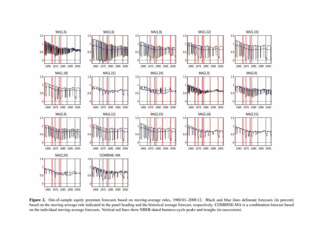
1965 1975 1985 1995 2005

0

0.5

1

1.5MA(1,3)

1965 1975 1985 1995 2005

0

0.5

1

1.5MA(1,6)

1965 1975 1985 1995 2005

0

0.5

1

1.5MA(1,9)

1965 1975 1985 1995 2005

0

0.5

1

1.5MA(1,12)

1965 1975 1985 1995 2005

0

0.5

1

1.5MA(1,15)

1965 1975 1985 1995 2005

0

0.5

1

1.5MA(1,18)

1965 1975 1985 1995 2005

0

0.5

1

1.5MA(1,21)

1965 1975 1985 1995 2005

0

0.5

1

1.5MA(1,24)

1965 1975 1985 1995 2005

0

0.5

1

1.5MA(2,3)

1965 1975 1985 1995 2005

0

0.5

1

1.5MA(2,6)

1965 1975 1985 1995 2005

0

0.5

1

1.5MA(2,9)

1965 1975 1985 1995 2005

0

0.5

1

1.5MA(2,12)

1965 1975 1985 1995 2005

0

0.5

1

1.5MA(2,15)

1965 1975 1985 1995 2005

0

0.5

1

1.5MA(2,18)

1965 1975 1985 1995 2005

0

0.5

1

1.5MA(2,21)

1965 1975 1985 1995 2005

0

0.5

1

1.5MA(2,24)

1965 1975 1985 1995 2005

0

0.5

1

1.5COMBINE−MA

Figure 2. Out-of-sample equity premium forecasts based on moving-average rules, 1960:01–2008:12. Black and blue lines delineate forecasts (in percent)based on the moving-average rule indicated in the panel heading and the historical average forecast, respectively. COMBINE-MA is a combination forecast basedon the individual moving-average forecasts. Vertical red lines show NBER-dated business-cycle peaks and troughs (in succession).

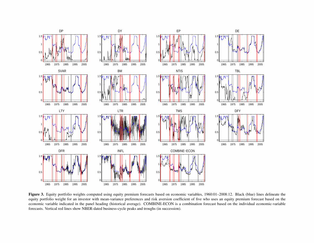
1965 1975 1985 1995 2005

0

0.5

1

1.5

DP

1965 1975 1985 1995 2005

0

0.5

1

1.5

DY

1965 1975 1985 1995 2005

0

0.5

1

1.5

EP

1965 1975 1985 1995 2005

0

0.5

1

1.5

DE

1965 1975 1985 1995 2005

0

0.5

1

1.5

SVAR

1965 1975 1985 1995 2005

0

0.5

1

1.5

BM

1965 1975 1985 1995 2005

0

0.5

1

1.5

NTIS

1965 1975 1985 1995 2005

0

0.5

1

1.5

TBL

1965 1975 1985 1995 2005

0

0.5

1

1.5

LTY

1965 1975 1985 1995 2005

0

0.5

1

1.5

LTR

1965 1975 1985 1995 2005

0

0.5

1

1.5

TMS

1965 1975 1985 1995 2005

0

0.5

1

1.5

DFY

1965 1975 1985 1995 2005

0

0.5

1

1.5

DFR

1965 1975 1985 1995 2005

0

0.5

1

1.5

INFL

1965 1975 1985 1995 2005

0

0.5

1

1.5

COMBINE−ECON

Figure 3. Equity portfolio weights computed using equity premium forecasts based on economic variables, 1960:01–2008:12. Black (blue) lines delineate theequity portfolio weight for an investor with mean-variance preferences and risk aversion coefficient of five who uses an equity premium forecast based on theeconomic variable indicated in the panel heading (historical average). COMBINE-ECON is a combination forecast based on the individual economic-variableforecasts. Vertical red lines show NBER-dated business-cycle peaks and troughs (in succession).

1965 1975 1985 1995 2005

0

0.5

1

1.5

MA(1,3)

1965 1975 1985 1995 2005

0

0.5

1

1.5

MA(1,6)

1965 1975 1985 1995 2005

0

0.5

1

1.5

MA(1,9)

1965 1975 1985 1995 2005

0

0.5

1

1.5

MA(1,12)

1965 1975 1985 1995 2005

0

0.5

1

1.5

MA(1,15)

1965 1975 1985 1995 2005

0

0.5

1

1.5

MA(1,18)

1965 1975 1985 1995 2005

0

0.5

1

1.5

MA(1,21)

1965 1975 1985 1995 2005

0

0.5

1

1.5

MA(1,24)

1965 1975 1985 1995 2005

0

0.5

1

1.5

MA(2,3)

1965 1975 1985 1995 2005

0

0.5

1

1.5

MA(2,6)

1965 1975 1985 1995 2005

0

0.5

1

1.5

MA(2,9)

1965 1975 1985 1995 2005

0

0.5

1

1.5

MA(2,12)

1965 1975 1985 1995 2005

0

0.5

1

1.5

MA(2,15)

1965 1975 1985 1995 2005

0

0.5

1

1.5

MA(2,18)

1965 1975 1985 1995 2005

0

0.5

1

1.5

MA(2,21)

1965 1975 1985 1995 2005

0

0.5

1

1.5

MA(2,24)

1965 1975 1985 1995 2005

0

0.5

1

1.5

COMBINE−MA

Figure 4. Equity portfolio weights computed using equity premium forecasts based on moving-average rules, 1960:01–2008:12. Black (blue) lines delineatethe equity portfolio weight for an investor with mean-variance preferences and risk aversion coefficient of five who uses an equity premium forecast based onthe moving-average rule indicated in the panel heading (historical average). COMBINE-MA is a combination forecast based on the individual moving-averageforecasts. Vertical red lines show NBER-dated business-cycle peaks and troughs (in succession).

−2 −1 0 1 2 3 4−6

−4

−2

0

2

4Actual

−2 −1 0 1 2 3 4

−0.6

−0.3

0

0.3

0.6

DP

−2 −1 0 1 2 3 4

−0.6

−0.3

0

0.3

0.6

DY

−2 −1 0 1 2 3 4

−0.6

−0.3

0

0.3

0.6

EP

−2 −1 0 1 2 3 4

−0.6

−0.3

0

0.3

0.6

DE

−2 −1 0 1 2 3 4

−0.6

−0.3

0

0.3

0.6

SVAR

−2 −1 0 1 2 3 4

−0.6

−0.3

0

0.3

0.6

BM

−2 −1 0 1 2 3 4

−0.6

−0.3

0

0.3

0.6

NTIS

−2 −1 0 1 2 3 4

−0.6

−0.3

0

0.3

0.6

TBL

−2 −1 0 1 2 3 4

−0.6

−0.3

0

0.3

0.6

LTY

−2 −1 0 1 2 3 4

−0.6

−0.3

0

0.3

0.6

LTR

−2 −1 0 1 2 3 4

−0.6

−0.3

0

0.3

0.6

TMS

−2 −1 0 1 2 3 4

−0.6

−0.3

0

0.3

0.6

DFY

−2 −1 0 1 2 3 4

−0.6

−0.3

0

0.3

0.6

DFR

−2 −1 0 1 2 3 4

−0.6

−0.3

0

0.3

0.6

INFL

−2 −1 0 1 2 3 4

−0.6

−0.3

0

0.3

0.6

COMBINE−ECON

Figure 5. Average actual equity premium and equity premium forecasts based on economic variables near a U.S. business-cycle peak. The panels show theincremental change in the average difference between the actual equity premium or equity premium forecast based on an economic variable and the historicalaverage equity premium forecast two months before through four months after a business-cycle peak. COMBINE-ECON is a combination forecast based on theindividual economic-variable forecasts. All forecasts are measured in percent. Circles indicate point estimates and the outer solid lines delineate 90% confidencebands.

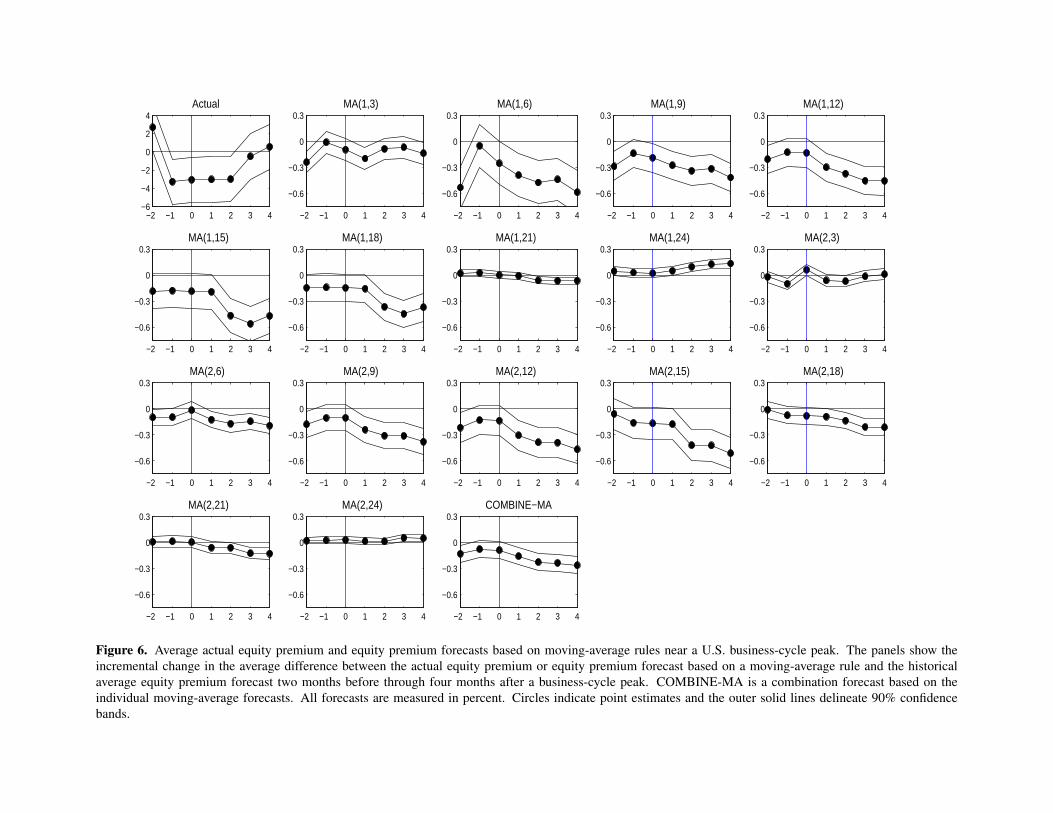
−2 −1 0 1 2 3 4−6

−4

−2

0

2

4Actual

−2 −1 0 1 2 3 4

−0.6

−0.3

0

0.3MA(1,3)

−2 −1 0 1 2 3 4

−0.6

−0.3

0

0.3MA(1,6)

−2 −1 0 1 2 3 4

−0.6

−0.3

0

0.3MA(1,9)

−2 −1 0 1 2 3 4

−0.6

−0.3

0

0.3MA(1,12)

−2 −1 0 1 2 3 4

−0.6

−0.3

0

0.3MA(1,15)

−2 −1 0 1 2 3 4

−0.6

−0.3

0

0.3MA(1,18)

−2 −1 0 1 2 3 4

−0.6

−0.3

0

0.3MA(1,21)

−2 −1 0 1 2 3 4

−0.6

−0.3

0

0.3MA(1,24)

−2 −1 0 1 2 3 4

−0.6

−0.3

0

0.3MA(2,3)

−2 −1 0 1 2 3 4

−0.6

−0.3

0

0.3MA(2,6)

−2 −1 0 1 2 3 4

−0.6

−0.3

0

0.3MA(2,9)

−2 −1 0 1 2 3 4

−0.6

−0.3

0

0.3MA(2,12)

−2 −1 0 1 2 3 4

−0.6

−0.3

0

0.3MA(2,15)

−2 −1 0 1 2 3 4

−0.6

−0.3

0

0.3MA(2,18)

−2 −1 0 1 2 3 4

−0.6

−0.3

0

0.3MA(2,21)

−2 −1 0 1 2 3 4

−0.6

−0.3

0

0.3MA(2,24)

−2 −1 0 1 2 3 4

−0.6

−0.3

0

0.3COMBINE−MA

Figure 6. Average actual equity premium and equity premium forecasts based on moving-average rules near a U.S. business-cycle peak. The panels show theincremental change in the average difference between the actual equity premium or equity premium forecast based on a moving-average rule and the historicalaverage equity premium forecast two months before through four months after a business-cycle peak. COMBINE-MA is a combination forecast based on theindividual moving-average forecasts. All forecasts are measured in percent. Circles indicate point estimates and the outer solid lines delineate 90% confidencebands.

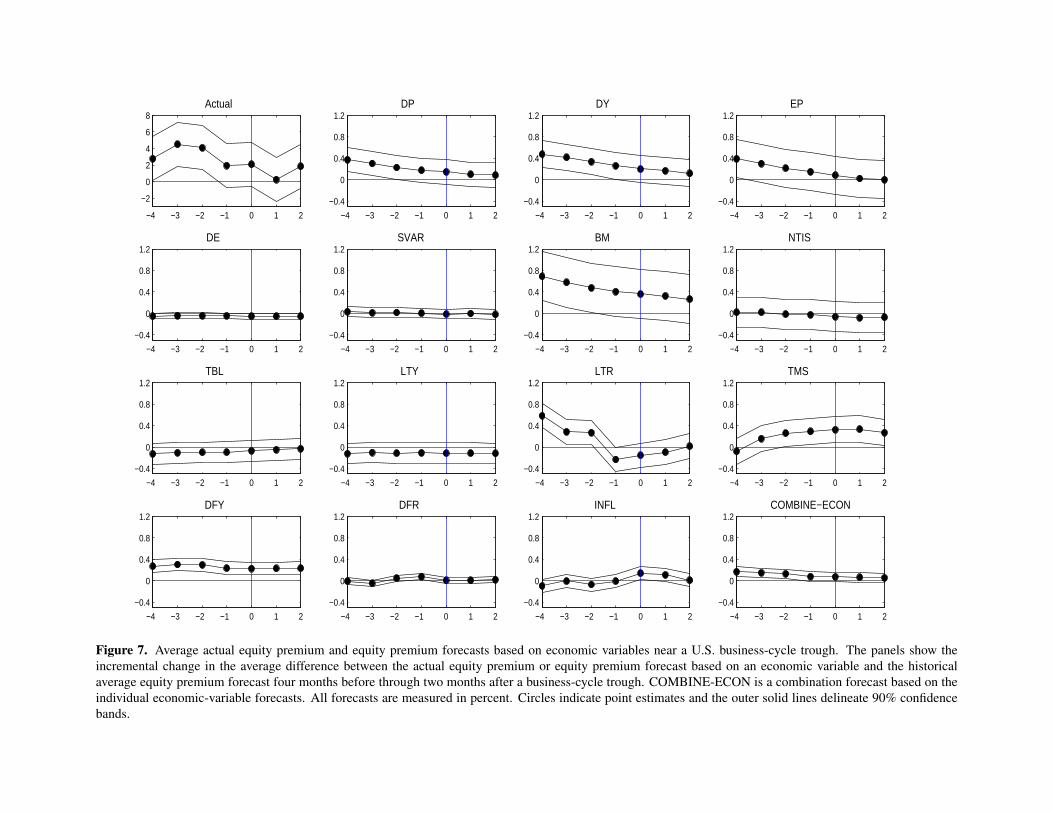
−4 −3 −2 −1 0 1 2

−2

0

2

4

6

8Actual

−4 −3 −2 −1 0 1 2

−0.4

0

0.4

0.8

1.2DP

−4 −3 −2 −1 0 1 2

−0.4

0

0.4

0.8

1.2DY

−4 −3 −2 −1 0 1 2

−0.4

0

0.4

0.8

1.2EP

−4 −3 −2 −1 0 1 2

−0.4

0

0.4

0.8

1.2DE

−4 −3 −2 −1 0 1 2

−0.4

0

0.4

0.8

1.2SVAR

−4 −3 −2 −1 0 1 2

−0.4

0

0.4

0.8

1.2BM

−4 −3 −2 −1 0 1 2

−0.4

0

0.4

0.8

1.2NTIS

−4 −3 −2 −1 0 1 2

−0.4

0

0.4

0.8

1.2TBL

−4 −3 −2 −1 0 1 2

−0.4

0

0.4

0.8

1.2LTY

−4 −3 −2 −1 0 1 2

−0.4

0

0.4

0.8

1.2LTR

−4 −3 −2 −1 0 1 2

−0.4

0

0.4

0.8

1.2TMS

−4 −3 −2 −1 0 1 2

−0.4

0

0.4

0.8

1.2DFY

−4 −3 −2 −1 0 1 2

−0.4

0

0.4

0.8

1.2DFR

−4 −3 −2 −1 0 1 2

−0.4

0

0.4

0.8

1.2INFL

−4 −3 −2 −1 0 1 2

−0.4

0

0.4

0.8

1.2COMBINE−ECON

Figure 7. Average actual equity premium and equity premium forecasts based on economic variables near a U.S. business-cycle trough. The panels show theincremental change in the average difference between the actual equity premium or equity premium forecast based on an economic variable and the historicalaverage equity premium forecast four months before through two months after a business-cycle trough. COMBINE-ECON is a combination forecast based on theindividual economic-variable forecasts. All forecasts are measured in percent. Circles indicate point estimates and the outer solid lines delineate 90% confidencebands.

−4 −3 −2 −1 0 1 2

−2

0

2

4

6

8Actual

−4 −3 −2 −1 0 1 2

−0.6

−0.3

0

0.3

0.6

MA(1,3)

−4 −3 −2 −1 0 1 2

−0.6

−0.3

0

0.3

0.6

MA(1,6)

−4 −3 −2 −1 0 1 2

−0.6

−0.3

0

0.3

0.6

MA(1,9)

−4 −3 −2 −1 0 1 2

−0.6

−0.3

0

0.3

0.6

MA(1,12)

−4 −3 −2 −1 0 1 2

−0.6

−0.3

0

0.3

0.6

MA(1,15)

−4 −3 −2 −1 0 1 2

−0.6

−0.3

0

0.3

0.6

MA(1,18)

−4 −3 −2 −1 0 1 2

−0.6

−0.3

0

0.3

0.6

MA(1,21)

−4 −3 −2 −1 0 1 2

−0.6

−0.3

0

0.3

0.6

MA(1,24)

−4 −3 −2 −1 0 1 2

−0.6

−0.3

0

0.3

0.6

MA(2,3)

−4 −3 −2 −1 0 1 2

−0.6

−0.3

0

0.3

0.6

MA(2,6)

−4 −3 −2 −1 0 1 2

−0.6

−0.3

0

0.3

0.6

MA(2,9)

−4 −3 −2 −1 0 1 2

−0.6

−0.3

0

0.3

0.6

MA(2,12)

−4 −3 −2 −1 0 1 2

−0.6

−0.3

0

0.3

0.6

MA(2,15)

−4 −3 −2 −1 0 1 2

−0.6

−0.3

0

0.3

0.6

MA(2,18)

−4 −3 −2 −1 0 1 2

−0.6

−0.3

0

0.3

0.6

MA(2,21)

−4 −3 −2 −1 0 1 2

−0.6

−0.3

0

0.3

0.6

MA(2,24)

−4 −3 −2 −1 0 1 2

−0.6

−0.3

0

0.3

0.6

COMBINE−MA

Figure 8. Average actual equity premium and equity premium forecasts based on moving-average rules near a U.S. business-cycle trough. The panels showthe incremental change in the average difference between the actual equity premium or equity premium forecast based on a moving-average rule and the historicalaverage equity premium forecast four months before through two months after a business-cycle trough. COMBINE-MA is a combination forecast based on theindividual moving-average forecasts. All forecasts are measured in percent. Circles indicate point estimates and the outer solid lines delineate 90% confidencebands.