Oum, Oren and Deng, March 24, 20061 Hedging Quantity Risks with Standard Power Options in a...

Oum, Oren and Deng, March 24, 2006

1

Hedging Quantity Risks with Standard Power Options in a Competitive Electricity Market

Yumi Oum, University of California at BerkeleyShmuel Oren, University of California at BerkeleyShijie Deng, Georgia Institute of Technology

Eleventh Annual POWER Research ConferenceBerkeley, CA, March 24, 2006


2

Electricity Supply Chain

Wholesale electricity market

(spot market)

LSE(load serving

entity)

Customers(end users servedat fixed regulated

rate)

Generators


3

Volumetric Risk for Load-Serving Entities Properties of electricity demand (load)

Uncertain and unpredictable Weather-driven volatile

Sources of LSEs exposure Highly volatile spot price Flat (regulated) retail rates & limited demand response Electricity is non-storable (no inventory) Electricity demand has to be served (no “busy signal”) Adversely correlated wholesale price and demand

Covering expected load with forward contracts will result in a contract deficit when prices are high and contract excess when prices are low so the LSE faces net revenue exposure due to demand fluctuations


4

Price and Demand CorrelationElectricity Demand and Price in California

0

2000

4000

6000

8000

10000

12000

14000

16000

18000

9, July ~ 16, July 1998

Dem

and

(M

W)

0

20

40

60

80

100

120

140

160

180

Electricity P

rice ($/MW

h)

Load

Price

Correlation coefficients:

0.539 for hourly price and load from 4/1998 to 3/2000 at Cal PX

0.7, 0.58, 0.53 for normalized average weekday price and load in Spain, Britain, and Scandinavia, respectively


5

Tools for Volumetric Risk Management Electricity derivatives

Forward or futures Plain-Vanilla options (puts and calls) Swing options (options with flexible exercise rate)

Temperature-based weather derivatives Heating Degree Days, Cooling Degree Days

Power-weather Cross Commodity derivatives Payouts when two conditions are met (e.g. both high

temperature & high spot price) Demand response Programs

Interruptible Service Contracts Real Time Pricing


6

Scope of This Work

Finding an optimal net revenue-hedging strategy for an LSE using plain electricity derivatives and forward contracts Exploit the correlation between electricity spot price and power

demand in volumetric risk management Characterize an “optimal” exotic hedging instrument Demonstrate the exposure reduction with an optimal exotic hedge Replication of the optimal hedge with forward contracts and

standard European call and put options Sensitivity analysis with respect to model parameters.


7

Model Setup One-period model

At time 0: construct a portfolio with payoff x(p) At time 1: hedged profit Y(p,q,x(p)) = (r-p)q+x(p)

Objective Find a zero cost portfolio with exotic payoff which maximizes

expected utility of hedged profit under no credit restrictions.

Spot market

LSE Load (q)

p r

Portfolio

x(p)

for a delivery at time 1


8

Mathematical Formulation

Objective function

Constraint: zero-cost constraint

dqdpqpfpxqprU

pxqprUE

px

px

),()]()[(max

)]()[(max

)(

)(

Utility function over profit

Joint distribution of p and q

0)]([1

pxEB

Q

Q: risk-neutral probability measure

B : price of a bond paying $1 at time 1

! A contract is priced as an expected discounted payoff under risk-neutral measure


9

Optimality Condition

)(

)(*|)(*)('

pf

pgppxqprUE

p

The Lagrangian multiplier is determined so that the constraint is satisfied

Utility functions we examine CARA (constant absolute risk aversion) utility function:

Mean-variance utility function:

aYea

YU 1

)(

)(2

1][)]([ YaVarYEYUE


10

Optimal Payoff Functions Obtained

]|[ln]|[ln

)(

)(ln

)(

)(ln

1)(* ),(),( peEEpeE

pg

pfE

pg

pf

apx qpayQqpaypQp

With a CARA utility function

With a Mean-variance utility function:

]|),([

)()(

)()(

]]|),([[

)()(

)()(

11

)(* pqpyE

pfpg

E

pfpg

pqpyEE

pfpg

E

pfpg

apx

p

Q

pQ

p

Q

p


11

Assumptions on distributions We consider two different joint distributions for price and

demand:

Bivariate lognormal-normal distribution:

Bivariate lognormal distribution:

),(~log:

),(log),,(~),,(~log:2

2

221

smNpQUnder

qpCorrumNqsmNpPUnder

),(~log:

)log,(log),,(~log),,(~log:2

2

221

smNpQUnder

qpCorrumNqsmNpPUnder qq


12

Optimal Exotic Payoff Bivariate lognormal-normal distribution:

For a CARA utility

For a mean-variance utility

)1()(22

1)(log

))(()(log)(log1

)(*

222222

1

2

12

2

2

1

122212

22

22

22

22

uepepraesmpps

u

epms

ummp

s

urmp

s

mm

apx

smsmsm

sm

22

222

122

2121

212

22121

2

12

2212

12

)3)((

12

)3)((

)(

)(log)(11

)(*

smsms

mm

s

mmmm

s

mm

s

mmmm

esmrms

um

s

umerpe

mps

umprpe

apx

),(~log:

),(log),,(~),,(~log:2

2

221

smNpQUnder

qpCorrumNqsmNpPUnder


13

Optimal Exotic Payoff Bivariate lognormal distribution:

For a mean-variance utility

22

221222222

12212

22121

2212

122

2121

12

1)1(

2

1)(

2

1)1(

2

1)(

2

)3)((

)1(2

1)(log

2

)3)((

)(11

)(*

ss

uumm

s

ummuumm

s

um

s

mm

s

mmmm

umps

um

s

mm

s

mmmm

qq

qq

qqq

q

qq

q

erepe

eprpea

px

),(~log:

)log,(log),,(~log),,(~log:2

2

221

smNpQUnder

qpCorrumNqsmNpPUnder qq


14

0 50 100 150 200 250

-2

0

2

4

6

8x 10

4

Spot price p

x*(p

)

=0 =0.3 =0.5 =0.7 =0.8

0 50 100 150 200 250-2

-1

0

1

2

3

4x 10

7

Spot price p

x*(p

)

=0 =0.3 =0.5 =0.7 =0.8

Illustrations of Optimal Exotic Payoffs

0 50 100 150 200 250 3000

0.002

0.004

0.006

0.008

0.01

0.012

0.014

Price p

Pro

babi

lity

-5 0 5

x 104

0

1

2

3

4

5

6

7x 10

-5

profit: y = (r-p)q + x(p)

Pro

babi

lity

= 0 = 0.3 = 0.5 = 0.7 = 0.8

rate) retail(flat /120$

60)(,300][

/56$)(,/70$][

),30,300,7.0,4(~),(log 22,

MWhr

MWhqMWhqE

MWhpMWhpE

NqpQP

Bivariate lognormal-normal distributionDist’n of p

Dist’n of profit

r

Optimal exotic payoff

CARA Mean-Var


15

-5 0 5

x 104

0

1

2

3

4

5

6

7

8x 10

-5

profit: y = (r-p)q + x(p)

Pro

babi

lity

= 0 = 0.3 = 0.5 = 0.7 = 0.8

Illustrations of Optimal Exotic Payoffs

rate) retail(flat /120$

60)(,300][

/56$)(,/70$][

Q&Punder ),2.0,69.5,7.0,4(~)log,(log 22

MWhr

MWhqMWhqE

MWhpMWhpE

Nqp

Bivariate lognormal distribution: Dist’n of profit

Optimal exotic payoff

Mean-Var

E[p]

Note: For the mean-variance utility, the optimal payoff is linear in p when correlation is 0,

0 50 100 150 200 250

-2

0

2

4

6

8x 10

4

Spot price p

x*(p

)

=0 =0.3 =0.5 =0.7 =0.8

Mean-Var


16

-1 -0.5 0 0.5 1 1.261.5 2 2.5 3

x 104

0

0.5

1

1.5

2

2.5

3x 10

-4

Profit

Pro

babi

lity

After price & quantity hedge

After price hedge

Before hedge

-1 -0.5 0 0.5 1 1.281.5 2 2.5 3

x 104

0

0.5

1

1.5

2

2.5

3x 10

-4

Profit

Pro

babi

lity

After price & quantity hedge

After price hedge

Before hedge

Volumetric-hedging effect on profit dist’n

Bivariate lognormal for (p,q)Bivariate lognormal-normal for (p,q)

Comparison of profit distribution for an LSE with mean-variance utility (ρ=0.8) Price hedge: optimal forward hedge Price and quantity hedge: optimal exotic hedge


17

0 50 100 150 200 250-6

-4

-2

0

2

4

6

8

10

12x 10

6

Spot price p

x*(p

)

m2 = m1-0.1m2 = m1-0.05m2 = m1m2 = m1+0.05m2 = m1+0.1

0 50 100 150 200 250-2

-1

0

1

2

3

4

5

6

7x 10

4

Spot price p

x*(p

)

m2 = m1-0.1m2 = m1-0.05m2 = m1m2 = m1+0.05m2 = m1+0.1

Sensitivity to market risk premium

With Mean-variance utility (a =0.0001) With CARA utility

1.0,1.77

05.0,3.73

0,8.69

05.0,4.66

1.0,1.63

][

12

12

12

12

12

mmif

mmif

mmif

mmif

mmif

pEQ][log2 pEm Q


18

0 50 100 150 200 250-1

-0.5

0

0.5

1

1.5x 10

7

Spot price p

x*(p

)

a =0.1a =0.5a =1a =1.5a =2

0 50 100 150 200 250-5

0

5

10

15

20x 10

4

Spot price p

x*(p

)

a =5e-006a =1e-005a =5e-005a =0.0001a =0.001

Sensitivity to risk-aversion

with mean-variance utility (m2 = m1+0.1) with CARA utility

Optimal payoffs by risk aversion

aYea

YU 1

)( )(2

1][)]([ YaVarYEYUE

(Bigger ‘a’ = more risk-averse)

Note: if m1 = m2 (i.e., P=Q), ‘a’ doesn’t matter for the mean-variance utility.


19

We’ve obtained an exotic payoff function that we like to replicate with standard forward contracts plus a portfolio of call and put options.

Carr and Madan(2001) showed any twice continuously differentiable function can be written as:

Replication ( s forward price F)

Replication with Standard Instruments

dKKpKxdKpKKxFpFxFxpxF

F

))((''))((''))(('1)()(

0

Forward payoff

Put option payoff

Call option payoff

Bond payoff

Strike < F

Strike > F

Payoff

p

Forward price

F

Payoff

K

Payoff

Strike price

K

Strike price

dKKpKxdKpKKxpsxssxsxpxs

s

))((''))(('')('])(')([)(

0


20

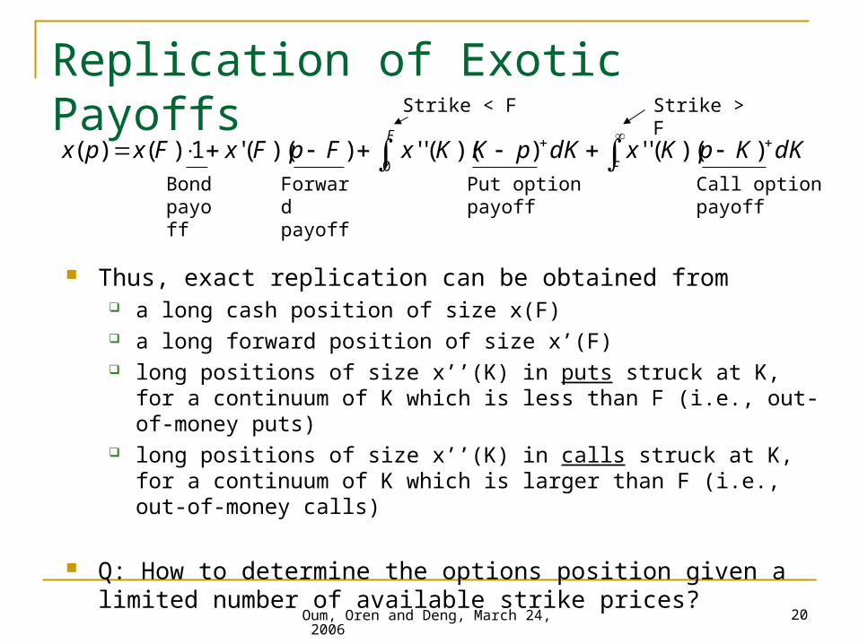
Replication of Exotic Payoffs

dKKpKxdKpKKxFpFxFxpxF

F

))((''))((''))(('1)()(

0

Forward payoff

Put option payoff

Call option payoff

Bond payoff

Strike < F Strike > F

Thus, exact replication can be obtained from a long cash position of size x(F) a long forward position of size x’(F) long positions of size x’’(K) in puts struck at K, for a continuum of K

which is less than F (i.e., out-of-money puts) long positions of size x’’(K) in calls struck at K, for a continuum of K

which is larger than F (i.e., out-of-money calls)

Q: How to determine the options position given a limited number of available strike prices?


21

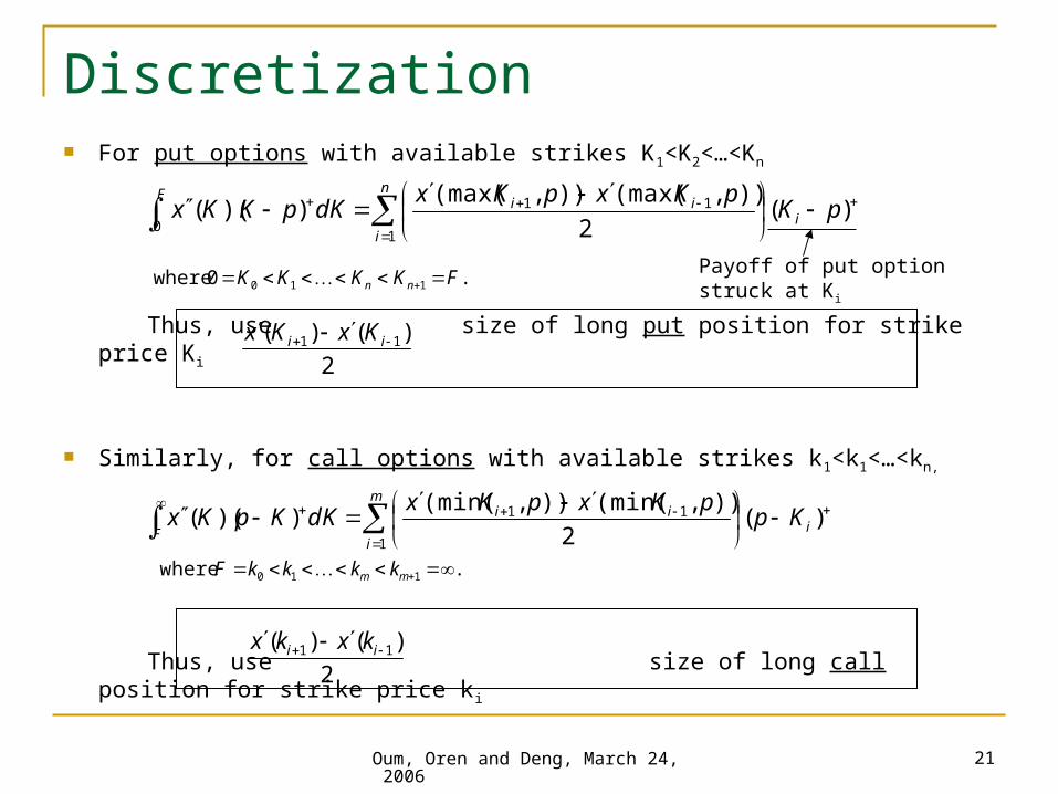
For put options with available strikes K1<K2<…<Kn

Thus, use size of long put position for strike price Ki

Similarly, for call options with available strikes k1<k1<…<kn,

Thus, use size of long call position for strike price ki

Discretization

n

ii

iiF

pKpKxpKx

dKpKKx1

11

0)(

2

)),(max()),(max())((

Payoff of put option struck at Ki.0where 110 FKKKK nn

m

ii

ii

FKp

pKxpKxdKKpKx

1

11 )(2

)),(min()),(min())((

.where 110 mm kkkkF

2

)()( 11 ii KxKx

2

)()( 11 ii kxkx


22

0 50 100 150 200 250-6

-4

-2

0

2

4

6

8

10

12x 10

6

Spot price p

payo

ff

x*(p)Replicated when K = $1Replicated when K = $5Replicated when K = $10

0 50 100 150 200 250-8

-6

-4

-2

0

2

4

6

8x 10

5

Spot price p

x*'(p

)

=0 =0.3 =0.5 =0.7 =0.8

0 50 100 150 200 2500

1000

2000

3000

4000

5000

6000

7000

8000

Spot price p

x*''(

p)

=0 =0.3 =0.5 =0.7 =0.8

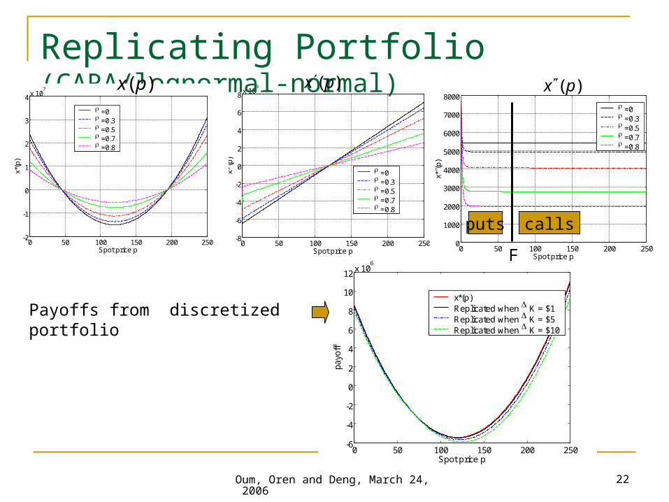
Replicating Portfolio (CARA/lognormal-normal))( px )( px

puts calls

Payoffs from discretized portfolio

0 50 100 150 200 250-2

-1

0

1

2

3

4x 10

7

Spot price p

x*(p

)

=0 =0.3 =0.5 =0.7 =0.8

F

)( px


23

0 50 100 150 200 250

-2

0

2

4

6

8x 10

4

Spot price p

x*(p

)

=0 =0.3 =0.5 =0.7 =0.8

0 50 100 150 200 250-400

-300

-200

-100

0

100

200

300

400

500

Spot price p

x*'(p

) =0 =0.3 =0.5 =0.7 =0.8

0 50 100 150 200 2500

2

4

6

8

10

Spot price p

x*''(

p)

=0 =0.3 =0.5 =0.7 =0.8

Replicating Portfolio (MV/lognormal-normal))( px )( px )( px

puts calls

F


0 50 100 150 200 250-2

-1

0

1

2

3

4

5

6

7x 10

4

Spot price p

payo

ff



24

0 50 100 150 200 250-2

-1

0

1

2

3

4

5

6

7x 10

4

Spot price p

payo

ff


0 50 100 150 200 250

-2

0

2

4

6

8x 10

4

Spot price p

x*(p

)

=0 =0.3 =0.5 =0.7 =0.8

0 50 100 150 200 250-500

0

500

Spot price p

x*'(p

)

=0 =0.3 =0.5 =0.7 =0.8

0 50 100 150 200 2500

10

20

30

40

50

60

Spot price p

x*''(

p)

=0 =0.3 =0.5 =0.7 =0.8

Replicating Portfolio (MV/lognormal-lognormal))( px )( px )( px

puts calls

F



25

Conclusion We have constructed an optimal portfolio for hedging the

increased exposure due to correlated price and volumetric risk for LSEs Forward contracts plus a spectrum of call and put options

We have shown a good way of replicating exotic options with available call and put options given discrete strike prices.

The results obtained with an optimal hedging portfolio provide a useful benchmark for simpler hedging strategies.

Extensions Decide the best hedging timing Use Value-at-Risk measure

Optimal hedging under credit limit constraints05.0})(),({..

)](),([)(

VaRpxqpPts

pxqpEMaxpx

Oum, Oren and Deng, March 24, 20061 Hedging Quantity Risks with Standard Power Options in a...

Documents

Transcript of Oum, Oren and Deng, March 24, 20061 Hedging Quantity Risks with Standard Power Options in a...