Orthonormal bases of compactly supported waveletsingrid/publications/cpam41-1988.pdfOrthonormal...
88
Orthonormal Bases of Compactly Supported Wavelets INGRID DAUBECHIES A T&T Bell Laboratories Abstract We construct orthonormal bases of compactly supported wavelets, with arbitrarily high regular- ity. The order of regularity increases linearly with the support width. We start by reviewing the concept of multiresolution analysis as well as several algorithms in vision decomposition and reconstruction. The construction then follows from a synthesis of these different approaches. 1. Introduction In recent years, families of functions h4. 6, a, b E W, a # 0, generated from one single function h by the operation of dilations and transla- tions, have turned out to be a useful tool in many different fields of mathematics, pure as well as applied. Following Grossmann and Morlet [l], we shall call such families “wavelets”. Techniques based on the use of translations and dilations are certainly not new. They can be traced back to the work of A. Calderbn [2] on singular integral operators, or to renormalization group ideas (see [3]) in quantum field theory and statistical mechanics. Even in these two disciplines, however, the explicit intro- duction of special families of wavelets seems to have led to new results (see, e.g. [4],[5],[6]). Moreover, wavelets are useful in many other applications as well. They are used for e.g. sound analysis and reconstruction in [7], and have led to a new algorithm, with many attractive features, for the decomposition of visual data in [8]. They seem to hold great promise for the detection of edges and singularities; see [9]. It is therefore fair to surmise that they will have applications in yet other directions. Depending on the type of application, different families of wavelets may be chosen. One can choose, e.g., to let the parameters a, b in (1.1) vary continuously on their range W* X R (where R* = R \ (0)). One can then, for instance, represent functions f E L2(W) by the functions Uf, Communications on Pure and Applied Mathematics, Vol. XLI 909-996 (1988) 6 1988 John Wiley & Sons, Inc. CCC 0010-3640/88/070909-88$04.00
Transcript of Orthonormal bases of compactly supported waveletsingrid/publications/cpam41-1988.pdfOrthonormal...
Orthonormal Bases of Compactly Supported Wavelets
INGRID DAUBECHIES A T&T Bell Laboratories
Abstract
We construct orthonormal bases of compactly supported wavelets, with arbitrarily high regular- ity. The order of regularity increases linearly with the support width. We start by reviewing the concept of multiresolution analysis as well as several algorithms in vision decomposition and reconstruction. The construction then follows from a synthesis of these different approaches.
1. Introduction
In recent years, families of functions h4. 6 ,
a , b E W, a # 0,
generated from one single function h by the operation of dilations and transla- tions, have turned out to be a useful tool in many different fields of mathematics, pure as well as applied. Following Grossmann and Morlet [l], we shall call such families “wavelets”.
Techniques based on the use of translations and dilations are certainly not new. They can be traced back to the work of A. Calderbn [2] on singular integral operators, or to renormalization group ideas (see [3]) in quantum field theory and statistical mechanics. Even in these two disciplines, however, the explicit intro- duction of special families of wavelets seems to have led to new results (see, e.g. [4],[5],[6]). Moreover, wavelets are useful in many other applications as well. They are used for e.g. sound analysis and reconstruction in [7], and have led to a new algorithm, with many attractive features, for the decomposition of visual data in [8]. They seem to hold great promise for the detection of edges and singularities; see [9]. It is therefore fair to surmise that they will have applications in yet other directions.
Depending on the type of application, different families of wavelets may be chosen. One can choose, e.g., to let the parameters a , b in (1.1) vary continuously on their range W* X R (where R * = R \ (0)). One can then, for instance, represent functions f E L2(W) by the functions Uf,
Communications on Pure and Applied Mathematics, Vol. XLI 909-996 (1988) 6 1988 John Wiley & Sons, Inc. CCC 0010-3640/88/070909-88$04.00
910 I. DAUBECHIES
If h satisfies the condition
where denotes the Fourier transform,
then U (as defined by (1.2)) is an isometry (up to a constant) from L2(R) into L2(W* x W; da db). The map U is called the “continuous wavelet transform”; see [1],[10]. In this form, wavelets are closest to the original work of Calderbn. The continuous wavelet transform is also closely related to the “afline coherent state representation” of quantum mechanics (first constructed in [ll], see also [12]); in fact, for appropriate choices of h, the h@, are “affine coherent states”, and have been used in the study of some quantum mechanics problems in
Note that the “admissibility condition” (1.3) implies, if h has sufficient decay [111, [121.
which we shall always assume in practice, that h has mean zero,
(1 -4) J d x h ( x ) = 0.
Typically, the function h will therefore have at least some oscillations. A standard example is
For other applications, including those in signal analysis, one may choose to restrict the values of the parameters a, b in (1.1) to a discrete sublattice. In this case one fixes a dilation step a, > 1, and a translation step b, # 0. The family of wavelets of interest becomes then, for m, n E Z,
(1.6) h , , ( x ) = - nb,).
Note that this corresponds to the choices
a = a,“,
b = nb,a,”,
indicating that the translation parameter b depends on the chosen dilation rate. For m large and positive, the oscillating function h,, is very much spread out, and the large translation steps boa,” are adapted to this wide width. For large but
ORTHONORMAL. BASES OF WAVELETS 91 1
negative m the opposite happens; the function h,, is very much concentrated, and the small translation steps boa,” are necessary to still cover the whole range.
A “discrete wavelet transform” T is associated with the discrete wavelets (1.6). It maps functions f to sequences indexed by Z2,
If h is “admissible”, i.e., if h satisfies the condition (1.3), and if h has sufficient decay, then T maps L2(R) into 12(Z2) . In general, T does not have a bounded inverse on its range. If it does, i.e., if, for some A > 0, B < 00,
for all f in L2(W), then the set { hmn; rn, n E H} is called a “frame”. In this case one can construct numerically stable algorithms to reconstruct f from its wavelet coefficients (h,,, f). In particular,
with
For B / A close to 1, which is the case in the decompositions and reconstructions of music and other sound signals, as done by A. Grossmann, R. Kronland and J. Morlet [7], the “error term” R can be omitted. In practice, with e.g. the basic wavelet (lS), and with a, = 21/4, b, = .5, one finds B / A - 1 < lop5, and the reconstruction formula (1.8) restricted to its first term gives excellent results. In fact, even for the larger value a, = 2, corresponding to B / A - 1 = .08, the truncated reconstruction formula, when applied to the wavelet decomposition of speech signals, leads to a clearly understandable reconstruction; see [13].
In the use of wavelet frames for sound analysis, and reconstruction, as studied by the Marseilles group [7], the families of wavelets h,, considered are highly redundant, i.e., they are not independent, in the sense that any finite number of them lies in the closed linear span generated by the others. Consequently, the range of the discrete wavelet transform T is a proper subspace of 12(Z2). The higher the redundancy of the frame, the smaller this subspace, which is a desirable feature for some purposes (e.g. the reduction of calculational noise). If a,, b, are chosen very close to 1,0, respectively, then the resulting frame is very
912 I. DAUBECHIES
redundant and very close to the continuous family of wavelets (1.1); this type of frame was used in the “edge detection” study mentioned earlier; see [9].
For other applications, as e.g. in S. Mallat’s vision decomposition algorithm in [8], it is preferable to work with the other extremum, and to reduce re- dundancy as much as possible. In this case, one can turn to choices of h and a,, b, (typically a, = 2) for which the h,, constitute an orthonormal basis. This is the case to which we shall be restricting ourselves in the remainder of this paper. For a more detailed study of general (non-orthonormal) wavelet frames, and a discussion of the similarities and the differences between wavelet transform and windowed Fourier transform, the reader is referred to [14], [15].
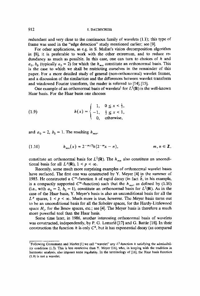
One example of an orthonormal basis of wavelets’ for L2(R) is the well-known Haar basis. For the Haar basis one chooses
1, o j x < + , -1, f s x < l ,
0, otherwise,
and a, = 2, b, = 1. The resulting h,,,
(1.10) h , , ( x ) = 2-”’%(2-”x - n ) , m , n E Z,
constitute an orthonormal basis for L2(W). The h,, also constitute an uncondi- tional basis for all LP(R), 1 < p < 00.
Recently, some much more surprising examples of orthonormal wavelet bases have surfaced. The first one was constructed by Y. Meyer [4] in the summer of 1985. He constructed a C“-function h of rapid decay (in fact h, in his example, is a compactly supported Cm-function) such that the h,,, as defined by (1.10) (i.e., with a , = 2, b, = l), constitute an orthonormal basis for L2(W). As in the case of the Haar basis, Y. Meyer’s basis is also an unconditional basis for all the LP spaces, 1 < p < 00. Much more is true, however. The Meyer basis turns out to be an unconditional basis for all the Sobolev spaces, for the Hardy-Littlewood space H I , for the Besov spaces, etc.; see [4]. The Meyer basis is therefore a much more powerful tool than the Haar basis.
Some time later, in 1986, another interesting orthonormal basis of wavelets was constructed, independently, by P. G. LemariB [17] and G. Battle [18]. In their construction the function h is only Ck, but it has exponential decay (as compared
‘Following Grossmann and Morlet [ l] we call “wavelet” any L2-function h satisfying the admissibil- ity condition (1.3). This is less restrictive than Y. Meyer [16], who, in keeping with the tradition in harmonic analysis, also imposes some regularity. In the terminology of [16], the Haar basis function (1.9) is not a wavelet.
ORTHONORMAL BASES OF WAVELETS 913
with decay faster than any power in Y. Meyer’s case). It also has k vanishing moments, i.e.,
I d X X ’ h ( X ) = 0, j = O , l , * . * , k - 1,
which makes these h,, an unconditional basis for all the Sobolev spaces 2$, with
In all these constructions the choices a, = 2, b, = 1 were made. The choice for b, is of course arbitrary, a simple dilation of the function h allows one to fix any non-zero choice for b,; it is convenient to choose b, = 1. The choice of a, is far less arbitrary. We shall restrict ourselves here to a, = 2, although it is possible to consider other, though by no means arbitrary, choices for a, (see
In the fall of 1986, S. Mallat and Y. Meyer [16],[19] realized that these different wavelet basis constructions can all be realized by a “multiresolution analysis”. This is a framework in which functions f E L2(Wd) can be considered as a limit of successive approximations, f = lim, ~ - P, f, where the different P, f, m E Z, correspond to smoothed versions of f, with a “smoothing out action radius” of the order of 2”’. The wavelet coefficients (h,,, f ), with fixed m, then correspond to the difference between the two successive approximations P, - f and P, f. A more detailed description of multiresolution analysis will be given in Section 2.
The concept of multiresolution analysis plays a central role in S. Mallat’s algorithm for the decomposition and reconstruction of images in [8]. In fact, ideas related to multiresolution analysis (a hierarchy of averages, and the study of their differences) were already present in an older algorithm for image analysis and reconstruction, namely the Laplacian pyramid scheme of P. Burt and E. Adelson [20]. The Laplacian pyramid ideas triggered S. Mallat to view the orthonormal bases of wavelets as a vehicle for multiresolution analysis. Together, S. Mallat and Y. Meyer then carried out a more detailed mathematical analysis, showing how all the “accidental” previous constructions found their natural framework in multiresolution analysis; see [16], [19]. By the use of multiresolution analysis and orthonormal wavelet bases, S. Mallat constructed an algorithm that is both more economical and more powerful in its orientation selectivity. On the other hand, by a curious feedback, the combination of Mallat’s ideas and of the restrictions on “filters” imposed in [20] led to my construction of orthonormal wavelet bases of compact support, which is the main topic of this paper.
Because of the important role, in the present construction, of the interplay of all these different concepts, and also to give a wider publicity to them, an extensive review will be given in Section 2 of multiresolution analysis (subsection 2A), of the Laplacian pyramid scheme (subsection 2B) and of Mallat’s algorithm (subsection 2C).
Sections 3 and 4 contain the new results of this paper. A closer look at Mallat’s work shows that he uses the intermediary of orthonormal wavelet bases
s < k - l .
[41,1211).
914 I. DAUBECHIES
for function spaces to build an essentially discrete algorithm. It seemed therefore natural to wonder whether similar, and as powerful, discrete algorithms could be built directly, without using function spaces as an intermediate step. It turns out that it is very easy to write a set of necessary and sufficient conditions, on the “discrete side”, ensuring that an algorithm similar to Mallat’s works. This is done in subsection 3A. In order to have a useful algorithm, however, an extra regularity condition has to be imposed (this condition is already satisfied in e.g. Burt and Adelsen’s Laplacian pyramid scheme). This is done in subsection 3B. The combination of the discrete conditions and the regularity condition on the discrete algorithm turns out, however, to be strong enough to impose an underly- ing multiresolution analysis of functions, with associated orthonormal wavelet basis. Provided the regularity condition is satisfied, there is therefore a one-to-one correspondence between orthonormal wavelet bases and discrete multiresolution decompositions, in the sense of Mallat’s algorithm. This equivalence is proved in subsection 3C. Another proof of the same result, using different techniques, can be found in [19]; the proof presented here is more “graphical”, and closer to the “filter” point of view of [20].
In Section 4, we exploit the equivalence between discrete and function schemes to build orthonormal bases of wavelets with compact support. Using this equivalence, it turns out that it is sufficient to build a discrete scheme using filters with a finite number of taps. This can be done explicitly, as shown in subsection 4B. As a result one can construct, for any k E N, a Ck-function + with compact support, such that the corresponding +,,,
+&) = 2-”’751(2-”x - n), constitute an orthonormal basis. The size of the support increases linearly with the regularity. Moreover, + has K consecutive moments equal to zero,
JdXxi+(x) = 0, j = O , l , * . - , K - 1,
where K also increases linearly with k. All these properties of the construction are proved in subsection 4C. Finally, the “graphical” approach which, as ex- plained in subsection 3B, was the guideline to the proof of the link between the “regularity” condition of Burt and Adelson (see subsection 2B) and multiresolu- tion analysis, can also be used to plot the functions +. We conclude this paper with the plots of a few of the compactly supported wavelets constructed here.
2. Multiresolution Analysis and Image Decomposition and Reconstruction
2.A. A review of multiresolution analysis and orthonormal wavelet bases. In this subsection we review the definition of multiresolution analysis, and show how orthonormal bases of wavelets can be constructed starting from a multireso- lution analysis. We illustrate this construction with examples. No proofs will be given; for proofs, more details and generalizations we refer to [16], [19] or [21].
ORTHONORMAL BASES OF WAVELETS 915
The idea of a multiresolution analysis is to write L2-functions f as a limit of successive approximations, each of which is a smoothed version of f, with more and more concentrated smoothing functions. The successive approximations thus use a different resolution, whence the name multiresolution analysis. The succes- sive approximation schemes are also required to have some translational invari- ance. More precisely, a multiresolution analysis consists of
(i) a family of embedded closed subspaces V, C L2(W), m E h,
(2.1) * * - c V 2 c V l c V o c V ~ , c V ~ , c * . .
such that (ii)
n V, = (01, m= LYW), rn€Z ,€Z
(2.2)
and (iii)
(2.3) f E V, *f(2 *) E Vm-l;
moreover, there is a + E Vo such that, for all m E H, the +ffln constitute an unconditional basis for V,, that is, (iv)
(2.4a) V, = linear span { +,,, n E Z}
and there exist 0 < A 6 B < co such that, for all ( c J n G z E 12(h), 2
(2.4b) A C I C ~ I ~ ~ ~ ~ ~ ~ n + r n n l ~ s BClcnt2* n n
Here +,,(x) = 2-m/2+(2-"x - n). Let P, denote the orthogonal projection onto V,. It is then clear from (2.1), (2.2) that lim, -t -,P,f = f, for all f E L2(W). The condition (2.3) ensures that the V, correspond to different scales, while the translational invariance
is a consequence of (2.4).
EXAMPLE 2.1. A typical though crude example is the following. Take the V, to be spaces of piecewise constant functions,
V, = { f~ L ~ ( w ) ; fconstant on [2mn,2m(n + 1) [for all n E z} .
The conditions (2.1)-(2.3) are clearly satisfied. The projections P, are defined by
916 I. DAUBECHIES
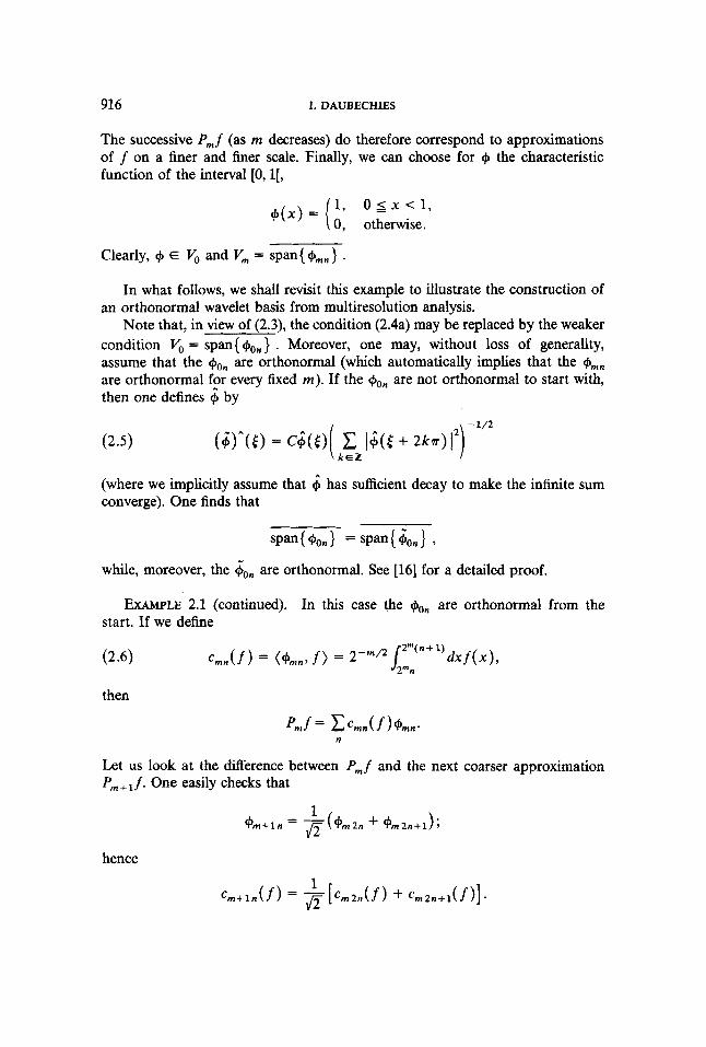
The successive P, f (as m decreases) do therefore correspond to approximations of f on a finer and finer scale. Finally, we can choose for + the characteristic function of the interval [0,1[,
1, O l X < l , 0, otherwise.
Clearly, + E Vo and V, = span{ +mn } .
In what follows, we shall revisit this example to illustrate the construction of an orthonormal wavelet basis from multiresolution analysis.
Note that, in view of (2.3), the condition (2.4a) may be replaced by the weaker condition Vo = span{ . Moreover, one may, without loss of generality, assume that the are orthonormal (which automatically implies that the cp,, are orthonormal for every fixed m). If the +on are not orthonormal to start with, then one defines 6 by
( i ) ^ C E ) = C $ W ( c J&E + 2 k d 12)-1'2 k c Z
(where we implicitly assume that $ has sufficient decay to make the infinite sum converge). One finds that
(2.5)
~
~
span{ +on 1 = span{ 6 O n } , while, moreover, the 6ofl are orthonormal. See [16] for a detailed proof.
EXAMPLE 2.1 (continued). In this case the +on are orthonormal from the start. If we define
then
P m f = C C m n ( f ) +mn* n
Let us look at the difference between P, f and the next coarser approximation P, + f. One easily checks that
hence
ORTHONORMAL BASES OF WAVELETS 917
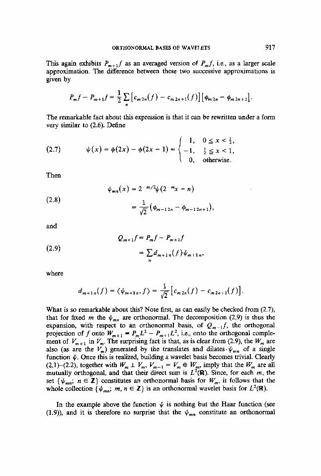
This again exhibits P,+l f as an averaged version of P, f, i.e., as a larger scale approximation. The difference between these two successive approximations is given by
The remarkable fact about this expression is that it can be rewritten under a form very similar to (2.6). Define
1, o s x < + ,
-1, + 5 x < 1, +(XI = + ( 2 4 - d 2 x - 1) =
0, otherwise. (2.7)
Then
and
(2 -9)
where
What is so remarkable about this? Note first, as can easily be checked from (2.7), that for fixed m the +mn are orthonormal. The decomposition (2.9) is thus the expansion, with respect to an orthonormal basis, of Q,-,f, the orthogonal projection of f onto W,+, = P,L2 - P,+,L2, i.e., onto the orthogonal comple- ment of Vm+, in V,. The surprising fact is that, as is clear from (2.9), the W, are also (as are the V , ) generated by the translates and dilates.+,, of a single function +. Once this is realized, building a wavelet basis becomes trivial. Clearly (2.1)-(2.2), together with W, I V,, Vm-l = V, CB W,, imply that the W, are all mutually orthogonal, and that their direct sum is L2(R). Since, for each m, the set { $mn; n E Z} constitutes an orthonormal basis for W,, it follows that the whole collection { +mn; m, n E h } is an orthonormal wavelet basis for L2(R).
In the example above the function + is nothing but the Haar function (see (1.9)), and it is therefore no surprise that the +,,,,, constitute an orthonormal
918 I. DAUBECHIES
basis. The example does however clearly show how this basis can be constructed from a multiresolution analysis. Let us sketch now how the general case works:
For a multiresolution analysis, i.e., a family of spaces V, and a function + satisfying (2.1)-(2.4), one defines (as in Example 2.1) W, as the orthogonal complement, in V,-,, of V,,
(2.10) Vm-, = V, a3 w,, w, I V,.
Equivalently,
(2.11) W, = Q,L2((W) with Q, = P,-1 - P,.
It follows immediately that all the W, are scaled versions of W,,
(2.12) f E w, - f(2" *) E w,, and that the W, are orthogonal spaces which sum to L2(R),
(2.13) L y R ) = @ w,. m € Z
Because of the properties (2.1)-(2.4) of the V,, it turns out (see [16],[19]) that in W, also (as in V,) there exists a vector + such that its integer translates span W,, i.e.,
where, as before, + m n ( ~ ) = 2-"/V(2-"x - n ) for m, n E E . It follows im- mediately from (2.12) that then
for all m E Z. Intuitively one may understand this similarity between W, and V, by the fact
that V- , is " twice as large" as V,, since V, is generated by the integer translates of a single function +oo, while V- , is generated by the integer translates of two functions, namely +-lo and +-ll. It therefore seems natural that the orthogonal complement W, of Vo in V - , is also generated by the integer translates of a single function. This hand-waving argument can easily be made rigorous by using group representation arguments. Mere proof of existence of a function + satisfy- ing (2.14) would however not be enough for practical purposes. A more detailed analysis leads to the following algorithm for the construction of J , (see [16], [19]). We start from a function + such that the +on are an orthonormal basis for Vo (if
ORTHONORMAL BASES OF WAVELETS 919
necessary, we apply (2.5)). Since 9 E V, C V - , = span{ 9(2 - n)} , there exist c, such that
(2.15)
Define then
The corresponding will constitute an orthonormal basis of W,; see [16], [19]. Consequently the I),,, for fixed m, will constitute an orthonormal basis of W,. It follows then from (2.12) that the {I),,, m, n E Z} constitute an orthonormal basis of wavelets for L2(W). This completes the explicit construction, in the general case, of an orthonormal wavelet basis from a multiresolution analysis.
EXAMPLE 2.1 (final visit). As we already noted above, the +,, are orthonor- mal in this example, and
$I(.) = 9(2x) + 9(2x - 1).
Applying the recipe (2.15)-(2.16) then leads to
which corresponds to (2.7).
Remarks. 1. One can show (see [MI) that the functions 9, J , having all the above properties necessarily satisfy
(2.17) /dx$(x) = 0
and
where we implicitly assume that 9, I) are sufficiently well-behaved for these integrals to make sense (in all examples of practical interest, 9, J , E L1). In fact, one does not even need to assume that the are orthonormal to derive (2.17)-(2.18). In [15] it is shown that (2.17) has to be satisfied even if the J,mn constitute only a frame (see the introduction). Note also that the transition (2.5) from 9 to 6, orthonormalizing the +,,, preserves j dx + ( x ) # 0.
2. If one restricts oneself to the case where 9 is a real function (as in all the examples above), then (p is determined uniquely, up to a sign, by the requirement
or
920 I. DAUBECHIES
that the sign of + so that
be orthonormal. One then also has j dx +(x) = fl; we shall fix the
(2.18) / d X + ( X ) = 1.
In practice, one can often start the whole construction by choosing an appro- priate +, i.e., a function @ satisfying (2.15) for some c,. Provided + is “reason; able” (it suffices, e.g., that infl t lsn(+(t) I > O and that &,,zl;(t + 2ka) I is bounded), the closed linear spans V, of the +,,, (rn fixed) then automatically satisfy (2.1)-(2.4) and there exists an associated orthonormal basis of wavelets. Two typical examples are
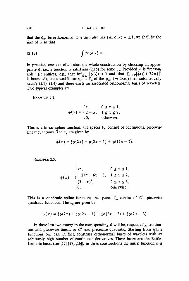
EXAMPLE 2.2.
O S X $ l , @(.)= 2 - x , 1 s x j 2 , I:: otherwise.
This is a linear spline function; the spaces V, consist of continuous, piecewise linear functions. The c, are given by
+(x) = ++(2x) + 442. - 1) + :+(h - 2).
EXAMPLE 2.3.
(xz, O S X $ l , - 2 ~ ’ + 6~ - 3, 1 5 x 5 2,
(3 - x)2, 2 5 x 5 3 , + ( X I =
10, otherwise.
This is a quadratic spline function; the spaces V, consist of C’, piecewise quadratic functions. The c, are given by
+(x) = $+(2x) + $+(2x - 1) + ;T+(2x - 2) + f+(2x - 3).
In these last two examples the corresponding + will be, respectively, continu- ous and piecewise linear, or C1 and piecewise quadratic. Starting from spline functions one can, in fact, construct orthonormal bases of wavelets with an arbitrarily high number of continuous derivatives. These bases are the Battle- Lemari6 bases (see [17], [HI, [la]). In these constructions the initial function + is
ORTHONORMAL BASES OF WAVELETS 921
compactly supported, but the are not orthogonal, as illustrated by the two examples above. One therefore has to apply (2.5) before using (2.15), (2.16); the transition @ -+ 6 in (2.5) leads to a non-compactly supported 6, resulting in a non-compactly supported +. Typically the Battle-LemariC wavelets have ex- ponential decay.
We shall see below that for the construction of orthonormal bases of com- pactly supported wavelets it is more natural to start from the coefficients c, than from the function +.
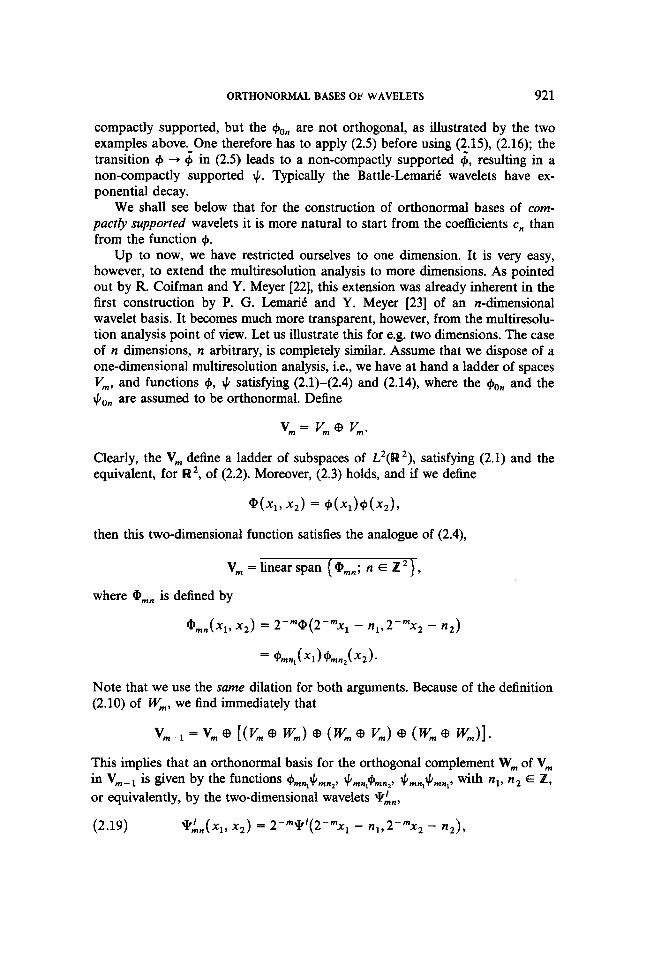
Up to now, we have restricted ourselves to one dimension. It is very easy, however, to extend the multiresolution analysis to more dimensions. As pointed out by R. Coifman and Y. Meyer [22], this extension was already inherent in the first construction by P. G. LemariC and Y. Meyer [23] of an n-dimensional wavelet basis. It becomes much more transparent, however, from the multiresolu- tion analysis point of view. Let us illustrate this for e.g. two dimensions. The case of n dimensions, n arbitrary, is completely similar. Assume that we dispose of a one-dimensional multiresolution analysis, ie., we have at hand a ladder of spaces V,, and functions +, + satisfying (2.1)-(2.4) and (2.14), where the and the +on are assumed to be orthonormal. Define
v,= V,@ V,.
Clearly, the V, define a ladder of subspaces of Lz(R2) , satisfying (2.1) and the equivalent, for W z , of (2.2). Moreover, (2.3) holds, and if we define
W X l , x2) = +(X l )+ (XZL
then this two-dimensional function satisfies the analogue of (2.4),
v,,, = linear span { Q,~; n E z *}, where a,, is defined by
Qmn(X1, x 2 ) = 2-"Q(2-"x1 - n1,2-mx2 - n 2 )
= +mn, ( x1) +mn, ( x2 ).
Note that we use the same dilation for both arguments. Because of the definition (2.10) of W,, we find immediately that
V m - 1 = v m @ [ ( V m @ w m ) 0 ( w m @ Vm) ( w m @ w m ) l .
This implies that an orthonormal basis for the orthogonal complement W, of V, in V,-I is given by the functions +,,,n,+mn,, +,,,+m,,, + m n , + m q ~ with n1, n2 E E, or equivalently, by the two-dimensional wavelets *A,, (2.19) +An(x1, x2) = 2-m\k'(2-mx1 - nl ,2-"x , - n 2 ) ,
922 I. DAUBECHIES
where 1 = 1,2,3, n E Z2, and
(2.20)
(2.22)
It follows that the *La, 1 = 1,2,3, m E Z, n E Z 2, constitute an orthonormal basis of wavelets for L2(W2).
The above construction shows how any multiresolution analysis + associated wavelet basis in one dimension can be extended to d dimensions. The decomposi- tion + reconstruction algorithm constructed by S . Mallat for visual data in [8] uses such a two-dimensional basis.
2.B. The Laplacian pyramid scheme of P. Burt and E. Adelson. In this subsection we review some aspects, relevant for the present paper, of Burt and Adelson's algorithm for the decomposition and reconstruction of images. For a more detailed presentation, and for applications, we refer the reader to [20].
One of the goals of a decomposition scheme for images is to remove the very high correlations existing between neighboring pixels, in order to achieve data compression. Several different schemes have been proposed to achieve this. Typically they use a prediction method, in which the value at a pixel is predicted (by a weighted average) from either previously encoded or neighboring pixels, and only the difference between the actual pixel value and the predicted value is encoded. Using the neighboring pixels for prediction is more natural and should lead to more accurate prediction (and therefore to greater data compression), but is much harder to implement than the easy causal prediction scheme, using only previously encoded pixels. The scheme proposed by Burt and Adelson combines the ease of computation of a causal scheme with the advantages and elegance of a neighborhood-based (noncausal) scheme. The result is-we quote directly from [2Oa]-
" . . - a technique for image encoding in which local operators of many scales but identical shape serve as the basis functions."
The analogy with multiresolution analysis is evident from this quote. Images are two-dimensional, and the Laplacian pyramid scheme is a two-
dimensional algorithm. For simplicity, the review below will be restricted to one dimension. This does not really matter, except in details (which will be pointed out). Moreover, the two-dimensional schemes used in [20] are in fact obtained (for simplicity reasons) as a tensor product of two one-dimensional schemes.
Our presentation will be already adapted to later use in this paper, and slightly different in notation from [20]. Except for this difference, what follows is the construction in [20].
ORTHONORMAL BASES OF WAVELETS 923
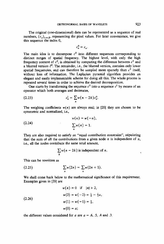
The original (one-dimensional) data can be represented as a sequence of real numbers, ( c , , ) , , ~ ~ , representing the pixel values. For later convenience, we give this sequence the index 0,
c," = c,.
The main idea is to decompose co into different sequences corresponding to distinct ranges of spatial frequency. The highest level, with only the high frequency content of co, is obtained by computing the difference between co and a blurred version Fo. The remainder, i.e., the blurred version, contains only lower spatial frequencies, and can therefore be sampled more sparsely than co itself, without loss of information. The Laplacian pyramid algorithm provides an elegant and easily implementable scheme for doing all this. The whole process is repeated several times in order to achieve the desired decomposition.
One starts by transforming the sequence co into a sequence c1 by means of an operator which both averages and decimates,
(2 .23) c: = C w ( n - 2k)c,". n
The weighing coefficients w ( n ) are always real; in [20] they are chosen to be symmetric and normalized, i.e.,
(2.24) w ( n ) = w ( - n ) ,
C w ( n ) = 1 . n
They are also required to satisfy an "equal contribution constraint", stipulating that the sum of all the contributions from a given node n is independent of n, i.e., all the nodes contribute the same total amount,
w ( n - 2 k ) is independent of n . k
This can be rewritten as
(2.25) C w ( 2 n ) = C w ( 2 n + 1 ) . n n
We shall come back below to the mathematical significance of this requirement. Examples given in [20] are
w ( n ) = 0 if In1 > 2,
(2 .26) w ( 2 ) = w ( - 2 ) = a - fa, w ( 1 ) = w ( - 1 ) = a, w ( 0 ) = a ;
the different values considered for a are CI = .6, .5, .4 and .3.
924 I. DAUBECHIES
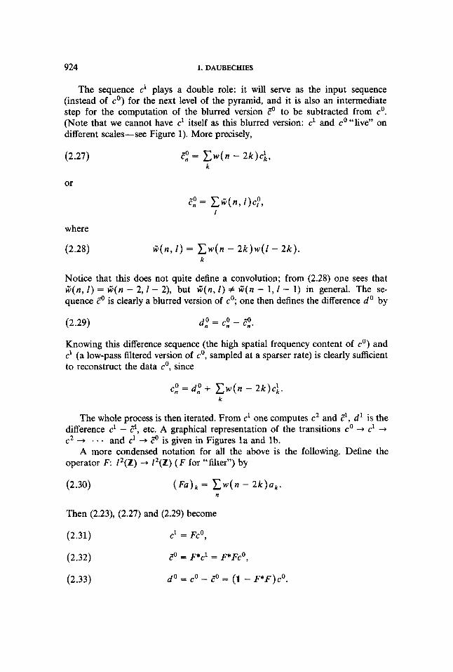
The sequence c1 plays a double role: it will serve as the input sequence (instead of co) for the next level of the pyramid, and it is also an intermediate step for the computation of the blurred version to be subtracted from co. (Note that we cannot have c1 itself as this blurred version: c1 and live" on different scales-see Figure 1). More precisely,
(2.27) = C w ( n - 2 k ) c k , k
where
(2.28) q n , I ) = C w ( n - 2k)w(Z - 2 k ) . k
Notice that this does not quite define a convolution; from (2.28) one sees that G(n, I ) = G ( n - 2 , I - 2), but G ( n , I ) # E(n - 1, I - 1) in general. The se- quence C'O is clearly a blurred version of co; one then defines the difference d o by
d t = c," - -0 (2.29) c n -
Knowing this difference sequence (the high spatial frequency content of co) and c1 (a low-pass filtered version of co, sampled at a sparser rate) is clearly sufficient to reconstruct the data co, since
c," = d,O + C W ( ~ - 2 k ) ~ k . k
The whole process is then iterated. From c1 one computes c2 and Z1, d1 is the difference c1 - El , etc. A graphical representation of the transitions co + c1 +
c2 + . - A more condensed notation for all the above is the following. Define the
operator F 12(Z) -+ 12(Z) ( F for "filter") by
and c1 + C"O is given in Figures l a and lb.
(2 .30) ( F a ) k = C W ( ~ - 2 k ) a k . n
Then (2.23), (2.27) and (2.29) become
(2 .31) c1 = Fc0,
(2.32) ,? = p c 1 = F*F~O,
(2.33) d o = co - Eo = (1 - F*F)c0 .
ORTHONORMAL. BASES OF WAVELETS 925
cl,
Figure 1. Graphical representation of the Laplacian pyramid scheme (redrawn from [203).
w(n) = 0 if JnJ > 2, and only the computation of r$, and ci are depicted. a. The transition co + 2 -B cz. For simplicity's sake we have restricted ourselves to the case
b. The transition c' -B 9.
Here we use the standard notation F* for the adjoint of the (bounded) operator F. Note that we implicitly assume that co E 12(Z), or, in signal analysis terms, that the data sequence co has finite energy. In practice, the sequence co is finite, and this constraint does not matter.
The total decomposition consists thus in L consecutive steps (in practice L = 5 or 6), with
From the sequences d o , . - ., dL- l , c L one then reconstructs co recursively by
At every step, in the decomposition (2.34) as well as in the reconstruction (2.35) the same filter coefficients are used, and all the operations involved are direct and linear (no solving of complicated systems of equations!). This makes
926 I. DAUBECHIES
this algorithm very easy to implement. The decimation aspect in the operator F, which reduces the number of entries in the c‘ by a factor 2 at every step, makes the whole decomposition algorithm as fast as a fast Fourier transform (see [20]).
Let N be the total number of non-zero entries in co. Then the total number of entries in d o , . - -, d L - l , c L (except for edge effects) is
N + N / 2 + * * * + N / 2 L - 1 + N / 2 L = 2N(1 - 2 - L - ’ ) .
After the Laplacian pyramid decomposition there is thus a larger number of entries (almost twice as many) than in the original data sequence. However, it turns out that, because of the removal of correlations, the decomposed data can be greatly compressed (see [2Oa]). The net effect is still an appreciable data compression. We shall not go into this here, however. Note that the increase of the number of entries is less pronounced in two dimensions (a factor 4 instead of
The similarity between the Laplacian pyramid algorithm and a multiresolu- tion analysis is now clear. In both approaches, the data (a function in multireso- lution analysis, a sequence in the Laplacian pyramid) are decomposed into a “ pyramid” of approximations, corresponding to less and less detail. Moreover, the differences between each two successive approximations are computed (corre- sponding to the wavelet decomposition in the multiresolution analysis). However, it is also clear that the schemes are quite different in the details of the computa- tion of the decomposition. The algorithm developed by S. Mallat, described in the next subsection, retains the attractive features of the Laplacian pyramid scheme, but is much closer to the analysis described in subsection 2 A .
The filter coefficients w(n) , or equivalently the filter operator F, are associ- ated in [20] with “equivalent weighting functions”. Only the limit of these functions will be relevant for us; we conclude this subsection by its definition and a few of its properties. One may wonder which kind of input sequence co corresponds to the “simplest” decomposition sequence, i.e., to d o = - . - = dL-’ = 0, and ( c L ) , = an0. The answer is obviously (use the reconstruction algorithm)
2) .
0 - F * L ( 2 . 3 6 ) c -4 ) e ,
where e is the sequence e , = an0. If, e.g., L = 1, then the entries of co are exactly the w ( n ) . Since any sequence can be considered as a sum of translated versions of e , the sequence co = (F*)Le gives the basic building block for the subspace ( F*)L12(Z), i.e., for the L-th level component sequences. It is therefore important that these sequences co do not look messy, which they well might, for L large enough (for a “messy” example, see Figure 4 in subsection 3B). One can make a graphical representation of the co defined by (2.36), for successive L. We represent the sequence e by a simple histogram, with value 1 for - 5 5 x < &, 0 otherwise (see Figure 2). The sequence P e “lives” on a scale twice as small, and will therefore be represented by a histogram with step widths & (as opposed to 1 for e ) ; its different amplitudes are given by 2( F*e),, = 2w(n) . Similarly, (F*)‘e is
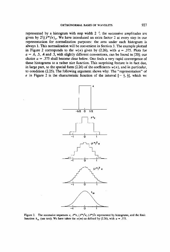
ORTHONORMAL BASES OF WAVELETS 927
represented by a histogram with step width 2-I; the successive amplitudes are given by 2‘((F*)‘e),. We have introduced an extra factor 2 at every step in our representation for normalization purposes: the area under each histogram is always 1. This normalization will be convenient in Section 3 . The example plotted in Figure 2 corresponds to the w ( n ) given by (2.26), with a = .375. Plots for a = .6, .5, .4 and .3, with slightly different conventions, can be found in [20]; our choice a = .375 shall become clear below. One finds a very rapid convergence of these histograms to a rather nice function. This surprising feature is in fact due, in large part, to the special form (2.26) of the coefficients w ( n ) , and in particular, to condition (2.25). The following argument shows why. The “representation” of e in Figure 2 is the characteristic function of the interval [ - 4, $[, which we
I l l -1/2 0 112
- 1 0 1
-1 0 1
(F*l3 e A -1 0 1
Figure 2. The successive sequences e, P e , ( P ) ’ e , (F*)3e represented by histograms, and the limit function h , (see text). We have taken the w ( m ) as defined by (2.26), with a = .375.
928 I. DAUBECHIES
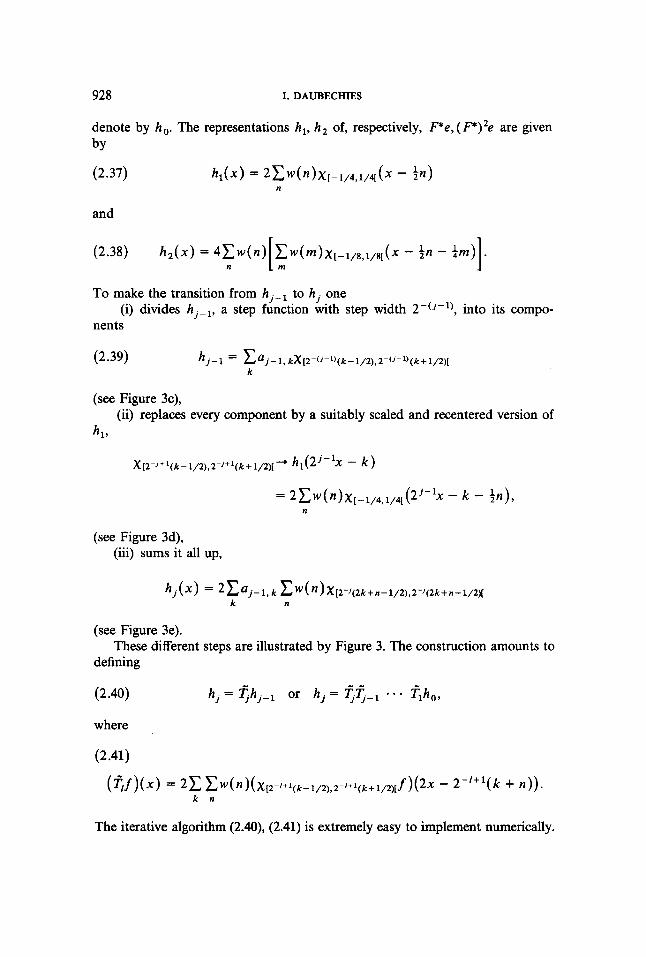
denote by ha. The representations h,, h2 of, respectively, FCe,(F*)2e are given by
(2.37) h l ( x ) = 2 C w ( n ) X [ - 1 / 4 , 1 / 4 [ ( X - in) n
and
To make the transition from h j - l to hi one
nents (i) divides h j P l , a step function with step width 2-('-'), into its compo-
(2.39)
(see Figure 3c), (ii) replaces every component by a suitably scaled and recentered version of
hl ,
X [ 2 - J + l ( k - 1 / 2 ) , 2 - ) + ' ( k + l / 2 ) [ -b h,(2j-'x - k )
= 2 C w ( " ) x [ - 1 / 4 , 1 / 4 [ ( 2 i - 1 x - - in), n
(see Figure 3d), (iii) sums it all up,
(see Figure 3e).
defining These different steps are illustrated by Figure 3. The construction amounts to
- - h . = f . h . or h i = T,.qp1 . . a f l h a , (2.40) J J J - 1
where
The iterative algorithm ( 2 4 , (2.41) is extremely easy to implement numerically.
ORTHONORMAL BASES OF WAVELETS 929
b) h j
w (-2 1 I
-1
d) I
i
e) h p
-1 0 1
e) h p
-1 0 1
Figure 3. a) h d x ) = x[-1/2,1/2[(x); b) h l ( x ) = ~~(n)~[n/~-1/4.n/~+1/41(~), c) h, is decomposed into its “components”; each component is a multiple of the characteristic
function of an interval of length $. (The “components” of hj would have width 2 - j ) .
d) Each “component” is replaced by a proportional version of h,, centered around the same point as the component, and scaled down by a factor $. (This scaling factor would be 2-J for hi).
e) The functions in d) are added to constitute h2 (or h,,,, if one starts from hi in c)).
930 I. DAUBECHIES
The h j can, however, also be written differently. Let us go back to expressions (2.36), (2.37) for h,, h2. These can be rewritten as
(2.42) h l ( x ) = 2 C w ( n ) h 0 ( 2 x - n ) , n
ORTHONORMAL BASES OF WAVELETS 931
Since (see (2.42), (2.43)) h, = Tho, h , = T2ho , it follows that
which proves (2.44). We have thus two different ways, (2.44) and (2.40), to compute the h,. Figure
2 shows that, at least for some choices of the w ( n ) , the functions h, converge, for j + 00, to a “nice” function h,. The explicit proofs which wi l l be given in subsection 3B show that, at least for the examples (2.26) with .125 < u < .625, the function h , is continuous (see (2.46) below), has compact support, and that the convergence h, + h , is uniform. Let us just accept these facts for the moment.
The two formulas (2.40) and (2.44) are both extremely useful in the study (and the proof) of this convergence. The construction of h , = lim,+,h, via (2.40) has the following nice localization feature. To compute the value of h +l(x) the recursion h,+l = q h , uses only values h , ( y ) for Iy - XI 5 2-J-*(N + l), where we assume w ( n ) = 0 for n 2 2N. Consequently, the val- ue of h , ( x ) can be computed using only the values of h , ( y ) for ly - XI 5 2-J(N + 1). For increasing j , this lends a “zoom-in“ quality to the graphical construction of which Figure 2 is an example. This is extremely useful when one wants to focus on details of the behavior of h , (see, e.g. Figure 6 in sub- section 4B). This localization feature is not present in (2.44). The formula h , ( x ) = (Th , - , ) (x ) uses values of hJ- l at points which stay at fixed distance of each other (i.e., 2x, 2(x f t ) , 2(x f l), . - ), independently of how large j is. The usefulness of (2.44) is therefore not “graphical”. It is, however, this less local formula which will be most useful in proving convergence of the h,, continuity of h,, etc.
Introducing Fourier transforms, (2.45) can be rewritten as
where
w([ ) = C w ( n ) e i n ‘ . n
Consequently, from (2.45), one obtains
sin( 2 - I - ‘ 4 ) A , ( [ ) = (2“)-1’2
932 I. DAUBECHIES
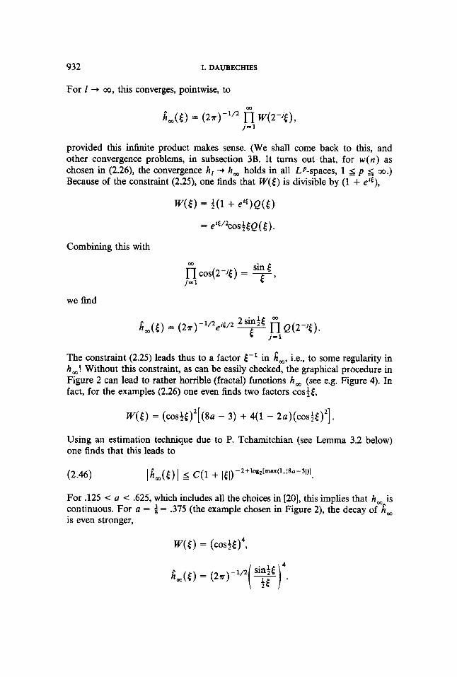
For 1 + 00, this converges, pointwise, to
m
j-1 im(() = (27r)-ll2 fl W ( 2 3 ) ,
provided this infinite product makes sense. (We shall come back to this, and other convergence problems, in subsection 3B. It turns out that, for w ( n ) as chosen in (2.26), the convergence h, -+ h , holds in all LP-spaces, 1 5 p ao.) Because of the constraint (2.25), one finds that W([) is divisible by (1 + e't),
Combining this with
Sin [ m
j-1
we find
The constraint (2.25) leads thus to a factor [-' in i,, i.e., to some regularity in h,! Without this constraint, as can be easily checked, the graphical procedure in Figure 2 can lead to rather horrible (fractal) functions h , (see e.g. Figure 4). In fact, for the examples (2.26) one even finds two factors cost[,
W ( t ) = ( C O S ~ ~ ) ~ [ ( ~ U - 3) + 4(1 - ~ U ) ( C O S ~ ~ ) ~ ] .
Using an estimation technique due to P. Tchamitchian (see Lemma 3.2 below) one finds that this leads to
For .125 c a c .625, which includes all the choices in [20], this implies that h,-is continuous. For a = = .375 (the example chosen in Figure 2), the decay of h , is even stronger,
ORTHONORMAL BASES OF WAVELETS 933
In this case, h, is thus a fourth-order convolution of xLo,l[ with itself, which results in a C3-‘ function.
The above remarks show that constraints on the w(n) , corresponding to divisibility of W(E) by (1 + ei6), result in regularity of h,. Constructions similar to (2.44) will be used in Section 3, where the above “trick” for imposing regularity on h , will turn up again.
This concludes our review of the Laplacian pyramid scheme. The above is by no means a complete review; only those aspects relevant to the present paper have been highhghted. For more details, and especially for applications (data compression, image splining) the reader should consult [20a] and [20b].
Remark. During the last revision of this paper before publication, Y. Meyer drew my attention to related work by G. Deslauriers and S . Dubuc [29]. They are interested in functions defined recursively by the following interpolation scheme. At the I-th step, the values of f at the points 2-‘(2k + l) , k E Z, are computed from the f ( k 2 - ‘ + I ) via the formula
In many applications considered by Deslauriers and Dubuc, the interpolation procedure is symmetric, i.e., a_, = a,,, for all m E Z. For suitable choices of the a,, the functions f constructed via this dyadic interpolation scheme, starting from the f( k), k E Z, are continuous, and are therefore completely characterized by their values at the dyadic rational points x = k2-‘, k E Z, I E N. A typical function f can be written as
where g is the function obtained by interpolation from g(0) = 1, g ( k ) = 0 for k E Z \ (0). The definition of g via the dyadic interpolation scheme is exactly the same as our “graphical recursion” (2.40), with the choice w(0) = t , w(2n) = 0 for n # 0, w(2n + 1) = +a,+,, n E Z. The analysis of the properties of g in [29] is then carried out by means of the same correspondence between “graphical recursion” and the iterative formula (2.44). Imposing Cam = 1 (i.e., C w ( n ) = 1) immediately leads to w ( < ) = [ $(l + e”)]’Q(<), which is then exploited, in [29], to impose continuity on g. There is therefore a clear similarity between the techniques used here and those exposed in [29]. The applications are different, however. Moreover, the proofs given in Section 3 apply to more general cases than those in [29], since we do not impose w(2n) = 0 for n # 0, nor w(2n + 1)
2.C. The wavelet based decomposition and reconstruction algorithm of S. Mallat. In [8], St6phane Mallat exploits the attractive features of multiresolu- tion analysis to construct a decomposition and reconstruction algorithm for
= w ( - 2 n - 1).
934 I. DAUBECHIES
2-d-images that has the same philosophy as the Laplacian pyramid scheme, but is more efficient and orientation selective. It is interesting to remark that the development of the concept of multiresolution analysis was triggered by the multiresolution methods, and in particular by the Laplacian pyramid. The full mathematical study of the concept, by S. Mallat and Y. Meyer, was done more or less simultaneously with the practical development, by S. Mallat, of his algorithm for vision analysis and reconstruction. This is not the only instance in which theoretical developments concerning wavelets find their inspiration in applica- tions: the last few years have seen a constant feedback between theory and applications. In fact, this paper is another such instance.
Let us start by a review of the algorithm in one dimension. As in the previous subsection, we want to decompose a sequence co = (ct), E 1*(2) into levels corresponding to different spatial frequency bands. To achieve this, we shall use a multiresolution analysis, which can be chosen freely (as long as (2.1)-(2.4) are satisfied), but has to be kept fixed for the whole algorithm. We suppose thus that we have chosen spaces V, and a function 4 such that (2.1)-(2.4) are satisfied. We assume (if necessary, we apply (2.5) first) that the @on are orthonormal. Let { +,,,”; rn, n E Z } be the associated orthonormal wavelet basis (we shall keep the same notations as in subsection 2A). The multiresolution analysis and orthonor- ma1 basis chosen in [8] is one in which the V, consist of cubic spline functions (cf. Examples 2.2 and 2.3, corresponding to linear and quadratic splines, respectively); the corresponding orthonormal basis is one of the Battle-LemariC bases. In what follows we shall assume that both 4 and t) are real, as they are in [8] and indeed in most practical examples.
Form the data sequence co E /’(if) we construct a function f ,
f = C C k o n , n
or
This function is clearly an element of V,. We can now use the whole multiresolu- tion analysis apparatus on this function. We shall compute the successive Pj f , corresponding to more and more “blurred” versions of f (and hence of the data sequence co), and also the Q , f , corresponding to the difference in information between the “versions” of f at two successive resolution levels. Eventually, of course, this has to be translated back to a “sequence” (as opposed to a “function”) language, but this turns out to be very easy.
As element of Yo = Vl @ W,, f can be decomposed into its components along V, and W,,
f = pif + Q i f .
ORTHONORMAL. BASES OF WAVELETS 935
Each of these components can be expanded with respect to the orthonormal bases itln, respectively,
The sequence c1 represents a smoothed version of the original data sequence coy while dl represents the difference in information between co and c1 (cf. the discussion of pi, Q, in subsection 2A). The sequences cl, di can be computed as a function of co in the following way. Since the are orthonormal bases of V,, one has
where
= 2-'/2/dx+(:x)c#I(x - (n - 2k)).
This can be rewritten as
(2.47)
with
c: = C h ( n - 2k)c,0 n
h ( n ) = 2-'/2jdx+('ix)$J(x - n).
Note that these h ( n ) are, up to a normalization factor 2-'12, exactly the coefficients c ( n ) appearing in (2.15). Similarly,
(2.48)
with
d; = C g ( n - 2k)cH n
g ( n ) = 2-'/2/dx+(!x)+(x - n).
936 I. DAUBECHIES
It follows that the expressions for cl, d’ as a function of co are of exactly the same type as (2.23) in the Laplacian pyramid scheme. The main difference between the two schemes is that both the blurred, lower resolution c’ and the “difference” sequence d 1 are now obtained via a filter of type (2.23). The filter coefficients h ( n ) , g(n) are fixed by the chosen multiresolution analysis frame- work. It turns out that the h ( n ) have many properties in common with the w ( n ) in subsection 2B; for instance, the h( n) satisfy a normalization condition, i.e., C,h(n) = (see subsection 3A for an explanation of the difference in normal- ization with the w(n) ) . The requirement Cnh(2n) = C,h(2n + 1) is also satisfied by most interesting examples, and in particular in [8] (we shall come back to this later). The filter coefficients g ( n ) are of a different nature, as one would expect; in particular, C , g ( n ) = 0.
Introducing a shorthand notation similar to (2.30), we rewrite (2.47), (2.48) as
c’ = Hco,
d’ = Gco,
where H, G are bounded operators from 12(Z) to itself,
(2.49)
The procedure can now be iterated; since P, f E V, = V2 @ W2, we have
One finds then
It is very easy to check, however, that
ORTHONORMAL BASES OF WAVELETS 937
independently of j . It follows that
or
c2 = Hc'. Similarly,
d 2 = Gc'
Clearly this can now be iterated as many times as wanted. At every step one finds
p, - i f = P,f -k Q J f
= C C b J k + C d i $ J k k k
with
(2 .50) cJ = HcJ-1,
(2.51) d J = GcJ-1.
This is the desired decomposition. The successive cJ are lower and lower resolution versions of the original co, each sampled twice as sparsely as their predecessor (due to the factor 2 in the filter coefficients in (2.47)), and the d J contain the difference in information between cJ-' and cJ. Moreover, the cJ, d J are computed via a tree algorithm (2.50), (2.51). This computation is therefore as easy to implement as the Laplacian pyramid scheme.
Note that Mallat's algorithm is more economical than the Laplacian pyramid scheme. In practice, one will again stop the decomposition after a finite number L of steps, i.e., co will be decomposed into d',. - -, d L and cL. If co has initially N non-zero entries, then (neglecting edge effects) the total number of non- zero entries in the decomposition is N / 2 + N / 4 + e - . + N/2L-' + N / 2 L + N / 2 L = N . This shows that, unlike the Laplacian pyramid scheme (see subsec- tion 2B), Mallat's algorithm preserves, at every step, the number of non-zero entries (as was to be expected from an algorithm based on an orthonormal basis decomposition).
So far we have only described the decomposition part of the algorithm. The reconstruction part is just as easy. Suppose we know cJ and dJ. Then
k k
938 I. DAUBECHIES
and hence
= z h ( n - 2k)ci + z g ( m - 2k)d;C‘, k k
or
(2.52) C J - 1 = H*cJ + G*dJ.
The reconstruction algorithm is therefore also a tree algorithm, using the same filter coefficients as the decomposition.
Remark. In fact, the transition cj- ’ 4 c j , d J corresponds to a change of basis in V’-’, {+,-1k; k E Z} + { +jk, #,k; k E E ) . Because of the underlying wavelet structure the orthogonal matrix associated to this basis change has a peculiar structure. The transition cJ, d J + c j - l is given by the transposed matrix; this is the reason why the adjoints H*, G* of H and G turn up in (2.52).
All the above is one-dimensional. As an image decomposition-and reconstruc- tion algorithm, Mallat’s scheme is of course two-dimensional, and corresponds to a two-dimensional multiresolution analysis (see subsection 2A). Since the corre- sponding wavelet basis vectors can all be written as products of one-dimensional #,k, +jpjk (see (2.19)-(2.22)), the two-dimensional algorithm itself can also be generated by a “ tensor product” of the one-dimensional algorithm (see [S]). More specifically, the sequences to be decomposed are now elements of Z2(Z2),
and one defines G,, H, and G,, H, as the filters G , H defined by (2.49), but acting only on the first, respectively, the second, coefficient ( r for “rows”, c for “columns”). Then co is decomposed into c1 and three difference sequences (corresponding to the \ k j , j = 1,2,3,-see (2.20)-(2.22)) d l* l , d’,’ and d1v3,
c1 = H ~ H , C O ,
d’,’ = GcH,co,
d1I2 = HCGrco,
d1y3 = G , G ~ c O .
The operator G,Hr “smooths” over the column index, and looks at the “dif- ference” (+ high frequency information) for the row index; typically, d’.’ will
ORTHONORMAL BASES OF WAVELETS 939
be large when a horizontal edge is present. Similarly, d1,2 detects vertical edges. It follows that, at no extra cost, Mallat’s algorithm is orientation sensitive, which the two-dimensional Laplacian pyramid scheme of [20] was not. In [8], S. Mallat gives a very striking graphical representation of the whole two-dimensional scheme, illustrated with several examples, which clearly show, in particular, the orientation specificity of his algorithm.
3. Equivalence Between Mallat’s Discrete Algorithm and Multiresolution Analysis
3.A. Weaning Mallat’s algorithm from its multiresolution parent. Ulti- mately, Mallat’s decomposition and reconstruction algorithm, i.e., (2.50), (2.51) and (2.52), deals only with sequences; the underlying multiresolution analysis is only used in the computation of the filter operators H and G. In this subsection we extract the properties of H and G that make the scheme work, without reference to multiresolution analysis.
These properties are very easy to deduce from subsection 2C. First of all, we impose
c IW I < 00,
Clg(n) l < 00.
(3.1) n
n
This implies that the operators H, G, defined by
( H a ) , = c h ( n - 2k)an, n
( G a ) , = c S ( n - 2k)a,,
are bounded operators on Z2(Z). This condition is satisfied by the h ( n ) , g ( n ) in subsection 2 C ; it corresponds to a rather weak decay condition on (p. At later stages, we shall impose much stronger decay conditions on the h ( n ) .
A second condition follows from the decomposition formulas (2.50), (2.51) and the reconstruction formula (2.52). The scheme will only work if
(3.2)
splits the original 12(Z) into a sum of subspaces. After the first step, we have
n
H*H + G*G = 1.
The third condition expresses orthogonality. Essentially, the decomposition
1 2 ( Z ) = H*12(Z) 8 G * I Z ( Z ) ;
after L iterations, one finds L-1
j - 0 1 2 ( Z ) = @ (H*)’G*12(Z) + ( H * ) L I Z ( Z ) .
940 I. DAUBECHIES
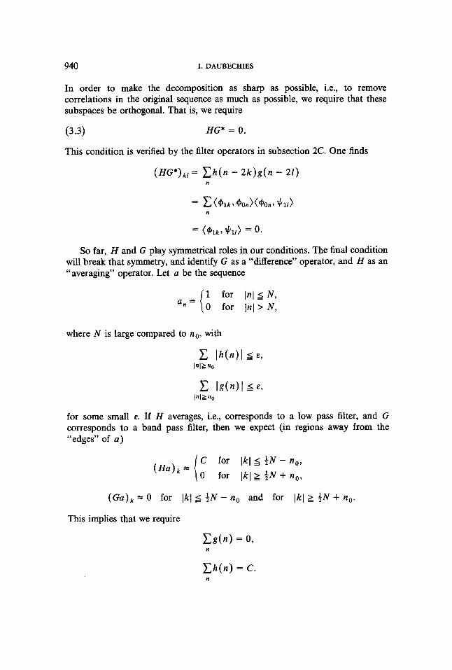
In order to make the decomposition as sharp as possible, i.e., to remove correlations in the original sequence as much as possible, we require that these subspaces be orthogonal. That is, we require
(3.3) HG* = 0.
This condition is verified by the filter operators in subsection 2C. One finds
So far, H and G play symmetrical roles in our conditions. The final condition will break that symmetry, and identify G as a “difference” operator, and H as an “averaging” operator. Let a be the sequence
where N is large compared to no, with
for some small E. If H averages, i.e., corresponds to a low pass filter, and G corresponds to a band pass filter, then we expect (in regions away from the “edges” of a )
( G a ) , = 0 for Ikl 6 4N - no and for Ikl 2 i N + n o .
This implies that we require
C h ( n ) = c. n
ORTHONORMAL BASES OF WAVELETS 941
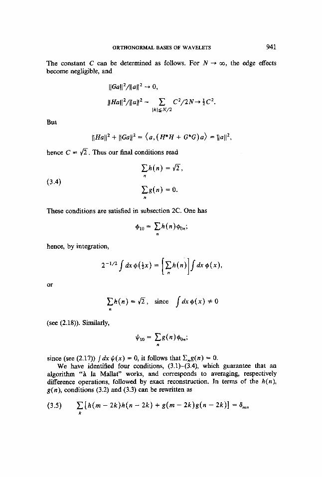
The constant C can be determined as follows. For N + 00, the edge effects become negligible, and
But
hence C = a. Thus our h a l conditions read
C h ( n ) = Ji, n
(3.4)
These conditions are satisfied in subsection 2C. One has
hence, by integration,
or
(see (2.18)). Similarly,
since (see (2.17)) j d x + ( x ) = 0, it follows that C n g ( n ) = 0. We have identified four conditions, (3.1)-(3.4), which guarantee that an
algorithm ‘‘A la Mallat” works, and corresponds to averaging, respectively difference operations, followed by exact reconstruction. In terms of the h ( n ) , g ( n ) , conditions (3.2) and (3.3) can be rewritten as
(3.5) C [ h ( m - 2k)h(n - 2 k ) + g(m - 2k)g(n - 2k)] = S,, k
942 I. DAUBECHIES
and
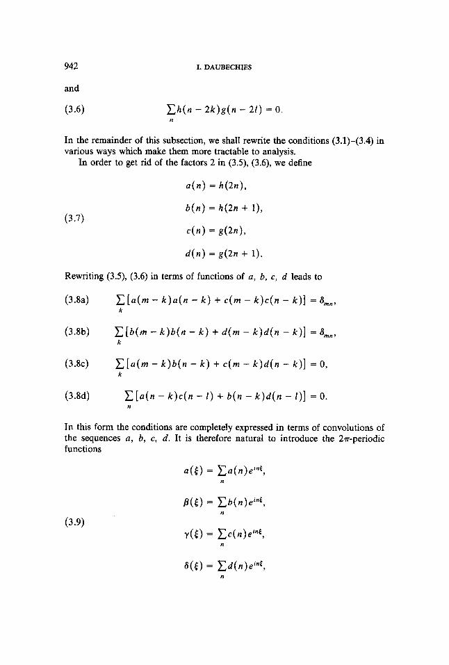
C h ( n - 2 k ) g ( n - 21) = 0. n
In the remainder of this subsection, we shall rewrite the conditions (3.1)-(3.4) in various ways which make them more tractable to analysis.
In order to get rid of the factors 2 in (3.5), (3.6), we define
a(.) = h ( 2 n ) ,
b ( n ) = h(2n + l), (3.7)
d(n) = g ( 2 n + 1).
Rewriting (3.5), (3.6) in terms of functions of a, b, c, d leads to
(3.8a) c [ u ( m - k ) a ( n - k) + c ( m - k ) c ( n - k ) ] = a,,, k
(3.8b) c [ b ( m - k ) b ( n - k) + d ( m - k ) d ( n - k ) ] = a,,, k
(3 .8~) C [ U ( ~ - k ) b ( n - k ) + ~ ( m - k ) d ( n - k)] = 0, k
(3.8d) C [ a ( n - k ) c ( n - I) + b ( n - k ) d ( n - I)] = 0. n
In this form the conditions are completely expressed in terms of convolutions of the sequences a, b, c, d. It is therefore natural to introduce the 27r-periodic functions
a ( ( ) = C a ( n ) e i n t , n
(3.9)
a([) = C d ( n ) e i n t , n
ORTHONORMAL BASES OF WAVELETS 943
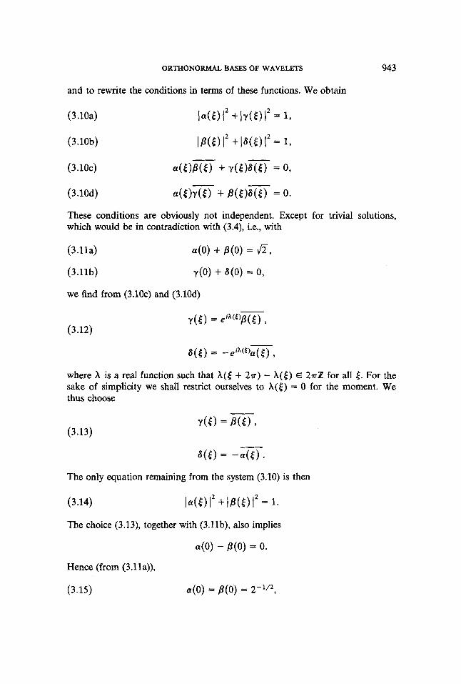
and to rewrite the conditions in terms of these functions. We obtain
These conditions are obviously not independent. Except for trivial solutions, which would be in contradiction with (3.4), i.e., with
(3.1 la)
(3.1 1 b)
a(0) + P ( 0 ) = a, Y(0) + W) = 0,
we find from (3.10~) and (3.10d)
(3.12)
a(() = -eiA(t)a(() ,
where X is a real function such that X ( l + 277) - A(() E 2 a Z for all E. For the sake of simplicity we shall restrict ourselves to A([) = 0 for the moment. We thus choose
(3.13)
The only equation remaining from the system (3.10) is then
The choice (3.13), together with (3.11b), also implies
a(O) - P ( O ) = 0.
Hence (from (3.11a)),
(3.15) a(O) = P(O) = 2-1/2,
944 I. DAUBECHIES
which agrees with (3.14) for [ = 0. It follows that any choice of 27-periodic functions a and P satisfying (3.14), (3.15) and Clanl < 00, Cn(bn( < 00, leads, via (3.13), (3.9) and (3.7), to two filter operators H and G satisfying (3.1)-(3.4). These filter operators can then be used for a decomposition and reconstruction algorithm ''A la Mallat", without reference to multiresolution analysis.
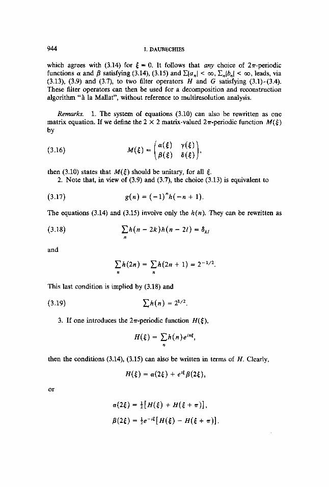
Remarks. 1. The system of equations (3.10) can also be rewritten as one matrix equation. If we define the 2 X 2 matrix-valued 27r-periodic function M( 5 ) by
(3.16)
then (3.10) states that M ( [ ) should be unitary, for all 5. 2. Note that, in view of (3.9) and (3.7), the choice (3.13) is equivalent to
(3.17) g ( n ) = ( - l ) " h ( - n + 1).
The equations (3.14) and (3.15) involve only the h(n) . They can be rewritten as
(3.18) C h ( n - 2 k ) h ( n - 21) = S,, n
and
C h ( 2 n ) = Ch(2n + 1) = 2-l/* n n
This last condition is implied by (3.18) and
(3.19) C h ( n ) = 2lI2
3. If one introduces the 27r-periodic function H ( [ ) ,
H ( [ ) = C h ( n ) e t n t , n
then the conditions (3.14), (3.15) can als6 be written in terms of H. Clearly,
H ( 0 = 4 0 + e'EP(20,
or
ORTHONORMAL BASES OF WAVELETS 945
Then (3.14), (3.15) are equivalent with
(3.20)
and
(3.21) H ( 0 ) = a. Under the form (3.20) this condition is not new. It can be found in [16], where mo([) = 2-'/'H(5) is used, rather than H. While this paper was being written, S. Mallat pointed out to me that (3.20) is very similar to a condition derived by M. Smith and T. Barnwell [24] in the construction of "conjugate quadrature filters". In fact, (3.20) is identical to their condition. Smith and Barnwell were looking for, and found, a tree-structured two-band coding scheme with exact reconstruction, which is exactly what this subsection is about! The constructions given later (at least insofar as they describe discrete filters) are therefore, in fact, special cases of their construction. Ultimately, however, our aim here is to construct orthonormal wavelet bases of compact support, which is a very differ- ent point of view. Even from the filter point of view, our results go further than Smith and Barnwell's, in that we give complete characterization of the possible filters. We shall however not go into this here.
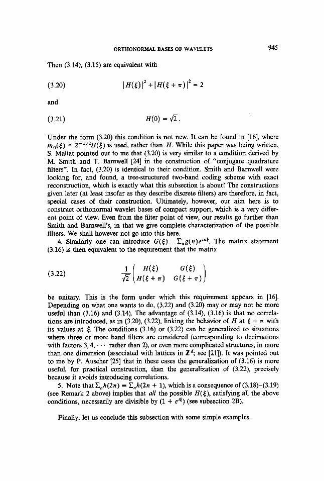
4. Similarly one can introduce G ( 5 ) = E,g(n)e'"€. The matrix statement (3.16) is then equivalent to the requirement that the matrix
(3.22)
be unitary. This is the form under which this requirement appears in [16]. Depending on what one wants to do, (3.22) and (3.20) may or may not be more useful than (3.16) and (3.14). The advantage of (3.14), (3.16) is that no correla- tions are introduced, as in (3.20), (3.22), linking the behavior of H at 5 + 7r with its values at E. The conditions (3.16) or (3.22) can be generalized to situations where three or more band filters are considered (corresponding to decimations with factors 3,4, * * rather than 2), or even more complicated structures, in more than one dimension (associated with lattices in Zd; see [21]). It was pointed out to me by P. Auscher [25] that in these cases the generalization of (3.16) is more useful, for practical construction, than the generalization of (3.22), precisely because it avoids introducing correlations.
5. Note that C,h(2n) = Z,h(2n + l), which is a consequence of (3.18)-(3.19) (see Remark 2 above) implies that all the possible H ( t ) , satisfying all the above conditions, necessarily are divisible by (1 + e Y ) (see subsection 2B).
Finally, let us conclude this subsection with some simple examples.
946 I. DAUBECHIES
EXAMPLE 3.1. The simplest possible example is
a ( ( ) = P ( ( ) = 2-112,
corresponding to
h(0 ) = 2-112, g ( 0 ) = 2-112,
h ( 1 ) = 2-112, g ( 1 ) = -2-112,
all the other h( n ) , g( n ) being zero.
EXAMPLE 3.2. The next simplest example is
where v is an arbitrary real number, This corresponds to
h ( 0 ) = 2- ' /2v (v - 1 ) / ( v 2 + l), g(0) = 2- ' /2v(v + 1 ) / ( v 2 + l), h(1 ) = 2-'/2(1 - v ) / ( v ' + l), g(1) = - 2 - y v + 1 ) / ( v 2 + l), h ( 2 ) = 2 - y v + l ) / ( v 2 + l), g ( 2 ) = 2-'/*(1 - v ) / ( v ' + l),
h ( 3 ) = 2- ' /2v (v + 1)/(v2 + l ) , g ( 3 ) = -2 -1 /2v (v - l ) / ( v 2 + l ) ,
all the other h ( n ) , g ( n ) being zero.
Note. We have here taken
g ( n ) = ( - l ) " h ( 3 - n)
rather than (3.17); this shift corresponds simply to choosing A(() = ( instead of 0 in (3.12).
3.B. Introducing a regularity condition. In the preceding subsection we derived and discussed a set of necessary and sufficient conditions, directly on the filter operators, for Mallat's algorithm to work. All these conditions concerned only what happened in one step of decomposition/reconstruction. In the discus- sion, in subsection 2B, of the Laplacian pyramid scheme, we saw that it is also important that the iterated reconstruction, applied to a sequence consisting of only one non-zero entry, looks still reasonably nice, even after several iterations.
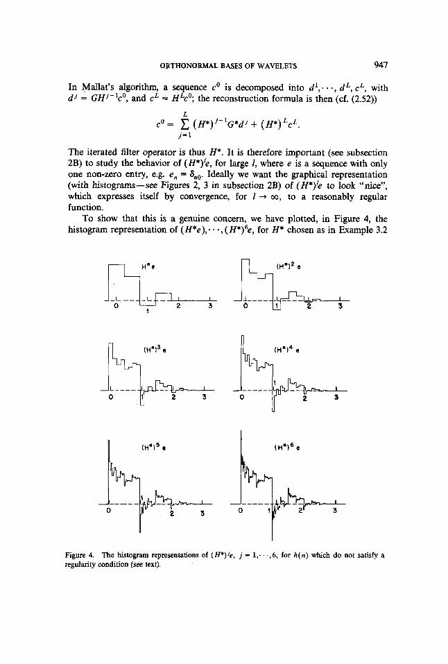
ORTHONORMAL BASES OF WAVELETS 947
In Mallat’s algorithm, a sequence co is decomposed into d’ , . . -, d L , cL, with d J = GHj-lc’, and c L = HLc0; the reconstruction formula is then (cf. (2.52))
L c0 = (H*)’-lG*d’ + ( H * ) L ~ L .
j - 1
The iterated filter operator is thus H*. It is therefore important (see subsection 2B) to study the behavior of (H*)‘e, for large 1, where e is a sequence with only one non-zero entry, e.g. en = an0. Ideally we want the graphical representation (with histograms-see Figures 2, 3 in subsection 2B) of (H*)’e to look “nice”, which expresses itself by convergence, for 1 + 00, to a reasonably regular function.
To show that this is a genuine concern, we have plotted, in Figure 4, the histogram representation of ( H * e ) , . - -, (H*)6e, for H* chosen as in Example 3.2
L I’Y
Figure 4. The histogram representations of (H*) j e , j = 1,. . . ,6 , for h ( n ) which do not satisfy a regularity condition (see text).
948 I . DAUBECHIES
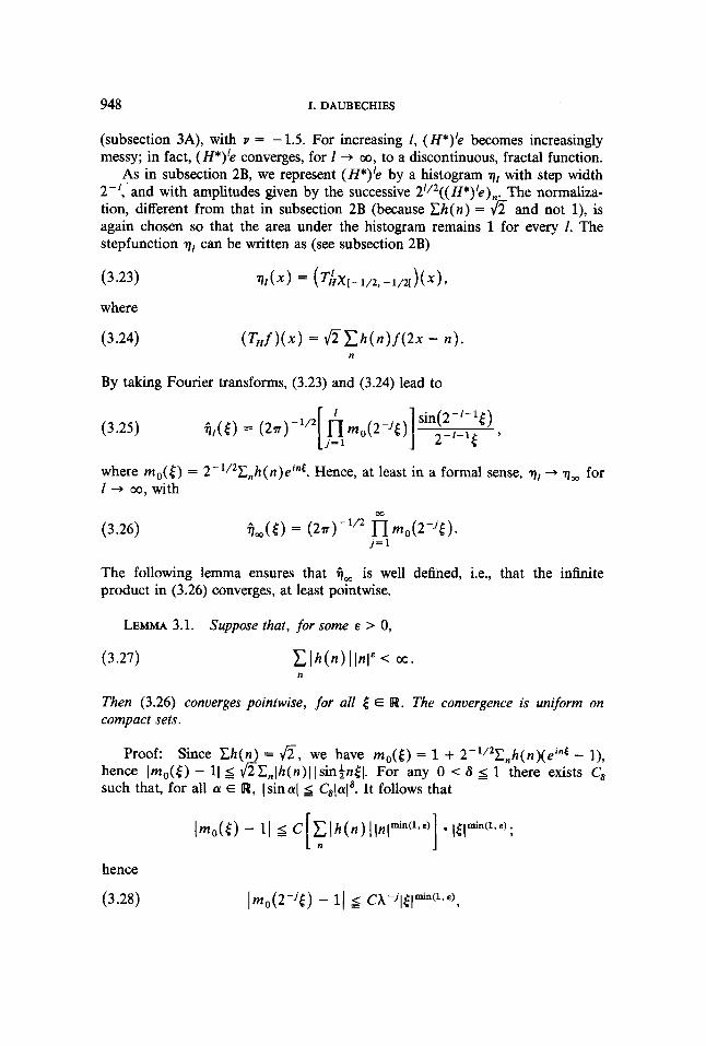
(subsection 3A), with v = -1.5. For increasing 1, (H*)'e becomes increasingly messy; in fact, (H*)'e converges, for I + 00, to a discontinuous, fractal function.
As in subsection 2B, we represent (H*)'e by a histogram qr with step width 2-', and with amplitudes given by the successive 2'/2((H*)'e)n. The normaliza- tion, different from that in subsection 2B (because C h ( n ) = fi and not l), is again chosen so that the area under the histogram remains 1 for every 1. The stepfunction can be written as (see subsection 2B)
(3.23) V / ( X ) = ( G X [ - 1 / 2 , -1/2[)(X),
where
(3.24) (THf )(.) = f i C h ( n ) f ( 2 x - 4. n
By taking Fourier transforms, (3.23) and (3.24) lead to
where mo(() = 2-1/2Cnh(n)eint. Hence, at least in a formal sense, q, + qm for I --f 00, with
(3.26)
The following lemma ensures that ijm is well defined, i.e., that the infinite product in (3.26) converges, at least pointwise.
LEMMA 3.1. Suppose that, for some E > 0,
(3.27)
Then (3.26) converges pointwise, for all 6 E W. The convergence is uniform on compact sets.
Proof: Since C h ( n ) = fi, we have m o ( t ) = 1 + 2-1/2Cnh(n)(e'nt - l), hence Imo(t) - 11 g aC, lh(n) l Isinfntl. For any 0 < S g 1 there exists C, such that, for all a E W, (sinal 5 C,lal'. It follows that
hence
(3.28)
ORTHONORMAL BASES OF WAVELETS 949
where X = 2rmn(1, > 1. This is sufficient to ensure convergence of (3.26), for any ( E W. It immediately follows from (3.28) that the convergence is uniform on compact sets.
Remark. While being more restrictive than (3.1), the condition (3.27) is still very mild. In practice one requires much stronger decay for the h(n) . For filter construction purposes, one even restricts oneself to the case where only finitely many h(n) are different from zero.
It is however not sufficient to know that 9, is well defined. In order to avoid situations such as depicted in Figure 4, we require that (i) 4, has sufficient decay, so that r ] , is sufficiently regular (at least continuous), and (ii) r] , converges to r],, pointwise, for 1 -, 00.
+ 00, of $,((), we shall use the same trick as in subsection 2B, i.e., we shall require that m o ( ( ) is divisible by (1 + eit)N, for some N > 0. The precise statement is given in the following lemma, using an estimation technique of P. Tchamitchian [S].
To ensure the decay, for
LEMMA 3.2. I f m o ( ( ) = (1 + e i t ) l N F ( ( ) , where*(() = C,f(n)e'"tsatisJies
(3.29) C l f ( n ) l I n l E < 00 forsome E > O
and
(3.30)
then there exists C > 0 such that, for all ( E W,
Remarks.
2. The condition (3.29) will automatically be satisfied if
1. It follows from (3.31) that r ] , is continuous if H satisfies all the above conditions, and if B < 2N-'.
(3.32)
950 I. DAUBECHIES
Proof: Since II~~,cos(2-jx) = x-’sin x, we have
W r m
where the right-hand side converges uniformly on compact sets because of (3.29). There exists therefore a constant C such that, for all 161 4 1,
(3.34)
Take now 161 > 1. Determine jo E N such that
(3.35) w ,
To estimate I17-1.F(2-j2-’o[) we have used the same argument as in the proof of Lemma 3.1. This is allowed since C f ( n ) =.F(O) = mo(0) = 1. Together, (3.35), (3.34) and (3.33) imply (3.31).
In our search for “regularity” we have, so-far, only used one of the special conditions on the h ( n ) , derived in subsection 3A, namely (3.4), C , h ( n ) = 6. And even that has not played a critical role, since it was only used for normalization purposes, and we could have as easily normalized by any other constant which happened to be the sum of the h ( n ) . For our last step, the proof that the histograms q, converge pointwise to the continuous function qm (assum- ing B is not too large), we need an extra ingredient, namely Imo($)l 5 1. Since,
ORTHONORMAL BASES OF WAVELETS 951
however (see (3.20)), as a consequence of (3.2)-(3.3), lmo(( )J2 + lmo(( + . ) I 2 = 1, this condition is automatically fulfilled for h( n ) satisfying (3.18)-(3.19).
PROPOSITION 3.3. Define mo(5) = 2-1/2Cnh(n)einE, where the h ( n ) satisfy (3.18), (3.19). Suppose moreover that
with S(c) = C, f(n)e'"€ such that
(3.37) C l f ( n ) l I n l e < 00 forsome E > o
and
n
(3.38) sup IS(() I = B < 2N-'. EcR
Then the piecewise constant functions ql, defined recursively by
(3.39) = f i C h ( n h , - $ x - 4 , n
with
V O b ) = X[-1/2,1/2[(X)>
converge pointwise to the continuous function q , defined by
00
em([) = (27r)-1/2 n m0(2-j5) . j - 1
Proof 1. As an intermediate step, we prove p 1 -+ q,, pointwise, where the p / are defined in the same recursive way as the ql, but starting from a different initial function, i' -t,x, -1 j x _I 0,
p o ( x ) = 1 - x , O j X 6 1 , otherwise.
2. Taking Fourier transforms, we find
From Lemma 3.1 it follows that + ij,, uniformly on compact sets. This
952 I. DAUBECHIES
implies that, for all 6 > 0, and for all R > 0, we can find I, such that, for all f L I,,
On the other hand, Grn E L' since B < 2N-1. It follows that for all 6 > 0 there exists R such that
L1-convergence of $, to i,, which implies pointwise convergence of pI to qrn, will then follow if we can prove that, for all 6 > 0, there exist R and I, large enough, so that, for all 12 I,,
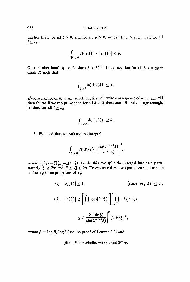
3. We need thus to evaluate the integral
where P I ( [ ) = lIf,,m0(2-j4). To do this, we split the integral into two parts, namely 5 2 ' ~ . To evaluate these two parts, we shall use the following three properties of PI:
2 2'77 and R 5
where p = log B/log2 (use the proof of Lemma 3.2) and
(iii) PI is periodic, with period 2'+'?r.
ORTHONORMAL BASES OF WAVELETS 953
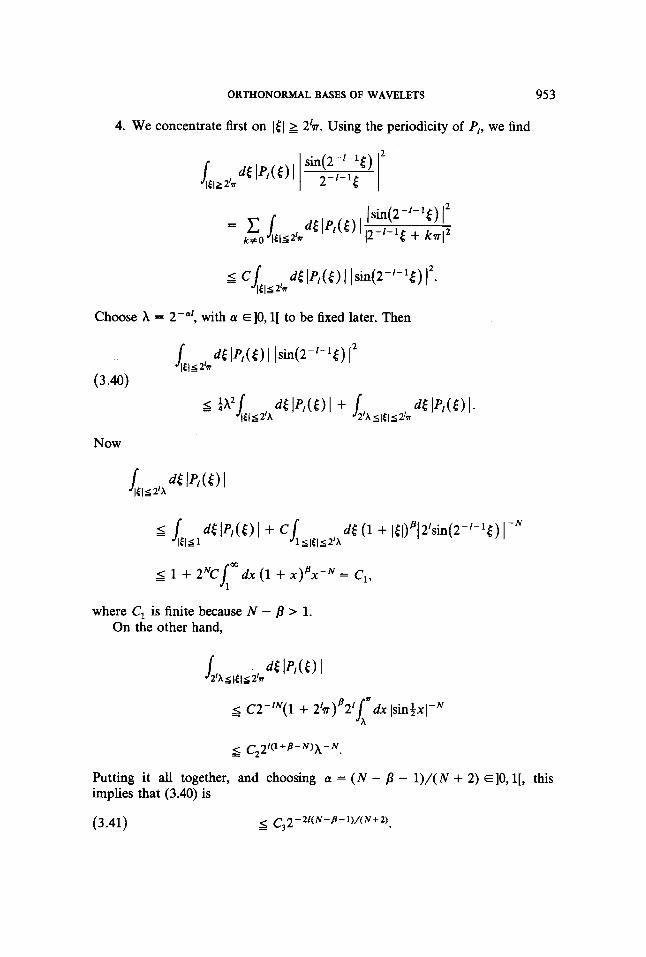
4. We concentrate first on 2 2b. Using the periodicity of P/, we find
Choose X = 2 - O ' , with a ~ ] 0 , 1 [ to be fixed later. Then
Now
where C, is finite because N - j3 > 1. On the other hand,
- - .= C22K1+B-N)h-N
Putting it all together, and choosing a = ( N - j3 - l)/(N + 2) ~ ] 0 , 1 [ , this implies that (3.40) is
(3.41) 5 c, 2 - W N - 8 - I)/( N+ 2)
954 I. DAUBECHIES
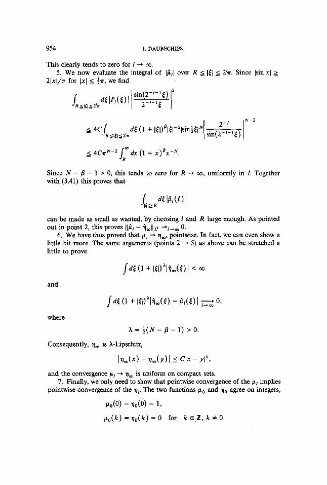
This clearly tends to zero for 1 --+ 00.
2(x(/n for 1x1 5 . We now evaluate the integral of I f i l l over R 141 5 2%. Since lsin XI 2
$71, we find
Since N - p - 1 > 0, this tends to zero for R + co, uniformly in 1. Together with (3.41) this proves that
can be made as small as wanted, by choosing 1 and R large enough. As pointed out in point 2, this proves llfil - i j m l l L 1 -'l-.W 0.
6. We have thus proved that pI + qm, pointwise. In fact, we can even show a little bit more. The same arguments (points 2 + 5 ) as above can be stretched a little to prove
J ~ E (1 + EDAI i jm(O I < 00
and
and the convergence pI + qm is uniform on compact sets. 7. Finally, we only need to show that pointwise convergence of the pl implies
pointwise convergence of the q,. The two functions po and yo agree on integers,
po(0) = qo(0) = 1,
p o ( k ) = q , ( k ) = 0 for k E , Z , k # 0.
ORTHONORMAL BASES OF WAVELETS 955
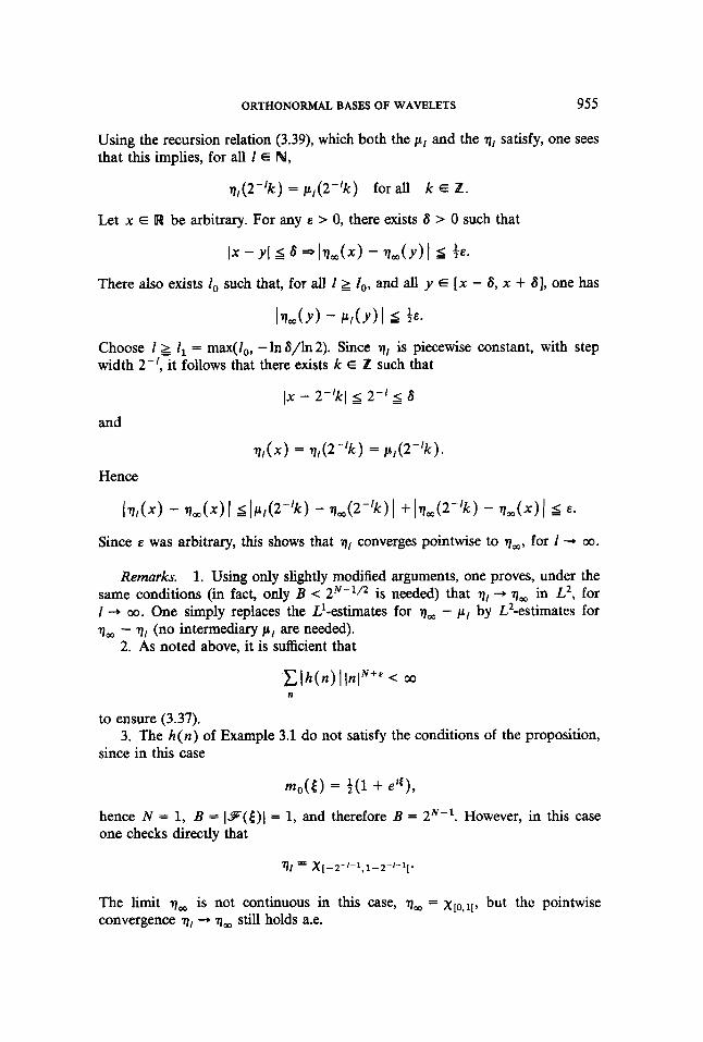
Using the recursion relation (3.39, which both the pI and the qr satisfy, one sees that this implies, for all I E N,
q,(2-'k) = pI(2-'k) for all k E H .
Let x E W be arbitrary. For any E > 0, there exists 6 > 0 such that
IX - YI I 6 + lqm(x> - t m ( Y ) I s tea
There also exists I , such that, for all I1 I, , and all y E [ x - 6, x + 61, one has
Jqm(y) - P / ( Y ) I I t ~ * Choose I >= I , = max(l,, -1nS/ln2). Since q, is piecewise constant, with step width 2-', it follows that there exists k E Z such that
and
Hence
I X - 2-'k( 5 2-' 6
q r ( x ) = ql(2- 'k) = pI (2 - 'k ) .
Remarks. 1. Using only slightly modified arguments, one proves, under the same conditions (in fact, only B < 2N-1/2 is needed) that qr + qm in L2, for I -+ co. One simply replaces the L'-estimates for q, - p l by L2-estimates for qm - q1 (no intermediary p r are needed).
2. As noted above, it is sufficient that
Clh(n)lInlN+" < co n
to ensure (3.37).
since in this case 3. The h ( n ) of Example 3.1 do not satisfy the conditions of the proposition,
rn,(() = $(I + d t ) ,
hence N = 1, B = 19(()1 = 1, and therefore B = Z N - ' . However, in this case one checks directly that
The limit q, is not continuous in this case, qm = x [ , , ~ [ , but the pointwise convergence q, -+ q, still holds a.e.
956 I. DAUBECHIES
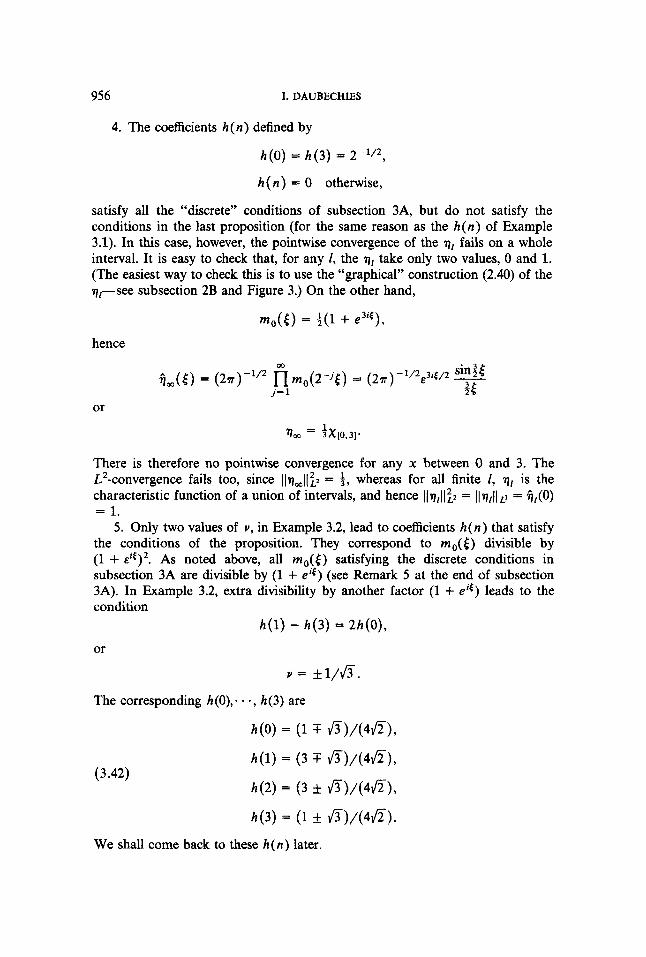
4. The coefficients h ( n ) defined by
h(0) = h(3) = 2-1’2,
h( n) = 0 otherwise,
satisfy all the “discrete” conditions of subsection 3A, but do not satisfy the conditions in the last proposition (for the same reason as the h ( n ) of Example 3.1). In this case, however, the pointwise convergence of the q, fails on a whole interval. It is easy to check that, for any I, the qr take only two values, 0 and 1. (The easiest way to check this is to use the “graphical” construction (2.40) of the q,-see subsection 2B and Figure 3.) On the other hand,
mo([) = +(I + e 3 9 ,
hence
or
There is therefore no pointwise convergence for any x between 0 and 3. The L2-convergence fails too, since llq,l1’,2 = $, whereas for all finite I, qr is the characteristic function of a union of intervals, and hence Ilqrll$ = llq,llL1 = ij,(O) = 1.
5. Only two values of Y, in Example 3.2, lead to coefficients h ( n ) that satisfy the conditions of the proposition. They correspond to mo([) divisible by (1 + do2. As noted above, all mo([) satisfying the discrete conditions in subsection 3A are divisible by (1 + eiE) (see Remark 5 at the end of subsection 3A). In Example 3.2, extra divisibility by another factor (1 + eJE) leads to the condition
h(1) - h ( 3 ) = 2h(0),
Y = fl/&
h(0) = (1 r 6 ) / ( 4 4 3 ) ,
or
The corresponding h(O), . , h(3) are
(3.42)
We shall come back to these h ( n ) later.
ORTHONORMAL BASES OF WAVELETS 957
With Proposition 3.3 we have completed our program of writing a set of explicit conditions on the h ( n ) , g ( n ) , without reference to a multiresolution analysis background, which make Mallat’s algorithm work, and which moreover lead to filters with sufficient “regularity”.
In the case where the h ( n ) , g ( n ) are calculated starting from a multiresolu- tion analysis (see subsection 2C), one has
h ( n ) = (+ lo , +on>,
or
i.e.,
+ ( t x ) = 2ll2 C h ( n ) + ( x - n). n
This is equivalent to
It follows that
(3.43)
or, since &O) = ( 2 ~ ) - ~ / ’ / dx + ( x ) = (27r)-’/’ (see (2.18)),
(3 -44) 44.) = r)&)*
As pointed out in subsection 2B, the r), = T ~ x [ - ~ / ~ , ~ / ~ [ can also be computed via a different recursion, ( 2 4 , which we shall call the “graphical” recursion, and which lies at the basis of the graphical construction technique illustrated by Figure 3. It follows from (3.44) that, in the case where the h ( n ) are derived from a multiresolution analysis framework, the graphical construction by iteration (see Figure 3, where the h ( n ) now play the role of the w ( n ) ) is therefore nothing but a reconstruction of the function +; in the limit for 1 -+ 00, finer and finer detail is achieved for increasing 1.
3.C. Equivalence between the discrete conditions and multiresolution analy- sis. So far we have formulated conditions, directly on the h ( n ) , which ensure that S. Mallat’s algorithm works (with these coefficients), and has regularity (in the sense given to it at the end of subsection 2B, or in subsection 3B). We have seen for every condition how the coefficients h ( n ) computed from a multiresolu- tion analysis fit into the picture. The main result of this subsection is that these multiresolution-based examples are the on& ones. It turns out that any sequence
958 I. DAUBECHIES
of h ( n ) satisfying the conditions in subsections 3A and 3B corresponds to a multiresolution analysis. The function 7" defined by (3.26) is then exactly the function + from the multiresolution structure.
To prove this equivalence, we start from a sequence h ( n ) satisfying (3.18), (3.19) and (3.27). We also assume that the function rno(<) = 2-'I2Cnh(n)ein6 satisfies all the conditions in Proposition 3.3. We then define, as in (3.17),
(3.45) g ( n ) = ( - l ) " h ( - n + I) ,
and, as in (3.44),
or
m
(3.46) 4(<) = (2")-112 n r n o ( 2 - j t ) . j = 1
From the proof of Proposition 3.3 we know that + is a bounded, uniformly continuous function; since 4 E L' n L", one also has + E L2. We define, in accordance with (2.16),
(3.47)
Since Cnlg(n)l = C,lh(n)l < 00, it follows that
All the estimates of subsection 3B on 7, carry over, therefore, to +, and one finds that J, is a bounded, uniformly continuous L*-function. As before, we define +jk(X) = 2-JI2 +(2-jx - k ) , and +jk(X) = 2-J12 +(2-jx - k ) . The defi- nitions (3.46) and (3.47) immediately imply
(3.48)
(3.49)
We shall prove that the +jk constitute an orthonormal basis of L2(W). In a first step we prove some orthogonality relations.
LEMMA 3.4. Let h(n) satisfy (3.18), (3.19), (3.28) and the conditions in Proposition 3.3. Let g ( n ) , +, + be dejined by (3.459, (3.46), (3.47), respectively.
ORTHONORMAL BASES OF WAVELETS 959
Then $, # E L 2 ( W ) , and, for all j, k , k' E h,
(3.50) ( # j k , # j k ' ) = ' k k ' ,
(3.51) ( # j k , $jk') = O,
(3.52) ($ jk? $jk') = ' kk"
Remark. Note that (3 .50)-(3.52) are restricted to one j-level at a time. The orthogonality between j-levels will follow from Lemma 3.5.
Proof: 1. Let f r be defined as in Proposition 3.3,
For reasons which will become obvious, we add an index 0 to f r ,
f r .0 = 771.
For arbitrary k E Z, we define
f/, k = ( T k ) ' X [ - 1/2+ k , 1 /2+ k [
with ( T k f ) ( x ) = @ Z n h ( n ) f ( 2 x - n - k). Due to the translations over k , built into qo, k as well as into Tk, qr, k is just a translated version of This can easily be checked by induction,
f O , k ( x ) = x [ - 1 / 2 + k , l / 2 + k [ ( x ) = f O , O ( x - k ,
and
f l , k ( x ) aCh(n)f/-1,k(2x - - k , n
Since (see Remark 1 following Proposition 3 . 3 ) I I f r , o - $llLz -+ 0 for I .+ 00, it
2. Since i j , , o ( E ) = [ n j _ , m 0 ( 2 - j ~ ) ] ~ 0 , 0 ( 2 - r E ) , and since I rno(E) I s 1 and folh's that Ilf,, k - $OkllL2 0 for 1 b o a
E L ~ , it follows that all the f r , k are in L2.
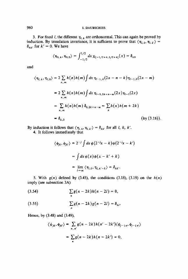
960 1. DAUBECHIES
3. For induction. ' k k ? for k'
fixed I, the different qr, are orthonormal. This can again be proved by By translation invariance, it is sufficient to prove that (v/, k , vr, k ' ) = = 0. We have
and
By induction it follows that ( q / , k , r)/, k ' ) = ' k k ! for all I , k , k'. 4. It follows immediately that
( + j k , +jk,) = 2-'/&+(2-'x - k)+(2-'x - k')
= / ~ x + ( x ) + ( x - k' + k )
5 . With g ( n ) defined by (3.49, the conditions (3.18), (3.19) on the h ( n ) imply (see subsection 3A)
(3.54)
(3.55)
C g ( n - 2 k ) h ( n - 21) = 0, n
Hence, by (3.48) and (3.49),
= C g ( n - 2 k ) h ( n - 2k') = 0 , n
ORTHONORMAL BASES OF WAVELETS 961
and
The “discrete orthogonality condition” (3.18) plays a crucial role in this proof. In the terminology of subsection 3A, (3.18) is equivalent to HH* = 1, where H* is the bounded I2-operator (see subsection 3A)
This implies that H*, as an operator from l 2 to 12, preserves orthogonality of sequences. The operator TH defined by (3.24) was in fact constructed to exactly reproduce, when acting on xi-1,2,1,2[ and its iterates, the action of H* on the sequence e ( e n = an0) and its iterates (see subsection 2B). This implies that repeated application of TH preserves the orthogonality of the qlo,k. This is what makes the above proof work.
In the following lemma we prove that the +,k constitute a tight frame (see Section 1, or (3.57) below). Again, the crucial ingredient will be one of the discrete identities which follow from the conditions on h( n ) , g( n) . From subsec- tion 3A we know that, with g ( n ) as defined by (3.49, and with h ( n ) satisfying all the conditions above,
(this can also be derived directly from (3.18) and (3.45)). It follows that (use (3.48), (3.49))
This, of course, already points towards multiresolution analysis (see subsection 2A).
LEMMA 3.5. Let h ( n ) , g (n ) , +, + be as in Lemma 3.4. Then, for all f E L2(W),
(3.57)
962 I. DAUBECHIES
Proof: 1. Take any f E CF, Then, since + E L', Xnl(+jn, f ) I 2 converges, for a n y j E Z. Moreover, by (3.56),
where we have used (3.18), (3.54) and (3.55). 2. By iteration, one has, for all N E N,
N c c 1 ( + j k , f) 1 2 - (3.58) c 1 ( G - N n , f) 1' = c 1 ( + N k , f) 1' + n k j = - N k
In this expression we shall let N tend to GO. 3. We first concentrate on C k l ( + N k , f > 1 2 . Let us suppose, for the sake of
definiteness, that suppf c [ - 2 " o , 2"0]. Take N 2 no + 1, so that the translation steps in the + N k ( x ) = (pN0(x - 2 N k ) are larger than Isuppfl. On the other hand, for any E > 0 there exists k, E N such that
Then
s 2 - N ( 2 k , + l)lr+lr: Ilfll: + E l l f l l l .
By choosing E and N appropriately, this can be made arbitrarily small. Hence
(3.59) C I ( + N k 3 f > 1 2 '*
k
ORTHONORMAL BASES OF WAVELETS 963
4. We now concentrate on & l ( + - N k , f ) I 2 . By means of the Poisson formula this can be rewritten as
Here
An easy estimation then leads to
This tends to zero for N + 00.
5. We now examine the first term in (3.60). One has
since lrno(3)1 5 1 for all 3 E R. But
- - < ClSI",
where we have used (3.19) and (eiu - 11 5 CeIale (we assume 0 < E 5 1). Hence,
m
- i (0 ) 1 6 (2a)-'l2C c (2-jtle I - C'gy. j - 1
964 I. DAUBECHIES
Consequently, using i(0) = (2~)-"', we find
2 n j dE ( 6 ( m ) I'lf(t) I'
This converges to l l f l l ' as N + 00. Hence
(3.61) c I ( + - N k , f) l2 llf11'. k
6. Putting together (3.58), (3.60) and (3.61) shows that, for all f E CT(R),
(3.62) C I ( + j k , f) I' = I I ~ I I ~ L ~ . j , k
Since CT(R) is dense in L2(R), (3.62) extends to all f E L2(R).
Since 11+11 = 1 (this is a special case of (3.50), with j = k = k' = 0), (3.57) implies that the + jk constitute an orthonormal basis. This completes the proof of the main theorem of this section.
THEOREM 3.6. Let h ( n ) be a sequence such that
(i) Cnlh(n)l lnl' < 00 for some E > 0, (ii) Cnh(n - 2k)h(n - 21) = Sk,,
(iii) C h ( n ) = 2ll2. Suppose also that mo( t ) = 2 - '/'Cn h (n) e in€ can be written as
ORTHONORMAL BASES OF WAVELETS 965
Then the + j ’ j k ( ~ ) = 2-JI2+(2-Jx - k ) define a multiresolution analysis (in the sense of subsection 2A); the qjk are the associated orthonormal wavelet basis.
Remarks, 1. As we already said in the introduction, this theorem is also proved in [19], under slightly different conditions. The growth restrictions (3.37) and (3.38) on the h ( n ) are replaced, in [19], by the condition that
this condition implies that the +jk, with Cp defined as above, define a multiresolu- tion analysis. The function + may, however, still be very irregular; the coefficients h ( n ) used in Figure 4, e.g., satisfy the positivity condition of [19], but are clearly not associated with a regular +. In the present paper, we emphasized regularity of the discrete filters; once regularity is ensured by means of conditions (3.36)-(3.38), equivalence with regular multiresolution analysis follows. Consequently, the techniques of our proofs and the proofs in [19] are quite different. The basic intuition for the present proof was mainly graphical. As explained above, the orthogonality of the +oOk follows naturally, given our “graphical” construction, from the discrete conditions. Similarly, (3.60) can be understood graphically.
2. At the end of subsection 3B (Remark 3) we mentioned the link between the present construction and the “conjugated quadrature filters” of Smith and Barnwell [24]. Any of their conjugated quadrature filters will satisfy all the conditions in subsection 3A. Provided they also satisfy the regularity condition in subsection 3B, they can be used to construct orthonormal wavelet bases. Since the goals of [24] are completely different however, most of the examples in [24] do not satisfy our regularity condition.
infl&l*,/21m,(Ol > 0. Together with lmo(t>I2 + Imo(l + n)I2 = 1, m,(O) = 1,
4. Orthononnal Bases of Wavelets with Compact Support
In subsection 2A we reviewed how orthonormal bases of wavelets can be constructed, starting from a multiresolution analysis framework. The basic in- gredient there was a function + such that (2.15) held, for some c,, without even requiring the to be orthogonal. Theorem 3.6 gives another recipe for con- structing an orthonormal basis of wavelets (and the associated multiresolution analysis), this time from a sequence ( h ( n ) ) , EZ.
If this sequence has finite length, h(n) = 0 for n < N - , or n > N , , then the corresponding basic wavelet has compact support. This can be checked very easily from the graphical construction of + (see Figures 2,4), or from the recursive definition of the q,,
(4.3) v o = X[-1/2,1/2[.
966 I. DAUBECHIES
The recursive definition of the qr implies that all the qr have compact support, SUPP v/ c [Nl, -, Nl, +I , with Nl, -= t (Ni -1 , -+ N-1, and NI, += t (Nr-1 , ++ N+h while No, -= - 5, No, += $. Hence H/, - + N - , Nr, + + N + for 1 + 00, which implies that (p has compact support c [ N - , N+]. Since only finitely many g ( n ) are non-zero ( g ( n ) = 0 for n < - N + + 1 or n > - N - + l), J, also has compact support,
supp J, c [+(l - N + - N - ) , t (1 + N + - N - ) ] .
In order to construct orthonormal bases of compactly supported wavelets, it suffices, therefore, to construct finite-length sequences h (n) satisfying all the conditions of Theorem 3.6. An example of such a finite-length sequence is Example 3.2, with v = f 1 / f i (see Remark 5 following Proposition 3.3). In this case one finds (see (3.42)) N - = 0, N + = 3, and
(4.4)
Since
the example (3.42) satisfies all the required conditions. The h ( n ) given by (3.42) correspond, therefore, to an orthonormal basis of continuous wavelets. The basic wavelet has support width equal to N+- N - = 3. Figure 5 shows the graphs of (p, J, and their Fourier transforms, for this example. There are several striking features in Figure 5. First of all, it is obvious that even though and J, are continuous, they are not very regular. There exist other constructions of com- pactly supported wavelet bases, in which c) and + have more regularity, at the cost of larger numbers of non-zero coefficients h ( n ) , which results in larger support widths for +, (p. For the family of examples we shall examine below, the support width of J,, c) increases linearly with their regularity. Another striking feature of Figure 5 is the lack of any symmetry or antisymmetry axis for J,, (p. This is quite unlike the Meyer wavelets (see [4]) or the Battle-LemariC wavelets (see [16]). In all these (non-compactly supported) examples, (p is an even function, and J, is symmetric around x = f. We shall see below that, except for the Haar basis (see (1.9) or Example 3.1), there exist no compactly supported wavelet bases in which c) is either symmetric or antisymmetric around any axis.
The plots of J, and c) in Figure 5 (and later figures, for other examples) are made by direct implementation of the “graphical recursion algorithm” equivalent with (4.1)-(4.3) (see subsection 2B). This is much more efficient than Fourier transform of the infinite product (3.46) (see [26]). To plot Figure 5 , only 8 iterations of type (2.40) were needed (i.e., qs is plotted rather than (p; the
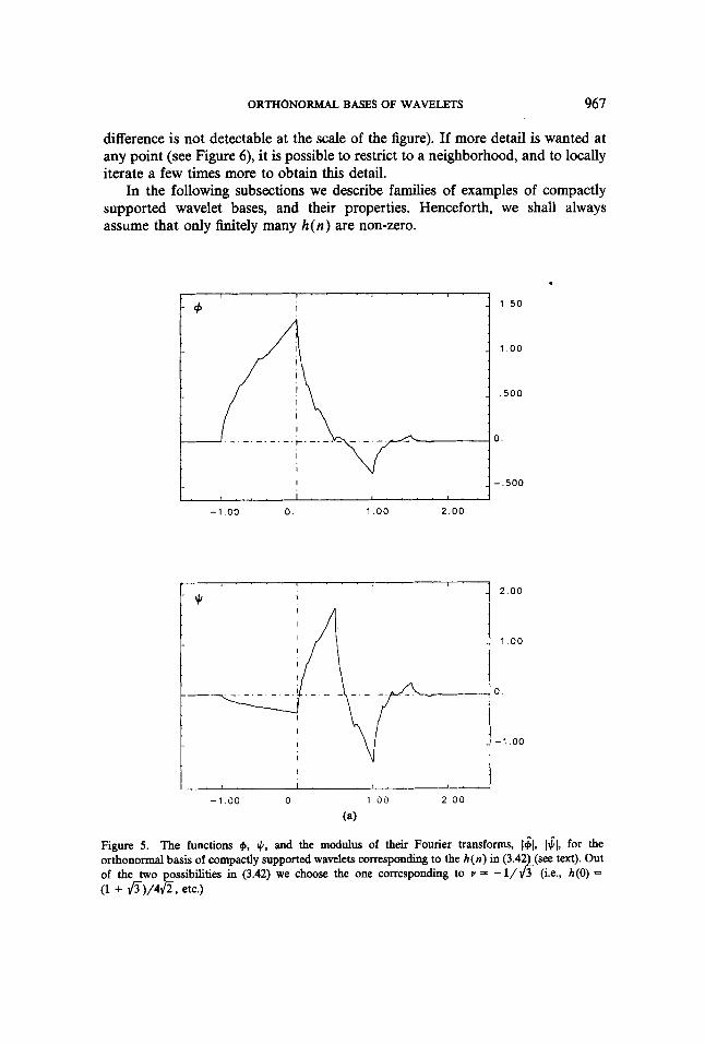
ORTHONORMAL BASES OF WAVELETS 967
I
: 9 I
I
I 4 . . :
difference is not detectable at the scale of the figure). If more detail is wanted at any point (see Figure 6), it is possible to restrict to a neighborhood, and to locally iterate a few times more to obtain this detail.
In the following subsections we describe families of examples of compactly supported wavelet bases, and their properties. Henceforth, we shall always assume that only finitely many h ( n ) are non-zero.
2.00
1 .oo
0.
-1.00
1 . s o
1 . oo
,500
0.
-.so0
(a)
Figure 5. The functions 4, I), and the modulus of their Fourier transforms, $1, Ijl, for the orthonormal basis of compactly supported wavelets corresponding to the h ( n ) in (3.42) (see text). Out of the two ossibilities in (3.42) we choose the one corresponding to Y = -1/6 (i.e., h(0) =
(1 + fi)/4&, etc.)
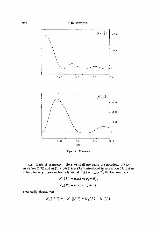
968 I. DAUBECHIES
,750
,500
, 2 5 0
0.
1 1
0 5 0 0 10 0 15 .0 20 0
(b)
Figure 5. Continued
4.A. Lack of symmetry. Here we shall use again the notations a(n); - -, d ( n ) (see (3.7)) and a([); - -, a(() (see (3.9)) introduced in subsection 3A. Let us define, for any trigonometric polynomial P(() = Cnp,,ernt, the two numbers
N + ( P ) = max{n; P,, f O},
N - ( P ) = min{n; p,, z O}. One easily checks that
N+(IPI2) = - N - ( I P I Z ) = N + ( P ) - N - ( P ) .
ORTHONORMAL BASES OF WAVELETS 969
Since Ia(E)12 + IP(E)12 = 1 (see (3.14)), and a # 0, /3 # 0 (see (3.15)), this implies
(4.5) N + ( 4 - N - b ) = N+(B) - N A B ) .
N+(mo) = m=(2N+(4,2N+(B) + 11,
N - ( m o ) = min(2N-(cu), 2N-(P) + 1).
On the other hand, the definition (3.7) of the a(n), b(n) , gives
Together with (4.5) this leads to
N + ( m o ) - N-(mo)
= max(2l\r+(a) - 2 ~ - ( / 3 ) - 1 , 2 ~ + ( / 3 ) - 2 ~ - ( a ) + 1). (4.6)
In any case, N + ( m , ) - N - ( m , ) is an odd number. If the function + were symmetric around zero, $ J ( x ) = $J( - x ) , then h ( n ) =
h ( - n ) would follow. This would however imply N + ( m o ) = - -N-(m0) , i.e., N+(mo) - N - ( m o ) = 2N+(mo) would be even. Since this is in contradiction with (4.6), it follows that the function 9, associated with an orthonormal basis of wavelets with compact support, can never be an even function.
What about symmetry with respect to another point A # O? Suppose
$0 + 4 = $J(A - 4, where we can, without loss of generality, shift X to the interval ]0,1[. Then it follows that
4(1) = e2i’4$( -t).
Because of the definition of 4 as the infinite product (3.46), this implies
mO(E) = ezr ’h0( - E ) .
Since both m o ( [ ) and mo(-[) are trigonometric polynomials, this leaves only one possible value for A, namely A = f?-. Let us, therefore, assume that $J is symmetric with respect to f,
Then
+ ( x + 1) = $J( - x ) .
h(2n + 1) = h( - 2 4 ,
or
b ( n ) = u ( - n ) .
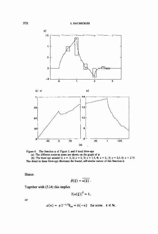
970 I. DAUBECHIES
a) 1.5
I .
.5
0
-.5
Figure 6. The function $I of Figure 5, and 6 local blow-ups (a) The different zoom-in zones are shown on the graph of + (b) The blow-ups around 1) x = .5, 2) x = 1, 3) x = 1.5, 4) x = 2., 5 ) x = 2.5, 6) x + 2.75.
The detail in these blow-ups illustrates the fractal, self-similar nature of this function +.
Hence - P ( 0 = 4 6 ) *
Together with (3.14) this implies
2 l G ) I’ = 1, or
a(.) = f2-1/2S,, = b ( - n ) for some k E N.
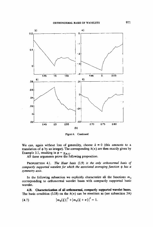
ORTHONORMAL BASES OF WAVELETS 971
1.45 1.5 1.55
I I ,021 I
2.45 2.5 2.55
(b)
Figure 6. Continued
We can, again without loss of generality, choose k = 0 (this amounts to a translation of @ by an integer). The corresponding h(n) are then exactly given by Example 3.1, resulting in Q = x ~ , , ~ ] .
All these arguments prove the following proposition.
PROPOSITION 4.1. The Haar basis (1.9) is the only orthonormal basis of compactly supported wavelets for which the associated averaging function Cp has a symmetry axis.
In the following subsection we explicitly characterize all the functions rn, corresponding to orthonormal wavelet bases with compactly supported basic wavelet.
4.B. Characterization of all orthonormal, compactly supported wavelet bases. The basic condition (3.18) on the h(n) can be rewritten as (see subsection 3A)
(4.7) Im,(€) IZ + Im,(€ + 4 l2 = 1.
972 I. DAUBECHIES
On the other hand, we have imposed, in Proposition 3.3, the following structure on m,:
(4.8) m O ( t ) = [$(l + e")] "Q(e"),
where Q is a polynomial, since only finitely many h ( n ) are non zero. Moreover, since all the h(n) are real, all the coefficients in Q are real as well. From (4.8) we have
lmo(E) l2 = [c0s2$t] NIQ(e'E) 12. Since Q(e '€ )= Q(e-"), the polynomial lQ(eiE)I2 can be rewritten as a poly- nomial in cost, or, equivalently, as a polynomial in sin2+[. Introducing the shorthand y = cos2$[, (4.7) becomes
(4.9) yNP(1 - y ) + (1 - y)"P(y) = 1.
Any m , of type (4.8) which solves (4.7) corresponds therefore to a polynomial P solving (4.9) and satisfying
(4.10) P ( y ) 2 0 for y E [0,1].
Conversely, every polynomial P satisfying both (4.9) and (4.10) leads to solutions of (4.7), with real coefficients h(n).This is due to the following lemma of Riesz [27].
LEMMA 4.2. Let A be a positive trigonometric polynomial containing only cosines, A ( ( ) = Er-,a,,cosn( (with a , E R). Then there exists a trigonometric polynomial B, of order N , B ( [ ) = Cr=,b,,eint, with real Coefficients b,,, such that
The proof of this lemma (see [27]) is simple and elegant. It constructs B explicitly; this construction is now widely used by engineers when designing filters. We include the proof here, because we shall come back to the construction later.
Proof: To
l N A ( ( ) = a, + c an(einC + e-i"E)
n-1
ORTHONORMAL BASES OF WAVELETS 973
we associate the polynomial
l N 1 N-1 pA(z ) = 2 QN-nZ" + aOzN + 2 anZN+,.
n-0 n - 1
This polynomial has 2N zeros (counting multiplicity). Since PA(eic) = eiNcA([), it follows that the two polynomials PA(z) and z"P,(z-') agree on the unit circle, and therefore on the whole complex plane. They have therefore the same zeros. This means that if zo is a zero of P&), PA(zo) = 0, then so is z;'. On the other hand, since the a, are real, PA( z ) = PA(?). This implies that if zo is a zero of PA(z), then so is its complex conjugate Zo. The zeros of P,(z) therefore come in quadruplets, to, Zo, z;' and Z i l , or (if zo = r, is real) in duplets, ro, r;l E R. Let z j , Zj, z,:', 2,:' be the quadruplets of complex zeros of PA(z), and rk, r;' the real duplets,
)I J n ( z - Z i ) ( Z - .,)(z - z;')(z - q1 [ j - 1
where
K J
k-1 j - 1
2
is clearly a trigonometric polynomial of order N with only real coefficients.
974 I. DAUBECHIES
Remarks. 1. Note that B is generally not unique. Out of any quadruplet of zeros zo, Zo, zil, 2,’ one can choose the pair of zeros to retain, for the construction of B, in four different ways. For every duplet of real zeros of PA two choices are possible. This results in 2N different possibilities for B.
2. All these different possibilities, corresponding to different choices of the zeros of PA to retain for B , constitute, however, the only solutions to (4.11). One can show (see [27]) that, up to an arbitrary phase factor f e i K 6 , K E E , all the polynomials B satisfying (4.11) are necessarily of the form (4.12).
If P is a polynomial satisfying (4.9) and (4.10), then Lemma 4.2 tells us that there exists a trigonometric polynomial of the same order such that
It follows that mo(.$) = [$(l + ei6>lNQ(ei6) satisfies (4.7). If, moreover,
then all the conditions of Theorem 3.6 are satisfied, and there exists an associated orthonormal wavelet basis.
To construct compactly supported orthonormal wavelet bases, with m, of type (4.8), it is therefore necessary and sufficient to find polynomials P solving (4.9) and (4.10), which are moreover strictly bounded above by 22(N-1).
The following two combinatorial lemmas allow one to “guess” a particular solution of (4.9).
LEMMA 4.3.
Proof: Define s,,, k = z:-.( n rj). Then
( n + j + l ) - (k + n + 2)! ( n + J ) ! ‘,+I, k+l - ( k + l ) ! (n + l)! + zo ( n + l ) ! j !
( n + J ) ! = ( ;: t 2, + + c ( n + l ) ! (J - l ) !
5’1
k + n + 2 ) - ( k + ’ ; + l ) ] ) + sn, k + [ %+l, k+l - ( k + l
ORTHONORMAL BASES OF WAVELETS 975
Hence
LEMMA 4.4.
n + j
J'O
Proof: Define A,,, = ( j ) . Then, by Lemma 4.3, cikm0 A,,, = A,+1, k.
Define
n + j S J y ) = i ( ) [ Y J ( l - y ) " + l +y"+'(l -y)'].
j - 0
Clearly, So(a) = (1 - a ) + a = 1.
We shall prove that & ( a ) = Sn-l(u), which proves the lemma. By repeatedly inserting factors [(l - a ) + a ] = 1, we find
n - 1 S,-,(a) = c An-l , j[(l - a ) " d + a"(1 - u)j ]
j - 0
n-1 = c A,,, j[(l - a)ntlaj + a*+' (1 - a) j ]
j - 0
+2A",,_,[(l - a)"+'a" + U " + ' ( l - a)"]
= s,,(a) (since2An,"-, = A,, , , , ) .
976 I. DAUBECHIES
It follows that the polynomial of order N - 1,
(4.13)
solves (4.9). Since all the coefficients in this polynomial are positive, (4.10) is clearly also satisfied.
The two explicit examples of compactly supported wavelet bases we have seen so far, i.e., Example 3.1 and (3.42), correspond exactly to a polynomial of type (4.13), with N = 1, 2, respectively. For Example 3.1 one has r n o ( ( ) = f ( 1 + eit) , i.e., N = 1 , and Q(e'[) = 1, hence P ( y ) = 1 = Pl(y) . For the second example (3.42), we find (see (4.4)) r n o ( [ ) = [ f ( l + eit)l21[(1 T 6 ) e i t ] , corresponding to N = 2 and lQ(eit)12 = 2 - cos [ = 1 + 2sin2$(; hence P ( y ) = 1 + 2y = P 2 ( y ) .
In fact, for given N , PN is the only polynomial of order less than N which solves (4.9). Even more is true: for any polynomial P solving (4.9), the first N terms (orders 0 up till N - 1) are exactly given by PN. This is because (4.9) completely determines the first N coefficients po, - - -, p N P 1 in P ( y ) = Zf=opny". Since the first term in (4.9) is already of order N , only the second term plays a role in the cancellations for y", k = 0, - . -, N - 1. This leads to
Po = 1 ,
k = l , . , . , N - 1,
from which the P k , k = 1,- - ., N - 1, can be determined recursively. Since P,,, solves (4.9), it follows from (4.13) that
Consequently, any polynomial P solving (4.9) is of the form
(4.15) P ( Y ) = P,,,(Y) + Y W Y ) .
Substitution of (4.15) into (4.9) leads to the following equation for the poly- nomial R :
Y N ( l - y ) N R ( l - Y > + ( 1 - Y ) N Y N K Y ) = 0, or
R ( l - JJ) + R ( y ) = 0.
The polynomial R is therefore antisymmetric with respect to y = i, or
R ( Y ) = fie - - Y L
where I? is an odd polynomial.
ORTHONORMAL BASES OF WAVELETS 977
To summarize, we have the following explicit characterization of all solutions m , of (4.7), corresponding to only finitely many non-zero h(n) .
PROPOSITION 4.5. Any trigonometric polynomial solution m , of (4.7) is of the form
(4.16)
where N E N, N 2 1, and where Q is a polynomial such that
m , ( [ ) = [f(1 + e 'P) ]NQ(e 'E) ,
(4.17) ( Q ( e i P ) l2 = kl( -: + k)sin2k+( + [sinZN+[] R ( f c o s [ ) , k - 0
where R is an oddpolynomial.
Remarks. 1. Since the proof of Lemma 4.2 shows explicitly how to construct all possible polynomials Q once lQ(eiP)I2 is known, t h i s proposition is indeed an explicit characterization of all the solutions m , of (4.7).
2. In constructing m,, there are therefore 3 steps at which choices can be made,
(i) choosing N E N \ {0}, (ii) choosing an odd polynomial R (with some restrictions), (iii) choosing pairs of zeros out of each quadruplet of complex zeros, and one
zero out of each duplet of real zeros, of PN(z) + z N R ( z - +) (see the proof of Lemma 4.2).
The odd polynomial R cannot be chosen completely freely. One needs, of course, the fact that
(4.18) ~ , ( y ) + y N ~ ( $ - y ) 2 0 for 0 s y 6 I .
Moreover, condition (v) in Theorem 3.6 requires that
(4.19) SUP [ M Y ) + Y N R ( f - y ) ] < 22"-1)* 04Y61
3. For N = 1, (4.16), (4.17) and (4.18) reduce to
(4.20)
with
m o ( ( ) = f(l + e iE)Q(e i t )
(4.21) ( e (e iPI2= 1 + sin2$[R(fcos(),
where R is an odd polynomial such that
978 I. DAUBECHIES
These conditions can already be found in the construction of conjugate quadra- ture mirror filters in [24]. The condition (4.19) is impossible to satisfy, however, because Pl(0) = 1.
4. Using a different method, Y. Meyer constructs in [28] another polynomial solving (4.7). The solutions to (4.7) proposed in [28] are
(2N - l ) ! (4.22) Imo(E) I 2 = 1 - 2N-1 fsinZN-’xdx.
[ ( N - l)!] 2
This is clearly an even trigonometric polynomial of order 2 N - 1. It turns out to be divisible by (i(1 + cos ())N = ( c o s ~ $ $ ) ~ . Therefore, by Proposition 4.5, (4.22) is exactly equal to
(cos’tt) N ~ N (sinzit).
4.C. A family of examples with arbitrarily high regularity. In the remainder of this section, we shall concern ourselves with a special family of functions mot and the corresponding wavelet bases. We follow the prescriptions of Remark 2 after Proposition 4.5. For every N E N, N 2 1, we choose Q of minimal order, i.e., R = 0, lQ(eit)12 = PN(sinz+E). This choice satisfies both the conditions (4.18) and (4.19). From (4.13) the positivity of P N ( y ) for 0 4 y 4 1 is immediate. Since PN is strictly increasing for y 2 0, it follows that
where we have used Lemma 4.3 in the second equality. This fixes lQ1’. In the construction (via Lemma 4.2) of Q from lQI2, we systematically retain all the zeros inside the unit circle (this corresponds to a “minimal phase” choice in filter design). For N E N, N > 1 fixed, this determines Q unambiguously, up to a phase factor eiKt , K E H. For the sake of definiteness we fix this phase factor so that Q contains only positive frequencies, starting from zero, i.e.,
(4.24) Q N ( e i t ) = qN(n)e int with 40 # 0.
These choices uniquely determine Q N . We shall denote the corresponding m, by
N - 1
n - 0
N m O , N-1
, m O ( t > = [+(I + e i t ) l N c qN(n)e in6 n - 0
2N-1 = 2-lI2 C hN(n)e’nl .
n - 0
ORTHONORMAL BASES OF WAVELETS 979
Table 1 lists the coefficients h,(n) for the cases N = 2,3; - ., 10. For the lowest values of N, QN(E) can be determined analytically. One has, e.g.,
Q 2 ( E ) = $[(I + 0) + (1 - 0 ) e i c ] (see (4.4))
and
~ ~ ( 6 ) = +[(I + m + JGiEiT) + 2(1- m > e i c
+ (1 + - & F $ i T ) e 2 ' ~ ] .
For larger values of N, the coefficients in Table 1 were computed numerically. Since the NmO satisfy all the conditions of Theorem 3.6, there exists an
associated orthonormal basis of continuous wavelets with compact support for every NmO. Let us denote the corresponding I+, + functions by N+, N+. Since h,(n) = 0 for n < 0 and n > 2N - 1, it follows (see the discussion at the start of Section 4) that supp(,+) = [0 ,2N - 11. The support of N+,
2N- 1
( N + > ( X ) = c ( - 1 ) " U - n + 1)NI+(2X - 4, n - 0
is therefore given by [ - (N - l), N]. Note that an additional phase factor eiKe, K E Z, in (4.24) would amount to shifting the h,(n) by K , i.e., to shifting the function N~ by an integer, which does not aff'ect the multiresolution analysis construction. The wavelet N+ is unaff'ected by this shift.
From Theorem 3.6, we know that N+ and N+ are bounded, continuous functions. For large N , N+ and N+ are, in fact, much more regular. To see this, we shall need the following generalization of Lemma 3.2.
LEMMA 4.6. If mo(E) = [$(l + eit)lN 9((), where 9(() = Cnfneine satisfies
(4.25)
(4.26)
then
(4.27)
Proof Define
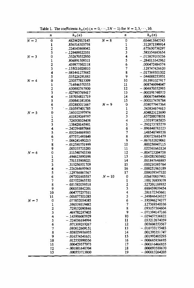
N = 4
N = 5
N - 6
Table 1. The coefficients h , (n) (n = 0,- * - , 2 N - 1) for N = 2,3, * . . , lo.
n h,(n) n h , (n) N - 2 0 .482962913145 N = 8 0 .054415842243
1 336516303738 1 .312871590914 2 .224143868042 2 .675630736297 3 - .129409522551 3 .585354683654
N - 3 0 .332670552950 4 - .015829105256 1 .806891509311 5 - .284015542962 2 .459877502118 6 .000472484574 3 - .135011020010 7 .128747426620 4 - .085441273882 8 - .017369301002 5 .03 5226291 882 9 - .044088253931 0 .230377813309 10 .013981027917 1 .714846570553 11 .008746094047 2 .630880767930 12 - .004870352993 3 - .027983769417 13 - .000391740373
5 .0308413 81 836 15 - .000117476784 4 - .187034811719 14 .000675449406
6 .032883011667 N = 9 0 ,038077947364 7 - .010597401785 1 .243834674613 0 .160102397974 2 .604823123690 1 .603829269797 3 .657288078051 2 .724308528438 4 .133197385825 3 S38428145901 5 - .293273783279 4 - .242294887066 6 - .096840783223 5 - .032244869585 7 ,1485407493 3 8 6 .077571493840 8 .030725681479
8 - .012580751999 10 .000250947115 9 .003335725285 11 .022361662124
7 - .006241490213 9 - .067632829061
0 .111540743350 12 - .004723204758 1 .494623890398 13 - .004281503682 2 .751133908021 14 .001847646883 3 .3 152503 5 1709 15 .O00230385764
5 - .129766867567 17 .oooO39347320 6 .097501605587 N = 1 0 0 .026670057901 7 ,027522865530 1 .1881768OOO78 8 - .031582039318 2 .527201188932 9 .000553842201 3 .688459039454
10 .004777257511 4 .281172343661
4 - .226264693965 16 - .O00251963189
11 - .001077301085 5 - .249846424327 N - 7 0 .077852054085 6 - .195946274377
1 .396539319482 7 .127369340336 2 .729132090846 8 .093057364604 3 .469782287405 9 - .071394147166 4 - .143906003929 10 - .029457536822 5 - .224036184994 11 ,033212674059 6 .071309219267 12 DO3606553567
8 - .038029936935 14 .001395351747 9 - .016574541631 15 .001992405295
7 .080612609151 13 - .010733175483
10 .012550998556 16 - .000685856695 11 .ooo429577973 17 - .000116466855
13 .O00353713800 19 - .ooOo13264203 12 - .001801640704 18 .ooOo93588670
ORTHONORMAL. BASES OF WAVELETS 981
Then
j - 1
Repeating the proof of Lemma leads to
3.2, with multiplication factor 2k instead of 2
This implies (4.27).
To interpolate between the standard spaces Ck of k times continuously differentiable functions, we shall use, for a 4 N, a > 0, the spaces defined by
(4.28) f € C" * I d " V( t ) 1(1 + Itl)"" < 00.
Note that, for a = k E N, the condition (4.28) implies f E Ck, but is not necessary.
We then have the following
PROPOSITION 4.7. There exists A > 0 such that, for all N E N, N 2 2,
(4.29) N + , N$ CAN*
Proof: We shall apply Lemma 4.6. Since QN(eiE) has only a finite number of terms, (4.25) is obviously satisfied. We compute
B, = suplQN(ei~)QN(ei6'z) I = sup IPN(sin2~E)PN(sin'at) I 1
= SUP ipN(4y(1 - Y ) ) p N ( Y ) I. 0s-Y 5 1
First, note that (see (4.28))
< 2XN-1). SUP M Y ) = M1) 06YS1
Secondly,
N - 1 5 c 2N+k-1yk 2N-1Nmax(l,(2y)N).
k-0
982 I. DAUBECHIES
[log N-N log(36/4)]/2 log 2 5 c ( 1 + IEl) This exponent is smaller than'-1 for N 2 16. For smaller values of N, one can use the explicit estimate
to prove that
I ( N + Y (0 1 4 c ( 1 + lwl-KN for some K > 0, for all N 5 16. Hence (4.29) holds for &, for some X > 0, and for all N 2 2. Since NI+b is always a finite linear combination of translated and dilated versions of the same holds for N + .
Remarks. 1. Since Isupp(,+)l = I~upp(~+)I = 2 N - 1, (4.29) shows that the regularity of &, N I + b increases linearly with their support width, as announced in the introduction. It turns out that linear increase of the support width with the regularity of +, I+b is the best one can do. More precisely, if a @-function + satisfies an equation of the type
N
+(.) = c cn+(2x - 4 n - 0
ORTHONORMAL BASES OF WAVELETS 983
(without necessarily being connected to multiresolution analysis), and if supp cp c [0, N], then k 5 N - 2. For a proof, see [30].
2. The estimate for A obtained in this proof is, of course, not very good; the argument is too simple. Asymptotically, for large N, one finds
with
log(%q + O ( 7 ) log N 2 .1887 + O ( 7 ) . log N p - 2log2
The same technique, with a little more work, leads to slightly better estimates if larger values of k are used. Using k = 4, e.g., leads to
P = > .1936 + O(N-’log N) .
Since the map y * 4y(l - y ) has a fixed point, at y = $, one finds
One can show that
PN( 2) - C3N.
Even for arbitrarily large k, the values of p obtained by this method are therefore limited by
p s 1 - - log 3 + O(N-’log N ) P .2075 + O(N-’log N) . 2 log 2
3. Using a more sophisticated method than the brutal estimates above, Y. Meyer [28] showed that, again asymptotically for large N,
with p = log(4/n)/log2 E .3485. His proof uses (4.22) rather than PN. 4. For small values of N, better estimates can be obtained for the regularity
of the &, N+ by yet a third method. This method is based on a generalization of a technique used by Riesz in the proof that “Riesz products” can lead to continuous, nowhere differentiable functions. I would like to thank Y. Meyer for introducing me to this technique, and for showing me how to use it to prove 2$J,2+ E C5-‘. The proof, and a generalization for N 2 3, are given in the Appendix. It works very well for small values of N, but does not, however, give good asymptotic results. For large N, it leads to logarithmic rather than linear increase of the regularity of the &, N+.
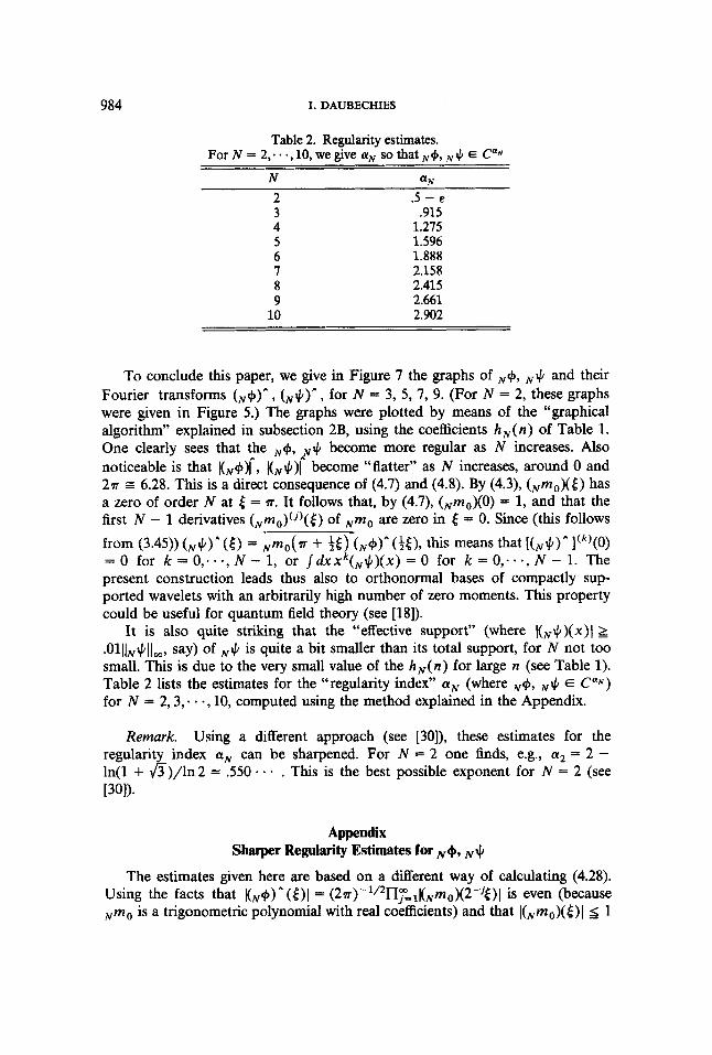
984 I. DAUBECHIES
Table 2. Regularity estimates. For N = 2,. . -, 10, we give aN so that ,,,+, N $ E CUM
N aN 2 .5 - &
3 4 5 6 7 8 9
10
.915 1.275 1.596 1.888 2.158 2.415 2.661 2.902
To conclude this paper, we give in Figure 7 the graphs of N+, N+ and their Fourier transforms for N = 3, 5, 7, 9. (For N = 2, these graphs were given in Figure 5.) The graphs were plotted by means of the “graphical algorithm” explained in subsection 2B, using the coefficients h , ( n ) of Table 1. One clearly sees that the &, N+ become more regular as N increases. Also noticeable is that I ( N + ) [ , I(,+)[ become “flatter” as N increases, around 0 and 27~ = 6.28. This is a direct consequence of (4.7) and (4.8). By (4.3), &m0)([) has a zero of order N at 6 = I T . It follows that, by (4.7), (Nmo)(0) = 1, and that the first N - 1 derivatives & m O ) ( j ) ( [ ) of N m o are zero in Z = 0. Since (this follows from (3.45)) ( N + ) A ( ( ) = Nmo(IT + $ 6 ) (N+)a($[), this means that [ (N+)A] (k ) (0 ) = 0 for k = O,..., N - 1, or / ~ x x ~ ( ~ + ) ( x ) = 0 for k = o,..., N - 1. The present construction leads thus also to orthonormal bases of compactly sup- ported wavelets with an arbitrarily high number of zero moments. This property could be useful for quantum field theory (see [MI).
It is also quite striking that the “effective support’’ (where I(N+)(x)l >= . O l ~ ~ N + ~ ~ m , say) of N+ is quite a bit smaller than its total support, for N not too small. This is due to the very small value of the h, (n ) for large n (see Table 1). Table 2 lists the estimates for the “regularity index” aN (where &, N+ E P N ) for N = 2,3; a , 10, computed using the method explained in the Appendix.
Remark. Using a different approach (see [30]), these estimates for the regularity index aN can be sharpened. For N = 2 one finds, e.g., a2 = 2 - ln(1 + fi)/ln 2 = 3 0 . - . This is the best possible exponent for N = 2 (see t301).
Appendix Sharper Regularity Estimates for N+, N+
The estimates given here are based on a different way of calculating (4.28). Using the facts that I(&)- ([)I = (27~)-’’~~~~~~(~m~)(2-’6)~ is even (because N m O is a trigonometric polynomial with real coefficients) and that I(Nmo)(Z)l 5 1
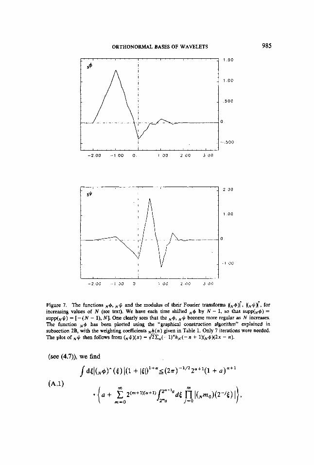
ORTHONORMAL BASES OF WAVELETS
' - 39 I
985
2 0 0
1 5 0
1 .oo
,500
0
-.500
-200 - 1 00 0 1 0 0 2 0 0 3 00
- 2 00 - 1 30 0 1 3 0 2 30 3 0 0
Figure 7. The functions ,+, ,+ and the modulus of their Fourier transforms I&@)[, I(,+)[, for increasing values of N (see text). We have each time shifted ,+ by N - 1, so that supp(,+) = supp(,+) = [ -(N - l), N]. One clearly sees that the &, ,# become more regular as N increases. The function N# has been plotted using the "graphical construction algorithm" explained in subsection 2B, with the weighting coefficients ,h (n ) given in Table 1. Only 7 iterations were needed. The plot of ,+ then follows from &#)(x) = &En(-l)"hN(-n + 1)(,$1)(2x - n) .
(see (4.7)), we find
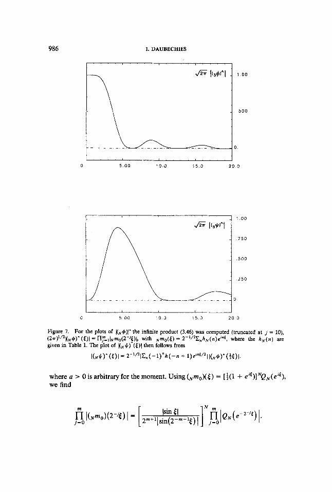
986 I. DAUBECHIES
9 5 90 10 0 1 5 i) 20 0
Figure 7. For the plots of b+)I ̂the infinite product (3.46) was computed (truncated at j = lo), (2a)'/21(~9)^ (€11 * n,"-lbm0(2-'9l, with NmO(€) = 2-1/2X,hN(n)e'"f, where the h , ( n ) are given in Table 1. The plot of LJI) ([)I then follows from
I (~+ ) - (€)I = 2-1/2~En (- 1)"h (- n + l)e'"f/21 I ( ~ + ) * (it) I.
where a > 0 is arbitrary for the moment. Using (Nrno)(E) = [ f ( l + ei6)]NQN(ei t ) , we find
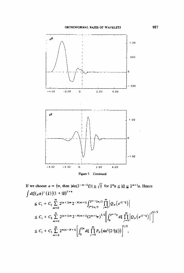
ORTHONORMAL. BASES OF WAVELETS
, . I
-
-
I
I . . . I . . . . I . . . -
987
1 00
500
. o
- 500
5JI I I
I
I
I
-
- I
I . . , I . . . , , . . .
1 0 0
0
- 1 00
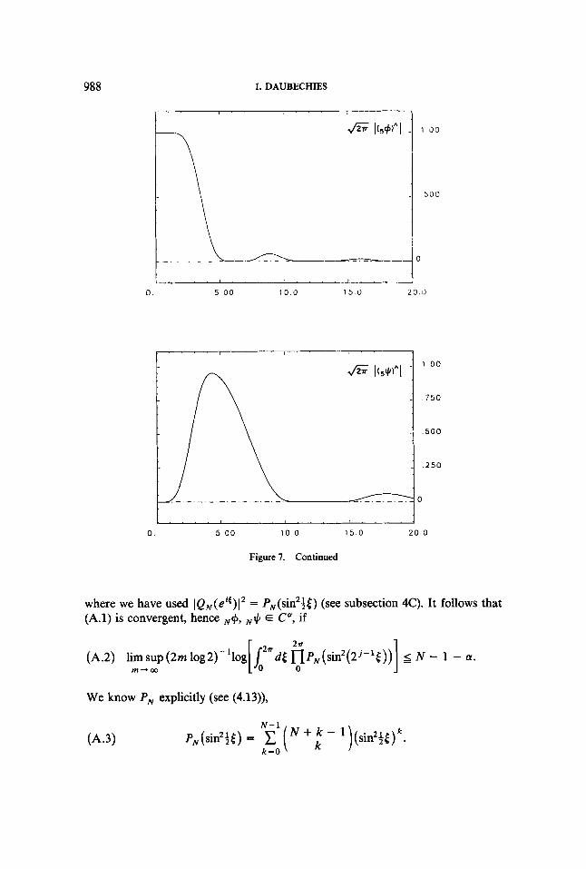
988 I. DAUBECHIES
1 0 0
500
0. 5 00 10 0 15 0 2 0 0
1 00
750
5 0 0
, 2 5 0
0
0 . 5 .00 10 .0 1 5 . 0 2 0 . 0
Figure 7. Continued
where we have used lQN(eit)I2 = PN(sin2+E) (see subsection 4C). It follows that (A.l) is convergent, hence N+, N I c / E C", if
(A.2) limsup (2m log2)-'log[ i 2 % d t @PN(sin2(2j-'t))] 5 N - 1 - a.
We know PN explicitly (see (4.13)),
m-co
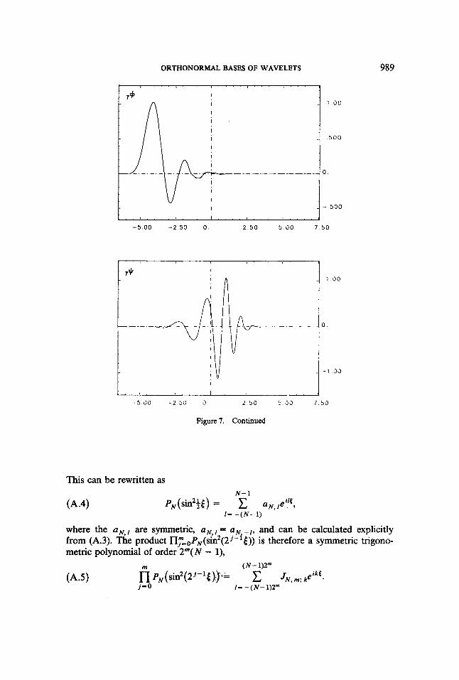
ORTHONORMAL BASES OF WAVELETS 989
1 . " ' " ' ' "
I - 1 0 0
- 500
0
I - - 500
I . . , . ! . . . f . . . . J
-500 - 2 50 0 2 50 5 0 0 7 5 0
This can be rewritten as
where the uN,, are symmetric, a from (A.3). The product II;!,,PN(sin ( metric polynomial of order 2"(N - l),
= uN -,, and can be calculated explicitly 6)) is therefore a symmetric trigono- NJ, i - i
m (N- 1)2" n ~ ~ ( s i n ~ ( 2 j - ' t ) ) ' = c J ~ , , , ; keikE. j-0 I - -(N- 1)2"
(A.5)
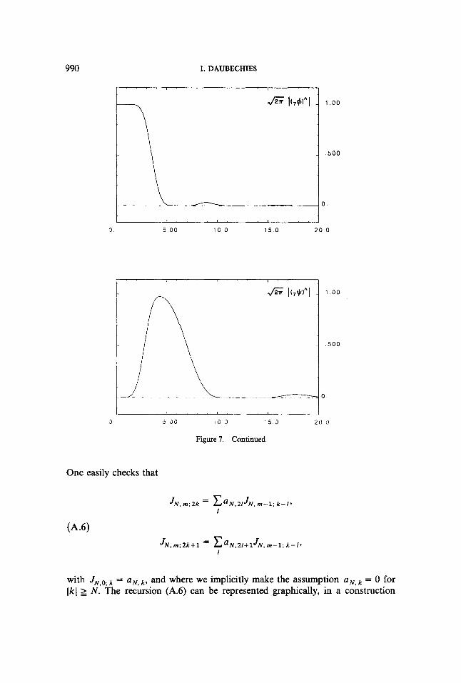
990
Jz 1(7JllAl -
-
I. DAUBECHIES
1 0 0
5 0 0
0
0 5 0 0 10 0 15 0 20 0
One easily checks that
J N , m ; 2 k = ~ a N , 2 1 J N , m - l ; k - 1 , I
- J N , m ; 2 k + l - C a N , 2 1 + l J N , m - l ; k-13
I
with JN,@ k = a N , k , and where we implicitly make the assumption aN, k = 0 for Ikl 2 N . The recursion (A.6) can be represented graphically, in a construction

ORTHONORMAL BASES OF WAVELETS
-~ . I !d 1 0 0
991
Figure I. Continued
analogous to Figure 1. At level 0 we start with JN,?; each successive JN,n is calculated from JN,n-l by a tree algorithm (see Figure 8). To evaluate the left-hand side of (A.2) we need to compute
One can check directly from the recursion (A@, or one can verify on the graphical representation (see Figure 8b) that only the JN, ,,,; ,, 0 5 m' < m, with 111 N - 2 play a role in the computation of JN, m;O. Define d , = 2N - 3. Then
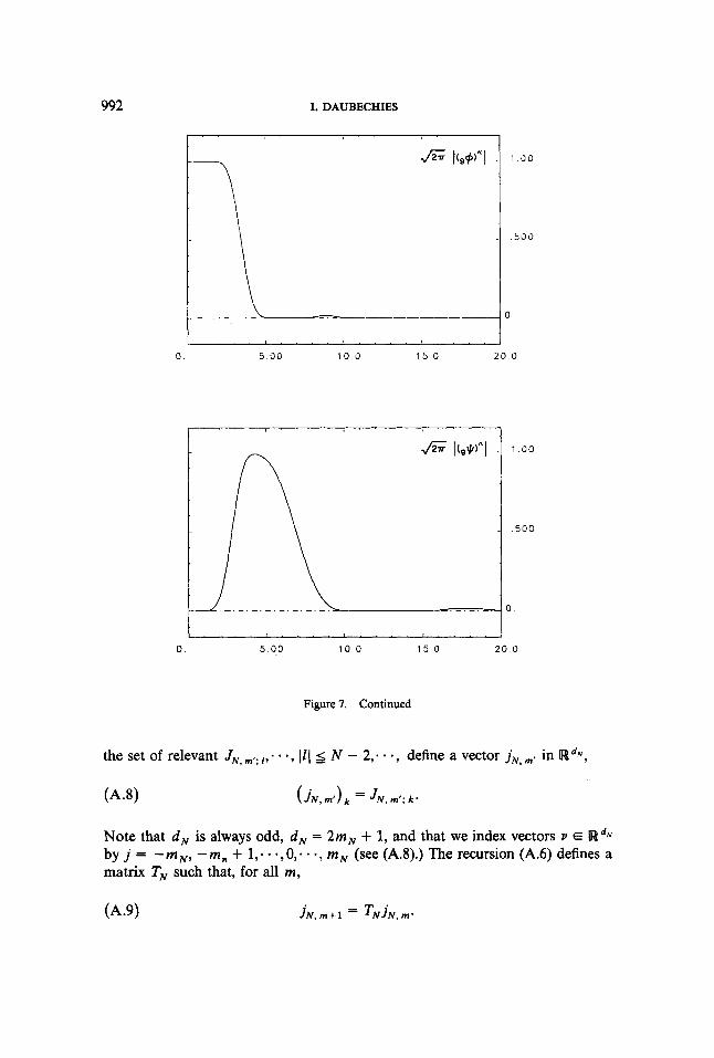
992
f i 1(9qt1)A1 -
-
I. DAUBECHIES
1 0 0
500
0
0 5 0 0 10 0 1 5 0 20 0
Figure I. Continued
the set of relevant J N , mJ; ,,a * ., (11 N - 2, . - *, define a vector JN, mt in R d N ,
( A 4 ( j N , m'>k = JN, m'; k *
Note that d, is always odd, d, = 2mN + 1, and that we index vectors v E R d N
by j = - m N , - m , + 1, * - *, 0, * * - , m (see (A.8).) The recursion (A.6) defines a matrix TN such that, for all m ,
(A.9) j N , m + l = ' N J N , m .
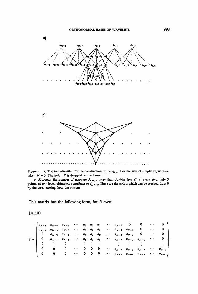
ORTHONORMAL BASES OF WAVELETS 993
. . . . . . . . . .
. . . . . . . . . . . . . . . . . . . . . .
Figure 8. a. The tree algorithm for the construction of the JN, m. For the sake of simplicity, we have taken N = 3. The index N is dropped on the figure.
b. Although the number of non-zero 4, m; more than doubles (see a)) at eve3 step, only 3 points, at any level, ultimately contribute to 4, m; o. These are the points which can be reached from 0 by the tree, starting from the bottom.
This matrix has the following form, for N even:
(A.lO)
T -
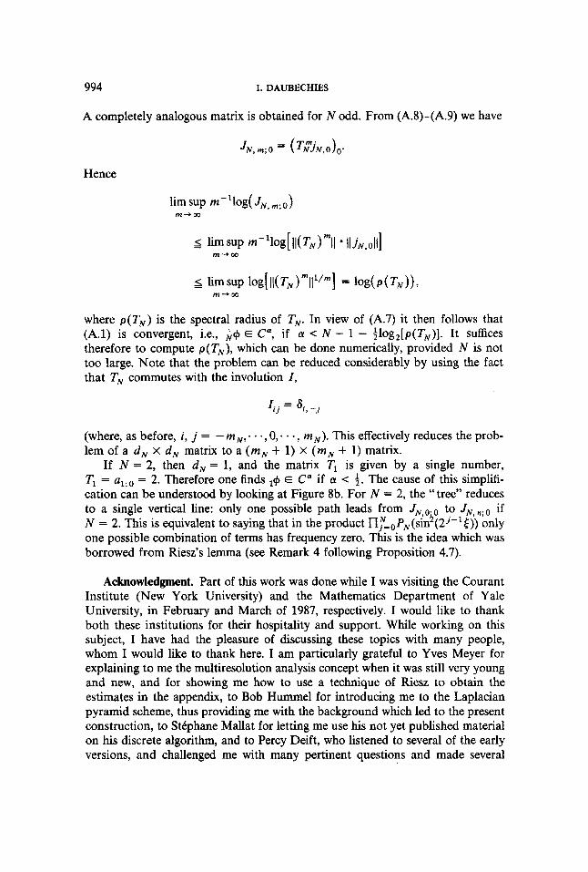
994 I. DAUBECHIES
A completely analogous matrix is obtained for N odd. From (A.8)-(A.9) we have
JN,m;O = (TtjN,o)o.
Hence
limsup m-llog(JN,m;o) m - r m
where p(T,) is the spectral radius of TN. In view of (A.7) it then follows that (A.l) is convergent, i.e., ;+ E Ca, if a < N - 1 - $log,[p(T,)]. It suffices therefore to compute p(T,), which can be done numerically, provided N is not too large. Note that the problem can be reduced considerably by using the fact that T, commutes with the involution I,
I.. = ai, - j ' I
(where, as before, i , j = - mN,- * a , 0,. + -, m,). This effectively reduces the prob- lem of a d , x d , matrix to a (m, + 1) x (m, + I) matrix.
If N = 2, then d , = 1, and the matrix TI is given by a single number, Tl = alio = 2. Therefore one finds E C" if a < 3. The cause of this simplifi- cation can be understood by looking at Figure 8b. For N = 2, the "tree" reduces to a single vertical line: only one possible path leads from JN,o. to J,, n; if N = 2. This is equivalent to saying that in the product Il~-oPN(sin'(2~-1~)) only one possible combination of terms has frequency zero. This is the idea which was borrowed from Riesz's lemma (see Remark 4 following Proposition 4.7).
Acknowledgment. Part of this work was done while I was visiting the Courant Institute (New York University) and the Mathematics Department of Yale University, in February and March of 1987, respectively. I would like to thank both these institutions for their hospitality and support. While working on this subject, I have had the pleasure of discussing these topics with many people, whom I would like to thank here. I am particularly grateful to Yves Meyer for explaining to me the multiresolution analysis concept when it was still very young and new, and for showing me how to use a technique of Riesz to obtain the estimates in the appendix, to Bob Hummel for introducing me to the Laplacian pyramid scheme, thus providing me with the background which led to the present construction, to Stkphane Mallat for letting me use his not yet published material on his discrete algorithm, and to Percy Deift, who listened to several of the early versions, and challenged me with many pertinent questions and made several
ORTHONORMAL BASES OF WAVELETS 995
useful suggestions. I also would like to thank R. Coifman, P. Jones and T. Steeger for their enthusiastic support and for suggesting various references.
The author is “Bevoegdverklaard Navorser” at the Belgium National Science Foundation (on leave). Part of the work for thls paper was done at the Depart- ment of Theoretical Physics, Vrije Universiteit, Brussel from which she also is on leave. She would like to thank both institutions for their support.
Bibliography
[l] Grossman, A., and Morlet, J., Decomposition of Hardy functions into square integrable wavelets of constant shape, SIAM J. Math. Anal. 15,1984, pp. 723-736. Goupillaud, P., Grossmann, A., and Morlet, J., Cyclo-octave and related transforms in seismic signal analysis, Geoexploration 23,1984, 85. The “continuous wavelet transform” is implicitly used in Calderbn, A. P., Intermediate spaces and interpolation, the complex method, Studia Math. 24, 1964, pp. 113-190; see also Calderbn, A. P., and Torchinsky, A., Parabolic maximal functions associated to a distribution, I, Adv. Math. 16,1974, pp. 1-64.
[3] Wilson, K. G., and Kogut, J. B., Physics Reports 12C, 1974, p. 77. Glimm, J., and Jafl‘e, A., Quantum Physics: a Functional Integral Point of View, Springer, New York, 1981.
[4] Meyer, Y., Principe d ’incertitude, bases hilbertiennes et alg6bres d ’opirateurs, Sminaire Bourbaki, 1985-1986, nr. 662.
[Sa] Tchamitchian, P., Calcul symbolique sur les opirateurs de Calderhn-Zygmund et bases incondition- nelles de L2(R”) , C. R. Acad. Sc. Paris. 303, skrie 1, 1986, pp. 215-218.
[5b] Tchamitchian, P., Biorthogonalitt et thtorie des opirateurs, to be published in Rev. Mat.
[2]
Iberoamericana. Battle, G., and Federbush, P., Ondelettes andphase cell cluster expansions; a vindication, Comm. Math. Phys., 1987. Federbush, P., Quantum jeld theory in ninety minutes, Bull. Am. Math. Soc. 17, 1987, pp.
Kronland-Martinet, R., Morlet, J., and Grossmann, A., Analysis of sound patterns through wavelet transforms, to be published in International Journal on Pattern Analysis and Artificial Intelligence. Mallat, S., A theory for mdtiresolution signal decomposition: the wavelet transform, Preprint GRASP Lab, Dept. of Computer and Information Science, Univ. of Pennsylvania, to be published. Grossmann, A., Wavelet transforms and edge detection, to be published in Stochastic Processes in Physics and Engineering (Ph. Blanchard, L. Streit and M. Hasewinkel, eds.), Grossmann, A., Holschneider, M., Kronland-Martinet, R., and Morlet, J., Detection of abrupt changes in sound signals with the heh of wavelet transforms, Preprint, Centre de Physique Thkorique, CNRS, Marseille (France). Grossmann, A., Morlet, J., and Paul, T., Transforms associated to square integrable group representations, I . J. Math. Phys. 26, 1985, pp. 2473-2479; -11: Examples, Ann. Inst. H.
Aslaksen, E. W., and Klauder, J. R., Unitary representations of the afine group, J. Math. Phys. 9, 1968, pp. 206-211; Continuous representation theory wing the afine group, J. Math. Phys. 10,
Paul, T., Functions analytic on the half-plane as quantum mechanical states, J. Math. Phys. 25,
Paul, T., Aflne coherent states and the radial Schriidinger equation. I. Radial harmonic oscillator and hydrogen atom, to be published. Grossmann, A., and Kronland, R., Private demonstration.
93-103.
P0incar6 45,1986, pp. 293-309.
1969, pp. 2267-2275.
1985, pp. 3252-3263.
996 I. DAUBECHIES
[14] Daubechies, I., Grossmann, A,, and Meyer. Y., Painless non-orthogonal expansions, J. Math.
[15] Daubechies, I., The wavelet transform, time-frequency localization and signal analysis, Preprint AT & T Bell Laboratories; to be published.
[16] Meyer, Y., Ondelettes et functions splines, Seminaire EDP, Ecole Polytechnique, Paris, France, December, 1986.
[17] Lemari6, P. G., Ondelettes d localisation exponentielle, to be published, in Journ. de Math. Pures et Appl.
[l8] Battle, G., A block spin construction of ondelettes, Part I: Lemarik functions, Comm. Math. Phys. 1987.
[19] Mallat, S., Multiresolution approximation and wavelets. Preprint GRASP Lab., Dept. of Com- puter and Information Science, Univ. of Pennsylvania, to be published.
[2Oa] Burt, P., and Adelson, E., m e Luplacian pyramid as a compact image code, IEEE Trans. Comm.
[2Ob] Burt, P., and Adelson, E., A multiresolution spline with application to image mosaics, ACM
Phys. 27, 1986, pp. 1271-1283.
31,1983, pp. 482-540.
Trans. on Graphics, 2,1983, pp. 217-236. Jdard, S., Lemarii, P. G., Mallat, S., and Meyer, Y., Multiscale analysis, unpublished memorandum. Coifman, R., and Meyer, Y., 7%e discrete wavelet transform, preprint. Dept. of Math., Yale University. Lemarii, P. G., and Meyer, Y., Ondelettes et bases hilbertiennes, Rev. Mat. Iberomericana 2,
Smith, M. J., and Barnwell, T. P., Exact reconstruction techniques for tree-structured subband coders, IEEE Trans. on ASSP 34,1986,434-441. Auscher, P., These de Doctorat, Universiti de Paris-Dauphine 1988. Rioul, O., private communication. Polya, G., and !beg& G., Aufgaben and Lehrsiitre aus der Analysis, Vol. 11, Springer, Berlin, 1971. Meyer, Y., Wavelets with compact support, Zygmund Lectures (University of Chicago) May 1987, and private communication. Deslauriers, G., and Dubuc, S., Interpolation dyodiqw, in Fractals; Dimensions non EntiJres et Applications, ed. G. Cherbit, Masson (Paris), 1987, pp. 44-45. See also other references listed there. Daubechies, I., and Lagarias, J., Two-scale difference equations. I. Global regularity of solutions, and -. 11. Infinite matrix products, local regularity and fractals, Preprints AT&T Bell Laboratories; to be published.
1986, pp. 1-18.
Received December, 1987


![Image Separation usingWavelets and Shearlets · In [9], a comprehensive theory of compactly supported shearlet frames is provided, i.e., systems with excellent spatial localization.](https://static.fdocuments.in/doc/165x107/5f8ee2278c22d7652848fd97/image-separation-usingwavelets-and-shearlets-in-9-a-comprehensive-theory-of-compactly.jpg)