Working Notes of the AIMDM'99 Workshop on

Prognostic Models in Medicine:

Articial Intelligence and Decision Analytic Approaches

held during

The Joint European Conference on Articial Intelligence

in Medicine and Medical Decision Making, AIMDM'99

Aalborg, Denmark, 20 June, 1999

Ameen Abu-Hanna & Peter Lucas (editors)

Preface

These are the working notes of the workshop on Prognostic Models in Medicine: Ar-

tificial Intelligence and Decision Analytic Approaches, which was held during the

Joint European Conference on Articial Intelligence in Medicine and Medical Decision Mak-

ing, AIMDM'99, on 20 June, 1999, in Aalborg, Denmark. This workshop brought together

various theoretical and practical approaches to prognosis that comprise the state of the art

in this eld. It is a follow-up on a very successful invited session on Intelligent Prognos-

tic Methods in Medical Diagnosis and Treatment Planning during the conference

Computational Engineering in Systems Applications 1998 (CESA'98). AIMDM'99 joined the

research elds of Medical Articial Intelligence and Medical Decision Analysis. One of the

aims of the present workshop was, therefore, to combine the views of researchers from these

two dierent, although related, elds as well. This is not only re ected in the title of theworkshop, but also in the contributions to it as contained in the working notes.

Prognostic models are increasingly used in medicine to predict the natural course of dis-

ease, or the expected outcome after treatment. In evaluating quality of care, prognostic

models are used for predicting outcome, such as mortality, which may be compared with

the actual measured outcome. Furthermore, prognostic models may play a role in guiding

diagnostic problem solving, e.g. by only requesting information concerning tests, of which the

outcome aects knowledge of the prognosis.

Various methods have been suggested in Medical Articial Intelligence for the representa-

tions of prognostic models ranging from quantitative approaches, such as Bayesian networks

and neural networks, to symbolic and qualitative ones, such as decision trees, as proposed

within the machine-learning community. Dealing with semantic concepts such as time hasbeen, and still is, a challenging issue. Temporal Bayesian networks and in uence diagrams,

and Markov decision processes have been developed as formalisms to deal with time explicitly.

Similarly, in Medical Decision Analysis various representations with underlying techniques are

suggested, such as decision trees, regression models, and representations in which advantage

is taken from the Markov assumption. Hence, it is not easy to decide which representation

formalism to choose to develop a specic prognostic model. The present working notes shed

some light on this diÆcult issue, and oer a lot of useful practical experience in model building

as well.

We are grateful to our colleagues who served on the programme committee of the workshop

on Prognostic Models in Medicine (members are: A. Abu-Hanna (co-chair), S.S. Anand,

S. Andreassen, P.M.M. Bossuyt, J. Fox, L.C. van der Gaag, J.D.F. Habbema, P. Haddawy,P. Hammond, E. Keravnou, N. Lavrac, J. van der Lei, P.J.F. Lucas (co-chair), L. Ohno-

Machado, M. Ramoni, M. Stefanelli, Th. Wetter, J. Wyatt). They have carefully read and

reviewed each submission until the acceptance of the nal papers. Thanks are also due to Dik

Habbema, Kristian Olesen and Jeremy Wyatt for accepting to give the three invited talks of

the workshop.

Ameen Abu-Hanna, Department of Medical Informatics, University of Amsterdam

Peter Lucas, Department of Computer Science, Utrecht University

6 June, 1999

i

ii

Contents

Preface i

Invited Talks 1J.D.F. Habbema: Building Prognostic Models: Statistical Aspects . . . . . . 3

K.G. Olesen: Medical Models and Bayesian Networks . . . . . . . . . . . . . 5

J. Wyatt: Prognostic Models in Medicine . . . . . . . . . . . . . . . . . . . . 7

Papers 9P.J.F. Lucas and A. Abu-Hanna: Prognostic Models in Medicine . . . . . . . 11

S.S. Anand, P.W. Hamilton, J.G. Hughes and D.A. Bell: Utilising Censored

Neighbours in Prognostication . . . . . . . . . . . . . . . . . . . . . . . 15

S. Antel, L.M. Li, F. Cendes, Z. Caramanos, A. Olivier, F. Andermann, F.

Dubeau, R.E. Kearney, R. Shinghai, D.L. Arnold: A Naive Bayesian

Classier for the Prediction of Surgical Outcome in Patients with Tem-

poral Lobe Epilepsy . . . . . . . . . . . . . . . . . . . . . . . . . . . . . 21

H. Dreau, I. Colombet, P. Degoulet, G. Chatellieri: Identication of Patients

at High Cardiovascular Risk using a Critical Appraisal of Statistical Risk

Prediction Models . . . . . . . . . . . . . . . . . . . . . . . . . . . . . . 27

L. Ohno-Machado and S. Vinterbo: In uential Case Detection in Medical

Prognosis . . . . . . . . . . . . . . . . . . . . . . . . . . . . . . . . . . 33

N. Peek: A Specialised POMDP Form and Algorithm for Clinical Patient

Management . . . . . . . . . . . . . . . . . . . . . . . . . . . . . . . . . 39

M. Ramoni, P. Sebastian and R. Dybowski: Robust Outcome Prediction for

Intensive-care Patients . . . . . . . . . . . . . . . . . . . . . . . . . . . 45

R. Schmidt, B. Pollwein and L. Gierl: Prognoses for multiparametric time

course of the kidney function . . . . . . . . . . . . . . . . . . . . . . . . 51

I. Zelic, N. Lavrac, P. Najdenov, Z. Rener-Primec: Impact of Machine Learn-

ing to the Diagnosis and Prognosis of First Cerebral Paroxysm . . . . . 57

iii

Invited Talks

Building Prognostic Models:

statistical aspects

Dik Habbema & Ewout Steyerberg

Department of Public Health

Medical Faculty, Erasmus University Rotterdam

P.O. Box 1738, 3000 DR Rotterdam, The Netherlands

Email: habbema@mgz.fgg.eur.nl

Prediction is a crucial activity in clinical medicine. Sometimes it deals with the unknown

future; in this case we want to predict the outcome for patients (`prognosis'). Alternatively,

prediction concerns the present, namely prediction of disease condition or diagnosis (the

`pre-' in prediction refers here to `before you know'). We will use the terms predictors and

outcome for the statistical variables involved; alternative names are explanatory variables and

explicandum, or independent variables and dependent variable etc.

Two issues will be addressed:

Which predictors to use?

How to measure the performance of the prediction rule?

Which predictors to use? We will question the general usefulness of trying to select a few

predictors out of a larger number available predictors. Recent results indicate that classical

statistical forward or backward selection procedures have been used with too much enthusi-

asm. Problems will be discussed, and illustrated with examples. Sample size is important,

and cautiousness is especially indicated for small samples. A closely connected question is

what importance to attach to the selected versus the non-selected predictors. Here a lot of

confusion exists, and we as methodologists may have been too lazy with explaining to clini-

cians that there may be a high degree of arbitrariness in the result of the selection process,

and that further inspection is needed before equating `selection' to `importance'.This will again be discussed using examples, and some emphasized on analyzing the struc-

ture of the mutual dependency between the predictors, and the dependency between predictors

and predictor.

Performance measurement, which is also relevant for the selection of predictors issue, will

be taken further. A well known fundamental observation is that a too favorable impression

of performance is obtained when it is measured on the same patients as have been used for

the construction of the prediction model. There are two main approaches to more realistic

estimation of regression coeÆcients and performance measurement: a simulation approach

using bootstrap re-sampling and a formula-based direct shrinkage of regression coeÆcients.

In large samples, split sample may also be used: although this method is easily understandable

to clinicians,we should realize that information will be thrown away.Finally, some remarks will be made on dierences between exploratory, explanatory and

predictive use of the type of models as discussed. It is argued that the basic process will

remain the same under these three uses, but emphasis and detail may dier considerably.When clinical use of the prediction model is aimed at, the costs of measuring the predictors

have to be taken into account, at least when they have no other clinical relevance than their

use in the prediction model.

Medical Models and Bayesian Networks

Kristian G. Olesen

Department of Computer Science, Aalborg UniversityFrederik Bajers Vej 7, DK-9220 Aalborg , Denmark

Email: kgo@cs.auc.dk

The use of computers in health care has increased dramatically over the past decades and com-

puters are now involved in practically all tasks in the sector, including patient management,

communication, diagnosing, planning of theraphy and test, prognosis, and quality control.

The rst two tasks mentioned in the list are well understood and reliable computer support

for them exists. The remaining tasks are more complicated and, in general, characterized by

inherent uncertainty, and this makes it diÆcult to construct generally accepted automated

tools to support them. It is important that such systems are transparent and that they meet

their users on the users premises. Models based on the concepts usually used by physisians

are preferred and such models should exhibit the structure of the domain in question through

explicit representation of the relations between concepts. This enables a scientic discussion

of the model itself independent of its use, thereby making it transparent and open for criti-

cism. Moreover, such models should be powerful enough to support procedures for a variety

of tasks. Bayesian networks oer a framework in which such models can be constructed.

This talk will present the basics of Bayesian networks and illustrate their use through a

number of examples. The basic structure of a Bayesian network model consists of a graph

where the nodes are stochastic variables modelling the concepts of a domain. The edges of the

graph models direct dependencies between variables and the strength of these dependencies

are quantied by conditional probability distributions. Bayesian networks represent the joint

probability distribution over all variables in the domain and this distribution can be updated

dynamically as evidence arrives. This makes Bayesian networks suited for diagnostic systems

where the current belief in a set of disorders can be maintained, thereby representing the

basis for decisions.

The planning of tests and therapy involve active decisions, where the state of the world

is in uenced. These tasks can be integrated in the Bayesian network formalism through

the addition of decision and utility nodes. Such extended models are known as in uence

diagrams. Decision nodes are under the full control of the decision maker and utility nodes

are real-valued functions used to model the decision makers preferences. Optimal decisions

are then computed by maximizing the expected utility.

Prognostic Models in Medicine

J.C. Wyatt

School of Public PolicyUniversity College London29/30 Tavistock SquareLondon, WC1H 9EZ, UK

Papers

Prognostic Models in Medicine:Articial Intelligence and Decision Analytic Approaches

Peter Lucas

Department of Computer Science

Utrecht University, PO Box 80089

3508 TB Utrecht, The Netherlands

E-mail: lucas@cs.uu.nl

Ameen Abu-Hanna

Department of Medical Informatics

AMC-UvA, Meibergdreef 15

1105 AZ Amsterdam, The Netherlands

E-mail: a.abu-hanna@amc.uva.nl

Abstract

This paper is meant as an introduction to theworkshop on Prognostic Models in Medicine:Articial Intelligence and Decision AnalyticApproaches held during aimdm'99. Prog-nosis the prediction of the course andoutcome of disease processes, either or notchanged due to interventions is an impor-tant aspect of medical tasks like diagnosisand treatment management. Techniques forbuilding prognostic models vary from tra-ditional probabilistic approaches, originat-ing from the eld of statistics, as used indecision analysis, to more qualitative andmodel-based approaches originating from theeld of articial intelligence. The workshopbrings these two elds of research togetherin the hope that a fruitful exchange in ideaswill take place.

1 Introduction

Prognosis, the prediction of the course and outcomeof disease, is a subject that lies at the heart of pa-tient management. There is little sense in delving intothe cause of particular symptoms and signs in a pa-tient, and to initiate elaborate diagnostic procedures,if it is known beforehand that no eective treatmentof the considered disease exists. Furthermore, alsotreatment selection invariably involves taking possi-ble future benecial and harmful eects into account,i.e. prognostic information [4].Of course, the process of patient management con-

cerns issues other than prognosis as well. The primaryrole of the physician is to guide the patient throughthe disease process, which involves much more thanprognostication. Even the processes of diagnosis andtreatment selection may be seen in this light of guid-ance of patients. This view may explain why progno-sis, despite its central role in medicine, is not clearlyrecognised as such in typical medical textbooks, likeHarrison's Principles of Internal Medicine [1]. Thesubject of prognosis is only paid attention to when itis obviously important, such as in cancer treatment.

It is likely that this situation will change in thenear future, and that the role of prognostic models inmedicine will increase. Medicine as a eld is becom-ing increasingly complex, as is re ected by the annu-ally increasing number of dierent diagnostic tests andtherapies from which a clinician must choose. Prog-nostic models are required to guide clinicians in thisselection process to ensure that the patient will benetfrom further progress in medical science.

2 Prognostic models

As has been said above, there are a number of eldsin medicine, where prognostic models are of particu-lar importance. Examples of such elds are: oncol-ogy, transplantation medicine, and trauma medicine.Usually, prognostic models focus either on long-termor short-term eects. For example, long-term ef-fects dominate in treatment considerations in oncol-ogy, whereas short-term eects are more signicant intrauma medicine. Adequate prognostic information isof major importance in these elds so that prognosticmodels of various kinds, not necessarily mathemati-cal in nature, have been in use for quite some time.Often these models are coarse and lack detail. TheTNM staging system that is used to assess a primarymalignant tumour in terms of its size (indicated by T0

to T4, where an increase in subscript corresponds toan increase in tumour size, as dened for a particu-lar type of tumour), regional lymph node involvement(N, also supplied with a subscript), and presence ofdistant metastatis (M) is an example of a simple qual-itative tool to assess prognosis in cancer patients. An-other example is the Apache III scoring system, whichis based on a logistic regression model, and that hasbeen shown to have a good predictive ability for pa-tients with severe illness, and for a large variety ofdiseases [2].As one may expect, clinicians are only prepared to

accept prognostic models when it is obviously thatthey will contribute to quality of care [7]. Prognosticmodels are not only used in a clinical setting. Theyare also used, and may even have had a larger impact,in the design of clinical trials, counselling patients andin medical technology assessment.

In general, and independent of particular applica-tions of prognostic models, the problem of the de-sign of accurate prognostic models is the capturing ofthe many possible subtle interactions among variablesthat exist. It is largely determined by the (mathe-matical) modelling tools used to what extent such in-teractions can be represented, and learnt from data,possibly augmented with background knowledge.

3 Articial intelligence and decision

analysis

Medical articial intelligence is generally concernedwith the development of medical models for variouspurposes, but usually the aim is to assist cliniciansin the processes of diagnosis, treatment or prognosisof diseases in patients. A key characteristic is theexplicit representation of the medical knowledge in-volved, i.e. the explicit representation of meaningfulinteractions among the factors that play a role in aparticular medical problem is favoured [3]. However,there are a number elds in articial intelligence, suchas neural networks, where the goal of explicit represen-tation is less dominant. There is now an entire arrayof dierent techniques from which medical AI practi-tioners may choose. One of the diÆcult problems hasbeen the representation of temporal patterns, whichis now addressed by a number of dierent formalisms.Progress in the eld has yielded new, exible tech-niques, like Bayesian networks, neural networks andgenetic algorithms; these oer new opportunities fordealing with the issue of prognostication.

Medical decision analysis oers a systematic ap-proach to medical decision making under conditions ofuncertainty [5; 6]. It has studied the use of prognos-tic models in the process of decision making for morethan two decades. An enormous amount of practicalexperience in building medical models has been builtup during these years. However, there has been littleprogress in the eld with respect to new techniquesand tools that may be used to carry out a decisionanalysis.

Until recently the elds of medical articial intelli-gence and decision analysis appeared to have only incommon that in both model building is of crucial im-portance. In the eld of articial intelligence there hasbeen a revival of interest in numerical methods stem-ming from probability and decision theory, and fromthe eld of neural networks. The new ideas and tech-niques that have come out of this, has not passed byunnoticed by the medical decision analysis community.There currently seem to be much interest in that eldwith respect to applicability of these technique. At thesame time, medical articial-intelligence researchersrealise that much can be learnt from the more matureeld of medical decision analysis. This workshop istherefore a timely opportunity to exchange ideas andhopefully to learn from each other.

4 Road-map to the workshop papers

To conclude this introductory paper, we shall brie ysummarise the contents of the papers in the workingnotes.The paper by S.S. Anand, P.W. Hamilton, J.G.

Hughes and D.A. Bell, titled Utilising censored neigh-bours in prognostication, discusses an extended versionof the k-nearest neighbour algorithm, which is appliedto the problem of prediction of the survival of patientswith colorectal cancer. Novel is the possibility of deal-ing with censored patients, which is typically requiredin survival analysis in medicine. The paper by S. An-tel, L.M. Li, F. Cendes, Z. Caramanos, A. Olivier, F.Andermann, F. Dubeau, R.E. Kearney, R. Shinghaiand D.L. Arnold, with title A naive Bayesian classi-er for the prediction of surgical outcome in patientswith temporal lobe epilepsy, focusses on a number ofimportant issues that arise when one wants to developprognostic models the are clinically useful. The devel-opment of a Bayesian classier for the prediction of theoutcome of patients with temporal lobe epilepsy thatundergo surgery is reported. Bayesian classiers arealso the topic of the paper Robust outcome predictionfor intensive-care patients byM. Ramoni, P. Sebastianand R. Dybowski, but here the main issue is how todeal with missing values in clinical data. A compar-ison is made between logistic regresssion augmentedwith an imputation mechanism and what is called arobust Bayesian classier in which no assumptions aremade with respect to the mechanisms underlying miss-ing data.In the paper by H. Dreau, I. Colombet, P. Degoulet,

G. Chatellieri, titled Identication of patients at highcardiovascular risk using a critical appraisal of statis-tical risk prediction models not techniques, but dif-ferent statistical risk-prediction models are compared.This paper sheds light on the assumptions underlyingstatistical models, and on the question to which extentassumptions are valid and may aect the conclusionsthat may be drawn.There are a number of papers in which statistical

or decision-analytic techniques are compared or com-bined with AI techniques. For example in the paperby L. Ohno-Machado and S. Vinterbo, In uential casedetection in medical prognosis it is studied whether agenetic algorithm oers advantages over conventionaltechniques for the selection of cases in the construc-tion of prognostic logistic regression models. The pre-diction of the prognosis of trauma patients has beenchosen as an example domain. I. Zelic, N. Lavrac, P.Najdenov and Z. Rener-Prime in their paper Impactof machine learning to the diagnosis and prognosis ofrst cerebral paroxysm compare ID3-like decision-treeinduction with naive Bayesian classiers from the per-spective of machine learning. The comparison is car-ried out in the medical domain of epilepsy.The remaining two papers focus on medical applica-

tions of techniques from the areas of articial intelli-gence. In the paper by N. Peek, A specialised POMDP

form and algorithm for clinical patient managementthe formalism of partially observable Markov decisionproblems (POMDPs) is studied. This formalism hasoriginally been introduced in articial intelligence as ameans to handle planning problems under conditionsof uncertainty. POMDPs, however, have also beensuggested as a suitable formalism for medical treat-ment planning. Since the formalism is known to beintractable in general, this papers proposes the useof Monte Carlo simulation to render the formalismpractically more useful. The paper by R. Schmidt,B. Pollwein and L. Gierl, titled Prognoses for mul-tiparametric time course of the kidney function alsodiscusses the suitability of a technique from the eldof articial intelligence to the development of prog-nostic models, namely the application of case-basedreasoning to the prediction of kidney function. Ad-vantages and limitations of case-based reasoning areclearly discussed.We may conclude that the papers in the workshop,

although all dealing with the issue of prognostic mo-cels, are indeed varied; both methods and techniquesfrom the elds of articial intelligence, decision anal-ysis and statistics are covered by the papers. Some-times these techniques are dealt with separately, some-times they are combined and in some papers they arecompared to each other. It may therefore be con-cluded that the title of the workshop does indeed re- ect the contents of the papers in the workshop notes.

References

[1] K.J. Isselbacher, et al., Harrison's Principles ofInternal Medicine, 13th edition, McGraw-Hill,New-York, 1994.

[2] W.A. Knaus, E.A. Draper, J. Lynn, Short-termmorbidity predictions for critically ill hospitalisedpatients science and ethics, Science 254 (1991)38994.

[3] P.J.F. Lucas, Logic engineering in medicine, TheKnowledge Engineering Review, Vol. 10, No. 2,1995, pp. 153179.

[4] P.J.F. Lucas and A. Abu-Hanna, Prognosticmethods in medicine. Articial Intelligence inMedicine, vol. 15, 1999, pp. 105119.

[5] H.C. Sox, M.A. Blatt, M.C. Higgins, K.I. Marton,Medical Decision Making, Butterworths, Boston,1988.

[6] M.C. Weinstein and H.V. Fineberg, Clinical De-cision Analysis, W.B. Saunders, Philadelphia,1980.

[7] J.C. Wyatt and D.G. Altman, Commentary prognostic models: clinically useful or quickly for-gotten, BMJ, Vol. 311, 1995, pp. 15391541.

AbstractEvaluation of new modelling techniques is anessential part of their development and accep-tance within the medical domain. The modelsdeveloped need to be evaluated along a numberof dimensions - accuracy of the resulting model,perspicuity of the model, its ability to handledomain knowledge, its ability to handle dataspecific characteristics and its ability to continu-ally refine the model. Feedback from suchevaluations must be used to enhance presentmodelling techniques. In this paper we extendthe basic k-nearest neighbour (k-NN) paradigm,based on an earlier evaluation [Anand et al.,1999], so as to enhance its capabilities with re-spect to handling censored patient data. We referto this new k-NN algorithm as Censored k-NN(Ck-NN). Two aspects of the k-NN are ex-tended, the distance metric, used to retrieve thenearest neighbours of a target case, and the pre-diction mechanism used to provide a point esti-mate for the dependent attribute. Ck-NN isevaluated by using it to model survival time forcolorectal cancer patients.

1 IntroductionPrognostic models have traditionally been developed usingmethods from medical statistics that have been developed tohandle complexities within medical data. Censored observa-tions are only one such aspect of medical data that makemodelling more complex. Statistical techniques such asCox’s regression, Kaplan-Meier and Weibull modelling[Collett, 1994] deal with such data.

It is our belief that new techniques used to build prog-nostic models, just as in the case of any other form ofdecision support system in medicine, must provide addi-tionality - net added benefits - over these traditional,established techniques if they are to find large-scale ac-ceptance within the medical domain. In general, addi-tionality must be measured along a number of differentdimensions – accuracy of the resulting model, perspicu-ity of the model, its ability to handle domain knowledge,

its ability to handle data-specific characteristics such asskewness of distributions, censored observations etc. andits ability to continually refine the model, providing sup-port for both the generic learning tasks of knowledgeacquisition and knowledge refinement.

In a previous paper, we compared neural networks, re-gression tree induction, linear regression, Cox’s regres-sion and the nearest neighbour paradigm with the aim ofascertaining their suitability for modelling survival timefor colorectal cancer patients [Anand et al., 1999]. Theconclusions arrived at in that study can be summarised asfollows. Firstly, there is a general lack, in the literature,of evaluation of new AI techniques against tried andtested statistical techniques. Secondly, within the domainaddressed, Cox’s regression and neural networksachieved similar accuracy. However, neural networkswere, in general, unable to handle censored patient data.The work by Farragi and Simon [Faraggi and Simon,1995] is an exception to this rule. With respect to perspi-cuity of the model, both neural networks and Cox’s re-gression are not ideal, as the survival baseline and expo-nential terms in Cox’s model reduce the intuitiveness ofthe interpretation of the model while neural networks areknown to generate a “nervousness” within clinicians[Wyatt, 1995]. In fact, it has been pointed out that re-gression trees that are generally thought of as beingreadily understandable fail to meet another aspect of per-spicuity - intuitiveness [/DYUDþ @ &OLQLFLDQV ILQGregression trees to be less intuitive as they utilise mini-mal “relevant” information as opposed to the informationavailable in its entirety. The nearest neighbour paradigmwas found to be psychologically plausible and under-standable. However, the basic paradigm scored low onthe accuracy scale mainly due to the presence of irrele-vant attributes and the existence of biases within thedistance metric used. Another failing was its inability tohandle censored observations. Enhancements made to thebasic paradigm with respect to the distance metric andattribute weight discovery mechanism, proved to be ef-fective in improving the accuracy of the model. The issueof handling censored data within the nearest neighbourparadigm was only briefly discussed in previous work bythe authors, and is the subject of the present study. More

Utilising Censored Neighbours in Prognostication

Sarabjot S. Anand, John G. Hughes, David A. Bell Peter W. HamiltonSchool of Information and Software Engineering,

University of Ulster at Jordanstown,Newtownabbey, County Antrim

Northern Ireland BT37 0QB

Department of Pathology,Queens University of Belfast,

Northern Ireland

specifically, we investigate how censored observationscan be incorporated into the distance metric and how thecensored and uncensored retrieved nearest neighbourscan be utilised to arrive at a single prediction for the de-pendent attribute of the target example.

2 Incorporating Censored Data withinthe Distance Metric

Traditionally, the k-NN uses the Euclidean and Manhattandistances to compute the distance between the target exam-ple and exemplars within the exemplar base. When some ofthe attributes describing the exemplars are categorical, thesetraditional metrics introduce a bias, into the retrieval of thenearest neighbours, towards matching categorical attributevalues. Anand et al. [Anand and Hughes, 1998] introduced anumber of enhanced distance metrics that remove this biaswhen using the nearest neighbour paradigm for predicting acontinuous valued dependent attribute, such as, survivaltime.

([HPSODU%DVH

([HPSODU%DVH3DUWLWLRQVEDVHGRQ&DWHJRULFDO$WWULEXWH9DOXHV

'HSHQGHQW$WWULEXWH'LVWULEXWLRQV&RQGLWLRQHGRQ&DWHJRULFDO$WWULEXWH9DOXHV

9

9

9

9

9

9

9

9

G9 9

G9 9

&RPSXWDWLRQRI$WWULEXWH'LVWDQFH

Figure 1: Enhanced Distance Metrics for Categorical Attrib-utes

The enhanced distance metrics are based on the followingobservation (Figure 1). A categorical attribute, with domainsay V1, V2, V3, V4, effectively partitions the exemplarbase. Each partition is defined by a unique categorical at-tribute value. We refer to the distribution of the dependentattribute within a partition as the distribution conditioned onthe categorical value defining the partition. Anand et al. de-fine the distance between two categorical attribute values,say d(V1,V2), based on the difference between the resultingdependent attribute distributions conditioned on the valuesof the categorical attribute. The difference between two dis-tributions may be defined by using any of a number of sta-tistical tests, comparing either the central tendency measuresof the two distributions (for example, using the t-test), or thewhole distributions (for example, using the Kolmogorov-Smirnov test).

While such a definition of the distance between categori-cal values has been shown to be effective [Anand et al.,1999], in the presence of censored observations, the ob-served survival time distribution may be quite different fromthe true distribution and the resulting distance metric wouldonce again be biased. In this section we discuss an alterna-

tive definition of the distance between two categorical val-ues, based on the survivor curve, as defined in the Kaplan-Meier model for survival analysis, conditioned on the cate-gorical values. The advantage of using the survivor curvesrather than the survival time distributions is that the survivorcurves take account of censored observations in their defini-tion, whereas the survival time distributions do not do so.

The enhanced metrics defined in [Anand and Hughes,1998] as well as the metrics described in this section can bejustified by the fact that the nearest neighbour assumes inde-pendence of the attributes used to build the model (as in thecase of the naive Bayes methods). Based on the independ-ence assumption the distribution of survival times condi-tioned on a categorical value can be assumed to be unaf-fected by any of the other attributes describing the exemplar.Thus, the Kaplan-Meier based survivor curve definition issufficient. For cases were this does not hold, Kasif et al.suggest a probabilistic framework for the nearest neighbourparadigm that may be employed [Kasif et al., 1998].

The survivor curves corresponding to two different valuesof a categorical attribute (conditional survivor curves) maybe compared in a number of ways. A simplistic method is tocompare the survival time for the two curves at the half-life(i.e. survivor probability of 0.5). Alternatively, more rigor-ous methods of comparison such as the log-rank test andWilcoxon test may be used. We investigate all three meth-ods here.

Figure 2: Survivor curves conditioned on values of VenousInvasion

Figure 2 shows the conditional survivor curves for Ve-nous Invasion using a data set from the colorectal cancerdomain [Anand et al., 1999]. The resulting mapping of thecategorical attribute values onto a numeric scale of [0,1]using the median survival time (i.e. the survival time atprobability 0.5), are shown in Table 1. Table 1 also showsthe mapping of Venous Invasion when using the Mean andCoefficient of Variation as the basis for the mapping dis-cussed previously [Anand and Hughes, 1998]. The mappingonto the [0,1] scale based on the median survival is medi-cally more intuitive than those based on central tendencymeasures of the survival distribution itself. As would beexpected, the distance between no venous invasion and

0

0.2

0.4

0.6

0.8

1

1.2

0 10 20 30 40 50 60 70

Survival Time

Pro

bab

ility

Thinwalled Thickwalled No

thick-walled venous invasion is greater than the distancebetween thin-walled venous invasion and the two extremes.

VenousInvasion

MedianSurvival

MappedValue

MeanBased

Coefficient ofVariation based

No 36 1 1 0.223Thin-walled

31 0.687 0 0

Thick-walled

22 0 0.172 1

Table 1: Mapping of Venous Invasion onto the scale [0,1]

The Log-Rank test and Wilcoxon test are two non-parametric tests that can be used as a more rigorous basis forthe comparison of survivor curves. Both statistics are dis-tributed as the chi-square distribution with one degree offreedom. Thus, the probability, p, that the two curves belongto the same underlying distribution can be obtained using thechi-square distribution. Using the Log-Rank test and Wil-coxon test, the resulting distance matrices, defined as 1-p,are as shown below.

ThinwalledNo 0.211 NoThickwalled 0.818 0.703

Table 2: Distance Matrix for Venous Invasion using the Log-Rank test

ThinwalledNo 0.533 NoThickwalled 0.807 0.855

Table 3: Distance Matrix for Venous Invasion using the Wil-coxon test

In the case of the Log-Rank test the resulting distances donot follow the intuitive expectations as in the case of themedian based and Wilcoxon test based metrics. Further in-vestigation of why this is the case must be undertaken. Onepossible explanation is that the Log-rank test is more sensi-tive to changes in the tail of the left-skewed curves whichmay be causing this anomaly.

3 Predictions based on Censored Pa-tient Data

Using the distance metrics defined in the previous section,the ’k’ nearest neighbours for a given target are retrievedfrom the exemplar base. These exemplars must now be usedto arrive at a single prediction for the target.

In the case of the colorectal cancer data set, all censoredobservations are right censored. Thus, the recorded observedsurvival for the censored observations can be interpreted aslower bounds to the true survival lengths for these patientsand may be modelled within the data as a survival of“greater than <observed value>” (Table 4). In effect, whatwe now have is a complex, structured dependent attributethat needs to be modelled using the existing set of independ-ent attributes. While such an approach is intuitive, few mod-elling techniques can handle such a structured dependentattribute.

Consider the case where k nearest neighbours n1, n2, . . . ,nk have been retrieved from the exemplar base when pre-sented with the target example, t. Let o1, o2, . . . , ok be thedependent attribute values for the k neighbours and d1, d2, . .. , dk be the distances of these k neighbours from the target.Of the k neighbours, let us assume without loss of general-ity, that the first c neighbours are uncensored observationswhile the rest of the k-c neighbours are censored. Now, us-ing the kernel function, K(d), defined below, we can associ-ate a vote with each of the retrieved neighbours denoted byv1, v2, . . . . , vk. The kernel function should associate asmaller vote with neighbours that are further away from thetarget.

Sex

Pat

h T

ype

Pol

arity

Con

figu

ratio

n

Pat

tern

Infi

ltrat

ion

Fib

rosi

s

Ven

ous

Inva

sion

Mito

tic C

ount

Pen

etra

tion

Dif

fere

ntia

tion

Duk

es S

tage

Age

Obs

truc

tion

Site

Surv

ival

M Signet lost simple expanding little little no 0-5 node well A1 34 No rectum > 40F Tubular Easily discerned simple infiltrating marked little no 6-10 serosa poor C 48 No caecum > 22M Signet Easily discerned simple expanding little little yes 0-5 node poor D 78 No caecum 5

Table 4: Example data using “lower bound” interpretation of right censored data

v K d

dd

dd

i i

ij

k

ij

kk

= =

− ∑

− ∑

∑

( )

1

1

The votes v1, v2, . . . . , vc can be used to combine the val-ues of the dependent attribute associated with the c uncen-sored observations using the formula:

o

v o

v

i ii

c

ii

c= =

=

∑

∑

.1

1

with an associated vote v defined as:

v vii

c

==∑

1 .Now, given the definition of the kernel function, it is

straightforward to prove that the kernel function is an evi-dential mass function [Anand et al., 1996]. The function, m,that maps the k-c+1 dependent attribute values onto the in-terval [0,1] representing the evidential mass associated withthat particular value of the dependent attribute being theexpected value may be defined as:

m(oj) = vj ∀ i ∈ [k-c, k]and m(o) = v

Associated with the mass function, a belief function maybe defined as,

where X and Y are subsets of the frame of discernment de-fined as the set of all possible outcome values.

The outcome value with belief greater than and closest to0.5 would be the preferred outcome. The value of 0.5 is thegenerally accepted value used in modelling. In survivalanalysis it is often referred to as the half-life, as it is thepoint at which the probability of the predicted outcome be-ing the true outcome is not less than the probability of thepredicted outcome being incorrect. A more conservativeprediction would be to use a higher threshold value. Thevalue of 0.5 is taken to be a balance between correctness andinformativeness of the predicted value. For example, a pre-diction of “> 0” will always be a correct prediction but itsinformativeness will be the lowest possible.

Neighbour # distancefrom target

dependentattribute value

Vote (usingkernel function)

1 1.4 25 0.2072 1.5 30 0.2043 1.6 > 30 0.2014 1.8 > 40 0.1955 2 > 50 0.189

Table 5: Example retrieved neighbours

We illustrate the prediction mechanism using an example,assuming k to be 5. Table 5 shows the distance for the tar-get, dependent attribute values and votes associated witheach of the five neighbours. In the example, there are threecensored observations within the retrieved set of neighbours.Combining the uncensored observations we get a combined

value of 27.481 and vote of 0.411. The resulting mass func-tion is:m(27.481) = 0.411, m(> 30) = 0.201, m(> 40) = 0.195, m(>50) =0.189.and the associated belief function is:bel(27.481) = 0.411, bel(> 30) = 0.585, bel(> 40) = 0.384,m(> 50) = 0.189.

Seeing that the belief associated with the dependent at-tribute value of ‘> 30’ is greater than and closest to 0.5, us-ing half-life as the threshold, we can predict for the targetexample that the survival value will be greater than 30months.

4 EvaluationEvaluation of predictive models in the presence of censoredobservation poses a number of problems. Unlike, caseswhere no censored observations exist, simply using the meanabsolute error in prediction as a measure of accuracy is notgood enough [Anand et al., 1999]. In fact, the mean absoluteerror measures the informativeness but not the accuracy inthe presence of censored observations. In this section wereport on some preliminary results obtained using variousenhanced distance metrics described previously [Anand etal., 1999] and Ck-NN.

Distance Metric Type 1 Type 2 Type 3 Type 4Euclidean 19.42

(105)45.19(0/46)

43.86(15/15)

26.35(6/22)

Significant Mean 19.42(105)

45.19(0/46)

43.86(15/15)

25.95(4/22)

Mean 21.99(105)

42.97(0/44)

46.73(15/15)

29.62(8/22)

Coefficient ofDispersion

17.99(107)

44.94(0/50)

48.61(13/13)

29.66(3/18)

Censored Median 10.03(98)

62 (0/45) 50.09(22/22)

22.26(7/23)

Log Rank 10.32(100)

62.93(0/44)

43.95(20/20)

25.45(4/24)

Wilcoxon 10.32(100)

62.93(0/44)

43.95(20/20)

25.41(5/24)

Table 6: Results in the absence on attribute weights

We define four types of prediction outcomes. Type 1 iswhere both the predicted and actual values are uncensored,Type 2 is where the predicted value is uncensored and actualvalue is censored, Type 3 is where the predicted value iscensored and the actual value is uncensored and, finally,Type 4, where both values are censored. Table 6 shows themean absolute error for each type of outcome, using 10-foldcross validation and the number of observations for whichthe predicted value is greater than the actual value fromType 2, 3 and 4 (in brackets). Clearly, the higher the numberin the brackets the better for Type 2 outcomes and a lowervalue for Type 3 and 4 are preferred. In all cases a lowermean absolute value is clearly desirable. As would be ex-pected, the MAE in Type 1 predictions has decreased sub-

∑⊆

=XY

YmXbel )()(

stantially when using the Ck-NN method. For Type 2 pre-dictions the MAE is least informative as the observed valueis censored and the observed value may be closer to the pre-dicted value. Type 3 and 4 seem unaffected by the newmethod.

Distance Metric Type 1 Type 2 Type 3 Type 4Euclidean 15.79

(112)40.71(0/45)

43.87(8/8)

26.56(2/23)

Significant Mean 16.25(111)

42.55(0/47)

45.55(9/9)

24.33(3/21)

Mean 19.875(104)

42.09(0/44)

39(16/16)

25.39(7/24)

Coefficient ofDispersion

17.03(104)

42.15(0/48)

39.75(16/16)

27.5(2/20)

Censored Median 10.01(92)

57.95(0/44)

43.14(28/28)

29.08(5/24)

Log Rank 9.98(108)

57.94(0/37)

44(12/12)

26.06(6/31)

Wilcoxon 9.98(108)

57.94(0/37)

44(12/12)

26.06(8/31)

Table 7: Results in the absence on attribute weights

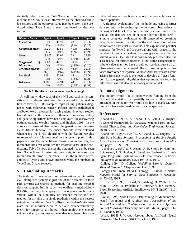
A well known drawback of the k-NN approach is its sen-sitivity to irrelevant attributes, the data used in the evalua-tion consists of 188 examples representing patients diag-nosed with colorectal cancer. Fifteen clinico-pathologicalattributes were recorded for each patient. Previous studieshave shown that the relevance of these attributes vary widelyand genetic algorithms have been employed for discoveringoptimal attribute weights [Anand and Hughes, 1998]. In theabsence of censored observations the genetic algorithm usesas its fitness function, the mean absolute error obtainedwhen using the k-NN algorithm with the feature weightsrepresented by a “chromosome” in the genetic pool. In thispaper we use the same fitness measure as minimising themean absolute error optimises the informativenss of the pre-dictions. Table 7 shows the results obtained. As can be seenfrom Table 6 and 7, using attribute weights decreases themean absolute error of the model. Also, the number of ex-amples of Type 1 and 4 have increased while the numbers inType 2 and 3 have reduced.

5 Concluding RemarksThe inability to handle censored observations within artifi-cial intelligence systems is just one of the obstacles in theirpath towards acceptance as methods for enabling medicaldecision support. In this paper, we outlined a methodology(Ck-NN) that may be employed to incorporate such obser-vations within the similarity or distance metric and themethod for arriving at a single prediction within the nearestneighbour paradigm. Ck-NN utilises the Kaplan-Meier esti-mate for the survivor curve to derive a distance/similaritymetric for categorical attributes. It then employs elements ofevidence theory to represent the evidence gathered, from the

retrieved nearest neighbours, about the probable survivaltime of patients.

A rigorous evaluation of the methodology using a largerdata set and by following up the censored observations inthe original data set, to record the true survival times is es-sential. The data set used in the paper does not lend itself toa more complete evaluation as all censored observationshave values greater than 60 months and uncensored obser-vations are all less that 60 months. This explains the peculiarstatistics for Type 2 and 3 observations with respect to thenumber of predicted values that are greater than the ob-served values. One issue that has already presented itself asa clear goal for further research is that some categorical at-tribute value may not have a defined survival curve as allobservations may be censored. How do we compute its dis-tance from other categorical values? Another research issuearising from this work is the need to develop a fitness func-tion for the genetic algorithm that optimises not only theinformativenss but also the accuracy of the model.

AcknowledgmentsThe authors would like to acknowledge funding from theNuffield Foundation that partially supported the researchpresented in the paper. We would also like to thank Dr. AnnSmith for her useful medical statistics perspective.

References[Anand et al., 1996] S. S. Anand, D. A. Bell, J. G. Hughes.A General Framework for Database Mining based on Evi-dential Theory, Data and Knowledge Engineering Journal,18:189 - 223, 1996.[Anand and Hughes, 1998] S. S. Anand, J. G. Hughes. Hy-brid Data Mining Systems, Proceedings of the 2nd PacificAsia Conference on Knowledge Discovery and Data Min-ing, pages 13--24, 1998[Anand et al., 1999] S. S. Anand, A. E. Smith, P. Hamilton,J. S. Anand, J. G. Hughes, P. Bartel. An Evaluation of Intel-ligent Prognostic Systems for Colorectal Cancer, ArtificialIntelligence in Medicine, 15(2):193--214, 1999.[Collett, 1994] D. Collett. Modelling Survival Data inMedical Research, Chapman and Hall, 1994.[Faraggi and Simon, 1995] D. Faraggi, R. Simon. A NeuralNetwork Model for Survival Data, Statistics in Medicine,14:73--82, 1995.[Kasif et al., 1998] S. Kasif, S. Salzberg, D. Waltz, J. Ra-chlin, D. Aha. A Probabilistic Framework for Memory-Based Reasoning, Artificial Intelligence 104(1-2):297—312,1998.[/DYUDþ@Nada /DYUDþ. Data Mining in Medicine: Se-lected Techniques and Applications, Proceedings of theSecond International Conference on the Practical Applica-tions of Knowledge Discovery and Data Mining, pages. 11--31, London, 1998.[Wyatt, 1995] J. Wyatt. Nervous about Artificial NeuralNetworks, The Lancet, 346:1175 - 1177, 1995.

Predicting Surgical Outcome in Temporal Lobe Epilepsy Patients Using a Naïve Bayes Classifier.

Antel SB, M.Sc.1,3, Li LM, MD 2,3, Cendes F, MD, PhD2,3, Olivier A, MD, PhD, FRCS(C)2, Andermann F, MD,FRCP(C)2, Dubeau F, MD, FRCP(C)2, Kearney RE, PhD1, Shinghal R, PhD4, Arnold DL, MD, FRCP(C) 2,3

Departments of Biomedical Engineering1, and Neurology and Neurosurgery2, McGill University.MR Spectroscopy Unit3, Montreal Neurological Institute and Hospital.

Department of Computer Science4, Concordia University.Montreal, Canada

Objective: To develop a machine learning-basedclassifier to predict surgical outcome in patients withtemporal lobe epilepsy (TLE).Method: We studied 81 patients with medicallyrefractory TLE who underwent surgical treatment. Inaddition to being clinically evaluated, patients werepre-surgically investigated with EEG, protonmagnetic resonance spectroscopic imaging (MRSI)and magnetic resonance volumetric (MRV) analysis.Outcome was measured using Engel’s classificationsystem, which we adjusted by combining Classes I &II (denoted as Group I) and Classes III & IV (denotedas Group II). A leave-one-out naïve Bayes classifierwas developed, using results from the aboveinvestigations as inputs.Results: The naïve Bayes classifier correctlypredicted the surgical outcomes of 49/54 (91%) ofGroup I patients, and 16/27 (59%) of Group II cases.The overall accuracy rate in predicting outcome was65/81 (80%)Conclusion: Reliable pre-surgical evaluation of apatient’s chances for a successful surgical outcome isfeasible using machine learning techniques.Predictive factors can be found among MRSI andMR volumetric data.

IntroductionSurgical treatment, via a selective

amygdalohippocampectomy (SAH) or an anterior temporallobe (ATL) resection, has been shown to be an effectivemeans of seizure control for about 70-80% of patients withmedically refractory temporal lobe epilepsy (TLE) [1].However, pre-surgical investigation of patients is costly,requiring weeks of hospitalization and monitoring via videoEEG and telemetry in highly specialized units. Even withsuch careful observation, approximately 20-30% of patientswill not obtain maximal benefit from surgery. In addition,any neurosurgical procedure carries a certain degree of risk.Therefore, given the risks and costs associated with thistype of treatment, a more efficient means of pre-operativeidentification of those TLE patients who stand to benefitfrom surgical intervention would be a valuable tool. Ouraim in this study was to develop a machine learning-basedclassifier to perform this task.

There are four criteria that such a classifier shouldfulfill to be of maximal clinical utility. First, it must be able

to make a prediction for an individual patient, rather thanmaking generalizations for a group of patients. Secondly,the classifier must use only pre-operative features as inputs.Thirdly, the classifier should be able to provide a measureof how confident it is in each prediction, i.e., posteriorprobabilities should be measurable. Lastly, the workings ofthe classifier must be transparent enough that aneurosurgeon or clinical epileptologist without abackground in artificial intelligence can understand the“reasoning” upon which a prediction is based, without in-depth knowledge of the underlying mathematics.

A number of studies have examined variousfactors as they relate to the prediction of surgical outcomein TLE patients. While these studies provide valuableinformation which can be used when designing a classifier,none fulfill all the above-stated criteria.

Many studies have investigated the relationshipbetween hippocampal atrophy and surgical outcome. Aconsensus finding is that unilateral hippocampal atrophy isa predictor of a good surgical outcome [2-5]. Bilateralhippocampal atrophy has been reported to reduce thechances for a good outcome [3]. Among patients withbilateral hippocampal atrophy, a recent study from our unithas shown that proton magnetic resonance spectroscopicimaging (MRSI) yields important information for theprediction of surgical outcome. Specifically, a low ratio ofN-acetylaspartate (NAA, a marker of neuronal integrity) tocreatine (Cr) in the contralateral posterior temporal lobesuggests diminished chances for a good outcome [6].However, because these studies examine only groupdifferences, they do not make predictions of an individual’schances for a successful surgical outcome.

Several studies have been able to generateindividual predictions for surgical outcomes. One studyreported success at discriminating between a group ofcompletely seizure free TLE patients and a group of TLEpatients who were nearly seizure free following surgeryusing artificial neural networks [7]. However, it may bedifficult for physicians to understand how a neural networkproduces its predictions, which diminishes its utility in aclinical context.

A recent study [8] reported encouraging success atdeveloping a predictive model, using logistic regression, todiscriminate between epilepsy (both TLE and extra-TLE)patients with an excellent chance of being seizure-free post-surgically and those with less than a 50% chance of the

same. However, post-surgical pathological analysis ofexcised tissue is used to obtain a feature in their model, andthus, while their classifier is a promising prognostic tool, itcannot be used to assist in pre-surgical evaluation ofpatients.

We have developed a naïve Bayes classifier topredict surgical outcomes of TLE patients, and which meetsthe conditions set out above. The classifier is basedprimarily on pre-operative magnetic resonance volumetry(MRV), which allows quantitative measurement of brainstructures, and proton magnetic resonance spectroscopicimaging (MRSI), which permits in vivo measurement ofbrain metabolites. Both modalities are non-invasive andrequire approximately an hour to perform. The classifier isconceptually simple, can produce a prediction for eachindividual patient, and can attach a posterior probability toeach prediction.

MethodsPatients

Our patient database consisted of 81 patientsdiagnosed with TLE (mean age 35 +/- 11.2 years). Thedatabase consisted of 31 males and 50 females. All patientsunderwent surgical treatment for TLE; 41 patientsunderwent anterior temporal lobe (ATL) resection, and 40patients underwent a selective amygdalohippocampectomy(SAH). No significant differences were found betweenthese two patient groups on any of the variables availablefor this study. Surgical outcomes were assessed usingEngel’s modified classification scheme [18]. Thebreakdown of the patients’ surgical outcomes was asfollows: 53 patients with Class I outcome (free of seizuresor residual auras), 1 with Class II outcome (less than 3seizures per year), 12 with Class III outcome (worthwhileimprovement), and 15 with Class IV outcome (noworthwhile improvement). We consolidated the patientsinto two groups (denoted as Group I and Group II) to obtainlarger and somewhat less disparate class sizes. Group I(n=54) consisted of patients who were seizure-free or nearlyseizure-free following surgery (Engel’s Class I & II).Group II (n=27) consisted of the remaining patients(Engel’s Class III & IV).

MR InvestigationsMR imaging was performed on a 1.5T scanner

(Philips Medical Systems, Best, The Netherlands). Sagittaland coronal T1 weighted images were acquired (TR=550ms, TE=19 ms), followed by axial proton density(TR=2000 ms, TE=20 ms) and T2 weighted (TR=2100 ms,TE=20, 78 ms). In order to perform volumetric studies ofthe hippocampi and amygdalae, T1 weighted, 1 mm thick,contiguous slice gradient-echo volume acquisition of thewhole brain was acquired. Quantification of volumes wasperformed using previously published methods [9].

MRSI of the temporal lobes was performed on thesame scanner, in a separate session. Following acquisition

of scout images in the axial and sagittal planes, a multi-slicetransverse spin-echo MRI (TR=2000 ms, TE=30 ms) wasobtained. The volume of interest (VOI) incorporated partof the head of the hippocampus, as well as the entire bodyand tail of the same. Also included in the VOI wereportions of gray and white matter in the mid and posteriortemporal lobe. The dimensions of the VOI were 85-100mm on the left-right axis, 75-95 mm on the anterior-posterior axis, and 20 mm in thickness.

A water suppressed MRSI was acquired from theVOI (TR=2000 ms, TE=272 ms, 250x250 mm FOV, 32x32phase-encoding steps), followed by a MRSI without watersuppression (TR=850 ms, TE=272 ms, 250x250 mm FOV,16x16 phase-encoding steps). Post-processing includedzero-filling the water unsuppressed MRSI to obtain 32x32profiles, followed by the application of a mild Gaussian k-space filter and an inverse 2D Fourier transformation toboth the water suppressed and unsuppressed MRSI. Theresulting time domain signal was left-shifted and subtractedfrom itself to improve water suppression [10]. Baseline-correction and measurement of resonance peak areas wereperformed on the individual spectra using locally developedsoftware.

Fifty-two healthy controls were examined withMR volumetry (1 mm slices: 30 patients, 3 mm slices: 22patients); MRSI was performed on 51 healthy subjects.MRSI and volumetric data were expressed as Z-scores,which describe the number of standard deviations above or

below the mean value of the normal controls.

EEG InvestigationAll patients underwent prolonged video-EEG

monitoring, using the International 10-20 system includingsphenoidal electrodes. EEG data were represented as alabel indicating predominant hemisphere(s) of seizureorigin: Left or Right (greater than 90% of seizuresoriginating from one side), Left>Right or Right>Left(greater than 70% of seizures originating from one side), orBilateral (less than 70% of seizures originating from oneside). Although EEG data were not used as inputs to theclassifier, designation of the various brain structures asipsilateral or contralateral was made in reference to theEEG results.

Design of naïve Bayes classifierA naïve Bayes classifier [11,17] is a machine

learning technique that assigns an instance consisting of anumber of attributes a1, a2,...an to the most likely class vnb ∈V , where V is the set of possible outcomes:

),...,,|(maxarg 21 nj

Vv

nb aaavPvj∈

= (1)

Using Bayes’ theorem, equation (1) can be expressed as

),...,,(

)()|,...,,(maxarg

21

21

n

jn

Vv

nbaaaP

vPvaaaPv

j

j∈= (2)

where P(vj) represents the prior probability of a randomlyselected training example having outcome vj. SinceP(a1,a2,…,an) is a constant independent of outcome group,equation (2) simplifies to

)()|,...,,(maxarg 21 jjn

Vv

nb vPvaaaPvj∈

= (3)

Class-conditional independence amongst the attributes isassumed, so that equation (3) can be simplified to

∏∈

=i

jij

Vv

nb vaPvPvj

)|()(maxarg (4)

We calculated P(ai|vj) using the Bayesian approach [11]:

mn

mpnvaP

cji

++=)|( (5)

where nc=is the number of training examples with aparticular value of ai and outcome vj; n is the total numberof training examples with outcome vj; p is the prior estimateof P(ai|vj); and m is the equivalent sample size. Since allvariables fed into the classifier were transformed intobinary variables, we set p=½. We chose an equivalentsample size of 2, as we used two outcome groups. Posteriorprobability for each prediction (i.e., a measure of howconfident the classifier was of the individual prediction) canbe calculated as

∑ ∏∏

=

j i

jij

i

nbinb

vaPvP

vaPvP

)]|()([

)|()(

yprobabilit

posterior(6)

Due to the limited number of patients, we elected touse the leave-one-out technique, whereby each of Ninstances is classified using the other N-1 instances as thetraining set. This technique provides an almost unbiasedestimate of the true accuracy of the classifier, serving as across-validation of our model [12]. The classifier wasimplemented in MATLAB 4.2 (The MathWorks Inc.,Natick, MA) running on a Red Hat Linux 5.2 platform.

An initial set of attributes was selected for inclusionin the classifier, based on whether a significant differenceexisted for an attribute across the two outcome groups.Other features were added based on findings in theliterature, such as the presence bilateral hippocampalatrophy. Clinical factors such as age and gender wereinitially included for completeness. Attributes were thenadded or deleted as needed to increase the accuracy of theclassifier. Table 1 summarizes the attributes ultimatelyused in the classifier. Within the table, v1 and v2 refer toGroups I and II, respectively.

Table 1. Inputs to the naïve Bayes classifier and theirestimated probabilities.Attribute P(ai|v1) P(ai|v2)Sex=Female 0.679 0.500Unilateral hippocampal atrophy 0.696 0.536Non-lateralizing bilateralhippocampal atrophy

0.018 0.107

No amygdaloid atrophy &R-score < -0.03 0.161 0.500Low NAA/Cr in contralateralposterior temporal lobe &contralateral Hc atrophy.

0.071 0.286

Hippocampal atrophy, amygdaloid atrophy, and lowNAA/Cr were defined on the basis of a Z-score less than–2. The R-score referred to in the table is defined asNAA/Cr Z score for the contralateral posterior temporallobe divided by age, a measure which we empirically foundto be useful for distinguishing between groups I and II.

It should be noted that some of the parameters inTable 1 do not meet the theoretical requirement of mutualindependence. However, it has been shown that a naïveBayes classifier can, in practice, achieve optimal resultseven if this assumption is violated [13].

ResultsThe naïve Bayes classifier developed in this study

correctly identified 49/54 (91%) of Group I patients, and16/27 (59%) of Group II cases. The overall accuracy rate inpredicting outcome was 65/81 (80%). Specificity (thenumber of cases correctly predicted to be in a group dividedby the total number of cases predicted to be in that group)was 82% (49/60) for Group I patients and 76% (16/21) forGroup II patients, respectively. Figure 1 displays theaccuracy and specificity for Groups I and II. Univariateanalysis revealed that NAA/Cr in the contralateral posteriortemporal lobe was significantly lower (p<.001) in Group IIpatients compared to Group I patients.

91%82%

59%

76%

0%

20%

40%

60%

80%

100%

Accuracy Specificity

Per

cent

age

Group I

Group II

Figure 1. Accuracy and specificity of classifier.

DiscussionThe naïve Bayes classifier developed in this study

provides a simple method of predicting surgical outcome inTLE patients. A key advantage of our classifier is theability to identify patients who will not be free or nearlyfree of disabling seizures following surgery. Over one-thirdof the patients identified as surgical candidates viaconventional means (i.e., consensus interpretation by expertepileptologists and neurosurgeons of EEG, neurological,neuropsychological, and neuroradiological investigations)did not experience a complete or near-complete eliminationof seizures post-surgically; our classifier identified almosttwo-thirds of these patients.

However, it is problematic to use the decision ofwhether to operate (made via conventional means asdescribed above) as a comparison for our classifier. Adecision to operate does not necessarily imply anexpectation of a seizure-free or nearly seizure-free outcome.The situation does arise whereby a patient will be operatedupon in the full knowledge that a Class III or Class IVoutcome is all that can be hoped for, based on the logic thata small improvement may be worth the risk to a particularpatient. Furthermore, patients deemed unsuitablecandidates for surgery did not undergo an operation, andtherefore it cannot be determined if the decision not tooperate (indicative of an expectation of poor surgicaloutcome) was correct.

Straightforward interpretation was one of thecriteria for a clinically useful classifier set out earlier. Theconditional probabilities for each attribute given eachoutcome class used in the naïve Bayes classifier in essenceconstitute a frequency table that can provide insight as tohow the predictions are made, even without knowledge ofthe algorithm behind the classifier. The majority of theattributes (3 out of 5) included in the classifier tested for theabsence of lateralizing abnormalities; either because theattribute was bilaterally abnormal, or because the attributewas bilaterally normal. Bilateral involvement suggestswidespread abnormalities, rather than a focal abnormalitythan can be easily excised via surgery. Lack of anabnormality suggests an inability to localize the point(s) ofseizure origin, complicating the effective resection of theseizure focus.

Previous studies report on the relationship betweennon-lateralizing hippocampal atrophy and poor surgicaloutcome [3,14]. We found analogous results in thespectroscopic data. NAA/Cr Z-scores in the contralateralposterior temporal lobe were significantly lowered in GroupII patients. This is reflected in two of the features used inthe classifier: R-score (NAA/Cr Z-score in the contralateralposterior temporal lobe divided by age) and thecombination of a low NAA/Cr Z-score in the contralateralposterior temporal lobe and contralateral hippocampalatrophy.

The only lateralizing feature used in the classifierwas the presence of unilateral hippocampal atrophy, which

has been widely reported as correlating with a positivesurgical outcome [2-5]. An apparently novel finding is thatgender is a predictive factor.

Perhaps the most important aspect of the classifierdeveloped in this study is that it does not directly rely onsurface or intracranial EEG recordings to make itspredictions. Methods of lateralizing seizure focus in TLEpatients have been developed [9] that approach the efficacyof EEG monitoring, using only MRSI and MRV data.Thus, a classifier independent of EEG results couldeventually lead to an integrated system of lateralization andprognostication, based only on MR data, that would reducetime and hospitalization expenses, and eliminate the risksassociated with the implantation of depth electrodes. Itshould be noted, however, that the contralateral andipsilateral designations in this and other studies are definedrelative to EEG findings, as EEG is the current gold-standard in clinical epileptology. Therefore, a classifiersuch as the one developed in this study will only be trulyEEG-independent upon the emergence of the combined MRinvestigations as the gold-standard for the evaluation ofTLE.

Further refinements include expanding theclassifier to classify patients into one of the four outcomeclasses in Engel’s scheme, rather than the two consolidatedgroups we used. A larger database of patients than iscurrently available may help facilitate this by providingsufficient sample size for each of the four outcome classes.A larger database would also allow us to detect more subtledifferences between the groups, perhaps increasing theaccuracy of the classifier.

It is premature to state that a classifier such as ourscan make the ultimate decision to operate on a particularpatient. Reduction in seizure frequency is only one aspectof surgical outcome; post-surgical cognitive function of thepatient is also an important consideration when decidingwhether to operate. The expansion of the classifier toinclude neuropsychological data to help predict such ameasure is therefore an important future objective.Furthermore, an outcome other than complete or near-complete elimination of seizures may in fact be aworthwhile improvement for a percentage of TLE patientswith particularly frequent seizures. The individualcircumstances of patients will still need to be consideredwhen evaluating the surgical option. Nevertheless, theresults of this study suggest that our classifier may provideassistance in identifying surgical candidates.

References

1. Engel J. Update on surgical treatment of the epilepsies.Neurology 1993; 43(8); 1612-1617.

2. Radhakrishnan K, So EL, Silbert PL, Jack CR, CascinoGD, Sharbrough FW, O’Brien PC. Predictors of outcome of

anterior temporal lobectomy for intractable epilepsy.Neurology 1998;51:465-471.

3. Arruda F, Cendes F, Andermann F, Dubeau F, VillemureJG, Jones-Gotman M, Poulin N, Arnold DL, Olivier A..Mesial atrophy and outcome afteramygdalohippocampectomy or temporal lobe removal. AnnNeurol 1996;40:446-450.

4. Knowlton RC, Laxer KD, Ende G, Hawkins RA, WongSTC, Matson GB, Rowley HA, Fein G, Weiner MW.Presurgical multimodality neuroimaging inelectoencephalographic lateralized temporal lobe epilepsy.Ann Neurol 1997;42:829-837.

5. Cascino GD, Trenerry MR, Sharbrough FW, So EL,Marsh WR, Strelow DC. Depth electrode studies intemporal lobe epilepsy: relation to quantitative magneticresonance imaging and operative outcome. Epilepsia1995;36(3):230-235.

6. Li LM, Cendes F, Antel S, Serles W, Andermann F,Dubeau F, Olivier A, Arnold DL. Prognostic features insurgical outcome of patients with bilateral hippocampalatrophy and intractable temporal lobe epilepsy (Abstr.).Neurology 1999; 52 (Suppl. 2): 161-162.

7. Grigsby J, Kramer RE, Schneiders JL, Gates JR, SmithWB. Predicting outcome of anterior temporal lobectomyusing simulated neural networks. Epilepsia 1998; 39(1):61-66.

8. Berg AT, Walczak T, Hirsch LJ, Spencer SS.Multivariable prediction of seizure outcome one year afterresective epilepsy surgery: development of a model withindependent validation. Epilepsy Research 1998; 29(3):185-194.

9. Cendes F, Caramanos Z, Andermann F, Dubeau F,Arnold DL. Proton magnetic resonance spectroscopicimaging and magnetic resonance imagin volumetry in thelateralization of temporal lobe epilepsy: a series of 100patients. Ann Neurol 1997;42:737-746.

10. Roth K, Kimber BJ, Feeney J. Data shift accumulationand alternate delay accumulation techniques forovercoming the dynamic range problem. J Magn Res 1980;41;302-309.

11. Mitchell TM. Machine Learning. Boston:WCB/McGraw Hill, 1997.

12. Hand DJ. Discrimination and Classification.Chichester: Wiley, 1981.

13. Domingos P, Pazzani M. Beyond independence:conditions for the optimality of the simple Bayesianclassifier. Proc 13th Int’l Conf Machine Learning1996;105-112.

14. Jack CR, Sharbrough FW, Cascino GD, Hirschorn KA,O’Brien PC, Marsh WR. Magnetic resonance image-basedhippocampal volumetry: correlation with outcome aftertemporal lobectomy. Ann Neurol 1992; 31:138-146.

15. Bloom D, Jasper H, Rasmussen T. Surgical therapy inpatients with temporal lobe seizures and bilateral EEGabnormality. Epilepsia 1960; 1; 351-365.

16. So N, Olivier A, Andermann F, Gloor P, Quesney LF.Results of surgical treatment in patients with bitemporalepileptiform abnormalities. Ann Neurol 1989; 25(5); 432-439.

17. Duda RO, Hart, PE. Pattern Classification and SceneAnalysis. New York: John Wiley & Sons, 1973.

18. Engel J, Van Ness PC, Rasmussen TB, Ojemann LM.Outcome with respect to epileptic seizures. In: Engel J, ed.Surgical treatment of the epilepsies. 2nd ed. New York:Raven Press, 1993:609-621.

Identification of patients at high cardiovascular risk : a critical appraisal ofapplicability of statistical risk prediction models.

Hervé Dréau Isabelle Colombet Patrice Degoulet Gilles Chatellier

Medical Informatics Department Broussais Hospital

96 rue Didot, 75014 Paris. France

AbstractAssessment of cardiovascular risk is widely proposed as abasis for taking management decisions among patientspresenting with hypertension or hypercholesterolemia. Ouraim was to critically assess use of risk equations derivedfrom epidemiological studies in the purpose of identifyinghigh risk patients.Risk equations were retrieved in the MEDLINE databaseand then applied to a data set of 118 patients. This data setwas an evaluation study of the clinical value of WorldHealth Organization 1993 hypertension guidelines for thedecision to treat mild hypertensive patients We calculatedagreement: 1) between equations and 2) between equationsand the decision to treat taken by the physician.Most models were not applicable to our population, mainlybecause the original population had a narrow age range orcomprised only males. Between-model agreement wasbetter for the lower and upper risk quintiles than for the 3other risk quintiles (0.58, 0.33, 0.34, 0.45, 0.70, from thelower to the upper risk quintile). When using an arbitrarythreshold for defining high risk patients(i.e. >2% per year),we observed a huge variation of the proportion of patientsclassified at high risk (from 0 to 17%). There was a pooragreement between risk models and the decision to treattaken by the physician.These results suggest that risk-based guidelines should bevalidated before their diffusion.

1. Background

All guidelines related to the cardiovascular field(hypertension, diabetes or lipid management) presentlypropose to manage patients using an explicit reference to theabsolute cardiovascular risk1. Many epidemiological studieshave provided various risk prediction statistical models inthe cardiovascular domain. The characteristics of thesestudies vary widely in terms of design, origin of the studypopulation, inclusion criteria, measured outcome criteriaand period of follow-up. Moreover, the models also differboth in the type of underlying statistical method and in thepredictive variables they used.

Therefore, using these models to predict the cardiovascularrisk of a given individual, could be questionable. Beforechoosing a given model, it is mandatory to comparecharacteristics of the actual population to which theconsidered individual belongs to those of the originalpopulation, to define the internal validity of the model(quality of the study, range of the predictor variables…) andto obtain data on external validity (test of the model inanother population). Among the cardiovascular risk models, those obtained fromthe Framingham study have been validated in variouspopulations, in the United States, in Australia and inEurope. However, in Europe, and particularly in France,where prevalence of coronary heart disease (CHD) is low2,several other models are available. Laurier et al addressedthe problem of absolute predictive performance andcorrected the original Framingham model by calibrating it to

the French population3. Other models from Germany,Australia, and Scotland could also be used. Ideally, it wouldbe necessary to assess the predictive performance of eachmodel against the real risk. As a first step toward validation,the present work compare how the risk estimated bydifferent models could be predictive of a medical decisiontaken in hypertensive patients by a physician following acurrent validated international practice guideline.

2. Objective

To evaluate the usability and the agreement ofcardiovascular risk prediction models derived from severallarge epidemiological studies, in the context of the decisionto treat mild hypertension. We first examined the discriminative performance of themodels by looking at the ability of models to classifypatients according to levels of risk. Then, performance ofeach model was assessed by reference to the physiciandecision to treat or not to treat patients with antihypertensivedrugs.

3. Methods

3.1 Data set

We used data from a previously published clinical study 4.Briefly, non-obese patients referred at the BroussaisHospital hypertension clinic with untreated suspected orknown essential uncomplicated mild hypertension, aged 21years or more were included in a protocol designed foridentifying those patients needing treatment. At inclusion,the 118 included patients who had usual laboratory andother diagnostic tests and were then followed up eachmonth, for 6 months. Need for treatment was determined bya physician following the World Health Organization 1993guidelines for the treatment of mild to moderatehypertension : briefly, drug treatment could be instituted onthe basis of both diastolic or systolic blood pressure (BP)level over repeated visits and the physician's estimate ofcardiovascular risk according to known risk factors for CHDand stroke. Physician's decision was considered as the goldstandard in the present work.

3.2 Models: analysis of the literature Models of cardiovascular risk were retrieved through aMEDLINE search. A model was selected if 1) it was basedon a prospective cohort study; 2) it provided an estimate ofabsolute risk. A model was defined as calculable when itprovided all the parameters necessary to calculation, and asusable when all necessary variables were available in ourdata set. Finally, usable models were applied to the 118 patients ofour data set, using the data of original papers for definingapplicability of each model. Thus, minimum and maximumvalues of each quantitative variables were used asapplicability criteria of a given model for a given patient.For example, a model developed on a sample having adiastolic BP between 90 and 120 mm Hg was applied onlyto patients having a diastolic BP within this range. 3.3 Statistical methods To assess agreement between the different models, we useda 2-class Kappa coefficient for unbalanced observationsbased on a tertile classification of absolute risk estimated byeach model. High-risk patients were those belonging to theupper tertile, and low-risk patients those in the 2 othertertiles 5. For models using the same subset of our data set,we used a 5-class Kappa coefficient based on a quintileclassification of absolute risk estimated by each model. Area under the Receiver Operating Characteristics curve(ROC) was used to assess and compare risk classificationsderived from the various models to our gold standard, thedecision to treat taken by the physician.

The R statistical software (Ross I, Gentleman R. R: ALanguage for Data Analysis and Graphics Journal ofComputational and Graphical Statistics 1996;5:299-314)was used for calculations.

4. Results

1.1 4.1 Description of modelsAccording to our inclusion criteria, 27 calculable modelsfrom 8 epidemiological studies were identified.Epidemiological characteristics of these models aresummarized in Table 1. Three different statistical modelswere used : Cox regression model (n=4), multiple logisticregression model (n=11) and Weibull time failureaccelerated regression model (n=12).Among the 27 calculable models, 26 were usable. TheLaurier equation was not obtained through anepidemiological study, but represents the calibration of aCHD Framingham equation to the French population.The selected models comprised 4 to 13 different predictors(variables or combination of variables) among which onlyage was common to all models (BP and tobaccoconsumption are in all models but with different coding).For a given variable, definition and measurement were notthe same across the studies: differences concerned BP(number of measurements), tobacco consumption(quantitative or qualitative variable), left ventricularhypertrophy.The outcome variable could be either a specific disease (i.e.myocardial infarction), or a composite end-point (i.e. CHD).Definition of outcomes also varied across studies. Forexample, even in models coming from the sameepidemiological study, Framingham, CHD could bedescribed differently (i.e. comprising or not anginapectoris).4.2 Application to data setThe Framingham and Laurier models could not be used in 4of our patients (all are aged less than 30 years). With thePROCAM model, only 45 patients remained eligible forcalculation (49 were excluded because they were women,and 23 men were excluded because they were outside theage range ). The Busselton models could not be used in 24of our patients (all because of an age < 40 years). TheCCHS model could be applied in only 28 patients (all theother were excluded because they were under 55 years). TheFrench Paris Prospective Study (PPS) model could beapplied only to 26 patients (all women and 43 men outsidethe age range were excluded). The Dundee and ERICAmodels could be applied in 41 (all women and 28 men wereexcluded). For 4 patients there were no applicable models.AgreementUsing the 2-class kappa coefficient, the agreement beyondchance between the 26 usable models applied to 114 /118

patients of our data set was 0.68, a value corresponding to agood agreement.Using the kappa coefficient after classification intoquintiles, the Framingham (n=18), and Laurier modelsapplied to 114 patients. They had a global agreementbeyond chance of 0.48. Agreement was better for the lowerand upper risk quintiles (0.58, 0.33, 0.34, 0.45, 0.70, fromthe lower to the upper quintile).Validation against the gold standardIn our data set, 48 of the 118 patients (40.1%; 95% CI:31.9% - 50.1%) have been treated with antihypertensivedrugs at the end of the follow-up. These patients correspondto high risk patients defined by a physician applying apractice guideline. Area under the ROC curve of the variousmodels against the physician's decision (gold standard)ranged from 0.44 to 0.78 for the different models (table 2).When using an absolute cut-point for defining high-riskpatients needing a pharmacological treatment, for examplethe widely used. 2 % annual risk proposed in the guidelinesof the European Society of Cardiology, there is a hugevariation in the proportion of patients classified at high risk,depending on both the study setting, and the outcome used(table 2). The proportion of patients classified at high riskand their confidence intervals for selected studies were asfollows:• Framingham (CHD), 11 / 114 patients (9.7%;

95% CI: 4.2% - 15.1%)• Framingham (CVD), 17 / 114 patients (14.9%;

95% CI: 8.4% - 21.4%)• Laurier (CHD), 6 / 114 patients (5.3%; 95%

CI: 1.2% - 9.4%)• Procam (MI) , 3 / 45 patients (6.7%; 95%

CI: 1.7% - 19.3%)• Busselton (CHD death), 1 / 94 patients (1.1%; 95%

CI: 0.06 % - 6.6%)• PPS (CHD), 0 / 26 patients (0% ; 95%

CI: 0.35% - 16.2%

Table 2 also provides the proportion of patients having arisk below 2% per year and 0.5% per year (a very low risklevel for which only non pharmacological treatment wouldbe advised). Both proportions varied widely according tostudies. However, whatever the model chosen, a highproportion of patients at low risk or even at very low riskwere treated with drugs by the physician.

1. Discussion

Many diseases are now preventable if adequate screeningand treatment are performed. For example, systematicscreening is proposed for colon and breast cancer after 50years, and at any age for cardiovascular disease. However,to avoid screening in low risk patients, it would beinteresting to target interventions or screening towards high

risk patients. In this respect, using statistical models basedon large prospective studies seems to be the best solution.In the cardiovascular field an important number of potentialpredictive risk models usable in prevention are available,and the present review is probably not complete. A moreexhaustive selection and comparison of logistic risk modelscan be found in Chambless and al 6. When trying to find a model, the first obstacle is the lack ofinformation on some parameters of the model in the originalpaper: often only relative risk for the different risk factorsare given. Second, variables found in some models may notbe available in the user data set, either for coding reasons(tobacco consumption rather than number of cigarettes perday), or missing variable in the database. Even if thevariable is present, definition may differ since there is noagreement on the way of measuring a given factor: forexample, how many measurements define the bloodpressure? Third, inclusion criteria and range of variableslimit applicability to population having comparablecharacteristics. Thus, even when using the most applicablemodel (Framingham study) it was not possible to calculatean absolute risk for all the people referred in anhypertension clinic. The relatively low agreement betweenmodels result probably from a mixture of measurement,statistical and epidemiological differences. The practical use of equation is made difficult by the choiceof equation and the choice of a risk threshold. The samepatient could be classified at high or low risk just because adifferent equation has been used for calculating risk (Table2). This is a major problem. In the meanwhile, it seemstherefore advisable to favor the use of the Framinghamequation, because it is more applicable than the other ones,and has been widely validated outside the United States.The level of absolute risk beyond which define a high riskpatient (i.e a patient needing treatment) is purely arbitrary.For example, European and New Zealand guidelines use a 2% annual risk, whereas the UK guidelines propose a 3%annual absolute risk. At a first glance, it seems questionable to use the decision totreat taken by a physician as the gold standard to comparethe performance of the risk models. However, this choiceenlightens the discrepancy between a decision based onmultifactorial absolute risk models and practice even if thephysician's decision is based on well established guidelines.There are several explanations to the great percentage of ourpopulation who has been treated in spite of a low absoluterisk. First, our population is younger (mean age: 51 years)than the Framingham one (mean age: 65 years) and it is wellknown that the use of absolute risk tends to favorintervention for aged patient because age is an importantand not modifiable risk factor of cardiovascular diseases,taken into account in all the models, for example there is nopatient at high risk of CHD predicted by the Framinghammodel in the younger half of our population. A solution to

this problem could be to use the marginal absolute risk (riskof the patient minus the risk of a person of the same genderand age without risk factors) to classify people at high levelof risk. However, there is no definition of a "high" marginalrisk! Second, a 10-year prediction is too short, and thephysician may subjectively use a more long term riskestimate. In conclusion, we show that there are many limitations to theuse of prediction models. Individualized life time predictionwill undoubtedly improve identification of high risk patients7. However, only a randomized controlled trial comparing arisk-based strategy to the traditional strategy will be able todetermine if risk prediction improves the quality of care.

2. References

A complete list of references on models is available fromrequest to the authors.DeLong, E.R., DeLong, D.M. & Clarke-Pearson, D.LComparing the areas under two or more correlated receiveroperating characteristic curves: A nonparametric approach..Biometrics 1988;44:837-845.

1. Recommendations of a Task Force of the European Societyof Cardiology and the European Resuscitation Council onThe Pre-hospital Management of Acute Heart Attacks.Resuscitation 1998;38(2):73-98.

2. Renaud S, de Lorgeril M. Wine, alcohol, platelets, and theFrench paradox for coronary heart disease. Lancet1992;339(8808):1523-6.

3. Laurier D, Nguyen PC, Cazelles B, Segond P. Estimationof CHD risk in a French working population using amodified Framingham model. The PCV-METRA Group. JClin Epidemiol 1994;47(12):1353-64.

4. Chatellier G, Abergel E, Battaglia C, Menard J. Do WHO-ISH guidelines identify high risk mild hypertensivepatients?. Arch Mal Cœur Vaiss 1998;91(8):967-70.

5. Fleiss JL Statistical methods for rates and proportions,2nd

ed. J Wiley. p223-224, 1981.6. Chambless LE, Dobson AJ, Patterson CC, Raines B. On the

use of a logistic risk score in predicting risk of coronaryheart disease. Stat Med 1990;9(4):385-96.

7. Lloyd-Jones DM, Larson MG, Beiser A, Levy D. Lifetimerisk of developing coronary heart disease . Lancet1999;353(9147):89-92.

Table 1: Main characteristics of the calculable cardiovascular risk prediction models.Study n° of

modelsCountry Study

Beginningage (sex#) Statistical

model¶Variables Outcome Usability

Framingham 12 US 1948 30-74 (1) W (a) Multiples‡ at 4-10years

114/118

Framingham 1 US 1948 30-74 (1) L (b) CHD at 10 years 114/118Framingham 1 US 1948 30-74 (1) C (e) Stroke at 1-10 years 114/118Framingham 1 US 1948 30-74 (1) L (f) Intermittent

claudication at 4 years114/118

Framingham 1 US 1948 30-74 (1) L CHD at 8 years 114/118Framingham 2 US 1948 30-74 (1) L (a) CHD death at 10 years 114/118Laurier 1 Fr - 30-74 (1) C (a) CHD at 4-10 years 114/118Busselton 1 Au 1966 40-74 (1) L (c) CHD death at 10 years 94/118Busselton 1 Au 1966 40-74 (1) L (c) + BMI CHD death at 10 years 94/118Procam 1 De 1979 40-65 (2) L (d) MI at 8 years 45/118Dundee 1 Scot 1984 40-59 (2) L (h) CHD at 5 years 41/118PPS 1 Fr 1967 43-54 (2) C (g) CHD at 5 years 26/118Copenhagen 1 DA 1976 55-84 (1) C (e) Stroke at 10 years 28/118ERICA 1 Europe 1982 40-59 (2) L (i) CHD death at 6 years 41/118WCGS 1 US 1960 39-59 (2) L CHD at 8.5 years 0/118¶: W: Weibull, C: Cox Model, L: Logistic Model.‡: CHD, cardiovascular disease (CVD), myocardial infarction (MI), Stroke, CHD death, CVD death prediction for a 4 to 10years interval, using either systolic BP or diastolic BP.#: 1 both, 2 men only(a) systolic BP or Diastolic BP, age, gender, smoking status (Y/N), diabetes (Y/N), left ventricular hypertrophy (Y/N), totalcholesterol (TC) , HDL cholesterol (HDL-C) with interaction between variable.(b) five levels for TC, five levels for HDL-C, five levels for BP, diabetes, smoking status, age.(c) age, Systolic BP, TC, Smoking status.(d) systolic BP, age, TC, HDL-C, triglycerides, smoking status, familial history of myocardial infarction, angina pectoris.(e) age, Systolic BP, diabetes (Y/N), smoking status (Y/N), left ventricular hypertrophy (Y/N), atrial fibrillation, CVD, anti-hypertensive treatment.(f) four levels for both systolic and diastolic BP, gender, tobacco consumption (cig/d), diabetes (Y/N), age, TC.(g) TC, Systolic BP, tobacco consumption (cig/d), diabetes (Y/N), age.(h) systolic BP, tobacco consumption (cig/d), age, TC(i) systolic BP, tobacco consumption (Y/N), age, TC, body mass index (BMI).

Table 2: Influence of model and threshold of absolute risk (AR) on the decision to treat.Model n° of patients ¶

(treated/total)Outcome‡ Risk >

2% /yearsUntreatedand AR >2%/years

Treatedand AR <2% /years

Treated andAR <

0.5%/years

ROCcurve

Framingham (SBP) 48/114 CHD 11 5 42 24/56 0.58Framingham (DBP) 48/114 CHD 12 5 41 20/54 0.59Framingham (categorical) 48/114 CHD 10 5 43 14/38 0.56Laurier Model 48/114 CHD 6 1 43 28/75 0.58Framingham (SBP) 48/114 CVD 17 8 39 7/30 0.59Framingham (Cox model) 48/114 stroke 0 - - 37/94 0.59Framingham (SBP) 48/114 IC (4) 0 - - 45/111 0.60Framingham (SBP) 48/114 CHD (8) 9 4 43 24/37 0.60Busselton 45/94 CHD-death 2 0 43 39/77 0.51PROCAM 24/45 MI 3 2 23 18/31 0.44PPS 13/26 CHD (5) 0 - - 9/21 0.54CCHS 9/28 stroke 2 0 7 1/12 0.78Dundee 23/41 CHD (5) 2 0 21 6/10 0.49ERICA 23/41 CHD-death (6) 0 - - 21/39 0.52¶: Number of patients in whom the given equation was applicable.‡: CHD: coronary heart disease, CVD: cardiovascular disease, MI: Myocardial infarction, IC : intermittent claudication.

AbstractWe have compared different regression diagnostic meth-ods for detection of influential cases in a model that pre-dicts death from traumatic injuries. For the purposes ofthis work, we defined "influential" as an outlier whoseremoval might be beneficial to the prognostic model. Theregression diagnostic methods involved "unicase" and"multicase" determination of case influence on modelpredictive performance. Multicase determinations wereperformed using two methods: a sequential "backward"selection of cases and a non-sequential genetic algo-rithm.A case whose removal resulted in a model that had betterfit (measured by the area under the ROC curve, or AUC)was considered influential. The unicase and sequentialbackward selections resulted in a final model that hadexcellent fit (AUC=0.98 in training set), but that lostsignificant predictive capability (AUC=0.78 in test set).The genetic algorithm produced a final model that keptfewer cases, had good fit (AUC=0.95), and retained pre-dictive capability (AUC=0.86). These results indicatethat a genetic algorithm approach to case selection mayyield better results than a unicase or a sequential multi-case approach, possibly because of its ability to detectsets of cases that are influential en bloc, but may not besufficiently influential when considered in isolation.

1 IntroductionPrognostic models of trauma have been extensively in-vestigated using different regression and machine learn-ing algorithms and some are currently used in clinicalpractice [1-4]. Determining case influence is importantfor building and continuously updating these models asnew cases are added. Detecting and removing influentialcases that bias prognostic models are desirable in orderto evolve a training set of "good" cases. Case influencedetermination is developed under the name regressiondiagnostics, and involves the identification of not onlyundesirable outliers, but also cases that have a strongerimpact on the prognostic model's estimated parameters orfinal fit. These features are often highly interrelated.Considerable debate has centered on what constitutes agood method for influential case detection. Several indi-

ces have been proposed: (standardized and studentized)residuals, leverage, Cook’s statistic and its variants,etc.[5,6]. Graphical methods to help visualize influencehave also been proposed [7]. Other methods have beenproposed by machine learning researchers [8,9]. Mostinfluence detection methods are based on the effects ofcase deletion on the parameters of the model or on its fitand predictive ability. Because of computational intrac-tability, the methods are usually used in a “unicase”manner (i.e., just one case is deleted at a time). However,it has been noted that some cases may not be influentialwhen considered independently, but may become influ-ential when considered en bloc [5,6,7]. This influencemay be detected if deletion is used in a “multicase” man-ner (i.e., several cases are deleted at a time). Consider-ing all subsets of cases for influence detection is intrac-table (requiring 2m calculations for m cases). Therefore,certain heuristics need to be used in practice.In this work, we were interested in the detection and re-moval of undesirable outliers from a particular data setfor the construction of a prognostic model that general-ized well to a set of previously unseen cases. We haveimplemented unicase and multicase influence detectionmethods for logistic regression. Two multicase modelswere built: one based on backward selection and anotherbased on a genetic algorithm. We describe and comparethese different methods and illustrate them with a modelaimed at building a prognostic index from a data set ofacute trauma patients.

2 Material and Methods

2.1 DataWe used a dataset of 300 patients from a random selec-tion of patients admitted to the University of New Mex-ico Trauma Center between 1991 and 1994. The com-plete data set of 300 patients is described in [10] andavailable on the Internet at http://stat.unm.edu/~fletcher.The collection has been used previously in [11]. Eachcase in the data set had information on age, Injury Se-verity Score (ISS), Revised Trauma Score (RTS), Typeof Injuries (TI), and outcome (survival or death). Thevariable ISS has numeric values on a scoring scale, RTS

Influential Case Detection in Medical PrognosisLucila Ohno-Machado Staal VinterboDecision Systems Group

Brigham and Women's Hospital andHealth Sciences and Technology Division,

Harvard Medical School/MITBoston, U. S. A.

Knowledge Systems GroupDept. Computer and Information Sciences,

Norwegian Universityof Science and Technology

Trondheim, Norway

is continuous and TI is binary ("blunt" or "penetrating").We selected this data set because we knew from the lit-erature [10] that it could produce reasonable prognosticindices and because its size (in terms of variables andcases) was adequate for this experiment.For some experiments, the full data set was randomlysplit into a training (n = 152) and a test (n = 148) set,such that the same number of deaths appeared in eachdata set. The training set was used to build the modelsand select cases, and the test set was left out for evalua-tion purposes. In other experiments, we used the full dataset. Table 1 shows the means of each variable for thetraining, test, and full data sets.

ISS TI RTS age survival

Training 14.296 0.243 7.265 31.664 0.927

Test 14.263 0.256 7.309 31.148 0.925

All 14.280 0.25 7.286 31.41 0.926

Table 1. Variable means for training (n = 152), test (n = 148),and full data sets (n = 300).

2.2 MethodsWe built a logistic regression model using all cases andrefer to it as the “baseline” model. We built unicase andmulticase deletion methods using C and the SAS macrolanguage. All logistic regression models were built usingthe SAS procedure LOGISTIC [12] and the same defaultparameters. The area under the ROC curve (AUC) wasmeasured for all methods described below.

Unicase deletionWe constructed 152 different training sets in which onepatient was removed. The resulting AUC was recordedfor each model. The AUCs corresponding to the use ofthe models in the test set of 148 patients were also re-corded for evaluation purposes. Cases were consideredinfluential if the models in which they were removedresulted in high AUCs (as measured in the training set ofremaining 151 cases). The AUCs for all models weresorted in descending order. The "most influential" caseswere defined as those corresponding to models in the topof the sorted file. For example, the topmost individualcase is influential because its removal causes the AUC toincrease from 0.91 to 0.951.

Multicase deletion

Exhaustive evaluation of all 2152 subsets of cases is not fea-sible. Therefore, we used certain heuristics to constructsubsets that were based on sequential stepwise deletionand guided sampling using a genetic algorithm.

1 The bottom most individual could also have been considered "influ-ential" because its deletion causes the AUC to drop from 0.91 to0.90, but we have not included this case in our definition.

• Backward selectionWe used a heuristic borrowed directly from variable se-lection methods. We start with the full data set, and buildmodels in which each case is removed, as in the unicaseselection above. We then remove the case correspondingto the model with highest AUC and use the reduced dataset to determine the next case to be removed, using thesame criterion. This strategy has been suggested by Cookand Weisberg [6] and Belsey et al.[5], and requires thatwe construct the following number of models:

∏−=

−1

0)(

m

iin

where m represents the number of cases removed.• Genetic AlgorithmFor an introduction to genetic algorithms, see [13]. Weused a measure of fitness for a selection of cases that hasbeen used in another study for variable selection [14].Given a training set C, and a selection of cases v, weconstruct a logistic regression model lC(v). We evaluatethe model using the AUC, and represent this evaluationas a(lC(v)). For a total of n cases, and m cases in selec-tion v, we use the following fitness function:f(v,C) = a(lC(v)) + ρ∗ (n - m)/n.The second term rewards a parsimonious selection ofcases, and is weighted by parameter ρ. We used ρ = 0and ρ =.05 in this experiment. Population size was fixedat 50 (each “individual” in the population is a certainsubset of all cases), and cross-over, mutation, and inver-sion probabilities were set at 0.3, 0.05, and 0.1, respec-tively. The stop criterion was the lack of improvement ofthe average fitness of the population after 10 generations.

3 ResultsWe used the test set in order to assess how generalizablethe results would be in a previously unknown set ofcases. Table 1 shows that the data split we used pre-served the main characteristics of the data set. Since wenoted significant differences between the performance onthe training and test sets after performing case deletion,we also tested the different case selection methods usingthe full data set, so that we could identify whether certaincases deemed influential were just artifacts of our par-ticular data split.

3.1 Baseline Regression DiagnosticsData split (152 training, 148 test)All cases in the training set were included in this model.The AUC was 0.91 in the training set and 0.88 in the testset. By using the option INFLUENCE inSAS/LOGISTIC [12], we obtained the following 5 mostinfluential2 cases (in descending order), using the statis-tics below:

2 Note that this definition of an influential case does not assume thata case is necessarily a "bad case", as we have defined in this work.

• Pearson residual: 34,120,136,6,24.• Deviance Residual: 34,120,136,6,90.• Hat Matrix Diagonal: 4,3,31,46,90.• C: 4,3,24,120,90.• CBAR: 4,3,24,120,136.• Change in Deviance to Deletion: 34,120,136,4,24.• Change in Pearson χ2 statistic due to deletion:34,136,120,24,6.

Full data setAll 300 cases in the training set were included in thismodel. The AUC was 0.90. Cases from what was the testset in the previous experiment were numbered 153 andhigher. The bolded numbers refer to influential cases thatcoincided with those of the training set:• Pearson residual:34,191,219,136,180,24,6,238,273,249,90.

• Deviance Residual:34,191,219,136,180,6,24,238,90,273,249.

• Hat Matrix Diagonal:4,83,3,129,296,96,139,32,170,211,154,90.

• C: 120,90,24,139,273,249,191,34,219,238,228,11.• CBAR:120,24,90,139,191,273,249,34,219,238,228,117.

• Change in Deviance to Deletion:34,191,120,219,136,24,238,90,273,249,11,228.

• Change in Pearson χ2 statistic due to deletion:34,191,120,219,136,180,6,24,238,273,249,139.

Note that the cases selected were almost the same asthose selected for the data split, with additional casesselected mostly from what constituted the test cases inthe previous experiment. This indicates that the data splitwas probably representative of the full data set.

3.2 Unicase selectionData split (152 training, 148 test)Of the 152 models evaluated, the ten models which re-sulted in the highest AUCs for the respective trainingsets were those in which cases 34, 24, 120, 136, 83, 69,29, 45, and 73, were removed, in this order. When onecase was removed at a time, AUCs for the 152 trainingsets ranged from 0.89 to 0.95. For the correspondingmodels, AUCs for the test sets ranged from 0.80 to 0.89.We tried to eliminate multiple cases using the unicaseselection criterion (e.g., eliminating cases 34, 24, 120,and 136 in the same model). We tried all subsets of size2 to 9. The maximum number of cases that could be re-moved without reaching an AUC of 1 (higher AUCswould not be obtained by further removal) for the train-ing set was 9. Removal of 6 cases resulted in an AUC forthe training set of 0.99 and an AUC for the test set of0.77. Removal of 9 cases resulted in an AUC for thetraining set of 0.99 and an AUC for the test set of 0.62.The difference in performance against that of the base-

line model was significant for α = 0.05. There was clearoverfitting of the data, indicating that the models inwhich the influential cases were deleted did not general-ize well.

Full data setThe results using a split of 152 and 148 cases raised thequestions as to whether some of the removed cases werewrongly considered influential ("bad cases") for themodel built using the training set, but were actually nec-essary to build a model that would generalize to the testset. The rationale is that, although the case did not fitthe model well, a similar case existed in the test set, sothat removing the case was detrimental to performance inthe test set. If that were true, the selection of a case asinfluential would be a pure artifact of the data split. If weused the full data set and still the same variables wereselected, however, we could refute this argument.We built another set of models using 299 cases each (onecase removed at a time). We wanted to check whether thesame cases would be considered influential. The twelvecases first removed were 34,191,120, 180, 4, 136, 273,6, 90, 83, 32, and 69. AUC for the training set after re-moval of 9 cases was 0.98. There was reasonable agree-ment between the data split and the full data set unicaseselection.

3.2 Backward selectionIn this method, the case considered most influential isdeleted first, then models with n-1 cases are reanalyzedin order to select the second most influential case (takinginto account the one already removed), and so on.

Data split (152 training, 148 test)We evaluated 897 different models. Cases 34, 136, 120,24, 83, 90, and 6 were removed, in this order. At the re-moval of the 7th case, the AUC in the training set was 1,so no further cycles were performed. The AUCs in thetraining set after the 6th deletion was 0.99, and that in thetest set was 0.78. There was significant difference in per-formance when compared to the baseline model, for α =0.05. The resulting model did not generalize well.There was clearly overfitting, since the results in the testset were significantly worse than those of the trainingset. This method seemed to do no better than the unicaseselection method. The five cases deemed most influentialby both methods were actually the same: 34, 136, 120,24, 83, with a slight change in order.

Full data setIn order to verify whether the selection performed by thebackward method was an artifact of the data split, weevaluated the method using the full data set. Cases 34,191, 136, 180, 219, 6, 120, 273, 69, 234, and 129 wereremoved, in this order. Again, there seemed to be agree-ment between the selection from the data split and thefull data set. After the 7th deletion, the AUC for thetraining set of was 0.98. We evaluated 3,534 models.

3.3 Genetic AlgorithmAs described before, the selection of cases was based ona fitness function that maximized the AUC in the trainingset. We expected that influential cases would be removedat each generation (their removal would cause the AUCto increase, as in the previous selection methods), so thatonly the fittest, non-influential individuals would stay inthe training set. The main difference in using this methodis that cases would be considered en bloc, rather than ina unicase manner. The genetic algorithm selection is alsodifferent from backward selection because it does notdepend on a particular sequence of removals that is initi-ated by a unicase selection at each cycle of elimination,as in the backward selection case. The addition of a termthat rewarded more parsimonious training sets (or largerremoval of cases) did not make the experimentsnonparallel to those of the other methods. We couldhave, for example, obtained the same effect in thosemethods by just continuing to do influential case elimi-nation until a certain number of cases was left in thetraining set.

Data split (152 training, 148 test)Using ρ = 0: The genetic algorithm performed 589 fit-ness function evaluations before reaching the stop crite-rion. Eighty-eight cases were left in the model (64 wereremoved). The AUC in the training set was 0.95 and inthe test set was 0.86. The difference in performancewhen compared to the baseline model was not significantfor α = 0.05. Cases 34 and 24 were removed (they werealso removed in the unicase or backward selection meth-ods), but cases 120, 136, 83, 69, 90, 45, 29, 73, and 6(which were removed in unicase or backward selectionprocedures) persisted in the training set.Using ρ = 0.05: The genetic algorithm performed 669fitness function evaluations before reaching the stop cri-terion. Clearly, this number was much smaller than 2152.Curiously, it was also smaller than the one resulting fromthe backward selection method. Fifty-six cases were leftin the model. The AUC in the training set was 0.92 andin the test set was 0.89. The difference in performancefor the test set, when compared to the baseline model,was not significant for α = 0.05. The reduced model per-formed as well as the baseline one on the test set and,once defined, could be calculated in about half the time.Cases 34, 120, 69, 45, 90, and 73 were removed (theywere also removed in the unicase or backward selection),but cases 24, 136, 83, 29, and 6 (which were removed inone or both of those selection procedures) were not.Although the results of the genetic algorithm that usedthe penalty term were slightly better, they were not sta-tistically different from those of the experiment that didnot use that term. Of note is the fact that the classifica-tion performance of the genetic algorithm on the test setdid not degrade as in the unicase or backward selectionmethods.

Full data setUsing ρ = 0, the genetic algorithm performed 519 fitnessfunction evaluations, leaving 162 cases in the trainingset. The AUC was 0.90, and cases 120,180,4,136,90, and29 were removed, among several others. Using ρ = 0.05,the algorithm performed 408 evaluations, leaving 136cases in the training set. The AUC was also 0.90. Cases120,136,90,83,73, and 29 were removed, among others.There was some agreement between the cases selected inthe data split and the full data set experiments (79 out of152 were either removed or kept in the training set forboth experiments). The fact that the agreement was nothigher suggests that considering cases en bloc may in-deed affect influential case determination.

4 DiscussionThe cases considered most influential for the unicase(standard regression statistics and difference in AUC)and backward selection methods were almost the same.This is no surprise, since the backward selection case canbe considered an extension of the unicase method to sev-eral cycles. As discussed before, these heuristics for caseselection are not only intuitively appealing, but alsocomputationally tractable. However, they do not seem tocorrectly select and remove undesirable outliers, as canbe demonstrated by a significant decrease in the classifi-cation performance in the test set (AUCs around 0.78after 6 deletions). The genetic algorithm, however,seemed to correctly identify sets of cases that could bedeleted without compromising the generalization of themodel (AUCs around 0.86), even after a significant re-duction in the number of cases. Different cases were con-sidered influential by the genetic algorithm, and this mayhave happened because of different coverage of thespace of possible solutions. The genetic algorithm selec-tion considers several cases en bloc, and is not greedy asis the backward selection method.In the genetic algorithm experiment, the fact that theAUCs in the test set did not increase after the removal ofwhat we identified as influential cases might indicate thatthese cases could be considered redundant, instead of"influential". That is, the removal of these cases did re-sult in a model that had better fit to the training data(AUCs around 0.98), but did not decrease nor increaseits generalization ability significantly (AUC = 0.86).This may be a feature of this particular data set.We have used the AUC as a measure of a model’s classi-fication performance. Other methods for assessing modelfit and predictive classification could have been used,but since we anticipated that the eventual evaluation ofthese dichotomous outcome prognostic models would useAUC, we concluded that it might be a good indicator ofcase influence. As we can see by comparing the results ofour unicase selection and the ones based on changes indeviance and in the Pearson χ2 statistic due to deletion,the cases selected using AUC were approximately thesame as those using these standard regression diagnostics

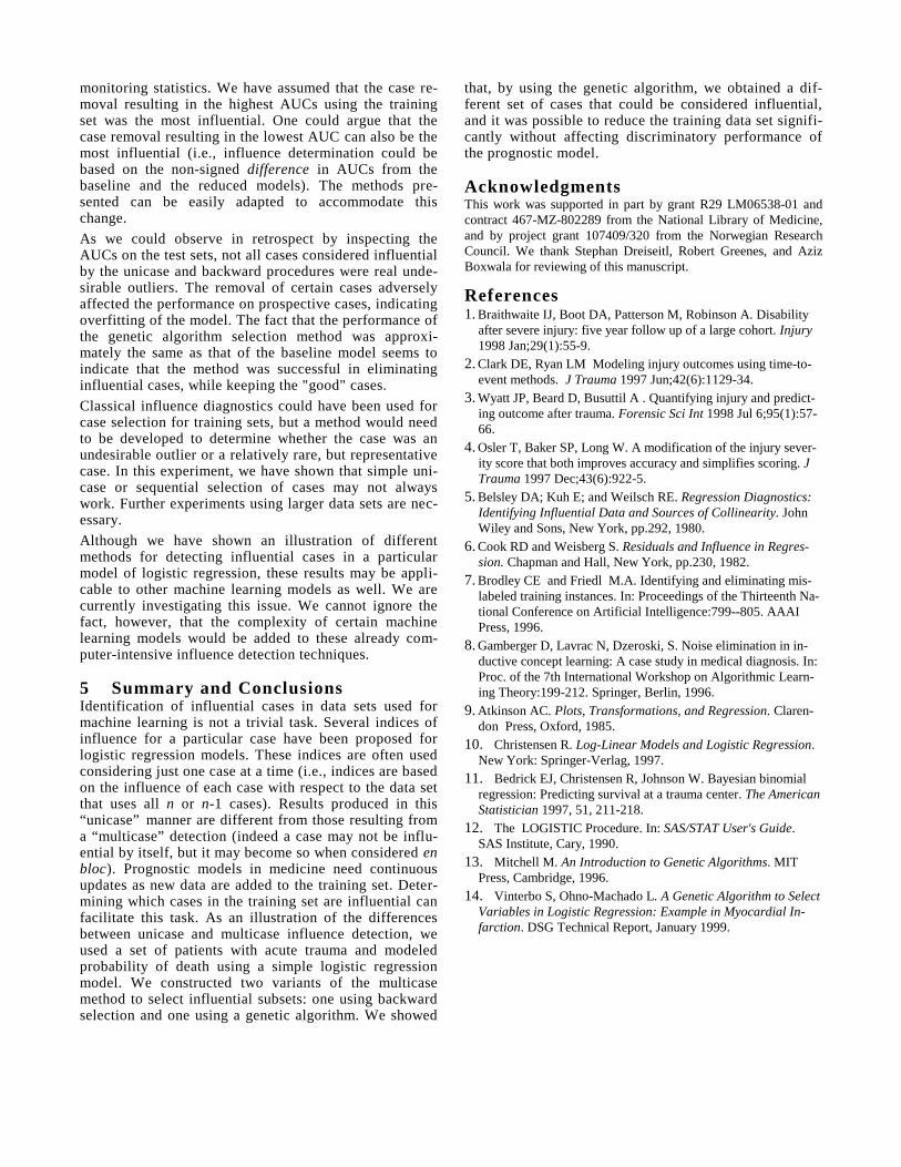
monitoring statistics. We have assumed that the case re-moval resulting in the highest AUCs using the trainingset was the most influential. One could argue that thecase removal resulting in the lowest AUC can also be themost influential (i.e., influence determination could bebased on the non-signed difference in AUCs from thebaseline and the reduced models). The methods pre-sented can be easily adapted to accommodate thischange.As we could observe in retrospect by inspecting theAUCs on the test sets, not all cases considered influentialby the unicase and backward procedures were real unde-sirable outliers. The removal of certain cases adverselyaffected the performance on prospective cases, indicatingoverfitting of the model. The fact that the performance ofthe genetic algorithm selection method was approxi-mately the same as that of the baseline model seems toindicate that the method was successful in eliminatinginfluential cases, while keeping the "good" cases.Classical influence diagnostics could have been used forcase selection for training sets, but a method would needto be developed to determine whether the case was anundesirable outlier or a relatively rare, but representativecase. In this experiment, we have shown that simple uni-case or sequential selection of cases may not alwayswork. Further experiments using larger data sets are nec-essary.Although we have shown an illustration of differentmethods for detecting influential cases in a particularmodel of logistic regression, these results may be appli-cable to other machine learning models as well. We arecurrently investigating this issue. We cannot ignore thefact, however, that the complexity of certain machinelearning models would be added to these already com-puter-intensive influence detection techniques.

5 Summary and ConclusionsIdentification of influential cases in data sets used formachine learning is not a trivial task. Several indices ofinfluence for a particular case have been proposed forlogistic regression models. These indices are often usedconsidering just one case at a time (i.e., indices are basedon the influence of each case with respect to the data setthat uses all n or n-1 cases). Results produced in this“unicase” manner are different from those resulting froma “multicase” detection (indeed a case may not be influ-ential by itself, but it may become so when considered enbloc). Prognostic models in medicine need continuousupdates as new data are added to the training set. Deter-mining which cases in the training set are influential canfacilitate this task. As an illustration of the differencesbetween unicase and multicase influence detection, weused a set of patients with acute trauma and modeledprobability of death using a simple logistic regressionmodel. We constructed two variants of the multicasemethod to select influential subsets: one using backwardselection and one using a genetic algorithm. We showed

that, by using the genetic algorithm, we obtained a dif-ferent set of cases that could be considered influential,and it was possible to reduce the training data set signifi-cantly without affecting discriminatory performance ofthe prognostic model.

AcknowledgmentsThis work was supported in part by grant R29 LM06538-01 andcontract 467-MZ-802289 from the National Library of Medicine,and by project grant 107409/320 from the Norwegian ResearchCouncil. We thank Stephan Dreiseitl, Robert Greenes, and AzizBoxwala for reviewing of this manuscript.

References1. Braithwaite IJ, Boot DA, Patterson M, Robinson A. Disability

after severe injury: five year follow up of a large cohort. Injury1998 Jan;29(1):55-9.

2. Clark DE, Ryan LM Modeling injury outcomes using time-to-event methods. J Trauma 1997 Jun;42(6):1129-34.

3. Wyatt JP, Beard D, Busuttil A . Quantifying injury and predict-ing outcome after trauma. Forensic Sci Int 1998 Jul 6;95(1):57-66.

4. Osler T, Baker SP, Long W. A modification of the injury sever-ity score that both improves accuracy and simplifies scoring. JTrauma 1997 Dec;43(6):922-5.

5. Belsley DA; Kuh E; and Weilsch RE. Regression Diagnostics:Identifying Influential Data and Sources of Collinearity. JohnWiley and Sons, New York, pp.292, 1980.

6. Cook RD and Weisberg S. Residuals and Influence in Regres-sion. Chapman and Hall, New York, pp.230, 1982.

7. Brodley CE and Friedl M.A. Identifying and eliminating mis-labeled training instances. In: Proceedings of the Thirteenth Na-tional Conference on Artificial Intelligence:799--805. AAAIPress, 1996.

8. Gamberger D, Lavrac N, Dzeroski, S. Noise elimination in in-ductive concept learning: A case study in medical diagnosis. In:Proc. of the 7th International Workshop on Algorithmic Learn-ing Theory:199-212. Springer, Berlin, 1996.

9. Atkinson AC. Plots, Transformations, and Regression. Claren-don Press, Oxford, 1985.

10. Christensen R. Log-Linear Models and Logistic Regression.New York: Springer-Verlag, 1997.

11. Bedrick EJ, Christensen R, Johnson W. Bayesian binomialregression: Predicting survival at a trauma center. The AmericanStatistician 1997, 51, 211-218.

12. The LOGISTIC Procedure. In: SAS/STAT User's Guide.SAS Institute, Cary, 1990.

13. Mitchell M. An Introduction to Genetic Algorithms. MITPress, Cambridge, 1996.

14. Vinterbo S, Ohno-Machado L. A Genetic Algorithm to SelectVariables in Logistic Regression: Example in Myocardial In-farction. DSG Technical Report, January 1999.

A specialised POMDP form and algorithmfor clinical patient management

Niels PeekDepartment of Computer Science, Utrecht University,P.O. Box 80.089, 3508 TB Utrecht, The Netherlands

E-mail: niels@cs.uu.nl

Abstract

Partially observable Markov decision pro-cesses (POMDPs) have recently been sug-gested as a suitable model to formalising theplanning of clinical patient management overa prolonged period of time. However, prac-tical application of POMDP models is ham-pered by the computational complexity of as-sociated solution methods. It is argued thatthe full generality of POMDPs is not neededto support many decision problems in clini-cal patient management, and that specialisedforms are often sufficient. A specialised formof POMDP, tailored to a particular type ofmanagement problem, is introduced. It is de-scribed how a new solution method, based onMonte Carlo simulations of the decision pro-cess, can take advantage of this specialisedform.

1 Introduction

Managing patients that suffer from a progressive dis-ease is a complicated task involving a mixture of testplanning, treatment selection, and prognostic assess-ment. The large number of possible managementstrategies over time precludes formalisation of thistask using traditional representations such as deci-sion trees and influence diagrams. Recently, partiallyobservable Markov decision processes (POMDPs) [4;8] have been suggested as a providing a suitable, in-tegrated approach to this type of management prob-lem [7; 10]. POMDPs are models for sequential deci-sion making under conditions of uncertainty and lim-ited observation opportunities. By taking into ac-count both immediate and longterm consequences ofdecisions, POMDPs provide a powerful framework fordecision-theoretic planning of clinical actions. Unfor-tunately, the computational burden associated withsolving POMDPs is overwhelming, precluding theirapplication to problems of practical size [9].

However, for many specialised problems, the full-blown generality of the POMDP approach and itsassociated solution methods is superfluous. We be-

lieve that this holds in particular for clinical decisionproblems, where often the class of admissible solu-tions is significantly constrained. In this paper, wediscuss a specialisation of POMDPs that is tailored toa frequently re-occurring type of clinical managementproblem, and propose a solution method that is ableto exploit the properties of this specialised form. Themanagement problem we envision to support looks asfollows. A patient suffers from a disease from whichnatural recovery is possible, but which may also causeharmful complications over time. There are possibil-ities to halt progress of the disease and its complica-tions by intervention (e.g. surgery), but these involvea serious risk to the patient. The main problem istherefore deciding whether or not to intervene, andif so, when. Prior to intervention, it is possible toperform several diagnostic procedures; these proce-dures reveal information on the clinical state of thepatient at the time the procedure is undertaken, butthey also comprise a (smaller) risk. A secondary prob-lem is therefore the selection and timing of diagnosticprocedures.

2 Model formIn this section, we briefly describe the generalPOMDP model and its associated solution form.Given a set X of variables, let ΩX denote the set ofall configurations of X , i.e. all possible value assign-ments to variables from X . A POMDP model is atuple (T, X, A, P, o, L), where• T is a linearly ordered set of decision moments,• X is a finite set of stochastic variables, jointly

defining the set ΩX of states,• A is a finite set of available actions,• P = pa

t : ΩX × ΩX → [0, 1] | a ∈ A, t ∈ T is a set of time- and action-dependent transitionprobability functions,

• o : A → ℘(X) is an observation function, and• L : lt : ΩX × A → R | t ∈ T is a set of time-

dependent loss functions.The set T of decision moments denotes the points intime where the decision maker is expected to select an

action a ∈ A. We restrict ourselves to finite-horizonproblems, and take T = 0, 1, 2, . . . , N ⊂ N. No ac-tion is selected at the last decision moment t = N ;this moment is included for evaluation of the finalstate only. The clinical state of the patient is de-scribed by the set X of discrete, stochastic variables;let S = ΩX × · · · × ΩX = ΩN+1

X denote the set of allpossible state sequences. When configuration c ∈ ΩX

characterises the state at time point t ∈ T , selectionof action a ∈ A will result in a transition to state c′at time point t + 1 with probability pa

t (c, c′). Fur-thermore, the decision maker is able to observe theconfiguration of the set o(a) ⊆ X at time point t, andcan use this observation to optimise subsequent deci-sion making; note that the observation function o isindependent of time. At each decision moment thedecision maker also incurs a loss lt(c, a); the losses as-sociated with subsequent moments in a realisation ofthe decision process are combined by a utility functionu : R

N+1 → R.Now, let φ be a joint probability distribution on

X at the initial time point t = 0, reflecting the deci-sion maker’s prior beliefs on the clinical state of thepatient. Given φ and a sequence α of action choicesfor all decision moments (except t = N), we obtain aprobability distribution on Prφ,α on the set S of pos-sible state sequences. From this distribution, we cancompute the expected utility of action sequence α un-der φ. Our objective is to select actions during the de-cision process such that expected utility is maximised.Prior to the first action choice, we therefore composea decision-theoretic plan π, which prescribes an actionchoice for each time point t < N , given the history ofpast actions and observations. When m is the max-imum number of distinct observations that may fol-low an action choice (i.e., if Y = o(a) then |ΩY | ≤ m,for each action a ∈ A), we have that mN is an up-per bound on the size decision-theoretic plans. Thenumber of possible plans is bounded by kmN , wherek = |A| is the number of available actions. It is there-fore not surprising that the problem of finding theoptimal plan is PSPACE-complete [9].

A POMDP model was recently developed to sup-port the clinical management of patients with ven-tricular septal defect (VSD), a frequently occurringcongenital heart disease [10]. A VSD is an abnormalopening in the heart causing heart failure and asso-ciated symptoms such as shortness of breath, feed-ing problems, and growth retardation. Approximately70% of all VSDs close spontaneously in the first yearsof life due to tissue growth, obviating the need forsurgical intervention. However, in the long run thedisease may cause irreversible damage to the lungsand a severely impaired respiratory function. Sev-eral diagnostic tests (ECG, echocardiography, cardiaccatheterisation, chest X-ray, and pulmonary biopsy)are available to examine the patient’s condition beforedeciding upon cardiac surgery. The cardiologist treat-ing a VSD patient therefore faces the type of man-

agement problem described in the previous section.The POMDP model for VSD has 33 state variables,yielding approximately 9, 7 · 1015 possible configura-tions (i.e. states of the POMDP); many configura-tions, however, cannot occur in practice, or can onlyoccur in specific circumstances. This is expressed inthe transition probability functions by assigning zeroprobability to those configurations. The model distin-guishes 6 decision moments (ages of the patient, rang-ing from 3 months to 8 years), and 7 distinct actionsto choose from.

It was also shown in [10] how temporal probabilis-tic networks can be used to graphically represent thetransition probability functions of a POMDP model,and how this representation, by exploiting conditionalindependence relations between state variables, canstrongly reduce the number of probability estimatesrequired to complete the model. This is especiallyuseful when the number of state variables is large: thecomplexity of transition probability functions quicklygrows in the number of variables. A compact repre-sentation, as in probabilistic networks, is then indis-pensable as obtaining probability estimates is often acumbersome task. We do not further elaborate on thisrepresentation here, and refer the interested reader tothe paper in question for more details.

3 A specialised POMDP formWe will now propose a special form of POMDP modelthat is tailored to support the management problemdescribed in Section 1. We first characterise the typesof loss and utility function that are used within thisspecial form, and then describe three restricting as-sumptions we make on actions, transition probabili-ties, and plan structure.

We take a loss lt(c, a), t < N , to represent themortality risk associated with state c and action aat time point t, and a loss lN(c′) to denote life ex-pectancy (in years) associated with final state c′ attime point t = N , where no action choice is made. Letr0, . . . , rN−1 be such mortality risks, obtained from agiven evolution of the decision process (i.e. states andactions for each of the decision moments up to timepoint t = N − 1). Then,

st =t−1∏

i=0

(1− ri) (1)

denotes the chance that the patient survives at leastup to time point t > 0. Now, let dt be the (fixed)actual duration (in years) between the start of thedecision process and decision moment t, 0 ≤ t ≤ N ;we then have that

let =t−1∑

j=1

djrjsj (2)

is the life expectancy of the patient up to time point t.The following utility function u now expresses overall

life expectancy:

u(r0, . . . , rN ) = leN + (dN + rN ) · sN , (3)

where rN = lN (c′) denotes life expectancy at the finaltime point. This type of utility function is generallyreferred to as risk-sensitive [5]. We note that it isalso possible to encode mortality risks in the transitionprobability functions, but we deliberately choose notto do so, for reasons explained shortly.

We make three further assumptions on the POMDPmodel and its admissible solutions. First, the set Ais taken to be composed of three disjoint sets Atest,Atreat, and Askip, where Atest constitutes the set ofavailable diagnostic procedures, Atreat lists treatmentalternatives, and Askip is a singleton set that consistsof the special action skip (i.e. refrain from acting atthe specified point in time) only. The set Atreat is as-sumed to be relatively small compared to Atest; e.g.,in the VSD domain, we have Atreat = surgery andAtest = ECG, echo, catheter ,X−ray, biopsy. Sec-ond, from Atreat an action is selected at most once, andafter that moment, further action is refrained from(by selecting skip for all subsequent moments). Be-fore the moment of treatment though, actions may beselected freely from Atest and Askip. From the firsttwo assumptions we thus obtain a restricted set Πof admissible plans, in each of which there is but asingle moment of control, preceded by multiple mo-ments of observation. The size of the set Π is boundedby (ktest + 1)mN , where ktest = |Atest|, and as before,m is the maximum number of distinct observationsthat may follow an action choice. Although ktest < k(where k = |A|), this number of admissible plans isstill very large. The average size of plans in Π, how-ever, equals mN/2.

The third and last assumption is that state devel-opment is independent of test actions. So, pa

t = pskipt

for each a ∈ Atest, t = 0, . . . , N − 1. Note that we canmake this assumption because mortality risks are en-coded in the loss functions: this enables us let all di-agnostic procedures induce the same transition prob-abilities, even if they differ with respect to their asso-ciated risks. Without this assumption, each of the kN

possible action sequences α induces a different proba-bility distribution Prφ,α on state sequences. With theassumption, many action sequences induce the samedistribution: we obtain (ktreat + 1)N classes of ac-tion sequences, ktreat = |Atreat|, where the sequencesin each class induce the same distribution. Action se-quences that are obtained from one of the admissibleplans in the set Π though, contain at most one actionchoice from Atreat. With that restriction, the numberof classes therefore further reduces to N · ktreat + 1.We will exploit this significant reduction in the solu-tion method described below.

4 Solution methodThe standard approach to solving POMDP problemswas initiated by Astrom [1] and Sondik [11], and is

based on transforming the POMDP into an equiva-lent, fully observable Markov decision process (calledthe belief MDP), over all possible probability distri-butions on the original state space ΩX . The beliefMDP can be solved using value iteration, a form ofdynamic programming [2]. However, the continuousstate space of the belief MDP is computationally dif-ficult to handle, and therefore the associated solutionalgorithms are complicated and limited [8]. Notwith-standing recent algorithmic advances in this field [3;6], solving POMDP problems of considerable size withthis approach seems to be infeasible; the current stateof the art allows to solve POMDPs with at most 10 to15 states. Another disadvantage of dynamic program-ming is that the decisions are optimised in reverse or-der. This implies that we cannot exploit prior knowl-edge of the problem involved (e.g. patient-specific in-formation), and it is difficult to take into account con-straints on plan structure, as for instance occur in thespecialised POMDP form described above. We there-fore propose a new solution method to solve POMDPs,tailored to the specialised form described above. Dueto space limitations, we restrict ourselves to giving asketch of the proposed method.

Basically, our method estimates expectations of theutility function u under a given decision-theoretic planπ ∈ Π by simulating the stochastic process on X un-der plan π. These Monte Carlo estimates are thencompared to establish the optimal plan. With thisapproach, we can easily exploit prior knowledge of theproblem case, as each simulation starts from the initialdecision moment; this is especially useful when manypotential state sequences are ruled out by the initialstate. Constraints on plan structure are taken intoaccount by selecting plans from the admissible set Πonly. Furthermore, we can take advantage of the factthat the distribution on state sequences is fixed bythe choice and timing of treatment. Let σ1, . . . , σn beindependent and identically distributed samples fromS, where treatment action a ∈ Atreat was selected attime point t < N in the simulations. Since the transi-tion probabilities are equal for all test actions and theskip action, we can use these samples to estimate ex-pectations of the function u for all action sequencesthat select treatment a at moment t, regardless oftheir prior testing policy. So, the simulation effortis strongly reduced as we evaluate a large variety ofaction sequences from a single collection of samples.

The space Π of admissible plans will generally betoo large to enumerate. We therefore perform a lo-cal search through Π, stepwise refining the plan underconsideration. The search process proceeds as follows.Let φ represent given beliefs on the initial state, andlet α be the action sequence where action a ∈ Atreat isselected at time point t < N , and skip is selected at allother times. Note that α also represents a (rather un-sophisticated) plan π ∈ Π: ‘perform action a at timepoint t without prior testing’. Now, let Prφ,α as beforebe the distribution on S induced by φ and α, and let

S be a collection of independent and identically dis-tributed samples from S drawn using Prφ,α. If u(σ, α)denotes the life expectancy associated with state andaction sequences σ and α, then

uφ,α(S) =1|S|

∑

σ∈S

u(σ, α) (4)

is an Monte Carlo estimate of life expectancy underplan π. To obtain more sophisticated plans, we nowtry to find indicators of variation in u. We say thatthe set Y ⊆ X is such an indicator at time pointt′ < t, if there exists configurations c′Y and c′′Y of Ysuch that difference between uφ,α(S′) and uφ,α(S′′) isstatistically significant, where S′, S′′ are the subcollec-tions of state sequences matching c′Y and c′′Y at timepoint t′, respectively. We restrict the search processto indicators Y that are observable, i.e. Y = o(a′) forsome action a′ ∈ Atest. Furthermore, the differencebetween estimated life expectancies must remain sig-nificant when adjusted for performing test action a′at time point t′. The plan π is now refined by addingthe test action corresponding to the indicator that in-duces the most significant difference in life-expectancyestimates. Subsequently, the treatment action and itstiming are re-considered for each of the possible ob-servations that may follow a′; new simulations maybe needed to obtain the necessary samples here. Af-ter possible adjustment of the treatment choice undereach of the observations, the process is repeated; pol-icy refinement is halted when no further improvementscan be found.

We note that Monte Carlo estimates converge tocorrect expected values in the limit of taking an in-finite number of samples. In practice, however, a fi-nite, and often small, number of samples is sufficient.Furthermore, the number of samples corresponding toparticular events is balanced with the likelihood ofthese events to occur. In our application of the tech-nique, this means that highly improbable state devel-opments are considered only after taking a large num-ber of samples. At the start of the policy-refinementprocess, improvements to the policy will be based ondevelopments that are either very likely to occur or in-duce large differences in life expectancy. As the refine-ment process proceeds and more samples are obtained,improvements may also be based on rare developmentsthat induce small differences.

5 Discussion and future work

POMDPs provide a powerful modelling framework fordecision-theoretic planning, with promising applica-tions to multi-stage clinical decision problems. Thegenerality of the standard POMDP model, however,limits practical application of the framework due tothe computational complexity of associated solutionmethods. To alleviate this obstacle, we have proposeda specialised POMDP form and algorithm to supporta frequently encountered type of clinical management

problem. The specialised form assumes several restric-tions on the effects of actions on state development,and on the structure of admissible solutions. These re-strictions jointly reduce the number of action-sequenceclasses that induce a different probability distributionon state sequences. Our algorithm exploits this prop-erty by reducing the simulation effort in Monte-Carloevaluation of decision-theoretic plans: each sample ofthe stochastic process is used to evaluate a large num-ber of action sequences.

We are currently implementing our algorithm, andplan to evaluate its performance on the VSD modelin the near future. Further research is required to in-vestigate extensions to the basic model form proposedhere. For instance, more elaborate loss and utilityfunctions that incorporate quality of life and costs oftreatment, are needed to provide a more realistic ac-count of the tradeoffs in real-world clinical decisions.Furthermore, allowing a larger number of control mo-ments is needed to support a wider range of manage-ment problems. To prevent a combinatorial explosionin the solution space, this extension should be copedto a fine-grained classification of action types and as-sociated restrictions on admissible treatment plans.

Acknowledgements

The investigations were (partly) supported by theNetherlands Computer Science Research Foundationwith financial support from the Netherlands Organisa-tion for Scientific Research (NWO). The author wishesto thank Jaap Ottenkamp for his support in construct-ing the VSD model.

References

[1] K.J. Astrom. Optimal control of Markov pro-cesses with incomplete state information. J.Math. Anal. Appl., 10:174–205, 1965.

[2] R.E. Bellman. Dynamic Programming. PrincetonUniversity Press, 1957.

[3] A.R. Cassandra, M.L. Littman, and N.L. Zhang.Incremental pruning: a simple, fast, exactmethod for partially observable Markov decisionprocesses. In Proc. 13th Conf. Uncertainty in Ar-tificial Intelligence (UAI–97), pp. 54–61, 1997.

[4] A.W. Drake. Observation of a Markov Processthrough a Noisy Channel. Ph.D. thesis, MIT,1962.

[5] E. Fernandez-Gaucherand and S.I. Marcus. Risk-sensitive optimal control of hidden Markov mod-els: Structural results. IEEE Trans. AutomaticControl, 42:1418–1422, 1997.

[6] M. Hauskrecht. Incremental methods for comput-ing bounds in partially observable Markov deci-sion processes. In Proc. 14th Nat. Conf. Artif.Intell. (AAAI–97), 1997.

[7] M. Hauskrecht and H. Fraser. Planning medicaltherapy using partially observable Markov deci-sion processes. In Proc. 9th Int. WS Principlesof Diagnosis (DX–98), pp. 182–189, 1998.

[8] W.S. Lovejoy. A survey of algorithmic methodsfor partially observed Markov decision processes.Ann. Oper. Res., 28:47–66, 1991.

[9] C.H. Papadimitriou and J.N. Tsitsiklis. The com-plexity of Markov decision processes. Math. Oper.Res., 12(3):441–450, 1987.

[10] N.B. Peek. Explicit temporal models for decision-theoretic planning of clinical management. Artif.Intell. Med., 15(2):135–154, 1999.

[11] E.J. Sondik. The Optimal Control of PartiallyObservable Markov Processes. Ph.D. thesis, Stan-ford University, 1971.

Robust Outcome Prediction for Intensive-Care Patients

Marco Ramoni

Knowledge Media Institute

The Open University

United Kingdom

Paola Sebastiani

Department of Statistics

The Open University

United Kingdom

Richard Dybowski

Intensive Care Group

King's College London

United Kingdom

Abstract

Missing data are a major plague of medicaldatabases in general, and of Intensive CareUnits (ICUs) databases in particular. Thetime pressure of work in an ICU pushes thephysicians to omit randomly or selectivelyrecord data. These dierent omission strate-gies give rise to dierent patterns of miss-ing data and the recommended approach ofcompleting the database using median impu-tation and tting a logistic regression modelcan lead to signicant biases. This paper ap-plies a new classication method, called ro-bust Bayes classier, that does not rely onany particular assumption about the patternof missing data and compares it to the tradi-tional median imputation approach using adatabase of 327 ICU patients.

1 Introduction

The primary role of intensive care units (ICUs) is tomonitor and stabilize the vital functions of patientswith life-threatening conditions. In order to aid ICUnurses and intensivists with this work, scoring systemshave been developed to express the overall state of anICU patient as a numerical value. ICU data sets of-ten have missing values. One suggestion as to whya patient attribute remains unrecorded is that an in-tensivist assumes the variable to be clinically normalon the basis of some other observation and, therefore,not worthy of conrmation. Although this clinical-normality assumption has been criticized [2], the mor-tality rate is higher in those patients with completedrecords. Since abnormal physiological values are asso-ciated with increased risk, it has been argued that thissupports the clinical-normality assumption. In addi-tion to this, we suspect that there are random omis-sions due to the pressure of work within an ICU; thus,it may be the case that the incompleteness of an ICUdata set is due to a mixture of dierent missing-datamechanisms. This situation motivates the investiga-tion presented in this paper. We compare a logisticregression model derived from imputed missing data

with a Bayesian classier using a robust Bayesian esti-mator [10] to handle missing data. The main characterof this robust Bayesian classier is its ability to learnand predict on the basis of incomplete data with noassumption about the missing data mechanism.

2 Prognostic Models

In this section we describe two prognostic models: lo-gistic regression and the Naive Bayesian Classier.

2.1 Logistic Regression Models

APACHE II [4] is a subjective linear combinationbased on demographic and physiological attributes,which increases as the state of a patient declines.In spite of its subjectivity, posterior probabilities ofa dened outcome have been estimated by havingAPACHE II as a logistic-regression covariate [3]. In1985 [7], APACHE II was replaced with the logistic re-gression model, in which the probability of a patientoutcome is modeled as a logit function of the attributevalues via the function

p(outcomejx) = (1 + exp[(w0 +mX

i=1

wixi)])1 (1)

The variable outcome is binary, corresponding to thetwo states alive or not while in ICU, the xi are at-tributes that, in the model in Equation 1, are notsupposed to interact, and the wi values are param-eters that can be estimated from available data, usingMaximum Likelihood estimators. Once the parame-ters wi are estimated from a data set of cases, themodel in Equation 1 can be used for prediction of apatient outcome, by selecting the outcome with thelargest probability, or for dening a number of objec-tive scoring systems, which have proved to performbetter than those obtained subjectively [1].

2.2 The Naive Bayes Classier

Outcome prediction can be transformed into a clas-sication task by regarding the regression covariatesas attributes of two alternative classes representingthe patient outcome. In this section, we will describe

the application of a Naive Bayes Classier (nbc) [6;9] to a ICU database. A nbc is a supervised classica-tion model that assumes the conditional independenceof the attributes given the class. We describe the nbcin the context of two classes, although the nbc canbe used more generally, when the number of classes isgreater than two.A nbc is dened by the marginal probabilities

fp1; p2g of the two classes and by the conditional prob-abilities fpijkg of each attribute value xik given eachclass cj . These probabilities can be easily estimatedfrom the data as relative frequencies or adjusted rela-tive frequencies to account for prior information, whenthe attribute are discrete variables. As the logistic re-gression model in Equation 1, the nbc can be usedto evaluate the probability of a class, given a set ofattribute values e = fx1k; :::; xmkg as

p(c1jek) =

Qm

i=1 pi1kp1Qm

i=1(pi1kp1 + pi2kp2): (2)

This probability is then used for predicting the out-come of a patient on the basis of his/her attributevalues or to dene some scoring system, as discussedin the previous section.

3 Missing Data

When some entries in the data set are reported as un-known, the estimation of the parameters wi in the lo-gistic regression model 1 and of the probabilities fpjgand fpijkg in the nbc can be done by using imputa-tion [8]. Imputation essentially consists of replacingthe unknown entries by some value generated froman imputation model that depends on the assumptionmade about the missing data mechanism. Here, wefollow the classication introduced by Rubin [12]:

Data are said to be missing completely at randomif the probability that an entry is missing in thedata set is independent of the other values, ob-served or not;

Data are said to be missing at random if the proba-bility that an entry is missing in the data set is afunction of the values observed in the data set;

Data are said to be informatively missing if the prob-ability that an entry is missing is a function of thevalues observed or not in the data set.

In the context of ICU data, the missing entries in thedata set are missing completely at random when theyare caused by random omissions, as for instance dueto work pressure. Data that are omitted due to theassumption of clinical normality can be described asbeing missing at random, because the intensivist as-sumes the omitted variables to be clinically normal onthe basis of some other observation and, therefore, notworth conrmation. This situation is dierent fromdeliberately omitting values that were measured. Thislast case would yield data that are informatively miss-ing.

The assumption about the missing data mecha-nism aects the way that either the logistic regressionmodel or the nbc are induced from the available data.When data are missing completely at random then thedata available are still a \representative sample", onthe whole. When data are missing at random, thenthe data available are a representative sample whentaken by groups. In both cases, the available dataare sucient to ll in | either deterministically orstochastically | the missing entries. When neitherof these two assumptions hold, their enforcement canintroduce severe bias, and a correct model buildingrelies on the knowledge of the process responsible forthe missing data. Sebastiani and Ramoni [13] provideexamples of the bias due to an indiscriminate use ofimputation.Clearly, the solution is to use the correct imputation

model, but this is not always possible because of lackof information about the process that caused missingdata. In the next section, we describe a method forrobust classication that does not require any specicmodel for the missing data mechanism.

4 Robust Classication

The robust Bayesian estimator introduced by Ramoniand Sebastiani [10] is a novel approach that allowsto estimate the probabilities fpijk ; pjg specifying thenbc without making any assumption about the miss-ing data mechanism. This feature seems to be the ap-propriate solution to the complexity of missing datamechanisms involved in ICU databases. This estima-tor is based on a new view of incomplete data: with noinformation on the pattern of missing data, an incom-plete data set can only constrain the set of estimatesthat can be induced from the database. Hence, the ro-bust Bayesian estimator returns probability estimatesthat are robust with respect to the missing data mech-anism by providing probability intervals that containthe estimates learned from all possible completions ofthe incomplete database. The calculation of these in-terval estimates is done very eciently by computingvirtual frequencies that correspond to extreme com-pletions of the incomplete data. Compared to impu-tation, the robust Bayesian estimator does not rely ona single model for the missing data, but provides setsof estimates consistent with all possible missing datamechanisms from which the incomplete data at handcould have been obtained.However, in order to use the estimates computed

by the robust Bayesian estimator to produce a robustprognostic model, we need to nd a solution to thefollowing problems:

1. the evaluation of the posterior probability inEquation 2 requires the probabilities fpijk; pjg tobe point valued;

2. the use of intervals prevents the use of the stan-dard criterion of selecting the class with the high-est posterior probability, because the posterior

probabilities are intervals rather than single val-ues.

Ramoni and Sebastiani [11] describe an exact algo-rithm for extending Equation 2 to probability inter-vals. The algorithm maintains the same computa-tional complexity needed to evaluate Equation 2 andreturns, for each conditional probability p(cj je), prob-ability intervals [pmin(cj je); pmax(cj je)] that containall the values we would obtain from the possible com-pletions of the data.We now need a method for ranking probability in-

tervals, so that the prediction can be done by choos-ing the class associated with the highest ranked in-terval. The stochastic dominance criterion, proposedby Kyburg [5], predicts the class cj if and only if theminimum posterior probability of this class is higherthan the maximum posterior probability of the otherclasses. Stochastic dominance is the safest and mostconservative criterion, as it is independent of the miss-ing data mechanism. However, this criterion is unableto classify cases when intervals are overlapping and wetherefore have to resort to a weak dominance criterion.Weak dominance summarizes each probability inter-val into a point, called a robust classication score.The score is computed by assuming a uniform dis-tribution over the missing data, and the prediction isdone by selecting the class associated with the highestscore. More formally, by letting q denote the numberof classes, we dene the robust classication score ofcj je as

su(cj je) =pmin(cj je)(q 1)

q+

pmax(cj je)

q

When there are two classes, as in the present situation,the score su(cj je) is the interval mid-point. We notethat, in using a uniform distribution over the inter-val values, we are not assuming that data are missingcompletely at random. The latter condition would re-quire to weight each maximum probability pmax(cj je)by the probability pj that an unobserved entries of Cis cj .We dene a nbc that is induced from incomplete

data using the robust Bayesian estimator, and thatis used for classication using either stochastic domi-nance or weak dominance, the robust Bayes classier.The programRoC1, implements the robust Bayes clas-sier.

5 Experimental Evaluation

This section reports an experimental comparison on aICU database between a logistic regression model andthe robust Bayes classier. We rst describe the dataset and the procedure used compare the two models.

1available at http://kmi.open.ac.uk/projects/bkd

5.1 Material and Methods

The 327 patients comprising the data set were presentin the adult ICU at St Thomas' Hospital, London,from January 1997 to July 1997. The 11 variablesin the data set are listed in Table 1, and the valuesare those recorded during the rst 24-hours of eachpatient's stay in ICU. The data set is incomplete, ofthe 11 327 cells of the data set, 75 (2%) are empty,resulting in 67 (20%) incomplete rows.Contrary to the robust Bayes classier that does not

need any assumption about the missing data mecha-nism, the estimation of the parameters wi of the lo-gistic regression model relies on some explicit modelfor the missing data to allow for imputation. We im-puted the missing entries in the data set, under theassumption that data were missing completely at ran-dom. Hence, the missing entries of each covariatewere replaced by a reference value computed from themarginal distribution of the covariate itself. Since thecovariates have skewed distributions, we replaced themissing entries by the observed median of each vari-able, that is less sensitive to outliers.The comparison of predictive accuracy of the two

models was carried out by running ten replicates of a5-fold cross validation experiment. In each replicate,we divided the data set in 5 mutually exclusive datasets D1; :::;D5 of approximately the same size. Foreach data set Di, we estimated both the logistic re-gression model and the robust classier on the dataset D in which we removed the cases in Di and wethen used the two models to predict the outcome ofpatients in Di.

Estimation Each logistic regression model was es-timated using the S-Plus glm function with the ar-gument family=binomial. In each case, we ttedadditive logistic regression models without employinginteraction terms. Each robust Bayes classier was es-timated using the program RoC that implements therobust classication described in Section 4. Continu-ous variables were discretized in four equally spacedintervals of the logarithmic transformation of the ob-served values.

Prediction For this study, a patient is classiedas not surviving in hospital if his/her posteriorprobability for death while in hospital is greater than0.5 according to the logistic regression model. Onthe other hand, the robust Bayes classier underthe strong dominance criterion classies a patientas not surviving if the minimum probability of notsurviving is larger than the maximum probability ofsurviving. The robust Bayes classier under the weakdominance criterion predicts the patient outcome asthat one corresponding to the probability intervalwith largest mid-point.

As each data set Di contains the observed out-come, we evaluate the performance of the two models

Table 1: The attributes of interestVariable name Data type CodeAge (years) Continuous |Articial ventilation required Nominal \1" = true; \2" = falseType of inotrope support Ordinal \0" = no intotropes; \1" =

dopamine; \2" = adrenalineonly; \3" = adrenaline plusother inotrope(s)

Serum bilirubin (mmol/l) Continuous |Acute renal failure Nominal \1" = true; \2" = false24-h urine volume Ordinal \0" = (0 - 50ml); \1" = (51 -

300ml) ; \2" = (> 300ml)Surgical category Nominal \1" = elective (mostly car-

diothoracic); \2" = emergency(medical patients); \3"= emer-gency (general surgery)

Creatinine Continuous |Left ventricular intercept Continuous |Glasgow coma score Ordinal 1,2,...,15Alive whilst in hospital Nominal \1" = true; \2" = false

by comparing their predictive accuracy and coverage.The predictive accuracy measures the predictive qual-ity as the average number of cases that were correctlyclassied in the test sets. The coverage is the ratiobetween the number of cases classied and the totalnumber of cases in the data set. Hence, the coverageof the logistic regression model is 100%, as well as thecoverage of the robust Bayes classier that uses therobust classication score. The coverage of the robustBayes classier that uses the stochastic dominance cri-terion is the ratio between the number of cases thatwere classied and the size of the data set. Since thecross validation procedure was repeated 10 times, theclassication accuracy and coverage are computed asaverage values of the resulting 10 measures of accuracyand coverage, and we also provide 95% condence lim-its.

5.2 Results

The average classication accuracy of the logistic re-gression model was 80.25% 2:15. The classica-tion accuracy of the robust Bayes classier that usesthe stochastic dominance criterion increases to 85.4%2:05. The price of such increased accuracy is a de-creased coverage of 87.76% 2:06. Using the weakdominance criterion, we increased the coverage of therobust Bayes classier to 100% by reducing the accu-racy to 80.70% 2:15. Hence, compared to logisticregression, the gain of accuracy is 0.5%.

6 Conclusions

A conservative approach, with no commitment to aparticular missing data mechanism, improves the pre-dictive accuracy in our example data set but leavesunclassied a quota of the cases. When we increasethe coverage by adopting weaker criteria, the accuracy

reduces to a level comparable to the accuracy achievedby logistic regression with median imputation. Thesendings suggest that, in practical applications, a con-servative approach can be taken in order to increasethe accuracy of the predictions. The unclassied casescan be left for more careful consideration to a humanexpert, possibly aided by the predictions obtained un-der weaker criteria.Furthermore, the fact that, even under stochastic

dominance, the accuracy is limited to 85.4% 2:05questions the ability of the models considered to rep-resent the real dependence of the outcome variable onthe 10 attributes recorded in the data set. However,building improved logistic regression models from theincomplete data can be seriously biased by the impu-tation method adopted. The robust Bayes classiercan be improved by selecting relevant attributes onthe basis of their predictive relevance, without makingassumptions on the missing data mechanism. Prelim-inary results seem to suggest that a careful selectionof attributes having a signicant predictive relevancecan further increase the accuracy of the robust Bayesclassier.

Acknowledgements

This research was supported by the ESPRIT pro-gramme of the Commission of the European Commu-nity under contract EP29105 and by equipment grantsfrom Apple Computers and Sun Microsystems.

References

[1] X. Castella, A. Artigas, J. Bion, A. Kari, andThe European/North American Severity StudyGroup. A comparison of severity of illness scor-ing systems for intensive care unit patients: Re-

sults of a multicenter, multinational study. Crit-ical Care Medicine, 23:13271332, 1995.

[2] H.R. Champion and W.J. Sacco. Measurementof patient illness severity. Critical Care Medicine,10:552553, 1982.

[3] R.W.S. Chang, S. Jacobs, and B. Lee. Useof APACHE II severity of disease classica-tion to identify intensive-care-unit patients whowould not benet from total parenteral nutrition.Lancet, 1986i:14831487, 1986.

[4] W.A. Knaus, E.A. Draper, D.P. Wagner, and J.E.Zimmerman. APACHE II: A severity of diseaseclassication system. Critical Care Medicine,13:818829, 1985.

[5] H.E. Kyburg. Rational belief. Behavioral andBrain Sciences, 6:231273, 1983.

[6] P. Langley, W. Iba, and K. Thompson. Ananalysis of Bayesian classiers. In Proceedingsof the National Conference on Articial Intelli-gence, pages 223228, San Mateo, CA, 1992. Mor-gan Kaufman.

[7] S. Lemeshow, D.Teres, H. Pastides, J.S. Avrunin,and J.S. Steingrub. A method for predicting sur-vival and mortality of ICU patients using objec-tively derived weights. Critical Care Medicine,13:519525, 1985.

[8] R.J.A. Little and D.B. Rubin. Statistical Analysiswith Missing Data. Wiley, New York, 1987.

[9] S.G. Pauker, G.A. Gorry, J.P. Kassirer, and W.B.Shwartz. Toward the simulation of clinical cogni-tion: Taking a present illness by computer. TheAmerican Journal of Medicine, 60:981995, 1976.

[10] M. Ramoni and P. Sebastiani. Robust learningwith missing data. Technical Report KMi-TR-28,KMI, The Open University, 1996. Available athttp://kmi.open.ac.uk/techreports/KMi-TR-28.

[11] M. Ramoni and P. Sebastiani. Robust Bayesclassiers. Technical Report KMi-TR-82, KMI,The Open University, 1999. Available athttp://kmi.open.ac.uk/techreports/KMi-TR-82.

[12] D.B. Rubin. Inference and missing data.Biometrika, 63:581592, 1976.

[13] P. Sebastiani and M. Ramoni. Model folding fordata subject to nonresponse. In Proceedings ofArticial Intelligence and Statistics 1999, pages287292.Morgan Kaufman, San Mateo CA, 1999.

Prognoses for Multiparametric Time Courses of the Kidney Function

Rainer Schmidt a, Bernhard Pollwein b, Lothar Gierl a

a) Institute for Medical Informatics and Biometry, University of Rostock, Rembrandtstr. 16/17, 18055 Rostock, Germany,e-mail: rainer.schmidt@medizin.uni-rostock.de

b) Department of Anaesthesiology of the Ludwig-Maximilians University, Munich, Germany

Abstrac t

In this paper, we describe an approach to utilize Case-Based Reasoning (CBR) methods for trend prognoses for medicalproblems. Since using conventional methods for reasoning over time does not fit for course predictions without medicalknowledge of typical course pattern, we have developed abstraction methods suitable for integration into our Case-BasedReasoning system ICONS. These methods combine medical experience with prognoses of multiparametric courses. We havechosen the monitoring of the kidney function in an Intensive Care Unit (ICU) setting as an example for diagnostic problems.On the ICU, the monitoring system NIMON provides a daily report based on current measured and calculated kidney functionparameters. We subsequently generate course-characteristic trend descriptions of the renal function over the course of time.Using Case-Based Reasoning retrieval methods, we search in the case base for courses similar to the current trend descriptions.Finally, we present the current course together with similar courses as comparisons and as possible prognoses to the user. Weapplied CBR methods in a domain which seemed reserved for statistical methods and conventional temporal reasoning.

1. Introduction

Up to 60% of the body mass of an adult person consists ofwater. The electrolytes dissolved in body water are of greatimportance for an adequate cell function. The human bodytends to balance the fluid and electrolyte situation. Butintensive care patients are often no longer able to maintainadequate fluid and electrolyte balances themselves due toimpaired organ functions, e.g. renal failure, or medicaltreatment, e.g. parenteral nutrition of mechanicallyventilated patients. The physician therefore needs objectivecriteria for the monitoring of fluid and electrolyte balancesand for choosing therapeutic interventions as necessary.At our ICU, physicians daily get a printed renal reportfrom the monitoring system NIMON [1] which consists of13 measured and 33 calculated parameters of those patientswhere renal function monitoring is applied. For example,the urine osmolality and the plasma osmolality aremeasured parameters that are used to calculate the osmolarclearance and the osmolar excretion. The interpretation ofall reported parameters is quite complex and needs specialknowledge of the renal physiology.The aim of our knowledge based system ICONS is to givean automatic interpretation of the renal state to elicitimpairments of the kidney function on time. That means,we need a time course analysis of many parameters withoutany well-defined standards. At first glance, this seemed tobe a field to apply statistical methods. However, our goodresults of experiments with a Case-Based Reasoningapproach and our investigations of the difficulties to handlemultiparametric time course problems without a medical

domain theory revealed that CBR methods are moreapplicable in this field. Although much research has beenperformed in the field of conventional temporal courseanalyses in the recent years, none of them is suitable forthis problem. Allen‘s theory of time and action [2] is notappropriate for multiparametric course analysis, becausetime is represented as just another parameter in therelevant predicates and therefore does not give necessaryexplicit status [3]. As traditional time series techniques[4] with known periodicities work well unless abruptchanges, they do not fit in a domain characterized bypossibilities of abrupt changes and a lack of well-knownperiodicities at all. One ability of RÉSUMÉ [5] is theabstraction of many parameters into one single parameterand to analyse the course of this abstracted parameter.However, the interpretation of the courses requirescomplete domain knowledge. Haimowitz and Kohane [6]compare many parameters of current courses with well-known standards. In VIE-VENT [7] both ideas arecombined: Courses of quantitative measured parametersare abstracted into qualitative course descriptions, whichare matched with well-known standards.However, in the domain of fluid and electrolyte balance,neither a prototypical approach in ICU settings is knownnor exists complete knowledge about the kidneyfunction. Especially, knowledge about the behaviour ofthe various parameters over time is yet incomplete. Sowe had to design our own method to deal with courseanalyses of multiple parameters without prototypicalcourses and without a complete domain theory (Figure1).

State Abstraction: daily decision for one kidney function state

7 days course of states

Time Abstraction: generation of trends

Trend description

Presentation: current course andsimilar courses with continuations

CBR - Retrieval

parameters- 7th day

parameters - 1st day

parameters- 2nd day

state - 1st day state - 2nd day state - 7th day

Figure 1 - Abstractions for MultiparametricPrognoses in ICONS

2. Methods

2.1. General Model

Our procedure for interpretation of the kidney functioncorresponds to a general linear model. First, once a day themonitoring system NIMON gets 13 measured parametersfrom the clinical chemistry and calculates 33 meaningfulkidney function parameters. To elicit the relationshipsamong these parameters a three dimensional presentationability was implemented inside the renal monitoringsystem NIMON. However, complex relations among allparameters are not visible.We decided to abstract these parameters. For this dataabstraction we use states of the renal function whichdetermine states of increasing severity beginning with anormal renal function and ending with a renal failure. Basedon these state definitions, we determine the appropriatestate of the kidney function per day. Therefore, we presentthe possible states to the user sorted according to theirprobability. The physician has to accept one of them.Based on the transitions of the states of one day to the stateof the following day, we generate four different trends.These trends, which are abstractions of time, describe the

courses of the states. Then we use Case-Based Reasoningretrieval methods [8, 9, 10, 11] to search for similarcourses. We present similar courses together with thecurrent one as comparisons to the user, the coursecontinuations of the similar courses serve as prognoses.As there may be too many different aspects between bothpatients, the adaptation of the similar to the currentdevelopment is not done automatically. ICONS offersonly diagnostic and prognostic support, the user has todecide about the relevance of all displayed information.When presenting a comparison of a current course with asimilar one, ICONS supplies the user with the ability toaccess additional renal syndromes and the development ofsingle parameter values during the relevant time period.

2.2. Determination of the Kidney Function State

Based on the kidney function states, characterized byobligatory and optional conditions for selected renalparameters, first we check the obligatory conditions. Foreach state that satisfies the obligatory conditions wecalculate a similarity value concerning the optionalconditions. We use a variation of Tversky 's [8] measureof dissimilarity between concepts. If two or more statesare under consideration, ICONS presents these statessorted to the similarity values together with informationabout the satisfied and not satisfied optional conditions(Figure 2).The user can accept or reject a presented state. When asuggested state has been rejected, ICONS selects anotherstate. The choice depends not only on the computedsimilarity value, but also on previous decisions of theuser and the relation between the states. The states areordered according to the grade of renal impairment, e.g. itis not necessary to present the state "reduced kidneyfunction", if the user has already accepted the state"sharply reduced kidney function". Finally, we determinethe central state of occasionally more than one states theuser has accepted. This central state is the closest onetowards a kidney failure. Our intention is to find thestate indicating the most profound impairment of thekidney function.

2.3. Course-characteristic Trend Descriptions

First, we have fixed five assessment definitions for thetransition of the kidney function state of one day to thestate of the following day. These assessment definitionsare related to the grade of renal impairment:

steady: both states have the same severity value.increasing: exactly one severity step in the direction towards a normal function.

sharply increasing: at least two severity steps in the direction towards a normal function.decreasing: exactly one severity step in the direction towards a kidney failure.sharply decreasing: at least two severity steps in the direction towards a kidney failure.

These assessment definitions are used to determine the statetransitions from one qualitative value to another.Neighbouring state transitions with the same assessmentare combined into trend pieces. Based on these trend pieces,

we generate three trend descriptions. Two trenddescriptions especially consider the current statetransitions. The first trend description T1 is equivalent tothe current trend piece, the second trend description T2looks recursively back from the current trend piece to theone before and unites them, if they are both of the samedirection or one of them has a "steady" assessment. Athird trend description T3 characterizes the wholeconsidered course of at most seven days. In addition tothe five former assessment definitions we introduced fournew ones.

Figure 2 - Presentation of a current kidney function state estimated as reduced kidney function

If none of the five former assessments fits the complete considered course, we attempt to fit one of these four definitions in the following order:

alternating: at least two up and two down transitions and all local minima are equal.oscillating: at least two up and two down transitions.fluctuating: the distance of the highest to the lowest severity state value is greater than 1. nearly steady: the distance of the highest to the lowest severity state value equals one.

A fourth trend description T4 assesses the complete

considered course with a quantitative value that expressesthe average number of state transition values inverselyweighted by the distance to the current day.Looking back from a time point t, these four trenddescriptions form a pattern of the immediate coursehistory of the kidney function considering qualitative andquantitative assessments.

2.4. Retrieval

We use the parameters of the four trend descriptions andthe current kidney function state to search for similarcourses (a retrieval result is depicted in Figure 3). As the

aim is to develop an early warning system, we need aprognosis. For this reason and to avoid a sequentialruntime search along the whole cases, we store a course ofthe previous seven days and a maximal projection of threedays for each day a patient spent on the ICU.As there are many different possible continuations for thesame previous course, it is necessary to search for twoitems: Similar courses and different projections.Therefore, we divided the search space into nine partscorresponding to the possible continuation directions.Each direction forms an own part of the search space.During the retrieval these parts are searched separately andeach part may provide at most one similar case. Thesimilar cases of these parts together are presented in theorder of their computed similarity values.Before the main retrieval, we search for a prototype thatmatches most of the trend descriptions. Below thisprototype the main retrieval starts. It consists of twosteps for each part. First we search with an activation

algorithm concerning qualitative features. Our algorithmdiffers from the common spreading activation algorithm[9] mainly due to the fact that we do not use a net for thesimilarity relations. Instead, we have defined explicitactivation values for each possible feature value. This ispossible, because on this abstraction level there are onlyten dimensions with at most six values.Subsequently, we check the retrieved cases with anadaptability criterion [10], which looks for sufficientsimilarity, since even the most similar course may differfrom the current one significantly. This may happen atthe beginning of the use of ICONS, when there are only afew cases known to ICONS, or when the current course israther exceptional. Because of the lack of medicalknowledge about sufficient similarity, we defined aminimal similarity criterion that may be improved aftersome experience with ICONS.

Figure 3 - Screendump of a comparative presentation of a current and a similar course. In the lower part of eachcourse the (abbreviated) kidney function states are depicted. The upper part of each course shows the deduced trenddescriptions.

If several courses are selected in the same projection part,we use a sequential similarity measure concerning thequantitative features in a second step. This measure is avariation of TSCALE [11] and goes back to Tversky [8].

2.5. Learning a Tree of Prototypes

Prognosis of multiparametric courses of the kidneyfunction for ICU patients is a domain without a medicaltheory. Moreover, we can not expect such a theory to beformulated in the near future. So we attempt to learnprototypical course pattern. Therefore, knowledge on thisdomain is stored as a tree of prototypes with three levelsand a root node. Except for the root, where all not yetunited courses are stored, every level corresponds to one ofthe trend descriptions T1, T2 or T3. As soon as enoughcourses that share another trend description are stored at aprototype, we create a new prototype with this trend. At aprototype at level 1, we unite courses that share T1, atlevel 2, courses that share T1 and T2 and at level 3,courses that share all three trend descriptions. We can dothis, because regarding their importance, the three trenddescriptions T1, T2 and T3 refer to hierarchically relatedtime periods. T1 is more important than T2 and T3.We start the retrieval with a search for a prototype thathas most of the trend descriptions with the current coursein common.

2.6. Evaluation

To verify the knowledge base we selected 100 data setsfrom the NIMON database. The selection was only partlyat random, because we wanted adequate representation ofall kidney function states. Two physicians experiencedwith the kidney function were asked to classify theselected data sets according to the concepts, but withoutknowing ICONS`s obligatory and optional conditions ofthe kidney function states. We compared the results ofthe physicians with ICONS`s classifications of the samedata sets. The comparison was mostly satisfactory. For 83parameter sets the classifications of ICONS correspondedto those of the physicians. In 16 cases ICONS tendedmore towards the direction of kidney failures. Only onceICONS classified the parameter set as a "reduced kidneyfunction" while the physicians assessed it as a "kidneyfailure". However, as a result of the evaluation weslightly modified the state definition of the "reducedkidney function".

3. Conclusion

Our aim is to produce an early warning system that helpsto avoid kidney failures. ICONS helps the physicians toabstract from the measured and calculated NIMON

parameters to a function state. For time periods up toseven days, we describe courses of function states usingfour trend descriptions as a second abstraction step. Atthis double abstraction level, ICONS provides thephysicians with courses of other patients with similardevelopments as potential warnings. As no prototypicalcourses towards a kidney failure are known, we search forcases with similar courses and present them as possibleprognoses. We hope to find some prototypical courses bymerging similar courses into prototypes. One advantageof combining temporal course analyses with Case-BasedReasoning is the projection. Without medical knowledgeabout possibilities and probabilities of futuredevelopments ICONS shows future developments ofpatients with similar courses.

References[1] U. Wenkebach, B. Pollwein, U. Finsterer, " Visualizationof large datasets in intensive care", in: Proc Annu SympComput Appl Med Care, 1992, pp. 18-22[2] J.P. Allen, "Towards a general theory of action and time",Artificial Intelligence Vol. 23, 1984, pp. 123-154[3] E.T. Keravnou E.T., "Modelling Medical Concepts asTime Objects", in: P. Barahona, M. Stefanelli, J. Wyatt(Eds.): Artificial Intelligence in Medicine, AIME‘95, Berlin,1995, pp. 67-78[4] S.M. Robeson, D.G. Steyn, "Evaluation and comparisonof statistical forecast models for daily maximum ozoneconcentrations", Atmospheric Environment, Vol. 24 B, No.2, 1990, pp. 303-12[5] Y. Shahar, M.A. Musen, "RÉSUMÉ: A Temporal-Abstraction System for Patient Monitoring", Computers andBiomedical Research, Vol. 26, 1993, pp. 255-273[6] I.J. Haimowitz, I.S. Kohane, "Automated Trend Detectionwith Alternate Temporal Hypotheses", in: R. Bajcsy (ed.),Proceedings of the 13th International Joint Conference onArtificial Intelligence (IJCAI-93), Morgan Kaufmann, SanMateo, CA, 1993, pp. 146-151[7] S. Miksch, W. Horn, C. Popow, F. Paky, "TherapyPlanning Using qualitative Trend Descriptions", in: P.Barahona, M. Stefanelli, J. Wyatt (Eds.): ArtificialIntelligence in Medicine, Springer Berlin, 1995, pp. 197-208[8] A. Tversky, "Features of Similarity", PsychologicalReview, Vol. 84 , 1977, pp. 327-352[9] J.R. Anderson, "A theory of the origins of humanknowledge", Artificial Intelligence, Vol. 40, Special Volumeon Machine Learning, 1989, pp. 313-351[10] B. Smyth, M.T. Keane M.T., "Retrieving AdaptableCases: The Role of Adaptation Knowledge in Case Retrieval"in: First European Workshop on Case-Based Reasoning(EWCBR-93), 1993, pp. 76-81[11] W.S. DeSarbo, M.D. Johnson, A.K. Manrei, L.A.Manrai, E.A. Edwards, "TSCALE: A new multidemensionalscaling procedure based on Tversky's contrast model",Psychometrika, Vol. 57, 1992, pp. 43-69

AbstractChildren and adolescents referred to clinical ex-aminations due to the loss of consciousness, fallsor other paroxysmal motor phenomena are fre-quently incorrectly diagnosed as epileptic. It isextremely important to avoid incorrect diagnosisof epilepsy, not only because of the stigma at-tached to the label `epileptic’ but also due tofrequent side-effects of anti-epileptic drugswhich should not be given to patients who can-not benefit from their use. An expert such as anexperienced pediatric neurologist is able tomake correct diagnosis by a detailed history ex-amination. Since expert neurologists are not al-ways available, we tried to model such expertknowledge by the use of machine learning ondata collected from the history of 72 patients: 44patients having first epileptic seizure and 28 pa-tients having syncope. The induced decision treesuggests a stepwise diagnostic process using justfew decisive data entries obtained from the his-tory of the event, resulting in 90% accurate di-agnosis of either first epileptic seizure or syn-cope, with 86% specificity and 93% sensitivity.Using such a decision tree model in practicewould provide great help and would result in amuch more accurate diagnostic procedure thanthe rather ill-defined procedures used by inexpe-rienced doctors. Moreover, correct diagnosismade on the basis of history data may help toavoid many further unnecessary investigations.When the machine induced expert knowledge isused as a prognostic model, the syncope out-come means a great relief to the patient, sincesyncope can easily be prevented by simplemeasures. On the other hand, the case of epi-leptic fit prognosis requires a cautious approachwith some predictive measures and guidelinesabout everyday life.

Keywords: Machine learning, decision tree induction,cerebral paroxysm, epileptic seizure, syncope

1 IntroductionThe term epileptic seizure refers to a sudden change inthe electrical activity of the brain, usually accompaniedby subjective or objective changes of behavior, motoractivity, posture etc. Epilepsy is a condition with recur-rent unprovoked seizures or, in some cases, provokedonly by everyday stimuli. Non-epileptic seizures are sud-den changes in behavior which are not due to an inde-pendent sudden change in the electrical activity of thebrain, but are due to a sudden change (drop) of bloodflow through the brain; these are also named anoxic(without oxygen) seizures. Non-epileptic seizures can bedivided into physiological non-central nervous systemevents, such as syncope, toxic and psychogenic seizures,etc. The most frequent and still too many times misdiag-nosed as epileptic fit are syncopes (fainting fits), whichusually begin with sudden fall and are also often quitedramatic, associated with convulsions and incontinence,which may misleadingly suggest epileptic seizure.Everyday clinical experience in outpatient clinic and inhospitals indicate that the most difficult problem is thedistinction between anoxic and epileptic seizure, betweenfainting fits and epileptic fits, when the first event issudden fall.The diagnosis of cerebral paroxysmal disor-ders (fits or faints) is based on detailed patient’s history.The objective is to elicit a sequence of events as de-scribed by a patient and by a witness, circumstances ofthe event, stimulus, onset, duration of unconsciousnessand immediate postictal course. The goal of a rationaldiagnostic algorithm is to establish the final diagnosisand to offer the patient an appropriate treatment. Onlyfew investigations are necessary, depending on the syn-cope or epilepsy diagnosis. If the later is the case, moreinvestigations will follow; therefore correct diagnosis,which is based on detailed and reliable patient’s historyis a very important starting point.

Impact of Machine Learning to the Diagnosis and Prognosis of First CerebralParoxysm

Igor Zeliþ1DGD/DYUDþ Peter Najdenov, Zvonka Rener-PrimecDepartment of Intelligent Systems

Jozef Stefan InstituteJamova 39, 1000 Ljubljana, Slovenia

e-mail: igor.zelic@ijs.si, nada.lavrac@ijs.si

Department of Child NeurologyUniversity Medical Center,

Children Hospital,Vrazov trg 1, 1000 Ljubljana, Slovenia

e-mail: peter.najdenov@guest.arnes.si,zvonka.rener@mf.uni-lj.si

Clinical features in anoxic seizures are usually recordedin the following sequence: subjective feeling of light-head, blurred vision or darkness in front of the eyes (butcan still hear voices), pale, cold skin, atonia or limpness(sudden fall), stiffening, jerks, disorientation, inconti-nence. When signs and symptoms of the event are cor-rectly asked and given by detailed history, an expert (likean experienced pediatric neurologist) is able to make acorrect diagnosis from the history data alone. In ourstudy we used medical data about patients admitted tothe Children Hospital of Ljubljana in 1997-1998 for thediagnosis of the first paroxysmal event. Out of 72 pa-tients, 44 had first epileptic seizure and 28 patients hadsyncope. Each patient record consisted of values of 23attributes, including subjective symptoms just before theevent (blurred vision or darkens in front of eyes, suddenfall from vertical position, stiffening, limpness, change inskin color, change of position before seizure) and afterevent sings (headache, vomiting after episode, long sleepor normal activity), number of previous seizures, time torecover, …

2 Data analysis toolsIn this study two machine learning data analysis toolswere used: a decision tree learner Magnus Assistant andthe Naive Bayesian classifier.

2.1 Magnus AssistantMagnus Assistant [Mladeniü ] is a descendant ofAssistant [Cestnik et al. 1987] and belongs to the ID3family of systems for top-down induction of decisiontrees [Quinlan 1986]. The system recursively builds abinary decision tree. The nodes of the tree correspond toattributes, and leaves (terminal nodes) to diagnos-tic/prognostic classes. In each recursive step of decisiontree construction, the `most informative’ attribute (anattribute that minimizes the expected number of testsneeded for the classification of new cases) is selectedand a subtree is built.The system’s distinctive feature is the handling of noisydata using postpruning aimed at increasing the predictedclassification accuracy on unseen cases. To do so, thepredicted classification accuracy, estimated by the so-called m-estimate of probability [Cestnik 1990] (see alsoSection 3.2), of each internal node is compared with theexpected accuracy of its subtrees to decide whether toprune the subtrees. For the lack of space, another noisehandling mechanism called pre-pruning is not describedhere.To classify a new case, a path from the root of the tree isselected on the basis of the values of attributes of thenew patient to be classified. In this way, for a given pa-tient record, the path leads to a leaf that determines theclass: if the leaf is labeled with more than one class,each with the probability of class prediction, then theclass with the highest probability is selected for the clas-sification of a new patient.

The entire decision tree reflects the detected regularitiesin the data, describing the properties that are character-istic for the subsets of examples belonging to subtrees.The ordering of attributes (from the root towards theleaves of the tree) reflects also the importance of attrib-utes for the outcome class in the leaf. The measure ofattribute informativity is the selected measure of impor-tance.

2.2 Naive Bayesian classif ierThe Bayesian classifier uses the naive Bayesian formulato calculate the probability of each class Cj given thevalues of all attributes of a given instance to be classified[Kononenko 1991a, Kononenko 1993]. For a n-tuple ofvalues (V1 … Vn) of the example to be classified andassuming the conditional independence of the attributesgiven the class, the conditional probability p(Cj | V1..Vn)is calculated as follows:

A new instance is classified into the class with the maxi-mal probability. We use the m-estimate [Cestnik 1990]for computing the estimate of conditional probabilities:

where N(Cond) stands for the number of examples forwhich Cond is fulfilled, and m is a user-defined parame-ter. The parameter m trades-off the contribution of therelative frequency and the prior probability. The defaultvalue m=2 empirically gives good results.Addition to original Bayesian classifier is use of fuzzybounds: continuous attributes have to be prediscretizedin order to be used by the Bayesian classifier. The task ofdiscretization is the selection of a set of boundary valuesthat split the range of a continuous attribute into a num-ber of intervals which are then considered as discreteordered values of that attribute. Discretization can bedone manually by a domain expert or by applying a dis-cretization algorithm. Fuzzy bounds discretizate the val-ues of the continuous attributes (or, equivalently, theboundary values) as fuzzy values instead of point values[Kononenko1993].

3 Analysis of resultsTable 1 gives the results of data analysis. All the resultsreported are in terms of the number of correct classifica-tions, classification accuracy, informativity, specificityand sensitivity (specificity and sensitivity are computedfor syncope being the negative class and epileptic seizurebeing the positive class).Sensitivity is defined as the fraction of positive casesthat are correctly classified as positive:

( ) ( ) ( )mVN

CpmVCNVCp

i

jijij +

⋅+=

)(

&|

( ) ( ) ( )( )∏⋅=

i j

ijjnj Cp

VCpCpVVCp

|| 1K

iveFalseNegatveTruePositi

veTruePositiSens

+=

and specificity measures the fraction of negative casescorrectly classified as negative:

Informativity is defined as the ratio of the average in-formation score of the answers of a classifier on a testingset and the entropy of the prior distribution of classes[Kononenko 1991b].

Using the so-called leave one out evaluation method,results are computed from 72 experiments in which 71patient records were in turn used for training and onerecord was used for validating the result. For instance,

using the naive Bayesian classifier (with parameter m=2and m=10), 67 out of 72 cases were correctly diagnosed,amounting to an accuracy of 93% - these are the bestresults achieved.Despite the fact that best predictions were achieved usingthe naive Bayesian classifier, the most interesting resultsfrom the medical point of view were achieved using theMagnus Assistant decision tree learner. The decision treeinduced from the set of 72 patient records using post-pruning (m=10) is, according to the expert neurologist, avery appropriate diagnostic model that indeed reflectsthe medical knowledge that can be used for distinguish-ing between epileptic seizure and syncope. This decisiontree is shown in Figure 1.

No. correct Accuracy Informativity Specificity SensitivityAssistant, no pruning 63 87.5 0.85 81 86Assistant, prepruning 2, 80, 5 63 87.5 0.59 79 95Assistant, postpruning, m=2 63 87.5 0.85 81 93Assistant, postpruning, m=10 65 90.28 0.83 86 93Naive Bayes, fuzzy bounds, m=2 65 90.28 0.77 84 95Naive Bayes, m=2, m=10 67 93.06 0.8 90 95

Table 1: Results of experiments.

The most important and usually the most dramaticclinical sign is sudden fall, which is indeed listed at thetop of the decision tree and has therefore to be consid-ered as first when distinguishing between the two di-agnoses. If there is no fall and the vision is not blurred,

the decision tree suggests the diagnosis of epilepticseizure with 100% probability, but if the vision isblurred there is a much larger probability of syncope(98%). When there is sudden fall, the next questionasked is the duration of unconsciousness, an item that

Sudden fall

Epileptic seizure 100%

Unconsciousness durationBlurred vision

Limpness

Skin color

Epileptic seizure 2%Syncope 98%

Epileptic seizure 80%Syncope 20%

Epileptic seizure 100% Syncope 100%

Epileptic seizure 100%

no

no

no

yes

yes

yes

<3 min >3 min

red, bluish pale, normal

Figure 1: Decision tree induced by Magnus Assistant (with postpruning, m=10)

iveFalsePositveTrueNegati

veTrueNegatiSpec

+=

has, medically speaking, very high level of specificity.If unconsciousness is longer than 3 minutes, the deci-sion tree suggests epileptic fit with 100% probability;if shorter than 3 minutes, the decision is based on twoother attributes: limpness and skin color. The durationof 3 minutes, discovered as a distinguishing value forunconsciousness by the decision tree, is very interest-ing for an expert neurologist; it has already been ob-served in practice, but never explicitly recognized asindicative.

4 Discussion and conclusionIn everyday clinical practice in outpatient clinics andhospitals doctors are daily challenged to make as cor-rect diagnosis as possible and perform as few investi-gation as absolutely necessary because of a huge bur-den of raising economic costs in medicine as well asbecause of aiming to decrease the inconvenience forthe patient. For many diseases diagnostic algorithmswere made by experienced specialists on the basis ofmany patients they diagnosed in their practice. In ourstudy we evaluated history data from 72 patients, re-ferred either for the first epileptic fit or syncope. Itturned out that this data, which seem so obvious toexpert neurologists that no one paid much attention toits gathering and analysis, now – by using a machinelearning algorithm - turns out to be very appropriatefor automatically building a decision making diagnos-tic algorithm. The induced decision tree can be of greathelp in diagnosing new cases, especially regarding itsprognostic impact: as we stated above it is of outmostimportance that a doctor is able, on the basis of historydata, with high specificity and sensitivity (as proved bythis model) to assure the patient that he is having abenign condition (syncope) that is easily managed bysome simple measures and has good prognosis. In theprognosis for such a patient it is extremely importantto avoid making a wrong diagnosis of epilepsy, notonly because of stigma attached to the label of epilep-tic but also because of the side effects of anti-epilepticdrugs that are frequent and should not be given to pa-tients who cannot benefit from their use.Another important contribution of the machine learn-ing process using the induced decision tree is a differ-ent estimation of some clinical attributes, that are ineveryday routine work assessed in some conventionalmanner. Now, some attributes could be recognized asmore informative than previously believed for the di-agnosis or prognosis for a patient (e.g., 3 min limit onthe duration of unconsciousness). The use of such di-agnostic programs can also encourage a clinician togenerate new hypotheses and thus aim at the improve-ment of standard diagnostic and prognostic proc-esses.The presented research is a first step in broaderresearch, which will also include new patient data fromthe Children Hospital and two general hospitals. Ouraim is to collect data for at least 400 patients.

Research will also continue on prognostic model,where we are planning to observe different symptomsof syncope in first year of life (like age, frequency ofseizures, duration of seizure, drug effects, etc.) andmake a prognostic model of disease development.

References[Cestnik 1987] B. Cestnik, I. Kononenko, I. Bratko:Assistant 86: A knowledge elicitation tool for sophisti-cated users. In Machine Learning – Proc. EuropeanWorking Session on Machine Learning, EWSL-97,Sigma Press, Wilmslow,1987.

[Cestnik 1990] B. Cestnik: Estimating probabilities: Acrucial task in machine learning. In Proc. EuropeanConference on Artificial Intelligence, 147-149, 1991.

[Kononenko 1991a] I. Kononenko: Semi-naive Baye-sian classifier. In Proc. European Working Session onMachine Learning, EWSL-91, Springer, 206-219,1991.

[Kononenko 1991b] I. Kononenko, I. Bratko: Infor-mation-based evaluation criterion for classifier's per-formance. Machine Learning, 6(1): 67--80.

[Kononenko 1993] I. Kononenko: Inductive and Baye-sian learning in medical diagnosis. Applied ArtificialIntelligence 7: 317-337, 1993.

[Mladeniü ] D. Mladeniü 7KH OHDUQLQJ V\VWHPMagnus Assistant. BSc Thesis. Faculty of Computerand Information Sciences, University of Ljubljana,1990.

[Michie1994] D. Michie, D.J. Spiegelhalter, C.C.Taylor: Machine Learning, Neural and Statistical Clas-sification. Ellis Horwood, Chichester, 1994.

[Pilih 1997] I.A. Pilih, D. Mladeniü 1 /DYUDþT.S.Prevec: Data analysis of patients with severe headLQMXU\ ,Q 1 /DYUDþ ( .HUDYQRX % Zupan:Intellignet Data Analysis in Medicine andPharmacology, Kluwer Academic Press, 131-148,1997.

[Stephenson 1990] J.B.P. Stephenson: Anoxic seizuresor syncopes. In J.B.P. Stephenson: Fits and Faints,Mac Keith Press, Oxford, Blackwell ScientificPublications Ltd., 41-58, 1990.

[Quinlan 1986] J.R. Quinlan: Induction of decisiontrees. Machine Learning, 1:81-106, 1986.