Original Article - JST

okui-etc.dvi : output at 2019.2.27 This book was typeset using pLaTeX2e

Japanese Journal of Biometrics Vol. 39, No. 2, 55–84 (2018)

Original Article

A New Association Analysis Method forGut Microbial Compositional Data

Using Ensemble Learning

Tasuku Okui∗1, Yutaka Matsuyama∗1 and Shigeyuki Nakaji∗2∗1Department of Biostatistics, Graduate School of Health and Nursing,

the University of Tokyo∗2Department of Social Medicine, Graduate School of Medicine,

the University of Hirosakie-mail:[email protected]

Nowadays, many methods that employ the 16S ribosomal RNA gene (16S rRNA se-

quencing data) have been proposed for the analysis of gut microbial compositional

data. 16S rRNA sequencing data is statistically multivariate count data. When

multivariate data analysis methods are used for association analysis with a disease,

16S rRNA sequencing data is generally normalized before analysis models are fit-

ted, because the total sequence read counts of the subjects are different. However,

proper methods for normalization have not yet been discussed or proposed. Rar-

efying is one such normalization method that equals the total counts of subjects by

subsampling a certain amount of counts from each subject. It was thought that if

rarefying were combined with ensemble learning, performance improvement could be

achieved. Then, we proposed an association analysis method by combining rarefying

with ensemble learning and evaluated its performance by simulation experiment using

several multivariate data analysis methods. The proposed method showed superior

performance compared with other analysis methods, with regard to the identification

ability of response-associated variables and the classification ability of a response

variable. We also used each evaluated method to analyze the gut microbial data of

Japanese people, and then compared these results.

Key words: Microbiome 16S rRNA sequencing data, Normalization, Multivariate

data analysis, Ensemble learning.

1. Introduction

Metagenome analysis, which uses next-generation sequencing, is a method currently used

for surveying the ecological environment of the human gut microbiome (Kim 2013). Among the

metagenome analyses methods, 16S rRNA gene analysis is the method which sequences only the

16S rRNA region of the whole genome (Oulas 2015); it is used to identify microbial species based

Received March 2018. Revised August 2018. Accepted November 2018.


56 Okui et al.

on their DNA. The microbial composition and diversity of species of each subject can be known

by 16S rRNA gene analysis.

With regard to the association analysis of a disease using 16S rRNA sequencing data, there

are two major approaches, that is, univariate data analysis: differential abundance analysis

(Paulson 2013) and multivariate data analysis, which analyze all microbial species at once. When

the objective of the analysis is building a model that classifies a disease or identifying microbial

species that classifies a disease, multivariate data analysis methods are used (Schubert 2014, Tap

2017, Wu 2013, Mach 2015, Mahana 2016, Labus 2017, Lee 2014).

Statistically, 16S rRNA sequencing data is multivariate count data that signifies how many

counts are detected for each species from each subject. Each counts of a species represents se-

quence read counts attached to that microbial species. They are not absolute microbial counts,

and we should treat each species’ counts as relative values within each subject. Because the total

counts of each subject (which are called coverage or library size in general) are different among

subjects, each species’ counts should be normalized in order to compare the amount among sub-

jects. Various normalization methods (Weiss 2017) are proposed for next-generation sequencing

data, especially for RNA-sequence data (Rapaport 2013, Robinson 2010), and some methods

are proposed for 16S rRNA sequencing data. Proportion data, which is earned by dividing each

species’ counts by the total counts of each subject, is considered a natural normalization method

to use. However, statistically, it is compositional data (Aitchison 1982), which means that the

sum of all variables’ values of each subject is one. In compositional data, if the values of all vari-

ables but one variable are known, the value of the one variable is decided uniquely and a pseudo

correlation occurs between the variables (Tsilimigras 2016, Mandel 2015, Gregory 2016). To deal

with this problem, the conventional approaches to compositional data, log-ratio transformation,

and the method which divides each variable by one reference variable are often used (Shankar

2015, Cao 2016). However, if a variable has a zero value, these methods cannot be applied, and

each zero value needs be imputed by a small value. As a result, the analysis result is affected

by the small values, because 16S rRNA sequencing data contains a large number of zero values

(McMurdie 2014, Tsilimigras 2016).

As another normalization method, rarefying (McMurdie 2014), which subsamples a certain

amount of counts from 16S rRNA sequencing data of each subject and equalizes each of the total

counts, is frequently used. By using this method, data still remains as count data, and count

data analysis methods, which take into account the over-dispersed property of each microbial

variable, can be used. Moreover, zero values need not be imputed like log-ratio transformation.

When rarefying is applied, the sum of total counts of each subject remains constant, and pseudo

correlation would not occur, because the counts are sampled randomly from the raw count data.

However, the shortcoming of rarefying is that it does not use the available data fully, and some

researchers are of the opinion that rarefying is inadmissible in abundance analysis (McMurdie

Jpn J Biomet Vol. 39, No. 2, 2018


An Association Analysis Method for Gut Microbial Data Using Ensemble Learning 57

2014).

Although the proper normalization method for data analysis depends on data and the sta-

tistical model to be used, the performance of normalization methods was evaluated recently for

differential abundance analysis: univariate analysis method, where a model is fitted to each mi-

crobial variable separately (Weiss 2017). On the other hand, when multivariate data analysis

methods are used, statistical models are various and the proper normalization methods have not

yet been considered. Therefore, association analyses are performed by a normalization method

which is employed rather arbitrarily; the normalization methods are not standardized. In case

of 16S rRNA sequencing data that treats microbial hierarchy with relatively many variables like

family or genus, the effect of compositional data caused by using proportion data is uncertain,

and even the performance evaluation comparing rarefying with proportion has not yet been

carried out.

Within the normalization methods, the performance of rarefying might be improved by

combining it with ensemble learning. Ensemble learning is a machine learning method which

learns multiple models from one data set and combines each result to yield one final model

(Yang 2010). Learning multiple models from one data means learning multiple kinds of models

from the whole available data or learning multiple models by resampling from the data. Using

this method generally improves the predictive performance of a model. A series of methods have

been proposed, of which bagging and boosting are the representative methods (Buhlmann 2007,

Hastie 2009). Bagging bootstraps multiple samples from data, creates models from each sample,

and combines results. This method has already been proposed as an association analysis method

for 16S rRNA sequencing data (Tap 2017). When rarefying is used in association analysis,

multivariate data analysis methods and ensemble learning are fitted after rarefying is applied

to the data and all the available data are not used. In order to use all the available data,

rarefying must be repeated to the data multiple times and multiple models must be built. Then,

if we consider rarefying and building a model as one process of ensemble learning, repeating

this process multiple times results in a kind of ensemble learning. In other words, by including

rarefying and building a model into the process of ensemble learning, data which are not used

in the model fitting of a certain rarefied sample are used in those of another rarefied sample; the

demerit of rarefying might thus be resolved. Additionally, by combining rarefying and ensemble

learning, each rarefied sample’s model might become highly heterogeneous. Ensemble learning

elevates predictive performance by averaging multiple models, each of which has high variance,

and by lowering the variance of the averaged model. The More heterogeneous models are, the

more the variance of the averaged model becomes small (Hastie 2009). As a result, the predictive

performance of a model and the identification ability of response-associated microbiomes might

be improved by combining rarefying with ensemble learning. Also, by using this method, the

problem of compositional data is avoided without omitting some available data. We then focus



58 Okui et al.

on normalization methods for association analysis when a multivariate data analysis method is

used. Specifically, we have proposed a new association analysis method, which combines rarefying

with ensemble learning, and compared this method to other methods by simulation and real data

analysis.

2. Method

In this section, we first explain the multivariate data analysis methods used for evaluating

the proposed method. We then explain the proposed method and the models that were examined.

2.1 Multivariate data analysis methods

In 16S rRNA sequence data analysis, methods for univariate data analysis (differential abun-

dance analysis) are relatively limited, and methods of multivariate data analysis differ from study

to study. In this study, we examined 5 methods: Random forest (RF), Lasso, Ridge regression

(Ridge), Elastic Net (EN), and Sparse partial least squares discriminant analysis (SPLSDA).

These models were selected because they are used in 16S rRNA sequence data analysis (Yat-

sunenko 2012, Schubert 2014, Tap 2017, Wu 2013, Mach 2015, Mahana 2016, Labus 2017, Lee

2014, Chua 2017, Chen 2012, Knights 2011, Naseribafrouei 2014, Halfvarson 2017), and more

broadly in omics data analyses like metabolome data analysis or eQTL analysis (Statnikov 2013,

Determan 2015, Lu 2017, Michaelson 2010, Cho 2010, Acharjee 2013, Jiang 2014). Statistically,

these methods can be used even if the number of variables exceeds the number of subjects, and

we can evaluate each variable’s contribution to a response variable easily. Although the Ridge

regression model is not used in 16S rRNA sequence data analysis as opposed to Lasso (Rush

2016, Lin 2014, Garcia 2014) and EN (Shankar 2015, Knights 2011), these three methods are

associated mutually, and we used all of them in order to evaluate the compatibility with the

proposed methods. Furthermore, with regards to SPLSDA, PLSDA is also used (Naseribafrouei

2014, Wu 2013), but we used SPLSDA because it can be used even for small sample data and

has high ability for variable selection.

2.1.1 Random Forest(s) (RF)

RF is a machine learning method which combines classification and regression trees (CART)

and an ensemble learning method called bagging (Breiman 2001). It is one of the most used

analysis methods in 16S rRNA sequence data analysis. CART is a supervised machine learning

method which divides data sequentially and builds a predictive model based on the conditions

of explanatory variables’ values (Shimokawa 2013, Breiman 1984). Results of analysis by CART

are not influenced by monotone transformation of explanatory variables and are robust against

outliers. On the other hand, CART model is a piecewise constant model, which assigns a constant

as the predictive value of a response variable, based on the conditions of explanatory variables’

values. Therefore, predictive accuracy is low by itself and combination with ensemble learning

is effective (Hastie 2009). CART is combined with bagging (bootstrap aggregating) for use as




an ensemble analysis method in RF. Bagging is a method that generates multiple bootstrap

samples, builds a model from each sample, and combines their results (Breiman 1996). By using

bagging, one can improve predictive accuracy, but the improvement of predictive performance

is not always huge because samples generated by bagging are highly correlated. To cope with

that problem, RF elevates the heterogeneity of each sample’s model by reducing the number of

variables used in each of the dividing of CART (Breiman 2001). RF evaluates each explanatory

variable’s contribution to a response variable by variable importance. Several calculation methods

of variable importance are proposed, and in R package randomForest (Breiman 2015), the variable

importance value of an explanatory variable is calculated by the improvement of predictive error

by including the explanatory variable in model fitting. Additionally, in RF, a response variable

is classified by multiple votes from the classification result of each bootstrap sample.

2.1.2 Lasso, Ridge regression and Elastic Net (EN)

Lasso, Ridge regression and Elastic Net (EN) are regression models, each of which uses

regularization when estimating coefficient estimates. By using Lasso and EN, coefficient estimates

of explanatory variables which are not associated with a response variable become zero, and

estimation can be done even when the number of variables exceeds the number of subjects. Ridge

regression does not make coefficient estimates of explanatory variables which are not associated

with a response variable exactly zero, but shrinks their values toward zero (Hastie 2009).

Denote the number of subjects as N , number of variables as p, each value of response

variable of i-th subject as yi, standardized explanatory variables vector of i-th subject as xi,

β0 as intercept and β as coefficient vector, respectively. EN minimizes the following function

(Friedman 2010), and

min(β0,β)∈Rp+1

1

2N

NXi=1

(yi − β0 −xTi β)2 + λ

pXj=1

»1

2(1−α)β2

j + α|βj |–

λ and α are tuning parameters determined often by cross-validation or BIC. When α = 1,

EN becomes Lasso (Tibshirani 1996), and when α = 0, EN becomes Ridge regression (Hoerl

1970). Lasso performs variable selection, but selects only a part of variables which are correlated

mutually. If we use Ridge regression, coefficient estimates of correlated variables become close

to each other, but Ridge regression does not have a feature of variable selection. EN includes

both Lasso and Ridge regression models, as a special case.

Lasso, Ridge regression and EN can be expanded to a generalized linear model, and the

model for binary response variable is estimated by IRLS (Friedman 2010). When coefficient

estimates in the computation process are described as (β0, β), the following function is optimized

iteratively in EN model.

min(β0,β)∈Rp+1

1

2N

NXi=1

wi(zi − β0 −xTi β)2 + λ

pXj=1

»1

2(1−α)β2

j + α|βj |–

,



60 Okui et al.

zi = β0 + xTi β +

yi − p(xi)

p(xi)(1− p(xi)), wi = p(xi)(1− p(xi)), p(xi) =

1

1 + e−(β0+xTi β)

In this study, λ was determined by cross-validation, and when we used EN, α was fixed to 0.5 in

order not only to select variables but also to take into account the correlations between variables.

2.1.3 Sparse partial least squares discriminant analysis (SPLSDA)

SPLSDA is an extended analysis method of partial least squares regression (PLS) (Chung

2010, Cao 2011). PLS is designed for coping with multi-collinearity, and SPLS model uses a

regularization like EN, and makes the interpretation of coefficient estimates easy. Additionally,

SPLSDA is extended from SPLS for categorical response variable. In this study, we used the

SPLSDA model assuming the analysis whose response variable is binary.

2.1.3.1 PLS

PLS is similar to Ridge regression, in that it was developed for coping with multi-collinearity

(Mevik 2016). PLS replaces explanatory variables into latent variables and builds an association

model with a response variable using the latent variables.

We set a response variable vector as y ∈ Rn×1, standardized explanatory variable matrix

as X ∈ Rn×p. PLS postulates latent variables T ∈ Rn×K , which are related to y and X .

Using T , set linear equations y = T QT + F and X = T P T + E, where F ∈ Rn×1, E ∈ Rn×p.

Additionally, define component coefficients matrix W as T = XW , where W ∈ Rp×K . PLS

sequentially estimates the kth component coefficients wk and regression coefficients β in the

following steps.

(1) Set y1 = y, X1 = X as the initial values.

(2) Solve wk = argmaxwk

{corr2(y1,X1wk)var(Xwk)} by singular value decomposition where,

wTk wk = 1, wT

k ΣXXwj = 0 (j = 1, . . . ,k − 1)

(3) Calculate t = X1wk

(4) Calculate the loading scalar and vector as q = yT1 t, p = XT

1 t, where t ∈ Rn×1

(5) Update y1 = y1 − qt, X1 = X1 − tpT

(6) Repeat (2), . . . , (5) over each component k(1, . . . ,K)

(7) Set β as y = XT β and calculate β using T and W

β = W (P T W )−1(T T T )−1T T y

2.1.3.2 SPLSDA

Sparse partial least squares regression (SPLS) (Chun 2010) is an extension of PLS and esti-

mates β while selecting variables that are strongly associated with a response variable. SPLSDA

is an expanded model of SPLS for categorical response variable (Chung 2010). SPLSDA and

SPLS are the same when the response variable is a univariate binary variable. Variable selection

is done by making a part of component coefficients wk zero using a regularization term. As

computational convenience, a regularization term is not directly imposed onto wk, but onto the




surrogate coefficients vector c.

We describe the estimation method of SPLS (Chun 2010). Like PLS, each column of com-

ponent coefficients W ∈ Rp×K are estimated sequentially by the following steps.

(1) Set y as the initial value of y1

(2) Solve minwk,c

{−κwTk Mwk + (1− κ)(c−wk)T M (c−wk) + λ1|c|1 + λ2|c|22}, where wT

k wk =

1, M = XT y1yT1 X

This function is minimized when c = wk. When λ2 = ∞, c result in the following values.

c =

„|Z | − η max

1≤j≤p|Zj |

«+ sgn(Z), Z =

XT y1

‖XT y1‖ , j = 1, . . . , p

Then, wk were estimated, and the variables which are (c �= 0) are selected.

(3) Set variables that were selected in any components 1, . . . , (k − 1) as A. Revise A ← A +

(c �= 0), and fit PLS to the response variable using only variables which were included in A.

(4) Based on estimated βPLS

, revise y1 as y1 = y1 −XT βPLS

.

(5) Repeat Step (2) to (4) over each component k (1, . . . ,K).

Using the variables which have been selected until the last component, the PLS model is

fitted to the response variable y, and β are estimated finally. In this study, number of components

k was fixed to 1 because Rohart (2017) pointed out that the number of response categories minus

1 is sufficient for the number of components; this was checked by a small examination in advance.

The regularization parameter λ1 was decided by a 10-fold cross validation, by moving λ1 from

0.1 to 0.9.

2.2 Proposed method

We explain the method of combining rarefying with ensemble learning. Rarefying is one

of the most commonly used normalization methods for 16S rRNA sequence data analysis (Yat-

sunenko 2012, Tap 2017, Weiss 2017), and is performed by the following steps (McMurdie 2014):

(1) Determine the cut-off value of the total sequence read counts of subjects.

(2) Exclude subjects whose total counts are smaller than the cut-off value.

(3) With regard to the rest of the subjects, subsample counts equivalent to the cut-off value

from each subject in order to even the total counts of subjects.

In this study, we used a simple approach for ensemble learning:

(1) Repeat the rarefying process to the same data and generate multiple subsamples.

(2) Build a classification model from each subsample.

(3) Integrate these models into one final model.

We call this method sagging (subsample aggregating), named after bagging (bootstrap ag-

gregating). In this study, we conducted the rarefying process based on the minimum total counts

of all subjects, and not excluded subjects, because we analyzed data such that there were no

subjects whose total counts were extremely small.



62 Okui et al.

2.3 Models compared in this study

In this study, we evaluated the performance of the method combining rarefying with sagging

by the multivariate data analysis methods introduced. For the evaluation, in each multivariate

analysis method, we performed 4 patterns of analysis: analysis that uses proportion as the

normalization method, analysis that uses rarefying as the normalization method, analysis that

combines rarefying with sagging, and analysis that uses proportion the normalization method

with bagging as ensemble learning. Because ensemble learning generally elevates the predictive

performance, we added the analysis that uses proportion as the normalization method with

bagging. In this method, we generated multiple bootstrap samples and used proportion as the

normalization method for each sample. From each sample, we built a predictive model, and

combined the models into a final model.

We thus evaluated 19 models depending upon the combination of normalization methods,

multivariate data analysis methods, and ensemble learning methods. In Table 1, we present

Table 1. Models compared in this study




these 19 models. Also, as the evaluation methods, we indicate the methods of calculating the

measure of each explanatory variable’s degree of association with a response variable and the

methods of evaluating classification performance of a model. As for RF, we did not evaluate the

method that uses proportion as the normalization method with bagging, because RF already uses

bagging in the model learning process. In Lasso, Ridge regression, EN and SPLSDA, we adopted

regression coefficients and mean of regression coefficients when we used ensemble learning, as the

measure of degree of association with a response variable. Lasso, EN and SPLSDA are evaluated

generally by the accuracy of the selection of response-associated variables. However, because we

used methods combining ensemble learning, and had the objective of evaluating the ability to

identify variables that classify a response variable, we looked at coefficient estimates.

As the evaluation method of classification performance, we used the linear predictors and

their mean when we used Lasso, Ridge regression, SPLSDA and EN. RF cannot output the

linear predictors like ordinary regression models. Thus, we used the predictive probability of a

response variable. With regard to the sampling times for the ensemble learning, we used 50 for

all ensemble learning models for computational feasibility. The effect of the sampling times of

the proposed method was also examined in simulation experiment.

2.4 Analysis software used

All analysis was done by R3.3.4 (R Core team 2017). RF was performed by randomForest

(Breiman 2015) and as for tuning parameters, we used the default values. Lasso, Ridge regression

and EN were performed by glmnet (Friedman 2017), and SPLSDA, by package spls (Chung 2015).

SPLSDA is usually performed by mixOmics (Cao 2017), but we have to specify the number of

explanatory variables that are used for association analysis in advance and cannot select variables

based on predictive performance.

Therefore, we used package spls. When the response variable is binary, SPLSDA is the same

as SPLS model with respect to the computational algorithm (Chung 2015). We used gplots for

obtaining heatmaps (Warnes 2016). For the computation of AUC value, pROC (Robin 2017)

was used. Programs for rarefying and ensemble learning were made by the authors.

3. Simulation experiment

3.1 Simulation setting

We evaluated the performance of each model by a simulation experiment. We evaluated the

ability to identify variables which are associated with a response variable and the classification

performance for the 19 models presented in Table 1.

With regard to the setting of simulation data, we set the number of variables as 100 and 300,

supposing the family and genus as the microbial hierarchy of data, respectively. To evaluate the

performance in a setting where the number of subjects is relatively small, which is the case where

many 16S rRNA sequencing data analyses are performed, we set the number of subjects as 100.



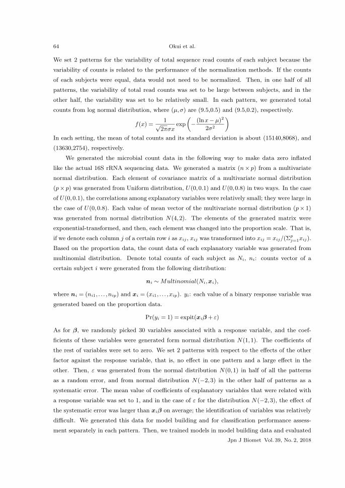
64 Okui et al.

We set 2 patterns for the variability of total sequence read counts of each subject because the

variability of counts is related to the performance of the normalization methods. If the counts

of each subjects were equal, data would not need to be normalized. Then, in one half of all

patterns, the variability of total read counts was set to be large between subjects, and in the

other half, the variability was set to be relatively small. In each pattern, we generated total

counts from log normal distribution, where (µ,σ) are (9.5,0.5) and (9.5,0.2), respectively.

f(x) =1√

2πσxexp

„− (lnx−µ)2

2σ2

«

In each setting, the mean of total counts and its standard deviation is about (15140,8068), and

(13630,2754), respectively.

We generated the microbial count data in the following way to make data zero inflated

like the actual 16S rRNA sequencing data. We generated a matrix (n× p) from a multivariate

normal distribution. Each element of covariance matrix of a multivariate normal distribution

(p× p) was generated from Uniform distribution, U(0,0.1) and U(0,0.8) in two ways. In the case

of U(0,0.1), the correlations among explanatory variables were relatively small; they were large in

the case of U(0,0.8). Each value of mean vector of the multivariate normal distribution (p× 1)

was generated from normal distribution N(4,2). The elements of the generated matrix were

exponential-transformed, and then, each element was changed into the proportion scale. That is,

if we denote each column j of a certain row i as xij , xij was transformed into xij = xij/(Σpj=1xij).

Based on the proportion data, the count data of each explanatory variable was generated from

multinomial distribution. Denote total counts of each subject as Ni, ni: counts vector of a

certain subject i were generated from the following distribution:

ni ∼ Multinomial(Ni,xi),

where ni = (ni1, . . . ,nip) and xi = (xi1, . . . ,xip). yi: each value of a binary response variable was

generated based on the proportion data.

Pr(yi = 1) = expit(xiβ + ε)

As for β, we randomly picked 30 variables associated with a response variable, and the coef-

ficients of these variables were generated form normal distribution N(1,1). The coefficients of

the rest of variables were set to zero. We set 2 patterns with respect to the effects of the other

factor against the response variable, that is, no effect in one pattern and a large effect in the

other. Then, ε was generated from the normal distribution N(0,1) in half of all the patterns

as a random error, and from normal distribution N(−2,3) in the other half of patterns as a

systematic error. The mean value of coefficients of explanatory variables that were related with

a response variable was set to 1, and in the case of ε for the distribution N(−2,3), the effect of

the systematic error was larger than xiβ on average; the identification of variables was relatively

difficult. We generated this data for model building and for classification performance assess-

ment separately in each pattern. Then, we trained models in model building data and evaluated




Table 2. Simulation setting of each pattern

their classification performance in the other data by calculating testing AUC. The coefficients of

classification performance assessment data were set to the same as model building data.

We examined a first experiment for 16 patterns in total. The setting of each pattern is

presented in Table 2. As for the evaluation method of each model, we calculated AUC val-

ues for coincidence between the measure of the degree of association and the true presence or

absence of association with the response variable. Additionally, spearman’s rank correlation co-

efficient between true coefficients and the measure of degree of association were calculated. As

for classification performance, we calculated AUC values for coincidence between the measure

of performance and a response variable. Also, in classification performance evaluation, we cal-

culated AUC values of true model in addition to 19 models for reference. The number of times

that a simulation was conducted was set to 300.

As the second simulation experiment, we confirmed the appropriate sampling times for the

proposed method by varying the sampling times from 10 to 50 by 10.

3.2 Simulation results

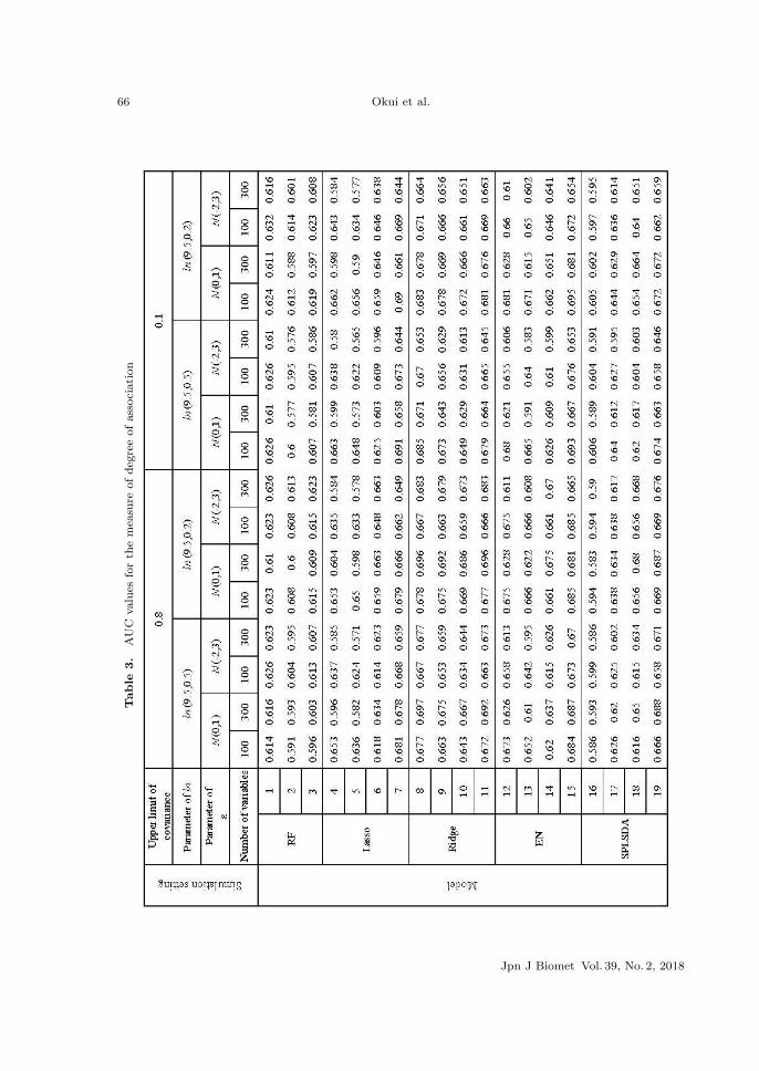
Table 3 shows the result of the AUC values for the coincidence between the measure of the

degree of association and the true presence or absence of association with a response variable,

and Table 4 shows the standard deviations of the AUC values. Among the models that used RF

(1,2,3), the AUC values of model 1, which used proportion data were the highest in all patterns.

But the difference between models 1,2,3 was small in all patterns, and the values are relatively



66 Okui et al.

Table

3.

AU

Cvalu

esfo

rth

em

easu

reofdeg

ree

ofass

oci

ation




Table

4.

Sta

ndard

dev

iation

ofA

UC

valu

esfo

rth

em

easu

reofdeg

ree

ofass

oci

ationw



68 Okui et al.

stable across all patterns. As for Lasso (models 4,5,6,7), the AUC values of the model that used

proportion (model 4) were higher than those of the model that used rarefying (model 5), across

all patterns. This result was also true for Ridge regression and EN. Also, in many cases, the

AUC values of the model that combined proportion with bagging (model 6) were higher than

those of model 4 when the number of subjects was 300, but lower when number of subjects was

100. The AUC values of the model that used the proposed method (model 7) were the highest in

almost all patterns and the values were relatively stable across all patterns. As for Ridge (models

8,9,10,11), the AUC values of the model that combined proportion with bagging (model 10) were

lower than those of the model that used proportion (model 8). The AUC values of model 8 were

the highest in all patterns, and the AUC values of the model that used the proposed method

(model 11) were slightly lower than those of model 8.

As for EN (models 12,13,14,15), the results were almost same as those of Lasso, but the AUC

values of the model that used the proposed method (model 15) were higher than those of Lasso

(model 7) across all patterns. As for SPLSDA (models 16,17,18,19), the AUC values of the model

that used rarefying (model 17) were higher than those for the model that used proportion (model

16) across all patterns. Additionally, the AUC values of the model that combined proportion

with bagging (model 18) were always higher than those of model 16. The AUC values of the

model that used the proposed method (model 19) were the highest in almost all patterns, and

the values were relatively stable across all patterns. Throughout the experiment, in Lasso, Ridge

regression, EN and SPLSDA, the AUC values improved by using the proposed method across

all patterns. On the other hand, this was not the case in RF. If we compare models across

different multivariate data analysis methods, the AUC values of Lasso, Ridge regression, EN

and SPLSDA exceeded those of RF when the proposed method was used. As for the standard

deviations, performance improvement by the proposed method was not apparent evidently.

Table 5 shows the result of spearman’s rank correlation coefficients between the true coef-

ficients and the measure of degree of association, and Table 6 shows the result of the standard

deviations. As for RF, model 3 had the highest correlation coefficients across all patterns. As for

Lasso, Ridge regression, EN and SPLSDA, the correlation coefficients of the models using ensem-

ble learning were higher than those of the models without ensemble learning. As for Lasso, Ridge

regression and EN, the correlation coefficients of the models that used the proposed method were

higher than those of the models that used proportion with bagging across almost all patterns, and

the standard deviations of the correlation coefficients for the proposed method were the lowest

across many patterns. As for SPLSDA, in many patterns, the correlation coefficient values of the

model that used the proposed method were higher than those of the model that used proportion

with bagging when the variance of total counts was large, and lower when the variance of total

counts was small.




Table

5.

Corr

elation

coeffi

cien

tfo

rth

em

easu

reofdeg

ree

ofass

oci

ation



70 Okui et al.

Table

6.

Sta

ndard

dev

iation

ofco

rrel

ation

coeffi

cien

tfo

rth

em

easu

reofdeg

ree

ofass

oci

ation




Table

7.

AU

Cvalu

esfo

rcl

ass

ifica

tion

per

form

ance



72 Okui et al.

Table 7 shows the result of the AUC values for coincidence between the measure of predictive

performance and a response variable, and Table 8 shows the standard deviations. As for RF,

there were no large differences between the models, but the AUC values of model 3 were the

highest across all models. As for Lasso, the AUC values of model 7 were the highest across

many patterns, and the degree of improvement of the AUC values was large when the number

of variables was 300. As for Ridge regression, the AUC values of model 8 and those of model 11

were almost equivalent and the highest across all patterns. As for EN, the AUC values of model

14 evidently dropped, when compared with model 12, when the variance of the total counts were

large or number of variables was 100. The AUC values of model 15 were the highest across all

patterns. As for SPLSDA, the AUC values of model 18 were always higher than those of model

16 when the variance of total counts was small, but this was not the case when the variability

of the total counts was large. The AUC values of model 19 were the highest across all patterns.

Throughout the evaluation of classification performance, the AUC values improved by using the

proposed method in all analysis methods. Also, the standard deviations of the models that used

the proposed method were the lowest in many patterns except for Lasso, where the standard

deviations also improved in model 6 as well as model 7. However, the AUC values and the

standard deviations of the proposed method were inferior to those of the true model.

The second simulation experiment, which evaluated the effect of the sampling times of the

proposed was conducted in the setting of pattern 1 and 2 of Table 2 on behalf of all patterns.

As for the models to evaluate, models 7, 11,15, 19 of Table 1 were used. We did not use RF

model because performance improvement was not confirmed by the proposed method in the first

experiment.

Table 9 shows the result of the second experiment. As for the AUC values and the correlation

coefficients for the measure of the degree of association, the values improved by augmenting

the sampling times when the number of variables was 300, but the degree of improvement was

relatively small in Ridge model. On the other hand, the AUC values for classification performance

did not improve by augmenting the sampling times. When the number of variables was 100, the

two AUC values, the correlation coefficients and their standard deviations did not improve by

augmenting the sampling times.




Table

8.

Sta

ndard

dev

iation

ofA

UC

valu

esfo

rcl

ass

ifica

tion

per

form

ance



74 Okui et al.

Table

9.

The

effec

tofth

esa

mpling

tim

esofth

epro

pose

dm

ethod




4. Real data analysis

We fitted the evaluated models to Japanese gut microbial data. The data was collected at a

medical checkup, which was conducted in the Iwaki district of Hirosaki city in Aomori prefecture

every year. This medical checkup is held as a part of the study for prevention of dementia

and lifestyle-related diseases, and the study’s objective is to develop a preventive method for

multi-factor diseases and promote the health of local residents. The medical checkup’s target is

people older than 20. Gut microbial data began to be collected from 2015. In this study, we

used microbial 16S rRNA sequencing data, which was collected in 2015, and BMI. In 2015, 1148

people participated in the medical checkup, and the number of people whose microbial data and

BMI were collected was 1074.

As for microbiome 16S rRNA sequencing data, DNA was extracted from feces samples, and

amplicon analysis was done by Miseq to V3–V4 regions by techno-suruga labo. Reads sequenced

were grouped into Operational Taxonomic Units (OTUs), and the OTUs were classified microbial

species at the medical institute of University of Tokyo. The classification was done in each

microbial hierarchy, and in this study, we used family and genus as the microbial hierarchy for

data analysis. As the response variable, we used BMI and set 25 as the threshold value and

converted it into a binary variable. We applied each model to the 16S rRNA sequencing data

and compared the results. We used age as an explanatory variable for model building. Table 10

shows the attributes of the subjects and the 16S rRNA sequencing data. The number of families

observed was 110 and the number of genera was 304. The mean of the observed number of families

for each subject was 26.2 and 51.1 for the number of genera, and the number of microbiomes

Table 10. Attributes of subjects and 16S rRNA sequencing data



76 Okui et al.

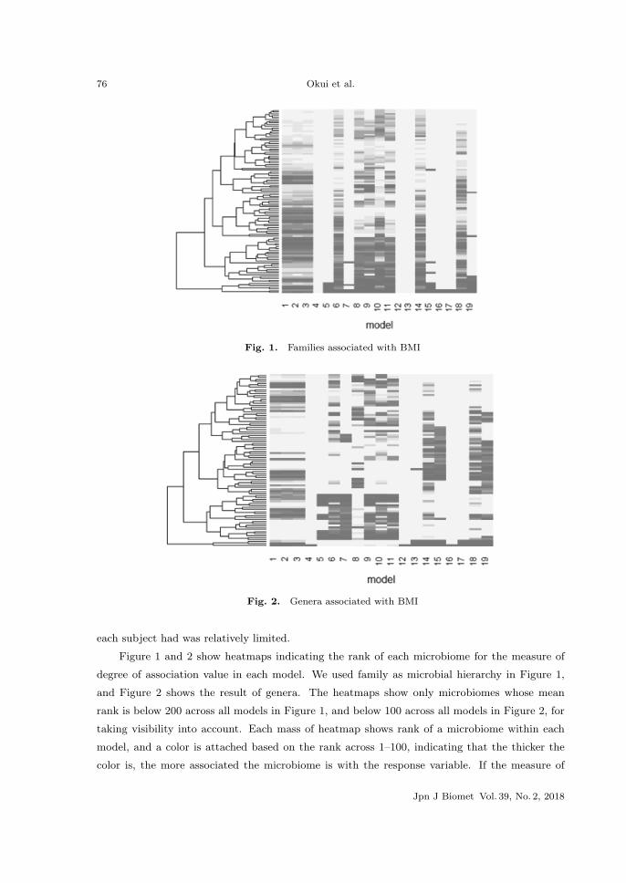
Fig. 1. Families associated with BMI

Fig. 2. Genera associated with BMI

each subject had was relatively limited.

Figure 1 and 2 show heatmaps indicating the rank of each microbiome for the measure of

degree of association value in each model. We used family as microbial hierarchy in Figure 1,

and Figure 2 shows the result of genera. The heatmaps show only microbiomes whose mean

rank is below 200 across all models in Figure 1, and below 100 across all models in Figure 2, for

taking visibility into account. Each mass of heatmap shows rank of a microbiome within each

model, and a color is attached based on the rank across 1–100, indicating that the thicker the

color is, the more associated the microbiome is with the response variable. If the measure of




degree of association of a microbiome was 0, the microbiome’s rank was set to the lowest value.

In Figures 1 and 2, RF models (models 1,2,3) showed similar results. On the other hands, results

of Lasso, Ridge, EN and SPLSDA were different between models across Figure 1–2. As for Lasso,

model 4 scarcely identified microbiomes, and model 6 identified many microbiomes. As for Ridge

regression, all models identified many microbiomes, and the difference between model 9 and 11

was small. As for EN and SPLSDA, models without ensemble learning (models 12,13,16,17)

scarcely identified microbiomes, and models t hat used proportion and bagging (models 14,18)

identified many microbiomes.

5. Discussion

In this study, we focused on normalization methods when multivariate data analysis meth-

ods are used. We then proposed a new association analysis method combining rarefying with

ensemble learning and evaluated its performance in simulation experiments. Although the ef-

ficacy of the ensemble methods was already suggested (Shankar 2015), the significance of this

study is the proposal of a method that incorporates rarefying into the ensemble learning process.

As a result of a simulation experiment, in Lasso, EN and SPLSDA, the proposed method

showed higher performance in terms of AUC values for the measure of degree of association,

correlation coefficient for the measure of the degree of association, and AUC values for classifi-

cation performance, than other methods. As for Ridge regression, the proposed method and the

model that used proportion were almost equivalent in terms of the AUC values for the measure

of degree of association and the AUC values for classification performance. However, the pro-

posed method was superior in terms of the correlation coefficient for the measure of the degree

of association. In contrast to the other methods, the proposed method did not show superior

performance in RF. The cause of this result is unclear, but it is thought that RF is no more

a variable selection method than Ridge regression is, and there is no possibility that the mea-

sure of degree of association of a response-associated variable becomes accidently zero. Then,

the effect of ensemble learning might larger in variable selection methods than other regression

analysis methods. Another possible cause is that RF already uses ensemble learning, and the

bias caused by rarefying did not become zero even when sagging was used. This problem might

be eliminated by augmenting sampling times, but a large improvement would not be achieved

because RF already uses bagging. Furthermore, RF might not be influenced by the pseudo

correlation caused by proportion, unlike ordinary regression models, because the results were

relatively stable across patterns. Results of the simulation experiment indicate that when RF is

used, the normalization method does not markedly influence the result. Lasso, Ridge regression,

EN and SPLSDA are ordinary regression models, each of which learns the model without en-

semble learning in itself, and the correlation coefficient values rose by using ensemble learning in

these models. Additionally, in the real data analysis, microbiomes are rarely identified in many

models without ensemble learning (models 4,12,13,16,17); ensemble learning is thought to be



78 Okui et al.

important for evaluating the effect of variables. However, taking into account the result of AUC

values for the measure of the degree of association, the coefficient estimates of variables which

were not related to a response variable were overestimated by pseudo-correlation in models that

combined proportion with bagging. Results of the real data analysis show that models combining

proportion with bagging (models 6,10,14,18) identified many microbiomes, but the measure of

the degree of association of many microbiomes might be overestimated.

As for classification performance, in Lasso, Ridge regression, SPLSDA and EN, when the

variability of the total counts was large and the number of variables was 100, AUC values dropped

by using the models combining proportion with bagging, compared with the models that used

proportion. When the variability of total counts was large, the effect of pseudo correlation by

proportion data augmenting and the generalizability of the coefficient estimates of the models that

used proportion worsened. As a result, the models using proportion with bagging overestimated

the coefficient estimates more than the models that used proportion only, evidenced by the result

of the AUC value and correlation coefficient for the measure of association. Though the AUC

values for the measure of the degree of association and the correlation coefficients for the measure

of the degree of association remained low across all models, the cause for it is considered to be

the simulation setting wherein variables whose values were almost all zero became the associated

variables for a response variable in many cases. As a result, the difference between the proposed

method and the true model was large in terms of the AUC values for classification performance.

From these results, in Lasso, Ridge regression, SPLSDA and EN, one can identify variables

associated with a response variable more accurately by using the proposed method. On the other

hand, RF’s performance was worse than models with the proposed method (models 7,11,15,19)

across all patterns. RF is one of the most commonly used analysis methods for 16S rRNA se-

quencing data; it is often used with rarefying. But from this experiment, it was suggested that

other regression models with the proposed method would identify response-associated explana-

tory variables more accurately. As for proportion data, the performance of the models with

proportion was superior to the models with rarefying when ensemble learning was not used in

many cases. Proportion data is generally avoided because it is compositional data, but it was

suggested that when the number of variables become larger, the problem of proportion data

become smaller. We did not examine cases of 1000 or more variables for computational burden;

proportion data might have no problems if data of microbiome hierarchy, such as species was

used. As for the sampling times of the proposed method, 10 times were sufficient when the

number of variables was 100. On the other hand, when the number of variables was 300, the

performance improved by augmenting the sampling times, especially in terms of the correlation

coefficient for the measure of degree of association. We can identify variables associated with a

response variable more accurately by augmenting the sampling times when the number of vari-

ables is large, but difference between 10 times and 50 times was relatively small. It depends on




data, but, if the computational burden is large, about 10 times might be sufficient.

In identifying microbiomes associated with a response variable, the shortcoming of ensemble

learning is that the interpretation of results from the analysis becomes difficult. When we use

the proposed method, there are cases where we cannot judge whether a microbiome is associated

with the response variable based on the rank of coefficient estimates. If we want to select

variables, one proposal is that we adopt variables based on the rank of coefficient estimates,

until a variable where classification error in other data is minimized. Other association methods

such as differential abundance analysis or ordinary variable selection models can select variables

easily, but their selection is not always accurate and they cannot evaluate the effect of variables

associated with the response variable like ensemble-learning methods. If the association with

the response variable is relatively limited like the real data analysis in this study, the identified

variables do not augment considerably even when the proposed method was used in Lasso, EN

and SPLSDA (models 7,15,19). On the other hand, if we use Ridge regression with the proposed

method (model 11), many variables are identified (Figure 1,2) because the coefficient estimates

are not forced to become zero in Ridge regression. Then, Ridge regression is inferior to the other

methods in terms of ease of interpretation of analysis results. If we want to build a classification

model with a response variable rather than identify variables associated with a response variable,

the proposed method is useful for the four analysis methods including Ridge regression.

A limitation of this study is that we examined only 5 major association analysis methods;

other methods should also be examined. Other methods, for example, support vector machine

and nearest shrunken centroids (Knights 2011) are used, but if the method does not include

ensemble learning in the learning process, the ability in identification of response-associated

microbiomes would improve by using the proposed method. The degree of improvement when

using the proposed depends on the analysis method. Another limitation was that we did not

examine the ordinary approaches for compositional data, that is, log-ratio transformation and

the method which uses one variable as reference. These methods are used as the normalization

methods for Lasso, EN and SPLSDA. As shown in Table 10, a variety of microbiomes which

one subject has are limited, and there are a lot of zero values in the 16S rRNA sequencing

data. In real data analysis, we could not use log-ratio transformation even after imputing zero

values with small values, because the computation involved multiplying many tiny values and

estimation could not be done. Omitting tiny microbiomes in advance from data analysis may

solve this problem, but 16S rRNA sequencing data are collections of such tiny microbiomes.

Then, omitting tiny microbiomes may make data analysis meaningless. By using the proposed

method, one can identify response-associated microbiomes without omitting microbiomes. The

ordinary approaches for compositional data were not developed for 16S rRNA sequencing data,

and if we use data with a large variety of microbiomes, like genus or species, these methods

cannot be used properly.



80 Okui et al.

As mentioned in the introduction, although proportion data are considered to be a problem,

simulation experiments for multivariate data analysis methods have not yet been tried, and

methods like rarefying or log-ratio transformation are used arbitrarily. As the simulation results

suggest, performance of analysis methods varies depending on the normalization methods. The

simulation patterns we examined were limited in that parameters like number of subjects, total

read counts and their variability are more diverse in reality. As for total read counts, the values

vary between a few thousand and several hundred million. Then, broader simulation experiments

for normalization methods should be performed in the future.

6. Conclusion

We proposed a new association method that combines rarefying with ensemble learning

and examined its performance. As a result, it was suggested that if we use ordinary regression

models, we can identify microbiomes associated with a response variable and classify the response

variable more accurately using the proposed method.

Acknowledgements

This research is partially supported by the Center of Innovation Program from Japan Science

and Technology Agency, JST. Additionally, we would like to thank for the two referees for their

thorough review of the manuscript and appropriate comments.

REFERENCES

Aitchison J (1982). The statistical analysis of compositional data. Journal of the royal statistical

society , 44: 139–177.

Acharjee A, Finkers R, Visser RGF, Maliepaard C (2013). Comparison of regularized regression

methods for omics data. Metabolomics; 3: 3.

Breiman L, Friedman JH, Olshen RA, Stone CJ (1984). Classification and Regression Trees.

Chapman & Hall (Wadsworth, Inc.): New York.

Breiman L (1996). Bagging predictors. Machine learning , 24: 123–140.

Breiman L (2001). Random forests. Machine Learning , 45: 5–32.

Breiman L, Cutler A, Liaw A, Wiener M (2015). package ‘randomForest’ Breiman and Cut-

ler’s Random Forests for classification and regression. https://cran.r-project.org/web/

packages/randomForest/randomForest.pdf.

Buhlmann P, Hothorn T (2007). Boosting algorithms: regularization, prediction and model fit-

ting. Statistical science, 22, 477–505.

Cao KA Le, Costello ME, Lakis VA, Bartolo F, Chua XY (2016). MixMC: A multivariate sta-

tistical framework to gain insight into microbial communities. PloS One, 11: 8.




Cao KA Le, Rohart F, Gonzalez I, Dejean S, Gautier B, Bartolo F (2017). package ‘mixOmics’

omics data integration projects., https://cran.r-project.org/web/packages/mixOmics/

mixOmics.pdf.

Cao KA Le, Boitard S, Besse P (2011). Sparse PLS discriminant analysis: biologically relevant

feature selection and graphical displays for multiclass problems. BMC Bioinformatics, 12:

253.

Chen W, Liu F, Ling Z, Tong X, Xiang C (2012). Human intestinal lumen and mucosa-associated

microbiota in patients with colorectal cancer. PLoS One, 7.

Cho S, Kim K, Kim YJ, Lee JK, Cho YS, Lee JY, Han BG, Kim H, Ott J, Park T (2010). Joint

identification of multiple genetic variants via elastic-net variable selection in a genome-wide

association analysis. Annals of human genetics, 74: 416–428.

Chua LL, Rajasuriar R, Azanan MS, Abdullah NK, Tang MS, Lee SC, Woo YL, Lim YAL,

Ariffin H, Loke P (2017). Reduced microbial diversity in adult survivors of childhood acute

lymphoblastic leukemia and microbial associations with increased immune activation. Mi-

crobiome, 5: 35.

Chun H, Keles S (2010). Sparse partial least squares regression for simultaneous dimension

reduction and variable selection. Journal of the Royal statistical society , 72: 2–25.

Chung D, Keles S (2010). Sparse partial least squares classification for high dimensional data.

Statistical applications in genetics and molecular biology , 9: 1.

Chung D, Chun H, Keles S (2015). package ‘spls’ sparse partial least squares(SPLS) regression

and classification. https://cran.r-project.org/web/packages/spls/spls.pdf.

Determan Jr. CE (2015). Optimal algorithm for metabolomics classification and feature selection

varies by dataset. International journal of biology , 7: 1.

Friedman J, Hastie T, Tibshirani R (2010). Regularization paths for generalized linear models

via coordinate descent. Journal of statistical software, 33: 1.

Friedman J, Hastie T, Simon N, Qjan J, Tibshirani R (2017). package ‘glmnet’ lasso and elastic-

net regularlized generalized linear models, https://cran.r-project.org/web/packages/

glmnet/glmnet.pdf.

Garcia TP, Muller S, Carroll RJ, Walzem RL (2014). Identification of important regressor groups,

subgroups and individuals via regularization methods: application to gut microbiome data.

Bioinformatics, 30: 831–837.

Gregory B, Reid G (2016). Compositional analysis: a valid approach to analyze microbiome

high-throughput sequencing data. NRC research press, 62: 692–703.

Halfvarson J, Brislawn CJ, Lamendella R, Vazquez-Baeza Y, Walters WA, Bramer LM, D’Amato

M, Bonfiglio F McDonald D, Gonzalez A, McClure EE, Dunklebarger MF, Kinght R &



82 Okui et al.

Jansson JK (2017). Dynamics of the human gut microbiome in inflammatory bowel disease.

Nature microbiology , 2.

Hastie T, Tibshirani R, Friedman J (2009). The Elements of Statistical Learning; Data Mining,

Inference and Prediction 2ed. Springer: New York.

Hoerl AE, Kennard RW (1970). Ridge regression: Biased estimation for nonorthogonal problems.

Technometrics, 12: 55–67.

Jacobs JP, Goudarzi M, Singh N, Tong M, Mchardy IH, Ruegger P, Asadourian M, Moon BH,

Ayson A, Bomeman J, McGoyern DP, Fornace AJ Jr, Braun J, Dubinsky M (2016). A

disease-associated microbial and metabolomics state in relatives of pediatric inflammatory

bowel disease patients. Cellular and molecular gastroenterology , 2: 750–766.

Jiang M, Wang C, Zhang Y, Feng Y, Wang Y, Zhu Y (2014). Sparse partial least squares

discriminant analysis for differential geographical origins of Salvia miltiorrhiza by 1H-NMR-

bases metabolomics. Phytochemical analytics, 25: 50–58.

Kim M, Lee KH, Yoon SW, Kim BS, Chun J, Yi H (2013). Analytical tools and databases for

metagenomics in the next-generation sequencing era. Genomics & Informatics, 11: 102–113.

Knights D, Costello EK, Knight R (2011). Supervised classification of human microbiota. FFMS

microbiology reviews, 35: 342–359.

Labus JS, Hollister EB, Jacobs J, Kirbach K, Owzguen N, Gupta A, Acosta J, Luna RA, Aagaard

K, Versalovic J, Savidge T, Hsiao E, Tillisch K, Mayer EA (2017). Differences in gut microbial

composition correlate with regional brain volumes in irritable bowel syndrome. Microbiome,

5: 49.

Lee SC, Tang MS, Lim YAL, Choy SH, Kurtz ZD, Cox LM, Gundra UM, Cho I, Bonneau R,

Blaser MJ, Chua KH, Loke PNG (2014). Helminth colonization is associated with increased

diversity of the gut microbiota. PloS neglected tropical diseases, 8: 5.

Lin W, Shi P, Feng R, Li H (2014). Variable selection in regression with compositional covariates.

Biometrika, 101: 785–797.

Lu D, Weljie A, de Leon AR, McConnell Y, Bathe OF, Kopciuk K (2017). Performance of variable

selection methods using stability-based selection. BMC research notes, 10: 143.

Mach N, Berri M, Estelle J, Levene F, Lemonnier G, Denis C, Leplat JJ, Chevaleyre C, Billon

Y, Dore J, Rogel-Gaillard C, Lepage P (2015). Early-life establishment of the sqine gut

microbiome and impact on host phenotypes. Environmental microbiology reports, 7: 554–

569,

Mahana D, Trent CM, Kurtz ZD, Bokulich NA, Battaglia T, Chung J, Muller CL, Li H, Bonneau

RA, Blaser MJ (2016). Antibiotic perturbation of the murine gut microbiome enhances




the adiposity, insulin resistance, and liver disease associated with high-fat diet. Genome

Medicine, 8: 48.

Mandel S, Treuren WV, White RA, Eggesbo M, Kinght R, Peddada SD (2015). Analysis of

composition of microbiomes: a novel method for studying microbial composition. Microbial

ecology in health and disease, 26: 1.

McMurdie PJ, Holmes S (2014). Waste not, want not: why rarefying microbiome data is inad-

missible. PloS One computational biology , 10: 4.

Mevik BH, Wehrens R (2016). Introduction to the pls Package. https://cran.r-project.org/

web/packages/pls/vignettes/pls-manual.pdf.

Michaelson JJ, Alberts R, Schughart K, Beyer A (2010). Data-driven assessment of eQTL map-

ping methods. BMC bioinformatics, 11: 502.

Naseribafrouei A, Hestad K, Avershina E, Sekelja M, Linlokken A, Wilson R, Rudi K (2014).

Correlation between the human fecal microbiota and depression. Neurogastroenterology , 26:

1155–1162.

Oulas A, Pavloudi C, Polymenakou P, Pavlopoulas GA, Papanikolaou N, Kotoulas G et al. (2015).

Metagenomics: tools and insights for analyzing next-generation sequencing data derived from

biodiversity studies. Bioinformatics and biology insights, 9: 75–88.

Paulson JN, Stine OC, Bravo HC, Pop M (2013). Differential abundance analysis for microbial

marker-gene surveys. Nature methods, 10.

Rapaport F, Khanin R, Liang Y, Pirun M, Krek A, Zumbo P, Mson CE, Socci ND, Betel D

(2013). Comprehensive evaluation of differential gene expression analysis methods for RNA-

seq data. Genome Biology, 14.

R Core Team (2017). R: a language and environment for statistical computing. R Foundation

for Statistical Computing. Vienna, Austria URL http://www.R-project.org/.

Robin X, Turck N, Hainard A, Tiberti N, Lisacek F, Sanchez JC, Muller M, Siegest S (2017).

package ‘pROC’ display and analyze ROC curves. https://cran.r-project.org/web/

packages/pROC/pROC.pdf.

Robinson MD, Oshlack A (2010). A scaling normalization method for differential expression

analysis of RNA-seq data. Genome Biology , 11.

Rohart F, Gautier B, Singh A, Cao KL (2017). mixOmics: an R package for ’omics feature

selection and multiple data integration. In draft https://biorxiv.org/content/biorxiv/

early/2017/08/108597.full.pdf.

Rush ST, Lee CH, Mio W, Kim PT (2016). The phylogenetic lasso and the microbiome. https:

//arxiv.org/pdf/1607.08877.pdf.



84 Okui et al.

Schubert AM, Rogers MAM, Ring C, Mogle J, Petrosino JP, Young VB, Aronoff DM, Schloss

PD (2014). Microbiome data distinguish patients with Clostridium difficile infection and

non-C. difficile-associated diarrhea from healthy controls. mBio, 5.

Shankar J, Szpalowski S, Solis NV, Mounaud S, Liu H, Losada L, Nierman WC, Filler SG (2015).

A systematic evaluation of high-dimensional, ensemble-based regression for exploring large

model spaces in microbiome analyses. BMC bioinformatics, 16: 31.

Shimokawa T, SugimotoT, Goto M (2013). Tree structure approach: Learning data science by R

9. Kyoritsu syuppann.

Statnikov A, Henaff M (2013). A comprehensive evaluation of multicategory classification meth-

ods for microbiome data. Microbiome, 1: 11.

Tap J, Derrien M, Tornblom H, Brazeilles R, Cools-Portier S, Dore J, Storsrud S, Neve B-L,

Ohman L, Simren M: Identification of an intestinal microbiota signature associated with

severity of irritable bowel syndrome. Gastroenterology 2017, 152: 111–123.

Tibshirani R (1996). Regression shrinkage and selection via the lasso. Journal of the royal sta-

tistical society B(Methodology), 58: 267–288.

Tsilimigras MCB, Fodor AA (2016). Compositional data analysis of the microbiome: fundamen-

tals, tools, and challenges. Annals of epidemiology , 26: 330–335.

Warnes GR, Bolker B, Bonebakker L, Gentleman R, Liaw WHA, Lumley T, Maechler M, Magnus-

son A, Moeller S, Schwantz M, Venebles B (2016). Packages ‘gplots’ various R programming

tools for plotting data. https://cran.r-project.org/web/packages/gplots/gplots.pdf.

Weiss S, Xu ZZ, Peddada S, Amir A, Bittinger K, Gonzalez A, Lozupone C et al. (2017). Nor-

malization and microbial differential abundance strategies depend upon data characteristics.

Microbiome 2017, 5: 27.

Wu N, Yang X, Zhang R, Li J, Xiao X, Hu Y, Chen Y, Yang F et al. (2013). Dysbiosis signature

of fecal microbiota in colorectal cancer patients. Microbiome Ecology , 66: 462–470.

Yang P, Yang HY, Bing BZ, Albert YZ (2010). A review of ensemble methods in bioinformatics.

Current bioinformatics, 5: 296–308.

Yatsunenko T, Rey FE, Manary MJ, Trehan I, Dominguez-Bello MG, Contreras M et al. (2012).

Human gut microbiome viewed across age and geography. Nature, 486: 222–227.


Original Article - JST

Documents

Transcript of Original Article - JST