Orientation Distribution Function (ODF)

Limitation of pole figures:

3 D orientation distribution 2 D projection loss in information

Poor resolution ambiguity in orientation determination

Incompletely determined limitation in experimental procedure

Three dimensional Orientation Distribution Function

Analysis of several pole figures is required.

A pole which is defined by a direction y, e.g. (, ) in a given 2 D pole figure Ph(y) corresponds to a region in the 3 D ODF which contains all possible rotations with angle about this direction y in the pole figure.

That is,

Assumption:

•Both the measured pole figure and the resulting ODF can be fittedby a series expansion with suitable mathematical functions

Spherical Harmonic functions

Harmonic method, or Series expansion method

Spherical Harmonic functions

can be calculated for all the orientations `g´- usually stored in libraries

Therefore, ODF f(g) can be completely described by the series expansion coefficients `c´

where Fnl are series expansion coefficients, and Kn

l(y) are the spherical harmonic function

Usually several pole figures Ph are required to calculate the ODF.Lower the symmetry of crystal structure, higher number of pole figures are required.

For cubic, 3-4 pole figures are desirableFor hexagonal, 6 pole figures are requiredFor orthorhombic, 7 pole figures are a must.

14

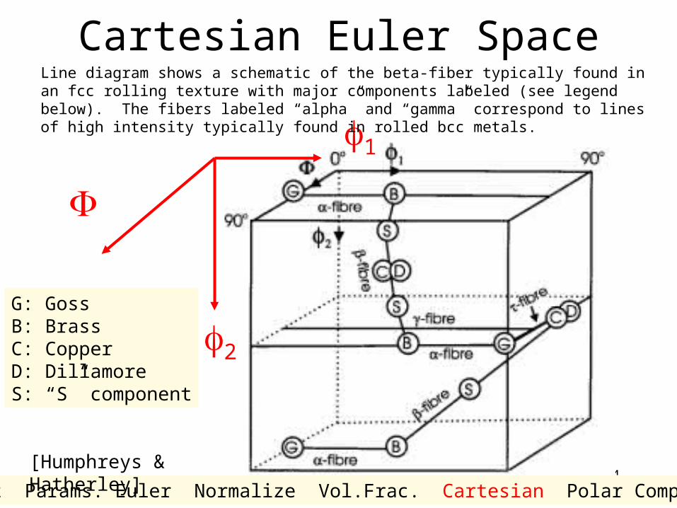
Cartesian Euler Space

1

2

Concept Params. Euler Normalize Vol.Frac. Cartesian Polar Components

[Humphreys & Hatherley]

Line diagram shows a schematic of the beta-fiber typically found in an fcc rolling texture with major components labeled (see legend below). The fibers labeled “alpha” and “gamma” correspond to lines of high intensity typically found in rolled bcc metals.

G: GossB: BrassC: CopperD: DillamoreS: “S” component

15

OD Sections2 = 0°

2 = 5° 2 = 15°2 = 10°

1

2

Concept Params. Euler Normalize Vol.Frac. Cartesian Polar Components

Sections are drawn as contour maps, one per value of 2 (0, 5, 10 … 90°).

Example of copper rolled to 90% reduction in thickness ( ~ 2.5)

BB

SS

CCDD

GG

[Humphreys & Hatherley]

[Bunge]

16

Example of OD in Bunge Euler Space

• OD is represented by aseries of sections, i.e. one(square) box per section.• Each section shows thevariation of the OD intensityfor a fixed value of the thirdangle.• Contour plots interpolatebetween discrete points.• High intensities mean that the corresponding orientation is common (occurs frequently).

1

Section at 15°

Concept Params. Euler Normalize Vol.Frac. Cartesian Polar Components

[Bunge]

17

Example of Example of OD in Bunge OD in Bunge Euler Space, Euler Space,

contd.contd.This OD shows the textureof a cold rolled copper sheet.Most of the intensity isconcentrated along a fiber.Think of “connect the dots!”

The technical name for this is the beta fiber.

Concept Params. Euler Normalize Vol.Frac. Cartesian Polar Components

[Bunge]

18

Numerical ⇄

Graphical

CUR80-2 6/13/88 COMPUTED BY WIMV 6-MAR-89 CODK 5.0 90.0 5.0 90.0 1 1 1 2 3 100 phi= 45.0 3 3 3 3 4 9 14 43 82 99 82 43 14 9 4 3 3 3 3 2 3 3 4 7 11 15 32 56 58 51 47 29 13 6 5 4 3 4 3 3 3 3 4 5 10 33 43 63 82 73 50 32 18 13 9 9 12 3 4 7 7 9 6 18 15 51 99 143 161 128 102 77 59 52 42 42 4 4 5 6 3 9 6 14 23 39 72 117 159 167 149 158 166 177 191 2 1 2 3 4 4 7 7 10 20 51 108 156 191 258 387 567 760 835 1 1 2 2 2 3 3 3 3 8 22 48 104 184 299 551 9991526 1765 1 1 1 1 2 1 1 2 4 6 15 26 49 87 148 248 505 837 930 1 1 2 1 1 1 2 1 2 4 7 13 23 34 42 56 80 89 82 1 1 1 2 2 2 3 3 3 4 9 12 15 19 28 29 33 38 36 1 2 2 1 1 1 1 1 1 2 2 2 2 2 2 3 3 3 4 2 2 2 2 1 1 1 1 1 2 2 2 2 2 2 2 1 1 1 5 4 4 4 4 3 3 3 3 2 2 2 1 1 2 1 1 1 1 9 11 9 10 13 15 9 9 9 6 6 6 6 4 4 4 3 3 3 9 12 13 13 18 18 14 16 15 15 16 11 8 7 7 5 4 3 2 25 28 33 31 33 35 34 37 43 52 63 74 55 22 10 14 10 7 7 14 13 15 16 17 18 20 24 36 57 88 113 102 66 36 28 23 21 18 5 7 9 9 14 24 31 46 94 200 342 418 377 285 205 158 148 138 138 13 13 13 14 20 31 50 99 201 505 980132013781155 835 646 480 382 346

1

2 = 45°

Example of asingle section

Concept Params. Euler Normalize Vol.Frac. Cartesian Polar Components

[Bunge]

19

(Partial) Fibers in fcc Rolling Textures

1

2

C = Copper

B = Brass

Concept Params. Euler Normalize Vol.Frac. Cartesian Polar Components

[Bunge]

[Humphreys & Hatherley]

20

OD ⇄ Pole Figure

1

B = Brass C = Copper

2 = 45°

Note that any given component that is represented as a point in orientation space occurs in multiple locations in each pole figure.

Concept Params. Euler Normalize Vol.Frac. Cartesian Polar Components

[Kocks, Tomé, Wenk]

<100>

{001}

<100>

{011}

21

Rotation 1 (φ1): rotate sample axes about ND

Rotation 2 (Φ): rotate sample axes about rotated RD

Rotation 3 (φ2): rotate sample axes about rotated ND

aComponent Euler Angles (°)

Cube (0, 0, 0)

Goss (0, 45, 0)

Brass (35, 45, 0)

Copper (90, 45, 45)

010

001

Texture Components vs. Orientation Space

Φ φ1

φ2

Cube {100}<001> (0, 0, 0)Goss {110}<001> (0, 45, 0)

Brass {110}<-112> (35, 45, 0)

Orientation Space

Slide from Lin Hu [2011]

22

Φ φ1

φ2

Cube {100}<001> (0, 0, 0)Goss {110}<001> (0, 45, 0)

Brass {110}<-112> (35, 45, 0)

ODF gives the density of grains having a particular orientation.ODF gives the density of grains having a particular orientation.

ODF: 3D vs. sections

ODFOrientation Distribution Function f (g)

ODFOrientation Distribution Function f (g)

g = {φ1, Φ, φ2}

Slide from Lin Hu [2011]

23

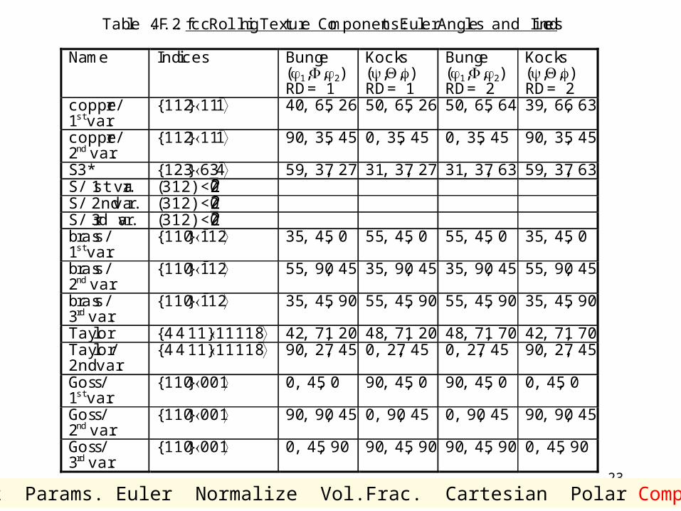
Table 4.F.2. fcc Rolling Texture Components: Euler Angles and Indices

Name Indices Bunge(1,,2)RD= 1

Kocks(,,)RD= 1

Bunge(1,,2)RD= 2

Kocks(,,)RD= 2

copper/1st var.

{112}111̄ 40, 65, 26 50, 65, 26 50, 65, 64 39, 66, 63

copper/2nd var.

{112}111̄ 90, 35, 45 0, 35, 45 0, 35, 45 90, 35, 45

S3* {123}634̄ 59, 37, 27 31, 37, 27 31, 37, 63 59, 37, 63S/ 1st var. (312)<0 2 1> 32, 58, 18 58, 58, 18 26, 37, 27 64, 37, 27S/ 2nd var. (312)<0 2 1> 48, 75, 34 42, 75,34 42, 75, 56 48, 75, 56S/ 3rd var. (312)<0 2 1> 64, 37, 63 26, 37, 63 58, 58, 72 32, 58, 72brass/1st var.

{110}1̄12 35, 45, 0 55, 45, 0 55, 45, 0 35, 45, 0

brass/2nd var.

{110}1̄12 55, 90, 45 35, 90, 45 35, 90, 45 55, 90, 45

brass/3rd var.

{110}1̄12 35, 45, 90 55, 45, 90 55, 45, 90 35, 45, 90

Taylor {4 4 11}11 11 8̄ 42, 71, 20 48, 71, 20 48, 71, 70 42, 71, 70Taylor/2nd var.

{4 4 11}11 11 8̄ 90, 27, 45 0, 27, 45 0, 27, 45 90, 27, 45

Goss/1st var.

{110}001 0, 45, 0 90, 45, 0 90, 45, 0 0, 45, 0

Goss/2nd var.

{110}001 90, 90, 45 0, 90, 45 0, 90, 45 90, 90, 45

Goss/3rd var.

{110}001 0, 45, 90 90, 45, 90 90, 45, 90 0, 45, 90

Concept Params. Euler Normalize Vol.Frac. Cartesian Polar Components

24

Miller Index

Map in Euler Space

Bunge, p.23 et seq.

Concept Params. Euler Normalize Vol.Frac. Cartesian Polar Components

25

2 = 45° section,Bungeangles

Goss

Copper

BrassConcept Params. Euler Normalize Vol.Frac. Cartesian Polar Components

Gamma fiber

Alp

ha fi

ber

26

3D Viewsa) Brass b) Copper c) S d) Goss e) Cube f) combined texture 1: {35, 45, 90}, brass, 2: {55, 90, 45}, brass3: {90, 35, 45}, copper, 4: {39, 66, 27}, copper5: {59, 37, 63}, S, 6: {27, 58, 18}, S, 7: {53, 75, 34}, S 8: {90, 90, 45}, Goss 9: {0, 0, 0}, cube 10: {45, 0, 0}, rotated cube