Orientation Angle Estimation from PolSAR Data using aStochastic Distance

Avik Bhattacharya1, Arnab Muhuri1, Shaunak De1, Alejandro C. Frery2

1Centre of Studies in Resources Engineering, IIT-Bombay

2LaCCAN

International Geoscience and Remote Sensing Symposium (IGARSS 2014)Quebec, Canada

Introduction

I The angle of rotation of any object about the line of sight (LOS) is known as thepolarization orientation angle (OA) θ0.

I OA is found to be non zero for undulating terrains and man-made targets orientedaway from the radar LOS. This effect is more pronounced at lower frequencies (eg.L- and P- bands).

I OA shift is not only induced by azimuthal slope but also by range slope.

Introduction

I The OA shift increases the cross-polarization (HV) intensityand subsequently the covariance or the coherency matrixbecomes reflection asymmetric.

I Compensating this OA prior to any model-baseddecomposition technique for geophysical parameterestimation or classification is crucial.

I In this paper we propose to estimate the OA (θ0) bymaximizing the Hellinger distance between the un-rotatedand rotated diagonal elements of the coherency matrix.

Stochastic Distance

I The stochastic distance (divergence) is any symmetric, non-negative function oftwo probability measures.

I For two random matrices X and Y having densities fX (Z′, θ1) and fY (Z′, θ2)respectively, the (h, φ) divergence between fX and fY is defined by

I Where A is the support matrix, φ : (0,∞)→ [0,∞) is a convex function andh : (0,∞)→ [0,∞) is a strictly increasing function with h(0) = 0

Stochastic Distance

dhφ(X,Y) =

Dhφ(X,Y)+Dh

φ(Y,X)

2

dhφ : A×A → R are distances over A

The Hellinger distance is defined by:dH(X,Y) = 1−

∫ √fXfY

Methodology

The effect of the OA (θ) obtained from Lee and Ainsworth (2011) as on the threediagonal elements of the coherency matrix states that:

1. T11 = |HH + VV |2 /2 is roll invariant for any θ

2. T22 = |HH − VV |2 /2 always increases or remains the same after the OAcompensation

3. T33 = 2 |HV |2 always decreases or remains the same after OA compensation.

OA (θ) obtained from Lee and Ainsworth (2011)

θ =1

4tan−1

(−2Re(T23)

T33 − T22

)(1)

The orientation angle θ is in the range [−π8 ,

π8 ]

J.-S. Lee and T. Ainsworth. The effect of orientation angle compensation on coherency matrix and polarimetric target decompositions. Geoscienceand Remote Sensing, IEEE Transactions on, 49(1):53–64, Jan 2011. ISSN 0196-2892. doi: 10.1109/TGRS.2010.2048333.

J.-S. Lee, D. Schuler, and T. Ainsworth. Polarimetric sar data compensation for terrain azimuth slope variation. Geoscience and Remote Sensing,IEEE Transactions on, 38(5):2153–2163, Sep 2000. ISSN 0196-2892. doi: 10.1109/36.868874.

Methodology

I In PolSAR data analysis, z is often assumed to obey multivariate complexGaussian distribution f (z ; Σ) with zero mean (2),

f (z ; Σ) =1

πp |Σ|exp(−z∗TΣ−1z) (2)

I The p × p Hermitian positive definite matrix A = nZ follows a complex Wishartdistribution given by (3)

f (A) =|A|L−p exp[−Tr(Σ−1A)]

Γp(L) |Σ|L(3)

Γp(L) = πp(p−1)

2

p∏i=1

Γ(L− i + 1) =

∫A

|A|(L−p) exp[Tr(A)] dA (4)

Methodology

I The Hellinger distance between two central complex Wishart distribution forΣ1 6= Σ2 (different covariance matrices) and L1 = L2 = L (same number of looks)is given by (5),

DH = 1−∫ √

f1(A)f2(A) = 1− |Σ1|L/2 |Σ2|L/2∣∣∣Σ12 + Σ2

2

∣∣∣L (5)

Methodology

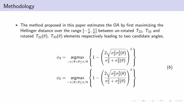
I The method proposed in this paper estimates the OA by first maximizing theHellinger distance over the range [−π

4 ,π4 ] between un-rotated T22, T33 and

rotated T22(θ), T33(θ) elements respectively leading to two candidate angles,

φ3 = argmax−π/4<θ≤π/4

1−

2√σ2

3σ23(θ)

σ23 + σ2

3(θ)

L

φ2 = argmax−π/4<θ≤π/4

1−

2√σ2

2σ22(θ)

σ22 + σ2

2(θ)

L

(6)

Methodology

Two maxima are found at φ = φ{3,2} and φ = φ{3,2} ± π/4, and the OA is chosen suchthat the Hellinger distance (DHφ3) corresponding to σ2

3 is greater than the Hellingerdistance (DHφ2) corresponding to σ2

2 either at φ = φ{3,2} or at φ = φ{3,2} ± π/4.

Figure: Estimated angle from Hellinger distance (Red: T33, Blue: T22)

Methodology

I This condition exactly corresponds to the case where the cross-polarized (HV )component is minimized

I The other peak corresponds to the situation where the HV component isincorrectly maximized.

I The OA (θ0) is obtained in the range [−π8 ,

π8 ] by

θ0 =

φ+ π/4, if φ < −π/8

φ− π/4, if φ > π/8

φ, otherwise

(7)

Results

Figure: (a) Pauli RGB (R=< |SHH − SVV | > , G=< 2|SHV | >, B=< |SHH + SVV | >), (b)Estimated OA angle from Lee et al. (2000), (c) Estimated OA angle from the proposed method

Match with Lee et al. (2000)’s Method

I The results from the proposed method and the one described in Lee et al. (2000)show a high degree of similarity

I Difference between the two results is almost zero, as shown:

Theta

Figure: Histogram of difference in θ0 computed from the proposed and that describedin Lee et al. (2000)

Results

Figure: Comparison of OA estimated from Lee et al. (2000) and the proposed method (Blue:Lee et. al, Red: Proposed method)

Results

Figure: Real orientation angle (a) real orientation angle obtained by the proposed method, (b)real orientation angle obtained by the method of (Lee and Ainsworth, 2011), (c) comparison ofthe estimated orientation angle for the given transect, (d) histogram of the difference inorientation angle computed for the entire scene by the two methods.

Summary

I The proposed method is tested on an AIRSAR San-Francisco L-band image withsome built-up areas oriented from the LOS (A and B)

I The comparison of OA estimated from Lee et al. (2000) and the proposed methodalong the horizontal profile (Red line) in is shown.

I As it can be seen the proposed OA estimation exactly matches the OA estimatedfrom Lee et al. (2000).

I The average OA estimated over region A is −4◦ and the average OA over regionB is 6◦.

I The region C is perpendicular to the LOS and hence the OA estimated is ∼ 0.The proposed method gives an insight into the behavior of the T22 and T33

elements with the change in the orientation angle.

I The usefulness of the Hellinger distance as a polarimetric descriptor will be furtherinvestigated.