MATH REVIEW 2019

August 30, 2019 Professor: Alan G. Isaac

Location: Kreeger 100 (or possibly MGC 247 as a backup) Here are the

places and times:

M 26 Aug: 1pm-4pm

W 28 Aug: 9am-12pm

Th29 Aug: 1pm-4pm

Organization

During the scheduled hours I will lecture. You should allocate as much

as possible of the rest of the day for group reading and problem solving. (I

strongly encourage working in groups.) Ideally, evenings will be for individual

reading in preparation for the next lecture.

1

Day 1

Introduction to Mathematica

Functions

Lists as Vectors

Lists as Matrices

Comparative Statics with Linear Models

Recommended Reading: Klein ch.1; Hoy ch. 1;

Klein ch.4,5;

Independent Review: Do end of chapter problems.

Day 2

Differential Calculus: A Brief Review

Optimization: Unconstrained

Recommended Reading: Klein ch. 6,7,8,9;

Independent Review: End of chapter problems.

Day 3

Multivariate Calculus

2

Nonlinear Comparative Statics

Multivariate Optimization (Time Permitting)

Recommended Reading: Klein ch.9,10,11;

3

Functions

4

Functions offer the economist a natural way to represent the dependence of one

economic variable on another. Examples are as varied as the interests of economists.

We may use functions to represent the dependence of production on hours worked, the

dependence of current consumption on anticipated lifetime income, and the depen-

dence of the price level on the money supply. The properties of these functions can

influence the predictions of our economic models. To fully understand an economic

model, we often must characterize and analyze its constituent functions.

This chapter lays the groundwork for such analysis, beginning with real-valued

functions of a single real variable. Such functions often lend themselves naturally

to graphical representations, which aid understanding and analysis. We will usually

construct these graphs using standard coordinate systems.

1 Coordinate Systems

Imagine the real numbers as points on a horizontal line, with larger values lying to the

right of smaller values. We call this the real axis. Each point on the line represents

one real number, and each real number has a unique location on the line. (This

assertion is sometimes called the ruler postulate or number line postulate .) The

correspondence between points on the number line and the real numbers is called a

coordinate system for the line: the number assigned to a point on the line is called

the coordinate of that point. The point with coordinate 0 is called the origin of

the real axis.

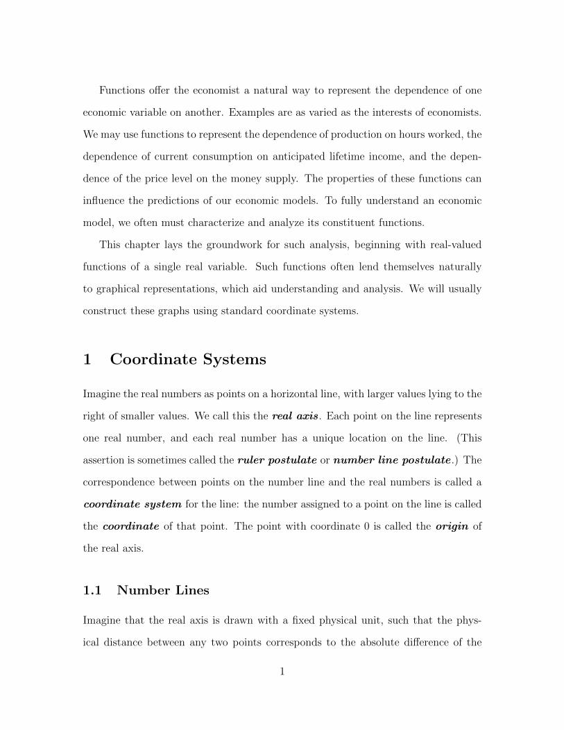
1.1 Number Lines

Imagine that the real axis is drawn with a fixed physical unit, such that the phys-

ical distance between any two points corresponds to the absolute difference of the

1

-5 -4 -3 -2 -1 0 1 2 3 4 5[ ]( )

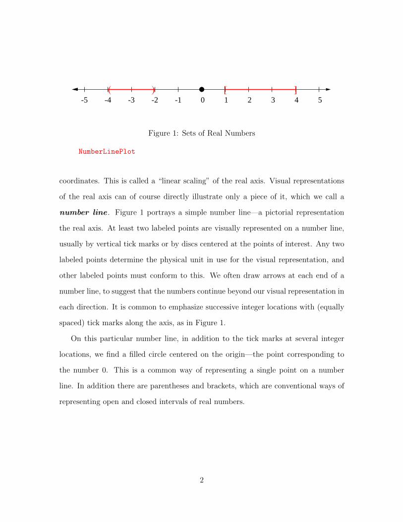
Figure 1: Sets of Real Numbers

NumberLinePlot

coordinates. This is called a “linear scaling” of the real axis. Visual representations

of the real axis can of course directly illustrate only a piece of it, which we call a

number line . Figure 1 portrays a simple number line—a pictorial representation

the real axis. At least two labeled points are visually represented on a number line,

usually by vertical tick marks or by discs centered at the points of interest. Any two

labeled points determine the physical unit in use for the visual representation, and

other labeled points must conform to this. We often draw arrows at each end of a

number line, to suggest that the numbers continue beyond our visual representation in

each direction. It is common to emphasize successive integer locations with (equally

spaced) tick marks along the axis, as in Figure 1.

On this particular number line, in addition to the tick marks at several integer

locations, we find a filled circle centered on the origin—the point corresponding to

the number 0. This is a common way of representing a single point on a number

line. In addition there are parentheses and brackets, which are conventional ways of

representing open and closed intervals of real numbers.

2

1.1.1 Intervals

Recall that a set is just a collection of distinct objects, which are called the elements

of the set. (See the sets chapter for more detail.) We denote the entire set of real

numbers by R, and if x is a real number we can write x ∈ R to say concisely that x

is in the set R.

We can use a number line to pictorially represent simple sets of real numbers. For

example, consider the set of all real numbers greater than or equal to 1 but less than

or equal to 4. This is a subset of the real numbers, which we can represent in set

notation as {x ∈ R | 1 ≤ x ≤ 4}. We call this the closed interval from 1 to 4.1 We

will generally use the interval notation [1 .. 4] to denote this set. The numbers 1 and

4 are called the endpoints of this interval: a closed interval includes its endpoints.

Such a closed interval is an example of a line segment . You will find the interval

[1 .. 4] represented in Figure 1 by a line segment with a closing bracket at each end.

The square brackets are used to indicate that the endpoints are part of the interval.

Now consider the set of real numbers greater than −4 but less than −2, which we

can write in set-builder notation as {x ∈ R | −4 < x < −2}. We call this the open

interval from −4 to −2. We will represent this with the interval notation (−4 ..−2).

You will find this set represented in Figure 1 by a line segment with a parenthesis

at each end. The numbers −4 and −2 are still called the endpoints of the interval,

but an open interval does not contain its endpoints. Parentheses are used to indicate

that the endpoints are not part of the interval.

1See the analysis chapter for a more detailed discussion of open and closed sets.

3

1.2 Rectangular Coordinates

Draw two number lines in the plane, perpendicular to each other and intersecting

at their origins. From these we can produce a rectangular coordinate system for the

plane. We will call the two number lines the coordinate axes of the coordinate

system. By convention, one axis is horizontal and the other vertical. Any point in

the plane can be represented as an ordered pair, called the coordinates of the point.

We list the coordinates as an ordered pair. (The first coordinate is sometimes called

the abscissa ; the second is sometimes called the ordinate .)

In the standard rectangular coordinate system, the first coordinate is the coordi-

nate on the horizontal axis. (This is the distance from the vertical axis.) The second

coordinate is the coordinate on the vertical axis. (This is the distance from the hor-

izontal axis.) Equivalently, we project the point perpendicularly onto each axis in

order to determine the point’s coordinates. The point (0, 0) is called the origin of

this coordinate system.

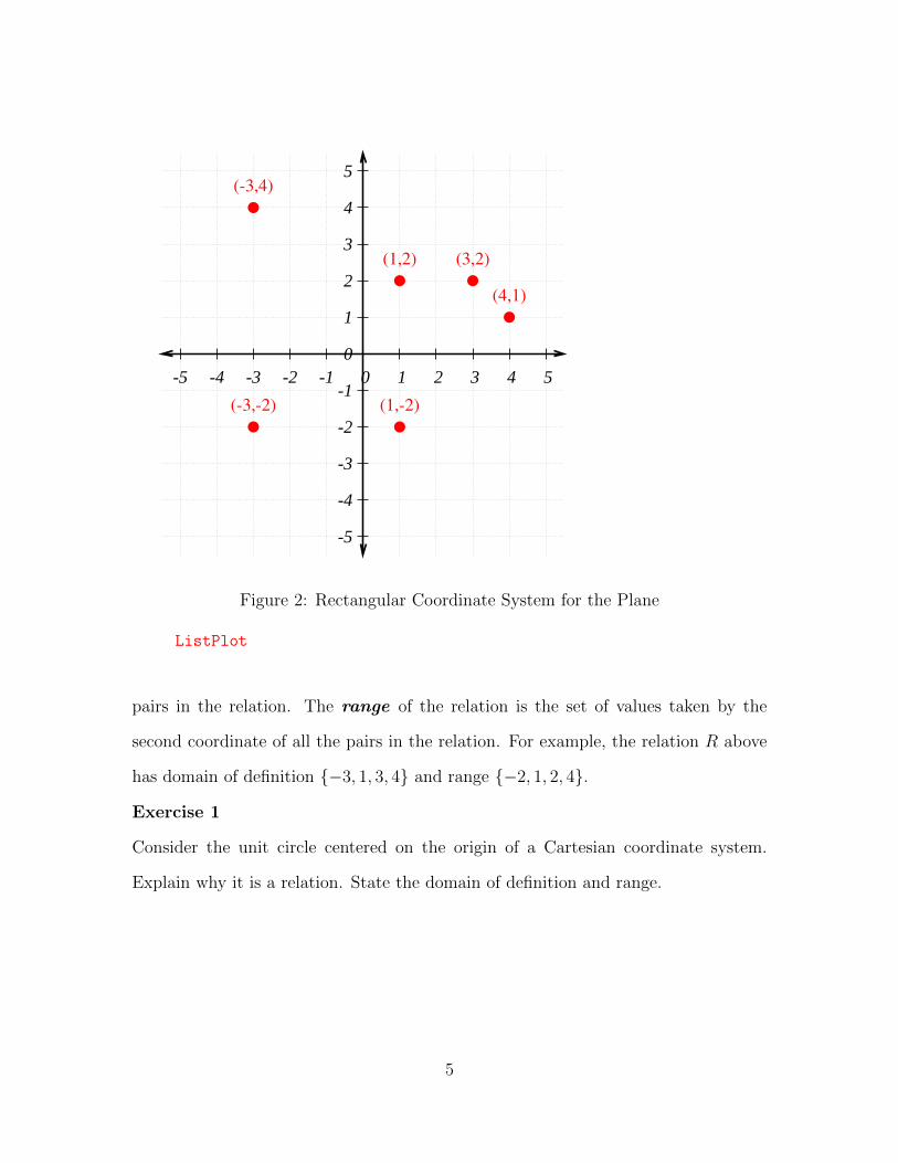
Figure 2 displays a rectangular coordinate system for the plane. A few points are

plotted, and they are labeled with their coordinates. Any set of ordered pairs is a

relation . (See the relation chapter for a fuller discussion of relations.) So the set

of all the ordered pairs labeled in Figure 2 is a relation. In such very simple cases

we can write the relation explicitly by listing its elements. For example, suppose we

define the set R as the following set of ordered pairs.

Rdef= {(−3, 4), (−3,−2), (1, 2), (1,−2), (3, 2), (4, 1)} (1)

Then R is the relation illustrated in Figure 2.

Remember a relation is a set of ordered pairs. Order matters. The domain of

definition of the relation is the set of values taken by the first coordinate of all the

4

-5

-4

-3

-2

-1

0

1

2

3

4

5

-5 -4 -3 -2 -1 0 1 2 3 4 5

(1,2) (3,2)

(4,1)

(-3,-2) (1,-2)

(-3,4)

Figure 2: Rectangular Coordinate System for the Plane

ListPlot

pairs in the relation. The range of the relation is the set of values taken by the

second coordinate of all the pairs in the relation. For example, the relation R above

has domain of definition {−3, 1, 3, 4} and range {−2, 1, 2, 4}.

Exercise 1

Consider the unit circle centered on the origin of a Cartesian coordinate system.

Explain why it is a relation. State the domain of definition and range.

5

2 Functions

A function is a special kind of relation: it maps each element of the domain to a unique

element in the codomain.2 Equivalently, for each input (from the domain) the func-

tion produces a unique output (in the codomain). Economic objectives, behavioral

responses, and production technologies are often expressed as functions. Examples

include money demand functions, consumption functions, production functions, util-

ity functions, commodity demand functions, inverse commodity demand functions,

oligopoly reaction functions, and many other economic relations.

Example 1

The relation R illustrated in Figure 2 is not a function, since some elements in the

domain of definition map to multiple elements in the range. One problem is that

(−3,−2) and (−3, 4) are both in R. The point −3 in the domain maps to points −2

and 4 in the range. Another problem is that (1,−2) and (1, 2) are both in R. The

point 1 in the domain maps to points −2 and 2 in the range.

Definition 2.1 (Function) The domain of a function is the set of valid inputs

for that function. The codomain of a function is the set of all valid outputs of

the function. A function pairs each point in the domain with only one point in the

codomain. (I.e., it is left-total and right-definite.)

The notation Xf→ Y indicates that X is the domain and Y is the codomain of the

function named f . A common equivalent notation is f : X→ Y. We also say that f

is a function from X to Y. (When a function has a codomain that is identical to its

domain, we may call it a function in the set.) Computational discussions often call

X → Y the type signature of the function, where X is the argument type and Y

is correspondingly the return type of the function.

2See the relation chapter for a additional discussion of functional relations.

6

We often think of a function as embodying a rule for turning inputs into unique

outputs. Consider a value x in the domain of the function f . For any x in the do-

main, let f(x) represent the value of f at x. This use of parentheses is the most

common mathematical notation for function application , and it is also a fairly com-

mon synatx in programming languages. (However, the syntax for function application

varies across mathematical presentations and varies widely across programming lan-

guages.)

We usually read f(x) simply as “f of x” or “f applied to x”, but we may also say

“the image of x under f .” A common way to express the idea that the function f

maps a particular argument value x to a particular return value y is by means of the

equality y = f(x), where y is the corresponding value y in the range of the function.

We then say that y is the image of x under f . The set of all the image points is

called the range of the function, which may be written as f(X).

Function definition typically involves expressions in variables. For example, it is

common to state that a real function f has a return value that is the square of its input

argument by writing f(x) = x2. Almost as common is to write f = x 7→ x2, where

arrow is read as “maps to”. (The words mapping and map are common synonyms

for function.) Both notations are meant to associate a name f with a function, but

the second notation more cleanly separates naming from function specification: we

assign the function (x 7→ x2) to the name f . Having an anonymous notation for

functions can be convenient; for example, it allows us to talk about a particular

function without bothering to assign it a name.

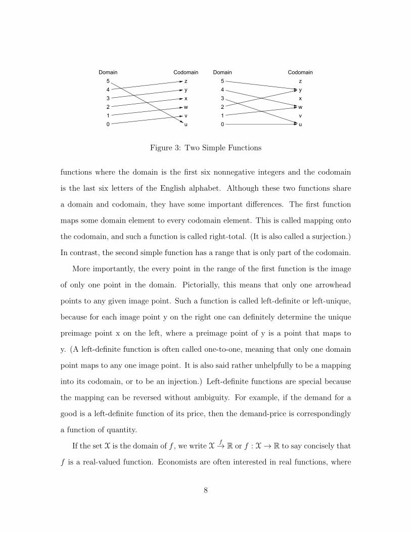
Very simple functions may be depicted as arrows from the elements of the domain

to the corresponding elements of the codomain. Each arrow links two points: the

domain point is called a preimage of the codomain point, and the codomain point is

called the image of the domain point. As an example, Figure 3 presents two simple

7

0

1

2

3

4

5

u

v

w

x

y

z

Domain Codomain

0

1

2

3

4

5

u

v

w

x

y

z

Domain Codomain

Figure 3: Two Simple Functions

functions where the domain is the first six nonnegative integers and the codomain

is the last six letters of the English alphabet. Although these two functions share

a domain and codomain, they have some important differences. The first function

maps some domain element to every codomain element. This is called mapping onto

the codomain, and such a function is called right-total. (It is also called a surjection.)

In contrast, the second simple function has a range that is only part of the codomain.

More importantly, the every point in the range of the first function is the image

of only one point in the domain. Pictorially, this means that only one arrowhead

points to any given image point. Such a function is called left-definite or left-unique,

because for each image point y on the right one can definitely determine the unique

preimage point x on the left, where a preimage point of y is a point that maps to

y. (A left-definite function is often called one-to-one, meaning that only one domain

point maps to any one image point. It is also said rather unhelpfully to be a mapping

into its codomain, or to be an injection.) Left-definite functions are special because

the mapping can be reversed without ambiguity. For example, if the demand for a

good is a left-definite function of its price, then the demand-price is correspondingly

a function of quantity.

If the set X is the domain of f , we write Xf→ R or f : X→ R to say concisely that

f is a real-valued function. Economists are often interested in real functions, where

8

both the domain and the codomain are subsets of the real numbers. If the domain X

is all of the real numbers, we simply write R f→ R or f : R→ R. This means that f

maps each real number to a real number.

Definition 2.2 (Real Function) A function of a real variable has a domain

that is a set of real numbers. A real-valued function has a codomain that is a set

of real numbers. A real-valued function of a real variable is called a real function.

(Occasionally, for additional clarity, we may call it a real-to-real function.)

Example 2 (Real Identity)

One of the simplest real functions is the real identity function: (x 7→ x). Its domain

and codomain are the real numbers. It is left definite and right total.

Part of the characterization of any function is a specification of its valid inputs.

Recall that all permitted values for the inputs constitute the domain, or argument

type, of the function. Very often we do not state the domain explicitly, in which case

we will assume that it is the largest sensible domain. In particular, a real function

is considered to have a natural domain of the set of real numbers x for which f(x)

is a real number. For example, if we are interested in the real function (x 7→ x2),

the natural domain is the set of real numbers (R). (This is true for any polynomial.)

But consider the function characterized by the rule (x 7→ 1/x); clearly we must omit

x = 0 from the natural domain.

In economics, functions often have a domain of economic relevance, which may

be much smaller than the natural domain. Even when R is the natural domain of

a function, in an economic model the domain is often restricted to the nonnegative

real numbers (R+). We will sometimes refer to the restricted domain determined by

economic considerations as the economic domain.

9

Example 3 (Linear Consumption)

Real consumption per capital (c) is correlated with real disposable income per capita

(y). We might abstractly represent a theory that there is an underlying functional

dependence by writing c = f(y). Economists turn to the data to search for plausible

defining expressions for f . Suppose that consumption and income data suggest that

this relation is approximately

c = 20 + 0.8y

Then the real function y 7→ 20+0.8y represents our consumption function. Its domain

and codomain are typically the nonnegative real numbers. It is left definite.

10

Example 4 (Simple Production Function)

Treating all other inputs as constant, we might propose that Y = f(N). That is,

there is a functional dependence of output produced, Y , on the labor input, N . This

says that for each value of labor input (N) there is a unique value of output (Y )

that is produced. In this case, N may be the independent variable (i.e., the function

input), Y may be called the dependent variable (i.e., the function output), and f is

an example of a production function. Ruling out, e.g., power-loom riots, the possible

values of the labor input are generally nonnegative. That is, the economic domain of

the function is the set of non-negative real numbers (R+).

Empirical or theoretical considerations may suggest a specific representation of

the transformation of labor N into final output Y . To give a very simple example,

consider

f(N)def= 100 ·N

To the right of the equals sign is the defining expression for the function: the value of

f at N is defined to be 100 ·N . Using this definition, we represent the transformation

of labor N into final output Y by the equation

Y = 100 ·N

In this special case, the average product of labor (Y/N) is a constant.

2.1 Defining Functions for Computing

Code duplication reduces both readability and maintainability. In order to avoid such

duplication, programmers develop subroutines that can be reused whenever needed.

(This observation supports the popular DRY principle: don’t repeat yourself.) Ev-

ery modern programming language therefore provides facilities for code reuse, and

11

computational functions are a particularly important example. Function definitions

contain code that can be executed repeatedly during a single execution of the main

program. In other words, functions are a way to package subroutines for easy reuse.

Functions have broad application in programming.

In a computational context, the term function often receives a very broad use: it

may refer to any callable subroutine. Whereas a mathematical function has a clearly

defined domain and codomain, a computational function may not. Whereas a mathe-

matical function simply maps any valid input to a value in its range, a computational

function may not even return an output value. (The term procedure is often used

when there is no explicit output.) A computational function may even accept no

input and yet return a value, as with traditional random number generators.3 Even

when it does accept an input argument, a computational function may not restrict

the function behavior to ensure that it handles only valid inputs.

However, some computational functions behave very much like mathematical func-

tions. When the output value of a computational function is completely determined

by its input arguments, it is a pure function. Pure functions are very useful: they

make it much easier to read and understand what is happening in a program. It also

makes it easier to relate the behavior of computer code to mathematical constructs,

since mathematics deals in pure functions. It is a good programming habit to work

with pure functions whenever doing so proves reasonably convenient. Nevertheless,

impure computational functions can be very useful for their side effects. (For ex-

ample, an impure function may change the global program state, or change the state

of a program object, or simply print a description of the object state.)

Listing 1: Function Definition

Function consume ( yd ) :

3Random number generation is discussed in the sequence chapter.

12

spending ← 20 + 0 .8 · ydreturn spending

Listing 1 introduces the somewhat formal style of pseudocode we will use to define

named functions. (Pseudocode is a stylized description of what you need to implement

in your chosen language; your actual code may look very different.) We begin with

a function-definition header that gives the function a name and specifies names for

the input arguments. (These names are often called the formal parameters of the

function.)4 A formal parameter is a name we use to refer to the input argument. In

this case the function is named consume, and it takes a single input argument, named

yd. Indented code following the function-definition header constitutes the body of

the function. For maximum readability, we delimit the function body with simple

indentation.5 Also, each line after the function-definition header contains a single

statement; we do not delimit these statements in any other ways.

We use the input argument in the body of the function: the value of total con-

sumption spending is computed based on disposable income, This computed value is

assigned to spending. (As this example illustrates, in our pseudocode we will simply

bind names to values on an as needed basis.) The return statement specifies that the

value of spending is returned when the function is called. In order for this compu-

tational function to produce a value, we must apply it to a specific input argument

(i.e., a specific value for yd). This process is often described as a function call. For

example, consume(50) calls the function with an input argument of 50, to the return

value will be 60. As in this example, the pseudocode in this book often will not specify

the precise type of the values in our computations. Here we are satisfied to indicate

4We assume formal parameters are inaccessible from outside of the function definition; they havelocal scope. Similarly, variables introduced in the function definition are assumed to have localscope. In some languages, scope must be explicitly restricted.

5We will always use simple indentation to delimit code blocks; we will never use braces or keywordsfor such delimitation.

13

by context that a function call requires a numerical input and returns a numerical

result.

Example 5

Here are some examples of implementation of Listing 1 in different languages. (For

the purposes of illustration and comparison, in each case we insist on an assignmentto a local variable named spending.)

Python:

def consume ( yd ) :spending = 20 + 0 .8 * ydreturn spending

Mathematica:

consume = Function [ yd ,Module [{ spending } ,

spending = 20 + 0.8* yd] ]

C:

double consume (double yd ) {double spending ;spending = 20 + 0 .8 * yd ;return spending ;

}

This book assumes that computational functions are first-class citizens of their

programming language. This means that programmers can treat them like any other

values in the language (e.g., assign them to variables or pass them to functions). This

treatment of functions was oddly slow to arrive in programming languages, but in the

21st century it is a common language feature.

14

2.2 Operations on Functions

Consider two real functions, R f→ R and R g→ R. For any real numbers α and β,

define a linear combination αf + βg by

(αf + βg)(x)def= α · f(x) + β · g(x) (2)

A linear combination of f and g is a new real function. A special case is the addtion

of real functions, which is particularly easy to visualize graphically since it is just the

vertical addition of the two component functions.

We can similarly define the product f ·g of the functions by (f ·g)(x) = f(x) ·g(x).

As an additional bit of notation, let −f = −1 · f . Division is a bit trickier, because

we need to avoid division by 0. If the range of g does not include 0, we can define

f/g by (f/g)(x) = f(x)/g(x).

There is one more operation on these functions that is of particular interest: the

operation of function composition. Define f ◦ g by

(f ◦ g)(x)def= f(g(x)) (3)

We often build up computations as the composition of simple functions.

Example 6

Define the real function sq = x 7→ x2. Use function composition to define

sin2 = sq ◦ sin

cos2 = sq ◦ cos

The real function sin2 computes the sine of its argument and then squares it. Thereal function cos2 computes the cosine of its argument and then squares it. You mayrecall that 1.0 is always the return value for the real function sin2 + cos2.

15

Composition is a binary operation on functions: with an input of two functions,

its return value is a new function. Let iR represent the identity function on the real

numbers. This function naturally serves as an identity for function composition. That

is, give the real function f : R→ R, The

iR ◦ f = f

f ◦ iR = f

To see this, note that by definition (iR ◦ f)(x) = iR(f(x)) = f(x) and (f ◦ iR)(x) =

f(iR(x)) = f(x).

One useful property of function composition is associativity:

(f ◦ g) ◦h = f ◦(g ◦h) (4)

To see this, note that by definition ((f ◦ g) ◦h)(x) = (f ◦ g)(h(x)) = f(g(h(x))) and

(f ◦(g ◦h))(x) = f((g ◦h)(x)) = f(g(h(x))). As a result, we can drop the parenthesis

and just write f ◦ g ◦h, without fear of ambiguity.

A function in a set may be composed with itself. (This is called function iteration.)

Let f be a function in X and let iX be the indentity function on this set. Define

f ◦n =

iX for n = 0

f ◦ f ◦(n−1) for n = 1, 2, . . .

(5)

Since composition is associative, we might write this as

f ◦n = f ◦ f ◦ . . . ◦ f︸ ︷︷ ︸n times

(6)

16

This definition implies the following two index laws :

f ◦(n+m) = f ◦n ◦ f ◦m

f ◦nm = (f ◦n)◦m(7)

Example 7

Define the real function f = (x 7→ 2x). Then f ◦ 2 = (x 7→ 4x) and f ◦ 3 = (x 7→ 8x).

Additionally

f ◦ 2 ◦ f ◦ 3 = f ◦(2+3) = (x 7→ 32x)

(f ◦ 2)◦ 3 = f ◦(2·3) = (x 7→ 64x)

3 Difference Quotient

Consider a real function f and some nonzero constant h, and define a new function

g by g(x) = f(x + h). The new function is called a discrete shift of f , and

the constant h is the stepsize of the discrete shift. The delta operator ∆h similarly

produces a new function, which is the difference between the shifted function and the

original function. That is,

(∆hf)(x) ≡ f(x+ h)− f(x) (8)

It is conventional to drop the first parentheses and write the step-h difference delta

of the function f at the point x as ∆hf(x). If h > 0, we call the result a forward

difference at x. If h < 0, we call the result a backward difference at x.

Exercise 2

Prove that ∆hk = 0 for any constant k. Prove that ∆hx = h. Prove that ∆h is linear.

17

That is, given real functions f and g, and real constants α and β, show that

∆h(αf + βg) ≡ α∆hf + β∆hg

Exercise 3

For any integer n > 0, show that ∆hxn is a polynomial of degree n− 1.

A step-h difference quotient for a real function f is just the ratio of the step-h

difference delta and the step size. Given f : R → R and a nonzero h, the difference

quotient is well-defined.

Definition 3.1 (Difference Quotient) Let f be a real function. Let x and x + h

be two distinct points in the domain. The step-h difference quotient for f at x is

qhf(x) =f(x+ h)− f(x)

h

Given the real function f and the stepsize h, the difference quotient qhf is a new

real function. If h > 0, it is a forward difference quotient. If h < 0, it is a

backward difference quotient. (The difference quotient is not defined for h = 0;

the dcalc chapter addresses this in more detail.)

Recall that a secant line to a function is a line that passes through two function

points, such as (x, f(x)) and (x′, f(x′)). So given f and h, the difference quotient is

a function that returns secant slopes for f . To make this explicit, define x′def= x+h.

Then

f(x+ h)− f(x)

h=f(x′)− f(x)

x′ − x

In general, this secant slope will vary if we change x or x′. That is, the value of a

difference quotient for a function varies as the input varies. In the special case of

affine functions, the difference quotient is constant.

18

Definition 3.2 (Affine Function) Let f be a real function. If f(x) = a0 + a1x for

constants a0 and a1, we say that f is affine . If in addition a0 = 0, we say that f is

linear .6

Exercise 4

Show that the difference quotient of an affine function does not depend on the choice

of points for its computation.

Example 8

Revisit the consumption function c = (y 7→ 20+0.8y) to compute a difference quotient

at the point y1 with stepsize h.

c(y1 + h)− c(y1)

h=

(20 + 0.8(y1 + h))− (20 + 0.8y1)

h= 0.8

The value of the difference quotient does not depend on x or on h.

Example 9

Let f = (x 7→ x2). Given x and h, compute the difference quotient as

qhf(x) =(x+ h)2 − x2

h=

2xh+ h2

h= 2x+ h

The value of the difference quotient depends on x and on h.For any given value of x, the difference quotient depends on h. For example, given

x = 2, we find qhf(2) = 4+h. The value of the difference quotient depends on both thesize and the sign of h. With x = 2 and h = 1, we find a forward difference q1f(2) = 5;With x = 2 and h = −1, we find a backward difference q−1f(2) = 3. With a smallerstepsize, the difference between the foward difference and the backward difference issmaller.

Listing 2 illustrates a simple function to computate a difference quotient, which

depends on a reference point x and a step size h. Once again we rely on a semi-formal

6Affine functions are sometimes casually called linear, because the graph of an affine function is astraight line. In the true linear case, when a0 = 0, the value of the function is directly proportionalto the argument. In this case, the slope a1 becomes a constant of proportionality , and the graphof the function passes through the origin.

19

Listing 2: Difference Quotient

Function d i f f e r enc eQuot i en t ( f , x , h ) :#t y p e : ( C a l l a b l e , Real , Rea l ) → Rea l

df ← f ( x + h) - f ( x ) #change o f v a l u e o f f

return df/h #v a l u e o f d i f f e r e n c e q u o t i e n t

pseudocode. There are a few features to notice. Comments are typographically dis-

tinguished from the code. This function has multiple input arguments: the function

whose difference quotient we are computing, a reference point for the difference quo-

tient, and a step size for the difference quotient. The pseudocode assumes functions

can be passed like any other object.7

We have added a few annotations to this pseudocode, including a type hint for

each input argument (in parentheses) and a type hint for the return value (after a

right arrow). A type hint of Callable means the type ordinarily used in the language

to represent a function. A type hint of Real means the type ordinarily used in the

language to approximately represent a real number. (This is usually a floating point

number.)

Some languages rigidly require that type information be provided for all input

and output arguments. Some languages do not provide any facilities for specifying

type information. And in some languages, the specification of type information is

partially or entirely optional. In this book, type hints are provided on an ad hoc

basis, according to how helpful we deem it to provide them in a particular context.

7Many languages do not include this useful feature. Those that do are said to treat functions asfirst class citizens, or equivalently, to have first-class functions (Strachey, 2000).

20

3.1 Interpreting the Difference Quotient

Roughly speaking, a real function f is continuous if one can imagine drawing it

on paper without lifting our pencil. (See section 5 for more details.) The difference

quotient of a continuous function represents an average rate of change.

3.1.1 Secants

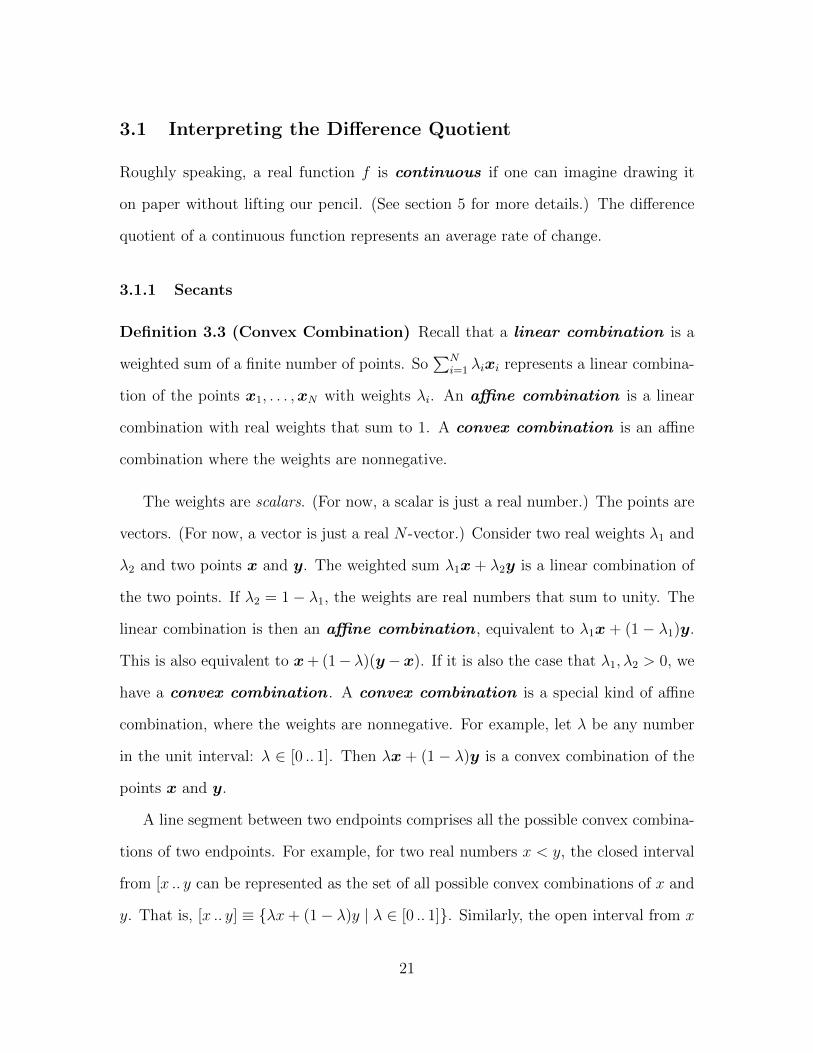
Definition 3.3 (Convex Combination) Recall that a linear combination is a

weighted sum of a finite number of points. So∑N

i=1 λixi represents a linear combina-

tion of the points x1, . . . ,xN with weights λi. An affine combination is a linear

combination with real weights that sum to 1. A convex combination is an affine

combination where the weights are nonnegative.

The weights are scalars. (For now, a scalar is just a real number.) The points are

vectors. (For now, a vector is just a real N -vector.) Consider two real weights λ1 and

λ2 and two points x and y. The weighted sum λ1x + λ2y is a linear combination of

the two points. If λ2 = 1− λ1, the weights are real numbers that sum to unity. The

linear combination is then an affine combination , equivalent to λ1x + (1 − λ1)y.

This is also equivalent to x+ (1− λ)(y−x). If it is also the case that λ1, λ2 > 0, we

have a convex combination . A convex combination is a special kind of affine

combination, where the weights are nonnegative. For example, let λ be any number

in the unit interval: λ ∈ [0 .. 1]. Then λx + (1 − λ)y is a convex combination of the

points x and y.

A line segment between two endpoints comprises all the possible convex combina-

tions of two endpoints. For example, for two real numbers x < y, the closed interval

from [x .. y can be represented as the set of all possible convex combinations of x and

y. That is, [x .. y] ≡ {λx+ (1− λ)y | λ ∈ [0 .. 1]}. Similarly, the open interval from x

21

to y can be represented by {λx+ (1− λ)y | λ ∈ (0 .. 1)}.Exercise 5

Let f be a real function, and let p1 = (x1, f(x1)) and p2 = (x2, f(x2)) be two points

of the function. Use (9) to show that any point p = (x, y) on the associated secant

segment between p1 and p2 can be written as a convex combination of the two points.

That is, show that there is some λ ∈ [0 .. 1] such that x = λx1 + (1 − λ)x2 and

y = λf(x1) + (1− λ)f(x2).

A secant line of the function f is a line that passes through any two distinct

points of the function. (The word ‘secant’ derives from the Latin word ‘secare’, which

means “to cut”.) A secant segment is the line segment between two such points.

Let x and x′ be two distinct points in the domain of f . Then we can draw a straight

line through the two points (x, f(x)) and (x′, f(x′)). This is a secant line, which

includes the secant segment between the two points.

3.1.2 Difference Quotients as Slopes

A difference quotient is just the slope of a secant line. For example, the difference

quotient for f from x to x + h is the slope of the secant line through (x, f(x)) and

(x+ h, f(x+ h)). Equivalently, it is the slope of the secant segment from (x, f(x)) to

(x+ h, f(x+ h)). If our function is continuous over the closed interval [x .. x+ h], we

can interpret this difference quotient as the average rate of change in the value

of f .8

Figure 4 illustrates the graph of a function, a secant line passing through two

points of the function graph, and a corresponding secant segment that has these two

points as endpoints. Note that the secant line is a straight line. As a result, we can

choose any two points along this secant line and we will compute the same difference

8Here h > 0; we have a forward difference.

22

f(x1)

f(x0)

x1x0

f(x)secant line

x1-x0

f(x 1

) -

f(x 0

)Figure 4: A Secant Segment Implies a Difference Quotient

quotient. This is not true of the nonlinear function we plotted: since it is not a

straight line, the value of the difference quotient will depend on which two points we

choose.

Suppose for some function f we compute the difference quotient m = qf (x0, h).

Then we can write the equation for the secant line as

y = f(x0) +m · (x− x0) (9)

If we restrict the domain to the interval between x0 and x0 + h, this same equation

gives us the equation for the secant segment.

We wrote the equation for the secant line in point-slope form, using the point

23

(x0, f(x0)). The difference quotient for any two points on this line is constant. This

constant value is the slope of the line, and it tell us the amount by which the dependent

variable y must change for each unit change in the independent variable x. That is, it

is the rate of change of y in terms of x. Corresponding to this, the difference quotient

qf (x0, h) gives us the average rate of change of f over the interval between x0 and

x0 + h. Economists often refer to rates of change as “marginal” quantities.

Example 10

Consider the linear consumption function

c = 20 + 0.8y

This is an affine function, so it has a constant difference quotient. The difference

quotient is the rate change in c given a unit change in y, which we call the marginal

propensity to consume out of income.

Consider a firm facing the following costs of producing a quantity Q of its good:

TC = 100 + 20Q

The total cost of production (TC) comprises fixed costs (100), which do not vary

with the level of production, and variable costs (20Q), which vary with the level of

production. We see that each unit of additional output adds 20 to the total cost of

production (or equivalently, to the variable cost of production). This is the rate at

which costs increase with production, so 20 is the marginal cost of production.

3.2 Average and Marginal

For many economically interesting functions, we are interested the average value of the

function per unit of its argument. (For example, we may be interested in the average

24

product of labor.) The average value often has a good economic interpretation when

we have a nonnegative function of a positive real variable. For example, if we have

f : R++ → R++, we can construct the average as f(x)/x. (Of course we cannot

compute an average function value for a zero input,) We can interpret this average

value as the slope of a line from the origin to the point (x, f(x)). A natural question

is whether this average value is increasing or decreasing. The answer is given by the

relationship between the average value and the marginal value.

Given f : R++ → R++ and x′ > x > 0, we now consider whether the average

value of f increases when its argument increases from x to x′. Suppose the marginal

value is currently greater than the average value:

f(x′)− f(x)

x′ − x >f(x)

x(10)

For x′ > x, this implies that

x f(x′) > x′ f(x) (11)

or equivalently

f(x′)

x′>f(x)

x(12)

While the marginal value exceeds the average value, the average value is an increasing

function. Symmetrically, while the average value exceeds the marginal value, the

average value is a decreasing function.

3.2.1 Sum Rule

Suppose f is a real function, and so is g. We can construct a new function, h,

according to the rule:

h(x) = f(x) + g(x) (13)

25

We call h the sum of f and g. Note that the difference quotient of h is just the sum

of the difference quotient of f and the difference quotient of g.

qh(x, dx) =h(x+ dx)− h(x)

dx

=[f(x+ dx) + g(x+ dx)]− [f(x) + g(x)]

dx

=f(x+ dx)− f(x)]

dx+g(x+ dx)− g(x)

dx

= qf (x, dx) + qg(x, dx)

(14)

The sum rule for difference quotients, which says that h = f + g =⇒ qh(x, dx) =

qf (x, dx) + qg(x, dx), makes perfect intuitive sense. Starting from h(x), a change dx

in the input argument lead to a change in the value of h for two reasons: f changes,

and g changes. Since h = f + g, the change in the value of h is the sum of the change

in the value of f and the change in the value of g.

4 Monotone Functions

A monotone function is one whose value is always rising or always falling. The

following definition makes this more precise.

Definition 4.1 (Monotone Functions) We say a function f is increasing iff9

x′ ≥ x =⇒ f(x′) ≥ f(x)

9This book uses the terms increasing and decreasing as synonyms for the less familiar termsisotone and antitone . Also, for notational simplicity, the ordering in the domain and the orderingin the codomain use the same comparion operator symbol. (In the background are two ordered sets,(X,≥X) and (Y,≥Y), and a function f : X→ Y. See the relation chapter for a discussion of orderedsets.)

26

If an increasing function satisfies

x′ > x =⇒ f(x′) > f(x) (15)

it is strictly increasing . We analogously define decreasing and strictly de-

creasing by reversing the right-hand-side inequalities. If a function is increasing or

decreasing, it is monotone . If a function is strictly increasing or strictly decreas-

ing, it is strictly monotone . A monotone function that is not strictly monotone

is sometimes called weakly monotone . A slight oddity of this definition is that a

constant function is monotone: indeed, it is both increasing and decreasing.

A function f that is not monotone may nevertheless be monotone on portions of

its domain. If we have an subset of the domain over which f is monotone, then we

say that f is monotone on that subset. (For example, x 7→ x2 is strictly increasing

on the nonnegative real numbers.)

Economists often care about functions that are strictly monotone: either strictly

increasing or strictly decreasing over their entire domain. For strictly increasing

functions, we may say that the order in the domain is preserved in the range. For

example, utility functions are often strictly increasing in the level of consumption,

production functions are often strictly increasing in input levels, and price indexes

are increasing in their constituent prices.

Example 11

Consider again the consumption function defined by the equation c = 20 + 0.8y.

Taking any two points of the function, (y1, c1) and (y2, c2), we see that y2 > y1

implies c2 > c1. So the function is strictly increasing.

27

Example 12 (CDF)

A cumulative distribution function FX(x) gives for each value x the probability that

the random variable X will take on a value less than or equal to x. That is,

FX(x) = P (X ≤ x)

Since this probability cannot decline as x increases, FX must be increasing.

Theorem 1

Let f be a real function. The function f is increasing iff the difference quotient

is always nonnegative and is strictly increasing iff the difference quotient is always

positive. Similarly, the function f is decreasing iff the difference quotient is always

nonpositive and is strictly decreasing iff the difference quotient is always negative.

Exercise 6

Prove theorem 1.

4.1 Functions with Inverses

Recall that a function is essentially a collection of ordered pairs. So we can always

construct an inverse relation for any function: just reverse the order of every ordered

pair belonging to the function.

Definition 4.2 (Inverse Relation) Given the function Xf→ Y, we construct the

inverse relation f−1 by reversing all the ordered pairs in f , so that (y, x) ∈

f−1 ⇐⇒ (x, y) ∈ f .

28

Example 13

Use the rule x 7→ x2 to define a function f from {−1, 0, 1} to {−1, 0, 1}. This gives

use three points in f : (−1, 1), (0, 0), and (1, 1). The inverse relation f−1 therefore

also comprises three points: (1,−1), (0, 0), and (1, 1).

Since the domain of f−1 is {−1, 0, 1}, but −1 is not mapped to any value, f−1 is

not a function. Furthermore, since f−1 maps 1 to −1 and to 1, it is not a function.

The inverse relation for a function may not be a function. We now introduce some

terminology that will help us characterize the situations in which the inverse relation

is a function.

Definition 4.3 (One-to-One) Consider a function f with domain X and codomain

Y. Since f is a function, the image of x under f is a single point in Y. For some

functions it is also true that each point in the range of f is the image of a unique

point in the domain. That is, f(x) = f(x′) =⇒ x = x′. We call such a function

one-to-one . (Synonymously, the function is an injection .)

Definition 4.4 (Onto) Consider a function f with domain X and codomain Y. For

any subset S of the domain, we define f(S) to be the associated elements in the

codomain of f . (That is, ∀S ⊆ X, f(S)def= {y | ∃x ∈ S s.t. y = f(x)}.) We call

f(S) the image of S under f . The image of the entire domain, f(X), is called the

range of f . Generally the range will be a subset of the codomain, but if they are

equal the we say the function is onto. (Synonymously, the function is a surjection .)

Definition 4.5 (Bijection) A function is a bijection is it is one-to-one and onto.

Given the function Xf→ Y, the inverse relation has domain Y and codomain X.

We can ask, under what conditions is f−1 also a function? The answer is that f−1 is

a function iff f is a bijection.

29

The requirement that f be one-to-one is obvious, for otherwise f−1 will map a

single point in its domain to more than one in its codomain. The requirement that

f be onto is perhaps less obvious, until we recall that by definition a function maps

every point in its domain to a point in its codomain. Remember, if X and Y are the

domain and codomain of f , then Y and X are the domain and codomain of f−1.

However if f is one-to-one but not onto, the inverse relation is still a function on

a subset of Y. (That is, f−1 : f(X) → X is a function.) The difference is just the

domain of f−1: we need to restrict it to the range of f , which is a subset of Y when f

is not onto. It is therefore somewhat common to say loosely that f−1 is an inverse

function whenever f is an injection. (When we want to be very clear that f−1 may

not be defined on all of Y, we call it a functional relation or partial function.)

Suppose f is a real function. If f is strictly monotone, then it is one-to-one, so the

inverse is a functional relation. (See definition 4.2.) In this case, f−1 is also strictly

monotone.

Example 14

Consider the real function defined by the following equation: y = 3√x. This is a

strictly increasing function, so it has an inverse. For each pair (x, y) of the original

function f , a corresponding pair (y, x) belongs to the inverse function f−1. That is,

the inverse function is a reflection of the original function through the 45◦ line. So

we can represent the inverse function by the equation x = 3√y or equivalently y = x3.

Figure 5 illustrates this case.

30

0

0

x

f(x)

f−1(x)

Figure 5: Inverse of Function as Reflection

Example 15 (Inverse Demand)

Suppose the equation Q = 1000− 5P represents consumer demand for a good. This

tells us that quantity demanded is a strictly decreasing function of price. For example,

if P rises from 80 to 100, then Q falls from 600 to 500. Therefore we can solve for P

as a function of Q, to get the inverse demand function: P = 200−Q/5. This tells us

that the market price is a strictly in the quantity sold. For example, if Q rises from

500 to 600, then P falls from 100 to 80.

31

Example 16 (Giffen Goods)

Suppose Q = f(P ) represents a consumer’s purchase of a good: the quantity de-

manded is a function of the price of that good. Economists often find it convenient

to work with the inverse demand function: P = f−1(Q). This works fine if the good

obeys the law of demand , which states that demand is strictly decreasing in price.

A Giffen good is an inferior good where income effects so outweigh the substi-

tution effects that over some range of prices a rise in the price of the good leads to a

rise in the amount of the good consumed. This implies that same quantity of a Giffen

good is purchased at two different prices, so the demand function is not one-to-one.

Therefore the demand function for a Giffen good cannot be inverted: the inverse

relation is not a function. Empirical evidence of Giffen goods has been scanty, but

they are a logical possibility in consumer theory.

4.2 Monomials and Inverses

For any a nonnegative integer n, define the meaning of the expression xn as follows.

Start by defining x0 def= 1.10 For positive integers n, recursively define

xndef= x · xn−1 (16)

The real function x 7→ xn is a univariate monomial of degree n. A constant multiple

of a monomial is also usually considered to be a monomial: for example cxn for some

nonzero constant c. For c 6= 0, we say cxn is a monomial of degree n with coefficient

c.

A real function f is called even iff f(−x) = f(x). It is called odd iff f(−x) =

−f(x). From the above definition of a monomial, a monomial is an even function if

10A possible exception is 00, which is sometimes treated as undefined. Nevertheless, most pro-gramming languages evaluate 00 as 1.

32

n is even and an odd function if n is odd.

Geometrically, even functions are symmetric around the y-axis. This means that

they are not left-definite and are therefore not invertible. For example, consider the

real function x 7→ x2. This is defined for every real number, but it is not invertible.

For example, knowing that x2 = 1 is compatible with x = 1 and with x = −1.

However, on the restricted domain of the nonnegative real numbers, this function

is left-definite. To see this, suppose that a ≥ b ≥ 0 and a2 = b2. Define ε = a− b so

that ε ≥ 0 and a = b + ε. Then a2 = b2 + 2bε + ε2, or 0 = (2b + ε)ε, Since b ≥ 0 by

assumption, this is satisfied iff ε = 0.

Considered as a function in the nonnegative real numbers, x 7→ x2 is invertible.

That is, for any nonegative number x, there is a unique nonnegative number y such

that x = y2. The number y is traditionally written as√x.

It is useful to note that if a, b ≥ 0, it follows that√ab =

√a√b. That is,

(√a√b)(√a√b) = (

√a√b)(√b√a) =

√a(√b(√b√a)) =

√a((√b√b)√a) =

√a(b√a) =

√a(√ab) = (

√a√a)b = ab.

Exercise 7

Which step goes wrong in the following string of equalities?

1 =√

1 =√

(−1)(−1) =√−1√−1 = −1

The equality√ab =

√a√b holds for nonnegative a and b. We have not yet assigned

a meaning to√x for x < 0. For example, if we decide that for x > 0,

√−x def= i√x,

then for x, y > 0 we find√xy = −√−x√−y.

33

−δ 0 δ

−1

−ε0

ε

1

Figure 6: Sign Function (Discontinuity at x = 0)

5 Continuous Functions

This section provides a brief review of continuity. For more detail, see section ??.

The core idea is that a continuous function is one that maps points near each other

in the domain to points near each other in the range.

5.1 Limit of a Function

A classic example of an increasing function is provided by the sign function. (Occa-

sionally this is called the signum function.) This function takes on only three values,

{−1, 0, 1}, depending on whether the input argument is negative, zero, or positive.

sgn(x) =

−1 x < 0

0 x = 0

1 x > 0

(17)

Figure 6 illustrates this function. One interesting thing about this function is the

discontinuity at x = 0: the value of the function changes very suddenly at x = 0. In

this section, we will develop some vocabulary for discussing such discontinuities.

34

Definition 5.1 (Function Limit) A function f has a limit ` at the point x0 iff f

maps any point near x0 to a value near `. (We exclude x0 itself.) If there is no such

number, then we say the limit of f at x0 does not exist. Otherwise, we say the ` is the

function limit at x0, and we write limx→x0 f(x) = `. (This notation has a drawback:

it does not make it clear that we excluded f(x0) from consideration.)

We can provide additional detail by being more explicit about what it means for

f(x) to be near `. The limit of f(x) as x approaches x0 is ` iff for any ε > 0 it is

possible to find δ > 0 so that 0 < d(x, x0) < δ implies d(f(x), `) < ε.11

If limx→x0 f(x) = `, then f maps any point near x0 to a value near `. The sign

function is has a limit at every point except x = 0. For any x < 0, the function limit

is −1. For any x > 0, the function limit is 1. At x = 0, the function limit does not

exist. For example, let us propose 0 as a possible limit for the sign function, with

ε chosen as drawn in Figure 6. Evidently, no matter how small we make δ, we will

include x values near x0 = 0 that are more than ε away from 0. However, one-sided

limits do exist.

Definition 5.2 (One-Sided Function Limit) Let f be a function of a real vari-

able. The limit of f(x) as x approaches x0 from below is ` iff for any ε > 0 it is

possible to find δ > 0 so that x < x0 and d(x, x0) < δ imply d(f(x), `) < ε.12 If we

can find such a number, we write limx↑x0 f(x) = `. If there is no such number, then

we say the limit from below does not exist.

Similarly, the limit of f(x) as x approaches x0 from above is ` iff for any ε > 0 it

is possible to find δ > 0 so that x > x0 and d(x, x0) < δ imply d(f(x), `) < ε. If we

can find such a number, we write limx↓x0 f(x) = `. If there is no such number, then

11All points x are in the domain of f . We additionally assume x0 is a limit point of this domain.The metrics on the domain and codomain could be different, despite our simplified notation.

12All points x are in the domain of f . We additionall assume x0 is a limit point of this domain.

35

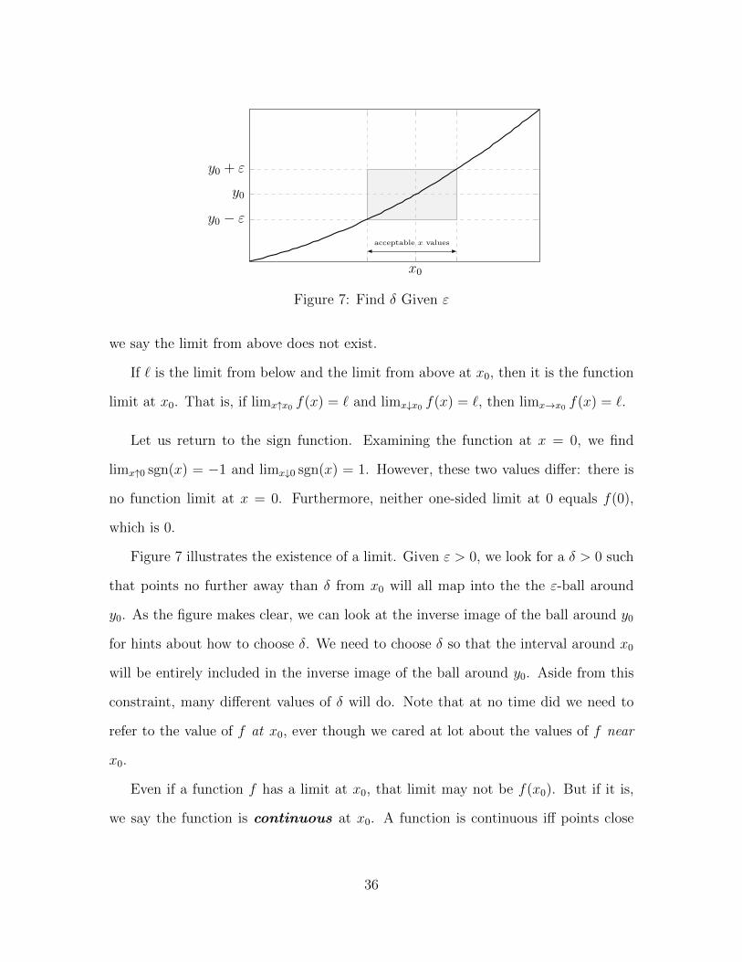
x0

y0 − εy0

y0 + ε

acceptable x values

Figure 7: Find δ Given ε

we say the limit from above does not exist.

If ` is the limit from below and the limit from above at x0, then it is the function

limit at x0. That is, if limx↑x0 f(x) = ` and limx↓x0 f(x) = `, then limx→x0 f(x) = `.

Let us return to the sign function. Examining the function at x = 0, we find

limx↑0 sgn(x) = −1 and limx↓0 sgn(x) = 1. However, these two values differ: there is

no function limit at x = 0. Furthermore, neither one-sided limit at 0 equals f(0),

which is 0.

Figure 7 illustrates the existence of a limit. Given ε > 0, we look for a δ > 0 such

that points no further away than δ from x0 will all map into the the ε-ball around

y0. As the figure makes clear, we can look at the inverse image of the ball around y0

for hints about how to choose δ. We need to choose δ so that the interval around x0

will be entirely included in the inverse image of the ball around y0. Aside from this

constraint, many different values of δ will do. Note that at no time did we need to

refer to the value of f at x0, ever though we cared at lot about the values of f near

x0.

Even if a function f has a limit at x0, that limit may not be f(x0). But if it is,

we say the function is continuous at x0. A function is continuous iff points close

36

together in the domain map to point close together in the range.13

Definition 5.3 (Continuity) a function f : X → Y is continuous at x iff limxt→x f(xt) =

f(x). (We can break this into two components: the function limit exists at x, and it

equals f(x).) A continuous function is continuous at each point in its domain.

A function may be continuous on a subset S of its domain, so that it is continuous

at every point in S. If f is a real function and f is continuous on the interval [a .. b],

we write f ∈ C[a, b].

A function is a continuous function on an interval (a .. b) iff it is continuous

at every point in (a .. b).

As a result, we find that for the illustrated value of ε, we cannot find a δ > 0 so

that f(B◦(0, δ)) ⊆ B(0, ε). No matter how small we make δ, the image includes −1

and 1, which are outside the ε-ball around y = 0. Once again, the value of f at 0 is

not important for the existence of a limit. Rather, it is important that the function

jumps at 0. As a result, the limiting value from the left (−1) differs from the limiting

value from the right (1).

A function f has the limit y0 at the point x0 if we can that ensure f(x) is as close

to y0 as we want just by ensuring that x is close enough to (but not equal to) x0.

We write this as f(x) → y0 as x → x0, and we say the y0 is the limit of f(x) as x

approaches x0. If it is not possible to provide such assurances, we way the limit of

f(x) does not exist at x0.

We formalize being close by desribing neighbhorhoods of these points. The core

concept is that given any neighborhood Ny0 of y0 we can find in the domain of f a

small enough punctured neighborhood N ◦x0

of x0 that its image f(N ◦x0

) is entirely

included in Ny0 .

13Continuity is given a more general treatment in the analysis chapter.

37

The neighborhood is around x0 is punctured : it does not include x0. Right now,

while developing the limit of a function, we want to ignore f(x0). But we will come

back to it in order to complete our discussion of continuity. For now just note that

f(x)→ y0 as x→ x0 does not imply that f(x0) = y0.

For real functions, we can use open intervals as our neighborhoods to illustrate this

idea. Recall from section 1.1.1 that an open interval (a .. b) comprises all the points

between a and b, not including the endpoints. Define an ε-radius interval around a

point y0 as follows: B(y0, ε) = (y0 − ε .. y0 + ε). This is just the set of points whose

distance from y0 is less than ε, which we can also write as {y | abs(y − y0) < ε}. We

will call this the ε-radius open ball around y0. If we exclude the center point, we

can produce a related punctured interval: B◦(x0, δ) = {x | 0 < abs(x − x0) < δ}.

This is the open set containing points no further than δ from x0, but not including

x0. Then we say y0 is the limit of f at x0 if for any ε > 0 we can always find a small

enough δ > 0 that the image of B◦(x0, δ) is included in B(y0, ε). For obvious reasons,

this is often known as the δ, ε-definition of the limit of a function.14

Again, f(x) → y0 as x → x0 does not imply that f(x0) = y0. It may even be

the case that f(x0) is not defined. Consider Figure 8. The function sin(x)/x is not

defined at x = 0. (We illustrate this in figure 8 by marking the “gap” in the function

with a dot.) Yet 1 is the limit of sin(x)/x as x approaches 0. This illustrates why we

work with punctured neighborhoods: we want a limit concept that does not depend

on the value of f(x0), or even that there be any such value.

For example, in figure 8, we can certainly ensure that the value of f remains in

(0.75 .. 1.25) by considering only x values in (−1.0 .. 1.0) (but not including 0). If we

insist that the value of f be in the narrower interval (0.95 .. 1.05), we need to choose

a smaller neighborhood of x, such as (−0.2 .. 0.2) (but not including 0).

14The δ, ε-definition extends to any metric space; see the analysis chapter for details.

38

-0.5

0

0.5

1

1.5

-5 0 5

ε =0.25

sin(x)/x

-0.5

0

0.5

1

1.5

-5 0 5

ε =0.25, δ=1

0.8

0.9

1

1.1

-1 0 1

ε =0.05

0.8

0.9

1

1.1

-1 0 1

ε =0.05, δ=0.2

Figure 8: Limit of sin(x)/x at x = 0

The same approach works with the function

f(x) =

sin(x)/x x 6= 0

0 x = 0

(18)

Now our function is defined at x = 0, but it has a “jump” there. Unless we work with

a punctured neighborhood, this jump would frustrate our attempt to find a δ to go

with our ε.

5.2 Limits and Continuity

Recall that a continuous function maps points near each other in the domain to

points near each other in the range. A function that is not continuous is called

discontinuous . A discontinuous function has some kind of jump and gap, such as

39

f(x0)

x0

f(x0)

x0

Figure 9: Continuous vs. Discontinuous at x0

we considered in the previous section.

When we do not face such gaps or jumps, we say our function is continuous. In

Figure 8, a discontinuity at 0 arose because sin(x)/x is undefined at 0. Defining a

new function by defining f(0) = 0 did not remove the discontinuity. The limit of the

function remains well defined, but the function is still not continuous at 0. However,

we can “plug” this discontinuity if we work with a very slightly different function:

f(x) =

sin(x)/x x 6= 0

1 x = 0

(19)

This plugs the “hole” in the graph, producing a continuous function. For ε = 0.25

and ε = 0.05, the figure illustrates choosing a δ that ensures we have only acceptable

x values in the δ interval around 0.

Figure 9 illustrates another type of “jump” that creates a discontinuity.

40

For any sequence (xn)n∈I in the domain of the function f , we can produce a corre-

sponding image sequence(f(xn)

)n∈I. Recall that an infinite sequence (xn) converges

to x if almost all of the elements are arbitrarily close to x.15 In this case we call x the

limit of the sequence and write xn → x. For a moment, consider only sequences that

converge to x but do not have x as an element. If for each such sequence the image

sequence has the limit y, we say that y is the sequential limit of f as x approaches

x. We often write f(x)→ y as x→ x, or even more compactly, limx→x f(x) = y.

Now consider all sequences that converge to x, even those that have x as an

element. If whenever xn → x it is also the case that f(xn) → f(x), we say the

function f is sequentially continuous at x. If a function is continuous at every

point in an interval, we say it is continuous on that interval. If a function is continuous

at every point in its domain, we say it is a continuous function. Roughly speaking,

you can draw a the graph of a continuous real function without lifting your pencil

from the paper.

We have seen that if f is a continuous function then f(x) must approach f(x) as x

approaches x. That is, we can push f(x) as close to f(x) as we wish by picking x close

enough to x. This is the idea behind the so-called “delta-epsilon” characterization

of continuity, which says that for each ε > 0 we can find some δ > 0 such that

|f(x+ dx)− f(x)| < ε as long as | dx| < δ.

5.3 Intermediate Value Theorem

The Intermediate Value Theorem is useful when thinking about the zeros of

continuous functions. The theorem says that a continuous function can transition

from one value to another only by passing through all the values between. This

is illustrated by Figure 10. To prove this theorem, we need to recall a math fact:

15By “almost all” we mean all but a finite number. See the analysis chapter for more detail.

41

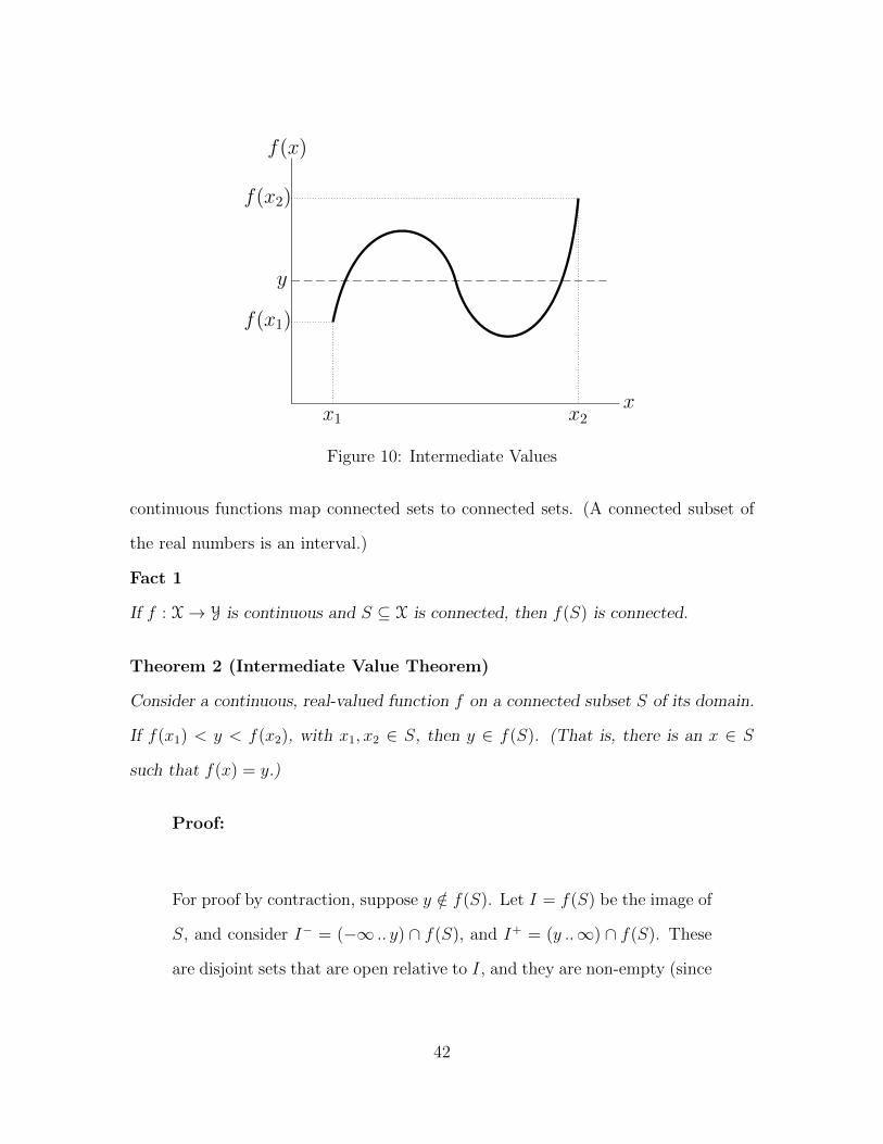
x

f(x)

x1 x2

f(x1)

f(x2)

y

Figure 10: Intermediate Values

continuous functions map connected sets to connected sets. (A connected subset of

the real numbers is an interval.)

Fact 1

If f : X→ Y is continuous and S ⊆ X is connected, then f(S) is connected.

Theorem 2 (Intermediate Value Theorem)

Consider a continuous, real-valued function f on a connected subset S of its domain.

If f(x1) < y < f(x2), with x1, x2 ∈ S, then y ∈ f(S). (That is, there is an x ∈ S

such that f(x) = y.)

Proof:

For proof by contraction, suppose y /∈ f(S). Let I = f(S) be the image of

S, and consider I− = (−∞ .. y) ∩ f(S), and I+ = (y ..∞) ∩ f(S). These

are disjoint sets that are open relative to I, and they are non-empty (since

42

f(x1) ∈ I− and f(x2) ∈ I+). The assumption that y /∈ f(S) implies that

I− ∪ I+ = f(S), so f(S) is not connected.

Therefore y ∈ f(S).

5.4 Functions with Zeros

In the sequence chapter we learn that a continuous function is one that maps points

that are close together in the domain to points that are close together in the range, so

that limxt→x f(xt) = f(x). A key attribute of continuous functions is f cannot pass

from one value to another without taking on all the values in between. This insight

is captured by the Intermediate Value Theorem, discussed in section 5.3.

The most common use of the Intermediate Value Theorem is to observe that the

a real-valued, continuous function must pass through zero if it changes sign over an

interval. (This version is sometimes called Bolzano’s Theorem .

43

Example 17

Let f(x) = x3. Note that f is continuous on the interval [−1 .. 1]. Since f(−1) < 0

and f(1) > 0, we know f has a zero in this interval. (Futhermore, since the function

is strictly increasing on this interval, there is only one.)

Let f(x) = lnx − 1. Note that f is continuous on the interval [2 .. 3]. Since

f(2) < 0 and f(3) > 0, we know f has a zero in this interval. (Futhermore, since the

function is strictly increasing on this interval, there is only one.)

Let f(x) = e−x − x, which is continuous on the interval [0 .. 1]. Since f(0) > 0

and f(1) < 0, we know f has a zero in this interval. (Futhermore, since the function

is strictly decreasing on this interval, there is only one.)

Let f(x) = −1 for x < 0 and f(x) = 1 for x ≥ 0. Note that f changes sign on

the interval [−1 .. 1], but it is discontinuous at 0. Due to the discontinuity we cannot

apply the IVT, and in fact f does not take on the value of 0.

If we can find a value x such that f(x) = 0, we say that x is a zero of f or a

root of the equation f(x) = 0. (It is also farily common to say the x is a root of f .)

There may be no real roots, a unique real root, or multiple real roots. There may

also be complex roots, but for now we focus on real roots.

Definition 5.4 Give a continuous function f : R → R, the basic root-finding

problem is to find x such that f(x) = 0.

Note that this problem is equivalent, for a continuous function g, to finding x such

that g(x) = k. (Just define f(x) = g(x)− k.)

Sometimes it is easy to find roots analytically. As a familiar example, we can solve

a0 + a1x = 0 for x = −a0/a1. As long as a1 6= 0, this will give use one real root. As

another example, we can solve a0+a1x+a2x2 = 0 for x = (−a1±

√a2

1 − 4a2a0)/(2a2).

As long as a21 > 4a2a0, this will give us two distinct real roots. In many other cases,

44

it may be impossible to find analytical expressions for the roots of an equation, and

we may turn to graphical and numerical techniques.

5.5 Finding Zeros by Exhaustive Search

If we know a continuous real function changes sign on an interval, we know it has a

zero in that interval. In principal, we can consider an arbitrary number of values in

the interval and pick the one with a function value closest to zero.

Here is a simplistic approach to exhaustive search. Our algorithm requires a

continuous function, an interval (xmin, xmax) bracketing the root, and a tolerance xtol

specifying the maximum acceptable deviation of the root we find from the true root.

Function exhaust iveFindMinimizer ( f , xmin , xmax , x t o l ) :

x ← xmin

xbest , f b e s t ← xmin , f ( xmin )

while x < xmax :

x ←↩+ x t o l

fx ← f ( x )

i f fx < f b e s t :

xbest , f b e s t ← x , fx

return xbest

Function exhaust iveFindRoot ( f , xmin , xmax , x t o l ) :

Function f2min ( x ) :

return abs ( f ( x ) )

return exhaust iveFindMinimizer ( f2min , xmin , xmax , x t o l )

One problem with exhaustive search is that it can be computationally expensive.

For example, suppose we are looking for the zero of f(x) = e−x−x. It is easy to verify

45

that this function changes sign on the interval [0 .. 1], since f(0) = 1 and f(1) < 0.

Futhermore, it is strictly decreasing. (See the dcalc chapter.) Therefore it has one

real zero, which is in the interval (0 .. 1). If we only need to be within 0.01 of the root,

exhaustive search will require 100 function evaluations. But if we need to be within

10−−6 of the root, it will require 106 function evaluations.

Suppose we are interesting in the zeros of a real function, f : R → R. It is

natural to begin by plotting the function. If we are thoughtful when we plot the

function, plotting may offer a quick way to learn how many real roots a function has

and approximately what their values are. Before plotting the function, we need to

decide on a portion of its domain over which to plot it. We need to be careful at this

point, or our plot may not reveal the zeros of the function. Although sometimes we

must resort to simple experimentation to choose our viewing window, often a quick

examination of the function often yields useful information.

Plotting x 7→ e−x − x over the interval [0 .. 1] yields Figure 11. On the one

hand, plotting works like our exhaustive search algorithm: plotting software will plot

(x, f(x)) for a limited number of values of x. On the other hand, Figure 11 suggests

a better way to refine our seach than evaluating more points on the entire interval.

It looks like our root is a little less than 0.6. We could refine our viewing window

to pin down the root more precisely, as in Figure 12. When we need more precise

characterizations of the roots of a function, we often turn to numerical methods that

make use of this kind of information about the function.

5.6 Root Approximation by Bracketing

In this section we introduce particularly simple numerical methods for approximating

a zero of a function. Our approach directly exploits the intermediate value theorem,

46

0 0.5 0.6 1−1

0

1

x

e−x−x

Figure 11: Root Approximation by Plotting

0.5 0.55 0.6

0

x

e−x−x

Figure 12: Root Approximation by Plotting (with Refinement)

47

which tells us that a continuous function has a zero on any sign changing interval.16

Take another look at our plot in Figure 11. We see that this continuous function

is positive at 0.5 and negative at 0.6. The intermediate value theorem tells us there

is a zero is between 0.5 and 0.6. We can therefore say the interval [0.5 .. 0.6] bounds

a real root. If that is enough precision for us, we can stop.

But we want more precision. So let us look at the value of the function in between

the two endpoints of our bounding interval. For example, consider the value of our

function at 0.55. If the value is positive, we know the root is greater than 0.55. (That

is, it surely falls in the interval [0.55 .. 0.6].) If the value is negative, we know the root

is less than 0.55. (That is, it surely falls in the interval [0.5 .. 0.55].) Either way, we

have confined the root to a smaller interval.

In this case, Figure 12 shows that by enlarging our viewing window we can see

that the function value is positive a x = 0.55. Thus we would replace the lower

endpoint (0.5) with the new value (0.55), but we retain the upper endpoint of 0.60.

This gives us a new, narrower interval of (0.55 .. 0.60), while ensuring that a zero of

our continuous function is still bracketed. We have increased the precision with which

we know the root.

This is an approach we could repeat over an over again. Each time we try a

new point, we get to shrink our interval, either by moving the left boundary or the

right boundary of the interval. Listing 3 summarizes an iterative process that uses

this logic repeatedly to shrink the bracket around the root. The listing assumes we

have access to two helper functions. The reiter function returns True as long as we

want an additional iteration. The nextpoint function provides us with a point in the

interval.

16In fact one algoritm we present embodies a common proof of the intermediate value theorem.See for example (Edwards, 1973, p.446).

48

Listing 3: Approximate Root via Bracketing

Function bracket (f : Callable , #f l o a t→ f l o a t ( c o n t i n u o u s f u n c t i o n )

xa (float), #i n t e r v a l l o w e r bound

xb (float), #i n t e r v a l uppe r bound

nextpo int : Callable , #( f l o a t , f l o a t , f l o a t , f l o a t )→ ( f l o a t , f l o a t )

r e i t e r : Callable , #( f l o a t , f l o a t , f l o a t , f l o a t , i n t )→ b o o l

) → f loat : #x ∈ ( xa . . x b ) s . t . f ( x ) ≈ 0

fa , fb ← f ( xa ) , f ( xb )ct ← 0while r e i t e r ( xa , xb , fa , fb , c t ) :

xnew ← nextpo int ( xa , xb , fa , fb )fnew ← f ( xnew)i f ( fnew · f a > 0) then:

xa , f a ← xnew , fnewotherwise:

xb , fb ← xnew , fnewct ← ct + 1

return xa i f (abs ( f a ) < abs ( fb ) ) else xb

Listing 4: Bisect Sign-Changing Interval

Function xmid ( xa , xb , fa , fb ) :return ( xa + xb )/2 .0

How are we going to choose our next point each iteration? We can imagine a

variety of approaches. We could simply choose a random point in the interval. Or,

as we did above, we could split the interval in half each time. The algorithm that

results from always picking the midpoint of the interval as our next point is know,

naturally enough, as the bisection algorithm for root finding. Listing 4 illstrates

this approach to producing the next point. (The bisect function depends only on

the values in the domain and does not use other information, but it accepts two more

arguments so that it can serve as our nextpoint function.)

Our bracketing algorithm can use our interval-bisection function to produce the

49

Listing 5: Convergence Criteria: ftol

Function f t o l ( xa , xb , fa , fb , i t r ) :f t o l ← 1e−9return (abs ( f a ) > f t o l ) and (abs ( fb ) > f t o l )

core of a bisection algorithm. For the next point, we find the midpoint of the current

interval. We use this new point as one endpoint for a new interval; for the other

endpoint, we retain one of the previous points. We do this in a way that ensures that

we still have a sign-changing interval. This produces a sign changing interval half as

wide as the one we started with.

If we adopt the midpoint of the interval as our root approximation, our error will

be less than half the width of the interval. If we want an even more accuracy, we

can repeat the bisection process as many times as we wish. Each time we bisect the

bounding interval, we more narrowly bound the root. Proceding this we until we

are satisfied with the implied accuracy is known as the interval bisection method.

But, when should we be satisfied? There is no single answer to this question, but to

complete the algorithm, we must state our criterion explicitly. Listing 5 offers one

particularly simple approach: we are satisfied when the function value is close enough

to 0. (For illustration, here we simply hard-code the meaning of ‘close enough’.)

One we have a way to produce a new point in the current interval and a criterion for

when to stop doing this, we have complete specification of a bracketing root finder.

Listing 6 illustrates this, producing a bisection algorithm. This interval bisection

method is very reliable, and it uses very little information about the function.

Unfortunately, root finding by interval bisection can be rather slow to converge. If

we use information about the slope of the function, we may be able to greatly speed

50

Listing 6: Interval-Bisection Root Finder

Function b i s e c t i o n ( f , xa , xb ) :return bracket (

f , xa , xb ,nextpo int ← xmid ,r e i t e r ← f t o l )

Listing 7: Regula-Falsi Root Finder

Function x f a l s e ( xa , xb , fa , fb ) :lam ← fb/ ( fb - f a )return lam · xa + (1 - lam ) · xb

Function f a l s e p o s i t i o n ( f , xa , xb ) :return bracket (

f , xa , xb ,nextpo int ← x f a l s e ,r e i t e r ← f t o l )

up convergence. This is the approach taken by Newton’s method, which we explore

in section ??.

Computational Exercise 1

Modify the bisection algorithm of this section to test whether the initial interval spec-

ified by the user is sign-changing, as required by the algorithm. Raise an informative

error if it is not.

Further modify the algorithm to specially handle the (unlikely) case where the

image of the midpoint is exactly 0.

5.6.1 Linear Interpolation

The bisection method uses no information about the function other than its continuity

and its sign change on the interval. Given two points a and b that bracket a sign

changing interval, the bisection method always picks 0.5a + 0.5b as its new point to

51

test. The new point will stay in the interval, since it is simply an average the two

endpoints. Of course, any other method of averaging the endpoints will also produce

a point in the interval. In particular, a convex combination of the points will also

belong to the interval.

Of course, any convex combination of the points, λa+ (1− λ)b where 0 < λ < 1,

will produce a new point in the interval. The linear interpolation method chooses

λ by using limited information about the function: its values at its endpoints. (This

method is also known as the false position method or regula falsi method. A false

position is just an initial “wrong” guess: the approximate zero found by interpolation.)

Once again our object is to find a zero of a continuous function f in the interval

[a .. b], given f(a)f(b) < 0. This time we produce our new point in the interval by

linear interpolation between (xa, fa) and (xb, fb).

xnew = λa+ (1− λ)b

where λ =f(b)

f(b)− f(a)

(20)

Note that 0 < λ < 1, because we start with a sign-changing interval. It is somewhat

more common to see this expressed as

xnew =f(b)a− f(a)b

f(b)− f(a)(21)

This method is referred to as linear interpolation because x is the zero of the

52

Listing 8: Linear Interpolation Method

Function x f a l s e ( xa , xb , fa , fb ) :lam ← fb/ ( fb - f a )return lam · xa + (1 - lam ) · xb

Function f a l s e p o s i t i o n ( f , xa , xb ) :return bracket (

f , xa , xb ,nextpo int ← x f a l s e ,r e i t e r ← f t o l )

secant line through (a, f(a)) and (b, f(b)). That is,

xnew = a+ (1− λ)(b− a)

= a+−f(a)

f(b)− f(a)(b− a)

= a− f(a)(b− a)

f(b)− f(a)

(22)

To turn this into an iterative method, we test the sign of f at the new point, in

order to again produce a sign-changing interval. Since the true the solution remains

bracketed at each step, convergence is again guaranteed. However the width of the

bracket does not tend to zero: instead one end eventually remains fixed while the

other moves toward the root.

6 Concave and Convex Functions

When economists discuss the utility of wealth, they usually assume that successive

increments to a person’s wealth add less and less to utility. This declining marginal

utility of wealth implies that utility is a concave function of wealth. When economists

consider the costs of changing the capital stock, they usually assume that in any

53

x

f(x)

x

f(x)

x

f(x)

Figure 13: Concave Functions

period, successive increments to the capital stock cost more and more to put into

place in any given period of time. This these increasing marginal adjustment costs

imply that adjustment cost is a convex function of investment. Convex and concave

functions are in wide use in economics.

Consider a real function. We say this function is concave iff every secant segment

for the function lies (weakly) below the graph of the function. If every secant segment

lies strictly below the graph (except at its endpoints, of course), we say the function

is strictly concave.

The definition of convexity simply reverses the relationships above. So we say f

is convex iff every secant segment for the function lies (weakly) above the graph of f ,

and we say f is strictly convex iff every secant segment lies strictly above the graph

(except at its endpoints). Since a secant segment comprises the convex combinations

of two points of f , we can state these defintions as follows.17

Definition 6.1 (Concavity and Convexity) Consider a real-valued function f and

let X be a convex subset of its domain. We say f is concave on X iff for any

17Some authors use the terms ‘concave down’ for concave functions and ‘concave up’ for convexfunctions.

54

x

f(x)

x

f(x)

x

f(x)

Figure 14: Convex Functions

λ ∈ [0 .. 1] and for any two points x and x′ in X we have

f [λx + (1− λ)x′] ≥ λf(x) + (1− λ)f(x′)

We say f is strictly concave if for any λ ∈ (0, 1) and for any two distinct points x

and x′

f [λx + (1− λ)x′] > λf(x) + (1− λ)f(x′)

A function f is convex iff −f is concave. A function f is strictly convex iff −f is

strictly concave.

Exercise 8

Give a mathematical definition of a convex function, analogous to our definition of

concave function in definition 6.1.

Exercise 9

Use definition 6.1 to show that f is concave iff

f [x + (1− λ)(x′ − x)]− f(x) ≥ (1− λ)[f(x′)− f(x)]

Interpret this graphically.

55

Affine Functions A function that is both convex and concave is called affine .

Definition 6.2 (Affine Function) An affine function maps affine combinations of

points to affine combinations of their images. That is, f : X → Y is an affine function

iff for any scalar λ we have f [λx + (1− λ)x′] = λf(x) + (1− λ)f(x′).

A special case arises when the graph of an affine function passes through the

origin: such functions are called linear . The function f is linear if the value f(x) is

directly proportional to the value of x.

An affine function f : R→ R has a constant slope, so its graph is a straight line.

Based on the discussion so far, it seems natural to say that the slope of a concave

function is decreasing. Similarly, we would like to say the slope of a convex function

is increasing. We make this statement in terms of the difference quotient: at any

point, the backward differences are larger than the forward differences.

56

Theorem 3

Suppose the function R f→ R is concave on an interval, and that x0 − h1 and x0 + h2

are points in this interval, with h1, h2 > 0.

f(x0 − h1)− f(x0)

−h1

≥ f(x0 + h2)− f(x0)

h2

In other words, a concave function has a decreasing slope, as measured by the differ-

ence quotient. If f is strictly concave, then the inequality above is strict.

Proof:

We begin by defining x1 = x0 − h1, x2 = x0 + h2, and λ = h1/(h1 + h2).

This implies that 0 < λ < 1 and that x0 = λx2 + (1− λ)x1. By definition

of concavity,

f(x0) ≥ λf(x2) + (1− λ)f(x1)

so we have

0 ≥ λ[f(x2)− f(x0)] + (1− λ)[f(x1)− f(x0)]

or

−(1− λ)[f(x1)− f(x0] ≥ λ[f(x2)− f(x0]

Multiplying both sides by (h1 + h2)/h1h2, which is positive, and recalling

the definitions of λ, x1, and x2, we have

f(x0 − h1)− f(x0)

−h1

≥ f(x0 + h2)− f(x0)

h2

Q.E.D.

57

6.1 Jensen’s Inequality

We turn now to an alternative characterization of concavity that has proved useful

in many applications. We will refer to this as Jensen’s inequality.18

18The standard reference is Jensen (1906). See McShane (1937) and Beckenbach (1946) for dis-cussion, alternative approaches to proof, and some early generalizations.

58

Theorem 4

Let the function f : R → R be concave on the real interval [a .. b].19 Let x1, . . . ,xN

be points in the interval, and consider positive weights λ1, . . . , λN which sum to unity.

Construct the convex combinations∑λixi and

∑λif(xi). In this case, Jensen’s

inequality states that f at the weighted average of the points is larger than the

weighted average of the f values:

f(∑

λixi

)≥∑

λif(xi)

Proof:

Note that for N > 1,

N∑

i=1

λixi = λNxN + (1− λN)N−1∑

i=1

λi1− λN

xi

which is a convex combination of two points (with weights λN and (1 −

λN)). Concavity of f therefore implies the following inequality:

f

(N∑

i=1

λixi

)≥ λNf(xN) + (1− λN)f

(N−1∑

i=1

λi1− λN

xi

)

Since 1 − λN =∑N−1

i=1 λi, we can say that if Jensen’s equality holds for

N − 1 weights, then it also holds for N weights. Since it obviously holds

for a single weight, we can say (by induction) that it holds for any number

of weights. (See section ?? for a discussion of induction.)

19More generally, we can simply require that X be a closed and convex set.

59

Example 18

Apply Jensen’s inequality to the case of two weights:

f(λ1x1 + λ2x2) ≥ λ1f(x1) + λ2f(x2)

Note that λ1 = 1− λ2, so we have

f(λ2x2 + (1− λ2)x1) ≥ λ2f(x2) + (1− λ2)f(x1)

This inequality is directly implied by the concavity of f .

Example 19

As a standard illustration of Jensen’s inequality, we can compare two concepts of the

“average” of N positive real numbers, x1, . . . , xN . (Figure 15, based on Nelsen (1993,p.50), illustrates this relationship for two numbers.) We define the arithmetic meanas the sum of the number divided by N , and the geometric mean by the N -th rootof the product of the numbers.

meana =x1 + x2 + · · ·+ xN

Nmeang = (x1x2 . . . xN)1/N

Jensen’s equality implies that the log of the arithmetic mean is greater than the logof the geometric mean:

ln

(x1 + · · ·+ xN

N

)≥ 1

N(lnx1 + · · ·+ lnxN)

Since the logarithm is strictly increasing, the arithmetic mean will be weakly greaterthan the geometric mean. Indeed, since the logarithm is strictly concave, the arith-metic mean will be strictly greater than the geometric mean, whenever the xi are notall identical.

Exercise 10

Can Jensen’s inequality, as presented in theorem 4, be written as a strict inequality

if the function is strictly concave?

60

a

b

b a

(a+ b)2 > 4ab therefore (a+ b)/2 >√ab

Figure 15: Arithmetic Mean vs. Geometric Mean

7 Extrema

Some functions have extrema: a maximum or a minimum value reached by the func-

tion. Economists are often interested in locating such extrema, such as minimum

cost, maximum profits, or maximum utility.

Definition 7.1 (Extreme Point) Consider a set S in the domain of the function

f , and suppose there is a point x ∈ S where f achieves a value at least as great as

everywhere else in S. That value is called the maximum of f in S, and any point x ∈ S

where f achieves its maximum in S is called a maximizer of f in S.20 Similarly,

any point x ∈ S where f achieves a minimum in S is called a minimizer of f in S.

If x is a maximizer or a minimizer of f in S, we call x an extreme point of f in S,

and we say that in the set S the function f has an extremum at the point x.

Summarizing, an extreme point of f in the set S is a maximizer or a minimizer of

f in S. If f(x) ≥ f(x) for all x ∈ S, then x is a maximizer of f in S. If f(x) ≤ f(x)

for all x ∈ S, then x is a minimizer of f in S.

If a point x in the domain is a maximizer of f in the entire domain, we call x a

20Some authors refer to x as a “maximum” of f , which is a misleading terminology, or as amaximum point of f .

61

global maximizer of f , and we call f(x) a global maximum. (Some authors prefer

the term absolute maximum.) So if X is the domain of f , then a point x ∈ X is a

global maximizer iff f(x) ≥ f(x) for all x ∈ X.

At times we are also interested whether a point x is a maximizer relative to nearby

points. Let Nx be some “neighborhood” of the point x, and suppose x is a maximizer

of f in Nx. Then we call x a local maximizer of f . (An alternative term is ‘relative

maximizer’.) So roughly speaking, x is a local maximizer of f if we cannot find a

point near x that yields a bigger value of f . If a point is a local maximizer or a local

minimizer of f , we call it a local extremum of f . Clearly any global maximizer is also

a local maximizer.

Some functions have a unique maximizer. Suppose x is a global maximizer of f

on a set S, and that f(x) > f(x) for all other x ∈ S. Then we say that x is a strict

global maximizer of f in S. If x is a strict global maximizer of f on a neighborhood

of x, we say that x is a strict local maximizer of f . Our vocabulary for minimizers is

symmetric.

A natural question about a function is whether it reaches a maximum or minimum

value. This is addressed by the extreme value theorem.

62

Theorem 5 (Weierstrass Extreme Value Theorem)

Suppose a real-valued continuous function f is defined on a compact set S. Then f

attains a maximum value and a minimum value on S.

Example application: a utility function attains a maximum on a budget set.

Proof:

We will show that f has a maximum on S. (The proof for a minimum

is analogous.) To prove this we need to recall a couple math facts: (i) a

continuous function maps compact sets to compact sets, and (ii) a set of

real numbers is compact iff it is closed and bounded. From (i) we know

f(S) is compact, and therefore from (ii) that it is closed and bounded.

Let ymax be the least upper bound of f(S). Now f(S) contains its least

upper bound since it is closed, therefore there is a maximizer xmax such

that f(xmax) = ymax.

Exercise 11

Consider the function f(x) = x2: does it attain a maximum and a minimum on the

open interval (−1, 1)? Consider the function g(x) = x−2 for x 6= 0 with g(0) = 1:

does it attain a maximum and a minimum on the closed interval [−1 .. 1]? In each

case, determine whether the conditions of the Extreme Value Theorem are met.

7.0.1 Optimization

Sometimes we use the notation

x ∈ arg maxx∈S

f(x) (23)

63

That is, x is a value of the argument x that solves the maximization problem

maxx∈S

f(x) (24)

In economics our interest in extrema emerges quite naturally. Generally we char-

acterize economic actors by an objective function, a goal (to maximize or minimize

the objective function), and a constrained set of choice variables. The objective func-

tion may be a utility function, cost function, or profit function. The choice variables

may be quantities of goods to consume or quantities of inputs into a production pro-

cess. The goal is to reach an extreme value of the objective function subject to any

constraints. If we are given an objective function f(x) to maximize, we would like

to choose x to make the value of f as large as possible. For example, a consumer

is characterized by a utility function, choice variables that include the quantity of

various goods to consume (subject to a budget constraint), and the goal of maximiz-

ing the value of the utility function by selecting the optimum quantities of various

consumption goods.

Once we have an objective function and a goal, we can characterize an optimization

very generally. For example, a maximization problem can be characterized as

maxx∈S

f(x, θ) (25)

where f depends on our choice variable (x) and perhaps other factors θ, and our

choice must be made from the set S.

Algorithmic Optimization Conceptually, the problem is in some sense trivial.

We just need to check the value of f for each x ∈ S. If S is finite, we can in principle

approach this algorithmically. Given any x0 ∈ S, we might implement the following

64

algorithm.

xbest , fmax ← x0 , f ( x0 )for x ∈ S :

f t e s t ← f ( x )i f f t e s t > fmax :

xbest , fmax ← x , f t e s t

Given enough time to consider every element, this algorithm will find a maximizer

and the associated value of f . Of course, if S is infinite (or even very large) we cannot

literally check each value. In later chapters, we will consider this problem in detail.

Graphs as Aids to Optimization Graphs can serve as aids to optimization. Here

we consider a simple example of choice of technique. Suppose you are trying to decide

which of several techniques is best for some activity. Each technique produces costs

and benefits dependent on the level of the activity, as measured by a real number. You

can simply plot this dependence over the relevant range of the activity, and choose

the technique that yields the largest net benefits.

A

B

C

E

D

x

f(x)

Figure 16: Extrema: Local and Global

65

Theorem 6 (Slope Test)

Let f be a real-valued function of a real variable and S be some subset of the domain.

Then x is a maximizer of f in S iff each forward difference at x is nonpositive and

each backward difference at x is nonnegative. Similarly, x is a strict maximizer of f

in S iff each forward difference in S at x is negative and each backward difference in

S at x is positive.

Proof:

Suppose x is a strict maximizer of f in S. Then at any other available

point we must have a smaller value for f . That is, x ∈ S implies f(x) −

f(x) < 0. For x 6= x define h = x− x, and write the associated difference

quotient at x:

q(x, h)def=

f(x+ h)− f(x)

h

The numerator is always negative, and the denominator has the sign of h.

For x 6= x in S, define h = x− x. Suppose h > 0 =⇒ q(x, h) < 0. Then

h > 0 =⇒ f(x + h) < f(x). Similarly, suppose h < 0 =⇒ q(x, h) > 0.

Then h < 0 =⇒ f(x + h) < f(x). So if the difference quotient at x

always has the oppositive sign as h, then x is a strict maximizer of f on

S.

The proofs for a nonstrict maximizer are similar.

Similarly, if x is a minimum, then the difference quotients at x share the sign of h.

66

Example 20

Consider the function defined by the rule f(x) = |x| and the point x = 0. Given any

x, define h = x− x. We have the associated difference quotient

q(0, h)def=|x+ h| − |x|

h=|h|h

If h > 0 then |h| = h so that q(0, h) = 1. If h < 0 then |h| = −h so that q(0, h) = −1.

A difference quotient at 0 will therefore always share the sign of h, implying that 0

is a strict global minimizer of |x|.

7.0.2 Inflections

A function may be concave in some parts of its domain and convex in other parts.

Where it is strictly concave, the function is said to have negative curvature. Where it

is strictly convex, the function is said to have positive curvature. Where the curvature

changes sign, the function is said to have an inflection point.

Consider a real-valued function f on an interval (a, b). We say that x ∈ (a, b)

is an inflection point of f if the curvature of f changes sign at x. For example, if

f has negative curvature over (a, x) and positive curvature over (x, b), then x is an

inflection point of f .

Problems for ReviewExercise 12

Theorem 1 tells us that a function f is strictly increasing if its difference quotient is

always positive. Similarly, f is strictly decreasing if its difference quotient is always

negative. Calculate the difference quotient for each of the following functions. (Use

the arbitrary points (x0, f(x0)) and (x0+h, f(x0+h)).) Use the value of the difference

67

quotient to determine whether or not the function is monotone, and explain your

reasoning in each case.

f(x) = 3x+ 5

f(x) = −2x+ 5

f(x) = x2

f(x) = x3

Exercise 13

In example 10 we introduced the cost function

TC = 100 + 20Q

What is the natural domain for this cost function? What is the economic domain for

this cost function? Suppose this is the cost function of a firm that has a capacity

constraint: it cannot produce more than 1000 units of output. In this case, what is

the economic domain for this cost function?

Exercise 14

Which of the following functions are injections (i.e., one-to-one)? Which of the fol-

lowing functions are surjections (i.e., onto)?

� a function mapping high school graduates to the high school graduated from

� a function mapping Dewey decimal classifications to book titles

� a function mapping Nobel prize winning economists to the year of their prize

Exercise 15

Which of the following functions have inverses?

68

� f : Z+ → Z where f(x) = x2

� f : R→ R where f(x) = x2

� f : R→ R where f(x) = 3√x

In each case, explain your answer.

Exercise 16

Given the parameters m and b, the graph of the real-valued function defined by

f(x) = mx + b is a straight line. Such a function is called affine, although we often

loosely call it linear. Use the difference quotient to explain why any such function is

monotone. Also, determine whether such an affine function is concave or convex.

Exercise 17

Let f : R→ R be a concave function. Prove that for any λ ∈ [0, 1) and x′ > x,

f(x+ (1− λ)(x′ − x)

)− f(x)

(1− λ)(x′ − x)≥ f(x′)− f(x)

x′ − x

Exercise 18

Suppose the function R f→ R is concave on an interval, and x0 < x′ < x1 are three

points in this interval. Show that

f(x′)− f(x0)

x′ − x0

≥ f(x1)− f(x0)

x1 − x0

If f is strictly concave, show that the inequality above is strict.

Exercise 19

A function that satisfies f(x + x′) ≤ f(x) + f(x′) is called subadditive . Show that

if f : R+ → R+ is concave, then it is subadditive. Note that the same technique can

be used to show that if f : RN+ → RN

+ is concave, then it is subadditive along any ray

through the origin.

69

Exercise 20

Give a verbal description of each of the following families of functions. Be sure to

state the natural domain in each case.

� f(x) = xn where n is a positive, even integer.

� f(x) = xn where n is a positive, odd integer.

� f(x) = xn where n is a negative, even integer.

� f(x) = xn where n is a negative, odd integer.

� f(x) = x1/n where n is a positive, even integer.

� f(x) = x1/n where n is a positive, odd integer.

Exercise 21

The Bank of Sweden Prize in Economic Sciences in Memory of Alfred Nobel was

instituted in 1968, at the tercentenary of the bank. This is popularly known as the

Nobel Prize in Economics. The Nobel Foundation maintains a list of the laureates

at http://www.nobel.se/economics/laureates/. The list is updated annually in

mid-October, upon the announcement of the new laureate(s). Call the set of dates

D. Call the set of last names L. Can you construct a function from D to L? If so,

do it. Can you construct a function from L to D? If so, do it.

Exercise 22

Let n ∈ N∗. Prove that f : R → R has the homogeneity property f(λx) ≡

λnf(x) ∀λ ∈ R iff f(x) = f(1)xn.

Exercise 23

Consider a function f : R → R that has been transformed as follows: g(x) =

ay + byf(ax + bxx). Suppose you know that f(x0) = 0. What value of g does that

determine?

70

Exercise 24

Suppose we define the adjustment cost function c = x2 on the domain {x | −2 ≤ x ≤

2}. What is the range of the function?

Computational Exercises

Computational Exercise 2

Implement the consumption function in Listing 1. Enforce the domain restriction

that yd ≥ 0.

Computational Exercise 3

Define two functions f(x) = x2 and g(x) =√x, and then define the composition

f ◦ g(x) = f(g(x)). What happens if you provide a negative argument to your func-

tion fog? Explain.

Computational Exercise 4

Implement the pseudocode in Listing ?? to define a function qfxh(f,x,h) that com-

putes a difference quotient from x to x+ h for the function f . Use it to compute the

difference quotient when f(x) = x2 and x = −1, letting h take on the three values

1, 2, 3. Add a program comment explaining your results.

Computational Exercise 5

Write a function or procedure that implements the interval bisection algorithm in

listing 4. Your input arugments must include a function and two real numbers, which

must bound a sign changing interval. Feel free to improve on listing 4, perhaps by

eliminating unnecessary function evaluations.

Computational Exercise 6

Use the polynomial evaluation procedure you created in exercise ?? to determine the

decimal value of the binary number 1100111. [Hint: what does each digit in this

binary number represent?]

71

Computational Exercise 7

Write a procedure to compute multiple values of a polynomial as follows. Your

procedure should have two input arguments: a vector of polynomial coefficients and

a vector of values of the independent variable. Your procedure should return a vector

containing the evaluation of the polynomial at each value input for the independent

variable. Use this procedure to graph the polynomial f(x) = 3 − 2x − x2. (Hint:

evaluate all points at the same time using element-by-element multiplication.)

Recommended Reading

Simon and Blume (1994, ch.2); Carter (2001, ch.2.1); Klein (2001, ch.2); Chiang

(1984, ch.2,3); Velleman (2006, ch.5); de la Fuente (1999, 1.1); McShane (1937).

Bibliography

Beckenbach, E. F. (1946, November). “An Inequality of Jensen.” The American

Mathematical Monthly 53(9), 501–505.

Carter, Michael (2001). Foundations of Mathematical Economics. Cambridge, MA:

MIT Press.

Chiang, Alpha C. (1984). Fundamental Methods of Mathematical Economics (3rd

ed.). New York: McGraw-Hill, Inc.

de la Fuente, Angel (1999). Mathematical Methods and Models for Economists. Cam-

bridge, UK: Cambridge University Press.

Edwards, Jr., Charles Henry (1973). Advanced Calculus of Several Variables. New

York: Academic Press.

72

Jensen, Johan Ludwig William Valdemar (1906). “Sur les Fonctions Convexes et les

Inegalites entre les Valeurs Moyennes.” Acta Mathematica 30, 175–193.

Klein, Michael W. (2001). Mathematical Methods for Economics (2nd ed.). Boston,

MA: Addison-Wesley.

McShane, E. J. (1937, August). “Jensen’s Inequality.” Bulletin of the American

Mathematical Society 43(8), 521–527.

Nelsen, Roger B. (1993). Proofs without Words: Exercises in Visual Thinking. The

Mathematical Association of America.

Simon, Carl P. and Lawrence Blume (1994). Mathematics for Economists. New York:

W.W. Norton & Company, Inc.

Strachey, Christopher (2000). “Fundamental Concepts in Programming Languages.”

Higher-Order and Symbolic Computation 13, 11–49.

Velleman, Daniel J. (2006). How to Prove It: A Structured Approach (2nd ed.).

Cambridge, UK: Cambridge University Press.

Appendix: Computing Monomials

Suppose we wish to compute the value xn for some postive integer n. The most

obvious way to do this is to multiply x times itself n times. Recall that the repetition

of a computational process over and over again is called iteration . In this section

we will illustrate how to compute the value of a monomial using iteration.

73

Listing 9: Compute Monomial: Recursive

#g o a l : r e c u r s i v e c ompu t a t i o n o f xˆn

#i n p u t :

# x : number

# n : n o n n e g a t i v e i n t e g e r

#o u t p u t :

# xˆn

Function monomial2 (x , n) :i f (n > 0) then:

#compute xn w i t h r e c u r s i v e f u n c t i o n c a l l

xn ← x ·monomial2 (x , n−1)otherwise:

#compute b a s e c a s e

xn ← 1return xn

7.1 Computing Monomials Recursively

We will briefly explore a recursive approach to computing the value of a monomial.

This relies on our recursive definition of the value of a monomial in (16).

When our code uses a function to compute a specific value, we will say that the

code contains a call to the function. A function is said to be recursive if its defintion

contains a call to itself. Recursive functions may prove useful when a computation

can be broken into identical processing steps involving changing data. A recursion

would go on forever if not for the base case. The base case is computed without

recursion. When the base case is reached, the recursion ends.

In listing 9, each time the function is called we test to see if n > 0. If this criterion

is met, we compute xn−1 recursively and produce xn = xxn−1. Otherwise our base

case applies: we then return the invariant value 1 rather than recursively calling the

function.

Note that we cannot return from the first function call until its recursive call

74

returns, which means that every recursive function call “stacks up” until the end test

is met. This “stacking up” of the function calls, along with the variables local to each

function call, means that deep recursion can be computationally expensive. To avoid

this expense, we often try to write equivalent iterative algorithms. An iterative

algorithm does repetitive recalculation without recursion.

7.2 Divide and Conquer

So far we have considered two straightforward ways to compute the value of a mono-

mial. It turns out however that these straightforward algorithms are also very waste-

ful. This wastefulness is not very costly if x and n are small integers, but in many

econometric applications it can matter a great deal.21 To illustrate the wastefulness,

consider the 64 multiplications that our first two algorithms required to compute x64.

We could compute x64 = x32x32 and save about half of these multiplications, and we

could compute x32 = x16x16 and save about half of the remaining multiplications, and

so on until we get down to x0 (which we know to be 1). This observation suggests a

“divide and conquer” algorithm to compute xn.

Of course computing x64 was particularly simple: we can start with x and just

keep squaring it, because 64 is a power of 2. But the basic idea can be adapted, as

in listing 10.

Given values for x and for n, we begin by initalizing two values: xn=1 and sq=x.

The iterative process is implemented in a while loop. As long as n > 0, the loop

will keep executing. (Zero is equivalent to False and nonzero values are True.) At

each iteration we set sq=sq*sq and n=n//2. However we only update xn when n is

currently odd, in which case we set xn=xn*sq.

21For example, we may need to compute powers of a large square matrix.

75

Listing 10: Compute Monomial: Divide and Conquer

#g o a l : c ompu t a t i o n o f xˆn by d i v i d e and con qu e r

#i n p u t :

# x : number

# n : n o n n e g a t i v e i n t e g e r

#o u t p u t :

# xˆn

Function monomial3 (x , n) :xn ← 1sq ← xwhile (n) :

i f (n%2) then:xn ← xn · sq

n ← n//2i f (n) then:

sq ← sq · sqreturn xn

This means that we consider xn as a product of powers of x, where all the expo-

nents are powers of 2.22 For example, x25 = x1x8x16. We use an extra variable (sq)

to accumlate x1, x2, x4, . . . as we iterate. So by working through the algorithm, we

compute x25 as follows:

n 25 12 6 3 1 0

sq x1 x2 x4 x8 x16

n%2 1 0 0 1 1

xn 1 x1 x1 x1 x9 x25

Inside the loop we break n/2 into two parts.23 The // operator is called the floor-

division operator, and the % operator is called the modulo operator (or remainder

22We effectively work with the binary representation of n. Note the role of the binary representa-tion: 2510 = 110012, which we can read in reverse order in the third row of the table.

23The notation for floor division varies across languages. Many languages do not have a floordivision operator, but many have the floor function, and you can compute a floor division asfloor(n/2). In Python you can compute both the quotient and remainder with the divmod builtinfunction.

76

operator). The value n//2 is sometimes called the “floor division” of n by 2; it returns

the largest integer less than n/2. (Sometimes we call n // 2 the quotient of n/2.) The

remainder n%2 is 0 if n is even and 1 if n is odd.

So if n is odd, we multiply xn by sq and assign the result to xn. We will find

n//2 > 0 only if n > 1, so if n > 1 we square sq. This is simply stored for the next

interation. Note that we assigned n//2 to n, so at each iteration is cut roughly in

half. This ensures that n will eventually be zero, and we will exit the loop.

Computational Exercise 8

Implement the “divide and conquer” algorithm in listing 10. (If you are comfortable

with matrices, write your function so that it can also compute powers of an arbitrary

square matrix.) Your code should basically follow the intuition we provided for the

divide and conquer strategy, but you must considers an important detail: at each

iteration, be sure to consider the possibility that n is odd.

Computational Exercise 9

Construct an recursive version of the recursive “divide and conquer” algorithm in

listing 10. (If you are comfortable with matrices, write your function so that it can

also compute powers of an arbitrary square matrix.) Be sure to considers an important

detail: each time your recursive function is called, consider the possibility that n is

odd. If n is even, compute xn = xn/2xn/2. If n is odd, compute xn = xxn//2xn//2.

77

Vectors

82

Economists encounter vectors in economic theory, econometric theory, and econo-

metric applications. Two core reasons for this ubiquity are notational compactness

and computational convenience. In the present chapter, we will learn enough about

vectors to undertake some economic applications.

1 Introduction to Vectors

A real tuple is a finite array of real numbers. These numbers are called the elements

(or components , or coordinates) of the tuple. We call a tuple with N elements

an N -tuple, and we sometimes loosely say that it is N -dimensional. The number

of elements N is called the length or size of the tuple. For example, (0, 1) is a

real 2-tuple, and (0, 1, 2) is a real 3-tuple. The left-most element is called the first

coordinate. Two tuples are equal if they are equal element-wise. This means that

order matters: (0, 1) and (1, 0) are two different tuples.

Tuples become vectors when we provide rules for adding them and scaling them.

(We will characterize these rules in the next section.) The symbol RN denotes the

set of all real N -vectors. For example, (0, 1) is a vector in R2 and (0, 1, 2) is a vector

in R3. We often refer to an entire vector with a single symbol, such as x, and we can

use subscripts to index elements the elements of a vector. For example, if x = (0, 1),

then x1 = 0 and x2 = 1.1 The N -dimensional zero vector (or null vector) has all

N elements equal to 0. It corresponds to the origin of a coordinate system. The zero

vector is often denoted by 0.

In the Cartesian coordinate system , each coordinate represents a distance

along a coordinate axis. One standard graphical representation of 2-vectors and 3-

1In this book, indexing will usually be unit-based: the first coordinate has an index of 1. Howeveranother common convention is zero-based indexing, where the first coordinate has an index of 0.Zero-based indexing is commonly encountered in computing.

1

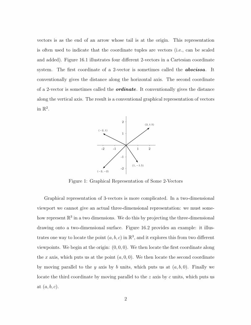
vectors is as the end of an arrow whose tail is at the origin. This representation

is often used to indicate that the coordinate tuples are vectors (i.e., can be scaled

and added). Figure 16.1 illustrates four different 2-vectors in a Cartesian coordinate

system. The first coordinate of a 2-vector is sometimes called the abscissa . It

conventionally gives the distance along the horizontal axis. The second coordinate

of a 2-vector is sometimes called the ordinate . It conventionally gives the distance

along the vertical axis. The result is a conventional graphical representation of vectors

in R2.

-2 -1 1 2

-2

-1

1

2(2, 1.5)

(1,−1.5)

(−2,−2)

(−2, 1)

Figure 1: Graphical Representation of Some 2-Vectors

Graphical representation of 3-vectors is more complicated. In a two-dimensional

viewport we cannot give an actual three-dimensional representation: we must some-

how represent R3 in a two dimensions. We do this by projecting the three-dimensional

drawing onto a two-dimensional surface. Figure 16.2 provides an example: it illus-

trates one way to locate the point (a, b, c) in R3, and it explores this from two different

viewpoints. We begin at the origin: (0, 0, 0). We then locate the first coordinate along

the x axis, which puts us at the point (a, 0, 0). We then locate the second coordinate

by moving parallel to the y axis by b units, which puts us at (a, b, 0). Finally we

locate the third coordinate by moving parallel to the z axis by c units, which puts us

at (a, b, c).

2

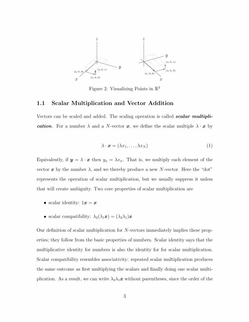
x

y

z

(a, 0, 0)

(a, b, 0)

(a, b, c)

x

y

z

(a, 0, 0)(a, b, 0)

(a, b, c)

Figure 2: Visualizing Points in R3

1.1 Scalar Multiplication and Vector Addition

Vectors can be scaled and added. The scaling operation is called scalar multipli-

cation . For a number λ and a N -vector x, we define the scalar multiple λ · x by

λ · x = (λx1, . . . , λxN) (1)

Equivalently, if y = λ · x then yn = λxn. That is, we multiply each element of the

vector x by the number λ, and we thereby produce a new N -vector. Here the “dot”

represents the operation of scalar multiplication, but we usually suppress it unless

that will create ambiguity. Two core properties of scalar multiplication are

� scalar identity: 1x = x

� scalar compatibility: λ2(λ1x) = (λ2λ1)x

Our definition of scalar multiplication for N -vectors immediately implies these prop-

erties; they follow from the basic properties of numbers. Scalar identity says that the

multiplicative identity for numbers is also the identity for for scalar multiplication.

Scalar compatibility resembles associativity: repeated scalar multiplication produces

the same outcome as first multiplying the scalars and finally doing one scalar multi-

plication. As a result, we can write λ2λ1x without parentheses, since the order of the

3

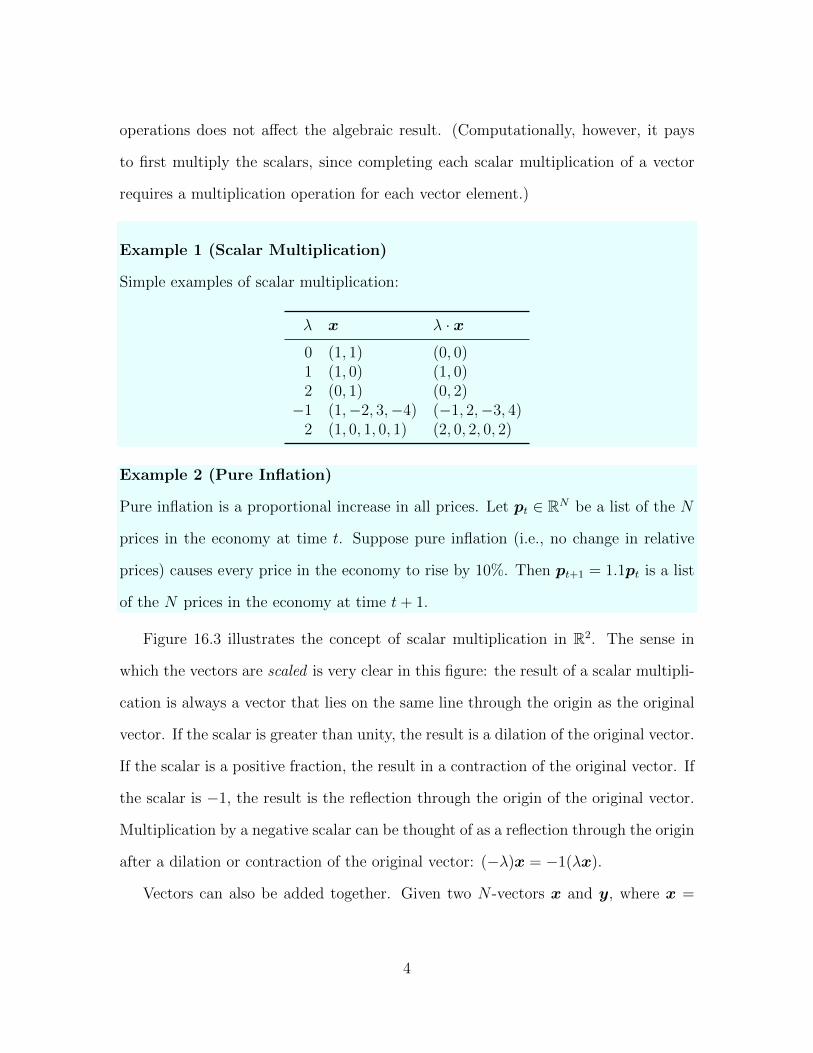
operations does not affect the algebraic result. (Computationally, however, it pays

to first multiply the scalars, since completing each scalar multiplication of a vector

requires a multiplication operation for each vector element.)

Example 1 (Scalar Multiplication)

Simple examples of scalar multiplication:

λ x λ · x0 (1, 1) (0, 0)1 (1, 0) (1, 0)2 (0, 1) (0, 2)−1 (1,−2, 3,−4) (−1, 2,−3, 4)

2 (1, 0, 1, 0, 1) (2, 0, 2, 0, 2)

Example 2 (Pure Inflation)

Pure inflation is a proportional increase in all prices. Let pt ∈ RN be a list of the N

prices in the economy at time t. Suppose pure inflation (i.e., no change in relative

prices) causes every price in the economy to rise by 10%. Then pt+1 = 1.1pt is a list

of the N prices in the economy at time t+ 1.

Figure 16.3 illustrates the concept of scalar multiplication in R2. The sense in

which the vectors are scaled is very clear in this figure: the result of a scalar multipli-

cation is always a vector that lies on the same line through the origin as the original

vector. If the scalar is greater than unity, the result is a dilation of the original vector.

If the scalar is a positive fraction, the result in a contraction of the original vector. If

the scalar is −1, the result is the reflection through the origin of the original vector.

Multiplication by a negative scalar can be thought of as a reflection through the origin

after a dilation or contraction of the original vector: (−λ)x = −1(λx).

Vectors can also be added together. Given two N -vectors x and y, where x =

4

2u

−2u

u

−0.5v

v

Figure 3: Scalar Multiplication

(x1, . . . , xN) and y = (y1, . . . , yN), we define vector addition by

x + y = (x1 + y1, . . . , xN + yN) (2)

Equivalently, if z = x + y then zn = xn + yn for every index n ∈ {1, . . . , N}. Vector

addition is an element-wise operation. That is, we add two N -vectors by summing

the corresponding elements to produce a new N -vector. To apply this definition, we

need our two vectors to have a common shape.

Example 3

Element-by-element addition of N -vectors:

(1, 2) + (3, 4) = (4, 6)

(3, 4) + (1, 2) = (4, 6)

(1, 2, 3) + (0, 0, 0) = (1, 2, 3)

(1, 2, 3) + (−1,−2,−3) = (0, 0, 0)

5

Example 4 (Aggregate Demand)

Let xk be the N -vector of excess demands (demand minus supply) that individual

k has for the N consumption goods in the economy. There are K individuals in

the economy. Aggregate excess demand is sum of individual excess demands: x =∑K

k=1 xk. We produce the aggregate excess demand vector with vector addition.

6

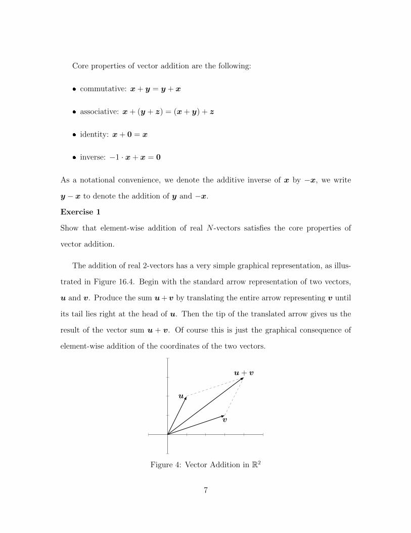
Core properties of vector addition are the following:

� commutative: x + y = y + x

� associative: x + (y + z) = (x + y) + z

� identity: x + 0 = x

� inverse: −1 · x + x = 0

As a notational convenience, we denote the additive inverse of x by −x, we write

y − x to denote the addition of y and −x.

Exercise 1

Show that element-wise addition of real N -vectors satisfies the core properties of

vector addition.

The addition of real 2-vectors has a very simple graphical representation, as illus-

trated in Figure 16.4. Begin with the standard arrow representation of two vectors,

u and v. Produce the sum u+v by translating the entire arrow representing v until

its tail lies right at the head of u. Then the tip of the translated arrow gives us the

result of the vector sum u + v. Of course this is just the graphical consequence of

element-wise addition of the coordinates of the two vectors.

u

v

u + v

Figure 4: Vector Addition in R2

7

Naturally we can equivalently translate our representation of u by v. We end up

at the same point. In Figure 16.4, the translated arrows are represented by dashed

lines. These lines are parallel to the original arrows. In this sense, the result of

vector addition can be illustrated by “completing” a parallelogram, where two sides

are provided by the original vectors.

There are two core distributive laws for scalar multiplication. First, scalar

multiplication is distributive over the addition of scalars: (λ1 + λ2)x = λ1x + λ2x.

Second, scalar multiplication is distributive over the addition of vectors: λ1(x +

y) = λ1x + λ1y. Once again, for real N -vectors, these core vector properties follow

immediately from our defintions of scalar multiplication and vector addition.

Exercise 2

Consider two real N -vectors, x and y, and two scalars, λ1 and λ2. Use the properties

of real numbers to show that the distributive laws for scalar multiplication hold.

In summary, we have defined vector addition and scalar multiplication for N -

vectors. We emphasized the following core properties of these operations:

� 1x = x and λ2(λ1x) = (λ2λ1)x.

� vector addition is associative and commutative

� the zero vector is the identity for vector addition, and every vector has an

additive inverse

� scalar multiplication is distributive over the addition of scalars and is distribu-

tive over the addition of vectors

8

1.1.1 Linear Combination

We can combine the operations of vector addition and scalar multiplication to produce

weighted sums of vectors. For example, if x and y are N -vectors, then λ1x + λ2y

is a new N -vector. It is a weighted sum of x and y, with weights λ1 and λ2. First

we scale each vector according to the rules of scalar multiplication; then we add the

results according to the rules of vector addition.

Definition 1.1 A linear combination of vectors is any finite weighted sum of

vectors. When all the weights are all nonnegative, the linear combination is also

a conical combination . When all the weights sum to 1, the linear combination

is also an affine combination . A conical, affine combination is called a convex

combination .

Definition 1.2 A vector space is a set of vectors such that any linear combination

of vectors in the set is also in the set.

Exercise 3

Consider the set of vectors in R2 constituted by all scalar multiples of the vector

(1, 1). Explain why this set is a vector space.

Once we specify how to scale and add points in the Cartesian plane, the set of all

these points constitutes a vector space. Figure 16.5 illustrates a linear combination

of two vectors in R2.

Figure 16.5 suggests that by picking the right scalars, we can produce any point

in R2 as a linear combination of the two vectors. We say that the two vectors span

R2. As long they do not lie on the same line through the origin, any two vectors span

R2. The requirement that they not lie on the same line is the requirement that they

not be scalar multiples of each other. We say they must be linearly independent.

9

−2u

−0.5v

−2u− 0.5v

uv

Figure 5: Linear Combination of Two Vectors

Definition 1.3 The linear span of a collection of vectors is the set of all possible

linear combinations of vectors in the collection. A collection of vectors is linearly

independent if no vector lies in the linear span of the rest of the collection. Equiv-

alently, there is no non-trivial linear combination of the vectors equal to 0. (A linear

combination is non-trivial if at least one of the weights is not zero.) Otherwise the

collection is linearly dependent .

Theorem 1

Suppose v′ is in the span of V , which is a finite, linearly independent collection of

N -vectors. Then the linear combination producing v′ is unique.

Proof:

Let v′ =∑N

n=1 λnvn and v′ =∑N

n=1 λ′nvn. Then 0 =

∑Nn=1(λ

′n − λn)vn.

But the vn are linearly independent, so this is only possible if for all n we

have λ′n = λn.

10

1.2 Dot Products and Linear Functions

Element-wise addition is very natural for N -vectors. We can similarly define element-

wise multiplication, which is sometimes called the Hadamard product . For exam-

ple, if a = (a1, . . . , aN) and x = (x1, . . . , xN), then their Hadamard product is

a ◦ x = (a1x1, . . . , aNxN) (3)

However it proves more useful to focus on a different concept: the dot product .

The dot product on RN is a real-valued function of two N -vectors. To produce the

dot product of two real N -vectors, we multiply the corresponding elements and then

sum the results. (Equivalently, we produce the Hadamard product and then sum its

elements.) The result is a single number, so the dot product is sometimes called the

scalar product .

a · x =N∑

n=1

anxn (4)

Exercise 4

Show that the dot product on RN has the following properties:

� positive definite (x · x ≥ 0, with equality iff x = 0)

� symmetric (x · y = y · x)

� linear in the first argument, so that (λx + y) · z = λ(x · z) + y · z

Listing 16.1 provides a pseudocode illustration of the computation of an ordinary

dot product. We define a function named dotproduct that accepts two vectors as

input arguments. We initialize that value of result to zero, and then we sequentially

add terms to this results. Each new term is produced as the product of a pair of

11

Listing 1: Vector Dot Product

#g o a l : compute o r d i n a r y d o t p r o d u c t

Function dotproduct (a : Sequence , #se q u e n c e ( an N−v e c t o r )

x : Sequence , #se q u e n c e ( an N−v e c t o r )

) → Number : #t h e d o t p r o d u c t

r e s u l t ← 0for ai , x i ∈ pairup ( a , x ) :

r e s u l t ← r e s u l t + ( a i · x i )return r e s u l t

corresponding elements of a and x.2 Once we have worked through all the pairs of

corresponding elements, we are done, and our function should return the final result.

Example 5 (Dot Product of Real Vectors)

Compute the dot product of (1, 2) and (3, 4) as follows:

(1, 2) · (3, 4) = 1 · 3 + 2 · 4 = 3 + 8 = 11

Compute the dot product of (1, 2, 3) and (4, 5, 6) as follows:

(1, 2, 3) · (4, 5, 6) = 1 · 4 + 2 · 5 + 3 · 6 = 4 + 10 + 18 = 32

Example 6 (Mean as Dot Product)

Consider an N -vector x = (x1, . . . , xN). Construct an N -vector a = (1/N, . . . , 1/N).

Then

a · x =N∑

n=1

1

Nxn =

1

N

N∑

n=1

xn

This is the arithmetic mean of the elements of x.

We will develop a variety of applications for the dot product. For the moment,

however, consider the function f(x) = a1x1 + · · · + aNxN where the an are the

2In real code, you would have to implement the pairup function. (Many languages, includingPython and Haskell, already provide a zip function to do this). Scientific programming languagesusually provide dot-product functionality. (For example, NumPy provides dot, and Mathematicaprovides Dot.)

12

parameters of the function and the xn are the variables representing the function’s N

arguments. We can write this as

f(x) = a · x (5)

Exercise 5

Let f(x) = a ·x be a real-valued function of real N -vectors. Using only the properties

established in exercise 16.4, prove that for any two N -vectors x and x′ and any scalar

λ,

f(λx + x′) = λf(x) + f(x′) (6)

Functions with this property are called linear transformations . (As an aside,

your proof for this exercise also implies that the dot product is linear in its second

argument.)

Example 7

Suppose inputs of labor (N) and capital (K) generate total production of aNN+aKK.

This is called a linear production technology , and we can represent it as the dot

product (aN , aK)·(N,K). This technology has constant returns to scale. For example,

if we double both inputs we double the output:

(aN , aK) · (2N, 2K) = 2 · (aN , aK) · (N,K)

If we increase the labor input by dN and the capital input by dK we get

(aN , aK) · (N + dN,K + dK) = (aN , aK) · (N,K) + (aN , aK) · (dN, dK)

13

1.3 Length and Distance

The conventional pictorial representation of the real number line shows any positive

real number x as lying x units to the right of 0, while any negative number x lies

x units to the left of 0. (See section ??.) The magnitude of x is thereby connected

to its distance from 0. We commonly define the distance between two points on the

number line to be the absolute value of the difference of their coordinates, and this

is a natural physical interpretation of the distance between them. For example, the

physical space between adjacent integers on a number line is constant (at one “unit”).

For any three points, x, y, and z, we note that our simple measure of distance

has the following properties:

� coincidence: d(x,y) = 0 iff x = y

� symmetry: d(x,y) = d(y,x)

� triangle inequality: d(x, z) ≤ d(x,y) + d(y, z)

The coincidence property says that there is zero distance from a point to itself; to

any other point there is a nonzero distance. The other two properties ensure that

this nonzero distance is positive. The symmetry property says that direction does

not matter for distance measurement. The triangle inequality , says it can never

be shorter to go from one point to another via a third point rather than directly. Any

function satisfying these three properties is called a distance function or metric.

Exercise 6

Show that d(x,y) > 0 whenever x 6= y, for any metric d.

Once we know how to add points and multiply them by real numbers, we may

propose two natural additions to the properties of a distance measure: translation

invariance and absolute homogeneity .

14

Figure 6: Visual Proof of Pythagorean Theorem

� d(x + z,y + z) = d(x,y).

� d(λx, λy) = |λ|d(x,y) ∀λ > 0

Translation invariance requires that distance be invariant to a common displacement.

Given our understanding of vector addition for real N -vectors, translation invariance

follows naturally. Absolute homogeneity says that “scaling” two points by the same

magnitude also scales the distance between them by that magnitude, even if we reverse

the direction. Given our understanding of scalar multiplication for real N -vectors,

absolute homogeneity follows naturally.

Exercise 7

Suppose a metric d satisfies translation invariance. Show that d(x,y) = d(−x,−y).

Suppose our vector coordinates are measured in common units. Graphically, we

use the same units of measurement to determine the location of points along each

axis. Then we can not only compute distance along each axis in a natural way;

we can compute the distance between any two points. We do this by invoking the

Pythagorean theorem, which tells us that the squared length of the hypotenuse of a

right triangle equals the sum of the squared lengths of the other two sides.3 Figure

16.6 serves as a visual proof of this theorem (?).

3The name of the theorem derives from a traditional association with Pythagoras, a Greek math-ematician of the 6th century BCE who may have given the first proof of the theorem.

15

|x1 − x0|

|y 1−y 0|

(x0, y0) (x1, y0)

(x1, y1)

√ (x1− x0

)2 + (y1− y0

)2

Figure 7: Distance between Points in R2

Consider two points in the Cartesian plane, p0 = (x0, y0) and p1 = (x1, y1),

as shown in figure 16.7. We can construct a right triangle whose horizontal side has

length |x1−x0| and whose vertical size has length |y1−y0|. The Pythagorean theorem

therefore tells us that the Euclidean length of the hypotenuse, which is the length of

line segment between the two points, is

d2(p1,p0) =√

(x1 − x0)2 + (y1 − y0)2

=√

(p1 − p0) · (p1 − p0)

(7)

Note that this measure of distance in the Cartesian plane shares core properties

with our distance measure along a line segment: symmetry, the triangle inequality,

nonnegativity, and positivity for distinct points. It also satisfies translation invariance

and absolute homogeneity.

1.4 Norms

Underpinning our notions of distance is the concept of a norm . We usually use the

notation ‖x‖ to denote the norm of a vector x. A norm is a real-valued function that is

16

absolutely homogeneous, subadditive, and separating. Any absolutely homogeneous,

subadditive function is nonnegative definite, so the final property ensures that a norm

is positive definite.

� Separating: ‖x‖ = 0 =⇒ x = 0

� Absolutely Homogeneous: ‖λx‖ = |λ| ‖x‖

� Subadditive: ‖x + y‖ ≤ ‖x‖+ ‖y‖

Exercise 8

Show the following for any real-valued function `. If ` is absolutely homogeneous, then

`(0) = 0 and `(−x) = `(x). If ` is absolutely homogeneous and subadditive, then

`(x) ≥ 0. If ` is absolutely homogeneous and separating, then `(x) = 0 ⇐⇒ x = 0.

A norm embodies some of our core intutions about length: only the zero vector

has zero length, every other vector has positive length, scaling a vector scales its

length without changing the sign, and the length of a vector sum is never greater

than the sum of the vector lengths.

Example 8 (`p-Norm)

How should we measure the length of x ∈ RN? We are most familiar with Euclidean

length: (∑N

n=1 x2n)1/2. However, many other norms are possible. For any p ≥ 1 we

can define the `p-norm as (∑N

n=1 |xn|p)1/p. Euclidean length is then the `2-norm. This

is often written as ‖x‖2, and it is often called the Euclidean norm. The `1-norm is∑N

n=1 |xn|. This is usually written as ‖x‖1, and it is often called the taxicab norm.

We also define the `∞-norm as maxn{|xn|}. This is usually written as ‖x‖∞, and it

is often called the maximum norm.

Our intuitive concepts of length and distance are tightly linked. We often think of

the length of a vector as the distance of a point from the origin. In fact, every norm

implies a corresponding metric:

17

Exercise 9

Given a norm, define the function

d(x,y) = ‖x− y‖

Show that the function d is a metric. Show that this metric also displays translation

invariance and positive homogeneity.

Example 9 (Euclidean Length and Distance)

Let x = (1, 0), so ‖x‖2 = ‖(1, 0)‖2 =√

(1, 0) · (1, 0) = 1.

Let y = (0, 1), so ‖y‖2 = ‖(0, 1)‖2 =√

(0, 1) · (0, 1) = 1.

The distance from x to y is ‖y − x‖2 = ‖(−1, 1)‖ =√

(−1, 1) · (−1, 1) =√

2.

Exercise 10

A unit vector is a vector with unit length. For any non-zero real N -vector x, prove

that (1/‖x‖2)x is a unit vector. (We call this unit vector the direction vector or

normalized vector for x.)

Exercise 11 (Cauchy-Schwarz Inequality)

Given two real N -vectors, x and y, prove that |x · y| ≤ ‖x‖ ‖y‖. (This is known as

the Cauchy-Schwarz inequality.)

Hint: Start by proving that |x · y| ≤ 1 if x and y are unit vectors.

1.5 Angle

Definition 1.4 (Angle) For any two non-zero real N -vectors x,y, we define the

angle θ between the vectors to be

θ = arccos

(x · y‖x‖‖y‖

)(8)

18

The arccosine function is the inverse of the cosine function. Since the cosine

function is periodic, we must restrict the domain of the cosine function if we want to

produce an inverse function. We define arccos only for the cosine function over the

domain [0, π]. Recall that cos(0) = 1, cos(π/2) = 0, and cos(π) = −1 (where the

angles are measured in radians).

Exercise 12 (Law of Cosines)

Suppose two sides of a triangle have lengths a and b, and the angle between them

is θ. The law of cosines for triangles says that the length c of the third side is√a2 + b2 − 2ab cos(θ). Use definition 16.4 to prove the law of cosines in R2.

Definition 1.5 (Orthogonality and Linear Dependence) Two non-zero realN -

vectors are orthogonal iff their dot product is zero: x · y = 0.

We can measure the angle between orthogonal vectors as π/2 radians (i.e., 90◦),

since cos(π/2) = 0.

And we can measure the angle between x and y as either 0 radians (i.e., 0◦) or

π radians (i.e., 180◦), depending on whether they point in the same direction or in

opposite directions. (Recall that cos(0) = 1 and cos(π) = −1.) To see the latter,

suppose y = λx, so that the two vectors are linearly dependent. Then ‖y‖ = |λ|‖x‖,

so y = ±x. So the angle between the two vectors is arccos (x · y) = arccos (±1).

19

x

y

z

y − z

Figure 8: Orthogonal Projection of y on x

Example 10

Given any two nonzero real N -vectors, x and y, we can define the orthogonal pro-

jection of y onto x by

z =y · xx · xx

The vector z is just a scaling of x such that y − z is orthogonal to x.

x · (y − z) = x · (y − y · xx · xx)

= x · y − y · xx · xx · x

= 0

This is illustrated in Figure 16.8.

1.5.1 Angles in R2

In order to gain a better understanding of the relationship between the angle between

two vectors and the dot product, we turn to R2. The top graph in figure 16.9 illustrates

the cosine of an acute angle between two unit vectors. We let our first unit vector

be (1, 0) in order to see the relationship with particular ease: the cosine of an acute

angle is clearly positive but less than one. The bottom graph in figure 16.9 illustrates

the cosine of an obtuse angle between two unit vectors. Again we let our first unit

vector be (1, 0) in order to see the relationship with particular ease: the cosine of an

20

(x, y)sin(θ)

cos(θ)

θ

-1 0 1

(x, y)sin(θ)

cos(θ)

θ

-1 0 1

Figure 9: Angle and Cosine

obtuse angle is clearly negative but greater than negative one. We see that the cosine

varies from 1 to 0 to −1 as the angle varies from 0 to π/2 to π radians. In each case

the cosine of the angle is just the first coordinate of the second vector. Note that the

dot product (1, 0) · (x, y) = x returns this first coordinate, which is the cosine of the

angle.

We can apply this insight to any two vectors. The key observation is that if we

rotate two vectors by the same amount, this will not change the angle between them.

For a given the angle of rotation θ, let c = cos(θ) and s = sin(θ). If we rotate two

points, (x, y) and (x′, y′) through the counterclockwise angle θ, we end up with two

new points, (cx− sy, sx + cy) and (cx′ − sy′, sx′ + cy′).4 Recalling that s2 + c2 = 1,

the dot product of these two new vectors is just xx′ + yy′, identical to the vectors

before rotation. This is just another way of saying that the angle between them is

unchanged.

4See chapter ?? for discussion.

21

In figure 16.10, we illustrate the case where our vectors are both are in the second

quadrant. First we scale them to produce unit vectors. Here u and v are the nor-

malized vectors (they have the same direction but unit length). (See exercise 16.10.)

Then rotate them so that one becomes the standard unit vector along the x-axis and

the other is in the first two quadrants, matching one of the two examples in figure

16.9. Neither of these operations (scaling and rotating) changes the angle between

the vectors, so afterwards we can determine that angle as in Figure 16.9.

θ

-1 0 1

u

v

θ

-1 0 1

u

v

Figure 10: Angle Preserving Scaling and Rotation

2 Equations and Implicit Functions

Given a function f(x) the graph of the equation f(x) = 0 is the set of values of x

such that the equation is satisfied. These values are called the zeros of the function.

They are also called the solution set of the equation f(x) = 0. The zero vector

is always a zero of a linear transformation. For example, suppose f is has the form

22

x1

x2

a· x

=0

a

Figure 11: Null Space of a Vector

(16.5): we can readily see that a · 0 = 0.

2.1 Linear Equations

A linear transformation may have multiple zeros. The set of zeros is called the null

space (or kernel) of the linear transformation. For example, the null space of the

real N -vector a is null(a) = {x | a · x = 0}. Vectors in null(a) are said to be

orthogonal to a. Figure 16.11 illustrates this graphically in the Cartesian plane.

We see that points in null(a) constitute a line that is perpendicular to a.

Exercise 13 (Null Space is a Vector Space)

For any vector a, prove that null(a) is a vector space.

23

Example 11 (Null Space of a 2-Vector)

Suppose f(x) = (3/2)x1− (1/2)x2. Then the null space of f is the set of pairs x1 and

x2 such that

3

2x1 −

1

2x2 = 0

Solving for x2 in terms of x1, we find that the null space comprises all the points on

the line through the origin described by

x2 = 3x1

Example 12 (Purchasing Power Parity)

International economists have researched the possibility that the spot rate (S) be-

tween two countries’ currencies is eventually related to the relative price level (P) of

the two countries by a constant of proportionality (q). Write the deviation of the

spot rate from its long-run level as

f(S,P) = S − qP

In full equilibrium, f(S,P) = 0, so that

S − qP = 0

This relationship is known as long-run purchasing power parity. It implicitly deter-

mines S as a function of P, but it is most often represented by explicitly solving for

S.

S = qP

Examples 16.11 and 16.12 suggest that if an equation involves multiple variables, it

may implicitly define one of them as a function of the rest. In the function is nonlinear,

24

however, the equation may imply a relation that has no functional representation. For

example, if f(x, y) = x2 + y2 − 1, then f(x, y) = 0 characterizes the unit circle.

Let us find a point on a line determined by x and y that minimizes the distance

to a point p0. Recall that points on the line can be written as x + λ(y − x). We use

the fact that the shortest distance will be determined by a perpendicular. That is

[p0 − x− λ(y − x)] · (y − x) = 0

(p0 − x) · (y − x) = λ(y − x) · (y − x)

λ =(p0 − x) · (y − x)

(y − x) · (y − x)

(9)

2.2 Affine Equations

We have seen that the dot product turns any N -vector a into a linear transformation,

f(x) = a · x. We defined null(a) to be the set of points such that a · x = 0. This is

one example of a level set : a set of points such that f(x) = b for some constant b.

We now consider what level sets of linear transformations look like for nonzero values

of b.

Recall that a real N -vector a has an associated linear equation a · x = 0. To

represent other level sets, we can use an affine equation. An affine equation for a

can be written as

a · x = b (10)

Changes in the constant b translate (i.e., shift) the locus of points satisfying this

equation.

Affine equations have a nice graphical representation in the Cartesian plane. Sup-

25

pose a = (a1, a2), so our affine equation in two variables can be written as

a1x1 + a2x2 = b (11)

where a1 and a2 are not both zero. The graph of such an affine equation is a straight

line, and every straight line can be represented by an affine equation. (Such equations

are therefore often called linear rather than affine, although strictly speaking we

reserve the term ‘linear’ for the case b = 0.) We may therefore call (16.11) the

general equation of a line in R2.

Example 13

Consider the affine equation

3

2x1 −

1

3x2 =

2

3

Solving for x2 in terms of x1, we get an equivalent equation that is often called the

slope-intercept form for this line.

x2 = 4.5x1 − 2

The solution set comprises all the points on the line described by either equation.

Figure 16.12 illustrates this with an example in the Cartesian plane. Note that

the level sets are all parallel. We have seen that every point in null(a) is orthogonal

to a, so every level set is in that sense perpendicular to a. To capture this sense of

perpendicularity, we say that a is normal vector to the level set.

26

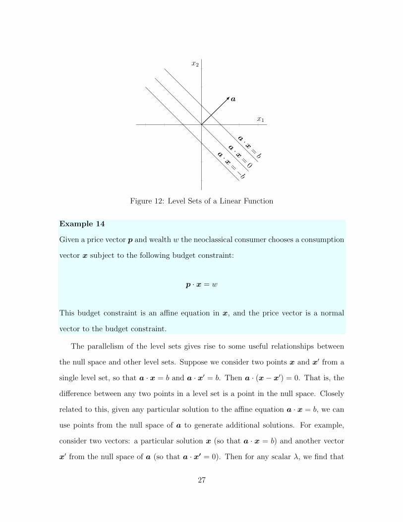
x1

x2

a · x=b

a · x=

0

a · x= −

b

a

Figure 12: Level Sets of a Linear Function

Example 14

Given a price vector p and wealth w the neoclassical consumer chooses a consumption

vector x subject to the following budget constraint:

p · x = w

This budget constraint is an affine equation in x, and the price vector is a normal

vector to the budget constraint.

The parallelism of the level sets gives rise to some useful relationships between

the null space and other level sets. Suppose we consider two points x and x′ from a

single level set, so that a · x = b and a · x′ = b. Then a · (x− x′) = 0. That is, the

difference between any two points in a level set is a point in the null space. Closely

related to this, given any particular solution to the affine equation a · x = b, we can

use points from the null space of a to generate additional solutions. For example,

consider two vectors: a particular solution x (so that a · x = b) and another vector

x′ from the null space of a (so that a · x′ = 0). Then for any scalar λ, we find that

27

x + λx′ also satisfies the affine equation. That is, a · (x + λx′) = b.

2.3 Systems of Affine Equations

Consider a vector a and another vector b ∈ null(a). Consider any conical combination

x = λ1a+λ2b, where λ1, λ2 ≥ 0. Then a·x = λ1a·a ≥ 0. We will call the set of such

conical combinations the nonnegative half-space generated by a. If we subtract the

null space, we get the positive half-space. The nonpositive and negative half-spaces

are defined symmetrically.

Many economic models involve numerous equations and unknowns. Suppose we

have a system of R affine equations in K unknowns, x1, . . . , xK .

a11x1 + a12x2 + · · ·+ a1KxK = b1

a21x1 + a22x2 + · · ·+ a2KxK = b2

...

aR1x1 + aR2x2 + · · ·+ aRKxK = bR

(12)

We call this a system of linear equations. We refer to the xk as unknowns or

endogenous variables. We refer to the br as constants , exogenous values, or

targets . We refer to the ark as coefficients . Given values for all the coefficients

and targets, if we can find values for the unknowns that simultaneously satisfy all

the equalities, we say the system is consistent . Otherwise, we say the system is

inconsistent . Equation (16.12) is a rather compact representation of an arbitrarily

large system of equations, but we are going to develop a still more compact and more

useful representation.

We know that we can use the dot product to more compactly represent each one

28

of these. Consider the r-th equation in (16.12).

ar1x1 + ar2x2 + · · ·+ arKxK = br (13)

Let us introduce the notation

Ar : = (ar1, ar2, . . . , arK) (14)

Then we can rewrite (16.13) as

Ar : · x = br (15)

In fact, we can rewrite the entire system as

A1 : · x = b1

A2 : · x = b2

...

AR : · x = bR

(16)

Our next step is to generalize our dot product so that we can represent this

entire system of equations as A · x = b. This generalization is known as matrix

multiplication. We introduce matrices and matrix multiplication in chapter ??.

Supplementary Reading

?, ch.4,5, ?, ch.4

29

Problems for ReviewExercise 14

Here are some popular forms of affine equations in two variables.

y = mx+ b slope-intercept

y − y1 = m(x− x1) point-slope

x

a+y

b= 1 double-intercept

x = at+ b and y = ct+ d parametric form, t ∈ R

Begin with the general equation of a line as given in (16.11). Convert that equa-

tion to the following forms: slope-intercept form, point-slope form (for arbitrary x1),

double-intercept form, and parametric form. Do any particular parameter values raise

problems for any of these representations?

Computational Exercises

Computational Exercise 1

Implement a function named dotproduct that implements the algorithm in Listing

??. The function should take two input arguments (the vectors), the type of which

may depend on how you choose to represent real N -vectors. The function should

return a real number. Additionally, implement error-checking code that ensures that

the two input arguments have the same length.

Computational Exercise 2

Implement a function named norm2 that computes the Euclidean norm for any real

N -vector. The function should take one input argument (the vector), the type of

which may depend on how you choose to represent real N -vectors. The function

should return a non-negative real number.

30

Computational Exercise 3

Implement a function named angle that computes the angle (in radians) between

any two real N -vectors. The function should take two input arguments (the vectors),

the type of which may depend on how you choose to represent real N -vectors. The

function should return a real number in [0, π]. Make use of your previous work in

computational exercises 16.1 and 16.2.

31

Matrices and Linear Models

114

Economists encounter and matrices in economic theory, econometric theory, and

econometric applications. Two core reasons for this ubiquity are notational compact-

ness and computational convenience. In the present chapter, we will learn enough

about matrices to undertake some economic applications.

1 Introduction to Matrices

Matrix notation is remarkably compact. For example, we will see that an arbitrarily

large system of linear equations can be represented as

A · x = b (1)

In many interesting systems there is a unique solution for the unknowns x that can

be represented with equal compactness as

x = A−1 · b (2)

Here the matrix A−1 is called the multiplicative inverse of the matrix A. In this

chapter, we will learn enough about matrices to understand these usages.

1.1 Describing Matrices

A matrix is a rectangular array of elements. If all the elements are real numbers, it

is called a real matrix. If a matrix has R rows and K columns, we say that it is an

R by K matrix, or that the order of the matrix is R ×K. Equivalently, we say it

has shape (R,K). The numbers R and K are called the dimensions of the matrix.

Note that we state the row dimension first and then the column dimension. When

1

we need to be explicit about a matrix’s shape, we sometimes add a subscript to its

name: AR×K .

Example 1 (Matrix Shape)

Consider the following three matrices.

A3×2 =

2 3

5 6

1 3

B3×1 =

3

4

5

C1×3 =

[1 2 −5

]

In this example A is a 3 by 2 matrix: its shape is (3, 2), its row dimension is 3,

and its column dimension is 2. Similarly, B is a 3 by 1 matrix, and C is a 1 by 3

matrix. In each case the shape is communicated by a subscript to the matrix name.

Of course, in such simple examples, the shape is also easily determined by inspection

of the matrix.

Since a matrix is a rectangular array, each element can be uniquely identified

by its row index and column index. For an arbitrary matrix A, let ark denote the

element in row r and column k. Note that we first list the row index and then the

column index. When we need to emphasize the indices, we often represent the matrix

A with the more explicit notation [ark]. Here is an expanded representation of an

2

R×K matrix:

AR×K =

a11 a12 . . . a1k . . . a1K

a21 a22 . . . a2k . . . a2K...

......

...

ar1 ar2 . . . ark . . . arK ← row r

......

......

aR1 aR2 . . . aRk . . . aRK

↑column k

(3)

Matrix equality is element-wise: equal matrices have the same shape, and corre-

sponding elements are equal.

A = B ⇐⇒ ark = brk ∀r, k (4)

A matrix consisting ofR rows and only one column is often called anR-dimensional

column vector. It is a R× 1 matrix. A matrix consisting of K columns and only one

row is often called a K-dimensional row vector. It is a 1×K matrix. The elements of

a row vector or column vector are often identified by a single index, since this creates

no ambiguity in identifying the element.

1.2 Matrices are Vectors

Matrices are rectangular arrays of elements that have certain properties. Crucially,

we define scalar multiplication and element-wise addition for matrices. These will

give us all the core vector properties, which means that we can consider any matrix

to be a vector. For example, a real matrix is an element of the vector space of all real

matrices with the same shape.

3

For a matrix A = [ark] and a scalar λ we define

λ ·A = [λark] (5)

That is, we multiply every element by that scalar. (As a matter of notation, it is

conventional to suppress the “dot” operator unless doing so will create confusion.)

Example 2 (Scalar Multiplication)

2 ·

1 5

6 8

=

2 · 1 2 · 5

2 · 6 2 · 8

=

2 10

12 16

Matrices are added element-by-element. This means we can only add matrices that

have the same shape. We say that matrices with the same shape are conformable

for addition. Given two matrices A and B with the same shape, we define

A + B = [ark + brk] (6)

That is, the new matrix has the same shape, and each element is the sum of the

corresponding elements of A and B.

Example 3 (Matrix Addition)

1 2 3

4 5 6

+

7 8 9

10 11 12

=

1 + 7 2 + 8 3 + 9

4 + 10 5 + 11 6 + 12

=

8 10 12

14 16 18

Addition takes place element by element. If C = A + B, then cij = aij + bij.

So the associativity of matrix addition follows from the associativity of addition of

the matrix elements. For example, the addition of real numbers is associative, so the

4

addition of real matrices is associative.

(A + B) + C = [(ark + brk) + crk] = [ark + (brk + crk)] = A + (B + C) (7)

Similarly, from the commutativity of the addition of real numbers, we know that the

addition of real matrices is commutative.

Example 4 (Matrix Addition Commutes)

Here we use the two matrices

A =

4 7

3 2

B =

1 5

6 8

to illustrate the commutativity of matrix addition.

A + B =

4 + 1 7 + 5

3 + 6 2 + 8

=

5 12

9 10

=

1 + 4 5 + 7

6 + 3 8 + 2

= B + A

A matrix with only zero elements is called a zero matrix (or null matrix ). Note

that for the set of R × K matrices, the conformable zero matrix is is the additive

identity. That is, if A and 0 both have dimensions R×K, then

A + 0 = A and 0 + A = A (8)

Note that 0R×K is the only additive identity for R by K matrices. If A is an

additive identity, then A + 0 = 0 but A + 0 = A, so A = 0. Identity is unique.

We use the notation −A denote the additive inverse of any matrix A. Given a

conformable matrix B, we write B−A as shorthand for B+(−A). Because addition

is element-by-element, we can construct the additive inverse of A using the additive

5

inverses of the elements.

[ark] + [−ark] = 0 (9)

Recalling our definition of scalar multiplication, we see that −1 · A is the additive

inverse of any matrix A. That is, −A = −1 ·A.

Example 5

Given the two matrices

A =

4 7

3 2

B =

1 5

6 8

we can form the difference A−B as

A−B =

4− 1 7− 5

3− 6 2− 8

=

3 2

−3 −6

So we can see that matrix subtraction is element-by-element.

Naturally, we have the two usual distributive properties for scalar multiplication.

These follow immediately from our definitions of scalar multiplication and matrix

addition.

(α + β)A = αA + βA

α(A + B) = αA + αB

(10)

1.3 Matrix Multiplication

Given two matrices AR×N and BN×K , we define the matrix product A · B as

follows:

C = A ·B =⇒ crk =N∑

n=1

arnbnk (11)

6

The matrix product is also called a dot product . Here A is the premultiplying

matrix, and B is the postmultiplying matrix. Although we sometimes write the

matrix product of A and B with an explicit operator (e.g., A ·B), it is common to

simply write AB.1

Our definition requires that the premultiplying matrix has the same number of

columns as the postmultiplying matrix has rows. Matrices with such compatible

shapes are said to be conformable for multiplication. The matrix product will have

as many rows as the premultiplying matrix and as many columns as the postmulti-

plying matrix. So in this case, C must have shape (R,K).

Example 6 (Matrix Multiplication)

Consider the two matrices

A =

[1 2

]B =

3

4

Form the matrix products AB and BA as follows:

AB =

[1 2

]

3

4

=

[1 · 3 + 2 · 4

]=

[11

]

BA =

3

4

[1 2

]=

3 · 1 3 · 2

4 · 1 4 · 2

=

3 6

4 8

Taking a close look at (11), we see that each element of A ·B is an ordinary dot

product of a row of the premultiplying matrix (A) and a column of the postmulti-

plying matrix (B). The r, k-th element of the matrix product is the dot product of

1Using adjacency to indicate the matrix dot product is common in mathematics texts but lesscommon computationally. E.g., in Mathematica, a space between two matrix is an implicit Timescommand, which produces the Hadamard (elementwise) product.

7

a11 . . . a1n . . . a1N

.... . .

......

...

ar1 . . . arn . . . arN

......

.... . .

...

aR1 . . . aRn . . . aRN

A : R rows, N columns

b11 . . . b1k . . . b1K

.... . .

......

...

bn1 . . . bnk . . . bnK

......

.... . .

...

bN1 . . . bNk . . . bNK

B : N rows, K columns

c11 . . . c1k . . . c1K

.... . .

......

...

cr1 . . . crk . . . crK

......

.... . .

...

cR1 . . . cRk . . . cRK

C = A ·B : R rows, K columns

a r1×b

1k

arn×b

nk

a rN×bN

k

+ . . .+

+ . . .+

Figure 1: Falk’s Scheme for Matrix Multiplication

8

the r-th row of A and the k-th column of B. Let Ar : be the vector representing the

r-th row of A, and let B : k be the vector representing the k-th column of B. Then

C = A ·B =⇒ crk = Ar : ·B : k (12)

Example 7 (Matrix Dot Product)

Consider the three matrices

A =

[2 35 6

]B =

[84

]C =

[8 14 2

]

We will compute AB and AC.First we find the matrix product AB. In this case, a 2 × 2 matrix premultiplies

a 2× 1 matrix, yielding a 2× 1 matrix.

AB =

[2 35 6

] [84

]=

[(2, 3) · (8, 4)(5, 6) · (8, 4)

]=

[2864

]

Next we find the matrix product AC. In this case, a 2 × 2 matrix premultipliesa 2× 2 matrix, yielding a 2× 2 matrix.

AC =

[2 35 6

] [8 14 2

]=

[(2, 3) · (8, 4) (2, 3) · (1, 2)(5, 6) · (8, 4) (5, 6) · (1, 2)

]=

[28 864 17

]

Note that because the first (and only) column of B has the same elements as the firstcolumn of C, the first (and only) column of AB has the same elements as the firstcolumn of AC.

Exercise 1 (Matrix Multiplication Associates)

Prove that multiplication is associative. That is, for any three conformable matrices

A, B, and C, we have

A(BC) = (AB)C

9

1.3.1 Two Equations in Two Unknowns

Consider the following 2× 2 matrix and 2× 1 column vector.

A =

a11 a12

a21 a22

x =

x1

x2

(13)

Use our definition of matrix multiplication to form the matrix product Ax.

Ax =

a11 a12

a21 a22

x1

x2

def

=

a11x1 + a12x2

a21x1 + a22x2

(14)

Consider a two-equation system in two unknowns (x1 and x2):

a11x1 + a12x2 = b1

a21x1 + a22x2 = b2

(15)

We will write this system in the form Ax = b. For our two-equation system, x and b

are each 2× 1 matrices (i.e., column vectors). Since the column index does not vary

across the elements of x and b, we follow the convention of suppressing it. So we have

A =

a11 a12

a21 a22

x =

x1

x2

b =

b1

b2

(16)

We will represent the left hand side of (15) by the matrix product Ax, invoking our

definitions of matrix equality and matrix multiplication. Similarly, b can represent

the right hand side of (15).

10

We can now write Ax = b more explicitly for our two-equation system.

a11 a12

a21 a22

x1

x2

=

b1

b2

(17)

Corresponding to the coefficient matrix A we have the rows

A1 : = [a11 a12]

A2 : = [a21 a22]

Clearly each row of the coefficient matrix contains the coefficients of one equation.

In more detail, the first equation of our two equation system can be written as

[a11 a12

]x1

x2

= [b1] (18)

Recall that a 1× 2 matrix multiplied by a 2× 1 matrix yields a 1× 1 matrix. We can

perform the matrix multiplication on the left to get

[a11x1 + a12x2] = [b1] (19)

which equates two 1× 1 matrices.

11

Example 8 (Matrix Representation: 2 Equations with 2 Unknowns)

Consider the two-equation system

x1 + 2x2 = 5 3x1 + 4x2 = 6

Here we have two equations in two unknowns, x1 and x2, and we want to write this

system in the form Ax = b. The coefficients from each equation will be the rows of

our coefficient matrix.

A1 : = [1 2] A2 : = [3 4]

So we can represent the system as

1 2

3 4

x1

x2

=

5

6

Exercise 2

A simple “Keynesian” IS-LM model can be written as

Y = a− βR

m = κY − γR

where the endogenous variables (“unknowns”) are Y and R and the exogenous vari-

ables (“constants”) are a and m. Write the model as a matrix equation in the form

Ax = b.

With this understanding of matrix multiplication, we can write the any system

of linear equations as A · x = b. To do so, we need to construct three matrices: a

matrix A of coefficients, a matrix x of unknowns (often called endogenous variables),

and a matrix b of right-hand-side constants (often called exogenous variables). First,

12

collect the coefficients (ark) of the system in a matrix. As suggested by the labeling,

all the coefficients for the r-th equation are in the r-th row of the coefficient matrix.

Then let x be the K-dimensional column vector whose k-th element is xk and b be

the R-dimensional column vector whose r-th element is br. We see that our definition

of matrix multiplication allows convenient and compact representation of systems of

linear equations.

Example 9 (Linear Transformation)

Consider any R ×K matrix of real numbers, A = [ark]. Let us define a function f

by the following mapping:

x1

x2...

xK

f7→

∑Kk=1 a1kxk

∑Kk=1 a2kxk

...∑K

k=1 aRkxk

The function f takes a K-dimensional column vector as an argument and returns an

R-dimensional column vector. (That is, f : <K → <R.) We can write this compactly

as f(x)def= Ax. As discussed in chapter ??, the function f is a linear transformation.

1.3.2 Matrix Multiplication Does Not Commute

The associative property holds for matrix multiplication. If we look at a typical

element, associativity follows from our ability to change the order of summation.

(AB)C =

[∑

j

(∑

i

aribij)cjk

]=

[∑

i

ari(∑

j

bijcjk)]

= A(BC) (20)

We can equivalently note that (AB)C = A(BC) because for all r, k we have

(Ar :B)C : k = Ar :(BC : k). Since the associativity of matrix multiplication tells us

13

that the order in which we elect to perform our matrix multiplications is irrelevant,

we often simply omit parentheses for matrix products. For example, we write (AB)C

and A(BC) simply as ABC.

Exercise 3

Given the three matrices

A =

1 2

3 4

B =

5 6

7 8

C =

9 10

11 12

Calculate the element in the second row and first column of ABC. Do not calculate

any other elements of this product. Be sure to explain what you are doing.

The commutative property does not hold for matrix multiplication. For one

thing, there is an issue of conformity: BA may not be defined even if AB is. Even

when both products are defined, they may yield matrices of different dimensions. And

even when both matrices are square, AB will generally differ from BA.

Example 10

Suppose we have two 2× 2 matrices A and B defined as

A =

4 7

3 2

, B =

1 5

6 8

Then AB and BA can be calculated as

AB =

46 76

15 31

, BA =

19 17

48 58

Thus AB does not does not generally equal BA.

14

Since matrix multiplication is not commutative, there are two separate distribu-

tive laws for matrices: one for premultiplication and one for postmultiplication.

A(B + C) = AB + AC

(B + C)A = BA + CA

(21)

We will give a brief proof of the distributive law for premultiplication.

Proof:

Consider the r, k-th element.

Ar :(B : k + C : k) =I∑

i=1

[ari(bik + cik)]

=I∑

i=1

(aribik + aricik)

=I∑

i=1

aribik +I∑

i=1

aricik

= Ar :B : k + Ar :C : k

(22)

Exercise 4

Prove the distributive law for postmultiplication: (B + C)A = BA + CA.

Exercise 5

Prove the two distributive properties of scalar multiplication.

2 Matrix Identity and Matrix Inverse

Definition 2.1 A square matrix has the same number of rows and columns; this

number is called the order of the matrix. A diagonal matrix is a square matrix

15

with zero elements everywhere except on its principal diagonal. A scalar matrix is

a diagonal matrix with the same value for every element on the principal diagonal.

2.1 Multiplicative Identity

To go along with our definition of matrix multiplication, we can find a multiplicative

identity.

Definition 2.2 An identity matrix of order N is a scalar matrix of order N whose

value on the principal diagonal is unity. That is, its elements are 0 except along the

principal diagonal, where each element is 1. We sometimes represent this as I = [δrk],

where δrk is the so-called Kronecker delta :

δrk =

1, if r = k

0, otherwise

Often we are not explicit about the order of an identity matrix: we simply write I,

allowing the order to be inferred from context.

Each column of IN contains an N -dimensional standard unit vector . Recall

that the k-th N -dimensional standard unit vector has all elements 0 except for the

k-th, which is 1. Clearly there are N distinct unit N -vectors. For an identity matrix

I, the k-th column (I : k) is the k-th standard unit vector.

16

Example 11 (Identity Matrices)

Here are three identity matrices:

I1 = [1] I2 =

1 0

0 1

I3 =

1 0 0

0 1 0

0 0 1

From our definition of matrix multiplication, if the matrix A has shape R ×K,

then

IRA = A = AIK (23)

In this sense, multiplication by the identity matrix has no effect. For example, if we

restrict our attention to the set of 2× 2 matrices, then for any matrix A

I2A2×2 = A2×2 = A2×2I2 (24)

That is, I2 is the multiplicative identity for the set of 2× 2 matrices. Similarly, I3 is

the multiplicative identity for the set of 3× 3 matrices, and so on.

The multiplicative identity of any order is unique. Suppose IN and JN are both

multiplicative identities. Then INJN = JN and INJN = IN so IN = JN .

17

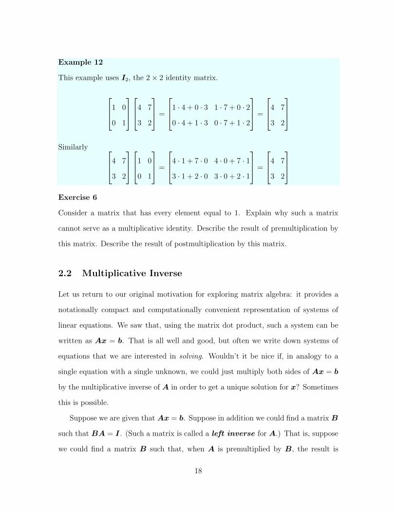
Example 12

This example uses I2, the 2× 2 identity matrix.

1 0

0 1

4 7

3 2

=

1 · 4 + 0 · 3 1 · 7 + 0 · 2

0 · 4 + 1 · 3 0 · 7 + 1 · 2

=

4 7

3 2

Similarly

4 7

3 2

1 0

0 1

=

4 · 1 + 7 · 0 4 · 0 + 7 · 1

3 · 1 + 2 · 0 3 · 0 + 2 · 1

=

4 7

3 2

Exercise 6

Consider a matrix that has every element equal to 1. Explain why such a matrix

cannot serve as a multiplicative identity. Describe the result of premultiplication by

this matrix. Describe the result of postmultiplication by this matrix.

2.2 Multiplicative Inverse

Let us return to our original motivation for exploring matrix algebra: it provides a

notationally compact and computationally convenient representation of systems of

linear equations. We saw that, using the matrix dot product, such a system can be

written as Ax = b. That is all well and good, but often we write down systems of

equations that we are interested in solving. Wouldn’t it be nice if, in analogy to a

single equation with a single unknown, we could just multiply both sides of Ax = b

by the multiplicative inverse of A in order to get a unique solution for x? Sometimes

this is possible.

Suppose we are given that Ax = b. Suppose in addition we could find a matrix B

such that BA = I. (Such a matrix is called a left inverse for A.) That is, suppose

we could find a matrix B such that, when A is premultiplied by B, the result is

18

an identity matrix. If we can find such a matrix, then we can isolate the vector of

unknowns as follows.

Ax = b

B(Ax) = Bb

(BA)x = Bb

Ix = Bb

x = Bb

(25)

The third step uses the associativity of matrix multiplication, which we showed in

exercise 1. (Also see section 1.3.2.)

Next, we would like x = Bb to be a solution to our system of equations in the

following natural sense: we want to be able to substitute our solution for x and satisfy

the equation as an identity. This is possible if B is a right inverse for A, which

means that AB = I. Then we have

Ax = A(Bb) = (AB)b = Ib = b (26)

Definition 2.3 (Matrix Inverse) If BA = I we call B a left inverse for A, and

we call A a right inverse for B. If a matrix A has both a left inverse and a right

inverse, we say that A is invertible or nonsingular . If A is not invertible, we say

it is singular or degenerate .

Theorem 1 (Unique Inverse)

If matrix AR×K has a left inverse B and a right inverse C, then B = C.

Proof:

We are given that BA = IK and AC = IR. Note that, since identity

19

matrices are square, B and C must both be K×R matrices. Since matrix

multiplication is associative, we have B = B(AC) = (BA)C = C.

We use the notation A−1 to denote the inverse of a the nonsingular matrix A.

We read A−1 as “A inverse”. Eventually we will show that only square matrices are

invertible (and not all of those). Consider any invertible matrix AN×N , with inverse

A−1. Then

A−1A = AA−1 = IN (27)

How can we find the inverse of a matrix A, assuming it exists? For the case of

2× 2 matrices, we can follow a simple rule.

A =

a b

c d

=⇒ A−1 =

1

ad− bc

d −b

−c a

(28)

Exercise 7

Suppose A2×2 has a nonzero determinant. Use our rule for 2×2 matrices to construct

an inverse A−1. Show that A−1A = I2 and that AA−1 = I2.

Equation (28) makes use of scalar multiplication. Recall from section 1.1 that

λA = [λark]: we multiply each element of the matrix by the same scalar, which in

this case is the number 1/(ad−bc). The number ad−bc is known as the determinant

of our 2 × 2 matrix, and it determines whether we can find an inverse. We denote

this determinate by |A|. If ad = bc then |A| = 0 and our matrix does not have a

multiplicative inverse. (We will return to this.) The 2 × 2 matrix on the right of

(28) is called the adjugate of A, which we denote by A#. With this notation, when

|A| 6= 0, we can write

A−1 =1

|A|A# (29)

20

Example 13

This example uses our rule for 2× 2 matrices to produce an inverse matrix.

A =

2 4

6 8

=⇒ |A| = −8 A# =

8 −4

−6 2

This gives us the matrix inverse:

A−1 =1

−8

8 −4

−6 2

=

−1.0 0.50

0.75 −0.25

We can easily check that A−1A = I2 and that AA−1 = I2. For example,

A−1A =

−2 + 3 −4 + 4

1.5− 1.5 3− 2

=

1 0

0 1

Exercise 8

For any nonsingular N × N matrices A and B, prove that (A−1)−1 = A and that

(AB)−1 = B−1A−1.

21

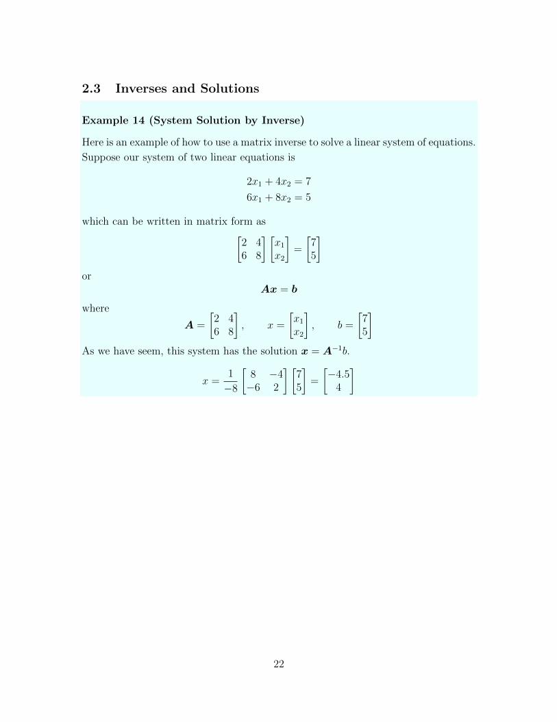
2.3 Inverses and Solutions

Example 14 (System Solution by Inverse)

Here is an example of how to use a matrix inverse to solve a linear system of equations.

Suppose our system of two linear equations is

2x1 + 4x2 = 7

6x1 + 8x2 = 5

which can be written in matrix form as[2 46 8

] [x1x2

]=

[75

]

orAx = b

where

A =

[2 46 8

], x =

[x1x2

], b =

[75

]

As we have seem, this system has the solution x = A−1b.

x =1

−8

[8 −4−6 2

] [75

]=

[−4.5

4

]

22

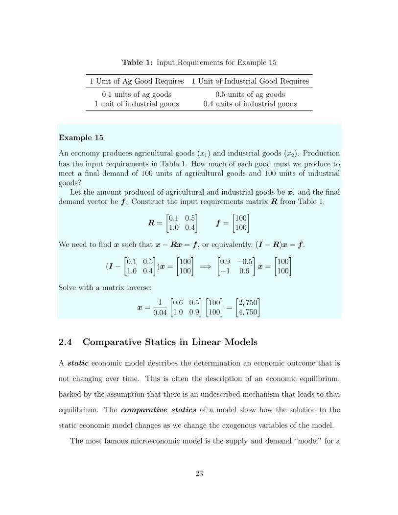
Table 1: Input Requirements for Example 15

1 Unit of Ag Good Requires 1 Unit of Industrial Good Requires

0.1 units of ag goods 0.5 units of ag goods1 unit of industrial goods 0.4 units of industrial goods

Example 15

An economy produces agricultural goods (x1) and industrial goods (x2). Production

has the input requirements in Table 1. How much of each good must we produce tomeet a final demand of 100 units of agricultural goods and 100 units of industrialgoods?

Let the amount produced of agricultural and industrial goods be x. and the finaldemand vector be f . Construct the input requirements matrix R from Table 1.

R =

[0.1 0.51.0 0.4

]f =

[100100

]

We need to find x such that x−Rx = f , or equivalently, (I −R)x = f .

(I −[0.1 0.51.0 0.4

])x =

[100100

]=⇒

[0.9 −0.5−1 0.6

]x =

[100100

]

Solve with a matrix inverse:

x =1

0.04

[0.6 0.51.0 0.9

] [100100

]=

[2, 7504, 750

]

2.4 Comparative Statics in Linear Models

A static economic model describes the determination an economic outcome that is

not changing over time. This is often the description of an economic equilibrium,

backed by the assumption that there is an undescribed mechanism that leads to that

equilibrium. The comparative statics of a model show how the solution to the

static economic model changes as we change the exogenous variables of the model.

The most famous microeconomic model is the supply and demand “model” for a

23

single market. Let us lay this out as a simple linear model of an agricultural good.

Q = s0 + s1P − s2W (Supply)

Q = d0 − d1P + d2I (Demand)

The model parameters are the si and the di coefficients. The model variables are Q,

P , W , and I: the quantity supplied and demand (in equilibrium), the market price,

a bad weather measure, and consumer income. We will solve for the endogenous

variable Q and P in terms of the exogenous variables W and I.

First rewrite the system of linear equations by moving the terms in the endogenous

variables to the left and everything else to the right.

Q− s1P = s0 − s2W (Supply)

Q+ d1P = d0 + d2I (Demand)

Next express this system of linear equations in matrix notation:

1 −s11 d1

Q

P

=

s0 − s2W

d0 + d2I

(30)

Our system now has the form Ax = b. We have seen that we can solve such a

system for x = A−1b.

Q

P

=

1 −s11 d1

−1 s0 − s2W

d0 + d2I

=1

d1 + s1

d1 s1

−1 1

s0 − s2W

d0 + d2I

(31)

24

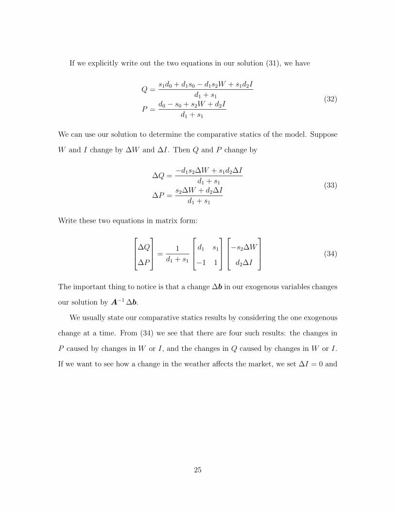
If we explicitly write out the two equations in our solution (31), we have

Q =s1d0 + d1s0 − d1s2W + s1d2I

d1 + s1

P =d0 − s0 + s2W + d2I

d1 + s1

(32)

We can use our solution to determine the comparative statics of the model. Suppose

W and I change by ∆W and ∆I. Then Q and P change by

∆Q =−d1s2∆W + s1d2∆I

d1 + s1

∆P =s2∆W + d2∆I

d1 + s1

(33)

Write these two equations in matrix form:

∆Q

∆P

=

1

d1 + s1

d1 s1

−1 1

−s2∆W

d2∆I

(34)

The important thing to notice is that a change ∆b in our exogenous variables changes

our solution by A−1 ∆b.

We usually state our comparative statics results by considering the one exogenous

change at a time. From (34) we see that there are four such results: the changes in

P caused by changes in W or I, and the changes in Q caused by changes in W or I.

If we want to see how a change in the weather affects the market, we set ∆I = 0 and

25

we find:

∆Q

∆P

=

1

d1 + s1

d1 s1

−1 1

−s2∆W

0

=

−d1s2d1+s1

∆W

s2d1+s1

∆W

(35)

To determine the rate of change of P and Q with respect to W , just divide both sides

by ∆W to get the comparative statics of weather changes.

∆Q/∆W

∆P/∆W

=

(−d1s2)/(d1 + s1)

s2/(d1 + s1)

(36)

The same approach determines the comparative statics of income changes.

∆Q/∆I

∆P/∆I

=

(s1d2)/(d1 + s1)

d2/(d1 + s1)

(37)

Here is another example of comparative statics experiments in a simple linear

model. We begin with a very simple “IS-LM” description of goods and money market

equilibrium in the macroeconomy.

y = a0 − ar (i− π) (38)

m = `yy − `ii (39)

We turn this into a stylized “Keynesian” model by specifying that i and y be the

endogenous variables. A “solution” of the model will solve for i and y as functions

of the exogenous variables (m and π) and the structural parameters (a0, ar, `y, `i).

26

There are many ways we might approach the solution to the model; we choose here

to use linear algebra. In preparation, let us gather the endogenous variables on the

left hand side of the equations. Also, we make explicit the implicit coefficient of unity

on y.

1y + ari = a0 + arπ (40)

`yy − `ii = m (41)

Now set up a matrix equation in the form Ax = b:

1 ar

`y −`i

y

i

=

a0 + arπ

m

(42)

The 2×2 matrix that premultiplies the endogenous variables is known as the Jacobian

matrix. Note how each row of the Jacobian matrix contains parameters from a single

equation.

Suppose that the Jacobian matrix has a “multiplicative inverse”. If we multiply

both sides of this equation by the inverse of the Jacobian matrix, we produce the

solution or “reduced form” of the model.

y

i

=

−1

`i + ar`y

−`i −ar−`y 1

a0 + arπ

m

(43)

Here is yet another example of comparative statics experiments in a simple linear

model. We work with the same structural equations, but we produce a stylized

“Classical” model by specifying that this time m and i are the endogenous variables.

27

As usual, let us gather the endogenous variables on the left hand side of the equations.

ari = a0 + arπ − y (44)

`ii+m = `yy (45)

Let us make this a bit more explicit by including coefficient of 0 or 1 where appropri-

ate:

ari+ 0 ·m = a0 + arπ − y

`ii+ 1 ·m = `yy

(46)

Now set up the matrix equation in the form Ax = b:

ar 0

`i 1

i

m

=

a0 + arπ − y

`yy

(47)

Once again, we multiply both sides of this equation by the inverse of the coefficient

matrix to produce the reduced form of the model.

i

m

=

1

ar

1 0

−`i ar

a0 + arπ − y

`yy

(48)

Note the recursive structure of the model: to solve for the interest rate, we only

need the first equation. We can then plug this solution for i into the second equation

to solve for m.

Let us play the “one structure for multiple models” game one more time. Again

we work with the same structural equations. This time we will create a stylized

“Post Keynesian” model by specifying that y and m are the endogenous variables.

28

Once again, we prepare to set up our matrix equation by moving all the terms in the

endogenous variables to the left hand side of the equations.

y = a0 − ar(i− π)

`yy −m = `ii

(49)

Now set up the matrix equation

1 0

`y −1

y

m

=

a0 − ar(i− π)

`ii

(50)

Once again we observe a recursive structure. We multiply both sides of this equation

by the inverse of the coefficient matrix to produce the reduced form of the model.

y

m

= −1

−1 0

−`y 1

a0 − ar(i− π)

`ii

(51)

Supplementary Reading

Chiang (1984, ch.4,5), Klein (2001, ch.4)

Bibliography

Chiang, Alpha C. (1984). Fundamental Methods of Mathematical Economics (3rd

ed.). New York: McGraw-Hill, Inc.

Klein, Michael W. (2001). Mathematical Methods for Economics (2nd ed.). Boston,

MA: Addison-Wesley.

29

Problems for Review

Exercise 9 (Conformability for Multiplication)

Consider the three matrices

A =

1

2

B =

[3 4

]C =

5 6

7 8

There are six possible ways one might pair these matrices. Which of these pair are

conformable for matrix multiplication?

Exercise 10

Consider the following two matrices.

A =

1 0 0

0 0 1

0 1 0

B =

18 1

24 2

30 3

Find the matrix product AB. Provide all the computational details, not just the

final result. Is it possible to form the matrix product BA? Explain.

Exercise 11

Consider the following simple model of money supply determination. Suppose con-

sumers hold currency as a proportion of their deposits according to C = cD, and

banks hold reserves as a proportion of their deposits according to R = rD. Define

the high powered money stock as currency plus reserves: H = C + R. Define the

money stock as currency plus deposits: M = C + D. If we are given an exogenous

value for H (along with fixed parameters r and c), we can endognenously determine C,

R, D, M . Write down this system of four equations, in the order they are introduced

above. Then express the same system as a matrix equation.

30

Exercise 12

Use matrix algebra to solve the linear system

2x1 + 4x2 = 15

x1 − 3x2 = −5

Include all the computational details in your answer.

Exercise 13

Form the products AB and BA when

A =

4 1

5 2

, B =

2/3 −1/3

−5/3 4/3

Is B an inverse for A? Is A an inverse for B? Explain.

Exercise 14

Return to exercise 2. This time, solve the simple Keynesian model, using a matrix

inverse.

Computational Exercises

Computational Exercise 1

Find three methods to create a 5 × 2 matrix containing the numbers from zero to

nine, in row-major order (i.e, row by row).

Computational Exercise 2

Let x = [0, . . . , 4] be the 1 × 5 matrix containing the integers zero through four.

Calculate xx> and x>x by hand and then with your favorite matrix language. Repeat

these computations, both by hand an on computer, after setting x = [0, . . . , 15]. What

does this exercise suggest about the usefulness of computers for simple computations?

31

Computational Exercise 3

Use the uniform distribution to create a random integer generator. Your function

rndimm should take four arguments: the matrix dimensions R and K and the bounds

for the integers imax and imin. Explain how this function works (in detailed program

comments). It should generates an R×K matrix of randomly chosen integers, where

each integer in the range [imin, imax] is equally likely to be chosen. Use rndimm to

generate two 30×40 matrices of randomly chosen integers from 1 to 100, and confirm

that matrix addition is commutative for these.

Computational Exercise 4

Multiply the matrices in exercise 10. What happens if you try to form the product

BA?

Extract the appropriate row and column, and multiply A2 :B : 1. Which element

of AB do you expect this product to match? Does it?

Computational Exercise 5

Consider the matrices in Example 1. For each matrix, create the matrix, print the

matrix, and use your chosen language to determine and print its shape.

Computational Exercise 6

Consider the matrices in example 7. Perform all the possible matrix multiplications

with these matrices. (With three matrices you can attempt 9 multiplications, in-

cluding the mutliplication of each matrix by itself.) What happens when you try to

multiply matrices that are not conformable for multiplication? Additionally, pick one

of the resulting products and confirm that each element can be produced by multi-

plying a row (of the premultiplying matrix) times a column (of the postmultiplying

matrix).

Computational Exercise 7

Compute the two products in Example 12. Next do these computations with a matrix

32

of ones instead of the identity matrix. Contrast the results.

Languages supporting matrices or arrays often have a specialized function for pro-

ducing an identity matrix or equivalent array, which is often called eye(). Similarly,

such languages commonly offer a specialized function for producing a matrix of ones

or equivalent array, which is often called ones().

Computational Exercise 8

This exercise is a elaboration of exercise 6. Create a matrix A that is a 5× 5 matrix

of ones. Create a 5 × 1 column vector of your own choosing; call it x. Produce the

product Ax. What do you expect the result to be? Is it? How does it differ from

I5x?

Computational Exercise 9

Assign a 5× 5 matrix numbers drawn randomly from the normal distribution to the

variable A. Confirm that A = IA and A = AI. Now do the same for a 50 × 50

matrix of random numbers.

Computational Exercise 10

Consider the following linear system:

2x1 + 4x2 = 15

x1 − 3x2 = −5

Name your coefficient matrix A, your vector of constants b, and your solution vector

x. Compute and print the solution to this system. Now suppose that a “policy

change” raises b2 from −5 to 5. Compute and print the solution to the resulting

system. Add program comments to explain what you are doing at each step of your

answer.

33

Computational Exercise 11

Write a function that accepts two matrices (or 2-d arrays) as inputs and computes

their matrix product. Do not use built-in functions or operators to do the multipli-

cation: compute each element of the product separately.

Computational Exercise 12

Create the matrices A and b from example 14. Then compute and print the solution

for x.

Computational Exercise 13

Create the matrix A from Example 13. Find its inverse. Print A, A−1, and A−1A

and compare with the results in the example. Next find the inverse of 5A. What do

you notice? What is the relationship between A−1 and (λA)−1?

34

Differential Calculus: FirstApproach

149

This chapter presents a brief review of some key concepts in differential calculus.

At the core of differential calculus is a slope characterization for nonlinear functions.

The key concept is the derivative , which can be thought of as the slope at a point.

The process of finding a derivative for a function is called differentiation . Not all

functions are differentiable, but economists often work with differentiable functions.

The derivative finds many applications in optimization problems.

1 Slope

Consider any two distinct points in the Cartesian plane: p1 = (x1, y1) and p2 =

(x2, y2). If x1 6= x2, define

mdef=

y2 − y1x2 − x1

(1)

Since two distinct points completely determine a straight line, we can call m the slope

of the line containing the points (x1, y1) and (x2, y2). We often say that the slope is

the rise over the run (i.e., y2− y1 over x2− x1). Equivalently, the slope is the rate of

change of y with respect to x along this line.

Suppose our two points lie on some curve in the plane. The line through these

points is called a secant line to the curve. If the curve is the graph of a real-valued,

univariate function, then m tells us how fast y changes on average for each unit change

in x along this curve between p1 and p2. In short, m is the average rate of change of

y with respect to x along this curve.

In economics, we use such slopes to represent “marginal” values, and they are a

prime focus in discussions of optimization. For example, we may consider a firm’s total

revenue (TR) as a function of the quantity produced (Q). A perfectly competitive

firm is a “price taker”, so TR(Q) is directly proportional to quantity, where the factor

1

of proportionality is the price of one unit of output. In this case, the slope of the

total revenue curve is just the price of output. If we define marginal revenue as

the increment to revenue contributed by an additional unit of output, then marginal

revenue is the slope of this total revenue curve. That is, for a competitive firm,

marginal revenue is just the price of output.

We can similarly define marginal cost to be the increment in total cost given a

unit increase in the firm’s output. A firm will only be interested in producing another

unit of output when the payoff to doing so (i.e., the marginal revenue) is creater than

the cost incurred (i.e., the marginal cost). Such marginal values play a fundamental

role in economic decision making.

In chapter ??, we saw in example ?? that an affine function has a constant slope.

Specifically, if f(x) = a0 + a1x, the slope is a1. However, we also saw that the

difference quotients of nonlinear functions are not constant: for a function f we

found that its difference quotient qf (x, dx) depended on both x and dx. Suppose we

want to characterize the slope of the function f at the point x. We could try to reach

an agreement on what value of dx to use. However, in this chapter we will look for a

more satisfactory approach.

2 Tangents and Derivatives

What is the slope of an arbitrary curve in <2? It is natural to say that it might have

a different slope at each point. We begin with an intuitive proposal that the slope of

a curve at a point is the slope of its tangent line at that point.

One intuitive notion of a tangent to a curve at a point is that it “just touches”

the curve at that point. Another intutive notion of a tangent at a point is that it

is the line with the “same slope” as the curve at that point. Finally, we might offer

2

intuitively that a tangent at a point contains a line segment with two properties: the

point on the curve is in the interior of the line segment, and the line segment lies

entirely on “one side” of the curve.1

Since a tangent line is a straight line, we have already discussed what we mean

by the slope of the tangent line. If at some point a curve has a unique tangent line,

then we say the slope of this tangent line is the slope of the curve at that point. We

are particularly interested in the case where the curve is the graph of a function.

Now here is the key observation: if a function has a unique tangent line at the point

(x0, y0), then the slope of the tangent line can be approximated as closely as desired

by the slope of a secant line passing through (x0, y0) and a nearby point. Figure 1

illustrates this by showing how as the secant segment becomes shorter and shorter

its slope more closely approximates the slope of the tangent. In this case, we say the

function is differentiable at that point, and we call the tangent slope the derivative

of the function at that point. In this chapter, we will search for convenient ways to

compute this derivative.

Recall that a line through any two distinct points of a function, say (x, f(x)) and

(x′, f(x′)), is called a secant line of the function. In section ??, we computed the

slope of this secant line as the difference quotient

qf (x, dx) =f(x+ dx)− f(x)

dx(2)

In general, this difference quotient depends on both x and dx. We call a function

f differentiable at x if the influence of dx on qf (x, dx) disappears as dx becomes

very small. Let us introduce a new function, derived from the primary function f as

1According to this notion, there is no true tangent at an inflection point.

3

f(x0+dx)

f(x0)

x0+dxx0

Figure 1: Slope at a Point

follows:

f ′(x)def= lim

dx→0

f(x+ dx)− f(x)

dx(3)

So we define f ′(x) to be the limit as dx approaches 0 of the difference quotient. We

say the value f ′(x) is the slope of the function at the point x. Roughly, the slope of

a function f at a point x is the value of the difference quotient qf (x, dx) when dx

becomes negligeable. Since a difference quotient gives us the average rate of change of

the function over an interval, we say that f ′(x) is the instantaneous rate of change

of the function at the point x.

Definition 2.1 Consider any real-valued function of a real variable, f , and any in-

terior point x the domain of f . We say that f is differentiable at x if we can find

a number β such that

limdx→0

f(x+ dx)− f(x)

dx= β

4

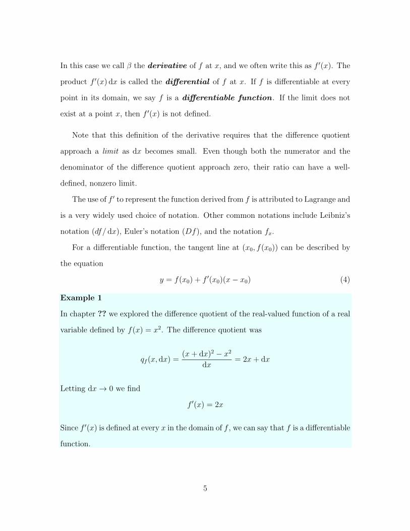
In this case we call β the derivative of f at x, and we often write this as f ′(x). The

product f ′(x) dx is called the differential of f at x. If f is differentiable at every

point in its domain, we say f is a differentiable function . If the limit does not

exist at a point x, then f ′(x) is not defined.

Note that this definition of the derivative requires that the difference quotient

approach a limit as dx becomes small. Even though both the numerator and the

denominator of the difference quotient approach zero, their ratio can have a well-

defined, nonzero limit.

The use of f ′ to represent the function derived from f is attributed to Lagrange and

is a very widely used choice of notation. Other common notations include Leibniz’s

notation (df/ dx), Euler’s notation (Df), and the notation fx.

For a differentiable function, the tangent line at (x0, f(x0)) can be described by

the equation

y = f(x0) + f ′(x0)(x− x0) (4)

Example 1

In chapter ?? we explored the difference quotient of the real-valued function of a real

variable defined by f(x) = x2. The difference quotient was

qf (x, dx) =(x+ dx)2 − x2

dx= 2x+ dx

Letting dx→ 0 we find

f ′(x) = 2x

Since f ′(x) is defined at every x in the domain of f , we can say that f is a differentiable

function.

5

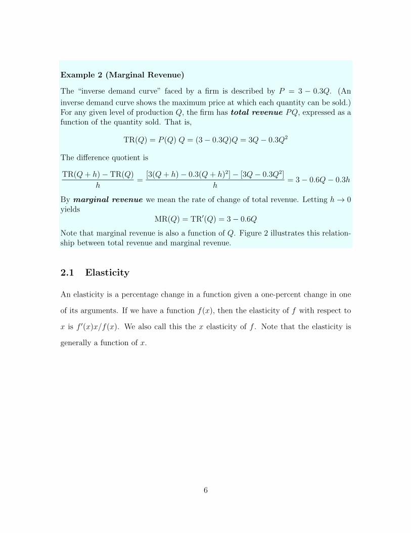
Example 2 (Marginal Revenue)

The “inverse demand curve” faced by a firm is described by P = 3 − 0.3Q. (An

inverse demand curve shows the maximum price at which each quantity can be sold.)For any given level of production Q, the firm has total revenue PQ, expressed as afunction of the quantity sold. That is,

TR(Q) = P (Q) Q = (3− 0.3Q)Q = 3Q− 0.3Q2

The difference quotient is

TR(Q+ h)− TR(Q)

h=

[3(Q+ h)− 0.3(Q+ h)2]− [3Q− 0.3Q2]

h= 3− 0.6Q− 0.3h

By marginal revenue we mean the rate of change of total revenue. Letting h→ 0yields

MR(Q) = TR′(Q) = 3− 0.6Q

Note that marginal revenue is also a function of Q. Figure 2 illustrates this relation-ship between total revenue and marginal revenue.

2.1 Elasticity

An elasticity is a percentage change in a function given a one-percent change in one

of its arguments. If we have a function f(x), then the elasticity of f with respect to

x is f ′(x)x/f(x). We also call this the x elasticity of f . Note that the elasticity is

generally a function of x.

6

−4

−2

0

2

4

0 2 4 6 8 10

0

2

4

6

8

10

Figure 2: Total Revenue and Marginal Revenue

7

Example 3 (MR and Elasticity)

Recall that if the demand curve Q(P ) can be represented by an inverse function P (Q),

then total revenue can be written as TR(Q) = QP (Q) and marginal revenue is

MR(Q) = P (Q) +QP ′(Q) = P (Q)

(1 + P ′(Q)

Q

P (Q)

)

This tells us that when a firm faces a downward sloping demand curve, it’s marginal

revenue depends not only on the current price but also on the responsiveness of

price to changes in the quantity supplied. That responsiveness is represented by the

elasticity term.

Since the slope of the inverse function is the inverse of the slope of the function,

the elasticity of the inverse function is also the inverse of the elasticity of the function.

So it is popular to rewrite this relationship as

MR = P (1 + 1/ε)

where ε is the price elasticity of demand.

Exercise 1

Suppose that the quantity demanded of apples (Q) at each price (P ) can be repre-

sented by the equation

Q = 1500− 20P

What is the price elasticity of the demand for apples? At what quantity of apples

does marginal revenue become zero?

8

2.2 Difficulties

Sometimes there is no obvious way to determine a unique tangent line at a point.

Consider for example figure 3. At point x0 there are many possible tangents: the

function has a “kink” in it. Reflecting this, note that at x0 the value of the difference

function calculated for dx < 0 has no tendency to approach the value calculated for

dx > 0. At point x1 the function has a break: this discontinuity also introduces the

possibility of many different “tangents”. Again reflecting this, note that at x1 the

value of the difference quotient calculated for dx < 0 has no tendency to approach

the value calculated for dx > 0.

f(x0)

f(x1)

x1x0

Figure 3: Tangency Problems

Such kinks and breaks do have economic relevance. As a classic example, a stan-

dard model of oligopoly implies that each oligopolistic firm faces a kinked demand

curve. The implied total revenue curve is correspondingly kinked, and the marginal

revenue curve has a break in it. As another example, the US income tax code changes

the tax rate at discrete income levels. This means that the individual relationship

between income and taxes is not differentiable at those levels.

9

2.3 Differentials

Let f be a differentiable real-valued function of a real variable. We know that if f

is affine, the notion of a slope is unambiguous. The difference quotient for an affine

function is constant; it does not depend on x or dx. The change in value of the

function is in proportion to the change in the value of its arugment, where the factor

of proportionality is the constant difference quotient. That is, given an affine function

f(x) = a0 + a1x, we have

f(x+ dx)− f(x) = a1 dx (5)

where a1 is the constant value of the difference quotient.

When f is nonlinear, it does not have a constant slope, but f ′(x) represents its

slope at a particular point. Although we cannot expect to find a constant a1 such

that f(x+ dx)− f(x) = a1 dx without remainder, the derivative serves a similar role

in the limit. To see this, define the remainder by

r(x, dx)def= f(x+ dx)− [f(x) + f ′(x) dx] (6)

This breaks the actual change in the value of f into two pieces: the differential and

the remainder.

f(x+ dx)− f(x) = f ′(x) dx+ r(x, dx) (7)

Wherever a function is differentiable, the remainder approaches zero faster than dx

10

does, in the following sense:

limdx→0

r(x, dx)

dx= lim

dx→0

f(x+ dx)− [f(x) + f ′(x) dx]

dx

= limdx→0

[f(x+ dx)− f(x)]− f ′(x) dx

dx

= f ′(x)− f ′(x) = 0

(8)

For this reason, we say that the differential approximates the actual change in the

value of the function. Here is another way to think about this: when dx is small the

change along the tangent line is a good approximation of the actual change in the

value of the function.

Example 4

Suppose f(x) = 5x2 + 2. Note that

limdx→0

f(x+ dx)− f(x)

dx= lim

dx→0

10x dx+ 5 dx2

dx= lim

dx→010x+ 5 dx = 10x

That is, 10x is the derivative of f at x. Therefore the differential of f at x is f ′(x) dx.Now for any x and dx we have the actual change in the function is

f(x+ dx)− f(x) = 5(x2 + 2x dx+ dx2) + 2− (5x2 + 2)

= 10x dx+ 5 dx2

The differential is f ′(x) dx = 10x dx, and the remainder is r(x, dx) = 5 dx2. Examin-ing the remainder we find

limdx→0

r(x, dx)

dx= lim

dx→0

5 dx2

dx= lim

dx→05 dx = 0

Suppose x rises from 1.0 to 1.1, so that dx = 0.1. Then f(x) rises from 7.0 to 8.05, sothat f(x+ dx)− f(x) = 1.05. The differential approximation is f ′(x) dx = 10 · 0.1 =1.00, which is close to the true change.

11

2.3.1 Predicting Change

Suppose you are given f ′(x) and you are asked to predict the change in the value of

f given a change dx in the argument. Recalling (4), one obvious way is to use the

differential to get a linear approximation dy of the change.

dy = f ′(x0) dx (9)

This will be perfect if f is linear.

If f is nonlinear, we might be able to do better. For example, if f is concave

we know that our predicted change will too large or too small as f ′(x0) is positive

or negative. And if f is convex we know that our predicted change will too large

or too small as f ′(x0) is negative or positive. One way to offset such effects of the

functions curvature on our prediction would be to use the average of the slopes at x0

and x0 + dx.

dy =f ′(x0) + f ′(x0 + dx)

2dx (10)

Example 5

Consider the function defined by f(x) = x2, with x0 = 2 and dx = 1. The true

change in the function is f(3) − f(2) = 9− 4 = 5. Since f ′(x) = 2x, the differential

approximation is dy = f ′(2) · 1 = 4. Our modified differential approximation is

dy = 0.5(f ′(2) + f ′(3)) · 1 = 0.5(4 + 6) = 5.

Consider the function defined by f(x) = x3, with x0 = 2 and dx = 1. The true

change in the function is f(3)−f(2) = 27−8 = 19. Since f ′(x) = 3x2, the differential

approximation is dy = f ′(2) · 1 = 12. Our modified differential approximation is

dy = 0.5(f ′(2) + f ′(3)) · 1 = 0.5(12 + 27) = 19.5.

12

3 Numerical Derivatives

In this chapter we are learning to find explicit derivatives for many convenient func-

tional forms. However, many actual applications introduce functional forms that are

not analytically tractable. In this case, we may be forced to compute approximations

to the analytical derivatives.

Assume you have defined a function f(x) and have picked a value for dx. As long as

dx is small in absolute value, the difference quotient qdx computes an approximation

to the analytical derivative at each x. In a computational setting, we refer to such

an approximation as a numerical derivative . A numerical derivative just the

computes slope of the function over a small but finite interval.

One obvious difficulty in computing a numerical derivative is that we cannot

literally consider dx → 0. Instead we are forced to make a choice of some small but

finite value for dx. Given the definition of the derivative, we might simply try to

make dx as small as possible.2 Instead we often keep things simple by choosing a

somewhat arbitrary small, fixed value for dx. (See section 3.1 for a more detailed

discussion.)

3.1 Forward Difference

Computational considerations affect our approach to numerical differentiation. Con-

sider the standard forward difference:

q(x, dx) =f(x+ dx)− f(x)

dxdx > 0 (11)

2This is not generally the best solution ?, p.280. We are working with computed rather thanactual values of f , which introduces some error. Let f(x) stand for the computed value of f(x).Suppose f(x) and f(x+ dx) can each be wrong by as much as ε in either direction. Then the truevalue of the slope from x to x+ dx can differ from the computed value by as much as 2ε/ dx. If wehave information on the curvature of f , we can use this to pick a best value for dx.

13

Based on the definition of the derivative, we might want to let dx get as small as pos-

sible. But if we use floating point arithmetic, which will be common when performing

such compuations on a computer, then past a certain point we will lose computational

accuracy by making dx smaller. (See section ?? for a taste of some of the intricacies

of floating point computations.)

Figure 4 illustrates this problem in the computation of the derivative of ex at

x = 1.3 (Here e is the “natural base,” also called “Euler’s number,” and is about

2.7.) The analytical derivative of ex is ex, which evaluates to e at x = 1. Since e is a

known value, we can readily compare our numerical results to the true answer. The

result of this comparison is displayed in figure 4, which shows that a smaller value for

dx is not always better. Such results are sometimes offered as a loose justification of

a rule of thumb: set dx =√εM |x|, where εM is the unit roundoff (i.e., the smallest

number such that 1 + ε > 1). ?, p.103 note that this rule needs to be modified for

small x, and they therefore propose dx =√εM max(|x|, 1). As a rough rule of thumb,

we will use dx = (1.5× 10−8) max(|x|, 1).4

We consider one final numerical issue for the accuracy of our forward difference

approximation to the derivative. It may seem reasonable analytically to define our

difference quotient as usual for computation:

q(x, h) =f(x+ h)− f(x)

h(12)

However, it is problematic numerically. Let xphdef= xfp + hfp be the computed sum

of the floating point representation of x and the floating point representation of h.

As we saw in table ??, However, with floating point numbers, we cannot assume

3See ?, p.103 and ?, p.322 for additional discussion of this example.4This assumes double-precision floating-point computation, since in this case

√εM ≈ 1.5× 10−8.

See computational exercise 5 for further exploration.

14

-16 -14 -12 -10 -8 -6 -4 -2 0

log10(dx)

-8

-6

-4

-2

0

log10(error)

Figure 4: Numerical Derivative of ex: Accuracy and dx

that hfp = (xfp + hfp) − xfp! (See section ??.) Since we want the denominator of

our difference quotient to be the distance between the input values for our function,

we may expect to more closely approximate the analytical difference quotient if we

compute our numerical derivative as follows:

q(x, h) =f(x+ h)− f(x)

(x+ h)− x (13)

Listing 1: Numerical Derivative

#i n p u t : f f u n c t i o n t o d i f f e r e n t i a t e

#i n p u t : x p o i n t o f d i f f e r e n t i a t i o n

#o u t p u t : computed d i f f e r e n c e q u o t i e n t

Function dfdx fwd ( f , x ) :#comment : r u l e o f thumb f o r dx

dxru le ← ( 1 . 5 · 10ˆ−8) ·max(1 ,abs ( x ) )#comment : compute change ( v a l u e o f f )

15

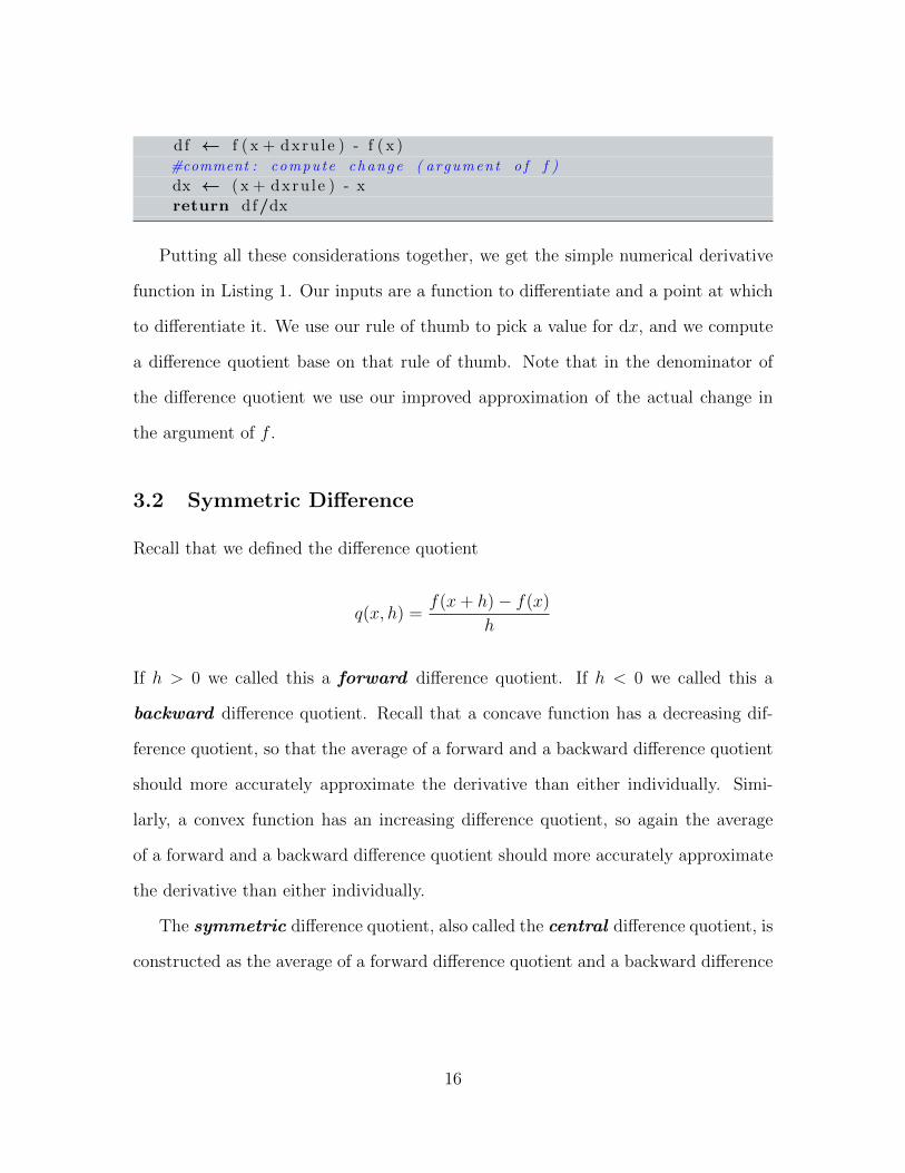
df ← f ( x + dxru le ) - f ( x )#comment : compute change ( argument o f f )

dx ← ( x + dxru le ) - xreturn df/dx

Putting all these considerations together, we get the simple numerical derivative

function in Listing 1. Our inputs are a function to differentiate and a point at which

to differentiate it. We use our rule of thumb to pick a value for dx, and we compute

a difference quotient base on that rule of thumb. Note that in the denominator of

the difference quotient we use our improved approximation of the actual change in

the argument of f .

3.2 Symmetric Difference

Recall that we defined the difference quotient

q(x, h) =f(x+ h)− f(x)

h

If h > 0 we called this a forward difference quotient. If h < 0 we called this a

backward difference quotient. Recall that a concave function has a decreasing dif-

ference quotient, so that the average of a forward and a backward difference quotient

should more accurately approximate the derivative than either individually. Simi-

larly, a convex function has an increasing difference quotient, so again the average

of a forward and a backward difference quotient should more accurately approximate

the derivative than either individually.

The symmetric difference quotient, also called the central difference quotient, is

constructed as the average of a forward difference quotient and a backward difference

16

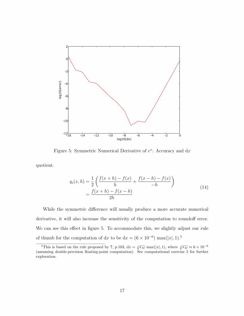
-16 -14 -12 -10 -8 -6 -4 -2 0

log10(dx)

-12

-10

-8

-6

-4

-2

0

2

log10(error)

Figure 5: Symmetric Numerical Derivative of ex: Accuracy and dx

quotient.

qs(x, h) =1

2

(f(x+ h)− f(x)

h+f(x− h)− f(x)

−h

)

=f(x+ h)− f(x− h)

2h

(14)

While the symmetric difference will usually produce a more accurate numerical

derivative, it will also increase the sensitivity of the computation to roundoff error.

We can see this effect in figure 5. To accommodate this, we slightly adjust our rule

of thumb for the computation of dx to be dx = (6× 10−6) max(|x|, 1).5

5This is based on the rule proposed by ?, p.103, dx = 3√εM max(|x|, 1), where 3

√εM ≈ 6× 10−6

(assuming double-precision floating-point computation). See computational exercise 5 for furtherexploration.

17

4 Some Rules of Differentiation

Constant rule f(x) = k =⇒ f ′(x) = 0 (where k is a constant).

This just says that a constant function has zero slope. For example, if f(x) = 5

then f ′(x) = 0.

Proof:

Given f(x) = k, at any x we have f(x+ dx)− f(x) = 0. So

limdx→0

f(x+ dx)− f(x)

dx= lim

dx→0

0

dx= 0 (15)

Scalar rule f(x) = kx =⇒ f ′(x) = k (where k is a constant).

This just says that a linear function has constant slope. For example, if f(x) = 5x

then f ′(x) = 5. Similarly, if f(x) = x then f ′(x) = 1.

Proof:

Given f(x) = kx, at any x we have

limdx→0

f(x+ dx)− f(x)

dx= lim

dx→0

k(x+ dx)− kxdx

= limdx→0

k dx

dx= k (16)

Additive inverse rule f = −g =⇒ f ′ = −g′

If a function has a positive slope (i.e., is rising in value), then its additive inverse

must have a negative slope (i.e., must fall in value). For example, if f(x) = −5x and

g(x) = 5x, we have f ′(x) = −5 = −g′(x).

Proof:

18

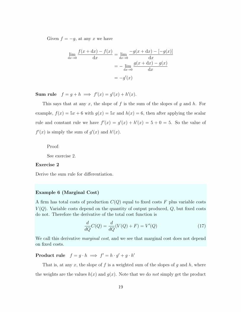
Given f = −g, at any x we have

limdx→0

f(x+ dx)− f(x)

dx= lim

dx→0

−g(x+ dx)− [−g(x)]

dx

= − limdx→0

g(x+ dx)− g(x)

dx

= −g′(x)

Sum rule f = g + h =⇒ f ′(x) = g′(x) + h′(x).

This says that at any x, the slope of f is the sum of the slopes of g and h. For

example, f(x) = 5x+ 6 with g(x) = 5x and h(x) = 6, then after applying the scalar

rule and constant rule we have f ′(x) = g′(x) + h′(x) = 5 + 0 = 5. So the value of

f ′(x) is simply the sum of g′(x) and h′(x).

Proof:

See exercise 2.

Exercise 2

Derive the sum rule for differentiation.

Example 6 (Marginal Cost)

A firm has total costs of production C(Q) equal to fixed costs F plus variable costs

V (Q). Variable costs depend on the quantity of output produced, Q, but fixed costsdo not. Therefore the derivative of the total cost function is

d

dQC(Q) =

d

dQ(V (Q) + F ) = V ′(Q) (17)

We call this derivative marginal cost, and we see that marginal cost does not dependon fixed costs.

Product rule f = g · h =⇒ f ′ = h · g′ + g · h′

That is, at any x, the slope of f is a weighted sum of the slopes of g and h, where

the weights are the values h(x) and g(x). Note that we do not simply get the product

19

of the derivatives. For example, if f(x) = x2 we can let g(x) = x and h(x) = x to

write f(x) = g(x)h(x), so that our rule implies f ′(x) = h(x) · g′(x) + g(x) · h′(x) =

x · 1 + x · 1 = 2x.

Proof:

There is one trick to this proof: the use of a well chosen zero. Given

f = gh, at any x we have

limdx→0

f(x+ dx)− f(x)

dx

= limdx→0

g(x+ dx)h(x+ dx)− g(x)h(x)

dx

= limdx→0

g(x+ dx)h(x+ dx)− g(x)h(x+ dx) + g(x)h(x+ dx)− g(x)h(x)

dx

= limdx→0

h(x+ dx)(g(x+ dx)− g(x)) + g(x)(h(x+ dx)− h(x))

dx

= limdx→0

h(x+ dx)g(x+ dx)− g(x)

dx+ lim

dx→0g(x)

h(x+ dx)− h(x)

dx

= h(x)g′(x) + g(x)h′(x)

(18)

Quotient rule f = 1/g =⇒ f ′(x) = −g′(x)/g(x)2

For example, f(x) = 1/x2 =⇒ f ′(x) = −2x/x4 = −2/x3

Comment: we can say intuitively that if f(x) = 1/g(x) then the growth rate of f

should be the inverse of the growth rate of g: that is, f ′(x)/f(x) = −g′(x)/g(x). But

this just means that f ′(x) = −f(x)g′(x)/g(x) = −g′(x)/g(x)2.

Comment: we often refer to the result that f(x) = h(x)/g(x) =⇒ f ′(x) =

[g(x)h′(x)− h(x)g′(x)]/g(x)2 as the quotient rule. You should show this follows from

our simple quotient rule and the product rule.

Proof:

20

Given f(x) = 1/g(x), at any x we have

limdx→0

f(x+ dx)− f(x)

dx= lim

dx→0

1/g(x+ dx)− 1/g(x)

dx

= limdx→0

g(x)− g(x+ dx)

g(x)g(x+ dx)

1

dx

= limdx→0

g(x)− g(x+ dx)

dx

1

g(x)g(x+ dx)

= − g′(x)

[g(x)]2

(19)

If we have f(x) = h(x)/g(x), we can apply the quotient rule along with the

product rule to conclude

f ′(x) = h′(x)/g(x)− g′(x)

[g(x)]2h(x) =

h′(x)g(x)− g′(x)h(x)

[g(x)]2(20)

Example 7 (Marginal Cost and Average Cost)

Suppose we know the total cost of production as a function of the level of output

produced, so we know C(Q). The average cost of production must be AC(Q)def=

C(Q)/Q. Let us use the quotient rule to consider the slope of the average cost

function.

AC′(Q) =d

dQ

C(Q)

Q

=C ′(Q)Q− C(Q)

Q2

=1

Q

(C ′(Q)− C(Q)

Q

)

=1

Q(C ′(Q)− AC(Q))

(21)

That is, the average cost curve is rising when marginal cost is above average cost,

and it is falling when marginal cost is below average cost.

21

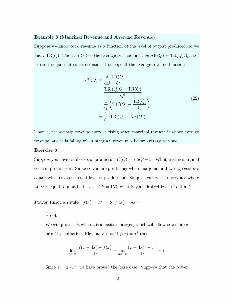
Example 8 (Marginal Revenue and Average Revenue)

Suppose we know total revenue as a function of the level of output produced, so we

know TR(Q). Then for Q > 0 the average revenue must be AR(Q) = TR(Q)/Q. Let

us use the quotient rule to consider the slope of the average revenue function.

AR′(Q) =d

dQ

TR(Q)

Q

=TR′(Q)Q− TR(Q)

Q2

=1

Q

(TR′(Q)− TR(Q)

Q

)

=1

Q(TR′(Q)− AR(Q))

(22)

That is, the average revenue curve is rising when marginal revenue is above average

revenue, and it is falling when marginal revenue is below average revenue.

Exercise 3

Suppose you have total costs of production C(Q) = 7.5Q2+15. What are the marginal

costs of production? Suppose you are producing where marginal and average cost are

equal: what is your current level of production? Suppose you wish to produce where

price is equal to marginal cost. If P = 150, what is your desired level of output?

Power function rule f(x) = xn =⇒ f ′(x) = nxn−1

Proof:

We will prove this when n is a positive integer, which will allow us a simple

proof by induction. First note that if f(x) = x1 then

limdx→0

f(x+ dx)− f(x)

dx= lim

dx→0

(x+ dx)1 − x1dx

= 1

Since 1 = 1 · x0, we have proved the base case. Suppose that the power

22

function rule holds for n− 1:

d

dxxn−1 = (n− 1)xn−2

Then we can apply the product rule to conclude

d

dxxn =

d

dx(xxn−1) = xn−1 + (n− 1)xn−2x = nxn−1

So by induction, the power rule is valid for any positive integer n. Now

suppose for some positive integer n we have f(x) = x−n, where we define

x−n = 1/xn for x 6= 0. Applying the quotient rule, we have f ′(x) =

−nxn−1/x2n = −nx−n−1, so we can apply the power function rule to any

integer n. (In fact on the domain of positive real numbers, we can apply

the power rule for real number n. but we will not prove that here.)

Other rules We offer these without proof for now.

� Inverse Function: (f−1)′ = 1/f ′.

� Natural Base (e): f(x) = ln(x) =⇒ f ′(x) = 1/x and f(x) = ex =⇒ f ′(x) =

ex. (Note: since ex ≡ ∑∞k=0(x

k/k!), this result is expected from the power

function rule and the sum rule.)

� General Exponential: f(x) = bx =⇒ f ′(x) = ln(b) · bx, where b is an arbitrary

base. Similarly, f(x) = logb x =⇒ f ′(x) = 1/x ln b.

Observation on the general exponential:

Suppose f(x) = bx, where b is an arbitrary base. We can rewrite this as f(x) =

ex ln(b). Applying our rule for the natural base and the chain rule immediately implies

23

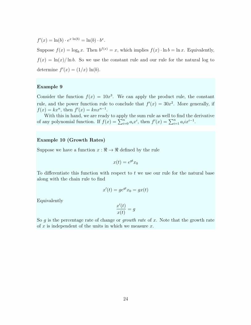
f ′(x) = ln(b) · ex ln(b) = ln(b) · bx.

Suppose f(x) = logb x. Then bf(x) = x, which implies f(x) · ln b = lnx. Equivalently,

f(x) = ln(x)/ ln b. So we use the constant rule and our rule for the natural log to

determine f ′(x) = (1/x) ln(b).

Example 9

Consider the function f(x) = 10x3. We can apply the product rule, the constant

rule, and the power function rule to conclude that f ′(x) = 30x2. More generally, iff(x) = kxn, then f ′(x) = knxn−1.

With this in hand, we are ready to apply the sum rule as well to find the derivativeof any polynomial function. If f(x) =

∑ni=0 aix

i, then f ′(x) =∑n

i=1 aiixi−1.

Example 10 (Growth Rates)

Suppose we have a function x : < → < defined by the rule

x(t) = egtx0

To differentiate this function with respect to t we use our rule for the natural basealong with the chain rule to find

x′(t) = gegtx0 = gx(t)

Equivalentlyx′(t)

x(t)= g

So g is the percentage rate of change or growth rate of x. Note that the growth rateof x is independent of the units in which we measure x.

24

Example 11 (Money Multiplier)

Define money as currency plus deposits (Mdef= C +D) and high-powered money to

be currency plus reserves (Hdef= C +R), so that the ratio of money to high-powered

money in the economy isM

H≡ C +D

C +R

If the currency-deposit ratio (cdef= C/D) and reserve-deposit ratio (r

def= R/D) are

constants, we can rewrite this as

M

H=c+ 1

c+ r

The term on the right is called the money multiplier. It is clear that a rise in thereserve-deposit ratio will reduce the money multiplier, but what about a rise in thecurrency-deposit ratio? A rise in c raises both the numerator and the denominator.If we think of the money multiplier as a function µ(c), then we can use the quotientrule and chain rule to find

µ′(c) =1 · (c+ r)− 1 · (c+ 1)

(c+ r)2=

r − 1

(c+ r)2< 0

So a rise in the currency-deposit ratio lowers the money multiplier as long as thereserve-deposit ratio is less than unity (which it is, of course).

Application (from Klein): Friedman and Schwartz note that at the beginningof the Great Depression in the US (Aug 1929–Mar 1933), H increased considerably(17.5%). However c and r rose fast enough to lead to a fall in the money supply byover a third. Monetary policy might have looked expansionary if we look at H, butnot if we look at M .

4.1 Function Composition and the Chain Rule

Given two functions f and g, the composition of f with g is denoted f ◦ g. Suppose

the real-valued functions f and g both have domain R. We can form a new function

h as the composition of f with g as follows: h(x)def= f(g(x)). We often represent

this new function by f ◦ g. So, using convenient notation, this new function can be

defined as

(f ◦ g)(x)def= f(g(x)) (23)

25

When we deal with functions whose domains are only a subset of the reals numbers,

we need to be a bit careful when thinking about the domain of the composition. The

domain of the composition is that part of the domain of g where the composition is

defined. For example, suppose f is defined on the reals while g is only defined on a

subset of the reals. (That is, f : R → R and g : X ⊂ R → R.) Then the domain of

the composed function is the domain of g.

When trying to understand a function—for example, when attempting to graph

it— it can be very helpful to notice that is can be written as a composition. Suppose

you notice that by completing the square

h(x) = ax2 + bx+ c (24)

can be written as f(g(x)) where g(x) = x + b/2a and f(x) = ax2 + (c − b2/4a).

Immediately you know the graph of h will be identical to the graph of ax2 except

translated. it will be translated horizontally by −b/2a units and vertically by c−b2/4a

units.

Example 12

Suppose

h(x) = x2 − 4x+ 4

Note that h(x) = f(g(x)) where g(x) = x − 2 and f(x) = x2. This implies that

know the graph of h will be identical to the graph of f with one exception: it will be

translated rightward by 2.

Chain rule: f = g ◦ h =⇒ f ′(x) = g′(y)h′(x) where y = h(x).

E.g., suppose f(x) = g(h(x)) where g(y) = 3y2 and h(x) = 2x+ 5. Then f ′(x) =

g′(y)h′(x) = (6y)(2) = ([6 · (2x+ 5)](2) = 24x+ 60.

26

5 Higher Order Derivatives

We have learned how to move from a given function to its derivative function. For

example, if we begin with a function f(x), then we defined value of its derivative

function f ′(x) at any x to be

limdx→0

f(x+ dx)− f(x)

dx(25)

But the derivative function is again a function, so we may be able to differentiate

it as well. If we refer to f ′(x) as the first-order derivative of f(x), then we can also

refer to the derivative of f ′(x) as the second-order derivative of f(x). We write this

as d2x/ dx2 or f ′′(x).

Example 13

Consider the function f defined by the rule f(x) = x4. Find the first, second, third,

and fourth-order derivatives of f(x).

f ′(x) = 4x3 f ′′(x) = 12x2 f ′′′(x) = 24x f ′′′′(x) = 24

Example 14

Consider the function defined by the rule f(x) = 1/x. Find the first, second, third,

and fourth-order derivatives of f .

f ′(x) = −x−2 f ′′(x) = 2x−3 f ′′′(x) = −6x−4 f ′′′′(x) = 24x−5

Exercise 4

Find the first, second, third, and fourth-order derivatives of f in the following cases.

f(x) = x4 + x3 + x2 + x+ 1 f(x) = ex f(x) = ln x f(x) = log10 x

27

If the derivative has an unambiguous sign, state it. If you can characterize the n-th

order derivative, do so.

5.1 Concavity and Convexity Redux

We have seen that the first-order derivative of a function f is also a function f ′,

which returns the slope of the primitive function for each value of the argument x. A

slope is a rate of change, so the derivative function tells us the rate of change of the

primitive function. For example, if f ′(x0) > 0, then we know that at x0 the value of

the function increases if we increase the argument.

Clearly the second-order derivative f ′′ will tell us the slope of the derivative func-

tion, so it is the rate of change of a rate of change. For example, if f ′′(x0) > 0, then

we know that at x0 the value of the derivative function increases if we increase the

argument, which means that the slope of the primitive function is increasing. The

second-order derivative is telling us about the curvature of the primitive function. So

a positive second-order derivative at x0 implies that the function is strictly convex at

x0. Similarly, a negative second-order derivative at x0 implies that the function is

strictly concave at x0.

28

Example 15 (Utility as a Function of Consumption)

Macroeconomic models often treat consumer utility as an increasing, concave function

of total consumption. That is, marginal utility is positive but declining. So a given

utility function u should at any consumption level c be characterized by u′(c) > 0

and u′′(c) < 0. Suppose we define u(c) =√c. Then u′(c) = 1/2

√c > 0 and

u′′(c) = −c−3/2/4 < 0. Suppose we define u(c) = ln c. Then u′(c) = 1/c > 0 and

u′′(c) = −1/c2 < 0. Suppose we define u(c) = −(c − c)2/2. Then u′(c) = c − c

and u′′(c) = −1 < 0. This last example only meets our requirements when c > c.

We might think of c as a “bliss” level of consumption that is not realized in actual

economies.

Exercise 5

Consider the general form of a quadratic polynomial: f(x) = a0 + a1x + a2x2, with

a2 6= 0. Is a quadratic polynomial concave or convex?

5.1.1 Inflection Points

Consider a twice differentiable function f . An inflection point x0 is a point where the

sign of f ′′ changes. That is, the function is concave on one side of x0 and convex on

the other side. If f is twice continuously differentiable, then f ′′(x0) = 0.

Example 16

The function defined by f(x) = x3 has as its second derivative f ′′(x) = 6x, so f is

concave to the left of 0 and convex to the right of 0. Note that although f ′(0) = 0,

we have an inflexion point, not an extremum, at x = 0. The function defined by

c(x) = x3− 3x2 + 5x+ 1 has a second derivative c′′(x) = 6x− 6, so c is concave to the

left of 1 and convex to the right of 1. Note that c′(1) = 2 > 0, so c is upward sloping

at this inflection point.

29

Problems for ReviewExercise 6

Let f1(x) = a0 + a1x and let f2(x) = a0 + a1x + a2x2. Calculate the difference

quotient for each function. Use your difference quotient to calculate the derivative

for each function.

Exercise 7

For each function below find f(x+ dx)− f(x), the differential, and the remainder for

any given dx.

� f(x) = 5

� f(x) = 2x+ 5

� f(x) = −7x2 + 2x+ 5

� f(x) = −7x2 + 2x

� f(x) = −7x2

In what sense are the remainders “small”?

Exercise 8

Age is often used as a proxy for experience in empirical work on compensation. Sup-

pose we find

w = 15 + 2A− 0.05A2

where w is the real wage and A is years of experience measured as years past age 15.

Find the wage at ages 20, 20, 40, 50, and 60. Find the value of a marginal year of

experience at each of those ages.

30

Exercise 9

Use the definition ∆f(x, dx) = f(x + dx) − f(x) and show all the algebra. Let

f(x) = a+ bx. Show that ∆f/ dx = b. Use the definition of ∆f given above. Derive

this result graphically.

Exercise 10

Use the definition ∆f(x, dx) = f(x + dx) − f(x) and show all the algebra. Let

f(x) = a+ bx+ cx2. Show that ∆f/ dx 6= b+ 2cx. Discuss how ∆f/ dx must behave

in order to serve as a good approximation to df/ dx, the derivative of f . What

determines the goodness of the approximation?

Exercise 11

Let f(x) = (5 − 3x)4. Find f ′(x) using the Chain Rule. Let f(x) = 12x3(6x − 2)5.

Find f ′(x) using the product rule and the Chain Rule. Let f(x) = (x2 + 5)/(x3).

Find f ′(x) using the quotient rule.

Exercise 12

For each function f below find f ′(x).

� f(x) = 5x+ 3

� f(x) = mx+ b

� f(x) = yx+ z

� f(x) = y2x+ z2

Be sure to show all your work and to explain which of the differentiation rules you

are using.

Exercise 13

For each function f below find f ′(x).

� f(x) = 5x2 + 3x+ 1

31

� f(x) = Ax2 +Bx+ C

� f(x) = px2 + qx+ r

Be sure to show all your work and to explain which of the differentiation rules you

are using.

Exercise 14

For each function f below find f ′(x).

� f(x) = 5(x+ 3)(x− 2)

� f(x) = A(x− x1)(x− x2)

� f(x) = 5(x− y)(x− z)

Be sure to show all your work and to explain which of the differentiation rules you

are using.

Exercise 15

Explain the difference between a power function and an exponential function. Explain

how to find the derivative of a power function. Give an example. Explain how to find

the derivative of an exponential function. Give an example.

Computational Exercises

Computational Exercise 1

Given a function f and two points x and x + h in the domain, we have learned to

calculate the difference quotient as q(x, h) = (f(x+h)−f(x))/h. Suppose f(x) = x2:

in example ?? we found analytically that limh→0 q(2, h) = 4. Now we will look at

this result graphically. Plot the difference quotient q(2, h) as h falls linearly from 1 to

0.01. Add your interpretation of the resulting plot in a program comment. Are you

32

surprised by the shape of your plot? Add a comment explaining the precise shape of

the resulting plot.

Computational Exercise 2

This problem illustrates some intricacies of computer arithmetic. Create functions

f and g such that f(x) = |x| and g(x) = x2. Create functions q1f and q1g that

produce the standard difference quotient for f and g. (These functions should take a

single argument: the point for evaluation. Set dx = 10−9 as a local variable.)

You are ready to produce numerical derivatives: evaluate your difference quotients

at three values: x = −2, 0, 2. Comment on your results by comparing them to

the analytic results. Now for something a bit surprising. Create slightly different

functions, q2f and q2g, which compute the “same” difference quotient with a slightly

different expression in the denominator: ((x+ dx)− x) instead of just dx. Use these

to again compute numerical derivatives at x = −2, 0, 2. Comment on any differences,

and speculate on the cause.

[Hint: how does your computer store x+ dx?]

Comment: As a more sophisticated variant of this exercise, instead of creating a

numerical derivative for each function, you may create a numerical derivative that

takes two arguments: a function and a point for evaluation.

Computational Exercise 3

Let f(x) = x2. and plot this function along with its numerical derivative. (Set

dx = 10−9.) Put the two plots in a single graph, and plot over the subdomain

[−2, 2]. In a program comment, explain the relation between the two plots. Next

let f(x) = |x|. Again plot this function along with its numerical derivative over the

subdomain [−2, 2]. In a program comment, explain the relation between the two

plots. Does the new function introduce any new considerations?

33

Supplementary Reading

?, ch.6–7.

34

6 Differentiability

Let f : X → < where X ⊂ <n is open. Then f is differentiable at x0 if we can find

a ∈ <n such that

lim‖ dx‖→0

f(x0 + dx)− f(x0)− a> dx

‖ dx‖ = 0 (26)

The row vector a> is called the derivative of f at x0, which we denote f ′(x0). It is

also called the gradient of f at x0. We call f ′(x0) dx the differential of f at x0. If f

is differentiable at every point of X then we say f is differentiable.

7 Application

Edwards p.70

Consider the differentiable function f : <n → < and a point x0 ∈ <n, where

f ′(x0) 6= 0. Let us determine the ‘direction’ in which f increases most rapidly. That

is, find a unit vector u that gives the direction of most rapid increase in the function.

As a preliminary, define the angle, θ, between x, y ∈ <N , x, y 6= 0, by

cos θ = x>y/‖x‖‖y‖ (27)

The change in the value of the function is approximated by f ′(x0) · u. Let θu

denote the angle between u and x0. Note

f ′(x0) · u = ‖f ′(x0)‖ cos θu (28)

Recall cos θu reaches a maximum at +1 when θu = 0, which means that u and f ′(x0)

are collinear and point in the same direction. The gradient gives the direction of most

rapid increase in the function.

35

Computational Exercise 4

Khamsi and Knaust offer the following example of a function f with inflection point

x0 where f ′′(x0) does not exist. Define a function f such that f(x) = x9/5− x, which

is continuous and differentiable. Graph the function, its derivative, and its second

derivative, and discuss the nature of the inflection point.

Computational Exercise 5

Try to produce error plots resembling figure 4 for the following functions: f(x) = x2,

f(x) = 1/x, f(x) = ln(x). (Evaluate each numerical derivative at x = 1.) Comment

on any problems in creating such plots, and when you can create a plot comment on

its similarities and differences from figure 4.

Computational Exercise 6

Modify the simple numerical derivative function in listing 1 to produce a numerical

derivative based on a symmetric difference quotient. Use this to plot the numerical

derivative of ex for x ∈ [0, 3]. Plot the analytical derivative as well, and compare the

two plots.

Computational Exercise 7

You work for a small cement plant. This plant currently produces about one ton of

cement each day. In response to a request from management, you have estimated daily

costs of production (in thousands of dollars per ton) to be C(Q) = Q3−3Q2 +5Q+1.

This expression means little to management, so graph total cost, average cost, and

marginal cost (in a single graph) that you will use in a presentation. (So make

your graph look beautiful.) If the market price is $1000/ton, what is your advice to

management? If the market price is $2000/ton, what is your advice to management?

If the market price is $4000/ton, what is your advice to management?

36

7.1 Differentiability Implies Continuity

Consider the behavior of any function f : < → < on an open interval I ⊆ <. If f is

differentiable at x ∈ I, then f is continuous at x.

Proof:

Consider

limdx→0

f(x+ dx)− f(x) = limdx→0

f(x+ dx)− f(x)

dxdx = f ′(x) · 0 = 0 (29)

That is

limdx→0

f(x+ dx) = f(x) (30)

37

Economic Models

Nonlinear Comparative Statics:First Approach

187

1 Non-linear IS-LM Comparative Statics

A model is more than a collection of structural equations: it is also a specification

of the endogenous variables. For example, suppose (1) and (2) are the “structual”

equations of a model.

Y = A(i− π, Y, F ) (1)

m = L(i, Y ) (2)

Here Y is total production in the economy, A is the function determining demand

for that production, i is the nominal interest rate, π is the expected inflation rate, F

measures the “fiscal stance” (i.e., how expansionary fiscal policy is), and m is the real

money supply. Equation (1) is an IS equation: it describes goods market equilibrium.

Total production in the economy must equal the total demand for that production.

Equation (2) is an LM equation: it describes money market equilibrium. The real

money supply in the economy must equal real money demand in the economy.

Refer to these equations as the “structural” equations, without worrying too much

about the nature of economic structure. These two structural equations can be used

to generate various models. E.g., produce a textbook “Keynesian” model by taking

Y and i to be the endogenous variables, or produce a textbook “Classical” model by

taking m and i to be the endogenous variables.

First, consider the textbook Keynesian model. Assuming satisfaction of the as-

sumptions of the implicit function theorem, there is an implied reduced form for

the Keynesian model. The reduced form expresses the solution for each endogenous

1

variables in terms of the exogenous variables. Represent this as

i = i(m,π, F ) (3)

Y = Y (m,π, F ) (4)

Note the conventional use the letter i to represent both a variable (on the left)

and a function (on the right). For blackboard algebra, this is common practice among

economists and mathematicians, as it helps us keep track of which function is related

to which variable. (Computer algebra usually requires us to adopt different symbols

for variable names and function names.) In the absence an explicit functional form

(e.g., linear) for the structural equations, there does not exist an explicit functional

form for the reduced form. Nevertheless, qualitative information about the structural

equations can imply qualitative statements about the reduced form.

The implicit function theorem tells relates the partial derivatives of i(., .) and

Y (., .) to such qualitative structural information. It provides the conditions under

which the partial derivatives of the reduced form are functions of the partial deriva-

tives of the structural form. These conditions are sufficient to investigate the quali-

tative comparative statics of the sturctural model.

First consider the money market. Recall that equation (2) described money mar-

ket equilibrium as

m = L(i, Y )

Suppose a money market that is in equilibrium experiences an exogenous change

and returns to equilibrium. The equation (2) must hold both before and after any

exogenous changes. That is, there is equilibrium in the money market before the

change, and there is equilibrium in the money market after the change. It follows

2

that any change in the real money supply (dm) must equal any change in real money

demand (dL). Represent the change in m as dm and the change in L as dL. Then

dm = dL (5)

Money demand depends on the value of its arguments. This implies that there

are two possible sources of change in money demand: a changes in i, and/or a change

in Y . As usual, represent these as di and dY . However, the change in real money

demand depends not only on the size of the changes in these arguments, but also

on how sensitive money demand is to each argument. Represent these sensitivities

as Li and LY . (This is just an alternative notation for the partial derivatives.) The

total change in money demand is the sensitivity-weighted sum of the changes in its

arguments.

dL = Li di+ LY dY (6)

Recall that (5) displays how the changes in m must relate to the changes in L if

the system is to both begin and end in equilibrium. Therefore, in light of (5),

dm = Li di+ LY dY (7)

Call equation (7) the “total differential” of the LM equation (2). It makes a very

simple statement: in order to start out in equilibrium and then end up in equilibrium,

any changes in m must equal the change in L.

The total differential can be used to find the slope of the LM curve. Suppose we

3

i

Y

LM

dY

di

Figure 1: Slope of LM Curve

allow only i and Y to change (so that dm = 0). Then we must have

0 = Lidi+ LY dY (8)

di

dY

∣∣∣∣LM

= −LY

Li

> 0 (9)

This represents the way i and Y must change together to maintain equilibrium in the

money market, ceteris paribus. That is, this determines the slope of the “Keynesian”

LM curve. Under the standard assumptions that LY > 0 and Li < 0, the “Keynesian”

LM curve has a positive slope.

Next consider the goods market. Recall that the equation

Y = A(i− π, Y, F ) (1)

4

represents equilibrium in the goods market. This must hold both before and after any

exogenous changes. That is, we require that we start out in goods market equilibrium,

and we also require that we end up in goods market equilibrium. It follows that the

changes in real income must equal the changes in real aggregate demand. Looking

at the equation for the IS curve, we can see that this means that the change in real

income (dY ) must equal the change in real aggregate demand (dA).

dY = dA (10)

The change in aggregate demand has three sources: changes in r, changes in Y , and

changes in F . We represent these changes as dr, dY , and dF . Of course, the changes

in aggregate demand depend not only on the size of the changes in these arguments,

but also on how sensitive aggregate demand is to each of these arguments.

dA = Ar

dr︷ ︸︸ ︷(di− dπ) +AY dY + AFdF (11)

Putting these two pieces together, we have the total differential of the IS equation:

dY = Ar(di− dπ) + AY dY + AFdF (12)

Note that A(·, ·, ·) has only three arguments. Do not be misled by the fact that

we choose to write r as i− π. This does not change the number of arguments of the

aggregate demand function. E.g., there is no derivative Ai. We may notice that if we

5

i

Y

IS

di

dY

Figure 2: Slope of IS Curve

allow only i and Y to change, we must have

dY = Ardi+ AY dY (13)

di

dY

∣∣∣∣IS

=1− AY

Ar

< 0 (14)

This is the way i and Y must change together to maintain equilibrium in the goods

market. That is, this determines the slope of the “Keynesian” IS curve. Under the

standard assumptions that 0 < AY < 1 and Ar < 0, the ”Keynesian” IS curve has a

negative slope.

So we have seen what is required to stay on the IS curve and what is required to

6

stay on the LM curve. Putting these together we have

dY = Ar(di− dπ) + AY dY + AFdF (15)

dm = Lidi+ LY dY (16)

When we insist that both of these equation hold together, we are insisting that

we stay on both the IS and LM curves simultaneously. In this system there are two

endogenous variables, dr and dY , which are being determined so as to achieve this

simultaneous satisfaction of the IS and LM equations.

Well, you know how to solve two linear equations in two unknowns. First prepare

to set up the system as a matrix equation by moving all terms involving the endoge-

nous variables to the left. (Note that this is the first time we have paid attention to

which variables are endogenous.)

−Ardi+ dY − AY dY = −Ardπ + AFdF (17)

Lidi+ LY dY = dm (18)

Now rewrite this system as a matrix equation in the form Jx = b.

−Ar (1− AY )

Li LY

di

dY

=

−Ardπ + AFdF

dm

(19)

7

Then solve for the endogenous variables by multiplying both sides by J−1.

di

dY

=

1

−ArLY − (1− AY )Li

LY −(1− AY )

−Li −Ar

−Ardπ + AFdF

dm

=1

ArLY + (1− AY )Li

−LY (1− AY )

Li Ar

−Ardπ + AFdF

dm

(20)

Letting ∆ = ArLY + (1− AY )Li, we can write this as

di

dY

=

1

∆

−LY (1− AY )

Li Ar

−Ardπ + AFdF

dm

(21)

Notice that ∆ < 0.

We know from the implicit function theorem that this is the same as solving for

the partial derivatives of the reduced form. Invoking the standard assumptions on

the structural form partial derivatives, listed above, we note that ∆ = ArLY + (1 −

AY )Li < 0, we can write

∂i/∂m

∂Y/∂m

=

1

∆

−LY (1− AY )

Li Ar

0

1

=1

∆

(1− AY )

Ar

=

−

+

(22)

8

∂i/∂π

∂Y/∂π

=

1

∆

−LY (1− AY )

Li Ar

−Ar

0

=1

∆

LYAr

−LiAr

=

+

+

(23)

∂i/∂F

∂Y/∂F

=

1

∆

−LY (1− AY )

Li Ar

AF

0

=1

∆

−LYAF

LiAF

=

+

+

(24)

In the Classical case we follow the same procedures and the same type of reasoning,

making only a single change: instead of Y we take m to be endogenous, so that m and

i are the endogenous variables. Note that we start with the same system of structural

equations:

Y = A(i− π, Y, F ) (25)

m = L(i, Y ) (26)

It follows that the total differential is unchanged:

dY = Ar(di− dπ) + AY dY + AF dF (27)

dm = Li di+ LY dY (28)

9

Of course, all the partial derivatives from the structural form are unchanged: Ar < 0,

0 < AY < 1, AF > 0, Li < 0, and LY > 0.

But of course we have a different set of endogenous variables, so we have a different

implied reduced form:

m = m(Y, π, F ) (29)

i = i(Y, π, F ) (30)

Since the set of endogenous variables has changes, we will rewrite our total differ-

ential to reflect the new set.

Ar di = Ar dπ + (1− AY ) dY − AF dF (31)

−Li di+ dm = LY dY (32)

So when we write down the matrix equation, we use our new set of endogenous

variables: Ar 0

−Li 1

di

dm

=

Ardπ + (1− AY )dY − AFdF

LY dY

(33)

Solving for the changes in the endogenous variables:

di

dm

=

1

Ar

1 0

Li Ar

Ardπ + (1− AY )dY − AFdF

LY dY

(34)

10

So for example

∂i/∂π

∂m/∂π

=

1

Ar

1 0

Li Ar

Ar

0

=1

Ar

Ar

LiAr

=

+

−

(35)

11

Optimization: First Approach

199

Optimization is the search for a best choice. The quality of a choice is determined

by our objectives. Economists often consider objectives such as utility maximization,

cost minimization, or profit maximization. These are different ways that economic

actors seek the best possible outcomes: maximization and minimization are types of

optimization. Maxima and minima are the extreme values, or extrema , of a function.

This chapter develops some mathematical tools for characterizing extrema.

1 Extrema

The basic maximization problem can be represented as

maxx∈F

f(x,θ) (1)

The function f is our objective function, whose value we are trying to maximize

by picking the best input x from the feasible set F. We are explicitly including

the parameter θ in the function, because we are often interested in how changes in

certain parameters affect the optimum. For example, we may be interested in how

a consumer responds to a change in wealth or how a producer responds to a price

change. Of course not all functions can be maximized. Recall that in section ?? we

classified functions according to whether or not they have extrema. We found that

any continuous function will reach a minimum and a maximum on a compact set.

In this section, we try to associate those extrema with the “flat spots” of differ-

entiable functions. That is, we look for values of x where the function f ′(x) = 0.

Any such x is called a stationary point of the function. A critical point of the

function is a stationary point or a point where the function is not differentiable.

Figure 1 illustrates some problems with the strategy of associating stationary

1

points with extrema. We have drawn the values of the function f over its feasible set.

Points B and E are local maxima. (Some authors prefer the term relative maximum.)

Point B is also a global maximum. (Some authors prefer the term absolute maximum.)

The derivative cannot be said to be zero at point B because the function is not

differentiable there. Point C is a local minimum, but point A (at the edge of the

feasible set) is the global minimum. Point D is a flat spot, but it is neither a minimum

nor a maximum.

Several points are illustrated by this figure. First, a local extremum need not

be a global extremum. In fact, many functions do not have a global maximum or

minimum. Second, a function may be “flat” (i.e., may have a zero first derivative)

at points other than minima and maxima. And finally, an extremum will only be

associated with a zero first derivative if the function is differentiable at that point

(i.e., the function must not jump or be kinked).

A

B

C

E

D

x

f(x)

Figure 1: Extrema: Local and Global

2

2 Derivatives and Optima

Looking at figure 1, we see that when we can speak of the slope of the function at

an interior local maximum, the slope is zero. (We will talk about maxima that are

boundary points a little later.) However we also see that when we can speak of the

slope of the function at an interior local minimum, the slope is zero. So if a function

is differentiable everywhere, the zero first-order derivative at a point is a necessary

but not a sufficient condition for an extremum. We call this the first-order necessary

condition for an extremum.

2.1 First Order Conditions

We have seen intuitively that a necessary condition for an interior extremum of dif-

ferentiable function is that the first derivative be zero. Since this condition involves

the first derivative of the function, it is called the first-order necessary condition. We

now develop this condition is a bit more detail.

Theorem 1 (Fermat’s Theorem for Stationary Points)

Consider the behavior of a continuous real-valued function f over an open interval.

If x is a local extremum of f and f is differentiable at x, then f ′(x) = 0.

Proof:

Suppose x is a local maximizer of f . That is, there is a neighborhood

N(x) such that

f(x+ dx)− f(x) ≤ 0 ∀(x+ dx) ∈ N(x) (2)

3

This implies the difference quotient is always positive to the left of x, so

limdx→0−

f(x+ dx)− f(x)

dx≥ 0 (3)

It also implies the difference quotient is always negative just to the right

of x, so

limdx→0+

f(x+ dx)− f(x)

dx≤ 0 (4)

But f is differentiable, so these two limits must be equal. This is possible

only if f ′(x) = 0. We show this for the case of a local minimizer in the

same way.

2.2 Zeros

Given a function f , the values of x such that f(x) = 0 are called the zeros of f or

the roots of the equation f(x) = 0.

Example 1

Suppose we want to find the zeros of the function f defined by the rule f(x) = mx+b.

Setting mx+ b = 0 we find the unique zero is x = −b/m. We call this the x-intercept

of the graph of the function.

Economists often produce a collection of equations (called first order conditions)

for which they seek the roots as solutions to an optimization problem.

Suppose you have two functions f and g and you are interested in their points of

intersection. Equivalently, you are interested in any (x, y) shared by the two functions,

so that y = f(x) and y = g(x). Such points are called a solution to the equation

4

system

y = f(x) (5)

y = g(x) (6)

Graphically, you could plot the two equations and look for their intersection. Equiv-

alently, you could look for the zeros of f(x)− g(x).

2.3 Inflection Points and Stationary Points

Definition 2.1 Consider function f : X ⊆ < → <. A point x is an inflection point

of f if f is concave on one side of x and convex on the other side. If f is twice

differentiable, this means f ′′(x) = 0 and f ′′ changes sign at x.

Definition 2.2 We way that x is a stationary point of a function f if

f ′(x) = 0

We way that x is a critical point of f if it is a stationary point of f or if f ′(x) is not

defined.

Suppose we are considering an everywhere differentiable function f : < → <. At

a stationary point, the value of f is neither increasing nor decreasing. The slope is

zero. Three possible cases cases immediately present themselves.

1. on either side of x we have f(x) ≤ f(x), so x is a local maximizer.

2. on either side of x we have f(x) ≥ f(x), so x is a local minimizer.

3. on one side of x we have f(x) < f(x), while on the other side of x we have

5

f(x) > f(x), so x is neither a local maximizer nor a local minimizer. In this

case x must be an inflection point.

This suggests that in trying to characterize an optimum we will need more information

than its slope. If we find a stationary point, we still need to know something about

nearby values. We might get this information by looking directly at nearby values of

the function. We might get this information by looking at nearby values of f ′. Or we

might examine the curvature of our objective function near the stationary point.

2.4 Curvature

Our first order necessary condition describes extrema and horizontal inflection points.

To be confident of being at a maximum or a minimum, we need more information.

For a local maximum, we additionally need the nearby values of the function to be

smaller. For a local minimum, we additionally need the nearby values of the function

to be larger. If we find a critical point, then we can try to verify that near the critical

value the function always takes on smaller (or larger) values. This would be sufficient

information to conclude that we have a local maximum (or minimum).

When our function is adequately differentiable, we can seek this extra information

in the second-order derivative. Recall that the second-order derivative tells us about

the curvature of the function. If a function is strictly-concave at a critical point, then

we have found a local maximum. If a function is strictly-convex at a critical point,

then we have found a local minimum.

6

Example 2

Suppose f(x) = x2, so that f ′(x) = 2x and f ′′(x) = 2. We see that a critical point

can be found at x = 0. Since f ′′(0) = 2 > 0, the function is convex near the critical

point and we have therefore found a local minimum. (In fact, the function is globally

convex, so we have found a global minimum.)

Suppose f(x) = x3, so that f ′(x) = 3x2 and f ′′(x) = 6x. We see that a critical

point can be found at x = 0. Since f ′′(0) = 0, the second-order condition does not

suggest that the function is concave or convex near the critical point. And in fact,

we have therefore found an inflection point.

Example 3 (Laffer Curve)

Consider the tax-revenue function f : [0, 1]→ <+ defined by the rule f(t) = θ(t− t2),

with θ > 0. Here t is the tax rate and θ is an economy specific parameter determining

total tax revenues at each tax rate. We want to determine the revenue maximizing

tax rate. We find f ′(t) = θ(1−2t), which allows us to can characterize the stationary

point by

1− 2t = 0

or t = 0.5. Since f ′′(t) = −2θ we know the function is concave, so we have found a

maximizer.

Example 4

Let TC(Q) be the total cost function of a firm. Then MC(Q) = TC′(Q) is the marginal

cost function and AC(Q) = TC(Q)/Q is the average cost function. Suppose the firm

minimizes the average cost of production. Then it produces where AC′(Q) = 0,

so that TC′(Q)/Q − TC(Q)/Q2 = 0. Multiplying by Q and rearranging, we get

TC′(Q) = TC(Q)/Q or, equivalently, MC(Q) = AC(Q).

7

Example 5

The general maxim in economics is that any activity should be undertaken at the level

where marginal benefits equal marginal costs. We now apply this to profit maximiza-

tion, where the marginal benefit of an increase in production is the marginal revenue

derived from that production. Profits are the difference between total revenues and

total costs.

π(Q) = TR(Q)− TC(Q)

The first-order necessary condition for profit maximization, that π′ = 0, is therefore

characterized as

TR′(Q)− TC′(Q) = 0 (7)

That is, marginal revenue should equal marginal costs. Graphically, this has two

ready interpretations. If we draw the TR(Q) and TC(Q) curves, we are looking for a

value of Q where they have the same slope. If we draw the MR and MC curves, we

are looking for a value of Q where they cross.

Of course, this is a necessary not a sufficient condition for a maximum. It also

characterizes minima and inflections points. If we also find π′′ < 0, then we are

assured of a maximum. In this case

TR′′(Q)− TC′′(Q) < 0

at the critical point. This means that the slope of the TR curve should be less than

the slope of the TC curve, or equivalently that the MC curve should cut the MR

curve from below at the critical point.

Exercise 1

Consider a monopolist with constant marginal costs. Suppose the inverse demand

8

curve is

P = Q−1/β

where β > 0. Show that β is the elasticity of demand. Find the first order condition

for profit maximization. Demonstrate that satisfaction of the second order condition

depends on the value of β and suggest why.

Exercise 2

Suppose the monetary authority dislikes unemployment and really dislikes high in-

flation, as represented the the loss function L = U + π2. Here U is the difference

between the unemployment rate and the natural rate of unemployment, and π is the

inflation rate. The monetary authority picks the inflation rate to minimize its loss

function. We suppose U to be determined by U = 0.5(π − πe). (You may think of

this as a “Lucas supply curve”.) Here πe is expected inflation. Again, actual inflation

is the choice variable for the monetary authority. If the monetary authority treats

expected inflation as a fixed constant, what inflation rate will it set? If the monetary

authority treats expected inflation as always equal to actual inflation, what inflation

rate will it set?

Exercise 3

Anton et al. (2002) offer an example like the following. An oil well is located 6km

offshore. The refinery is located 8km further down the coast. Laying pipe costs

$1M/km under water and $0.5M/km over land. Propose the cheapest way to lay

pipe from the well to the refinery. (Assume the coast follows a straight line.)

To solve this, use the Pythagorean theorm to determine that the well is 10km

from the refinery across the water. (I.e.,√

62 + 82 = 10.) So building underwater

pipe straight to the refinery costs $10M. Alternatively you could minimize the amount

of underwater pipe at 6km for a total cost also of $10M. Is there no cheaper proposal?

9

2.5 Necessary Conditions for an Extremum

Recall that we found that a zero first-order derivative was a necessary condition for an

extremum. If this necessary condition is satisfied, we found that a non-zero second-

order derivative was sufficient for an extremum. But it is not necessary. We may

have a maximum or minimum at a critical point where the second-order derivative is

also zero. Such a point is called a degenerate critical point of f . In this section, we

explore the information provided about a degenerate critical point by higher order

derivatives.

Example 6

Consider the function f(x) = x4. We note that f ′(x) = 4x3 is zero at x = 0, but

f ′′(x) = 12x2 is also zero at x = 0. Nevertheless, x = 0 is the minimizer of the

function.

Let us use f (n)(x) to denote the nth-order derivative of f(x). Then if f ′(x0) = 0

and the first higher-order derivative that is non-zero at x0 is f (n)(x0), then we have

� an inflection point if n is odd

� a maximum if n is even and f (n)(x0) < 0

� a minimum if n is even and f (n)(x0) > 0

Generally, this will suffice for us determine whether a critical point is a maximizer,

a minimizer, or an inflection point. There are, however, odd functions with zero

derivatives of all orders at an extremum.

10

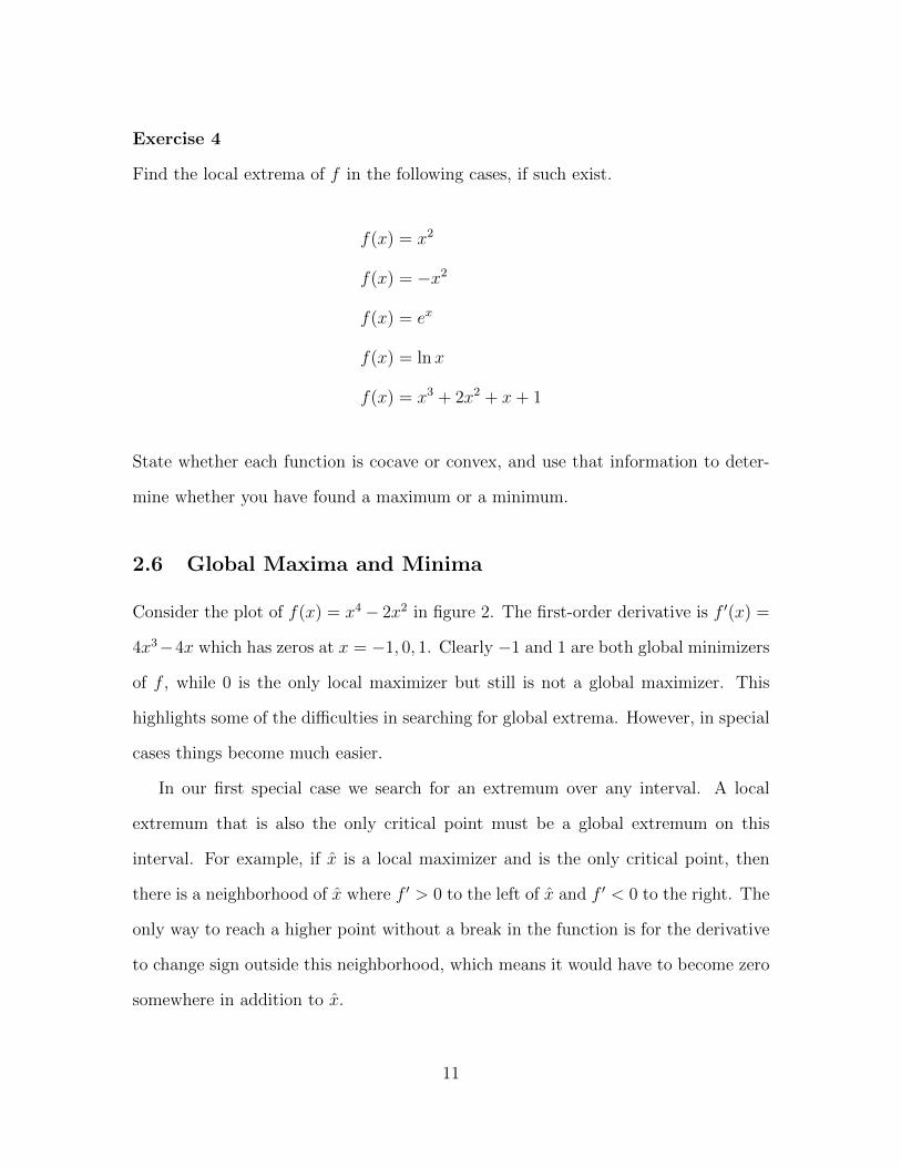
Exercise 4

Find the local extrema of f in the following cases, if such exist.

f(x) = x2

f(x) = −x2

f(x) = ex

f(x) = ln x

f(x) = x3 + 2x2 + x+ 1

State whether each function is cocave or convex, and use that information to deter-

mine whether you have found a maximum or a minimum.

2.6 Global Maxima and Minima

Consider the plot of f(x) = x4− 2x2 in figure 2. The first-order derivative is f ′(x) =

4x3−4x which has zeros at x = −1, 0, 1. Clearly −1 and 1 are both global minimizers

of f , while 0 is the only local maximizer but still is not a global maximizer. This

highlights some of the difficulties in searching for global extrema. However, in special

cases things become much easier.

In our first special case we search for an extremum over any interval. A local

extremum that is also the only critical point must be a global extremum on this

interval. For example, if x is a local maximizer and is the only critical point, then

there is a neighborhood of x where f ′ > 0 to the left of x and f ′ < 0 to the right. The

only way to reach a higher point without a break in the function is for the derivative

to change sign outside this neighborhood, which means it would have to become zero

somewhere in addition to x.

11

-2

-1.5

-1

-0.5

0

0.5

1

1.5

2

-2 -1.5 -1 -0.5 0 0.5 1 1.5 2

Figure 2: Critical Points: f(x) = x4 − 2x2

For the same reason, globally concave and globally convex functions can have at

most one extremum. We continue to focus on twice differentiable functions. Thinking

back to our discussion of local extrema, it is easy to guess that a globally concave

function will have at most one critical point, which must be a global maximizer (if

such exists).

In our second special case we search for an extremum over any compact (closed and

bounded) set in the domain. Weierstrass proved that a continuous function always

has a global maximum and a global minimum on such a set. This is obvious enough

when we consider a differentiable function f : < → < on a closed interval. Just check

the boundary values of the function, and compare them to the values at the critical

points, and pick the global extrema.

12

3 Equations

We have seen that for differentiable functions the search for interior extrema involves

a search for critical points. The first-order necessary condition is that f ′(x) = 0.

Since derivative functions are still just functions, we are involved in solving equations

of the form f ′(x) = 0. If these equations were linear, the problem would be simple.

Often however they are not linear. Thus our interest in critical points stimulates an

interest in general techniques for solving equations.

Suppose we want to solve an equation g(x) = 0. The roots are just the values of

x that satisfy this equation. (We can equivalently speak of the zeros of the function

g(x).) The number and type of roots depends on the equation. There may be no real

roots, a unique real root, or multiple real roots. There may also be complex roots,

but for now we will focus on real roots.

Some functions are easy to solve analytically for their zeros. Others are difficult or

even impossible. When the going gets tough, we may turn to graphical or numerical

approaches.

3.1 Ridders’s Method

Linear interpolation works quickly and perfectly for a linear function. For non-linear

functions, convergence can be slow. Ridders (1979) suggested linearizing the function

and then applying linear interpolation. The resulting algorithm is simple and robust,

with a good rate of convergence.

Here is how it works. Suppose we want to find a zero of f on a sign changing

interval [a, b]. We will construct a new function H(x) = emxf(x) such that (a +

d,H(a + d)) lies on the secant segment from (a,H(a)) to (b,H(b)). We will take

d = (b− a)/2, so that the midpoint of the segment is a point of H.

13

To accomplish this, we need H to rise (or fall) the same amount over each half

interval.

f(a+ 2d)em(a+2d) − f(a+ d)em(a+d) = f(a+ d)em(a+d) − f(a)ema (8)

which implies

f((a+ 2d)b)e2md − 2f(a+ d)emd − f(a) = 0 (9)

So we have produced a quadratic equation in emd. Solving using the quadratic formula

gives

emd =f(a+ d)±

√[f(a+ d)]2 − f(a)f(a+ 2d)

f(a+ 2d)(10)

Recall that we began with a sign changing interval, so f(a)f(a + 2d) < 0 and the

roots are real and of opposite sign. Note that we need emd > 0. Thus we have a

unique solution to our problem.

Scaling by f(a), we can rewrite our solution as

emd =f(a+ d)/f(a) +

√[f(a+ d)/f(a)]2 − f(a+ 2d)/f(a)

f(a+ 2d)/f(a)(11)

This is the scale factor used to produce H(x). The points (a,H(a)), (a+d,H(a+d)),

and (b,H(b)) lie on a straight line. Picking any two of these points, we can use linear

interpolation to approximate a zero of H.

Recalling our work on linear interpolation above, we set

x = xmid −H(xmid)b− xmid

H(b)−H(xmid)

= xmid −H(xmid)d

H(b)−H(xmid)

= xmid − dH(xmid)

H(b)−H(xmid)

(12)

14

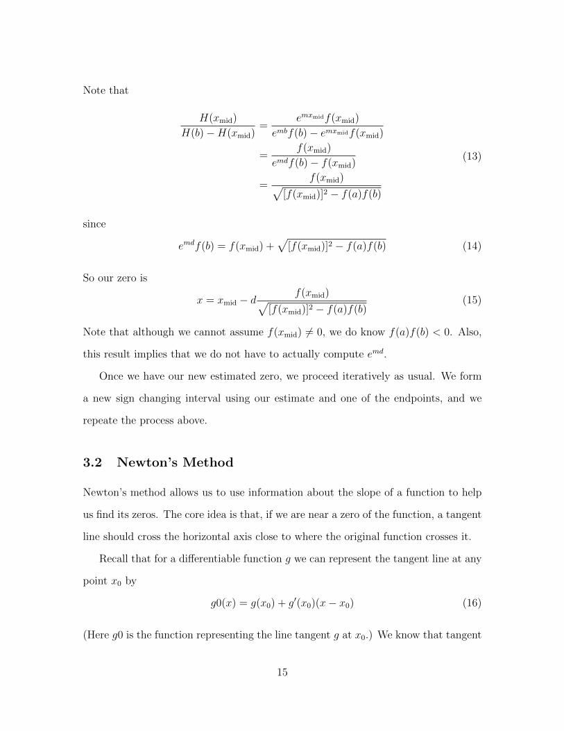
Note that

H(xmid)

H(b)−H(xmid)=

emxmidf(xmid)

embf(b)− emxmidf(xmid)

=f(xmid)

emdf(b)− f(xmid)

=f(xmid)√

[f(xmid)]2 − f(a)f(b)

(13)

since

emdf(b) = f(xmid) +√

[f(xmid)]2 − f(a)f(b) (14)

So our zero is

x = xmid − df(xmid)√

[f(xmid)]2 − f(a)f(b)(15)

Note that although we cannot assume f(xmid) 6= 0, we do know f(a)f(b) < 0. Also,

this result implies that we do not have to actually compute emd.

Once we have our new estimated zero, we proceed iteratively as usual. We form

a new sign changing interval using our estimate and one of the endpoints, and we

repeate the process above.

3.2 Newton’s Method

Newton’s method allows us to use information about the slope of a function to help

us find its zeros. The core idea is that, if we are near a zero of the function, a tangent

line should cross the horizontal axis close to where the original function crosses it.

Recall that for a differentiable function g we can represent the tangent line at any

point x0 by

g0(x) = g(x0) + g′(x0)(x− x0) (16)

(Here g0 is the function representing the line tangent g at x0.) We know that tangent

15

line lies near g(x) as long as x is near x0. Suppose we are trying to find x such that

g(x) = 0. As illustrated in figure 3, we will proceed as follows.

1. Begin with an initial guess at the value of x. In figure 3, we call this guess x0.

2. Find the tangent to the function g at the point(x0, g(x0)

). The tangent function

is g0(x) = g(x0)+g′(x0)(x−x0), so to find the tangent function we must compute

g(x0) and g′(x0).

3. Find the x-intercept of our tangent line. In figure 3, we call this x1. Since x1

is a zero of our tangent function, so that 0 = g(x0) + g′(x0)(x1 − x0), we find

x1 = x0 − g(x0)/g′(x0).

4. Now we have x1, our new, and hopefully improved, guess for x. So we can

repeat the entire: process: find the zero of the tangent to g at(x1, g(x1)

). (In

figure 3, we call this x2.)

5. We can repeat this process as long as we wish, producing a sequence (x0, x1, x2, . . . ),

where xn = xn−1 − g(xn−1)/g′(xn−1).

If our initial guess is close enough to x, then the tangent line and the graph of g will

still be close together as they each cross the x axis. That is, when g0(x) = 0 we

should be zero close to x. So let us take the solution of g0(x) = 0 as our improved

guess of a solution of g(x) = 0.

Finding the zero of a linear function is easy. We know the slope and the value

of the function at the initial point x0, so we just want to find x1 such that 0 =

g(x0) + g′(x0)(x1 − x0). That is, x1 = x0 − g(x0)g′(x0)

. We can now iterate using the

recursion relation

xn = xn−1 −g(xn−1)

g′(xn−1)(17)

16

g(x0)

0

g(x1)

x0 x2 x1

Figure 3: Newton’s Method

Equation (17) is called the Newton iteration formula.

How many times should we iterate? We would like to continue until we are close

enough to our desired answer, and this forces us to be explicit about what we will

mean by ‘close enough’. We must supply a convergence criterion. Perhaps the most

obvious convergence criterion is that the changes in x become so small that we no

longer care about them. From any point xr, the change in x is dx = −g(xr)/g′(xr).

So we implement our convergence criterion as test the deviation of dx from zero.

Listing ?? illustrates a simple implementation of Newton’s method.1

1The method is also known as the Newton-Raphson method (Ypma, 1995).

17

Listing 1: Newton’s Method

#g o a l :

# f i n d r o o t o f f u n c t i o n

#i n p u t :

# f : f u n c t i o n

# Df : f u n c t i o n ( f i r s t d e r i v a t i v e o f ` f ` )

# x (float), i n i t i a l g u e s s o f r o o t v a l u e

#o u t p u t :

# f l o a t , r o o t o f f u n c t i o n

Function newton ( f , Df , x ) :# i n i t i a l i z e : `dx ` f o r n e x t Newton i t e r a t i o n

dx ← −f ( x )/Df ( x )#comment : w h i l e no t c o n v e r g e n t , i t e r a t e

while abs ( dx ) ≥ 1e−9:#a s s i g n : n e x t i t e r a t e t o `x `

x ← x + dx#a s s i g n : n e x t Newton i t e r a t i o n t o `dx `

dx ← −f ( x )/Df ( x )#end : w h i l e

return ( x + dx )

Example 7

Let us use the Newton’s method to find√

3. That is, we would like to solve x2 = 3

for x. Define f(x) = x2 − 3. Note that f ′(x) = 2x, so our Newton iteration formula

becomes

xn = xn−1 −x2n−1 − 3

2xn−1=x2n−1 − 3

2xn−1

To apply the Newton iteration formula, we will need an initial guess for the square

root of 3. We will look for the positive zero of f . Clearly 1 is too small and 2 is too

big, so let us start with 1.5. The Newton iteration formula produces the sequence in

table 1. We find that√

3 ≈ 1.73205081.

Exercise 5

Consider example 7. What would happen with an initial guess of 0?

18

Table 1: Estimate√

3 by Newton’s Method

n xn f(xn)

0 1.50000000 -0.750000001 1.75000000 0.062500002 1.73214286 0.000318883 1.73205081 0.00000001

Note: f(x) = x2 − 3, x0 = 1.5

Computational Exercise 1

Implement Newton’s method as illustrated in ??. Make sure your code is fully com-

mented so that it is clear that you know the function of each line. Use your new

newton function to find the zero of g(x) = e−x − x. Which method is “faster”: the

bisection method or Newton’s method?

Note that to use your newton() function, you need to pass it a function (as in

exercise ??), and additionally you need to pass the derivative function: say, dg(x) =

−e−x − 1;. Finally, you just need to pass a reasonable starting value, say 0.6.

3.2.1 Stopping

What if our algorithm fails to converge? There is nothing in our sample code that

stops it from going on forever. It would be a good idea to limit the number of

iterations, exiting with an error code if we hit the maximum number of interations.

Note that we chose dx rather than f(x) as the basis of our convergence criterion.

Since we are looking for x such that f(x) = 0, an obvious alternative is to stop our

search when f(x) is “small enough”. It is common to allow the convergence criterion

to include this test. The problem with relying on the value of the function alone is

that f may be very flat near its zero, implying that a broad swath of the domain may

yield values of f near zero. So algorithms that test that f(x) is near zero usually also

test that dx is small.

19

Naturally the question arises as to what we might mean by a “small” dx. Our

algorithm simply compared the absolute size of the change dx to a “small” number

10−9. It may be desirable to test the percentage change instead, especially if the root

of f(x) = 0 is far from zero. However this criterion leads to problems if f(0) = 0:

dx/x may never look small as x→ 0. As a compromise, we can change the criterion to

do until abs(dx)<eps*(1+abs(x)). In any case, we are still measuring the change

between iterates and not the distance for the true zero of the function.

In our interval bisection method, we simply decided how much precision we needed

and kept going until we got it. The stopping criterion in the our algorithm for

Newton’s method is quite different: we stop when Newton’s method proposes such a

small dx that we do not care about the change. Note that our dx is not the distance

from the zero of the function, nor is it assured to provide a bracketing interval. Since

Newton’s method is known to have good convergence properties, we may choose not

to worry about this. Or we may decide to look also at the value of f ′ at a proposed

solution to determine if this is a problem. Alternatively, we may choose to switch

methods once we think we are close to the solution. For example, after an initial

use Newton’s method we might switch to a bracketing method, such as our interval

bisection method.

3.2.2 Convergence

Theorem 2

Let f : < → < be twice continuously differentiable, f(x) = 0, and f ′(x) 6= 0. Given

x0, construct the sequence

xn+1 = xn −f(xn)

f ′(xn)

Then there is ε > 0 such that if |x0 − x| < ε then xn → x.

20

Proof:

First let us rewrite our sequence in terms of deviations from the root x:

(xn+1 − x) = (xn − x)− f(xn)

f ′(xn

Next recall that Taylor’s theorem tells us that

f(x) = f(xn) + f ′(xn)(x− xn) +1

2f ′′(ξ)(x− xn)2

Since f(x) = 0 we can rewrite this as

(xn − x)− f(xn)

f ′(xn)=

1

2

f ′′(ξ)

f ′(xn)(x− xn)2

So

xn+1 − x =1

2

f ′′(ξ)

f ′(xn)(x− xn)2

Pick an open interval around the root where f ′′(x) and f ′(x) are bounded,

and construct the bound on this interval for f ′′(x′)/f ′(x). Clearly as long

as xn − x is small enough, xn+1 − x will be even smaller. (This can

be formalized in a fixed point argument. See the material on difference

equations.)

Note that since xn → x,

xn+1 − x(x− xn)2

→ f ′′(x)

2f ′(x)(18)

21

Rates of Convergence Consider a convergent sequence xn → x. Suppose

limn→∞

||xn+1 − x||||xn − x|| = β (19)

If β < 1 we say that xn converges linearly at rate β. If β = 0 we say that xn converges

superlinearly. If xn converges superlinearly, we can classify it by rate. If

limn→∞

||xn+1 − x||||xn − x||K <∞ (20)

we say that xn converges at rate K. Note that Newton’s method has a quadratic

rate of convergence. This is fast for a root finding method, and it is a very desirable

property of Newton’s method.

3.3 Numerical Derivatives

The need to provide a derivative for Newton’s method may prove a problem in impor-

tant applications, such as econometric computations. Some functions have derivatives

that are difficult or impossible to compute. One alternative is to provide a numerical

derivative. As discussed in chapter ??, we can do this by computing the difference

quotient

q(x, dx) =f(x+ dx)− f(x)

dx(21)

for a small value of dx.2 Given an initial guess x0, we can then produce an updated

guess

x1 = x0 −f(x0)

q(x0, dx)

= x0 −dx

f(x0 + dx)− f(x0)f(x0)

(22)

2As discussed in chapter ??, a denominator of (x+dx)−x produces numerically superior results.

22

For additional iterations we repeatedly use this formula.

Recall that use of an analytical derivative means that on each iteration we must

evaluate both the function and its derivative. In some applications these computations

may prove expensive (time consuming). Use of a numerical derivative means we do not

have to evaluate the analytical derivative, but it does require an additional function

evaluation. A slight modification, known as the secant method, dispenses with the

additional function evaluation. The secant method computes the numerical derivative

for each iteration as the slope of the secant line through the current point (x0, f(x0)

and the previous point (x−1, f(x−1). The updated guess becomes

x1 = x0 −x0 − x−1

f(x0)− f(x−1)f(x0) (23)

As usual we iterate by repeatedly applying this updating formula. We store the

function value from the previous iteration so that we do not have to recompute it.3

3.4 Multiple Roots

Some functions have more than one zero. The most familiar of these are polynomial

functions.

Example 8

Suppose f(x) = 2x3−15x2 +24x+10. Then f ′(x) = 6x2−30x+24 = 6(x−1)(x−4),

which has two roots: x = 1 and x = 4. These are our two critical points of f(·).

We next check f ′′(x) = 12x−30 at the two critical points. Since f ′′(1) = −18, so at

the first critical point the function is concave, ensuring a maximum. Since f ′′(4) = 18,

so at the second critical point the function is convex, ensuring a minimum.

3Since the secant method generates a second order difference equation, we need two initial con-ditions to start applying the algorithm. One of these can be picked in the same way as for for theNewton method. The other can be picked either to bracket the root or, in the absence of otherinformation, somewhere near the first guess.

23

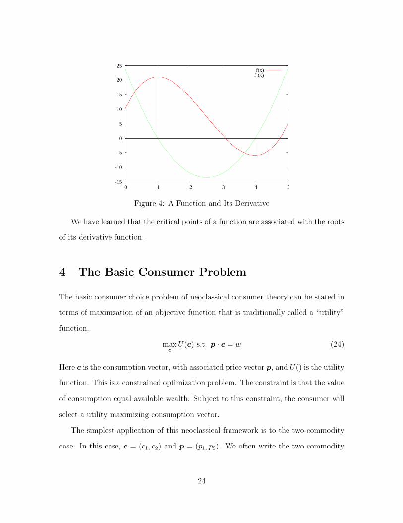
-15

-10

-5

0

5

10

15

20

25

0 1 2 3 4 5

f(x)f’(x)

Figure 4: A Function and Its Derivative

We have learned that the critical points of a function are associated with the roots

of its derivative function.

4 The Basic Consumer Problem

The basic consumer choice problem of neoclassical consumer theory can be stated in

terms of maximzation of an objective function that is traditionally called a “utility”

function.

maxcU(c) s.t. p · c = w (24)

Here c is the consumption vector, with associated price vector p, and U() is the utility

function. This is a constrained optimization problem. The constraint is that the value

of consumption equal available wealth. Subject to this constraint, the consumer will

select a utility maximizing consumption vector.

The simplest application of this neoclassical framework is to the two-commodity

case. In this case, c = (c1, c2) and p = (p1, p2). We often write the two-commodity

24

problem out more explicitly:

maxc1,c2

U(c1, c2) s.t. p1c1 + p2c2 = w (25)

Our first approach to this constrained optimization problem will be to transform

it into an unconstrained optimization problem. Let s be the amount spent on the

second commodity. Then c2 = s/p2 and the budget constraint implies c1 = (w−s)/p1.

So an equivalent formulation of the problem is

maxs

U

(w − sp1

,s

p2

)(26)

Note that we have taken a constrained optimization problem in two variables and

transformed it into an unconstrained optimization problem in one variable. (We will

explore other approaches later.)

The first order necessary condition for a maximum is4

∂U

∂c1

−1

p1+∂U

∂c2

1

p2= 0 (27)

This says that, at a maximum, each good’s marginal utility “per dollar” is the same.

That is, the additional utility of the last dollar spent on either good is equal. (Oth-

erwise the consumer would be able to raise utility by spending a dollar less on the

less rewarding good and a dollar more on the more rewarding good.) We sometimes

emphasize this description by restating this first-order condition as

MU1

p1=MU2

p2(28)

4In this section, we assume that utility is strictly concave, so our first-order necessary conditionwill also be sufficient for global maximum.

25

u(s;w,R)

ss*

Figure 5: Consumer Optimization: Plot of u(s)

Exercise 6

Given the utility function U(c1, c2) = c1/21 + c

1/22 , prices p = (1, 3)>, and wealth

of $10,000, what is your optimum consumption bundle? Set up and solve as an

unconstrained optimization problem.

Computational Exercise 2

Solve for the optimum level of saving in exercise 6 using Newton’s method. Use your

newton function from excercise 1. Note that you will be searching for the zeros of

the objective function’s derivative. (At the zeros of this derivative function we satisfy

the first-order condition.) To use Newton’s method for this search, we will therefore

need to provide information from the second derivative of our objective function. So

create the two functions you need, pick a sensible starting point for your algorithm

(say, 5000), and solve for optimal saving.

Optional supplement: graph the utility function on the subdomain (0, 10000] and

26

relate your graph to your numerical results.

27