ORF 307: Lecture 16

Linear Programming: Chapter 23:Integer Programming

Robert J. Vanderbei

April 16, 2019

Slides last edited on April 17, 2019

https://vanderbei.princeton.edu

Airline Equipment Scheduling

Given:

• A set of flight legs (e.g. Newark to Chicago departing 7:45am).

• A set of aircraft.

Problem: which specific aircraft should fly which flight legs?

Model:

• Generate a set of feasible routes (i.e., a collection of legs which taken together can beflown by one airplane).

• Assign a cost to each route (e.g. 1).

• Pick a minimum cost collection of routes that exactly covers all of the legs.

1

Let:

xj =

{1 if route j is selected,0 otherwise

aij =

{1 if leg i is part of route j,0 otherwise

cj = cost of using route j.

An Integer Programming Problem:

minimizen∑

j=1

cjxj

subject ton∑

j=1

aijxj = 1 i = 1, 2, . . . ,m,

xj ∈ {0, 1} j = 1, 2, . . . , n.

An example of set-partitioning problems.

2

Airline Crew Scheduling

Similar to equipment scheduling except:

It’s possible to put more than one crew on a flight:

• only one crew works• any others are just being shuttled

Integer Programming Problem:

minimizen∑

j=1

cjxj

subject ton∑

j=1

aijxj ≥ 1 i = 1, 2, . . . ,m,

xj ∈ {0, 1} j = 1, 2, . . . , n.

An example of set-covering problems.

3

Column Generation

The problem of producing a set of possible routes is called column generation.

It is important and nontrivial.

Reason: there are lots of routes.

For example, on a weekly schedule a route might consist of 20 legs.

If there are m legs in total, then there are up to m20 possible routes.

4

Traveling Salesman Problem

Most famous example of a hard problem:

Given n cities, determine the order in which to visit them so as to minimize the totaltravel distance.

5

Fixed Costs

A jump at x = 0:

c(x) =

{0 if x = 0K + cx if x > 0.

where0 ≤ x ≤ u.

Equivalent to:c(x, y) = Ky + cx

together with the following constraints:

x ≤ uy

x ≥ 0

y ∈ {0, 1}.

6

Nonlinear Objective Functions

Nonlinear objective functions are sometimes approximated by piecewise linear func-tions.

Piecewise linear functions can be treated using techniques similar to the fixed costmethod above.

LP Relaxation

General Integer Programming Problem

maximize cTxsubject to Ax≤ b

x≥ 0x has integer components.

7

Nonlinear Objective Functions

Nonlinear objective functions are sometimes approximated by piecewise linear func-tions.

Piecewise linear functions can be treated using techniques similar to the fixed costmethod above.

LP Relaxation

General Integer Programming Problem

maximize cTxsubject to Ax≤ b

x≥ 0//x ////has/////////integer///////////////components.

8

Example

9

Example with Upper/Lower Bounds

For the Branch and Bound method, we have introduced upper and lower bound constraints:

0 ≤ x1 ≤ 10, 0 ≤ x2 ≤ 10.

The number 10 is just taken to be some “very large” number (aka infinity). It will getchanged to smaller values as we go. 10

Optimal Solution to LP Relaxation

Optimal solution is (x1, x2) = (181/50, 21/10) = (3.62, 2.1) withobjective value 2813/50 = 56.26.

Rounding to integers: (4, 2) ⇐= infeasible.

Closest feasible: (3, 2) ⇐= suboptimal (as we’ll see). 11

First Branch of Branch&Bound Problem

Introduce an upper bound of 3 on x1:

Could solve this problem from scratch, or better yet...12

Start From Previous Optimal Dictionary

Originally, we had

t1 = 10− x1 = 10− 181/50 + 9/100w1 + 1/50w2

= 319/50 + 9/100w1 + 1/50w2

We change this too...

t1 = 3− x1 = 3− 181/50 + 9/100w1 + 1/50w2

= − 31/50 + 9/100w1 + 1/50w2

To summarize: upper bound decreases by 7, then the right-hand side for the upper bound’sslack variable decreases by 7. Everything else remains the same...

13

Start From Previous Optimal Dictionary

14

First Branch of Branch&Bound–Optimal Solution

Can be solved with just one dual pivot.

Here’s the optimal solution...

x1 is an integer but x2 is not. Gotta keep going. 15

Second Branch

Before working on x2, let’s ask what happens if we introduce a lower bound of 4 on x1.

Again, we start from the optimal solution to the original LP relaxation and just update oneright-hand side...

16

First Branch of Branch&Bound–Optimal Solution

INFEASIBLE!

17

Going Further Down the First Branch

Let’s go back to the scenario where x1 ≤ 3 and add an upper bound constraint of 2 on x2...

18

Our First All Integer Solution

It’s integers, but is it optimal?

Maybe not. Maybe we were wrong to impose the constraint x2 ≤ 2.

Maybe it’s better to give x2 a lower bound of 3. Let’s see...

19

A Second Branch Below the First Branch

20

Another All Integer Solution

And, look at the objective function value.

This one’s better than the one we had before.

There’s no more branching to do. We are done. This is the OPTIMAL SOLUTION!!

21

Gomory Cuts Method

Here’s the same problem again:

NOTE: Seed value 6 in Gomory pivot tool.

22

LP Relaxation

Here’s the solution to the LP relaxation:

Neither x1 nor x2 are integers!

23

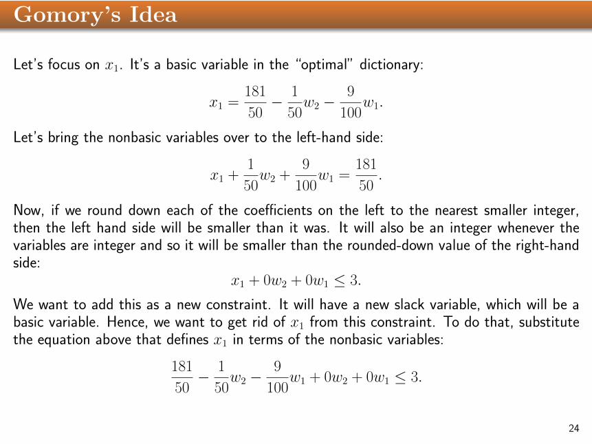
Gomory’s Idea

Let’s focus on x1. It’s a basic variable in the “optimal” dictionary:

x1 =181

50− 1

50w2 −

9

100w1.

Let’s bring the nonbasic variables over to the left-hand side:

x1 +1

50w2 +

9

100w1 =

181

50.

Now, if we round down each of the coefficients on the left to the nearest smaller integer,then the left hand side will be smaller than it was. It will also be an integer whenever thevariables are integer and so it will be smaller than the rounded-down value of the right-handside:

x1 + 0w2 + 0w1 ≤ 3.

We want to add this as a new constraint. It will have a new slack variable, which will be abasic variable. Hence, we want to get rid of x1 from this constraint. To do that, substitutethe equation above that defines x1 in terms of the nonbasic variables:

181

50− 1

50w2 −

9

100w1 + 0w2 + 0w1 ≤ 3.

24

25

Now we just do a dual pivot to get to a new “optimal” solution:

We still have a non-integer value: x2 = 22/9.

26

Let’s make another Gomory cut:

x2 +1

9w2 −

5

9w2+1 =

22

9.

Rounding down...x2 + 0w2 − w2+1 ≤ 2

New constraint...22

9− 1

9w2 +

5

9w2+1 + 0w2 − w2+1 ≤ 2

27

Again, we do a dual pivot:

OPTIMAL!

28