Oregon Department of Education Summary of Score ...
46
Oregon Department of Education Summary of Score Comparability Analyses Grade 3 Spanish Reading Pilot, 2009-10 Office of Assessment and Information Services, Oregon Department of Education 6/28/2010 Document 3
Transcript of Oregon Department of Education Summary of Score ...
Oregon Department of Education
Summary of Score Comparability Analyses Grade 3 Spanish Reading Pilot, 2009-10
Office of Assessment and Information Services, Oregon Department of Education 6/28/2010
Document 3
2
Summary of Score Comparability Analyses
Introduction
Tests translated into a second language present various challenges to providers attempting to construct
comparable measures of performance and to users attempting to make comparable inferences with the
scores. One goal in designing a comparable measure is to standardize in ways that control for errors.
Language differences present a natural barrier to standardization that is challenging to overcome. Words
may have various contextual and cultural meanings that do not fully translate across languages in a concise
manner. Validity demands that inferences made with the scores are comparable across forms of the test
and that the classificatory decisions made with the scores are accurate.
A valid reading test in English that has a parallel or homologous equivalent in Spanish would provide a
valuable approach when making comparable decisions regarding the learning of second language
populations. To be successful, the items would need to be comparable in content and task, functioning
equivalently for students at a given ability level. Such a test would permit policy makers the opportunity to
observe changes in the reading scores of Spanish speaking populations and relate those findings to the
changing scores of the more common English speaking counterparts. For any set of tests designed for cross
language comparisons, inferences or claims made with the test scores can only be interpreted when the
same construct is measured on a comparable scale or metric. Despite our intentions, different socio-
cultural factors and academic variables like class differences, gender, translation, and curriculum
differences potentially confound our attempts to produce comparable measures. As a result, one analyzes
the degree of comparability achieved by the English and Spanish Reading scales and items, demonstrating
how potential differences affect the policy decisions made with the scores.
Background of the Study
One important source of construct-irrelevant variance is the language used to assess the examinees.
Language factors as potential threats to the construct validity of the test has been addressed within the in
the 1999 Standards of Educational and Psychological Testing. Score interpretation is an important aspect of
any state test. Previous research has shown that tests administered in different languages may not provide
comparable scores (Hambleton, 1994; Gierl & Khaliq, 2001). Although Oregon primarily reports data for
schools and districts in terms of “meeting “or “not meeting” a performance standard, scale scores are
reported to parents and become part of the school record.
Structure Equations modeling has also been used to examine test structure and the scaling metric across
multiple groups (see Gierl & Khalig, 2001; Serici & Khaliq, 2002; Wu, Li, and Zumbo, 2006), using an a priori
specification of hypotheses testing of increasingly more restrictive models. Serici and Khaliq (2002) found
that the factor loadings and error variances were not equivalent across language groups. These slight
differences were mainly attributed to overall group proficiency differences.

3
Differential item functioning (DIF) has been previously used to examine the probability of comparable
groups taking the test in different language getting the transadaptive items correct. In fact, although
students are taking tests in their native language, there are many examples of studies that demonstrated
differential functioning in translated items was pervasive (over 30% of the items) and potentially affected
student performance (e.g., Gierl & Khaliq, 2001; Ercikan & Koh, 2005; and Sireci & Khaliq, 2002). Items
flagged for DIF often had inconsistent terms or the language used was less familiar.
Because Oregon reading scores in grade 3 are reported against a performance standard, the common
practice is to make meeting/not meeting distinctions with the state’s school and district results. Guo (2006)
proposed a method for assessing the accuracy for tests used to classify students into different
classifications. This latent distribution method will be used to compare scores obtained using Spanish item
calibrations and scores obtained using English item calibrations. In addition, the means and standard
deviations for both scores will also be compared.
Although not directly studied, there may be advantages in using adaptive tests over paper tests when
attempting to achieve comparability in language tests. The expected value and derived variances of an
adaptively generated set of random forms administered to a large sample from a large item pool might
provide some improvement over the fixed forms typically used with paper-and-pencil tests.
With these thoughts in mind, the first purpose of this study is to examine scale and item comparability
using the state reading tests offered in both English and Spanish languages. A second but related purpose
is to evaluate the classification accuracy of the scores to determine their usefulness in decision making visa
via the standard. Given sufficient items and students, one attempts to analyze the veracity of the claim that
the measures are comparable for their intended purpose.
Translation and Adaption Efforts
The No Child Left Behind (NCLB) Act requires states that have assessment systems that include both a
regular assessment in English and a non-English version of that assessment to demonstrate that these two
assessments are comparable and aligned with the same academic content standards. The application of a
set of items to a new culture is more complex than merely translating the items (Hambleton, 1994; Van de
Vijuer & Hambleton, 1996). There are many factors that jeopardize the validity of intergroup comparisons.
Anomalies in specific items and test administrations as well as the challenge of generalizing theoretical
constructs across two or more cultures limit our ability to achieve measurement comparability (Van de
Vijuer & Hambleton, 1996).
A methodical set of procedures must be employed during item development to ensure the accuracy of the
transadaptions and to ensure that the same knowledge, skills, and abilities are being assessed in both
languages. Periodic reviews are undertaken to ensure that the items are being translated or adapted
properly and that the same knowledge, skills, and ability are being tested. Data obtained from this study
will be used to improve item development practices and the test’s construct validity.

4
Sampling and Methodological Considerations
A sample of 855 tests was randomly selected from students taking the OAKS grade 3 English Reading tests
and compared with the 855 grade 3 Spanish Reading tests administered in April 2010. Since the Spanish
Reading group is self selected, it is difficult to evaluate their comparability in an even handed fashion. For
this reason, successive tests of equivalence are applied to evaluate varying degrees of scale comparability.
DIF applies matched sampling in an effort to produce comparable groups across several ability levels. To
obtain comparable groups for DIF analysis of a given item, a sampling program first matches the
distribution of the scores of students in the referent group to the existing distribution of scores of students
in the focal group who received the same item. The program then segments the focal group’s score
distribution into ten intervals, and then randomly selects students from the reference group with scores
that match the focal group within each interval. So, for example, if 5% of the students in the focal group
had scored between 200 and 210 on the test, the sampling program would match the scores of students in
referent group until 5% of those scores were between 200 and 210. This matching procedure is performed
across the entire distribution of scores in the focal group until a similar distribution of matched scores was
generated for the reference group. If sufficient numbers of students were available at each ability level, the
item means and standard deviations were approximately equal for both the focal and reference groups
after sampling.
Analyses
Steps in Examining the Empirical Comparability of the Measures are summarized below. These methods
have been previously employed in such research (see Sereci & Khaliq, 2002).
1. Different conceptions of comparability can be attained for a given set of scales. The first step is to
check whether the observed measures possess congeneric equivalence, essentially tau equivalence,
and parallel equivalence using confirmatory factor analysis (CFA). The CFA framework tests these
measurement comparability properties by comparing hierarchical models using the chi-square
difference test.
2. Item comparability promotes conditions where the probability of achieving a correct response is
equal given chance levels of difference. A second step checks for item comparability by the two
populations using DIF methods that controls for differences in group performance. Tests of the
odds ratio or some form of a logistic regression model are considered more appropriate at the item
level. Mantel Haenszel and logistic regression are employed item by item to check for uniform and
non-uniform differences in item functioning.
3. Scores are ultimately employed against a performance standard as a means of judging successful
performance. A latent distribution method is employed as a final step to calculate the expected
5
classification accuracy of the Spanish and English test in classifying students at the cut score.
Scores that yield comparable results given these pass/fail determinations produce higher observed
rates that closely matches the expected or modeled classification accuracy.
Scale Level Analysis
Varying conceptions of parallel equivalence provide one means of evaluating test comparability (see Feldt
and Brennan, 1989; Graham, 2006). Parallel equivalence assumes the most restrictive model requiring that
any examinee belonging to a given language group has the same true score no matter what form of the test
is produced by either the Spanish or English pool. Administered forms are comprised of comparable items
that are translated into Spanish or English, content balanced to a test blue print, and tailored to an ability
estimate. Parallel equivalence demands equal mean scores, observed variances, and error variances on
every form in order to produce equal true scores. Scales that have parallel equivalence produce
interchangeable item calibrations and student scores, but parallel equivalence is difficult to attain when
testing in different languages.
Relaxing one or two restrictions employed by the parallel model allows for an alternative conception of
comparability. Because the Spanish reading group is self selected and the number of students testing in
Spanish is much smaller than in English reading, it is difficult to evaluate parallel equivalence in an even
handed fashion. For this reason, tests of tau or essential tau equivalence are alternatively proposed and
applied as a possible accommodation to this inherent challenge. Tau equivalence permits the error
variances to vary where the purely parallel model does not. The relaxation of error assumption still allows
for a common scale with equal item locations with comparable precision, but each subscale has unique
error variance. By further relaxing restrictions, essential tau equivalence differs from tau equivalence in
that it permits scales to differ by a constant (Feldt & Brennan, 1989; Graham, 2006). Despite this
difference in item location and scale precision, essential tau equivalence still produces comparable
measures that still share a common scale but have mean and unique error differences associated with each
subscale or strand reporting category (SRC). Because the reliability coefficient is typically calculated as a
ratio of true and observed variance, essential tau equivalent models produce reliability coefficients that are
comparable to tau equivalent scales. However, as long as differences in the scale location terms exist
between language groups, imprecision will always exist in some form on each scale and these constant
differences will likely favor lower performers (Bollen, 1989). Differences between essential tau equivalence
and tau equivalence are discussed in more detail by Feldt & Brennan (1989) and Graham (2006).
Congeneric equivalence provides the least restrictive test of comparability. The means, observed
variances, and error variances of the scale scores are permitted to vary, but the true scores are still
perfectly correlated. This result suggests that the produced factor structure is measuring the same latent
construct.

6
The Measurement Model
As specified by the two-group model below, local independence of each subtest holds when the latent
variable, , accounts for the variance in the unidimensional model and the errors, i, are unique and
statistically independent.
iy1 =
i1 + i1
+ i1
…
jy2=
j2 + j2 + j2
Where iy1 is an observed measure regressed on the first sample’s latent variable to estimate a
factor coefficient, i1 , and intercept, i1 , while j is the number of factors in the model. This
factor model maintains that when two or more groups share the same regression line, then the
scale is operating the same way for any sample.
Congeneric measures possess a common factor structure but do not share the same levels of
precision as other forms of measurement. When the population variance/covariance matrix is
equal for both groups and across both forms of the test, the factor structure of the two forms of
the test is similar.
Essentially tau equivalent measures assume that the slopes measuring the changes in the observed
variables ( iy1 .. jy2 ) given a unit change in the latent variable ( )are invariant across the two tests
(i.e, i1 =…. j2 ), but these true values may lack precision when their modeled intercepts differ
(Graham, 2006). Factor loadings that are essentially tau equivalent share a common slope, so they
contribute in comparable ways to the true scores and the calibrated values are said to share a
common latent scale. Factor loadings that do not share common slopes contribute variance that is
unique to the observed variables (y ij ) and this effect increases measurement error. In other words,
congeneric factors that lack essential tau equivalence share the same trait but are less likely to
share the same scale.
A factor analytic model with equal error variance constrained across subscales and groups
( i1 =…. j2 ) provides more consistent and stable measurement across groups and forms of the
test. For this reason, these measures are said to be parallel in form. Applying a classical
perspective, the ratio of item true score variances to the sum of the item true scores variances and
error score variances are similar for forms of the test and the two populations taking the items.
When error variances are heterogeneous, the observed variables measure the latent trait with
different amounts of error and are less comparable.

7
Item Level Analysis
Differential Item functioning describes a set of analytical practices for determining whether any item
operates fairly for different groups (see Holland and Wainer, 1993). DIF is defined as an item that displays
different statistical properties for different manifest groups after controlling for levels of ability (Angoff,
1993). The presence of DIF implies that the item measures more than one latent trait. Large DIF effects
are necessary conditions when evaluating potential item bias, but group differences in item functioning do
not always imply that the item is biased. There are true differences between groups that one wishes to
validly and reliably measure, but DIF attempts to measure only nuisance factors that confound the
measurement of the true scores, thereby creating construct irrelevant differences that were largely
unintended (Camilli, 2006). Competing explanations can often occur that better explain these differences,
especially when similar patterns exist across various items within a specific content area. Judgmental or
logical analysis must then be used to make an ethical decision regarding the future use of the item.
Typically, the item performance of two groups is compared: the referent group and the focal group.
Students taking the English Reading test are hereby known as the referent group; students taking the
Spanish Reading test are herby know as the focal group. In this study, to ensure comparability, English
passages and reading test items are independently translated to Spanish by two translators. Students taking
a reading test in Spanish are assigned to the focal group, while students taking a reading test in English are
assigned to the referent group. To be considered comparable, the item performance of the Spanish
speaking students at a given level of ability should be equal to the item performance of English speaking
students at an identical level of ability on comparable items.
There are two forms of DIF that potentially occur: uniform DIF and non-uniform DIF (see Zumbo, 1999).
With uniform DIF, the differences in item functioning always favor the same group no matter what the
ability level. Item characteristic curves (ICC) in Figure 1 are parallel so they differ in a uniform manner, with
the referent group having a higher probability of getting the item correct at each ability level. With non-
uniform DIF, the differences in item functioning can differ depending on the ability level of the groups. Non-
uniform DIF is illustrated in Figure 2 where the amount of DIF varies by levels of the RIT scale. The group
favored by the item is determined by the level of ability – the focal group is favored at the top of the scale
while the referent group is favored at the bottom of the scale.

8
Figure 1
Figure 2
9
Mantel-Haenszel Procedure: Holland (1985) proposed the use of the Mantel-Haneszel procedure as a
practical and powerful way to detect test items that function differently for two matched groups of
examinees. A 2x2 cross-tabulation table is produced for the previously matched set of examinees in both
the reference and focal groups over each of the K levels of ability. The Mantel-Haenszel procedure tests
the null hypothesis that the common odds ratio of correct response across all matched groups is = 1
over the K levels. Mantel and Haenszel developed an estimator of whose scale ranges from 0 to
known as alpha (̂ ), so an obtained value of ̂ =1 implies that there is negligible or no DIF. A small,
obtained value less than 1 favors the focal group, while a large value greater than 1 favors the referent
group.
Logistic Regression: The Mantel-Haenszel method assumes that only the difficulty of the items may change,
and item DIF is detected by simultaneously testing for significant group differences in the odds ratio at K
ability levels. Like the Mantel-Haenszel procedure, the logistic regression first tests for “uniform”
differences in the responses represented by comparing the fit of the model. This is done by first fitting a
model relating the dichotomous response of the item to the scale score and calculating a chi-square value.
A second model expands on the first model by adding a group variable to the original model and using the
likelihood ratio test (1 df) to examine changes in the fitted model. By subtracting the chi-square value of the
second model from the first, a likelihood chi-square test of difference is calculated. A significant change in
model fit means there is significant uniform DIF. This approach has been shown to be mathematically
comparable to the Mantel Haenszel result. Shultz and Geisinger (1992) found that the agreement between
the logistic regression and the Mantel Haenszel procedure declines with decreased sample size or when the
number of levels employed by the Mantel Haenszel is less than 10. Zumbo (1999) suggested minimum
samples of size 200 or larger to evaluate items with DIF with logistic regression.
Examining the effect size in the difference in difficulties is as important as the test of significance in both
the Mantel Haenszel and logistic regression when identifying items with DIF. This strategy is typically
adopted because one wants to control for statistical inflation in Type I and Type II error rates attributed to
the number of tests and sample size when using the Likelihood Chi-square test over a number of items.
Zieky (1993) and Jodin and Gierl (2001), respectively, developed DIF classification systems for the Mantel-
Haenszel and logistic regression taking both the test of significance and effect size into account. For Mantel
Haenszel, Zieky used the absolute value of the magnitude in change in delta () to determine moderate or
large effect sizes. Delta () is equal to -2.35 ln(), where is the common odds ratio. When the absolute
value of the delta difference is at least 1 and less than 1.5, the effect is moderate in size. When the
absolute value of the delta difference is at least 1.5 or great, the effect is large in size. For logistic
regression, Jodin and Gierl (2001) recommend using a 0.035 Nagelkerke R 2 0.07 for moderate DIF
and 0.07 Nagelkerke R 2 for large DIF. Nagelkerke R 2 is a “pseudo” r-squared value associated with the
logistic regression and, like the R 2 used in any linear regression, ranges between 0 and 1.
Unlike the more restrictive Mantel Haenszel method, logistic regression goes further by testing whether the
item discriminates equally well across the ability distribution. Items with non-uniform DIF identify groups
10
who have advantage over a second group in one area of the distribution, but are at a disadvantage at
another end of the distribution. One way to test for such differences in the rates of growth between
groups is to fit a model that adds an interaction term to the second model. This third model with its RIT
term, its group term, and its RIT by group interaction term is fitted and a change in the chi-square value is
calculated by subtracting the chi-square value of the third model from the second model. Any significant
change in chi-square would suggest non-uniform DIF.
Model 1 z = β0
+β 1 X
Where P=probability of a correct response, z = ln(P/Q), and Q=1-P
A second model expands on the first model by adding a group variable to the original model and using the
likelihood ratio test (1 df) to examine changes in the fitted model.
Model 2 z = β 0 +β 1 X +β 2 G
A third model with its RIT term, its group term, and its RIT by group interaction term is fitted and a change
in the chi-square value is calculated by subtracting the chi-square value of the third model from the second
model.
Model 3 z = β0
+β 1 X +β 2 G + β3
XG
A likelihood ratio difference test between the models is then employed to determine successive values of
G. Comparing Chi-square distributions with the appropriate degrees of freedom yields a p-value that
explains how much the new variable adds to the model.
G = χ 2 = D(compact model) – D(augmented model)
=D 1model - D 2model
=D 2model - D 3model
Decision Level Analysis
A third important consideration when evaluating score comparability involves the usefulness of the score
for making classification decisions. Every time one makes a decision with a standard there is bound to be
some number of misclassifications (Rudner, 2001).
11
An accuracy or classification index estimates the number of examinees that are correctly classified. The
higher the index of accuracy, the more likely a student will be classified given his/her score. A classification
index compares an observed and expected classification rate using item response theory approach.
A latent distribution method developed by Guo (2006) is employed to examine the classification accuracy in
the two tests. The latent distribution method has at least two advantages over a method developed by
Rudner (2001): 1.) Guo ‘s method makes fewer assumptions and is easier to calculate and 2) the analysis is
less problematic to perform on ability estimates derived when smaller numbers of items are administered.
The Spanish and English reading results of the latent distribution method are than compared using the
scores on the Spanish tests calculated from the Spanish pool and the sample student scores calculated from
the English pools.
Results
Confirmatory Factor Analysis of the Results
Preliminary analysis independently fits a one factor model to the both the Spanish Reading data and the
English Reading data with the results presented in Table 1. Previous Exploratory Factor Analysis (EFA)
revealed one strong latent effect for both the Spanish and English Reading tests explained by the four
observed variables: vocabulary, reads to perform, demonstrates understanding, and develops
interpretations. All residuals calculated when subtracting the sample and reproduced variance/covariance
matrix were near 0. One eigenvalue explained over 75 percent of the variance in both tests, and this first
factor produced the only eigenvalue greater than 1. The scree plot strongly suggested the existence of one
factor being explained in both analyses.
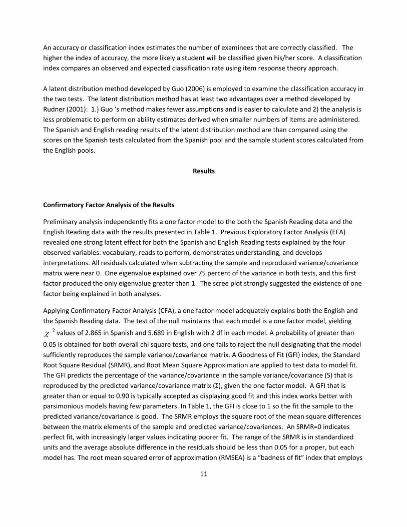
Applying Confirmatory Factor Analysis (CFA), a one factor model adequately explains both the English and
the Spanish Reading data. The test of the null maintains that each model is a one factor model, yielding
2 values of 2.865 in Spanish and 5.689 in English with 2 df in each model. A probability of greater than
0.05 is obtained for both overall chi square tests, and one fails to reject the null designating that the model
sufficiently reproduces the sample variance/covariance matrix. A Goodness of Fit (GFI) index, the Standard
Root Square Residual (SRMR), and Root Mean Square Approximation are applied to test data to model fit.
The GFI predicts the percentage of the variance/covariance in the sample variance/covariance (S) that is
reproduced by the predicted variance/covariance matrix (Σ), given the one factor model. A GFI that is
greater than or equal to 0.90 is typically accepted as displaying good fit and this index works better with
parsimonious models having few parameters. In Table 1, the GFI is close to 1 so the fit the sample to the
predicted variance/covariance is good. The SRMR employs the square root of the mean square differences
between the matrix elements of the sample and predicted variance/covariances. An SRMR=0 indicates
perfect fit, with increasingly larger values indicating poorer fit. The range of the SRMR is in standardized
units and the average absolute difference in the residuals should be less than 0.05 for a proper, but each
model has. The root mean squared error of approximation (RMSEA) is a “badness of fit” index that employs
12
a non-central chi square distribution and produces a confidence interval. A RMSEA less than 0.05 indicates
a lack of “bad” fit, and both models meet this standard. A confidence band of 90% is presented and there is
a greater potential for misfit at the higher end of the scale.
Single Group Analysis Model Fit
Table 1
Model Fit 2 df P-Value RMSEA GFI SRMR
Spanish Reading 2.865 2 .239 0.023 (0, 0.075) 998 0.0081
English Reading 5.689 2 .058 0.046 (0, 0.093) .997 0.0039
N=855 per group tested
Hierarchical Test Statistics and Fit Indices
Using CFA, one evaluates measurement equivalence using a hierarchical procedure that compares a
number of increasingly more restrictive models using a likelihood ratio goodness of fit difference test along
with a comparative fit index. Since most models are either slightly misspecified or do not account for all
measurement error, when sample sizes are large, a nonsignificant chi-square test is rarely obtained.
Because a researcher’s model is so frequently rejected in large samples, other measures of fit have been
developed to assess the congruence of model fit to the data. A better fitting model does not always mean
a more correct model.
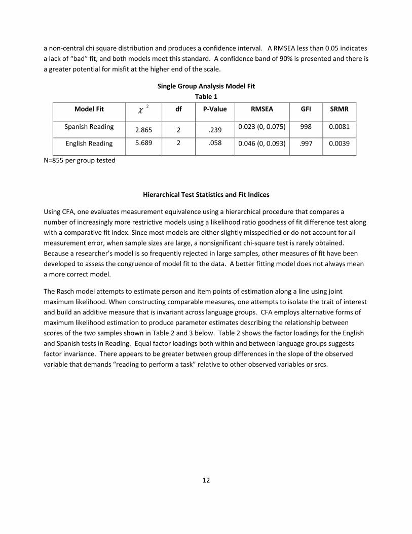
The Rasch model attempts to estimate person and item points of estimation along a line using joint
maximum likelihood. When constructing comparable measures, one attempts to isolate the trait of interest
and build an additive measure that is invariant across language groups. CFA employs alternative forms of
maximum likelihood estimation to produce parameter estimates describing the relationship between
scores of the two samples shown in Table 2 and 3 below. Table 2 shows the factor loadings for the English
and Spanish tests in Reading. Equal factor loadings both within and between language groups suggests
factor invariance. There appears to be greater between group differences in the slope of the observed
variable that demands “reading to perform a task” relative to other observed variables or srcs.
13
Maximum Likelihood Estimates of the Two Samples Table 2
Reading in English Factor Slopes Standard Error of Slope Vocabulary 1.00 (fixed) --
Read to perform a task 0.969 .040 Demonstrate understanding 1.025 .036 Develop and interpret 0.935 .034
Reading in Spanish Factor Slopes Standard Error of Slope Vocabulary 1.00 (fixed) --
Read to perform a task 1.228 .066 Demonstrate understanding 1.092 .051 Develop and interpret 1.031 .050
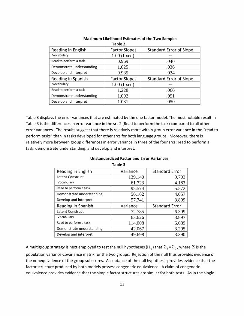
Table 3 displays the error variances that are estimated by the one factor model. The most notable result in
Table 3 is the differences in error variance in the src 2 (Read to perform the task) compared to all other
error variances. The results suggest that there is relatively more within-group error variance in the “read to
perform tasks” than in tasks developed for other srcs for both language groups. Moreover, there is
relatively more between group differences in error variance in three of the four srcs: read to perform a
task, demonstrate understanding, and develop and interpret.
Unstandardized Factor and Error Variances
Table 3
Reading in English Variance Standard Error Latent Construct 139.140 9.703 Vocabulary 61.723 4.183 Read to perform a task 95.574 5.572 Demonstrate understanding 56.162 4.057 Develop and interpret 57.741 3.809
Reading in Spanish Variance Standard Error Latent Construct 72.785 6.309 Vocabulary 63.626 3.897 Read to perform a task 114.008 6.689 Demonstrate understanding 42.067 3.295 Develop and interpret 49.698 3.390
A multigroup strategy is next employed to test the null hypotheses (H 0 ) that 1 = 2 , where is the
population variance-covariance matrix for the two groups. Rejection of the null thus provides evidence of
the nonequivalence of the group subscores. Acceptance of the null hypothesis provides evidence that the
factor structure produced by both models possess congeneric equivalence. A claim of congeneric
equivalence provides evidence that the simple factor structures are similar for both tests. As in the single

14
group analysis, a SRMR index is calculated to examine the absolute fit of the sample estimates to the
implied or predicted variance/covariance matrix at each stage of the hierarchical analysis.
Subsequent chi-square difference tests are next performed to test the increasingly more restrictive
assumptions associated with essential tau and parallel equivalence. Statistical Tests are applied by
constraining parameters in a restrictively increasing fashion and by observing changes in the chi-square
likelihood test ( 2 ). Each time one tests the differences in the likelihood chi-square statistics ( Δ 2 ) in
the augmented model minus the more compact model. A p-value is computed for each change in the chi-
square statistic. A good fitting comparative model will have a Δ 2 p-value greater than 0.05,
demonstrating that the differences in the likelihood square statistic are negligible.
Two subsequent fit indices are applied: the Root Mean Square Error of Approximation (RMSEA) and the
Comparative Fit Index (CFI). RMSEA takes into account errors in approximation by asking, “How well would
a model, with unknown but optimally chosen parameters values, fit the population variance/covariance
matrix if it were available? “(see Browne and Cudek, 1993). A noncentrality parameter is estimated from a
an approximate noncentral chi-square distribution, designated as . The value of increases as the null
becomes more false. Using Cheung and Resvold’s (2002) recommendations, reasonable errors in
approximation would be equal to or less than 0.05.
The CFI is a fit index that provides further utility when assessing the fit of two competing models. The CFI is
not sensitive to large sample sizes and is derived by a comparison of the hypothesized model to an
independence model. Again using Cheung and Resvold’s (2002) recommendations, the change in CFI (ΔCFI)
should be less than or equal to -0.01, which is a more robust test than the commonly used standard of
accepting model fit for any CFI greater than 0.95.
As already mentioned, each subsequent test is more restrictive since additional variance constraints are
being placed on the hypothesized model. For instances, considering the first test, congeneric indicators
measure the same construct but not to the same degree of accuracy. The CFA model for congenerity does
not impose any constraints or restrictions on the model. If this factor structures is different across groups,
the null hypothesis would be rejected due to a lack of model fit. However, as in the present case, if the
model fits the data reasonably well, the congeneric sets of indicators are said to possess convergent validity
so the four indicator variables measure the same latent variable, but the latent measures may be on
different scales. One can then proceed to the test of essential tau equivalence to determine otherwise.
A difference test of essential tau equivalence fixes all the factor loadings equal to 1 and evaluates whether
the model is both congeneric and whether the score reporting categories (src’ s)have equal factor loadings.
Internal measures of consistency like Cronbach’s Alpha assume essential tau equivalent measures (see
Raykov, 1997; Graham, 2006). If the fit of the model to the data violate the essential tau equivalent
assumption, it is possible that a strong simple structure factor analytic model will produce latent measures
on different scales with spuriously low reliability. Rejection of the null hypothesis of no differences implies
that the true scores significantly vary over the score reporting categories (src). However, in this case, the fit
indices present a different story when compared to the rejected equal factor loadings hypotheses of the
15
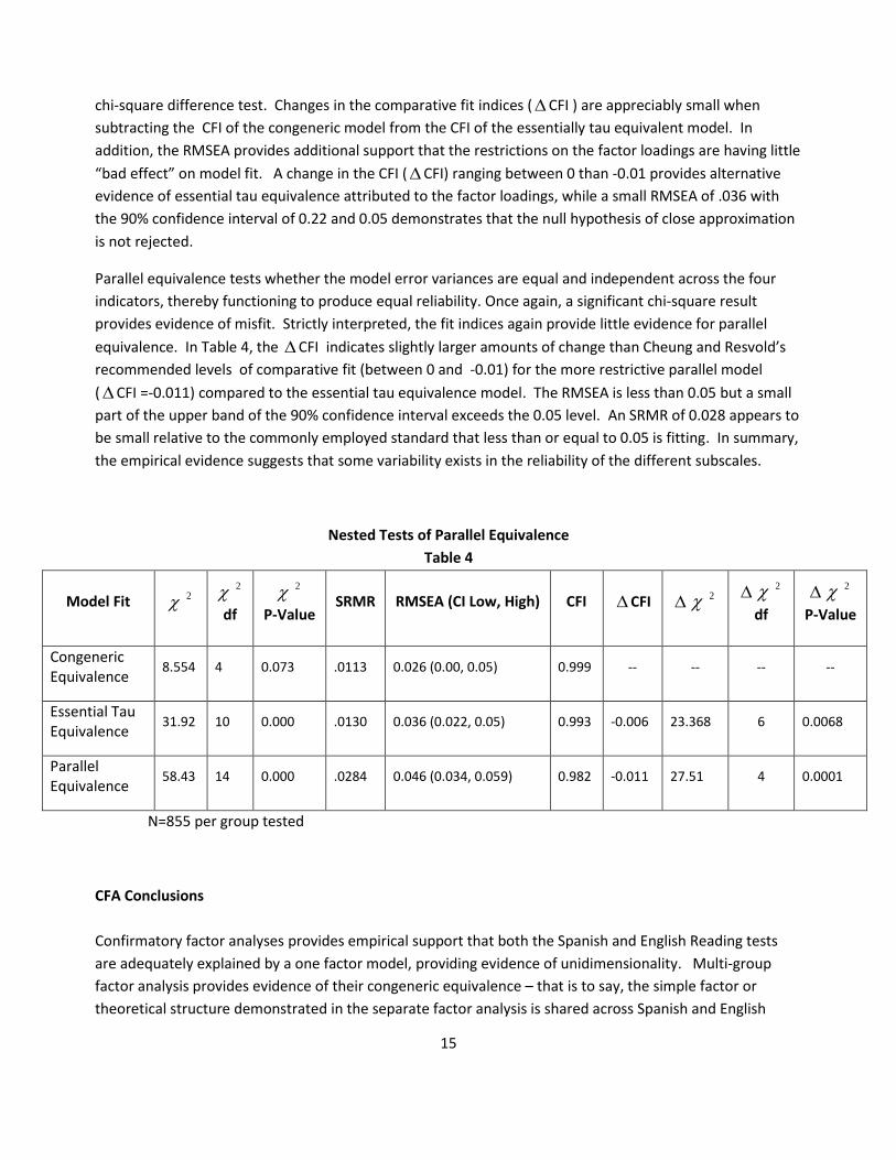
chi-square difference test. Changes in the comparative fit indices (CFI ) are appreciably small when
subtracting the CFI of the congeneric model from the CFI of the essentially tau equivalent model. In
addition, the RMSEA provides additional support that the restrictions on the factor loadings are having little
“bad effect” on model fit. A change in the CFI (CFI) ranging between 0 than -0.01 provides alternative
evidence of essential tau equivalence attributed to the factor loadings, while a small RMSEA of .036 with
the 90% confidence interval of 0.22 and 0.05 demonstrates that the null hypothesis of close approximation
is not rejected.
Parallel equivalence tests whether the model error variances are equal and independent across the four
indicators, thereby functioning to produce equal reliability. Once again, a significant chi-square result
provides evidence of misfit. Strictly interpreted, the fit indices again provide little evidence for parallel
equivalence. In Table 4, the CFI indicates slightly larger amounts of change than Cheung and Resvold’s
recommended levels of comparative fit (between 0 and -0.01) for the more restrictive parallel model
(CFI =-0.011) compared to the essential tau equivalence model. The RMSEA is less than 0.05 but a small
part of the upper band of the 90% confidence interval exceeds the 0.05 level. An SRMR of 0.028 appears to
be small relative to the commonly employed standard that less than or equal to 0.05 is fitting. In summary,
the empirical evidence suggests that some variability exists in the reliability of the different subscales.
Nested Tests of Parallel Equivalence
Table 4
Model Fit 2 2
df
2
P-Value SRMR RMSEA (CI Low, High) CFI CFI 2
2
df
2
P-Value
Congeneric Equivalence
8.554 4 0.073 .0113 0.026 (0.00, 0.05) 0.999 -- -- -- --
Essential Tau Equivalence
31.92 10 0.000 .0130 0.036 (0.022, 0.05) 0.993 -0.006 23.368 6 0.0068
Parallel Equivalence
58.43 14 0.000 .0284 0.046 (0.034, 0.059) 0.982 -0.011 27.51 4 0.0001
N=855 per group tested
CFA Conclusions
Confirmatory factor analyses provides empirical support that both the Spanish and English Reading tests
are adequately explained by a one factor model, providing evidence of unidimensionality. Multi-group
factor analysis provides evidence of their congeneric equivalence – that is to say, the simple factor or
theoretical structure demonstrated in the separate factor analysis is shared across Spanish and English
16
forms of the test. A simple factor or latent trait is an unobserved construct measured by the test – in this
case, reading achievement. In substantive research, it is important to know whether the factor loadings and
the relations among the strand reporting category scores are equivalent across forms of the test, because a
unit increase their latent score translates into a unit increase in each strand reporting category score. Chi-
square tests of equal slopes of the strand score factor loadings on the latent trait are significant, suggesting
some linear differences in growth trajectories of each test. Although this result suggests that strand
reporting scales are not strictly operating in the same way, any between language differences the strand
variable scales viewed in Table 3 appear to be due to sample variation. Comparative fit indices provide
evidence for the confirmation of the essential tau equivalence models, entailing a congeneric solution in
which the indicators of a single factor have equal factor loadings but different error variances. This
essential tau equivalence suggests that a unit change in each strand score translates into a unit change in
the latent score, but that any change is different by some constant. Because there was evidence of
essential tau equivalence, a more restrictive model was tested. This further tests of parallel equivalence
yielded additional mixed results given its more restrictive assumptions of equal error variances. Models
with equal error variances have equal reliability and produce interchangeable true scores across forms of
the test. Such a result would exhibit the highest standards of comparability and is seldom achieved in
practice.

17
DIF Results
Tests of item invariance provide a second method for assessing measurement equivalence. The odds of
success for students taking an English Reading item should be equal to those students taking a comparable
Spanish item when the underlying ability level is the same. Mantel-Haenszel DIF analysis is employed to
test this underlying assumption for each of the 169 comparable items written for both the Spanish and
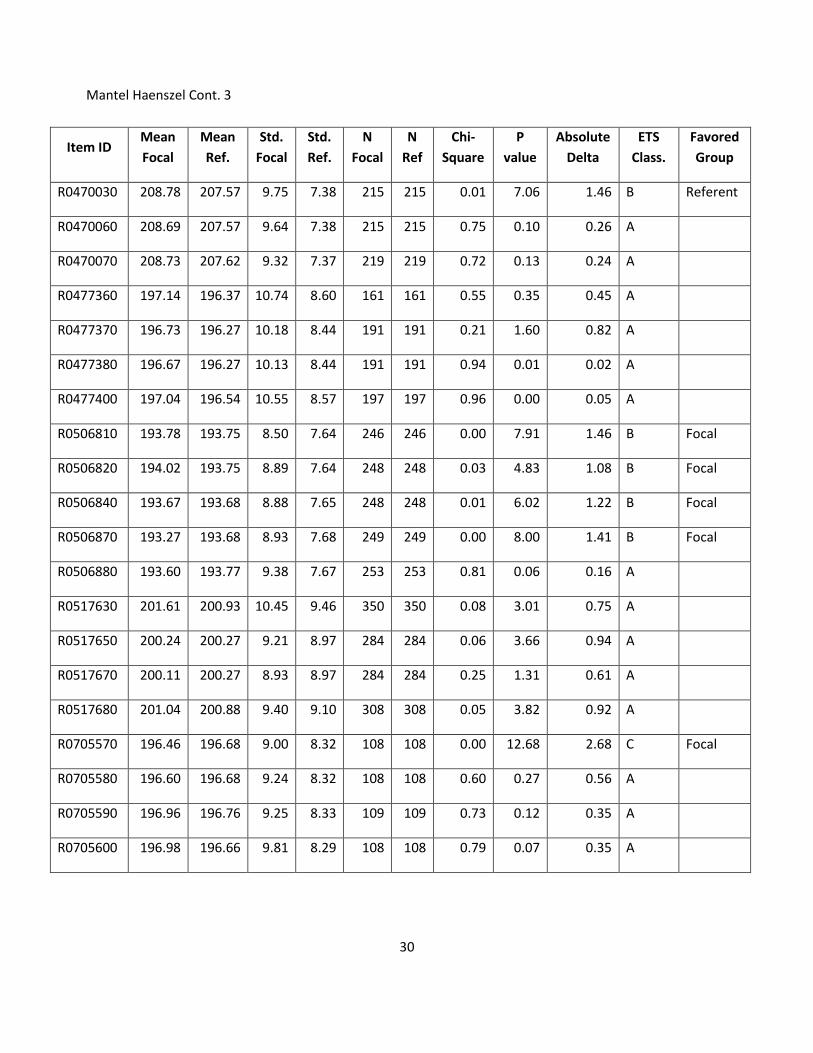
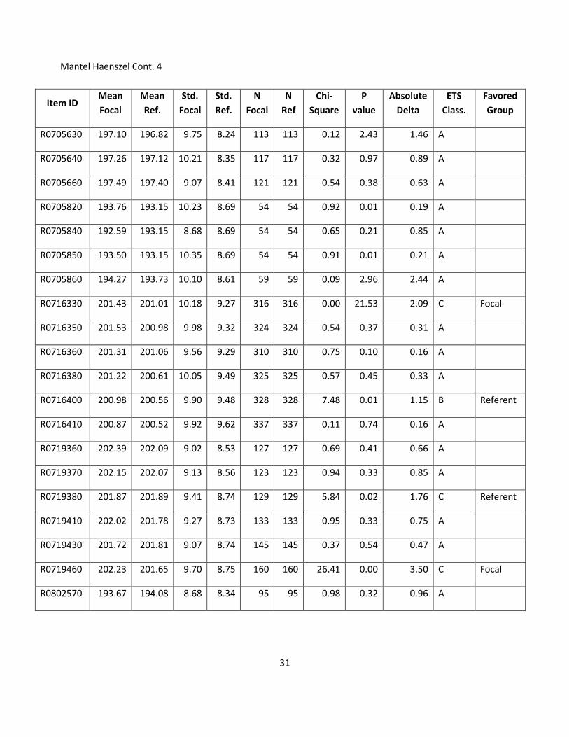
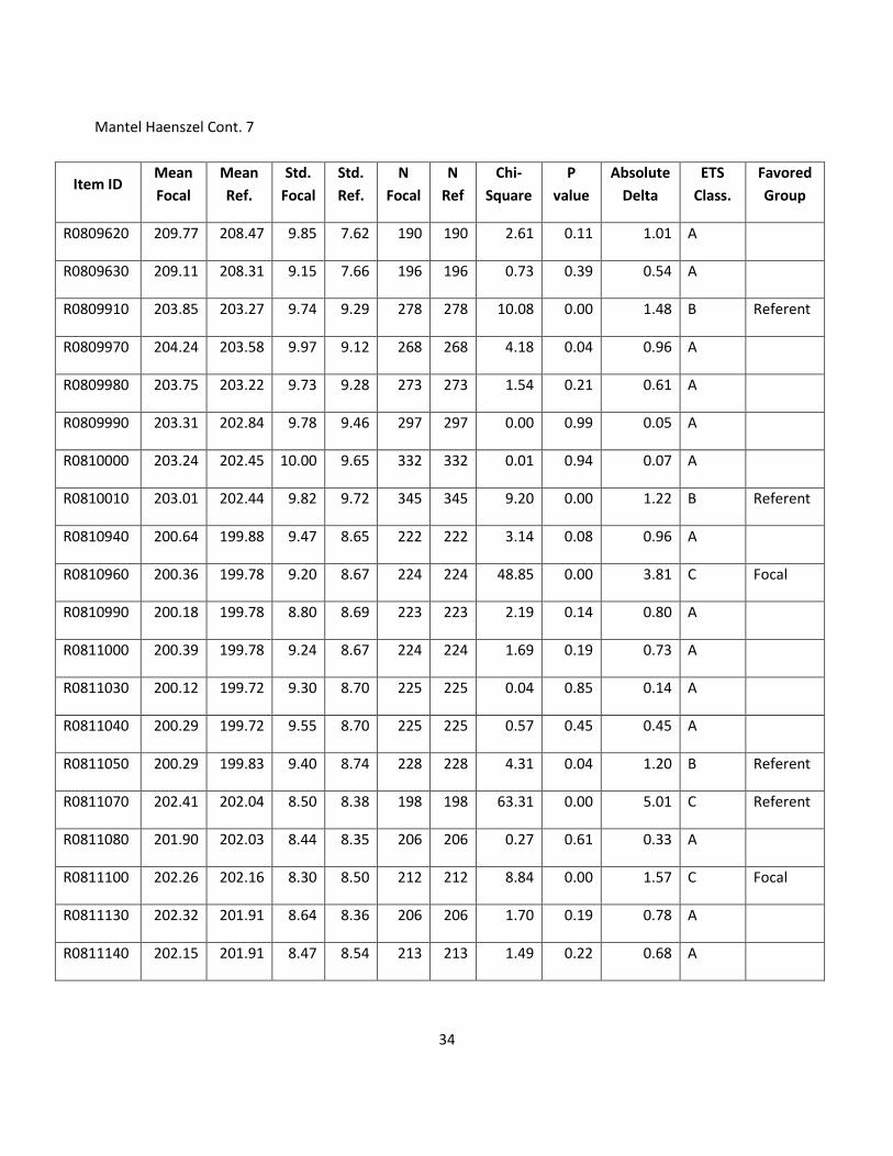
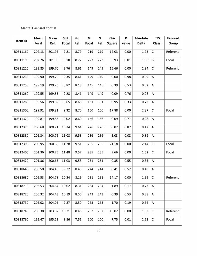
English reading pools. Mantel Haenszel results are rated using a classification system adopted by
Educational Testing Systems (ETS) and developed by Zieky (1993). Items with large DIF are rated C, items
with moderate DIF are rated B, and all other items with little or no DIF are rated A. ETS recommends that
all C items be evaluated and considered for removal.
Although some of the items from the Spanish pools had less than 200 responses, the decision was made to
be cautious and analyze every item no matter what the number of responses. There were 169 items
analyzed in this DIF analysis but only 81 items had more than 200 responses. A total of 14 items had at
least 200 cases in each group and received C ratings – 8 items had results favoring the referent group while
6 items had results favoring the focal group. The 14 items represented about 7 percent of the item pool.
Another 17 items received B ratings and the remaining items received A ratings. Schultz and Geisinger
(1992) found that the agreement between the logistic regression and the Mantel Haenszel procedure
declines with decreased sample size or when the number of levels employed by the Mantel Haenszel is less
than 10.
As recommended by Jodoin and Gierl (2001), items possessing moderate or large amounts of non-uniform
DIF, uniform DIF, or both uniform and uniform DIF were analyzed. Logistic regression produced 7
significant DIF results for items with at least 200 responses in each group, and all 7 of these items also had
some form of uniform DIF and were also identified in the Mantel Haenszel analysis. However, the severity
of the DIF was less than the severity of the DIF identified by Mantel-Haenszel. Using the Jodoin and Gierl
(2001) effect size criteria, of the 7 items demonstrating DIF, 6 had moderate DIF and 1 had large DIF.
Logistic regression appeared to indicate more moderate DIF since, often times, DIF estimated as large and
uniform in the Mantel Haenszel odds ratios migrated to the interaction term in the logistic regression.
Although the uniform tests for the items in Table 5 on the next were still significant, the effect sizes
decreased in a manner that changed their classifications to No DIF. Moreover, even if one accepts only the
Mantel Haenszel results, only 8 of the items favor the referent group.

18
DIF Results
Table 5
Item ID Mantel Haenszel Logistic Regression Group Favored Dropped
R0208500 C No DIF Referent
R0812400 C No DIF Focal
R0812390 C No DIF Focal X
R0237330 C No DIF Referent
R0242390 C No DIF Referent
R0818680 C No DIF Referent
R0811160 C No DIF Referent
R0716330 C Moderate Focal X
R0802840 C Moderate Referent
R0470030 B Moderate Referent
R0819070 B Moderate Focal
R0818740 C Moderate Referent
R0811100 C Moderate Focal X
R0810960 C Large Focal
A total of 165 of the 169 Spanish items had large score effects (Nagelkerke 0.07 and p-value 0.01)
suggesting that they were highly related to the latent trait of interest. Almost 98 percent of the Spanish
items in the pools had Nagelkerke coefficients of determination associated with the Spanish scale score
that exceeded 0.07. Almost half (47%) of the Spanish items had coefficients of determination of 0.20 or
greater. This finding suggests that most of the items in the Spanish pool had high convergent validity with
the latent trait.
Three of the thirteen items with C ratings were rejected for future administration by content specialists and
translators based largely upon translation differences in some word or phrase in the item’s language
complexity between the English and Spanish versions. Two additional items with less than 200 responses
were also rejected for the same reasons. One item favored the focal group and a second favored the
referent group.

19
Classification Accuracy Results
A comparison of the Spanish and English results is first performed using scores generated with Spanish and
English item calibrations. Using item response data from the Spanish pool, if the Spanish calibrations
generate systematically different scores then scores produced by English calibrations, the item calibrations
are not comparable because the resulting scores are different.
Ability Score Comparison
Figure 3
The average scale scores and their respective standard deviations are presented in Table 6.
No matter whether the scale scores are calculated with Spanish or English calibrations, results are
very comparable. A scatter plot of this result can be seen in Figure 3. Scores appear to be very
linear, with a correlation of 0.996. This result suggests that the calibrations produced for English
Reading items are useful for producing comparable results on the Spanish Reading test.
Average Scale Score Calculations for Spanish Items calibrated Two Ways
Table 6
Type of Calibration Mean θ Std Dev θ
Spanish Calibrated 200.378 9.20
English Calibrated 200.365 9.5

20
The RIT scale scores produced with the different Spanish and English item calibrations
demonstrated high levels of classification agreement when the grade 3 performance standard was
applied. In Table 6, 95.9 (54.4 +41.5=95.9) percent of the scores produced by the two different sets
of item calibrations reliably classified the scores.
Observed Scores (Spanish Calibrations) to Observed Scores (English Calibrations)
Table 7
Spn. Observed\Eng. Observed Does Not Meet Observed Meets Observed
Does Not Meet Observed 465 (54.4%) 13 (1.5%)
Meets Observed 22 (2.5%) 355 (41.5%)
Tables 7 and 8 below present the observed and expected number of examinees and their
percentages using the latent distribution method. Results of the classification analysis suggest an
estimated classification accuracy of 89.1 percent (50.9%+38.2%) for the Spanish Reading Test when
compared to the latent distribution.
Observed Spanish Reading Scores (Spanish Calibrations) to the Latent Expected Scores
Table 8
Observed\Expected Does Not Meet Expected Meets Expected
Does Not Meet Observed 435 (50.9%) 47 (5.5%)
Meets Observed 46 (5.4%) 327 (38.2%)
A comparable rate of 90.5% (52.5%+38%) accuracy classification was observed for the Spanish
Reading Test using English calibrations. These results suggest good agreement at reaching an
accurate decision using either set of calibrations when classifying students with the performance
standard.
Observed Spanish Reading Scores (English Calibrations) to the Latent Expected Scores
Table 9
Observed\Expected Does Not Meet Expected Meets Expected
Does Not Meet Observed 449 (52.5%) 51 (6%)
Meets Observed 30 (3.5%) 325 (38%)
21
Conclusions
Validity and reliability claims are typically based on the score interpretations users will make when
making inferences regarding some specified test purpose (Kane, 2006; Messick, 1989). If the
decision maker’s desire is to make comparable decisions with English and Spanish test scores that
are perfectly equivalent, then the stronger levels of parallel testing need to be met.
Interchangeable true score could only be produced when two forms are perfectly parallel, but in
many testing situations a form of comparability can be achieved when the same target is measured
with small differences in reliability. Wu, Li, and Zumbo (2006) found similar effects in TIMMS data
only in countries with the same language. Countries testing with different languages often could
not attain congeneric equivalence between translations of their tests and English.
The current study examines English and Spanish Reading data over comparative definitions of test
equivalence using multiple-group CFA. Results of a CFA study demonstrated essential tau-
equivalent scores that permit users to make decisions about scores that are on the same scale as
the English Reading test and have the same factor structure. Although the mean precision and
errors in measurement may differ between the Spanish and English scales, these differences appear
to be small in actual effect when considering the CFA and DIF results.
Great efforts were made to create over 200 comparable items in both English and Spanish for test
use. Of these items, 169 were used in this first field test of Spanish Reading. For items with 200 or
more responses in Spanish, large differences in item functioning were only observed for 13 items,
and these differences equally favored both groups. Such results compare quite variability with
similar DIF studies of forms translated into different languages (see Sereci & Khaliq, 2002, Gierl &
Khaliq, 2001; Ercikan & Kohl, 2005). In fact, the logistic regression results suggested more moderate
DIF was present than large DIF, and Mantel Haenszel tests produced only 8 large DIF items that
favored English speakers. Content specialists and translators continue to monitor these items to
improve on the translation or adaption of the item into a second language.
When making decisions using the performance standard, both the English and Spanish Reading
calibrations produced comparable results when making decisions with the scores with Oregon
performance standards.
Although these effects were not studied, random forms produced by computer adaptive tests
might produce greater between form comparability than the standard fixed forms used in paper
and pencil testing. Likewise, the use of linguistic experts might also help to reduce language
differences in items. Future research in these areas in needed.

22
References
Browne, M.W. , & Cudek, R. (1993). Alternative ways of assessing model fit. In K. A. Bollen & J. S.
Long (Eds.) Testing structural equations models (pp. 445-455). Newbury Park, CA: Sage.
Chueng, G.W., & Rensvold, R.B. (2002). Evaluating goodness-of-fit indexes for testing MI.
Structural Equation Modeling, 9, 235-255.
Dorans, N.J., & Holland, P.W. (1993). DIF detection and description: Mantel Haenszel and
standardization. In P.W. Holland & H. Wainer (Eds.). Differential item functioning (pp. 35-66).
Hillsdale, NJ: Lawrence Erlbaum Associates.
Camilli, G. (2006). Test fairness. In R. Brennan (Ed.), Educational Measurement (4th ed. pp.187-220).
Westport, CT: Greenwood Publishing.
Ericikan, K., & Koh, K. (2005). Examining the construct comparability of the English and French
versions of TIMSS. International Journal of Testing, 5, 23-35.
Feldt, L.S. & Brennan, R.L. (1989). Reliability. In R.L. Linn (Ed.) Educational measurement (3rd ed.,
105-146). New York: American Council on Education and Macmillan.
Gierl, M. J., & Khaliq, S.N. (2001). Identifying sources of differential item and bundle functioning on
translated achievement tests: A confirmatory analysis. Journal of Education Measurement, 38,
164-187.
Graham, J.M. (2006). Congeneric and (essentially) tau-equivalent estimates of score reliability.
Educational and Psychological Measurement, 66, 6, 930-944.
Guo, F. (2006). Expected classification accuracy using latent distributions. GMAC Research Reports.
June 1, 2006.
Hambleton, R.K. (1994). Guidelines for adapting educational and psychological tests: A progress
report. European Journal of Psychological Assessment, 10, 229-244.
Holland, P.W., & Wainer, H (Eds.). (1993). Differential item functioning. Hillsdale, NJ: Lawrence
Erlbaum Associates.
Kane, M.T. Validation. In R. Brennan (Ed.), Educational Measurement ( 4th ed., pp. 17-64).
Westport, CT: Greenwood Publishing.

23
Jodoin, M.G., & Gierl, M.J. (2001). Evaluating power and type I error rates using an effect size with
the logistic regression procedure for DIF. Applied Measurement in Education, 14, 329-349.
Messick, S. (1989). Validity. In R.L. Linn (Ed.) Educational measurement (3rd ed., 13-103). New
York: American Council on Education and Macmillan.
Raykov, T. (1997b). Scale reliability, Cronbach’s coefficient alpha, and violations of essential tau equivalence with fixed congeneric components. Multivariate Behavioral Research, 32, 329-353.
Rudner, L.M. (2001). Computing the expected proportions of misclassified examinees. Practical
Assessment Research and Evaluation, 7(14).
Sireci, S. G. & Khaliq, S.N. (2002, April). An analysis of the psychometric properties of the dual
language test forms. Paper presented at the annual meeting of the National Council on
Measurement in Education, New Orleans, LA.
Schultz, M.T., & Geisinger, K.F. (1992). The effect of sample size and matching strategy on Mantel
Haenszel and logit DIF procedures. Paper presented at the Annual Meeting of the National
Council on Measurement in Education (San Francisco, CA).
Vandenberg, R.J. & Lance C.E. (2000). A review and synthesis of the MI literature: Suggestions,
practices, recommendations for organizational research. Organizational Research Methods, 3,
4-69.
Van de Viver, F.J. R & Hambleton, R. K. (1996). Translating tests: some practical guidelines. European Psychologist, 1 (2), pp. 89-99.
Wu, Li, & Zumbo (2006). Decoding the meaning of factor invariance and updating the practice of
multigroup confirmatory factor analysis. Practical Assessment and Research Evaluation, 12, 3, 1-
26.
Zieky, M.(1993). Practical questions in the use of DIF statistics in test development. . In P.W.
Holland & H. Wainer (Eds.). Differential item functioning (pp. 337-347). Hillsdale, NJ: Lawrence
Erlbaum Associates.
Zumbo, B.D. (1999). A handbook on the theory and methods of differential item functioning:
Logistic regression modeling as a unitary framework for binary and Likert-type (ordinal) item
scores. Ottawa, On.: Directorate of Human Resources Research and Evaluation, Department of
Defense.

24
Appendix A
Differential Item Functioning Statistics

25
Glossary
Mantel Haenszel Table Headings
Mean Focal : The average scale score for all persons comprising the protected group that may be
adversely affected by the test. In this case, students taking reading items in Spanish are being
treated as the focal group.
Mean Referent (Mean Ref.): The average scale score of all other persons not under protected status
whose scores are matched to the focal group. In this case, students with comparable overall scale
scores taking the English reading test are included in the referent group.
Standard deviation of the Focal group (Std. Focal): the square root of the average squared
deviation of each score from the mean for each member of the focal group. The standard deviation
tells you how tightly the various scores are clustered around the mean in a set of data.
Standard deviation of the Referent group (Std. Referent): the square root of the average squared
deviation of each score from the mean for each member of the referent group. The matching
routine was written to reproduce a similar distribution for the referent group. Therefore, the
standard deviations for both groups should be roughly equal.
Number Focal (N Focal): The number of students classified as members of the focal group.
Number Referent (N Refer.): The number of students classified as members of the referent group.
Mantel Haenszel Chi-Squre (MH Chi-sq): A calculated test of significance based on the common
odds ratio. The total test scores for students in each group are classified into 10 intervals and a 2x2
table is formed for each table. A chi-square is then calculated for each table and summed, so the
number of degrees of freedom is the number of intervals. The calculated chi-square tests whether
the two groups answer in similar ways across all levels of the matching criterion.
Mantel Haneszel P-value (MH P value): The probability that the value of a chi-square statistic can be
greater than the chi-square value we calculated. If the p value is less than the specified p-value
(typically .05 or .01), then we reject the null hypothesis of no difference between the groups and
conclude that there is some difference.
Absolute Delta: The absolute value of delta D DIF and a measure of effect. Delta D DIF (not
displayed in the table) describes a transformation of the odds ratio that makes the distribution
symmetric about 0. If the value of Delta D DIF is negative, the focal group finds the item to be
26
easier. If the value of Delta DIF is positive, the referent group finds the item to be easier. When
the absolute value is calculated, the ETS classification system can be applied to the effect.
ETS Classification: A rating of A, B, or C based on a significant p-value and the magnitude of
absolute delta using the Mantel Haensel Test. If the absolute value of delta is equal to or larger
than 1.0 and less than 1.5, there is moderate DIF. If the absolute value of delta is equal to or great
than 1.5, there is large DIF.
Favored Group: The group favored by the item as identified by the Mantel Haenszel test.
Logistic Regression Table Headings
Uniform Chi-Square: A chi-square statistic measuring modeled change over and above any real
score differences attributed to the latent trait. A significant Chi-square value suggests that one
group is outperforming the other group in an even fashion across the ability distribution, and that
these nuisance differences are not explained by the latent trait being measured.
Uniform P-value: The probability that the value of the chi-square statistic is greater than the
obtained value of the chi-square statistic associated with the group effect. Again, a p-value less
than 0.05 suggests that the null hypothesis can be rejected and that there are significant group
differences in the probability of the response.
Uniform Effects (Uniform Change): Changes in the Nagelkerke R 2 associated with uniform effects
greater than 0.035. The effect difference is less sensitive to changes in sample size, so it is valuable
in this context. Moderate effects have a Nagelkerke R 2 equal to or greater than 0.035 and less than
0.07 with a p-values less than or equal to 0.05. Large effects have a Nagelkerke R 2 equal to or
greater than 0.07 with p-value less than or equal to 0.05.
Non-Uniform Chi-Square: A chi-square statistic measuring the score-by-group interaction over and
above any real score or uniform differences. In other words, an interaction effect benefits one
group in one part of the score distribution while another group benefits in a different area of the
score distribution.
Non-Uniform P-value: The probability that the value of the chi-square statistic is greater than the
obtained value of the chi-square statistic associated with the group by score interaction. Again, a
p-value less than 0.05 suggests that the null can be rejected and that there are significant
confounding differences in the probability of the group response.
Non-Uniform effects (Interaction Change): Changes in the Nagelkerke R 2 associated with non-
uniform effects. The effect difference is less sensitive to changes in sample size, so it is valuable in

27
this context. Moderate effects have a Nagelkerke R 2 equal to or greater than 0.035 and less than
0.07 with a p-values less than or equal to 0.05. Large effects have a Nagelkerke R 2 equal to or
greater than 0.07 with p-value less than or equal to 0.05.
Jodoin/Gierl Classification: A rating of DIF based upon the p-value and the magnitude of the effect
associated with either the uniform or interaction models. The Jodoin-Gierl (2001) effect size criteria
are:
Negligible or A-level DIF: R2 < 0.035
Moderate or B-level DIF: Null hypothesis rejected and 0.035 < R2 < 0.070
Large or C-level DIF: Null hypothesis rejected and R2 > 0.070

28
Mantel-Haenszel Statistics
Item ID Mean
Focal
Mean
Ref.
Std.
Focal
Std.
Ref.
N
Focal
N
Ref
MH
Chi-Sq
MH
P value
Absolute
Delta
ETS
Class.
Favored
Group
R0208430 208.99 207.53 9.88 7.84 187 187 0.84 0.36 0.56 A
R0208440 208.37 207.52 8.66 7.99 190 190 0.14 0.71 0.28 A
R0208450 208.59 207.18 10.63 8.00 200 200 0.22 0.64 0.33 A
R0208480 207.79 206.35 9.82 8.35 218 218 0.00 0.98 0.05 A
R0208500 207.90 206.56 9.86 8.16 218 218 8.35 0.00 1.48 B Referent
R0224210 206.02 205.57 9.38 8.51 246 246 1.31 0.25 0.73 A
R0224220 207.02 206.17 9.10 8.29 223 223 1.03 0.31 0.63 A
R0224240 206.54 206.17 8.58 8.29 223 223 1.41 0.23 0.63 A
R0224250 195.90 196.21 9.04 8.38 129 129 0.03 0.87 0.19 A
R0224930 201.94 201.37 9.94 8.65 212 212 5.44 0.02 1.55 C Referent
R0224940 201.80 201.37 9.45 8.65 212 212 1.41 0.23 0.68 A
R0224980 203.67 202.83 10.37 8.79 275 275 6.12 0.01 1.18 B Referent
R0237300 198.35 198.01 10.36 9.89 243 243 1.75 0.19 0.73 A
R0237310 197.87 197.71 10.39 9.90 234 234 0.00 0.96 0.07 A
R0237330 198.02 197.81 10.09 9.83 243 243 7.44 0.01 1.55 C Referent
R0237430 195.92 195.94 9.12 8.34 127 127 2.47 0.12 1.27 A
R0237440 195.81 196.24 9.45 8.46 130 130 0.00 0.97 0.12 A
R0237450 196.46 196.38 9.22 8.50 133 133 3.05 0.08 1.34 A
R0237470 196.70 196.60 10.21 8.52 138 138 0.01 0.92 0.28 A
R0237510 196.59 196.67 9.23 8.54 140 140 0.24 0.62 0.40 A
29
Mantel Haenszel Cont. 2
Item ID Mean
Focal
Mean
Ref.
Std.
Focal
Std.
Ref.
N
Focal
N
Ref
Chi-
Square
P
value
Absolute
Delta
ETS
Class.
Favored
Group
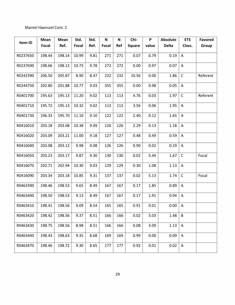
R0237650 198.44 198.14 10.99 9.81 271 271 0.07 0.79 0.19 A
R0237690 198.66 198.12 10.73 9.78 272 272 0.00 0.97 0.07 A
R0242390 206.50 205.87 8.90 8.47 232 232 10.56 0.00 1.86 C Referent
R0244750 202.80 201.88 10.77 9.03 355 355 0.00 0.98 0.05 A
R0401700 195.63 195.13 11.20 9.02 113 113 4.76 0.03 1.97 C Referent
R0401710 195.72 195.13 10.32 9.02 113 113 3.56 0.06 1.95 A
R0401730 196.33 195.70 11.10 9.10 122 122 2.40 0.12 1.65 A
R0416010 203.18 203.08 10.38 9.09 126 126 2.29 0.13 1.18 A
R0416020 203.09 203.21 11.00 9.18 127 127 0.48 0.49 0.59 A
R0416040 203.08 203.12 9.98 9.08 126 126 0.90 0.02 0.19 A
R0416050 203.23 203.17 9.87 9.30 130 130 0.02 5.44 1.67 C Focal
R0416070 202.71 202.94 10.30 9.03 129 129 0.30 1.08 1.13 A
R0416090 203.34 203.18 10.85 9.31 137 137 0.02 5.13 1.74 C Focal
R0463390 198.46 198.53 9.65 8.49 167 167 0.17 1.85 0.89 A
R0463400 198.50 198.53 9.13 8.49 167 167 0.17 1.91 0.94 A
R0463410 198.41 198.56 9.09 8.54 165 165 0.91 0.01 0.00 A
R0463420 198.42 198.56 9.37 8.51 166 166 0.02 5.03 1.48 B
R0463430 198.75 198.56 8.98 8.51 166 166 0.08 3.09 1.13 A
R0463440 198.43 198.63 9.35 8.68 169 169 0.99 0.00 0.09 A
R0463470 198.46 198.72 9.30 8.65 177 177 0.92 0.01 0.02 A
30
Mantel Haenszel Cont. 3
Item ID Mean
Focal
Mean
Ref.
Std.
Focal
Std.
Ref.
N
Focal
N
Ref
Chi-
Square
P
value
Absolute
Delta
ETS
Class.
Favored
Group
R0470030 208.78 207.57 9.75 7.38 215 215 0.01 7.06 1.46 B Referent
R0470060 208.69 207.57 9.64 7.38 215 215 0.75 0.10 0.26 A
R0470070 208.73 207.62 9.32 7.37 219 219 0.72 0.13 0.24 A
R0477360 197.14 196.37 10.74 8.60 161 161 0.55 0.35 0.45 A
R0477370 196.73 196.27 10.18 8.44 191 191 0.21 1.60 0.82 A
R0477380 196.67 196.27 10.13 8.44 191 191 0.94 0.01 0.02 A
R0477400 197.04 196.54 10.55 8.57 197 197 0.96 0.00 0.05 A
R0506810 193.78 193.75 8.50 7.64 246 246 0.00 7.91 1.46 B Focal
R0506820 194.02 193.75 8.89 7.64 248 248 0.03 4.83 1.08 B Focal
R0506840 193.67 193.68 8.88 7.65 248 248 0.01 6.02 1.22 B Focal
R0506870 193.27 193.68 8.93 7.68 249 249 0.00 8.00 1.41 B Focal
R0506880 193.60 193.77 9.38 7.67 253 253 0.81 0.06 0.16 A
R0517630 201.61 200.93 10.45 9.46 350 350 0.08 3.01 0.75 A
R0517650 200.24 200.27 9.21 8.97 284 284 0.06 3.66 0.94 A
R0517670 200.11 200.27 8.93 8.97 284 284 0.25 1.31 0.61 A
R0517680 201.04 200.88 9.40 9.10 308 308 0.05 3.82 0.92 A
R0705570 196.46 196.68 9.00 8.32 108 108 0.00 12.68 2.68 C Focal
R0705580 196.60 196.68 9.24 8.32 108 108 0.60 0.27 0.56 A
R0705590 196.96 196.76 9.25 8.33 109 109 0.73 0.12 0.35 A
R0705600 196.98 196.66 9.81 8.29 108 108 0.79 0.07 0.35 A
31
Mantel Haenszel Cont. 4
Item ID Mean
Focal
Mean
Ref.
Std.
Focal
Std.
Ref.
N
Focal
N
Ref
Chi-
Square
P
value
Absolute
Delta
ETS
Class.
Favored
Group
R0705630 197.10 196.82 9.75 8.24 113 113 0.12 2.43 1.46 A
R0705640 197.26 197.12 10.21 8.35 117 117 0.32 0.97 0.89 A
R0705660 197.49 197.40 9.07 8.41 121 121 0.54 0.38 0.63 A
R0705820 193.76 193.15 10.23 8.69 54 54 0.92 0.01 0.19 A
R0705840 192.59 193.15 8.68 8.69 54 54 0.65 0.21 0.85 A
R0705850 193.50 193.15 10.35 8.69 54 54 0.91 0.01 0.21 A
R0705860 194.27 193.73 10.10 8.61 59 59 0.09 2.96 2.44 A
R0716330 201.43 201.01 10.18 9.27 316 316 0.00 21.53 2.09 C Focal
R0716350 201.53 200.98 9.98 9.32 324 324 0.54 0.37 0.31 A
R0716360 201.31 201.06 9.56 9.29 310 310 0.75 0.10 0.16 A
R0716380 201.22 200.61 10.05 9.49 325 325 0.57 0.45 0.33 A
R0716400 200.98 200.56 9.90 9.48 328 328 7.48 0.01 1.15 B Referent
R0716410 200.87 200.52 9.92 9.62 337 337 0.11 0.74 0.16 A
R0719360 202.39 202.09 9.02 8.53 127 127 0.69 0.41 0.66 A
R0719370 202.15 202.07 9.13 8.56 123 123 0.94 0.33 0.85 A
R0719380 201.87 201.89 9.41 8.74 129 129 5.84 0.02 1.76 C Referent
R0719410 202.02 201.78 9.27 8.73 133 133 0.95 0.33 0.75 A
R0719430 201.72 201.81 9.07 8.74 145 145 0.37 0.54 0.47 A
R0719460 202.23 201.65 9.70 8.75 160 160 26.41 0.00 3.50 C Focal
R0802570 193.67 194.08 8.68 8.34 95 95 0.98 0.32 0.96 A

32
Mantel Haenszel Cont. 5
Item ID Mean
Focal
Mean
Ref.
Std.
Focal
Std.
Ref.
N
Focal
N
Ref
Chi-
Square
P
value
Absolute
Delta
ETS
Class.
Favored
Group
R0802590 194.47 194.36 8.45 8.36 98 98 0.42 0.52 0.85 A
R0802600 193.65 194.16 8.91 8.33 96 96 0.27 0.60 0.75 A
R0802610 194.19 194.32 8.80 8.35 100 100 0.02 0.89 0.28 A
R0802630 194.33 194.35 8.62 8.30 106 106 0.42 0.52 0.63 A
R0802660 194.60 194.69 8.88 8.23 115 115 2.33 0.13 1.39 A
R0802670 197.45 197.11 8.92 8.42 184 184 1.48 0.22 0.75 A
R0802690 197.19 197.06 9.21 8.43 186 186 4.30 0.04 1.15 B Focal
R0802700 197.18 197.02 8.49 8.34 179 179 0.06 0.81 0.21 A
R0802720 197.44 196.99 9.31 8.39 185 185 1.72 0.19 0.80 A
R0802740 196.99 196.90 9.34 8.32 187 187 0.30 0.58 0.40 A
R0802760 197.39 196.99 9.32 8.35 197 197 0.08 0.78 0.24 A
R0802770 197.64 197.26 9.17 8.38 205 205 0.00 1.00 0.07 A
R0802780 198.13 198.12 10.17 9.47 291 291 4.94 0.03 1.03 B Referent
R0802810 198.17 197.62 10.20 9.38 268 268 0.26 0.61 0.31 A
R0802830 197.91 197.70 10.58 9.37 286 286 0.02 0.88 0.12 A
R0802840 198.42 197.94 9.85 9.34 303 303 19.43 0.00 2.12 C Referent
R0802850 198.23 198.09 9.90 9.47 311 311 2.31 0.13 0.68 A
R0808960 195.53 195.15 8.36 7.47 185 185 0.11 0.74 0.24 A
R0808980 195.47 195.13 8.84 7.50 181 181 2.31 0.13 0.92 A
R0809010 195.39 195.16 8.14 7.48 184 184 3.69 0.05 1.15 B Referent

33
Mantel Haenszel Cont. 6
Item ID Mean
Focal
Mean
Ref.
Std.
Focal
Std.
Ref.
N
Focal
N
Ref
Chi-
Square
P
value
Absolute
Delta
ETS
Class.
Favored
Group
R0809020 195.72 195.12 8.27 7.46 187 187 32.11 0.00 3.34 C Referent
R0809030 195.59 195.31 7.88 7.51 196 196 0.56 0.46 0.49 A
R0809050 195.44 195.38 8.09 7.53 198 198 0.11 0.74 0.26 A
R0809330 204.60 204.05 10.23 9.60 266 266 6.89 0.01 1.25 B Focal
R0809340 204.60 204.02 9.79 9.57 258 258 6.27 0.01 1.22 B Referent
R0809350 204.55 203.79 10.16 9.88 270 270 1.87 0.17 0.63 A
R0809380 204.64 203.81 10.41 9.96 280 280 10.75 0.00 1.46 B Referent
R0809400 204.26 203.64 10.27 10.00 289 289 0.78 0.38 0.45 A
R0809410 204.10 203.44 9.94 9.91 306 306 2.17 0.14 0.66 A
R0809440 197.48 197.31 8.97 8.48 189 189 3.57 0.06 1.06 A
R0809450 197.75 197.49 9.20 8.58 192 192 0.32 0.57 0.38 A
R0808980 197.76 197.33 9.13 8.48 187 187 0.00 0.95 0.12 A
R0809480 197.72 197.57 9.11 8.64 190 190 0.02 0.88 0.14 A
R0809520 197.77 197.58 8.81 8.64 196 196 9.49 0.00 1.83 C Referent
R0809530 197.77 197.69 9.41 8.48 206 206 0.10 0.75 0.24 A
R0809550 208.76 208.58 8.60 7.58 187 187 26.93 0.00 2.77 C Referent
R0809570 209.40 208.56 9.27 7.56 188 188 0.09 0.76 0.24 A
R0809590 209.31 208.67 8.46 7.50 186 186 0.05 0.83 0.19 A
R0809600 209.94 208.65 9.25 7.48 187 187 3.13 0.08 1.13 A
R0809610 209.34 208.68 9.06 7.47 188 188 18.76 0.00 2.44 C Focal
34
Mantel Haenszel Cont. 7
Item ID Mean
Focal
Mean
Ref.
Std.
Focal
Std.
Ref.
N
Focal
N
Ref
Chi-
Square
P
value
Absolute
Delta
ETS
Class.
Favored
Group
R0809620 209.77 208.47 9.85 7.62 190 190 2.61 0.11 1.01 A
R0809630 209.11 208.31 9.15 7.66 196 196 0.73 0.39 0.54 A
R0809910 203.85 203.27 9.74 9.29 278 278 10.08 0.00 1.48 B Referent
R0809970 204.24 203.58 9.97 9.12 268 268 4.18 0.04 0.96 A
R0809980 203.75 203.22 9.73 9.28 273 273 1.54 0.21 0.61 A
R0809990 203.31 202.84 9.78 9.46 297 297 0.00 0.99 0.05 A
R0810000 203.24 202.45 10.00 9.65 332 332 0.01 0.94 0.07 A
R0810010 203.01 202.44 9.82 9.72 345 345 9.20 0.00 1.22 B Referent
R0810940 200.64 199.88 9.47 8.65 222 222 3.14 0.08 0.96 A
R0810960 200.36 199.78 9.20 8.67 224 224 48.85 0.00 3.81 C Focal
R0810990 200.18 199.78 8.80 8.69 223 223 2.19 0.14 0.80 A
R0811000 200.39 199.78 9.24 8.67 224 224 1.69 0.19 0.73 A
R0811030 200.12 199.72 9.30 8.70 225 225 0.04 0.85 0.14 A
R0811040 200.29 199.72 9.55 8.70 225 225 0.57 0.45 0.45 A
R0811050 200.29 199.83 9.40 8.74 228 228 4.31 0.04 1.20 B Referent
R0811070 202.41 202.04 8.50 8.38 198 198 63.31 0.00 5.01 C Referent
R0811080 201.90 202.03 8.44 8.35 206 206 0.27 0.61 0.33 A
R0811100 202.26 202.16 8.30 8.50 212 212 8.84 0.00 1.57 C Focal
R0811130 202.32 201.91 8.64 8.36 206 206 1.70 0.19 0.78 A
R0811140 202.15 201.91 8.47 8.54 213 213 1.49 0.22 0.68 A
35
Mantel Haenszel Cont. 8
Item ID Mean
Focal
Mean
Ref.
Std.
Focal
Std.
Ref.
N
Focal
N
Ref
Chi-
Square
P
value
Absolute
Delta
ETS
Class.
Favored
Group
R0811160 202.13 201.95 9.81 8.79 219 219 12.03 0.00 1.93 C Referent
R0811190 202.26 201.98 9.18 8.72 223 223 5.93 0.01 1.36 B Focal
R0811210 199.85 199.70 9.76 8.61 149 149 16.66 0.00 2.84 C Referent
R0811230 199.90 199.70 9.35 8.61 149 149 0.00 0.98 0.09 A
R0811250 199.19 199.23 8.82 8.18 145 145 0.39 0.53 0.52 A
R0811260 199.55 199.55 9.28 8.41 149 149 0.09 0.76 0.28 A
R0811280 199.56 199.82 8.65 8.68 151 151 0.95 0.33 0.73 A
R0811300 199.91 199.81 9.32 8.70 150 150 17.88 0.00 2.87 C Focal
R0811320 199.87 199.86 9.02 8.60 156 156 0.09 0.77 0.28 A
R0812370 200.68 200.71 10.34 9.64 226 226 0.02 0.87 0.12 A
R0812380 201.34 200.72 11.08 9.58 236 236 3.03 0.08 0.89 A
R0812390 200.95 200.68 11.28 9.51 265 265 21.18 0.00 2.14 C Focal
R0812400 201.36 200.75 11.48 9.57 235 235 9.66 0.00 1.62 C Focal
R0812420 201.36 200.63 11.03 9.58 251 251 0.35 0.55 0.35 A
R0818640 205.50 204.46 9.72 8.45 244 244 0.41 0.52 0.40 A
R0818680 205.53 204.78 10.34 8.19 231 231 14.17 0.00 1.95 C Referent
R0818710 205.53 204.64 10.02 8.31 234 234 1.89 0.17 0.73 A
R0818720 205.32 204.43 10.19 8.50 243 243 0.39 0.53 0.38 A
R0818730 205.02 204.05 9.87 8.50 263 263 1.70 0.19 0.66 A
R0818740 205.38 203.87 10.71 8.46 282 282 15.02 0.00 1.83 C Referent
R0818760 195.47 195.23 8.86 7.51 100 100 7.75 0.01 2.61 C Focal

36
37
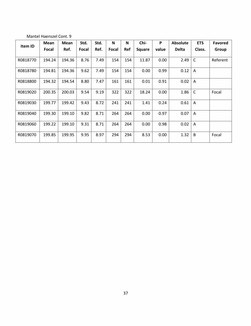
Mantel Haenszel Cont. 9
Item ID Mean
Focal
Mean
Ref.
Std.
Focal
Std.
Ref.
N
Focal
N
Ref
Chi-
Square
P
value
Absolute
Delta
ETS
Class.
Favored
Group
R0818770 194.24 194.36 8.76 7.49 154 154 11.87 0.00 2.49 C Referent
R0818780 194.81 194.36 9.62 7.49 154 154 0.00 0.99 0.12 A
R0818800 194.32 194.54 8.80 7.47 161 161 0.01 0.91 0.02 A
R0819020 200.35 200.03 9.54 9.19 322 322 18.24 0.00 1.86 C Focal
R0819030 199.77 199.42 9.43 8.72 241 241 1.41 0.24 0.61 A
R0819040 199.30 199.10 9.82 8.71 264 264 0.00 0.97 0.07 A
R0819060 199.22 199.10 9.31 8.71 264 264 0.00 0.98 0.02 A
R0819070 199.85 199.95 9.95 8.97 294 294 8.53 0.00 1.32 B Focal
38
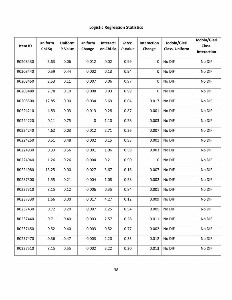
Logistic Regression Statistics
Item ID Uniform
Chi-Sq
Uniform
P-Value
Uniform
Change
Interacti
on Chi-Sq
Inter.
P-Value
Interaction
Change
Jodoin/Gierl
Class. Uniform
Jodoin/Gierl
Class.
Interaction
R0208430 3.63 0.06 0.012 0.02 0.99 0 No DIF No DIF
R0208440 0.59 0.44 0.002 0.13 0.94 0 No DIF No DIF
R0208450 2.53 0.11 0.007 0.06 0.97 0 No DIF No DIF
R0208480 2.78 0.10 0.008 0.03 0.99 0 No DIF No DIF
R0208500 12.85 0.00 0.034 6.69 0.04 0.017 No DIF No DIF
R0224210 4.83 0.03 0.013 0.28 0.87 0.001 No DIF No DIF
R0224220 0.11 0.75 0 1.10 0.58 0.003 No DIF No DIF
R0224240 4.62 0.03 0.012 2.71 0.26 0.007 No DIF No DIF
R0224250 0.51 0.48 0.002 0.15 0.93 0.001 No DIF No DIF
R0224930 0.33 0.56 0.001 1.06 0.59 0.003 No DIF No DIF
R0224940 1.26 0.26 0.004 0.21 0.90 0 No DIF No DIF
R0224980 13.25 0.00 0.027 3.67 0.16 0.007 No DIF No DIF
R0237300 1.55 0.21 0.004 1.08 0.58 0.002 No DIF No DIF
R0237310 8.15 0.12 0.006 0.35 0.84 0.001 No DIF No DIF
R0237330 1.66 0.00 0.017 4.27 0.12 0.009 No DIF No DIF
R0237430 0.72 0.20 0.007 1.25 0.54 0.005 No DIF No DIF
R0237440 0.71 0.40 0.003 2.57 0.28 0.011 No DIF No DIF
R0237450 0.52 0.40 0.003 0.52 0.77 0.002 No DIF No DIF
R0237470 0.36 0.47 0.003 2.20 0.33 0.012 No DIF No DIF
R0237510 8.15 0.55 0.002 3.22 0.20 0.013 No DIF No DIF
39
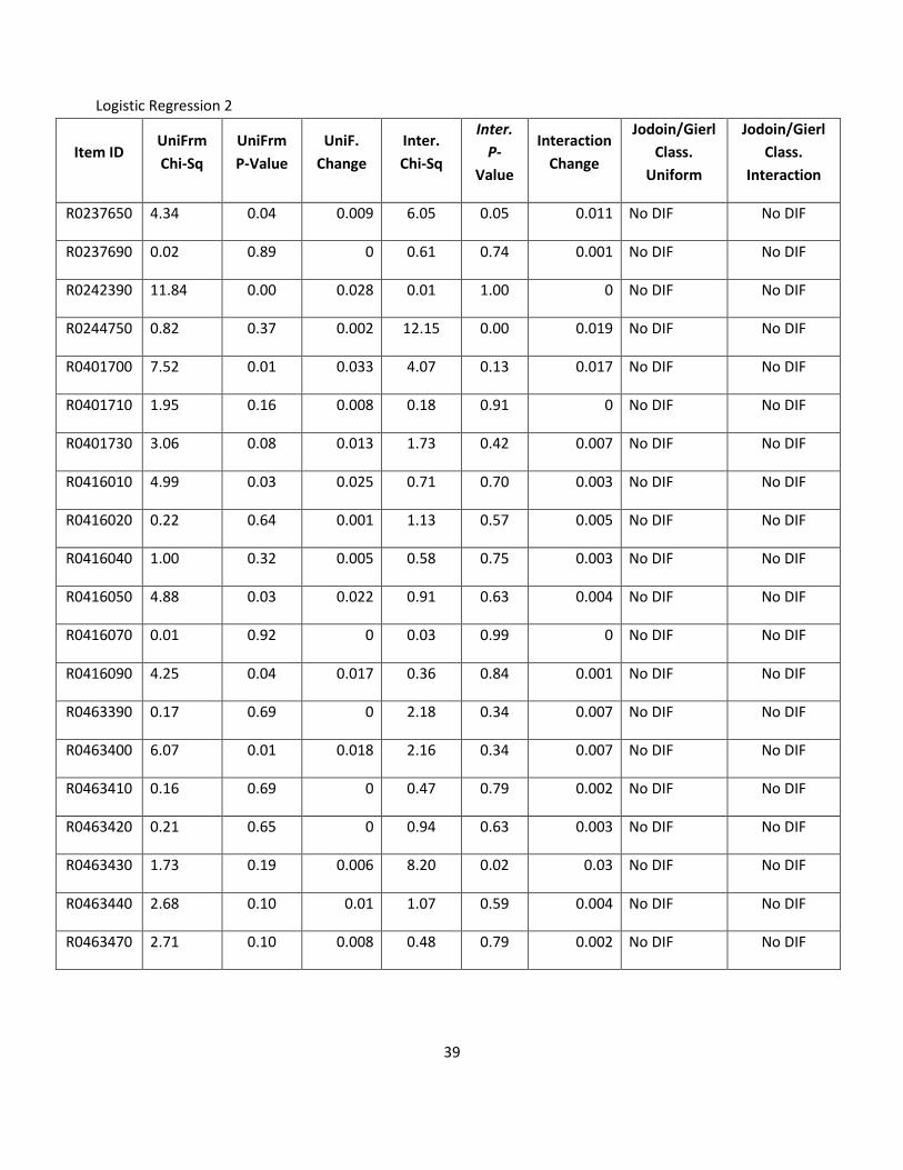
Logistic Regression 2
Item ID UniFrm
Chi-Sq
UniFrm
P-Value
UniF.
Change
Inter.
Chi-Sq
Inter.
P-
Value
Interaction
Change
Jodoin/Gierl
Class.
Uniform
Jodoin/Gierl
Class.
Interaction
R0237650 4.34 0.04 0.009 6.05 0.05 0.011 No DIF No DIF
R0237690 0.02 0.89 0 0.61 0.74 0.001 No DIF No DIF
R0242390 11.84 0.00 0.028 0.01 1.00 0 No DIF No DIF
R0244750 0.82 0.37 0.002 12.15 0.00 0.019 No DIF No DIF
R0401700 7.52 0.01 0.033 4.07 0.13 0.017 No DIF No DIF
R0401710 1.95 0.16 0.008 0.18 0.91 0 No DIF No DIF
R0401730 3.06 0.08 0.013 1.73 0.42 0.007 No DIF No DIF
R0416010 4.99 0.03 0.025 0.71 0.70 0.003 No DIF No DIF
R0416020 0.22 0.64 0.001 1.13 0.57 0.005 No DIF No DIF
R0416040 1.00 0.32 0.005 0.58 0.75 0.003 No DIF No DIF
R0416050 4.88 0.03 0.022 0.91 0.63 0.004 No DIF No DIF
R0416070 0.01 0.92 0 0.03 0.99 0 No DIF No DIF
R0416090 4.25 0.04 0.017 0.36 0.84 0.001 No DIF No DIF
R0463390 0.17 0.69 0 2.18 0.34 0.007 No DIF No DIF
R0463400 6.07 0.01 0.018 2.16 0.34 0.007 No DIF No DIF
R0463410 0.16 0.69 0 0.47 0.79 0.002 No DIF No DIF
R0463420 0.21 0.65 0 0.94 0.63 0.003 No DIF No DIF
R0463430 1.73 0.19 0.006 8.20 0.02 0.03 No DIF No DIF
R0463440 2.68 0.10 0.01 1.07 0.59 0.004 No DIF No DIF
R0463470 2.71 0.10 0.008 0.48 0.79 0.002 No DIF No DIF

40
Logistic Regression 3
Item ID UniFrm
Chi-Sq
UniFrm
P-value Uniform
Change
Inter.
Chi-Sq
Inter.
P-Value Interaction
Change
Jodoin/Gierl
Class.
Uniform
Jodoin/Gierl
Class.
Interaction
R0470030 15.22 0.00 0.042 1.67 0.43 0.005 Moderate No DIF
R0470060 0.29 0.58 0.001 1.09 0.58 0.004 No DIF No DIF
R0470070 0.15 0.70 0 0.20 0.90 0.001 No DIF No DIF
R0477360 6.01 0.01 0.02 0.03 0.99 0 No DIF No DIF
R0477370 1.30 0.25 0.004 0.03 0.99 0 No DIF No DIF
R0477380 0.02 0.89 0 0.01 1.00 0 No DIF No DIF
R0477400 0.03 0.86 0 1.53 0.47 0.004 No DIF No DIF
R0506810 6.78 0.01 0.015 2.95 0.23 0.006 No DIF No DIF
R0506820 7.06 0.01 0.017 0.02 0.99 0 No DIF No DIF
R0506840 12.69 0.00 0.028 5.22 0.07 0.012 No DIF No DIF
R0506870 11.86 0.00 0.029 1.30 0.52 0.004 No DIF No DIF
R0506880 1.99 0.16 0.004 0.00 1.00 0 No DIF No DIF
R0517630 0.67 0.42 0.001 0.41 0.81 0 No DIF No DIF
R0517650 3.25 0.07 0.006 0.05 0.98 0 No DIF No DIF
R0517670 0.23 0.63 0 1.63 0.44 0.003 No DIF No DIF
R0517680 6.21 0.01 0.012 0.31 0.86 0 No DIF No DIF
R0705570 9.82 0.00 0.053 2.29 0.32 0.012 Moderate No DIF
R0705580 0.63 0.42 0.004 0.01 1.00 0 No DIF No DIF
R0705590 3.72 0.05 0.02 0.57 0.75 0.003 No DIF No DIF
R0705600 4.02 0.05 0.025 0.23 0.89 0.001 No DIF No DIF

41
Logistic Regression 4
Item ID Uniform
Chi-Sq
Uniform
P-Value
Uniform
Change
Interaction
Chi-Sq
Inter.
P-Value
Interaction
Change
Jodoin/Gierl
Class.
Uniform
Jodoin/Gierl
Class.
Interaction
R0705630 0.85 0.36 0.003 0.02 0.99 0 No DIF No DIF
R0705640 1.20 0.27 0.006 0.34 0.84 0.001 No DIF No DIF
R0705660 4.15 0.04 0.017 1.56 0.46 0.006 No DIF No DIF
R0705820 0.03 0.86 0 0.06 0.97 0.001 No DIF No DIF
R0705840 0.12 0.73 0.001 3.32 0.19 0.033 No DIF No DIF
R0705850 0.10 0.75 0.001 2.72 0.26 0.027 No DIF No DIF
R0705860 9.28 0.00 0.084 0.28 0.87 0.002 Large No DIF
R0716330 17.62 0.00 0.036 2.76 0.25 0.006 Moderate No DIF
R0716350 1.95 0.16 0.003 6.41 0.04 0.01 No DIF No DIF
R0716360 0.01 0.92 0 0.07 0.97 0 No DIF No DIF
R0716380 3.31 0.07 0.006 0.45 0.80 0.001 No DIF No DIF
R0716400 12.27 0.00 0.023 0.28 0.87 0 No DIF No DIF
R0716410 0.10 0.75 0 0.68 0.71 0.001 No DIF No DIF
R0719360 0.03 0.86 0 0.03 0.99 0 No DIF No DIF
R0719370 0.30 0.58 0.001 2.65 0.27 0.011 No DIF No DIF
R0719380 4.20 0.04 0.018 0.01 1.00 0 No DIF No DIF
R0719410 1.34 0.25 0.006 2.22 0.33 0.008 No DIF No DIF
R0719430 0.74 0.39 0.003 0.55 0.76 0.002 No DIF No DIF
R0719460 23.54 0.00 0.095 4.04 0.13 0.015 Large No DIF
R0802570 5.25 0.02 0.032 1.02 0.60 0.006 No DIF No DIF

42
Logistic Regression 5
Item ID Uniform
Chi-Sq
Uniform
P-Value
Uniform
Change
Interaction
Chi-Sq
Interaction
P-Value
Interaction
Change
Jodoin/Gierl
Class.
Uniform
Jodoin/Gierl
Class.
Interaction
R0802590 1.17 0.28 0.006 2.25 0.32 0.01 No DIF No DIF
R0802600 0.70 0.40 0.003 0.37 0.83 0.002 No DIF No DIF
R0802610 6.03 0.01 0.033 0.53 0.77 0.003 No DIF No DIF
R0802630 6.58 0.01 0.033 3.22 0.20 0.016 No DIF No DIF
R0802660 0.88 0.35 0.004 0.47 0.79 0.002 No DIF No DIF
R0802670 1.52 0.22 0.005 0.89 0.64 0.003 No DIF No DIF
R0802690 9.11 0.00 0.03 21.89 0.00 0.067 No DIF Moderate
R0802700 0.09 0.76 0.001 0.01 1.00 0 No DIF No DIF
R0802720 0.76 0.38 0.002 0.57 0.75 0.002 No DIF No DIF
R0802740 0.51 0.48 0.001 3.29 0.19 0.009 No DIF No DIF
R0802760 0.02 0.89 0 0.82 0.66 0.002 No DIF No DIF
R0802770 0.66 0.42 0.002 0.32 0.85 0.001 No DIF No DIF
R0802780 12.40 0.00 0.022 0.06 0.97 0 No DIF No DIF
R0802810 0.92 0.34 0.001 0.01 1.00 0 No DIF No DIF
R0802830 0.02 0.89 0 0.15 0.93 0 No DIF No DIF
R0802840 19.68 0.00 0.035 3.97 0.14 0.008 Moderate No DIF
R0802850 0.01 0.92 0 0.03 0.99 0 No DIF No DIF
R0808960 0.09 0.76 0 0.01 1.00 0 No DIF No DIF
R0808980 1.63 0.20 0.006 0.01 1.00 0 No DIF No DIF
R0809010 5.25 0.02 0.016 0.54 0.76 0.002 No DIF No DIF
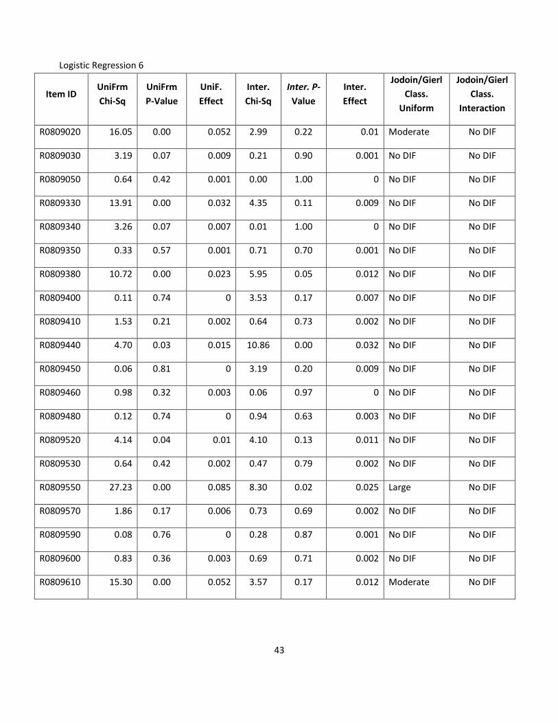
43
Logistic Regression 6
Item ID UniFrm
Chi-Sq
UniFrm
P-Value
UniF.
Effect
Inter.
Chi-Sq
Inter. P-
Value
Inter.
Effect
Jodoin/Gierl
Class.
Uniform
Jodoin/Gierl
Class.
Interaction
R0809020 16.05 0.00 0.052 2.99 0.22 0.01 Moderate No DIF
R0809030 3.19 0.07 0.009 0.21 0.90 0.001 No DIF No DIF
R0809050 0.64 0.42 0.001 0.00 1.00 0 No DIF No DIF
R0809330 13.91 0.00 0.032 4.35 0.11 0.009 No DIF No DIF
R0809340 3.26 0.07 0.007 0.01 1.00 0 No DIF No DIF
R0809350 0.33 0.57 0.001 0.71 0.70 0.001 No DIF No DIF
R0809380 10.72 0.00 0.023 5.95 0.05 0.012 No DIF No DIF
R0809400 0.11 0.74 0 3.53 0.17 0.007 No DIF No DIF
R0809410 1.53 0.21 0.002 0.64 0.73 0.002 No DIF No DIF
R0809440 4.70 0.03 0.015 10.86 0.00 0.032 No DIF No DIF
R0809450 0.06 0.81 0 3.19 0.20 0.009 No DIF No DIF
R0809460 0.98 0.32 0.003 0.06 0.97 0 No DIF No DIF
R0809480 0.12 0.74 0 0.94 0.63 0.003 No DIF No DIF
R0809520 4.14 0.04 0.01 4.10 0.13 0.011 No DIF No DIF
R0809530 0.64 0.42 0.002 0.47 0.79 0.002 No DIF No DIF
R0809550 27.23 0.00 0.085 8.30 0.02 0.025 Large No DIF
R0809570 1.86 0.17 0.006 0.73 0.69 0.002 No DIF No DIF
R0809590 0.08 0.76 0 0.28 0.87 0.001 No DIF No DIF
R0809600 0.83 0.36 0.003 0.69 0.71 0.002 No DIF No DIF
R0809610 15.30 0.00 0.052 3.57 0.17 0.012 Moderate No DIF

44
Logistic Regression 7
Item ID UniFrm
Chi-Sq
UniFrm
P-Value
UniF.
Effect
Inter.
Chi-Sq
Inter. P-
Value
Inter.
Effect
Jodoin/Gierl
Class.
Uniform
Jodoin/Gierl
Class.
Interaction
R0809620 4.27 0.04 0.013 0.45 0.80 0.002 No DIF No DIF
R0809630 2.51 0.11 0.008 2.98 0.23 0.009 No DIF No DIF
R0809910 13.73 0.00 0.029 0.12 0.94 0 No DIF No DIF
R0809970 3.00 0.08 0.006 1.27 0.53 0.003 No DIF No DIF
R0809980 0.45 0.51 0.001 2.43 0.30 0.005 No DIF No DIF
R0809990 0.30 0.58 0 0.39 0.82 0.001 No DIF No DIF
R0810000 0.00 1.00 0.013 0.50 0.78 0.133 No DIF No DIF
R0810010 7.25 0.01 0.013 6.06 0.05 0.012 No DIF No DIF
R0810940 0.85 0.36 0.002 0.07 0.97 0 No DIF No DIF
R0810960 52.61 0.00 0.132 1.60 0.45 0.004 Large No DIF
R0810990 1.32 0.25 0.004 0.06 0.97 0 No DIF No DIF
R0811000 0.33 0.57 0.001 1.10 0.58 0.002 No DIF No DIF
R0811030 0.03 0.86 0 0.04 0.98 0 No DIF No DIF
R0811040 2.06 0.15 0.005 1.15 0.56 0.002 No DIF No DIF
R0811050 2.11 0.15 0.005 0.98 0.61 0.002 No DIF No DIF
R0811070 99.54 0.00 0.259 0.36 0.84 0.001 Large No DIF
R0811080 1.02 0.31 0.002 2.11 0.35 0.006 No DIF No DIF
R0811100 13.31 0.00 0.037 9.50 0.01 0.025 Moderate No DIF
R0811130 4.87 0.03 0.012 0.36 0.84 0.001 No DIF No DIF
R0811140 2.48 0.12 0.007 1.65 0.44 0.005 No DIF No DIF
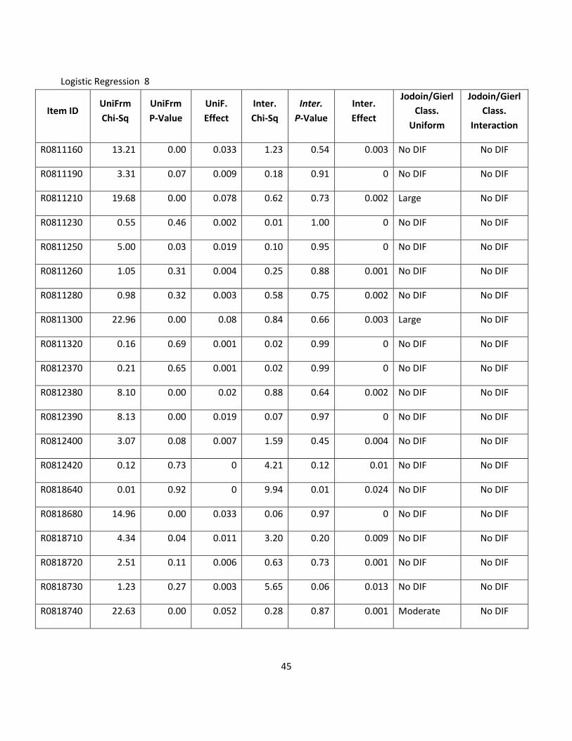
45
Logistic Regression 8
Item ID UniFrm
Chi-Sq
UniFrm
P-Value
UniF.
Effect
Inter.
Chi-Sq
Inter.
P-Value
Inter.
Effect
Jodoin/Gierl
Class.
Uniform
Jodoin/Gierl
Class.
Interaction
R0811160 13.21 0.00 0.033 1.23 0.54 0.003 No DIF No DIF
R0811190 3.31 0.07 0.009 0.18 0.91 0 No DIF No DIF
R0811210 19.68 0.00 0.078 0.62 0.73 0.002 Large No DIF
R0811230 0.55 0.46 0.002 0.01 1.00 0 No DIF No DIF
R0811250 5.00 0.03 0.019 0.10 0.95 0 No DIF No DIF
R0811260 1.05 0.31 0.004 0.25 0.88 0.001 No DIF No DIF
R0811280 0.98 0.32 0.003 0.58 0.75 0.002 No DIF No DIF
R0811300 22.96 0.00 0.08 0.84 0.66 0.003 Large No DIF
R0811320 0.16 0.69 0.001 0.02 0.99 0 No DIF No DIF
R0812370 0.21 0.65 0.001 0.02 0.99 0 No DIF No DIF
R0812380 8.10 0.00 0.02 0.88 0.64 0.002 No DIF No DIF
R0812390 8.13 0.00 0.019 0.07 0.97 0 No DIF No DIF
R0812400 3.07 0.08 0.007 1.59 0.45 0.004 No DIF No DIF
R0812420 0.12 0.73 0 4.21 0.12 0.01 No DIF No DIF
R0818640 0.01 0.92 0 9.94 0.01 0.024 No DIF No DIF
R0818680 14.96 0.00 0.033 0.06 0.97 0 No DIF No DIF
R0818710 4.34 0.04 0.011 3.20 0.20 0.009 No DIF No DIF
R0818720 2.51 0.11 0.006 0.63 0.73 0.001 No DIF No DIF
R0818730 1.23 0.27 0.003 5.65 0.06 0.013 No DIF No DIF
R0818740 22.63 0.00 0.052 0.28 0.87 0.001 Moderate No DIF

46
Logistic Regression 9
Item ID UniFrm
Chi-Sq
UniFrm
P-Value
UniF.
Effect
Inter.
Chi-Sq
Inter. P-
Value
Inter.
Effect
Jodoin/Gierl
Class.
Uniform
Jodoin/Gierl
Class.
Interaction
R0818760 3.38 0.07 0.021 0.07 0.97 0 No DIF No DIF
R0818770 7.80 0.01 0.026 0.01 1.00 0 No DIF No DIF
R0818780 0.05 0.84 0.001 0.36 0.84 0.001 No DIF No DIF
R0818800 0.16 0.69 0.001 2.03 0.36 0.007 No DIF No DIF
R0819020 13.70 0.00 0.023 7.90 0.02 0.014 No DIF No DIF
R0819030 0.40 0.53 0.001 0.01 1.00 0 No DIF No DIF
R0819040 0.49 0.48 0.001 0.18 0.91 0.001 No DIF No DIF
R0819060 0.67 0.41 0.002 5.03 0.08 0.011 No DIF No DIF
R0819070 21.20 0.00 0.042 5.12 0.08 0.01 Moderate No DIF