Ordinary Diﬀerential EquationsOrdinary Diﬀerential Equations Swaroop Nandan Bora...

Ordinary Differential Equations

Swaroop Nandan Bora

[email protected]

Department of Mathematics

Indian Institute of Technology Guwahati

Guwahati-781039

Teachers’ Training Camp, IITG, June 30, 2016

Swaroop Nandan Bora [email protected] (Department of MathematicsIndian Institute of Technology GuwahatiGuwahati-781039 )IITG, Differential EquationsTeachers’ Training Camp, IITG, June 30, 2016

/ 41


/ 41

Modelling a situation

We study a model, a sort of idealized world

that contains things we do not see come across in everyday life.

We study straight lines, rectangles, circles, spheres.

NOT a burger or a chair or a hill or a human being.

If one works in a practical area of mathematics

then there will be two conflicting criteria which makes a good model.

On the one hand,

the model should be accurate enough to be useful.

On the other hand,

it should be simple and elegant enough to generate realistic and interesting

mathematical problem.


/ 41

Modelling a situation

It is tempting, as a mathematician,

to attach far more importance to the second criterion:

mathematical interest and elegance

rather to the first:

accuracy .


/ 41

Mathematicians’ Approach

In particular, if mathematicians work on difficult practical problems

they do not do so in isolation from the rest of mathematics.

Rather, they bring to the problems several tools –

mathematical tricks, rules of thumb, theorems known to be useful and so on.

They do not know in advance which of these tools they will use, but they hope

that

after they have thought hard about a problem they will realize what is needed to solve

it.

If they are lucky, they can simply apply their existing expertise straightforwardly.

More often, they will have to adapt it to some extent.


/ 41

Practical Problems: Applicable mathematics

LET’s now move to the practical side of mathematics in various stages.

In doing so, we need to restrict ourselves

since applications are also as vast as the subject itself.


/ 41

Tea/Coffee

Figure : Hot Coffee


/ 41

Tea/Coffee

Figure : Cold Coffee


/ 41

Falling Body

Figure : Falling Body


/ 41

Pendulum

Figure : Motion of a pendulum


/ 41

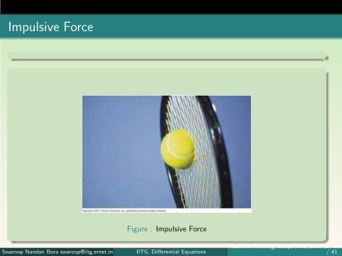
Impulsive Force

Figure : Impulsive Force


/ 41

River

Figure : River flow with current


/ 41

River

Figure : Quiet River flow


/ 41

Sloshing

Figure : Sloshing


/ 41

Building Construction

Figure : Building Construction


/ 41

Flow through porous media

Figure : Aquifer


/ 41

Ocean wave mechanics

Figure : An ocean wave


/ 41

Ocean Engineering

Figure : Rectangular platform in ocean


/ 41

Ocean Engineering

Figure : Offshore Oil drilling platform


/ 41

Figure : An aeroplane in its flight


/ 41

General Information

Many of the general laws of nature – in physics, chemistry, biology and

astronomy –

find their most natural expression in differential equations.

Applications are mainly in the areas of mathematics itself, engineering, economics and

many other fields of applied sciences.

Why is it so??


/ 41

Differential Equations

We know that if y = f(x) is a given function,

then its derivativedy

dxcan be interpreted as the rate of change of y with respect to x.

In many natural processes,

the variables involved and their rates of changes are connected to one another by

means of the basic scientific principles that govern the process.

When this connection is expressed in mathematical symbols, the result is quite often a

differential equation. Let us consider some examples we already know.


/ 41

Example 1

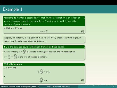
According to Newton’s second law of motion, the acceleration a of a body of

mass m is proportional to the total force F acting on it, with 1/m as the

constant of proportionality,

so that a = F/m or

ma = F. (1)

Suppose, for instance, that a body of mass m falls freely under the action of gravity

alone, then the only force acting on it is mg.

If y is the distance down to the body from some fixed height,

then its velocity v =dy

dtis the rate of change of position and its acceleration

a =dv

dt=

d2y

dt2is the rate of change of velocity.

With this notation,

(22) becomes

md2y

dt2= mg,

or,d2y

dt2= g. (2)


/ 41

Example 1

If we change the situation by assuming that there is an air resistance proportional

to the velocity,

then the total force acting on the body is mg − k(dy/dt).

(22) becomes

md2y

dt2= mg − k

dy

dt. (3)

Equations (??) and (??) are the differential equations that express the essential

attributes of the physical processes under consideration.

They are respectively called undamped and damped motion of the body.


/ 41

Example 2

Newton’s Law of Cooling states that the rate of change of the temperature of an

object is proportional

to the difference between its own temperature and the ambient temperature (i.e. the

temperature of its surroundings).

Newton’s Law makes a statement about an instantaneous rate of change of the

temperature.

When we translate this verbal statement into mathematical symbols,

we arrive at a differential equation.

The solution to this equation will then be a function that tracks the complete record of

the temperature over time.


/ 41

Example 2

If T is the temperature of an object at time t and S is the temperature of its

surroundings,

then this law formulates intodT

dt= −k(T − S), (4)

where k is a constant of proportionality.

If T0 is the initial temperature,

the temperature of the object at any time t is given by

T (t) = S + (T0 − S)e−kt. (5)


/ 41

Example 3

Consider a pendulum of length l

whose bob has a mass m

Then the equation of motion (undamped case) is given by

d2θ

dt2+

g

lsin θ = 0.

Is this the equation we usually know?

Or the equation we know is different from this?

The accepted form is the linearized version

d2θ

dt2+

g

lθ = 0.


/ 41

Boundary and Initial Conditions

Boundary conditions are conditions prescribed on the boundary

Boundary may be boundary with respect to any of the independent variables

Initial conditions are conditions prescribed at one point only

These conditions are in terms of some form of the dependent variable at some

specific value of the independent variable

The main component of this type of problems is what is called Governing Equation


/ 41

Boundary and Initial Conditions (Contd.)

With respect to ODEs

we can have only boundary conditions or only initial conditions, not both for the same

problem

They are called boundary value problems or initial value problems.

However, with respect to PDEs

We can have both boundary conditions and initial conditions for the same problem

This type of problems are called

Initial Boundary Value Problems (IBVP)


/ 41

BVPs and IVPs

A boundary value problem is a differential equation together with a set of additional

constraints, called the boundary conditions.

In other words, a solution to a BVP is a solution to the differential equation which also

satisfies the boundary conditions.

To be useful in applications, a BVP should be well-posed. This means that given the

input to the problem there exists a unique solution, which depends continuously on the

input.

An initial value problem (IVP) consists of a differential equation and a set of

conditions to be satisfied at the initial value of the independent variable (for ODE) or

at that of one of the independent variables (for PDE).


/ 41

BVPs and IVPs

A more mathematical way to picture the difference between a BVP and an IVP is

an IVP has all of the conditions specified at the same value of the independent variable

in the equation (and that value is at the lower value of the boundary of the domain,

thus the term ‘initial’ value), while a BVP has conditions specified at the extremes of

the independent variable.

For example

for a second-order differential equation

if the independent variable is time over the domain [0, 1], an IVP would specify a value

of y(t) and y′(t) at time t = 0, to be precise, the initial conditions will be something

like y(0) = α, y′(0) = β.

On the other hand

a BVP would specify values for y(t) (or its derivatives) at both t = 0 and t = 1, to be

precise, the boundary conditions will be something like y(0) = α1, y(1) = β1 or

y′(0) = α2, y′(1) = β2.


/ 41

IBVPs

If the problem is dependent on both space and time (meaning the governing

equation is a PDE)

then instead of specifying the value of the problem at a given point for all time only,

data could be given at a given time for all space also.

This type of problems is known as initial boundary value problems (IBVP).

Prime examples are the problems

involving the wave equations and the transient heat conduction equations.


/ 41

Types of conditions

The type of boundary conditions that will be considered for a BVP will depend on the

dimension of the object under consideration.

For example

for the heat conduction in a thin rod, the boundaries will be the two end points of the

rod

while

for a thin rectangular plate, the boundary will consist of the four edges that bound the

plate


/ 41

Types of conditions

If the boundary conditions are prescribed in terms of some values of the dependent

variable (solution of the BVP) on the boundary, then these conditions are called

Dirichlet Conditions and the corresponding BVPs are called Dirichlet boundary value

problems

If the boundary conditions are prescribed in terms of some values of the normal

derivatives on the boundary, then these conditions are called

Neumann conditions and the corresponding BVPs are called Neumann boundary value

problems.

Neumann conditions are also known as flux conditions. If there is no flux across the

boundary, then the flux conditions become insulation conditions (for heat conduction

problems).


/ 41

Types of conditions

If the boundary conditions for a specific problem contain both types, then these

conditions are called

mixed or Robin conditions and the corresponding BVPs are called Robin boundary

value problems.

For heat conduction problems, Robin conditions are also known as radiation conditions.

A typical problem in heat conduction may have a combination of Dirichlet,

flux/insulation and radiation boundary conditions.


/ 41

Continuity conditions

Sometimes there may be virtual boundaries.

Say

For a fluid problem, the fluid is of two layers.

Then

at the boundary of the layers, called interface, there exist some conditions

known as

continuity conditions

They usually imply

continuity of pressure and velocity along the boundary


/ 41

Idealizations

Given to us:

a real life problem

Can

we solve the problem exactly with the given conditions?

Perhaps not.

Under this circumstances

we need to idealize the situation, that is, we want to ignore some of the given

situations/properties in order to obtain a feasible solution.

What do we do?


/ 41

Idealizations

Idealization can take place in three ways

Property

Governing Equation

Boundary Conditions

We need to idealize the situation, that is, we want to ignore some of the given

situations/properties in order to obtain a feasible solution.


/ 41

Moving ahead

Recall Newton’s Second Law of Motion

F = ma

In terms of differential equation, it is

d2y

dt2= g

and the solution can be obtained as

y =gt2

2+ c1t+ c2

Given two initial conditions

the arbitrary constants can be eliminated


/ 41

Moving ahead

Does the equation represent the real situation?

Perhaps not. What was ignored??

–The air resistance the particle encounters while falling down

If air resistance is taken into account,

md2y

dt2= mg − k

dy

dt

A new term is appended due to the air resistance

The former equation is an idealized version of the latter one.


/ 41

Moving ahead

Now consider the pendulum equation

What was ignored??

–The air resistance the bob encounters while moving from one end to the other

Now what we will have a

damped version of the equation.


/ 41

Remarks

There are many functions/polynomials

which are solutions of some specific ODEs.

They are called special functions, such as

Bessel function, Legendre polynomial, Hermite polynomial, Laguerre polynomial etc.

More interestingly, they

are part of Mathematical Physics rather than only of Mathematics.


/ 41

Ordinary Diﬀerential EquationsOrdinary Diﬀerential Equations Swaroop Nandan Bora...

Documents

Transcript of Ordinary Diﬀerential EquationsOrdinary Diﬀerential Equations Swaroop Nandan Bora...