Ordinary Differential Equationshomepages.math.uic.edu/~jan/mcs507f12/solvingodes.pdf · Jan...

Ordinary Differential Equations

1 An Oscillating Pendulumapplying the forward Euler methodusing odeint in odepack of scipy.integrate

2 Celestial Mechanicssimulating the n-body problemusing odeint in odepack of scipy.integrate

3 The Tractrix Problemsetting up the differential equationsusing odeint in odepack of scipy.integrate

MCS 507 Lecture 24Mathematical, Statistical and Scientific Software

Jan Verschelde, 22 October 2012

Scientific Software (MCS 507) Ordinary Differential Equations 22 October 2012 1 / 38

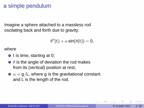
a simple pendulum

Imagine a sphere attached to a massless rodoscilating back and forth due to gravity:

θ′′(t) + α sin(θ(t)) = 0,

where

t is time, starting at 0;

θ is the angle of deviation the rod makesfrom its (vertical) position at rest;

α = g/L, where g is the gravitational constantand L is the length of the rod.


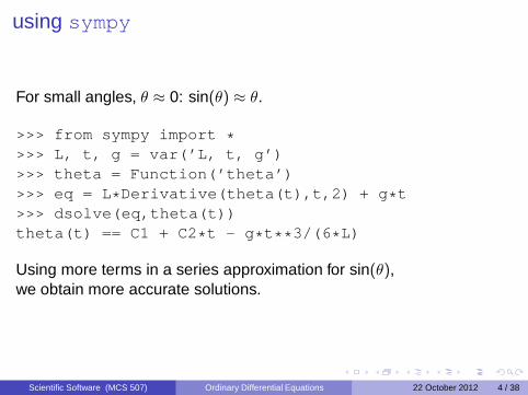
using sympy

For small angles, θ ≈ 0: sin(θ) ≈ θ.

>>> from sympy import *>>> L, t, g = var(’L, t, g’)>>> theta = Function(’theta’)>>> eq = L*Derivative(theta(t),t,2) + g*t>>> dsolve(eq,theta(t))theta(t) == C1 + C2*t - g*t**3/(6*L)

Using more terms in a series approximation for sin(θ),we obtain more accurate solutions.


first order equations

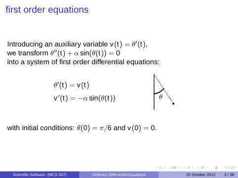
Introducing an auxiliary variable v(t) = θ′(t),we transform θ′′(t) + α sin(θ(t)) = 0into a system of first order differential equations:

JJJJJ

θr

θ′(t) = v(t)

v ′(t) = −α sin(θ(t))

with initial conditions: θ(0) = π/6 and v(0) = 0.


forward Euler method

We use the definition θ′(t) = limh→0

θ(t + h) − θ(t)h

to discretize the time domain with step size ∆t .

At t = tk , we approximate θ(tk ) ≈ θk andθ(tk+1) ≈ θk+1 for and tk+1 = tk + ∆t .

So θ′(t) = v(t) is approximated byθk+1 − θk

∆t= vk .

Then we compute θk+1 = θk + ∆tvk .

Similarly, v ′(t) = −α sin(θ(t))is approximated by vk+1 = vk − α∆t sin(θk ).


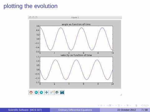
plotting the evolution


programming the Euler method

import scipy as spimport matplotlib.pyplot as plt

def pendulum(T,n,theta0,v0,alpha):"""Return the motion (theta, v, t) ofa pendulum, governed by the ODE:theta’’(t) + alpha*sin(theta(t)) = 0,where the parameters are

T : time t ranges from 0 to T,n : the number of time steps,theta0 : angle at t = 0,v0 : velocity at t = 0,alpha : value for the parameter.

"""


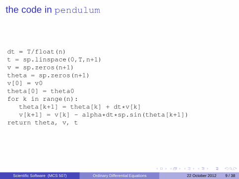
the code in pendulum

dt = T/float(n)t = sp.linspace(0,T,n+1)v = sp.zeros(n+1)theta = sp.zeros(n+1)v[0] = v0theta[0] = theta0for k in range(n):

theta[k+1] = theta[k] + dt*v[k]v[k+1] = v[k] - alpha*dt*sp.sin(theta[k+1])

return theta, v, t


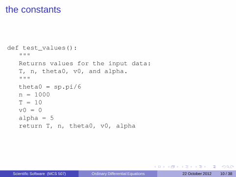
the constants

def test_values():"""Returns values for the input data:T, n, theta0, v0, and alpha."""theta0 = sp.pi/6n = 1000T = 10v0 = 0alpha = 5return T, n, theta0, v0, alpha


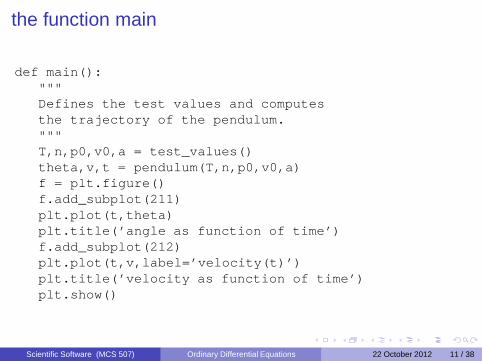
the function main

def main():"""Defines the test values and computesthe trajectory of the pendulum."""T,n,p0,v0,a = test_values()theta,v,t = pendulum(T,n,p0,v0,a)f = plt.figure()f.add_subplot(211)plt.plot(t,theta)plt.title(’angle as function of time’)f.add_subplot(212)plt.plot(t,v,label=’velocity(t)’)plt.title(’velocity as function of time’)plt.show()


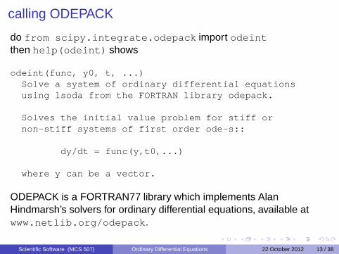
calling ODEPACK

do from scipy.integrate.odepack import odeintthen help(odeint) shows

odeint(func, y0, t, ...)Solve a system of ordinary differential equationsusing lsoda from the FORTRAN library odepack.

Solves the initial value problem for stiff ornon-stiff systems of first order ode-s::

dy/dt = func(y,t0,...)

where y can be a vector.

ODEPACK is a FORTRAN77 library which implements AlanHindmarsh’s solvers for ordinary differential equations, available atwww.netlib.org/odepack.


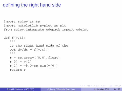
defining the right hand side

import scipy as spimport matplotlib.pyplot as pltfrom scipy.integrate.odepack import odeint

def f(y,t):"""Is the right hand side of theODE dy/dt = f(y,t)."""r = sp.array([0,0],float)r[0] = y[1]r[1] = -5.0*sp.sin(y[0])return r


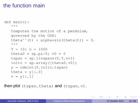
the function main

def main():"""Computes the motion of a pendulum,governed by the ODE:theta’’(t) + alpha*sin(theta(t)) = 0,"""T = 10; n = 1000theta0 = sp.pi/6; v0 = 0tspan = sp.linspace(0,T,n+1)initc = sp.array([theta0,v0])y = odeint(f,initc,tspan)theta = y[:,0]v = y[:,1]

then plot (tspan,theta) and (tspan,v).


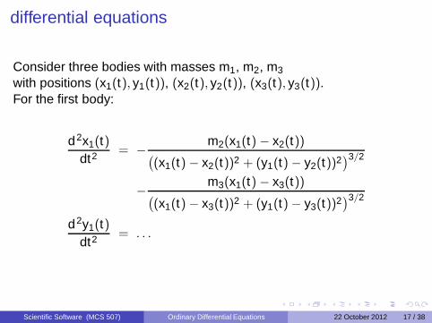
differential equations

Consider three bodies with masses m1, m2, m3

with positions (x1(t), y1(t)), (x2(t), y2(t)), (x3(t), y3(t)).For the first body:

d2x1(t)dt2 = −

m2(x1(t) − x2(t))(

(x1(t) − x2(t))2 + (y1(t) − y2(t))2)3/2

−m3(x1(t) − x3(t))

(

(x1(t) − x3(t))2 + (y1(t) − y3(t))2)3/2

d2y1(t)dt2 = . . .


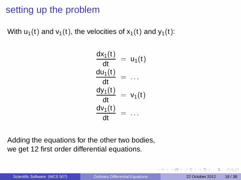
setting up the problem

With u1(t) and v1(t), the velocities of x1(t) and y1(t):

dx1(t)dt

= u1(t)

du1(t)dt

= . . .

dy1(t)dt

= v1(t)

dv1(t)dt

= . . .

Adding the equations for the other two bodies,we get 12 first order differential equations.


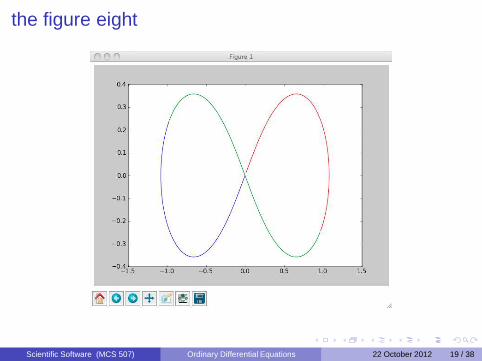
the figure eight


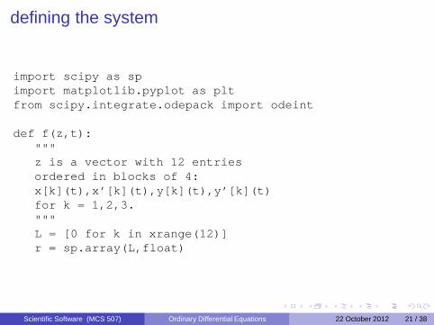
defining the system

import scipy as spimport matplotlib.pyplot as pltfrom scipy.integrate.odepack import odeint

def f(z,t):"""z is a vector with 12 entriesordered in blocks of 4:x[k](t),x’[k](t),y[k](t),y’[k](t)for k = 1,2,3."""L = [0 for k in xrange(12)]r = sp.array(L,float)


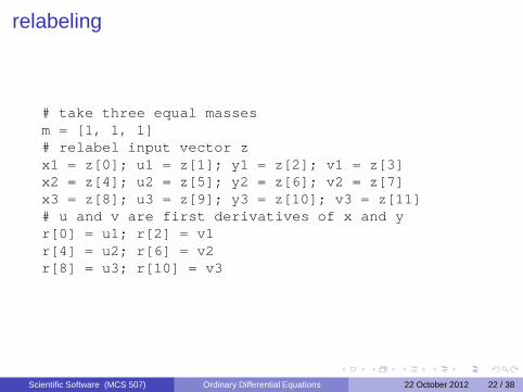
relabeling

# take three equal massesm = [1, 1, 1]# relabel input vector zx1 = z[0]; u1 = z[1]; y1 = z[2]; v1 = z[3]x2 = z[4]; u2 = z[5]; y2 = z[6]; v2 = z[7]x3 = z[8]; u3 = z[9]; y3 = z[10]; v3 = z[11]# u and v are first derivatives of x and yr[0] = u1; r[2] = v1r[4] = u2; r[6] = v2r[8] = u3; r[10] = v3


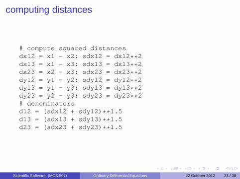
computing distances

# compute squared distancesdx12 = x1 - x2; sdx12 = dx12**2dx13 = x1 - x3; sdx13 = dx13**2dx23 = x2 - x3; sdx23 = dx23**2dy12 = y1 - y2; sdy12 = dy12**2dy13 = y1 - y3; sdy13 = dy13**2dy23 = y2 - y3; sdy23 = dy23**2# denominatorsd12 = (sdx12 + sdy12)**1.5d13 = (sdx13 + sdy13)**1.5d23 = (sdx23 + sdy23)**1.5


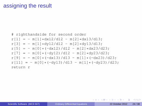
assigning the result

# righthandside for second orderr[1] = - m[1]*dx12/d12 - m[2]*dx13/d13;r[3] = - m[1]*dy12/d12 - m[2]*dy13/d13;r[5] = - m[0]*(-dx12)/d12 - m[2]*dx23/d23;r[7] = - m[0]*(-dy12)/d12 - m[2]*dy23/d23;r[9] = - m[0]*(-dx13)/d13 - m[1]*(-dx23)/d23;r[11] = - m[0]*(-dy13)/d13 - m[1]*(-dy23)/d23;return r


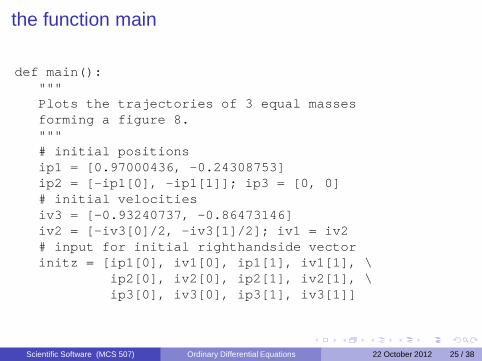
the function main

def main():"""Plots the trajectories of 3 equal massesforming a figure 8."""# initial positionsip1 = [0.97000436, -0.24308753]ip2 = [-ip1[0], -ip1[1]]; ip3 = [0, 0]# initial velocitiesiv3 = [-0.93240737, -0.86473146]iv2 = [-iv3[0]/2, -iv3[1]/2]; iv1 = iv2# input for initial righthandside vectorinitz = [ip1[0], iv1[0], ip1[1], iv1[1], \

ip2[0], iv2[0], ip2[1], iv2[1], \ip3[0], iv3[0], ip3[1], iv3[1]]


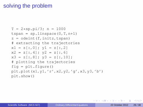
solving the problem

T = 2*sp.pi/3; n = 1000tspan = sp.linspace(0,T,n+1)z = odeint(f,initz,tspan)# extracting the trajectoriesx1 = z[:,0]; y1 = z[:,2]x2 = z[:,4]; y2 = z[:,6]x3 = z[:,8]; y3 = z[:,10];# plotting the trajectoriesfig = plt.figure()plt.plot(x1,y1,’r’,x2,y2,’g’,x3,y3,’b’)plt.show()


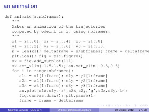
an animation

def animate(z,nbframes):"""Makes an animation of the trajectoriescomputed by odeint in z, using nbframes."""x1 = z[:,0]; x2 = z[:,4]; x3 = z[:,8]y1 = z[:,2]; y2 = z[:,6]; y3 = z[:,10]n = len(x1); deltaframe = n/nbframes; frame = deltaframeplt.ion(); fig = plt.figure()ax = fig.add_subplot(111)ax.set_xlim(-1.5,1.5); ax.set_ylim(-0.5,0.5)for i in range(nbframes):

s1x = x1[1:frame]; s1y = y1[1:frame]s2x = x2[1:frame]; s2y = y2[1:frame]s3x = x3[1:frame]; s3y = y3[1:frame]ax.plot(s1x,s1y,’r’,s2x,s2y,’g’,s3x,s3y,’b’)fig.canvas.draw(); plt.pause(1)frame = frame + deltaframe


the tractrix problem

A tractor is connected to a trailer bya rigid bar of unit length.

The tractor moves in a circle.

The path of the trailer is the solution ofa system of ordinary differential equations.

Generalization: trailer is predator, tractor is prey.


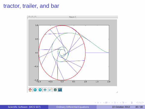
tractor, trailer, and bar


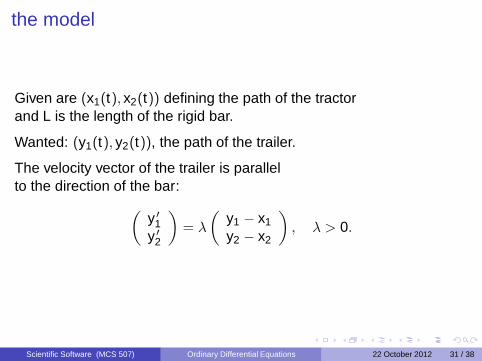
the model

Given are (x1(t), x2(t)) defining the path of the tractorand L is the length of the rigid bar.

Wanted: (y1(t), y2(t)), the path of the trailer.

The velocity vector of the trailer is parallelto the direction of the bar:

(

y ′

1y ′

2

)

= λ

(

y1 − x1

y2 − x2

)

, λ > 0.


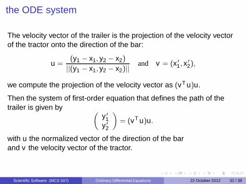
the ODE system

The velocity vector of the trailer is the projection of the velocity vectorof the tractor onto the direction of the bar:

u =(y1 − x1, y2 − x2)

||(y1 − x1, y2 − x2)||and v = (x ′

1, x ′

2),

we compute the projection of the velocity vector as (vT u)u.

Then the system of first-order equation that defines the path of thetrailer is given by

(

y ′

1y ′

2

)

= (vT u)u.

with u the normalized vector of the direction of the barand v the velocity vector of the tractor.


the tractor

import scipy as spimport numpy as npimport matplotlib.pyplot as pltfrom scipy.integrate.odepack import odeint

def tractor(t):"""Returns the position (x,y)and velocity vector (u,v)for the tractor at time t."""x = sp.cos(t); y = sp.sin(t)u = -sp.sin(t); v = sp.cos(t)return x,y,u,v


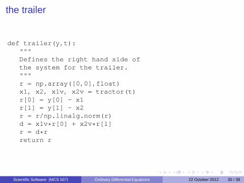
the trailer

def trailer(y,t):"""Defines the right hand side ofthe system for the trailer."""r = np.array([0,0],float)x1, x2, x1v, x2v = tractor(t)r[0] = y[0] - x1r[1] = y[1] - x2r = r/np.linalg.norm(r)d = x1v*r[0] + x2v*r[1]r = d*rreturn r


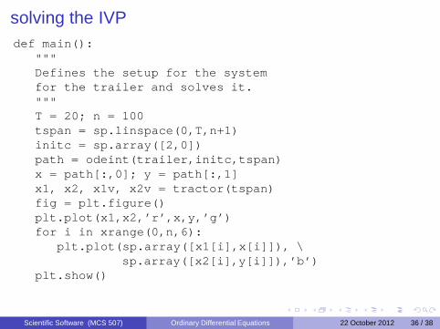
solving the IVPdef main():

"""Defines the setup for the systemfor the trailer and solves it."""T = 20; n = 100tspan = sp.linspace(0,T,n+1)initc = sp.array([2,0])path = odeint(trailer,initc,tspan)x = path[:,0]; y = path[:,1]x1, x2, x1v, x2v = tractor(tspan)fig = plt.figure()plt.plot(x1,x2,’r’,x,y,’g’)for i in xrange(0,n,6):

plt.plot(sp.array([x1[i],x[i]]), \sp.array([x2[i],y[i]]),’b’)

plt.show()


Summary + Exercises

Appendices C, D, and E of the book are on differential equations.SciPy.integrate exports odeint() of odepack.

A.C. Hindmarsh: ODEPACK, A Systematized Collection of ODESolvers. In IMACS Transactions on Scientific Computation, Volume 1,pages 55-64, 1983, edited by R.S. Stepleman.

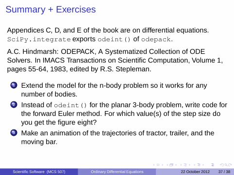
1 Extend the model for the n-body problem so it works for anynumber of bodies.

2 Instead of odeint() for the planar 3-body problem, write code forthe forward Euler method. For which value(s) of the step size doyou get the figure eight?

3 Make an animation of the trajectories of tractor, trailer, and themoving bar.


more exercises

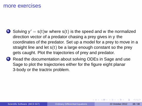
4 Solving y ′ = s(t)w where s(t) is the speed and w the normalizeddirection vector of a predator chasing a prey gives in y thecoordinates of the predator. Set up a model for a prey to move in astraight line and let s(t) be a large enough constant so the preygets caught. Plot the trajectories of prey and predator.

5 Read the documentation about solving ODEs in Sage and useSage to plot the trajectories either for the figure eight planar3-body or the tractrix problem.


Ordinary Differential Equationshomepages.math.uic.edu/~jan/mcs507f12/solvingodes.pdf · Jan...

Documents

Transcript of Ordinary Differential Equationshomepages.math.uic.edu/~jan/mcs507f12/solvingodes.pdf · Jan...