1

Ordinary differential equationsaccording to the text book with this title by V.I. Arnol’d.

Introductionary lectures held at Leipzig University during the summer semester 2011by B. HerzogFr. 7.30 - 9.00, Ph. 2-18 (exercises)Fr. 9.15 - 10.45, Ph. 2-18 (lectures)

Exercises and lectures from July 15, 2011 are moved to

Fr. July 22, 15.00-18.00, Math Institute, Felix-Klein-Hörsaal, Johannisgasse.Mo. July 25, 15.00-18.00, Math Institute, Felix-Klein-Hörsaal, Johannisgasse.

Writen examination:July 26, 8.00-11.00, Room 1-22, Mathematical Institute, JohannisgasseRepetition:September 26, 8.00-11.00, Room S 114, Augustusplaz

Conditions• There will be a written test at the end of the semester.• To enter this test you will have to solve problems every week.• Each week you will usually have to deal with three problems, whose solutions you

will have to return in written form at the beginning of the exicises at Fridaymoring.

• For each solution you can achieve up to three points. For the right to enter thewritten examination you need 50% of the maximum number of points.

Notation∂X boundary of the set X (in some topological space), see 2.2.2.∂∂xi

, ∂∂x ,∂∂t derivatives in the directions of, respectively, the xi - , x-, and t- axes, which

are identified with the standard unit vectors in the direction of these axes,see 1.4.2.

dxdt (t0) the tangent vektor of the curve x: I H M, t ! x(t), at the point x(t0), see

Example 4 of 1.4.3.∂f∂x (p) the Jacobian matrix of a map f: U H V between open sets U, V in

euclidian space at the point p P U, see Appendix.dpϕ differential of a map ϕ: M H M’ at the point pPM, see 1.4.3, (which is

a linear map dpϕ: Tp(M) H Tϕ(p)(M’), in appropriately chosen

coordinates it is multiplication by the Jacobian matrix of ϕ, see 1.4.3Example 2).

dϕ differential form of a map ϕ: M H M’, see Remark (iii) of 1.4.7,(which is the map ϕ: TM H TM’ whose restriction to Tp(M) is dpϕ

for every pPM).Aut(M) transformation group of the set M, see 1.2.2.OM,p local ring of the manifold M at the point p, see 1.4.1.

2

TM tangent bundle of a manifold, see 1.4.6.Tp(M) tangent space of the manifold M at the point pPM, see 1.4.2.

Γf graph of the map f: A H B, i.e., Γf := {(a,f(a)) | aPA}.

S(I, A) The space of solution I H Rn of the linear differential equation dxdt =

A(t):x, see 2.2.1. B.

1. Basic notions

1.1. A first definitionAn ordinary differential equation (ODE) is an equation depending upon a function, say

x = x(t),

together with certain derivatives of this function and the variable t. In other words, anordinary differential equation is something like this:

f(x, dxdt , d

2xdt2

, ... , dnx

dtn , t) = 0. (1)

More precisely, such an equation is called n-th order ordinary differential equation.

The topic of the theory is to find solutions (one, as many as possible or all) of such anequation, i.e. all functions x such that this equation becomes an identity.

Moreover, one wants to find qualitative properties of the solutions.

Remarks(i) We do not assume, that the values of the function x are real or complex numbers.

They may be contained in any set, where differention is possible. Typically,x(t) P Rn.

Likewise we allow f to be a vector valued function,f(y0, y1, ... , yn) P Rm.

This way there will be not really a difference between one single differentialequation and a system of such equations.

(ii) On the other hand, the variable t is always assumed to vary in an open subset ofthe real axis,

t P U é R, U open.Remember, open means, for every value t in U there is an open intervall around t,which is completely contained in U,

t P U " t P ( t - ε , t + ε ) é U for some ε > 0.(iii) Consider a massive particle (of mass equal to m) moving with the time t in 3-space,

sayx(t) P R3,

such thatd2x(t)

dt2 - g/m = 0.

This ordinary differential equation is probably the first one has to solve in classicalmechanics.

3

(vi) A considerable part of mathematics and physics is related to differential equations,for example

∂2x∂u2 + ∂

2x∂v2 + ∂

2x∂w2 = 0 , x(u, v, w) PR, (Laplace-Gleichung) (2)

or∂2x∂u2 + ∂

2x∂v2 + ∂

2x∂w2 - ∂

2x∂t2

= 0 , x (u, v, w) PR, (Wellen-Gleichung) (3)

or∂f(u,v)∂u + i:∂f(u,v)

∂v = 0, f(u,v) PC (Cauchy-Riemann equations) (4)

Other examples arethe Hamiltopn equations in classical mechanics,the Maxwell equations in electrodynamics,the Schrödinger equation in Quantum mechanicsor various Yang-Mills equantions in Quantum field theory.

All these equations are not ordinary differential equations, since they containpartial derivatives with respect to different variables. They are partial differentialequations (PDE’s).

(vii) There are essential differences between ordinary and partial differential equations:

• The theory of ODE’s is much easier than any theory of PDE’s. If you want tounderstand partial differential equations you need a good knowledge of thebehavior of the ordinary ones.

• One can even say there is a well understood theory about the behavior of allODE’s, while there is no common theory of PDE’s. Two different PDE’s usuallyrequire different theories. Even the questions one has to ask for are usuallydifferent for different PDE’s.

• The theory of the equations of type (2) is called Potential theory in the real case orHodge theory in the complex projective case.

• Those of type (3) lead to (classical) wave theory.• Those of type (4) result in complex analysis.• The theory of the (finitie dimensional) Hamilton equations is called simplectic

geometry (or classical mechanics).• etc.

(vii) Our topic, the ordinary differential equations, is much easier.

Convention: If not stated otherwise, we will always assume that the functions solvingour equations are sufficiently often continuously differentiables.

Problem 2:(viii) Note that every systems n-th order ODE’s is equivalent to system of first order

ODE’s.

Two systems ODE’s are called equivalent in case they have (essentially) the samesolutions (i.e. the solutions of one system can be directly seen from the solutionsof the other).

Equation (1) can be written as follows.

f(x0, x1 , x2 , ... , xn, t) = 0.x1 = dx0/dt

4

x2 = dx1/dt...xn = dxn-1/dt

We introduce a new notation:X := (x0, x1 , x2 , ... , xn), Y = (y0, y1 , y2 , ... , yn)F(X, Y,t) := ( f(x0, x1 , x2 , ... , xn,t), x1 - y0 , x2 - y1 , ... , xn - yn-1).

Then the above system readsF(X, dX

dt ,t) = 0.This way we see that an n-th order ODE is equivalent to an first oder ODE.

To start with, we will give a quite different look at the theory of ordinary differentialequations.

1.2 Phase spaces and phase flows

1.2.1 Finite dimensional deterministic processesThe theory of ordinary differential equations deals with deterministic, finite dimensionaland differential processes evolving in time.

Finite dimensional means, the state of such a process is given by a point in a finitedimensional space (i.e. by a finite number of parameters). This space, consisting of allpossible states, is called phase space.

Deterministic means, that all future and all past states are uniquely determined by thecurrent state.

Formally, if M denotes the phase space, there is a map g: R;M H M, (t, x) ! gtx,

such that gtx is the state of the process at time t whose state at time 0 is x.

In other word, given the state x at time 0, the state gtx at time t of this process is uniquelydetermined.

The map g is called the phase flow of the process.

The process is called differentiable, if M ist a space where differentiaton is defined (adifferentiable manifold) and the map g is differentiable.

Remarks(i) Let x be the state of the process at time 0. Than its state at time t is gtx.

Similarly, if y is the state at time s, its state at time s+t is gsy. Substituting gtx fory we obtain

gs+tx = gsgtx for arbitrary x P M, s, t PR. (1)

time state0 xt gtx

5

s+t gsgty

Moreover, by the very definition of the phase flow,

g0x = x for each x P M. (2)

The identities (1) and (2) are the most important properties of the phase flow.

(ii) For each t PR the phase flow defines a mapgt: M H M, x ! gtx.

Thus we have a family of maps{gt}tPR

Note that the composition of any two maps in this family is again a map in thisfamily:

gsgt = gs+t.The family {gt}tPR is called the one-parameter group of transformations

associated with the phase flow g.

Problem 1: Prove that each map of the family {gt}tPR is bijective and that these

maps form a commutative group.

(iii) The notion of phase space is the most important notion in our context. Often theintroduction of the phase space of a problem is already the solution of theproblem.

ExampleConsider two cities connected by two none-intersecting roads, say city A and city B.

A B

About these two roads the following fact is known:

Assume that there are two cars in city A, which are connected by a cord of length < 2:l.Then we know that it is possible for these cars to travel to city B on different roadswithout breaking the cord.

Question:Assume that there are two circular wagons (moving discs) of radius l, one in city A andone in city B. Is it possible to move these two wagons simultaneously to the other citywithout touching each other ?

Intuitively one would expect that this is impossible. But how to prove this ?

6

It turns out that the solution is to form the phase space describing the situation. Themovement of each car or wagon it given by the single parameter, namely the distance ithas moved from its city on its road.

Denote the distance on the first road by x and the distance on the second by y. We mayassume that both roads have the same length 1 (we may use for each road its own unit tomeasure the distances). Thus both parameters vary between 0 and 1,

0 ≤ x ≤ 1, 0 ≤ y ≤ 1.Therefore, the positions of two bodies on the two roads is given by a point in the square

M := { (x, y) P R2 | 0 ≤ x ≤ 1, 0 ≤ y ≤ 1 }Assume that both roads start in city A and end in city B, i.e. the coordinate 0 describes inboth roads the starting point in city A and the coordinate 1 describes city B.

The movement from A to B of the two cars is given by a curve γ from (0,0) to (1,1), sinceboth start in the same city A and end in the same city B.

Similarly, the movement of the two wagons is given by a curve δ from (1,0) to (0,1). Thesituation tells us that the two curves must intersect.1

γ

δ

M

Let (x,y) be a point of intersection. This point describes a situation, where the two carsare in the same position like the two wagons. But the distance of the two cars is beassumption less than 2:l, while the two wagons should be at a distance greater than 2:l,which is impossible.

There are no ODE’s involved in the above problem. But we see that the pureconstruction of the phase space already solves a not quite trivial problem !

1.2.2 One-parameter groups of transformationsLet M be a set. A transformation (or automorphism) of M ist simply a bijektive map

M H M.The transformations of M form a group, denoted

1 Each curve divides the square in two components, and the other curve connects points of differentcomponents.

7

Aut(M),

whose group law is the usual composition of maps. A one-parameter group oftransformations (or automorphisms) is by definition a group homomorphisms

h:R H Aut(M), t ! htfrom the additive group of real numbers to the transformation group Aut(M).Equivalently, a one-paramter group is given by a map

R;M H M, (t, x) ! ht(x),such that1. h0(x) = x for every x P M2. hs(ht(x)) = hs+t(x) for every x P M and arbitrary s,t P R.Remarks(i) The one-parameter group of a phase flow is obviously a one-parameter group in

the sense just defined.(ii) In case M is a (finite dimensional) differentiable manifold, and h is a differentiable

map, than h is nothing else but a phase flow.

1.2.3 Phase curves and fixed points of the phase flowLet M be a phase space with phase flow

g: R;M H M, (t, x) ! gt(x).Then for each point x the map

R H M, t ! gt(x),is called the motion of the point x under the effect of the phase flow g. The image of thismap is called the phase curve through x or the trajectory through x.In case the phase curve through x consists of one single point, i.e.,

gt(x) = g0(x) = x for every t PR,

the point x is called equilibrium or fixed point of the phase flow.

The space R;M is also called extended phase space of the given flow. An integral curveof the flow is by definition the graph of a motion of the flow, i.e. a set in the extendedphase space of the type

{ (t, gt(x) | t P R}

RemarkThe line R;{x} is an integral curve if and only if the point x is a fixed point of theflow.

The R;{x} is an integral curve if and only if there is some point x’PM such thatR;{x} = { (t, gt(x’) | t P R},

8

i..e.,gt(x’) = x for every t PR.

For t = 0 this latter condition gives x’ = g0x’ = x. Thus:

R;{x} is an integral curve $ gt(x) = x for every t PR.

The condition on the right hand side means that x is a fixed point of the flow.

Problem 2Prove that there is precisely one integral curce through each point of the extended phasespace.Problem 3Prove that for every s PR, the following translation of the extended phase space mapsintegral curves into integral curves.

hs: R;M H R;M, (t, x) ! (t + s, x).

1.2.4 Phase flows and direction fields in the planeLet g: R;M H M a phase flow with M = R. Through every point

(t0, x0) P R2

of the extented phase space goes presicely one integral curve

C(t0, x0) = {(t, gtg-t0x0) | t P R}.

LetT(t0, x0)

denote the tangent to this curve at the given point (t0, x0). This way we get a map

T: R2 H {lines in R2}which associates with each point in R2 a lin going through this point. Such a map iscalled direction field.

(t , x)

t

x

C (t,x)

1

v(t,x)

T(t,x)

9

Problem: Is it possible to recalculate the integral curves of the flow from this directionfield ?

Generalization of the problem: forget that the direction field comes from a flow.

A curve is called integral curve of a direction field if the tangent line at any point of thecurve is equal to the line of the direction field at that point.

Generalized problem: how to find integral curves of direction fields.

More precisely, letv(t, x)

denote the slope of the direction field line associated with the point (t,x). The problem isto recalculate the integral curves from the function

v: R2 H RÕ{§}.Equivalently, solve the differential equation

dxdt = v(t, x).

A trivial caseAssume the the following additional conditions are satisfied1) There is no direction in the field parallel to the x-axis.2) Translations in the direction of the x-axis map the lines of the direction field into

lines of that field.

•The first condition means, the the values of v are always finite and the integralcurves are graphs of functions, say

x = x(t).• The second condition means,

v = v(t)does not depent upon x.

• The graph of the function x = x(t) is an integral curve, if and only ifdxdt = v(t).

Integration yields

⌡⌠t0

t dxdt dt = ⌡⌠

t0

t v(t) dt

hence

x(t) = x(t0) + ⌡⌠t0

t v(t) dt.

A less trivial case: dxdt = v(x).

This is not the type of equation corresponding to the above trivial case. But it asks forthe integral curves of a given direction field.

But there is another problem with the same solution: look for a function t = t(x), suchthat the graph is an integral curve of the given direction field. The differential equationfor this problem,

dtdx = 1

v(x) ,can be solved:

10

t(x) = t(x0) + ⌡⌠x0

x dxv(x)

Condition: v(x) should be continuos and none-zero.Example: The equation of normal reproduction

dxdt = x.

(Remove the t-axis x = 0 from R2).Solution:

t = t0 + ⌡⌠x0

x dx

x

= t0 + [ln |x|]xx0

= t0 + (ln |x| - ln |x0|)= t0 + ln |x/x0|

et-t0 = |x/x0|

x = x0: et-t0

The graph of this curve is the ingral curve through the point (t0, x0).The general (phase flow) case:As we know, translations in the diretion of the t-axis map integral curves of phase flowsinto integral curves. This means that the function v(t,x) does not depend upton t. Thusthe above solved problem is already the general case.Remarks(i) Liouville has proved that the equation

dxdt = x2 - t.

cannot be solved just by integration.(ii) A slight generalization of the above example,

dxdt = k:x

decribes population growth2 for k > 0 and radioactive decay for k < 0 (or air density)3.Calculations like above give:

x = x0: ek(t-t0)

The most remarkable property of this function is, that there is a constant time periodafter which the absolute value of x doubles:

T = k-1: ln(2)( T is negative if so is k, and |T| is called half life in this case).(iii) The above equation of normal reproduction describes population growth only fora restricted time period. At some point the population might become too large, so that theway of development changes due to food problems. One way to get a model for thisphenomen is to assume that the constant k above depends upon the size of thepopulation,

k = k(x).In the simplest type of model one assumes the k is a linear function of x, say 2 Population growth is proportional to the number of individuals.3 Air density is half as large at Mt. Elbrus in abour 5,6 km height compared with the density at sealevel.

11

k = a - bx.An easy transformation leads to the differential equation

dxdt = (1 - x)x.

This equation has an instable4 equilibrium atx = 0.

and a stable5 equilibrium atx = 1

All integral curves in the upper half plane are asymptotic to the curve x = 0.

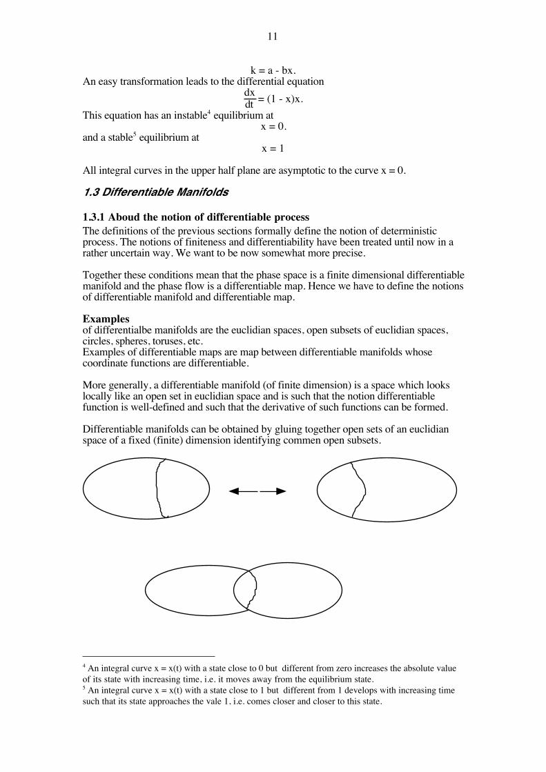
1.3 Differentiable Manifolds

1.3.1 Aboud the notion of differentiable processThe definitions of the previous sections formally define the notion of deterministicprocess. The notions of finiteness and differentiability have been treated until now in arather uncertain way. We want to be now somewhat more precise.

Together these conditions mean that the phase space is a finite dimensional differentiablemanifold and the phase flow is a differentiable map. Hence we have to define the notionsof differentiable manifold and differentiable map.

Examplesof differentialbe manifolds are the euclidian spaces, open subsets of euclidian spaces,circles, spheres, toruses, etc.Examples of differentiable maps are map between differentiable manifolds whosecoordinate functions are differentiable.

More generally, a differentiable manifold (of finite dimension) is a space which lookslocally like an open set in euclidian space and is such that the notion differentiablefunction is well-defined and such that the derivative of such functions can be formed.

Differentiable manifolds can be obtained by gluing together open sets of an euclidianspace of a fixed (finite) dimension identifying commen open subsets.

4 An integral curve x = x(t) with a state close to 0 but different from zero increases the absolute valueof its state with increasing time, i.e. it moves away from the equilibrium state.5 An integral curve x = x(t) with a state close to 1 but different from 1 develops with increasing timesuch that its state approaches the vale 1, i.e. comes closer and closer to this state.

12

The identification has to be done in such a way that the notions of differentiability onboth piecs coicide, i.e. one has to use bijective maps which are differentiable in bothdirections.

To give a more formal definition, we have first to introduce the notion of topologicalspace.

1.3.2 Topological spacesA topological space is a set X together with a family T(X) of subsets of X, called opensets of X, such that the following conditions are satisfied.

(i) The empty set and the whole space are open sets of X, i.e.,$ P T(X) and X P T(X).

(ii) The intersection of any two open sets is open, i.e.,U, V P T(X) " U,V P T(X).

(iii) The union of any family of open sets is open, i.e.,Ui P T(X) for every i P I " ÕiPI Ui P T(X).

In this situation, the family T(X) is called the topology of X. An open set UPT(X)containing a given point x P X is also called (open) neightbourhood of x.

A topological space X is called Hausdorff space , if there exist, for any two givendifferent points x, y P X , open subsets U, V é X such that

x P U, y P V and U,V = $.A map f: X H X’ between topological spaces X and X’ is called continuous, if forevery open set U’PT(X’) the set

f-1(U’) := {xPX | f(x) P U’}is an open set of X.

The map f: X H X’ is called a homeomorphism, if it is bijective and both f and f-1 arecontinuous. In this case X and X’ are called homeomorph. As topological spaces theyare consindered as essentially equal.

ExampleFor every set X the family

T(X) := {U | U é X}of all subsets defines on X the structure of a topological space. This topology T(X) iscalled discrete topology of X. The topological space whose topology is the discrete oneis called discrete topological space. A discrete topological space is always a Hausdorffspace.ExampleFor every set X the family

T(X) = {$, X}defines a topology on X. If X is equipped with this topology and has at least two points,it is never a Hausdorff space (each point is in every neighbourhood.ExampleFor every two points x = (x1,...,xn) and y = (y1,...,yn) in Rn write

13

d(x, y) := (x1-y1)2+...+(xn-yn)2

for the distance between x and y und denote byUε(x) := {y P Rn | d(y, x) < ε}

the ε−neightbourhood of all points of distance less than ε from x. A subsetU é Rn

is called open, if there is, for every x P U there is some positive real number ε such thatUε(x) is completely containted in U,

x P U " Uε(x) é U for some positive real ε.

The set T(Rn) of all open sets of Rn as just defined is called the euclidian topology ofRn. One can easily prove that a map

f: Rn H Rm,where both spaces are equipped with the euklidian topology, is continuous in the abovedefined sense if and only if it safisfies the conditions of the δ−ε-criterion.

A examples of an open set in R2 is the open disc of radius r around the origin o :=(0,0),

Ur(o) is open in R2.The closed disc (including the border)

{ y P R2 | d(x,o) ≤ r} (1)is not an open set. To see this, take a point y on the border of this set. Then there is no ε-neightbourhood around this point, which is completely contained in (1).

1.3.3 ManifoldsAn n-dimensional manifold or n-manifold is a topological Hausdorff space X whichlooks locally like an open set in Rn, i.e., for every point x P M there is an openneightbourhood U é M of x, an open subset V é Rn and a homeomorphism

ϕ: U H V(which identifies the points of U with the point of V). These homeomorphisms are arecalled charts of M. The domain of definition of a chart is called coordinateneightbourhood of M. A family of charts such that the coordinate neightbourhoodscover M is called an atlas of M.

ExampleTake two copies of the complex plane, say

U0 := C und U1 := C.On both copies fix an open subset,

U’ := {z P U0 | z 0 0}

U” := {z P U1 | z 0 0}

Now identify each point z P U’ - {0} with the point 1/z P U”.

14

U U0 1

r1/ r

Note that increasing circles around the origing in U0 are identified with decreasingcircles around the origin in U1. The unit circle in U0 is identified with the unit circle inU1 (with the orientation reversed).

U

U

0

1Thus, the union

P1C:= U0 Õ U1

can be identified with a 2-dimensional sphere, the so-called Riemann sphere. Anotherway to describe this set is to identify it with the set of 1-dimensional complex linearsubspaces in complex 2-space C2.6

The identifying functionsg’:U’ H U” , z ! 1/zg”: U” H U’ , z ! 1/z

are obviously differentiable in each point of their domain of definition. Therefore, afunction

f: U’ H Ris differentiable in a given point p P U’, if and only if the composition

f9g”: U” H R

6 Hence the notation P1

C:.

15

is differentiable in the corresponding point of U”. In other words, the notions ofdifferentiability of a function is independent upon wheter it is considered as a functionon U’ ore a function on U”. This way one has the notion of differentiable function onthe Riemann sphere.Note that the two identifying functions g’, g” are even complex analytic, such that thenotion of complex analytic function is defined on the Riemann sphere, i.e., the Riemannsphere even has the structure of a complex manifold.

The open subsets U0 and U1 are called charts ore local coordinate systems of the

manifold P1C. Since their union is equal to the whole manifold, the set {U0, U1} is

called an atlas of the Riemann sphere.

For arbitrary manifolds these notions are defined in a similar way.

1.3.4 Differentiable manifoldsA differentiable manifold of dimension n is a topological (Hausdoff-) space M equippedwith a covering by open sets,

M = UiPI Ui ,

such that each Ui can be identified with an open subset Vi é Rn, i.e. there are bijectivemaps

ϕi: Ui H Visuch that(i) ϕi is homeomorphic, i.e., ϕi and ϕ-1

i are continuous functions for every i.

(ii) For every pair i, j P I such that Ui,Uj is none-empty the following map between open subsets in euclician space is continuously differentiable7

ϕi( Ui,Uj) H ϕj ( Ui,Uj), x ! ϕj( ϕ-1i (x)).

A chart or local coordinate system of this maninfold M is by definition a bijective mapϕ: U H V

of an open subset U é M onto an open subset V é Rn such that the conditions (i)and (ii) above continue to be satisfied if ϕ is added to the familie of ϕi used in thedefinition above. In this situation, U is called the coordinate neighbourhood of the chartϕ.

An atlas of M is a family of charts of M such that the associated coordinateneighbourhoods cover M.

Two differentiable manifolds with the same underlying set M but possibly differentfamilies {ϕi: Ui H Vi} are considered equal if a bijection ϕ: U H V is a chart withrespect to the first manifold if and only if it is a chart with respect to the other.

Remark 7 We will usually assume that these maps are sufficiently often continuously differentiable, say r times.

In this case M is called a Cr-manifold. In case r = § one also says, M is a smooth manifold. If thesefunctions are analytic (given by power series), on writes r = ω and says that M is an analytic manifold.

16

The condition in (ii) of being continuously differentiable can be replaced by thecondition to be r times continously differentiable (r = 0, 1, ... , §, ω) where the case r =ω means that the involved functions are analytic, i.e., can be locally expanded into powerseries. The resulting manifold is than called a Cr-manifold (smooth manifold in case r =§ and analytic manifold in case r = ω).ExampleLet

S1 := { z P C | |z| = 1}denote the unit circle of the complex plane. We want to show that S1 is an analyticmanifold in the sense of the above definition. The construct an atlas, it is usefull toconsider the complex exponential function. It definies a surjective map

f: R H S1, r ! e2πir = cos 2πr + i:sin 2πr,such that

f(ρ’) = f(ρ”) $ ρ’ - ρ” P Z. (1)In particular, the restriction

fr := f|(r-ε,r+ε): (r - ε, r + ε) H S1, 0 < ε < 12of f to any open intervall of length < 1 is injective. Write

Vr := (r - ε, r + ε) é R

Ur := Im(fr) = fr(Vr) é S1.Then

ϕr := f-1r : Ur H Vris a bijective map for every r, and the sets Ur cover S1 as r varies in the real numbers.

fV r

U r

ϕr

Now let ε = 12. Every complex number z P S1 of absolute value 1 can be written

z = e2πir = cos 2πr + i: sin 2πr = f(r) with - 12 ≤ r ≤ +12.

Therefore,8

8 Note that U

0 contains every point except eπi = f(1/2).

17

S1 = U0 Õ U1/2

Assume p P U0,U1/2. and writep = f0 (x0) = f1/2 (x1/2) (2)

withx0PV0 = (-12 , +1

2) and x1/2PV1/2 = (0, 1).

From (1) we see x0 - x1/2 P Z, i.e., either9

x0 = x1/2 P (0, 12)or

x1/2 = x0 + 1 and x0 P (-12 , 0)i.e,

ϕ1/2(p) = ϕ0(p) for p P (0, 12),

ϕ1/2(p) = ϕ0(p) + 1 for p P (-12 , 0),

Note that p = ϕ-10 (x0). The above identieis write

ϕ1/2(ϕ-10 (x0)) = x0 for x0 P ϕ0(0, 12),

ϕ1/2(ϕ-10 (x0)) = x0 + 1 for x0 P ϕ0 (-12 , 0),

Therefore, the mapϕ1/29ϕ-1

0 : ϕ0(U0,U1/2) H ϕ1/2( U0,U1/2)is locally a translation by an integer constant, hence analytic. Similarly one proves thatthe same is true for

ϕ09ϕ-11/2: ϕ1/2(U0,U1/2) H ϕ0( U0,U1/2).

Example

To prove that the torus is an analytic manifold, one can identify it with the direct productS1;S1

and prove that the direct product of to analytic manifolds is an analytic manifold.

Example

An alternative method to prove that the 2-sphereS2 := { x = (x1, x2 , x3) P R3 | x2

1 + x22 + x2

3 = 1}is an analytic manifold, is to use the stereographic projection.

9 Either one of the points is in the intersection V

0,V

1/2 = (0, 1/2) or none is in this intersection. In

the first case the other must be also in this intersection (since a shift be >1 is outside the union of V0

and V1/2

). In the second case one point must be in the left part of V0

and the other in the right part of

V1/2

.

18

1.3.5 DiffeomorphismsLet

f: M H M’be a map between Cr-manifolds. This map is called (r times)10 differentiable, if itsdescriptions in terms of local coordinate systems gives differentiable maps (betweenopen subsets of euklidian spaces). More precisely, we require:(i) f is continuous.(ii) For every point xPM there are charts ϕ: U H V and ϕ’: U’ H V’ of M and

M’ respectively, such that the following conditions are satisfied.1. x P U.2. f(U) é U’3. The uniquely determined map g: V H V’ ´such that the diagramm

U Hf|U U’Lϕ ϕ'LV Hg

V’is commutative, is (r times) differentiable.

In case r = § we say that f is smooth, and in case r = ω, f is analytic.A diffeomorphism is a bijective map f: M H M’ between differentiable manifolds suchthat f and f-1 are differentiable.

Problem 4Let M and M’ differentiable manifolds such that there is a diffeomorphism

f: M H M’.Prove that M and M’ have equal dimension.Hint: Use the implicite function theorem.

Problem 5Decide which ones of the following maps f: R H R are diffeomorphisms.

f(x) = 2x, x2, x3, ex, ex + x.

1.3.6 One parameter groups of diffeomorphismsLet M be a differentiable manifold. A one-parameter group of diffeomorphisms on M isa map

g: R;M H M, (t, x) ! gtx ,such that the following conditions are satisfied.

(i) g is a differentiable map.(ii) The map gt: M H M, x ! gtx , is a diffeomorphism for every t PR.(iii) The map R H Aut(M), t ! gt , is a one-parameter group of transformations of

M.Problem 6Prove that condition (ii) follows from the other two conditions.Example 10 r = 0, 1, 2, ... , § , ω.

19

M = R, gt(x) = x + vt (v P R).11

RemarkOut next aim is the definition of the notion of tangent vector to a manifold at a givenpoint. The problem is, that there is no canonical coordinate system, so that our definitionmust avoid coordinates.The idea of the definition is that, for a given vector X = (X1, ..., Xn) at a given point pthere is a derivative in the direction of this vector,

X(f) = df(p+t:X)dt |t=0 = ∑

i=1

n ∂f∂xi

(p):Xi .

It turns out,• these derivatives can be considered quite indepently upon any coordinate system.

they are just function such thatX(f:g) = f(p):X(g) + g(p):X(f) if f and g are defined near pX(c) = 0 if c is a constant near p.X(c:f + d:g) = c:X(f)+d:X(g) if c and d are constant near p.

• the vector X is uniquely determined by the derivative f ! X(f), for example, the i-th coordinate with respect to the given coordinate system is Xi = X(xi).

This allows to identify the vector X with its associated derivative. For example, the unitvector in the direction of the xi-axis of a given coordinate system will be identified withthe derivative

∂∂xi

in the direction of this axis. Thus, tangent vectors will be defined to be operatorsf ! X(f)

satisfying the above conditions. The most complicated part of this setting is thedescription of the domain of definition of these operators, called the local ring of themanifold at the given point.

1.4 Tangent spaces and vector fields

1.4.1 The local ring of a manifold at a given pointLet p P M be a point on a Cr manifold M. Denote by

OM,pthe set of all Cr functions

f:U H Rwhich are defined on an open neightbourhood U é M of the point x. Differentelements f of this set can be defined on different open sets U (but every U shouldcontain the given point p.

We are interested in the behavior of these functions close to the point p and will ignoreeverything which happens far away from p. Therefore we make the following

11 Condition (i) is trivially satisfied. Therefore it is sufficient to check for condition (iii). One has

gs(gt(x) = gs (x + vt) = (x+vt) + vs = x + v(s+t) = gs+t(x).

20

Aggreement: two elements of OM,x , say

f’: U’ H R and f”: U” H R,are considered to be “equal”, if there is an open neightbourhood U é M of p such that

U é U’,U” and f’|U = f”|U .In other words, functions which are equal in a neightbourhood of p are considered equal.

This way OM,x consists of equivalence classes of functions rather than functions.

With this aggreement elements of OM,p can be added and multiplied. Given tofunctions, say

f’: U’ H R and f”: U” H R,the sum f’+f” is given by the function

f’+f”: U’,U” H R, u ! f’(u) + f”(u),and their product f’:f” is given by

f’:f”: U’,U” H R, u ! f’(u) : f”(u).

With these operations, the set OM,p is a commutative ring with 1.This ring is called local ring of M at p, its elements are called germs of functions on Mnear p.

ExampleLet M = U é Rn be an open set in euclidian space and consider M as an analyticmanifold. To each analytic function defined in a neightbourhood of the point p P U weassociate its power series expansion around p,

f ! f(p) + ∑i=1

n ∂f(p)∂xi

(xi - pi) + ∑i,j=1

n ∂2f(p)∂xi∂xj

(xi - pi)(xj - pj) + higher terms

Two analytic functions are mapped to the same power series if and only if they are equalin a neightbourhood of p, i.e., if they are equal as elements of OM,p. In other words,

OM,pcan be identified with the ring power series at p.

In the general case OM,p can be considered as a replacement for the power series ring,even in the case of functions which do not allow any power series expansions.

1.4.2 Tangent vectors on manifoldsLet M be a Cr manifold with r ≥ 2 and p P M be some Point. A tangent vektor of M at pis a map (or operator)

X: OM,p H Rsuch that the following conditions are satisfied.

(i) X is R-linear, i.e.,X(c:f + d:g) = c:X(f) + d:X(g)

21

for arbitrary c,d P R and f,g P OM,p.(ii) X is a derivation, i.e.

X(f:g) = f(p):X(g) + g(p):X(f)for arbitrary f, g P OM,p.

(iii) X(c) = 0 für c constant near p.

The set of all tangent vectors of M at p is denoted by

Tp(M)

and is called tangent space of M at p.

Remarks

(i) The tangent space Tp(M) is obviously a real vector space, since for every twotangent vectors

X, Y : OM,p H Rand every two real numbers c, d the linear combination

c:X + d:Y: OM,p H R , f ! c:X(f) + d:Y(f),satisfies again the above conditions (i) - (iii).

(ii) Letϕ : U H V é Rn

be a chart near the given point p P M. The tangent space Tp(M) does not change,

if M is replaced by the open set U é M containing the point p (sind the local ringdoes not change).

Consider the map12

α:Rn H Tp (U) = Tp(M), X =

⎝⎜⎜⎜⎛

⎠⎟⎟⎟⎞

X1...Xn

! ∑i=1

n Xi:∂∂xi

|p (1)

mapping each vector X P Rn to the associated operator, i.e. to the derivate at p inthe direction of X, i.e.,

X(f) = ∑i=1

n Xi:∂(f9ϕ)∂xi

|p

for every smooth funtion f defined near p P U.13

12 Below we will see that α = d

pϕ is just the differential of the chart ϕ at the point p.

13 We use the chart ϕ: U H V to identify U with V and hence identify each functionf: U’ H R

defined in a neighbourhood U’ é U of p with the corresponding functionf9ϕ: V’ H R

defined in the corresponding neighbourhood V’ := ϕ(U’) of ϕ(p).

22

This is an isomorphism of real vector spaces.

Usually we will use this map α to identify the tangent space Tp(M) with euclidian

n-space Rn. In particular, we will identify the standard unit vector ei the the

derivative ∂∂xi .

(iii) Example. LetM = R2

and denote byx: M H R, (u, v) ! u,y: M H R, (u, v) ! v,

the two coordinate functions on R2. The map ϕ with coordinate functions x and y,ϕ = (x,y): M H R2, p = (u, v) ! (x(p), y(p)) = (u , v)

is (global) chart of M. For every point p P M the tangent space at p is identifiedwith R2 via the map

Rn H Tp (M), ⎝⎜⎜⎛

⎠⎟⎟⎞u

v ! u: ∂∂x |p + v: ∂∂y |p ,

i.e. the Point ⎝⎜⎜⎛

⎠⎟⎟⎞u

v is identified with the operator u: ∂∂x |p + v: ∂∂y |p. In particular the

two standard unit vectors e1 = ⎝⎜⎜⎛

⎠⎟⎟⎞1

0 and e2 = ⎝⎜⎜⎛

⎠⎟⎟⎞0

1 are identified with the derivatives at p

in the directions of the x- and y-axis, resp. Thuse1(f) = ∂f

∂x (p) , e2(f) = ∂f∂y (p)

for every differentiable function f defined near p.Other charts may lead to other identifications.

(iv) Example. LetM = R

andt: M H R, u ! u,

the coordinate function on R. Thenϕ = t: M H R

is a (global) chart of M. For every point p P M the tangent space at p is identifiedwith R via the map

R H Tp(M), u ! u:∂∂t|p

In particular, the unit vector 1 of R at p P R is identified with the derivative ∂∂t =ddt at the point p.

Prove of remark (ii).

23

First of all we see that this map is R-linear: the sum of two vectors is mapped to the sumof the two associated operators, a real multiple of a vector is mapped to the real multipleof the corresponding operator:

α(

⎝⎜⎜⎜⎛

⎠⎟⎟⎟⎞

X1...Xn

+

⎝⎜⎜⎜⎛

⎠⎟⎟⎟⎞

X’1...

X’n

) = α(

⎝⎜⎜⎜⎛

⎠⎟⎟⎟⎞

X1+X’1...

Xn+X’n

) = ∑i=1

n (Xi+ X’i):∂∂xi

|p

= ∑i=1

n Xi:∂∂xi

|p + ∑i=1

n X’i:∂∂xi

|p

= α(

⎝⎜⎜⎜⎛

⎠⎟⎟⎟⎞

X1...Xn

) + α(

⎝⎜⎜⎜⎛

⎠⎟⎟⎟⎞

X’1...

X’n

)

and similarly

α(c:

⎝⎜⎜⎜⎛

⎠⎟⎟⎟⎞

X1...Xn

) = α(

⎝⎜⎜⎜⎛

⎠⎟⎟⎟⎞

cX1...

cXn

) = c: ∑i=1

n Xi:∂∂xi

|p = c:α(

⎝⎜⎜⎜⎛

⎠⎟⎟⎟⎞

X1...Xn

)

Further, the linear map α ist injective, since its kernel is trivial:

α(

⎝⎜⎜⎜⎛

⎠⎟⎟⎟⎞

X1...Xn

) = 0

implies ∑i=1

n Xi:∂f∂xi

|p = 0 for every differentiable function f defined near p. In particular,

if f is the j-th coordinate function f = xj we obtain

0 = ∑i=1

n Xi:∂xj∂xi

|p = Xj .

Since this is true for every j, we see that

⎝⎜⎜⎜⎛

⎠⎟⎟⎟⎞

X1...Xn

= 0 is the zero vector.

To prove surjectivity of α it will be sufficient ot prove that the tangent space has at mostdimension n,

dim Tp(M) ≤ n.For this, it will be sufficient to prove that the tangent space is generated by the operators

∂∂xi

|p with i = 1, 2, ... , n.

We will prove more. We will even show that the following identity is true for everyelement DP Tp(M):

24

D = D(x1): ∂∂x1

|p + ... + D(xn): ∂∂xn

|pi.e.,

D(f) = D(x1): ∂f∂x1

(p) + ... + D(xn): ∂f∂xn

(p) (1)

for every Cr-function f (with r ≥ 2) defined near p.

To simplify notation, we may assume that p is the origin.p = (0, ... , 0) = o.

Consider the first order Taylor expansion of f at p = 0.

f = c + ∑i=1

n fixi + ∑i,j=1

n fijxixj with fi = ∂f∂xi

|x=p.

Applying the operator D gives

D(f) = ∑i=1

n ( fi(p)D(xi) + xi(p)D(fi) ) + ∑i,j=1

n ( fij(p)xi(p)D(xj) + xj(p)D(fijxi) )

Since xi(p) = 0 for every i,

D(f) = ∑i=1

n fi(p)D(xi) = ∑i=1

n D(xi)∂f∂xi

(p) = ( ∑i=1

n D(xi)∂∂xi

) (f).

But this is the claim.

Convention

For simplicity we will assume below that all manifolds and all maps between manifoldsare smooth (rather than being of type Cr), despite of the fact that most constructions willalso work for Cr with r sufficiently large.

1.4.3 The differential at a given pointLet M, M’ be a Cr manifolds ( r ≥ 2),

ϕ: M H M’a Cr map and p P M be a point. Then the following map is well-defined and R-linear. Itis called differential of ϕ at the point p.

dpϕ: Tp(M) H Tϕ(p)(M’), X ! ϕ*(X)

such thatϕ*(X) (f) := X(f9ϕ) (1)

for every germ f on M’ near ϕ(p). Note that the compositionf9ϕ

is a germ14 on M defined near p, i.e., X(f9ϕ) is a well-defined real number. Moreover, themap

OR,ϕ(p)HR, f ! X(f9ϕ),

defined this way, is a tangential vector at ϕ(p). For, it is obviously R-linear and vanisheson constant functions f. Moreover, 14 i.e. an element of O

M,p.

25

X((f:g)9ϕ) = X((f9ϕ):(g9ϕ) = f(ϕ(p))X(g9ϕ) + g(ϕ(p))X(f9ϕ).We have proved, the differential dpϕ is well-defined. Its linearity can be directly seenfrom the definition (1).

Example 1Let

M = M’ = R, p P M,and

ϕ: R H R, t H ϕ(t),a Cr map. For every Cr function f defined near ϕ(p), the composition f9ϕ is a Crfunction defined near p and

∂(f9ϕ)∂t (p) = ∂f(t)

∂t (ϕ(p)) : ∂ϕ(t)∂t (p)

i.e.dpϕ(∂∂t |p) (f) = ( ∂ϕ(t)

∂t (p): ∂∂t|ϕ(p) ) (f)i.e.,

dpϕ(∂∂t |p) = ∂ϕ(t)∂t (p): ∂∂t|ϕ(p)

The linear mapdpϕ: R: ∂∂t |p H R: ∂∂t|ϕ(p), c:

∂∂t |p ! c: ∂ϕ(t)

∂t (p): ∂∂t|ϕ(p) ,

is just multiplication by ∂ϕ(t)∂t (p). If we identity the two tangent spaces with R, the

differential can be writtendpϕ: RH R, c: ! c: ∂ϕ∂t (p),

To simplify formulas, assume p = 0 is the origin. If ϕ has Taylor expansion

ϕ(t) = ϕ(p) + ∂ϕ∂t (p):t + 12∂2ϕ∂t2

(p):t2 + ...

at p, then

26

dpϕ (t) = ∂ϕ∂t (p):t,i.e. dpϕ is the linear part of the Taylor expansion. On also says that dpϕ is thelinearization of ϕ at p.Example 2Let

M = Rm

M’ = Rn

p P Mand

ϕ: Rm H Rn, x =

⎝⎜⎜⎜⎛

⎠⎟⎟⎟⎞

x1...xm

!

⎝⎜⎜⎜⎛

⎠⎟⎟⎟⎞

ϕ1(x)

...ϕn(x)

,

a Cr map. For every Cr function f defined near ϕ(p), the composition f9ϕ is a Crfunction defined near p and

∂(f9ϕ)∂xi

(p) = ∑j=1

n ∂f(y)∂yj

(ϕ(p)) : ∂ϕj(x)∂xi

(p)

i.e.

dpϕ( ∂∂xi |p) (f) = ( ∑

j=1

n ∂ϕj(x)∂xi

(p): ∂∂yj |ϕ(p) ) (f)

i.e.

dpϕ( ∂∂xi |p) = ( ∑

j=1

n ∂ϕj(x)∂xi

(p): ∂∂yj |ϕ(p) )

The linear map

dpϕ: Τp(Rm) H Τp(Rn), ∂∂xi |p ! ∑

j=1

n ∂ϕj(x)∂xi

(p): ∂∂yj |ϕ(p)

maps the i-th basis vector ∂∂xi |p to the linear combination ∑

j=1

n ∂ϕj(x)∂xi

(p): ∂∂yj |ϕ(p) of the

basis vectors ∂∂yj |ϕ(p). If we use the two sets of basis vectors to identifiy the tangent

spaces with euclidian spaces the differential can be written as follows.

dpϕ: Rm H Rn, ei ! ∑j=1

n ∂ϕj∂xi

(p):ej ,

i.e, the i-th standard unit vector ei is mapped to the i-th column of the Jacobian matrix∂ϕ∂x (p).

Equivalently, dpϕ is just multiplicatoin by the Jacobian matrix,

dpϕ: Rm H Rn, X =

⎝⎜⎜⎜⎛

⎠⎟⎟⎟⎞

X1...

Xm

H ∂ϕ∂x (p):X = . ∑i=1

n ∂ϕ∂xi (p):Xi

27

Comparing with the Tayler expansion of ϕ at p we see again that dpϕ is again the linearpart of this Taylor expansion (and is therefore also called linearization of ϕ at p).

Note that the expression on the right is obtained from

dϕ = ∑i=1

n ∂ϕ∂xi dxi

when dxi is replaced with Xi for every i. Thus, dpϕ is essentially the same like the totaldifferential of ϕ at p.

Special case n = 1.We assume that ϕ is a map

ϕ = ϕ1: Rm H RThen dpϕ is the linear map

dpϕ: Τp (Rm) H Τp (R) = R, ∂∂xi |p ! ∂ϕ∂xi

(p)

which maps the i-th generator of the tangent space to the i-th derivative of ϕ at p, forshort

dpϕ: Τp (Rm) H R, ∂∂xi ! ∂ϕ∂xi

.

Note that dpϕ is a linear functional on the tangent space Τp (Rm), i.e., an element of thedual space,

dpϕ P Τp (Rm)*.Consider the case that ϕ is the j-th coordinate function,

ϕ = xj: Rm H R,

⎝⎜⎜⎜⎛

⎠⎟⎟⎟⎞

u1...um

! uj ,

we getdp xj (

∂∂xi

) = δij .

We see that the differentialsdp x1 , ... , dp xm Τp (Rm)*

form a dual base of the base∂∂x1

, ... , ∂∂xm

P Τp (Rm).

The dual tangent space Tp(M)* to a manifold M at a point p is also called cotangentspace of M at p. Its elements are called cotangent vectors or covectors to M at p.15

Example 3

Consider the 2-sphere in 3-space,S2 := { x = (x1, x2 , x3) PR3 | F(x) = 0 } , F(x) = x2

1+x22+x2

3 15 Vectors have an invariant meaning, their coordinates are contravariant tensors. Similarly, covectorshave an invariant meaning, their coordinates are covariant tensors.

28

and let ϕ be the natural inclusionϕ: S2 H R3, x !x.

T (S )p

2T ( )p

3dp

ϕ

Then for any smooth function fPOR3,p

defined on R3 near p, one has

dpϕ(X)(f) = X(f9ϕ) = X(f|S2)

Let f := F. Then f|S2 is identically zero on S2. Since tangent vectors are linear operators,

dpϕ(X)(F) = 0 for every tangent vector X P Tp(X).For every vector

Y = (Y1, Y2, Y3) P Im(dpϕ(X))one has

0 = Y(F) = ∑i=1

3 ∂F(p)∂xi

Xi = 2p1Xi + 2p2X2 + 2p3X3hence

0 = p1Xi + p2X2 + p3X3.

This is just the usual equation of the tangent space to S2 at the point p (where the point pis considered to be the origin). In the coordinates of R2 (with the origin at (0, ... ,0)) weobtain

0 = p1(Xi-p1) + p2(X2-p2) + p3(X3-p3).

A similar argument also works for submanifolds in Rn defined by more than oneequation. More precisely, if

M é Rnis defined by the equations

f1(x1, ... , xn) = ... = fm(x1, ... , xn) = 0

that the tangent space Tp(M) é Tp(Rn) = Rn of M at pPM is defined by the linearequations

dpf1(X1, ... , Xn) = ... = dpfm(X1, ... , Xn) = 0

Example 4

29

Let I = (a, b) é R a none empty open intervall andx: I H M, t ! x(t),

a Cr map of Cr manifolds. In that what follows, such a map will be also called a Crcurve. For every t0 we write

dxdt (t0) = (dt0

x)(∂∂t|t0) P TpM, p := x(t0),

for shortdxdt = dx (∂∂t).

T (M)p

d xp∂/∂t

T ( )p

t 0p

dxdt

(t )0

This tangent vector is also called the derivative of the curve x at t0 or the tangent vectorof the curve x at x(t0). Note that dt0

x is a linear map

dt0x: Tt0

(I) H Tx(t0)M

and ∂∂t|t0 is a tangent vector at t0 ,

∂∂t|t0

P Tt0(I).

In case, M is an open set in euclidian space, sayM é Rn open,

we obtain for every Cr function ϕPOM,x(t0) defined near x(t0):

(dt0x)(∂∂t|t0

)(ϕ) = ∂∂t|t0(ϕ9x) = ∑

i=1

n ∂ϕ∂xi (x(t0)):

∂xi∂t (t0) = ( ∑

i=1

n ∂xi∂t (t0): ∂∂xi

|x(t0))(ϕ).

This holds for every ϕ, hence

30

dxdt (t0) = (dt0

x)(∂∂t|t0 ) = ∑

i=1

n ∂xi∂t (t0): ∂∂xi

|x(t0)

If we identify Tx(t0)M in the usual way with Rn (idenitying ∂∂xi |x(t0) with the i-th

standard unit vector), we obtain

dxdt (t0) = ∑

i=1

n ∂xi∂t (t0):ei =

⎝⎜⎜⎜⎛

⎠⎟⎟⎟⎞

dx1/dt

...dxn/dt

(t0),

We have proved, the above definition von dxdt coincides with the usual one, if M is an

open subset in euclidial space.

Example 5Consider the differential equation

dxdt = X(x, t), x(t) PR, X(x,t) P R.

and let

{ (t, x(t))}

be an integral curve through a given point

(t0, x0) = ( t0 , x(t0)).

The differential equation tells us that the tangent line to the given integral curve in thegiven point has slople X(x0,t0), i.e., is given by the equation

x - x0 = X(x0,t0)(t - t0).We see that for every p = (x0,t0) the vector

⎝⎜⎜⎛

⎠⎟⎟⎞1

X(p) = ∂∂t |p + X(p): ∂∂x |p

is a tangent vector at (x,t) to the integral curves going throug p. Now consider thecoordinate functions

t: R2 H R , ⎝⎜⎜⎛

⎠⎟⎟⎞u

v ! u

x: R2 H R , ⎝⎜⎜⎛

⎠⎟⎟⎞u

v ! v

The values of their differentials at this tangent vector are

dpt ⎝⎜⎜⎛

⎠⎟⎟⎞1

X(p) = 1

dpx ⎝⎜⎜⎛

⎠⎟⎟⎞1

X(p) = X(p)

hence

dpx = X(p)dpt for ever point p

31

ordx = X(p):dt.

In other words, the differential equation translates into a relation between differentialforms, the left hand side of the differential equation can be considered as the quotient ofthe two functions ‘dx’ and ‘dt’.

For example, the differential equation

dxdt = f(x)g(t)

translates into the relation

1f(x) :dx = g(t):dt.

To understand why the calculations used to solve this differential equation, we have tolearn how to integrate differential forms.

1.4.4 Inverse function theorem16

Letϕ: M H M’

be a Cr map of Cr-manifolds (r ≥ 2) and p P M a point such that the linear mapdpϕ: Tp(M) H T

ϕ(p)(M’)

is bijective. Then there are neighbourhoods U é M and U’éM’ of p and ϕ(p) suchthat1. ϕ(U) = U’2. ϕ|U: U H U’ is a diffeomorphism.

In particular, the inverse ϕ|-1U: U’ H U exists and is a Cr map.Example 1Consider the exponential map

ϕ: R H R≥0, t ! et ,

Since its derivative dϕdt (t) = et is always > 0, this function is strongly monotone, hencehas an inverse,

ϕ-1: R≥0 H R, t ! log(t).

Claim: this inverse is a Cr function for every r. To see this, consider the differential of ϕat a given point t = u. It is given by

duϕ: R H R, t ! (eu):t.

Since eu 0 0, this is an isomorphisms of vector spaces. Therefore, the exponential mapis a local diffeomorphism at every point, i.e. its inverse is a Cr function for every r.Example 2Consider the map

16 This theorem will be soon formulated and proved in the analysis course running parallel to theselectures. Below we present a translation into the language of manifolds.

32

ϕ: R H (-1, +1), t ! sin t ,Its derivate satisfies

dϕdt (t) = cos t > 0 for -π/2 < t < +π/2,

hence is strongly monotone in this interval, i.e. there is an inverseϕ-1: (-1, +1) H (-π/2, +π/2), t ! arc cos t.

Claim: this inverse is a Cr function for every r. To see this, consider the differential of ϕat a given point t = u P (-π/2, +π/2). Is is given by

duϕ: R H R, t ! (cos u):t..(1)

Since cos u 0 0, this is an isomorphism of vector spaces. Therefore, sin is a localdiffeomorphism at every point of the intervall (-π/2, +π/2), i.e. the inverse (1) is a Crfunction for every r.

1.4.5 Implicite function theorem17

Letϕ: M H M’

be a Cr map of Cr manifolds ( r ≥ 2) andp P M, p’PM’, ϕ(p) = p’,

be points such thatdpϕ: Tp(M) H Tp’(M’)

is surjective. Then there is an open neightbourhood U é M such thatU , ϕ-1(p’)

is a submanifold of U (i.e. is locally given by a system of linear equations forapprobriately chosen coordinate systems). In particular, this intersection is a Crmanifold.

ExampleLet

M = R3M’ = Rϕ: R3 H R, (x, y, z) ! x2- y2 - z2 - 1.

ThenS1 := ϕ-1(0) = { (x, y, z) P R3 | x2- y2 - z2 = 1}

is the unit sphere. For p = (u, v, w) P R3 the differential of ϕ at p is given bydpϕ:R3 H R, (X, Y, Z) ! 2u:X + 2v:Y + 2w:Z, (1)

For every p P N at least one coodinate is none-zero, i.e., the differential (1) is not thezero map, and hence is surjective for every pP S1. By the implicite function theorem, forevery point p P S1 there is an open set U,

p P U é R3

17 ibid.

33

such that S1,U is submanifold of U. Since this is true for every p, the unit sphere is aCr manifold (for every r).

Problem: how to find the charts of this manifold.

To illustrate how to find charts of S1 let us construct a charts which identifies thenorthern hemissphere with the open unit disc in the plane. To be precise, consider themap

ψ: U H V, (x, y, z) ! (x, y),where

U := { (x,, y, z) P S1 | z > 0}is the upper hemisphere and

V := { (x, y) P R2 | x2+ y2 < 1}is the open unit disc in the plane.

We claim that this is a chart. The map is easily seen to be bijective. We have to provethat it is a diffeomorphisms (i.e. the map and its invers are Cr maps). By the inversefunction theorem it is sufficient to show that the differential

dpψ: R2 = Tp(U) H Tp(V) = R2

is an isomorphism for every p P U. To prove this we may replace U with S1, V with R2

and factor ψ over R3:

ψ: S1 #i R3 $pr

R2, (x, y, z) ! (x, y, z) ! (x, y),i.e. i is the natural inclusion and pr is the orthogonal projection of the 3-space to theplane. The maps ψ, i and pr are obviously linear, hence coincide with their respectivelinearizations:

dp ψ: R2 = Tp( S1) Hdp(i)

R3 Hdp(pr)

R2, (X, Y, Z) ! (X, Y, Z) ! (X, Y).To prove that this is an isomorphism, it is sufficient to prove injectivity.18 Thus it will besufficient to show that the kernel of this map is trivial. Note that

Ker(dp ψ) = { (X, Y, Z) P Tp( S1) | X = Y = 0}.

Since S1 is defined by the equation ϕ(x, y, z) = 0, the tangent space at p is defined byTp( S1): 0 = dpϕ (X, Y, Z) = 2u:X + 2v:Y + 2w:Z.

ThereforeKer(dp ψ) = { (X, Y, Z) P R3 | 0 = X = Y = 2u:X + 2v:Y + 2w:Z }

= { (X, Y, Z) P R3 | 0 = X = Y = 2w:Z }For p = (u, v, w) P U in the upper hemissphere one has w > 0, i.e.

Ker(dp ψ) = { (X, Y, Z) P R3 | 0 = X = Y = Z } = {(0,0,0)}.The kernel is trivial. We have proved ψ is a chart identifying the upper hemis spherewith the unit disc.

1.4.6 Vector fields and differential equationsLet M be a Cr manifold (r ≥ 2) and write 18 Since this is a linear map of vector space with equal dimension 2.

34

T(M) := *pPM Tp(M)

for the disjoint union of all tangent spaces to M. This disjoint union is called tangentbundle19 of M. A vector field on M is a map

X: M H T(M), p ! Xp ,

such that Xp P Tp(X), i.e. to every point p of M one associates a tangent vector Xp of Mat p.Example 1If M = S1, the tangent bundle can be identified with the cylinder over S1,

TM = S1;R .

S1

S1

T(S )1

Similarly, if M = S1; S1 is a torus, the tangent bundle can be identified withTM = M;Rn.

Note that the unit circleS1 = { z P C | |z| = 1 }

is a group with respect to complex multiplication. Hence the torus is a group, too. Ingeneral, if the manifold is a Lie group with neutral element ePM, the tangent bundle canbe identified with the direct product

TM = M ; Te(M).

If M = S2, the tangent bundle cannot be identified with S2;R2,M 0 S2;R2.

This is a corollary of a deep theorem, the hedgehog theorem: every continuous vectorfield on the 2-sphere has at least one zero. “There is no haircut for a hedgehog: therewill always remain a whirl”.

19 One can prove that T(M) is a Cr-1 manifold.

35

Example 2Let M = Rn and

xi: M H R,,

⎝⎜⎜⎜⎛

⎠⎟⎟⎟⎞

u1...un

! ui ,

the i-th coordinate function. Then∂∂xi

: M H T(M), p ! ∂∂xi|p .

is a vector field associating to every point p P M the i-th standard unit vector at. It iscalled the i-the standard unit vektor field.Example 3Let

x: U H V é Rn, u !

⎝⎜⎜⎜⎛

⎠⎟⎟⎟⎞

x1(u)

...xn(u)

be a chart of the Cr manifold M (r ≥ 2). Then, for i = 1, ... , x, one have a vector field onU,

∂∂xi

: U H T(U), u ! ∂∂xi|p ,

associating with each point p P U the unit vector at p in the direction of the i-thcoordinate axis. It is called the i-th standard unit vector field of this coordinate system.Remarks(i) Let

X: M H T(M)be a vector field on a Cr manifold and

x: U H V é Rn, u !

⎝⎜⎜⎜⎛

⎠⎟⎟⎟⎞

x1(u)

...xn(u)

be a chart of M. For every p P U,

Xp P Tp(X) = R: ∂∂x1|p + ... + R: ∂∂xn

|p .

36

Since the vectors ∂∂xi|p form a basis of Tp(X),

Xp = f1(p): ∂∂x1|p + ... + fn(p): ∂∂xn

|p

with uniquely determined real numbers fi(p) P R. Thus the restriction of thevector field X to U can be written

X | U = f1: ∂∂x1 + ... + fn: ∂

∂xnwith uniquely determined functions

f1 , ... , fn : U H R,which are called the coordinate functions of the vector field X with respect to thegiven chart x: U H V. Note that, since the covectors dpxj form a dual basis,

dpxj(Xp) = fi(p) = Xp(xi)

(ii) The vector field X is called a Cs vektor field at p P U (for s < r), if its coordinatefunctions fi are s times continuously differentialble at p ( analytic at p in case s = r= ω), i.e. if

U H R, u ! Xu(xi),

is a Cs function at p for i = 1, ... , n. This is equivalent to the condition that20

U H R, u ! Xu(f),

is a Cs function at p for every Cs+1 function f: U H R (the latter conditionbeing independent upon the choise of the chart x: U H V. A Cs vector field onM is a vector field on M which is Cs at every point of M. In case s = 0 one obtainsthe notion of continuous vector field, in case r = § one obtains the one of smoothvector field and in case r = ω the notion of analytic vector field.

(iii) We are now ready to define the notion of differential equation in the context ofmanifolds. Let

X: M H T(M)be a Cs vector field on the Cr manifold M (s < r). A solution of the differentialequation

dxdt = X (1)

is a Cs+1 curvex: I H M, t ! x(t), (2)

20 The condition is obviously sufficient: if it holds for every f, it also holds for f = x1 , ...

, xn. Lets prove that it is necessary. For every Cs+1-function f: U H R one has

Xu(f) = ( ∑i=1

n fi(u): ∂∂xi|u) (f) = ∑

i=1

n fi(u): ∂f∂xi

(u)

But this is a Cs function of u , provided so is fi(u) = Xu(xi) for every i.

37

such thatdxdt (t) = X(x(t)).

for every t P I. If x(t0) = x0 for some t0PI and some x0 P M, the map (2) is alsocalled a solution of the initial value problem

dxdt = X, x(t0) = x0 (3)

Differential equations of type (1), where the vector field X does not depent upen t,are called autonomic.

(iv) The vector Cs fieldX: M H T(M), x ! X(x),

on the phase space defines a vector field+X: M;R H T(M;R) = T(M);R, (x, t) H (X(x), 1),

on the extended phase space which is called direction field associated with X.Every solution

x: I H M,, t, ! x(t),of the differential equation (1), defines a curve in the extended phase space,

+x : I H M;R, t ! (x(t), t),(whose image is the associated integral curve). The differential equation (1) isequivalent to the differential equation

d+xdt = (dx

dt , 1) = (X(x), 1) = +X.The initial value problem (3) is equivalent to the initial value problem

d+xdt = +X , +x (t0) = (x(t0), 1).

(v) Directional fields have the advandage that they have no zeroes.

(vi) The use of the extended phase space has the advandage that one can easily replacethe vector field X: M H TM by a time dependent vector field

X: M ; I H T(M), (x, t) ! X(x,t),( I é R open) without changing anything in the above calculations. This way,none-autonomic differential equations on the phase space become autonomicdifferential equation on the extended phase space.

1.4.7 Differential formsLet M be a Cr manifold (r ≥ 2) and write

T(M)* := *pPM Tp(M)*

for the disjoint union of all dual tangent spaces to M (the cotangent spaces). Thisdisjoint union is called cotangent bundle21 of M. A differential form on M is a map

ω: M H T(M), p ! ωp ,

21 One can prove that T(M) is a Cr-1 manifold.

38

such that ωp P Tp(X)*, i.e. to every point p of M one associates a covector ωp of M atp.Remarks(i) Let

ω: M H T(M)*, p ! ωp ,

be a differential on a Cr manifold and

x: U H V é Rn, u !

⎝⎜⎜⎜⎛

⎠⎟⎟⎟⎞

x1(u)

...xn(u)

be a chart of M. For every p P U,ωp P Tp(X)* = R: dpx1 + ... + R: dpxn .

Since the covectors dpxi form a basis of the cotangential space,

ωp = f1(p): dpx1 + ... + fn(p): dpxnwith uniquely determined real numbers fi(p) P R. Thus the restriction of thedifferential form ω to U can be written

ω | U = f1: dx1 + ... + fn:dxnwith uniquely determined functions

f1 , ... , fn : U H R,which are called the coordinate functions of the differential form ω with respect tothe given chart x: U H V. Note that, since the vectors ∂∂xj

|p form basis of the

tangent space at p which is dual to the basis {dpxi}i=1,...,n,

ωp( ∂∂xj |p) = fi(p).

(ii) The differential form ω is called a Cs differential form at p P U (for s < r), if itscoordinate functions fi are s times continuously differentialble at p ( analytic at pin case s = r = ω), i.e. if

U H R, u ! ωp( ∂∂xj |p),

is a Cs function at p for i = 1, ... , n. This is equivalent to the condition that22

22 The condition is obviously sufficient: if it holds for every X, it also holds for

X = ∂∂x

i |p

i = 1, ... , n.

Lets prove that it is necessary. Let

X = ∑i=1

n f

i: ∂∂x

i

be a vector field on U, which is of class Cs at p, i.e., each fi is a Cs function at p. Then

39

U H R, u ! ωp(Xp),

is a Cs function at p for every vector field X on U, which is of class Cs at p. Thislatter condition is independent upon the choise of the chart x, i.e. the notion of Cs

differential form of class Cs has an invariant meaning. In casse s = 0, one obtainsthe notion of continuous differential form. In case s = r = §, the differential formis called smooth and in case r = s = ω it is called analytic.

(iii) Letϕ: M H R

be a Cs function on M. Then dpϕ P Tp(M)*, hence as above

dpϕ = f1(p): dpx1 + ... + fn(p): dpxnfor ever pPU and

dϕ = f1(p): dpx1 + ... + fn(p): dpxnwith uniquely determined coordinate functions fi: U H R. By Example 2 of 1.4.3(Special case n = 1) we see

∂ϕ∂xi

(p) = dpϕ (∂∂xi

|p) = fi(p),

hencedϕ = ∂ϕ∂xi

: dpx1 + ... + ∂ϕ∂xi: dpxn

in particular, the mapdϕ: M H T(M)*, p ! dpϕ,

is a differential form of class Cs-1. Differential forms ω of this type, i.e. such thatω = dϕ for some ϕ

are called exact.

1.4.8 IntegrationLet

ω: M H T(M)*be a continuous differential form on a Cr manifold (r ≥ 2) and

γ: I H M, I = [a, b] é Ra piecewise continuously differentiable curve. Then in terms of a local coordinate system

x: U H V é Rnone can write

ωp

(Xp

) = ∑i=1

n f

i(p): ω

p( ∂∂x

i |p

).

and, as a function of p, the left hand side is of class Cs, provided so is ωp

( ∂∂x

i |p

) for every i.

40

γ(t) =

⎝⎜⎜⎜⎛

⎠⎟⎟⎟⎞

γ1(t)

...γn(t)

and

dγdt = dγ (∂∂t ) =

⎝⎜⎜⎜⎛

⎠⎟⎟⎟⎞

dγ1(t)/dt

...dγn(t)/dt

= ∑i=1

n dγidt (t) : ∂∂xi

|γ(t) P T

γ(t)M

In particular, the coordinate functions of dγdt are piecewise continuous functions of t. Thecoordinate functions of ω,

ω = ∑j=1

n fj(p) dxj P Tp(M)*

are continuous functions of p. Therefore,

ω(dγdt (t)) =23 ( ∑j=1

n fj(γ(t)) dxj) (dγdt(t))

= ∑j=1

n ∑i=1

n fj(γ(t)) dγidt (t) dxj(

∂∂xi

|γ(t))

= ∑i=1

n fi(γ(t)) dγidt (t)

is piecewise continuous as a function of t,I H R, t ! ω(dγdt |t).

Hence the integral

⌡⌠γ

ω := ⌡⌠

a

b ω(dγdt |t) dt

is well defined. It is called integral over the differential form ω along the curve γ.ExampleLet M = R and

ω = f(x)dx,where f is a continuous function

f: M H R.Moveover, let

γ: [a, b] H M, t ! t,be the identity map. Then

ω(dγdt|t) = f(γ(t)) dx (dγ (∂∂t)) =24 f(γ(t)) dx ( ∂∂x) = f(t)

23 dγ

dt = dγ

dt(t) P T

γ(t)(M).

24 For every function ϕ = ϕ(x) defined near γ(t) one has

dγ (∂∂t

|t)(ϕ) = ∂

∂t |t(ϕ9γ) = ∂ϕ

∂x |γ(t)

: ∂γ∂t

(t) = ∂ϕ∂x

= ∂∂x

|γ(t)

(ϕ),

hence

dγ (∂∂t

|t) = ∂

∂x |γ(t)

41

Hence, by definition

⌡⌠γ

ω = ⌡⌠

a

b f(t)dt

RemarkLet

ϕ: [c, d] H [a, b]be a condinous map, which induces a diffeomorphisms (c, d) H (a, b). Then

⌡⌠γ

ω = ⌡⌠

γ9ϕ

ω,

i.e., the integral does not depent upon the parametrization of the curve γ. To prove this,we may assume that γ is of class C1 everywhere on the open intervall (a, b).25 Then

⌡⌠

γ9ϕ

ω, = ⌡⌠

c

d ω(dγ9ϕdt |t) dt

By definition, for every C1 function α defined near γ(ϕ(t)) one has

dγ9ϕdt (α) = d(γ9ϕ)(∂∂t)(α) (definition of ddt )

= ∂∂t (α9γ9ϕ) (definition of d(γ9ϕ))

= ∂ϕ∂t : ∂∂ϕ (α9γ) (chain rule)26

= ∂ϕ∂t :dγ( ∂∂ϕ) (α) (definition of dγ )

= ∂ϕ∂t :dγdϕ (α) (definition of d

dϕ)Therefore,

dγ9ϕdt = ∂ϕ∂t :dγ

dϕ . ( ∂ϕ∂t P R, dγdϕP Tγ(t)(M) )

Since ω is a linear function at every point,

ω(dγ9ϕdt |t) = ∂ϕ∂t (t):ω(dγdϕ |

ϕ(t)),hence

⌡⌠

γ9ϕ

ω, = ⌡⌠

c

d ω(dγ

dϕ |ϕ(t)):

dϕdt |t:dt = ⌡⌠

a

b ω(dγ

dϕ |ϕ

) dϕ = ⌡⌠γ

ω.

25 Otherwise we could divide the intervall into finitely many pieces where this condition is satisfied.26 Note that the functions ϕ and α9γ both are maps between open subsets of the real line. We considerγ as a function of the variable ϕ.

42

2. The fundamental theorems

2.1 Statement of the theorems

2.1.1 Recifiable vector fieldsLet M be a Cr manifold (r ≥ 2),

X: M H TMa Cs vector field on M (0 ≤ s < r)27 and

p P Mbe a point. The point p is called a singular point of X and X is called singular at p if thevector of X at p is the zero vector,

Xp = 0.

p

A singular point of vector field

The vector field X is called (locally) rectifiable at p, if there is a chart

x: U H V é Rn, u !

⎝⎜⎜⎜⎛

⎠⎟⎟⎟⎞

x1(u)

...xn(u)

such that p P U such that all coordinate functions of X|U with respect to x are constant,

X(x1) = c1 , .... , X(xn) = cn , c1 , ... , cn P R.

27 In case r = § or r = ω we allow s = r.

43

A constant vector field

With other words, X|U is a constant vector field in the given coordinate system: allvector have the same direction and the same length. In this situation, x is called arectifying chart for X at p and one says the chart x rectifies X at p.

M

U

x

V

A rectifiable vector field

The vector field X is called (globally) rectifiable, if there is a diffeomorphismusϕ: M H V ( é Rn)

with an open subset V of euclidian space such that dϕ(X) is a constant vector field on V.

Remark

44

(i) Every constant vector field on Rn is rectifiable. In particular, the standard vector fields

∂∂xi

: Rn H T Rn

are rectifiable.(ii) The rotational vector field

R2 H T R2, p = ⎝⎜⎜⎛

⎠⎟⎟⎞x

y ! x: ∂∂y - y: ∂∂x |pis singular at the origin. It is not rectifiable at p : its vector at p is zero in every coordinate system, all other vectors are none-zero (in every coordinate system).

(x, y)

(-y, x)

(iii) If the vector field is rectifiable and none singular at p, the coordinate systemx: U H V

can be always chosen such that X|U becomes the i-th standard vektor field,

X|U = ∂∂xi(for every given i). Just compose the given chart with a linear transformation

Rn H Rnmapping the constant none-zero vektor

⎝⎜⎜⎜⎛

⎠⎟⎟⎟⎞

c1...cn

to the i-th standard vektor ei.

(iv) If X is rectifiable at p and ϕ: U H V is a rectifying coordinate system at p, thendϕ (X)

is a constant vetor field on V, i.e. X|U is globally rectifiabel.(v) The direction field of a differential equation (in the extended phase space) is

none-singular at every point: ist t-coordinate is equal to 1 at every point.

2.1.2 The rectification theorem for vector fieldsLet

X : M H TMbe a Cs vector field with s ≥ 1 on the smooth manifold M which is none-singular at apoint

p P M.

45

Then there is a Cs chart of M near p which rectifies X at p.28

WarningThe assertion is in general wrong in case s = 0. There are continuous vektor fields whichcannot be rectified (we will see this later).

2.1.3 The rectification theorem for direction fieldsEvery direction field of a differential equation

dxdt = X(t, x)

on a smooth manifold M with X smooth is (loaclly) rectifyable at every point.29

2.1.4 Simplification theoremEvery differential equation

dxdt = X(x, t) (1)

associated to a Cs vector field X with s ≥ 1 is locally equivalent to a differential equationof type

dxdt = e1 (2)

in euclidian space30, i.e. to a systemdx1dt = 1

dx2dt = 0 (3)

...dxndt = 0

RemarkNote that the initial value problem

x(t0) = x0of the differential equation (2) has the unique solution

x(t) =x0 + (t - t0):e1(which is defined for every t).

2.1.5 Local existence and uniqueness theoremConsider the differential equation

dxdt = X(t, x).

28 If M is a Cr manifold and X is a Cs vector field which is none-singular at p (with r and s as usual,

i.e. r ≥ 2 and 0 < s < r where s = r is allowed in the cases r = § and r = ω), then there is a Cs chart ofM at p which is retifying for X.29 If M a a Cr manifold and X is a Cs vector field with r and s as usual(in particular s ≥ 1, then for

every point p of the extended phase space there is a Cs chart at p which is rectifying for the directionfield at p.30 i.e. there are diffeomorphisms of class Cs transforming the direction field of this differential equationlocally into this simplified form.

46

where X is a Cs vector field with s ≥ 1 on a smooth Manifold M. Then for every pointx0 P M and every t0PR the solution of the initial value problem

x(t0) = x0exists and is unique in the sense that any two such solutions coincide on the intersectionon their intervalls of definition.31

Proof: This is trivial for constant vector fields X(t, x), hence follows from thesimplification theorem.QED.

2.1.6 Dependency upon the initial valuesConsider the initial value problem

dxdt = X(t, x), x(t0) = x0 (1)

where X is a Cs vector field with s ≥ 1 on a smooth Manifold M.32 Then there is an openintervall I é R containing t0 and a neighbourhood U é M containing x0 such that themap

I;I;M H M, (t, t0 , x0 ) ! x(t, t0 , x0),

is well defined and of class Cs, wherex = x(t, t0 , x0): I H M

denotes the solution of the initial value problem (1).

In other words, the solution x = x(t, t0 , x0) of the initial value problem (1) is of class Cs

as a function of t, t0 and x0.

Proof: The claim is trivial for constant vector fields X(t, x), hence follows from thesimplification theorem.QED.

2.1.7 Dependency upon parametersConsider the initial value problem

dxdt = X(t, x, λ), x(t0) = x0 (1)

where X is a Cs vector field with s ≥ 1 on a smooth Manifold M depending upon aparameter λPV varying in a open set V é R.33

31 A solution is considered to be a function x: I H M, which is defined on an open intervall I = (a, b)of the real line.32 i.e. there is an open interval I é R containing t

0 P R and an open neighbourhood U é M of the

point x0

P M such that the associated vector field in the extented phase space

I;U H T(I;U) = R;TU, (t, u) ! (1, X(t,u)),

is of class Cs.33 i.e. for every λ

0PV there is a neighbourhood V’ é V of λ

0, an open interval I é R containing t

0P R and an open neighbourhood U é M of the point x

0 P M such that the associated vector field

I;U;V’ H T(I;U;V’) = R;TU;Rm, (t, u, λ) ! (1, X(t,u, λ), λ),

47

Then for every λ0PV there is a neighbourhood V’éV of λ0, an open intervall I é R

containing t0 and a neighbourhood U é M containing x0 such that the map

I;I;M;V’ H M, (t, t0 , x0 , λ) ! x(t, t0 , x0, λ),

is well defined and of class Cs, wherex = x(t, t0 , x0, λ): I H M

denotes the solution of the initial value problem (1).

In other words, the solutionx = x(t, t0 , x0 , λ)

of the initial value problem (1) is of class Cs as a function of t, the intial values t0 , x0and the parameters λ.Proof:. Consider the system of differential equations

dxdt = X(t, x, λ)dλdt = 0.

on the manifold M;V. A solution of this equation is a pair(x(t), µ0)

where x(t) is a solution of the original equation (1) and µ0 is any point of U. The initialvalue problem

x(t0) = x0λ(t0) = λ0

has a solution, which is a Cs function of t, t0 , x0 and λ0.QED.

2.1.8 Local phase flow theoremLet

X: M H TMbe a Cs vector field with s ≥ 1 on a smooth manifold M and p P M be a point. Thenthere is a neighbourhood U containing p,

p P U é Man open Intervall I = (-ε, +ε) é R containing 0,

0 P I é Rand a Cs map

g: I ; U H M, (t, x) ! gtx,such that the following conditions are satisfied.(i) For every x0 P U the map

I H M, t ! gtx0 defined by X is of class Cs.

48

is a solution of the (autonomous) initial value problemdxdt = X(x), x(0) = x0 .

(ii) For arbitraryf x P U, s,t P I such that s+t P I one hasgtgsx = gt+sx.

Proof. By the rectification theorem we may assume that M is an open subset of Rn andX is constant. The map

ϕ: R;Rn H Rn, (t, x) ! x + X:tis continuous, hence ϕ-1(M) is an open subset of R;Rn containing the point

(0, p) P R;M.Thus, there is some reel ε > 0 and an open neighbourhood U é M of p such that

I ; M é ϕ-1(M).Then the restriction

I ; M H M, (t, x) ! gtx := x + X:t ,of ϕ satisfies the requirements of the theorem. Note that

gtgsx = gt( x + X:s) = (x + X:s) + X:t = x + X:(s+t) = gs+tx.QED.RemarkAll the theorems above we deduced from the rectification theorem, except for theimplication

2.1.6 " 2.1.7(depency upon initial values implies the depency upon parameters)

Roughly speaking, all the theorems above can be derived from each other. For example,one has obviously34 the implication

2.1.6 (+ 2.1.5) " 2.1.8(depency upon initial values implies the local phase flow theorem)

Since this will be important for the final proof of these theorems, we will give below theproofs for two further implications:

2.1.8 " 2.1.32.1.8 " 2.1.2

This will reduce the proofs of all the theorems above to prove of existence anduniquenes and of the Cs dependency upon the initial values.

2.1.9 The local phase flow theorem implies the rectification theorem fordirection fieldsPassing to the extended phase space we may assume the differential equation in 2.1.3 isautonomous,

dxdt = X(x),

34 If gtx

0 denotes the solution of the initial value problem x(0) = x

0 then

gtgsx0

and gt+sx0

both denote solutions of the intial value problem x(0) = gsx0

, hence must be equal.

49

i.e., X: M H TM is a Cs vector field with s ≥ 1 on a smooth manifold M. Since theclaim is of local nature, we may assume that the manifold M is an open subset ofeuclidian space, say

M é Rn.For a given point p P M consider the phase flow as in 1.5.8, say

g: I ; U H M, (t, x) ! gtx,with U é M open with p P U and I = (-ε, +ε) é R . Consider the induced map in theextended phase space

+g :I ; U H I ; M, (t, x) ! (t, gtx).This is a Cs map (by 1.5.8). It will be sufficient to prove that the following.

1. Locally at (0, p) the map +g is a diffeomorphism (hence its inverse can be used as a

chart of I;M near +g (0, p) = (0, p).2. The standard vector field ∂∂t on I;U corresponds to the vector field

+X: I;M H T(I;M) = R;T(M), (t, x) ! (1, X(x)).Proof of 1. By the inverse function theorem, it will be sufficient to show that the

Jacobiam matrix J(+g ) of +g at (0, p) is invertible. One has

J(+g ) = ∂(t,gtx)∂(t,x) =

⎝⎜⎜⎜⎜⎜⎜⎜⎛

⎠⎟⎟⎟⎟⎟⎟⎟⎞

∂t∂t

∂t∂x1

... ∂t∂xn

∂(gtx)1∂t

∂(gtx)1∂x1

... ∂(gtx)1∂xn

... ... ... ...

∂(gtx)n∂t

∂(gtx)n∂x1

... ∂(gtx)n∂xn

(0,p)

Here we denote by (gtx)i the i-th coodinate of the vector gtx P M é Rn .Now, by

definition g0x = x, hence the submatrix formed by the n bottom and right rows andcolumns is the unit matrix, i.e.,

J(+g ) =

⎝⎜⎜⎜⎛

⎠⎟⎟⎟⎞

1 0 ... 0* 1 ... 0... ... ... ...* 0 ... 1

is invertible.Proof of 2. It will be sufficient to show that

(d(t,x)+g )(∂∂t) = +X(+g (t,x))

The vector on the left hand side is the product of the Jacobian matrix of +g at (t, x) withthe first standard unit vector e1 = ∂∂t , i.e. it is the first column of the Jacobian matrix,

50

(d(t,x)+g )(∂∂t) =

⎝⎜⎜⎜⎜⎜⎛

⎠⎟⎟⎟⎟⎟⎞

1

∂(gtx)1∂t...

∂(gtx)n∂t

= ⎝⎜⎜⎜⎜⎛

⎠⎟⎟⎟⎟⎞1

∂(gtx)dt

= ⎝⎜⎜⎜⎛

⎠⎟⎟⎟⎞1

X(gtx) = +X(+g (t,x))

QED.

2.1.10 The local phase flow theorem implies the rectification for vector fieldsLet

X: M H TM, u ! Xube a Cs vector field with s ≥ 1 on the smooth manifold M, which is none-singular at thepoint p P M, i.e.,

Xp 0 0.

We have to prove that X is rectifiable at p (by a Cs chart of M).

Since the assertion to be proved is local in nature, we may assume that M is an opensubset in euclidian space, say

M é Rn open.

Moreover, using a translation of the euclidian space, we may assume that the given pointp is the origin,

p = o = ⎝⎜⎜⎜⎜⎛

⎠⎟⎟⎟⎟⎞0

...0

P M é Rn.

By assumption, the vector Xp is none-zero. Using a linear (invertible) transformation35,we may assume the Xp is the last standard unit vector,

Xp = en =

⎝⎜⎜⎜⎛

⎠⎟⎟⎟⎞

0...01

P Tp(M) = Tp( Rn) = Rn

Consider the Cs mapg: I ; U H M, (t, x) ! gtx,

of the local phase flow theorem, where U is a neighbourhood of p P M,p P U é M é Rn.

and I é R is an open intervall containing 0,0 P I é R.

35 For example, a rotation followed by a multiplication with a none-zero constant.

51

In particular, the map I H M, t ! gtx0 , is a solution of the initial value problemdxdt = X(x), x(0) = x0 . (1)

for every x0 P U.

Identify Rn-1 with the hyperplane in Rn which is orthogonal to en ,

Rn-1 é Rn ,

⎝⎜⎜⎜⎛

⎠⎟⎟⎟⎞

u1...

un-1

!

⎝⎜⎜⎜⎜⎛

⎠⎟⎟⎟⎟⎞

u1...

un-10

,

an writeU’ := U , Rn-1.

It will be sufficient to prove that restriction of g to I;U’, i.e., the map+g :I;U’ H M, (t, x) ! gtx,

satisfies the following conditions.

1. +g is a local diffeomorphism at (0, p) and maps (0, p) to p (hence its inverse can beused as a chart of M in a neighbourhood of p).

2. The first standard vector field e1 on

I;U’ é R;Rn-1 = Rncorresponds to the vector field X on U (in a neighbourhood of p).

Proof of 1. Obviously+g (0,p) = g0p = p.

By the inverse function theorem it will be sufficient to show that the Jacobian matrix

J(+g )

of +g at (0, p) is invertible. By definition

J(+g ) =

⎝⎜⎜⎜⎜⎜⎛

⎠⎟⎟⎟⎟⎟⎞∂(gtx)1

∂t ∂(gtx)1∂x1

... ∂(gtx)1∂xn-1

... ... ... ...

∂(gtx)n∂t

∂(gtx)n∂x1

... ∂(gtx)n∂xn-1

(0, p).

Since t ! gtx0 is the solution of the initial value problem (1), the first colum of this

matrix is equal to Xp = en. Since x ! g0x is the identity map,

∂(g0x)i∂xj

= δij

52

i.e., the submatrix of J(+g ) formed by the first n-1 rows and last n-1 columns, is theidentity matrix. Therefore,

J(+g ) =

⎝⎜⎜⎜⎜⎛

⎠⎟⎟⎟⎟⎞

0 1 0 ... 00 0 1 ... 0... ... ... ... ...0 0 0 ... 11 * * ... *

is invertible.

Proof of 2. It will be sufficient to show that

(d(t,x)+g )(∂∂t) = X+g (t,x)

for every t P I and every x P U’. The vector on the left hand side is just the first column

of the Jacobian matrix of +g at ⎝⎜⎜⎛

⎠⎟⎟⎞t

x , which is the value of the vector field X at +g (t, x).

QED.

Remark The proofs of the theorems formulated in this section is now reduced to the proof of thetheorems about local existence and uniquenes and about the depency upon the initialvalues (theorems 1.5.5. and 1.5.6).

2.1.11 Rectification examples

A. Rectification of direction fieldsConsider the vector field

X: R2 H TR2with

X(t, x) = ⎝⎜⎜⎜⎛

⎠⎟⎟⎟⎞1

cos2 x = ∂∂t + cos2(x): ∂∂x

This is the direction field of the differential equationdxdt = cos2 x

The solution of the initial value problem x(0) = x0 is given by

⌡⌠x0

x dxcos2 x

= ⌡⌠0

t dt

[tan(x)]xx0

= t

tan x - tan x0 = ttan x = tan x0 + tx = arc tan (t + tan x0)

Thus the phase flow is the mapR;R H R, (t, x) ! gtx = arc tan (t + tan x)

Denote the new rectifying coordinates by t’ and x’. Then the rectifying transformation is

R2 H R2, ⎝⎜⎜⎛

⎠⎟⎟⎞t’

x’ ! ⎝⎜⎜⎛

⎠⎟⎟⎞t’

arc tan(t’ + tan x’)

53

i.e.

t = t’x = arc tan(t’ + tan x’)

To get the rectifying coordinate system, we have to inverte this map:tan x = t’ + tan x’tan x’ = tan x - t’x’ = arc tan (tan x - t’)

Thus, the rectifying chart is given by.

t’ = tx’ = arc tan(tan(x) - t)

i.e. it is the map

R2 H R2, ⎝⎜⎜⎛

⎠⎟⎟⎞t

x ! ⎝⎜⎜⎛

⎠⎟⎟⎞t

arc tan( tan(x) - t)

Let check whether this chart is really rectifying. From the above coordinate changes weget (by the chain rule)

∂∂t’ = ∂t

∂t’:∂∂t + ∂x

∂t’:∂∂x

=∂∂t + ∂x∂t’:

∂∂x

Note thatarc tan tan x = xd arc tan

dx (tan x) : 1cos2x

= 1

d arc tandx (tan x) = cos2 x =36 1

1+tan2xd arc tan(x)

dx = 11+x2

∂x∂t’ = 1

1+(t’+tan x’)2

= 11+(tan x)2

= cos2 xTherefore

∂∂t’ = ∂∂t + cos2 x: ∂∂x = X(t,x)

The given vector field X , expressen in the new coordinates t’, x’, is just the constantvector field in the direction of the t’-axis.

B. Rectification of none-singular vector fields

Problem: find a recifying coordinate system at the origin ⎝⎜⎜⎛

⎠⎟⎟⎞0

0 for the vector field

36 tan2x:cos2x = sin2x = 1 - cos2x, hence (tan2x + 1):cos2x = 1.

54

X: R2 H TR2, ⎝⎜⎜⎛

⎠⎟⎟⎞x

y ! X⎝⎜⎜⎛

⎠⎟⎟⎞x

y := cos2(x): ∂∂x + cos2(y): ∂∂y

The vector field is none-singular at the origin (and of class C1),

X⎝⎜⎜⎛

⎠⎟⎟⎞0

0 = ∂∂x + ∂∂y = ⎝⎜⎜⎛

⎠⎟⎟⎞1

1 0 0,

hence a rectifying coordinate systeam exists.The differential equation defined by the vector field is the following system.

dxdt = cos2(x)dydt = cos2(y)

Its general solution is given by

⌡⌠

dxcos2x

= ⌡⌠

dt

⌡⌠

dycos2y

= ⌡⌠

dt

i.e.tan x = t + consttan y = t + const

i.e.x = arc tan (t + C1) + π,m , m P Z

y = arc tan (t + C2) + πn, n P ZTo calculate the phase flow, we consider the initial value problem

x(0) = x0 , y(0) = y0For the constants C1 and C2 we get

x0 = arc tan C1 + π,my0 = arc tan C2+ π,n

i.e.,C1 = tan x0C2 = tan y0

Hence the phase flow is given by

gt⎝⎜⎜⎛

⎠⎟⎟⎞x

y = ⎝⎜⎜⎛

⎠⎟⎟⎞arc tan(t + tan(x))+πm(x)

arc tan(t + tan(y))+πn(y)

where the integersm = m(x)n = n(y)

are such thatx = arc tan(tan(x)) + πmy = arc tan(tan(y)) + πn

The above formula assumes that x, and y are in the domain of definition of ‘tan’, i.e.

55

x 0 (2k+1):π2y 0 (2k+1):π2

If x is an odd multiple of π2 we define the expressionarc tan( t + tan(x)) + πm(x) := x

to be x independently upon the value of t. An similarlyarc tan( t + tan(y)) + πm(y) := y

Then the above formula gives the phase flow for every point in R2.

g: R;R2 H R2, (t, ⎝⎜⎜⎛

⎠⎟⎟⎞x

y ) ! gt⎝⎜⎜⎛

⎠⎟⎟⎞x

y .

To get the rectifying transformation at p := ⎝⎜⎜⎛

⎠⎟⎟⎞0

0 , we have to restrict g to a subspace

R;H é R;R2,

where H é R2 is a hyperplane through p, which is transversal37 to Xp = ⎝⎜⎜⎛

⎠⎟⎟⎞1

1 .

Xp= ( )1

1

x

y

( )-11

Choose, for example, the straight line through the origine in the direction of ⎝⎜⎜⎛

⎠⎟⎟⎞-1

1 . Let s

denote the coordinate on this line. Then the rectifying transformation is given by

ψ:R2 H R2 , ⎝⎜⎜⎛

⎠⎟⎟⎞t

s ! gt(s: ⎝⎜⎜⎛

⎠⎟⎟⎞-1

1 ) = gt⎝⎜⎜⎛

⎠⎟⎟⎞-s

s ,

i.e.

ψ⎝⎜⎜⎛

⎠⎟⎟⎞t

s = ⎝⎜⎜⎛

⎠⎟⎟⎞arc tan(t - tan(s))+πm(-s)

arc tan(t + tan(s))+πn(s)

i.e.

x = arc tan(t - tan(s)) + πm(-s)y = arc tan(t + tan(s)) + πn(s)

37 i.e. the straigh line through p in the direction von X

p is not contained in H.

56

The coordinate system, we are looking for, is locally at the origine the inverseϕ = ψ-1

of ψ. Let calculate this inverse.tan(x) = t - tan(s)tan(y) = t + tan(s)tan(y) + tan(x) = 2ttan(y) - tan(x) = tan(s)

t = 12 (tan(y) + tan(x))

s = arc tan(tan(y) - tan(x)) + πl(s)where the integer l is such that s - πl(s) is in the domain of definition of the arc tanfunction. Near the origin we can take ls) = 0. Thus our chart is given by

t = 12 (tan(y) + tan(x))s = arc tan(tan(y) - tan(x))

ore

ϕ⎝⎜⎜⎛

⎠⎟⎟⎞x

y = ⎝⎜⎜⎜⎜⎛

⎠⎟⎟⎟⎟⎞1

2(tan(y) + tan(x))

arc tan(tan(y) - tan(x))

Let’s check whether we got what we want:

∂∂t = ∂x

∂t : ∂∂x + ∂y∂t : ∂∂y

∂x∂t = ∂∂t ( arc tan (t-tan(s))

= 11 + (t - tan(s))2

= 11 + tan2x

= cos2x∂y∂t = ∂∂t (arc tan(t + tan(s)))

= 11 + (t + tan(s))2

= 11 + tan2y

= cos2yTogether we get

∂∂t = cos2(x): ∂∂x + cos2(y): ∂∂y = X

⎝⎜⎜⎛

⎠⎟⎟⎞x

y .

In the coordinate system with the new coordinates s,t, the given vector field X is just thestandard vector field ∂∂t in the direction of the t-axis (near the origin).

57

We conclude this section with a slightly different version of the local phase flowtheorem: the small interval of 0 in the above formulation can be replaced with a smallinterval containing a precribed value t0 P R and the vector field can be replaced with atime dependent vector field. The price for this generalization: we have to skip the local 1-parameter group property.

2.1.12 Local phase flow theorem IILet I = (a,b) é R be an interval and

X: I ; M H TMbe a time dependent Cs vector field38 with s ≥ 1 on a smooth manifold M. Further let

t0 P R and p0 P M.Then there are an open interval containing 0 and a neighbourhood containing p0, say

t0 P I = (t0 - ε, t0 + ε) and p0 P U é M,

and a Cs mapg: I ; U H M, (t, x) ! gtx,

such that the mapI H M, t ! gtx0

is a solution of the initial value problemdxdt = X(t, x), x(t0) = x0 ,

for every x0 P U.Proof. We pass to the extended phase space and replace the given differential equationby the equivalent equation

ddt ⎝⎜⎜⎛

⎠⎟⎟⎞s

x = ⎝⎜⎜⎛

⎠⎟⎟⎞1

X(s,x)i.e.,

dsdt = 1 and dx

dt = X(s, x).This way we may assume the differential equation is autonomous.:

dxdt = X(x),

with a Cs vector fieldX: M H TM

which does not depend upon the time. From the local phase flow theorem 2.1.8 we knowthat there is a Cs map

+g : +I ; U H M, (t, x) ! +g tx,

where +I = (-ε , +ε) is an open interval containing 0 and U é M is an open subsetcontaining p0 such that

+I H M, t ! +g tx0 ,

38 i.e. the locally given coordinate functions of X are Cs functions of tPI and xPM.

58

is a solution of the intial value problemdxdt = X(x), x(0) = x0.

LetI := (t0 - ε, t0 + ε)

and consider the Cs map

g:I ; U H M, (t, x) ! gtx := +gt-t0x.

For every x0 P U one has

gt0x0 = +g 0x0 = x0.

Moreover,ddt (g

tx) = ddt +g

t-t0x = X(+gt-t0x) = X(gtx),

i.e.I H M, t ! gtx0,

is a solution of the initial value problem x(t0) = x0.QED.

2.2 Extension theoremsWe have yet to prove theorems 2.1.5 and 2.1.6 (existence and uniquenes anddependency upon initial values). But before giving these proofs, we want to turn to thequestion how to derive from the above theorems assertions of none-local nature.

Up to now all we know is that the solutions exist some small intervals, and we do notknow how small the intervalls must be chosen. The aim of this section is to fill this gap(at least to some extent). The proofs of this section are based on the theoremsformulated in 2.1.

To illustrate what we have in mind, we start with an example.

2.2.1 Linear systems

A. Existence and uniqueness for homogeneous systemsLet I = (a, b) é R be an open intervall,

A: I H Rn;n, t ! A(t),a Cs map with s ≥ 1 associating with each t P I an n;n-matrix A(t) of real numbers.Consider the differential equation

dxdt = A(t):x

on the manifold M = Rn. Then there is a Cs mapg: I;I;M H M, (t, t0 , x0) ! g(t, t0 , x0),

such thatI H M, t ! g(t, t0 , x0),

is a solution of the intial value problem x(t0) = x0. The solution of the initial valueproblem

59

dxdt = A(t):x, x(t0) = x0 ,

is unique (for every t0 P I and every x 0 P Rn) in the sence that any two solutionscoincide on the intersection of their domains of definition.

RemarkNote that this assertion is a global theorem. It does not claim that there is an interval,where a solution is defined without saying how large or small this intervall is. Quite thecontrary, is asserts much more: it gives explicitly the domain of definition of allsolutions.Proof. Uniquess. Let x = x(t) and y = y(t) be two solutions of the intitial value problem

dxdt = A(t):x, x(t0) = x0 ,

(defined on certain intervalls containing t0). We have to prove, they are equal on theintersection of their domains of definition. Replacing these domains by their intersecion,we may assume their domains of defintion are equal, say equal to an intervall J é Rcontaining t0 ,

x: J H Rn, y: J H Rn.By the local uniqueness theorem 2.1.5 the solutions must be equal on a small intervallcontaining t0, say

x|(t0 - ε, t0 + ε) = y|(t0 - ε, t0 + ε) for some ε > 0.

Assume there is some a P J such thatx(a) 0 y(a).

Then eithera ≤ t0 - ε or t0 + ε ≤ a.

In what follows we will assumet0 + ε ≤ a

(the case a ≤ t0 - ε is treated in the same way). Consider the set of t to the right of t0where x and y are different and take the largest lower bound for this set, say

b := inf {t P J | t0 + ε ≤ t, x(t) 0 y(t)}.Since the set in consideration contains a (hence is none-empty), we get

t0 + ε ≤ b

60

γ

t

t0 b

t +0 ε

n

By the choise of b we havex(t) = y(t) for every t P (t0 - ε, b).

Since x and y are continuous,x(b) = y(b).

By the local uniqueness theorem 2.1.5 the two solutions must coincide on the smallintervall containing b, i.e. there is some real δ > 0 such that

x(t) = y(t) for every t P (t0 - ε, b + δ).However, this contradicts the choise of b as a largest lower bound. This contradictionshows that there is now a P J to the right of t0 where x and y are different. The case thata is a value to the left of t0 is treated in the same way.

Existence. The idea of the proof is to glue together the local solutions and to use for thisthe fact that the unit sphere in n-space around the origin is compact. Denote by

S := Sn-1 é Rnthis unit sphere, i.e.,

S := {x =

⎝⎜⎜⎜⎛

⎠⎟⎟⎟⎞

x1...xn

P Rn | x21 + ... + x2

n = 1}.

61

This set is bounded and closed, hence it is compact. For every t0 P I and every x0 P Sconsider the map

gt0,x0: It0,x0

; Ut0,x0 H M, (t, x) ! g t

t0,x0x,

where It0,x0 é R is an interval containg t0 and Ut0,x0

é M is an open set containing

x0 such that

It0,x0 H M, t ! g t

t0,x0y , (1)

is a solution of the initial value problem x(t0) = y for every y P Ut0,x0.

If the point x0 varies on S, the open sets Ut0,x0 cover the unit sphere S. Since S is

compact, a finite number of these open sets do, sayS é Ut0,x1

Õ ... Õ Ut0,xn , x1 , ... , xn P S.

Consiter the intersection of time intervals associated to the points x1 , ... , xn , say

It0 := It0,x1

, ... , It0,xn.

Then for x0 P {x1 , ... , xn} the maps (1) can be restricted to It0 and give solutions of

the initial value problem x(t0) = y. From the uniqueness assertion proved above we seethat

g t t0,xi

y = g t t0,xj

y for t P It0 y P Ut0,xi

, Ut0,xj(solutions of the same initial value problem coincide on the intersection of their domainsof definition). With other words, any two of the maps

gt0,xi: It0

; Ut0,xi H M, (t, x) ! g t

t0,xix,

coincide on the intersections of their domains of defintion. Hence they glue together to aCs map

+g t0: It0

; S H M, (t, x) ! +g t t0

x,

such that

It0 H M, t ! +g t

t0y,

is a solution of the intial value problem x(t0) = y for every y P S. To get rid of therestriction to the unit sphere, consider the map

gt0: It0

; M H M, (t, x) ! gt t0

x,

with

62

gt t0

x := ⎩⎪⎨⎪⎧ 0 if x = 0

|x|:gt t0

( 1|x|:x) otherwise

Here

|x| := x21 + ... + x2

n (if x =

⎝⎜⎜⎜⎛

⎠⎟⎟⎟⎞

x1...xn

)

denotes the euclician norm of the vector x. Note that

gt0t0

x = |x|: +gt0t0

( 1|x| :x) = |x|: 1

|x| :x = x

Moreover,ddt (g

t t0

x) = ddt (|x|: +g t t0

( 1|x| :x))

= |x|:ddt

+g t t0

( 1|x| :x))

= |x|: A(t): ( 1|x| :x)

= A(t):xWe see that the map

It0 H M, t ! gt

t0y, (2)

is a solution of the intial value problem x(t0) = y (for every y P M). To prove the claimof the theorem, we have to show that in the definition of the map

gt0: It0

; M H M, (t, x) ! gt t0

x, (3)

the interval It0 é I can be replaced with I. To see this consider all maps of type (3) such

that (2) gives a solution of the initial value problem x(t0) = y (with all possible intervallsIt0

- we know at least one such map exists). From the uniqueness assertion proved

above we know that two such maps coicide on the intersection of their domains ofdefinition. Hence these maps glue together to a map

gt0: Imax

t0 ; M H M, (t, x) ! gt

t0x, (4)

where the interval Imaxt0

is the union of all possible intervals It0, i.e. it is the largest

possible one. It will be sufficient to showImax

t0 = I.

Assume the converse, i.e.Imax

t0 = (a’, b’) Ù I = (a, b)

is strictly contained in I, i.e.

63

a < a’ or b’ < b.In case

b’ < bone has b’ P I and by the above there is a local phase flow map

gb’: Imaxb’ ; M H M, (t, x) ! gt

b’x,(4)

where Imaxb’ é R is a open interval containing b’. In particular it has a non-empty

intersection with Imaxt0

,

d:= Imaxt0

, Imaxb’ 0 $.

For every (s, y) P d;M the two integral curves through (s,y) defined by the two localphase flows gt0

and gb’ must be equal (the uniqueness assertion proved above), i.e.,

{(t , gt t0

y) | t P d } = {(t , gtb’y) | t P d },

i.e.(t , gt

t0y) = (t , gt

b’y) for t P d

i.e.gt

t0y = gt

b’y for t P d .

We see that gt0 and gb’ coincide a every point where both maps are defined. Hence they

clue together to give a local phase flow map(Imax

t0 Õ Imax

b’ ) ; M H M.

But this contradicts the maximality of the interval Imaxt0

. This contradiction shows

b’ = b.

The case a < a’ is treated in the same way.

QED.

B. The structure of the solution setAs above let I = (a, b) é R be an open intervall,

A: I H Rn;n, t ! A(t),a Cs map with s ≥ 1 associating with each t P I an n;n-matrix A(t) of real numbers.Further let

S = S(I, A)denote the set of solutions

x: I H Rn(defined on I) of the differential equation

64

dxdt = A(t):x

Then:(i) S is a real vector space of dimension n.(ii) For every t0 P I the map

ϕ:S H Rn, x ! x(t0),is an isomorphisms of vector spaces.

(iii) For every t0 P I the solutions x1, ... , xm P S are linear independent if and only if

the vectors x1(t0), ... , xm(t0) P Rn are independent.

Proof. S is a vector space. Let x, y P S be two solutions and c, dPR be constants. Wehave to prove that

c:x + d:y P S.One has

ddt (c:x(t) + d:y(t)) = c: ddtx(t) + d: ddty(t)

= c: A(t):x(t) + d: A(t):y(t) (for, x,, y P S)= A(t)( c:x(t) + d:y(t)).

We have proved, c:x + d:y is a solution. To complete the proof of the theorem, it issufficient to prove assertion (ii).

The map ϕ of assertion (ii) is linear. For x, y P S and c, dPR one hasϕ(c:x + d:y) = (c:x + d:y)(t0)

= c:x(t0) + d:y(t0)

= c:ϕ(x) + d:ϕ(y).The map ϕ of assertion (ii) is surjectiv. This follows from the existence assertion of theprevious theorem.

The map ϕ of assertion (ii) is injectiv. This follows from the uniqueness assertion of theprevious theorem.

QED.

C. Fundamental systemsAs above let I = (a, b) é R be an open intervall,

A: I H Rn;n, t ! A(t),a Cs map with s ≥ 1 associating with each t P I an n;n-matrix A(t) of real numbers. Afundamental system of the differential equation

dxdt = A(t):x (1)

is a matrixX(t) = (x1(t), ... , xn(t))

such that the columns x1, ... , xn form a basis of the space S = S(I, A) of solutions of thedifferential equation (1).Properties of fundamental systems

65

(i) ddt X(t) = A(t):X(t).

(ii) For every invertible matrix C P Rn;n, the production X(t):C is again afundamental system.

(iii) Every fundamental system of (1) is obtained as in (ii) from a single one.Proof. Assertion (i). One has

ddt X(t) = ddt (x1(t), ... , xn(t))

= (ddtx1(t), ... , ddtxn(t))

= (A(t):x1(t), ... , A(t):xn(t))

= A(t):(x1(t), ... , xn(t))

= A(t):X(t).Assertion (ii). Let

Y(t) := X(t):Cand denote by yi(t) the i-th column of Y(t). Further let cij the entry of C in Position (i, j).Then

(x1(t), ... , xn(t)) = (x1(t), ... , xn(t)):Chence

yi(t) = ∑j=1

n xj(t):cji P S

In a similar way one sees from Y(t):C-1 = X(t) that the xi’s can be written as a linearcombination of the yi’s. Since the former are a basis of S, the same is true for the latter.Therefore Y(t) = (y1(t), ... , yn(t)) is a fundamental system.Assertion (iii). Let be

Y(t) = (y1(t), ... , yn(t))be a matrix whose columns are in S. Since X(t) = (x1(t), ... , xn(t)) is a fundamentalsystem, the yi’s are linear combination of the xi’s, say

yi(t) = ∑j=1

n xj(t):cji P S

with uniquely determined cji P R.But than,

Y(t) = X(t):C

where C is the matrix whose entry at position (i, j) is C. If, moreover, Y(t) is afundamental system, then the same reasing as above gives a matrix D P Rn;n with

X(t) = Y(t):D.In particular

X(t) = X(t)CD.Since the colums of X(t) are linear independent (for evey t P I), the matrix X(t) isinvertible, i.e. CD is the unit matrix and

66

1 = det(CD) = det C : det D.

Therefore, det (C) is none-zero and C is invertible.

QED.

D. Wronski determinantsAs above let I = (a, b) é R be an open intervall,

A: I H Rn;n, t ! A(t),a Cs map with s ≥ 1 associating with each t P I an n;n-matrix A(t) of real numbers.Moreover, let

x1, ... , xn : I H Rn (1)be solutions of the differential equation

dxdt = A(t):x (2)

The Wronski determinant of the solutions x1, ... , xn is by definition the determinantW(x1.---.xn) := det (x1.---.xn)

of the matrix, whose columns are the solutions (1).

Properties of Wronski determinants

(i) For x1, ... , xn P S(I, A) the following assertions are equivalent.1. X(t) = (x1(t), ... , xn(t)) is a fundamental system.2. x1, ... , xn are linear independent elements of S = S(I,A).

3. W(x1, ... , xn)(t0) 0 det X(t0) = 0 for every t0 P I.

4. W(x1, ... , xn)(t0) 0 det X(t0) = 0 for a single t0 P I(ii) Every Wronski determinant W(t) of the system (1) satisfies

ddt W(t) = tr(A(t)):W(t)

where tr(M) denotes the trace of the square matrix M, i.e. the sum of the entries onthe main diagonal.

Proof. Assertion (i). By the definition of the notion of fundamental system, the first twoassertions are equivalent. Since the map

S H Rn, x ! x(t0),is an isomorphism, one has

x1, ... , xn linear independent

$ x1(t0), ... , xn(t0) linear independent

$ det X(t0) 0 0This shows that 2. is equivalent ot 3. and to 4.Assertion (ii). Fix some

t0 P Iand consider the fundamental system

67

Y(t) = (y1(t), ... , yn(t))such that

Y(t0) = Id.is the unit matrix Id. Then

ddt Y(t) = A(t)Y(t) (3)

andddt det Y(t) = ∑

i=1

n det (y1(t), ... , yi-1(t), ddt yi(t) ,yi+1(t), ... , yn(t))

= ∑i=1

n det (y1(t), ... , yi-1(t), A(t)yi(t) ,yi+1(t), ... , yn(t))

In particular, for t = t0 we obtain

ddt det Y(t)|t=t0

= ∑i=1

n det (e1, ... , ei-1(t), A(t0)ei(t) ,ei+1(t), ... , en(t))

= tr(A(t0))i.e.

ddt det Y(t)|t=t0

= tr(A(t0)) (4)

Now let X(t) be an arbitrary square matrix whose columns are solution of the system (2)and write

X(t) = Y(t):C with C P Rn;nW(t) := det X(t).

ThenX(t0) = Y(t0):C = Id:C = C

henceX(t) = Y(t):X(t0)

andW(t) = det Y(t):W(t0).

Thereforeddt W(t) = ddt Y(t) : W(t0)

From (4) we see thatddt W(t)| t=t0

= ddt Y(t) t=t0 : W(t0)

= tr(A(t0)):W(t0)i.e.

ddt W(t)| t=t0

= tr(A(t0)):W(t0).

The last identity is true for evey t0, i.e., assertion (ii) is true.QED.RemarkIf A P R is a real constant, the differential equation

dxdt = A:x

68

for functions x = x(t) with values in the 1-dimensional euclidian space allows to separatevariables, and we know that the solutions are given by

⌡⌠ dxx = ⌡⌠

Adt

i.e.x(t) = C:eA:t with C P R.

It turns out that the same method of solution works is a much more general context.Recall that the exponential function can be written as a power series

ex = ∑i=0

§ 1i! xi

which converges (absolutely) for every x P R.

E. The exponential function of a square matrixFor every n:n matrix A with real or complex entries one writes

eA := ∑i=0

§ 1i! Ai

Example 1.

For A = ⎝⎜⎜⎛

⎠⎟⎟⎞a 0

0 b one has

eA = ∑i=0

§ 1i! ⎝⎜⎜⎛

⎠⎟⎟⎞a 0

0 bi

= ∑i=0

§ ⎝⎜⎜⎜⎜⎛

⎠⎟⎟⎟⎟⎞1

i!:ai 0

0 1i!:b

i

=

⎝⎜⎜⎜⎜⎛

⎠⎟⎟⎟⎟⎞∑

i=0

§ 1i!:ai 0

0 ∑i=0

§ 1i!:bi

= ⎝⎜⎜⎜⎜⎛

⎠⎟⎟⎟⎟⎞ea 0

0 ebExample 2.For

A :=

⎝⎜⎜⎜⎛

⎠⎟⎟⎟⎞

23 0 -2

3

0 -23

13

13

-23 0

By direct calculation one sees

69

A2 =

⎝⎜⎜⎜⎛

⎠⎟⎟⎟⎞

29

49

-49

19

29

-29

29

49

-49

, A3 = ⎝⎜⎜⎜⎜⎛

⎠⎟⎟⎟⎟⎞0 0 0

0 0 00 0 0

henceet:A = Id + t:A + 12:t2A2

henceddt e

t:A = A + t:A2

= A:(Id + t:A)= A:(Id + t: A + 12:t2 A 2) (since X3 = 0)

= A: et:A,Thus

x(t) := et:Ais a solution of the differential equation

dxdt = A:x.

Properties of the exponential function

(i) eX := ∑i=0

§ 1i! Xi converges absolutely for every X P Cn;n.39

(ii) eX+Y = eX:eY for every two commuting n;n matrices X and Y.40

(iii) eX:Y:X-1 = X:eY:X-1 for arbitrary square matrixes X and Y with X invertible.

(iii) e(s+t):X = es:X:et:X for arbitrary square matrices X and arbitrary complexnumber s and t.

(iv) ddt (e

t:X) = X:et:X for arbitrary square matrices X and arbitrary real variables t.j

Proof. The proofs are essentially the same like for the usual exponential function. As for(iii) note that

(X:Y:X-1)i = (X:Y:X-1):(X:Y:X-1):...:(X:Y:X-1)= X:Yi:X-1

hence

∑i=0

n 1i!:(X:Y:X-1)i = X:( ∑i=0

n 1i!:Yi):X-1.

39 with respect to the norm

||X|| = ∑i,j=1

n x2

ij

where xij

denotes the entry of the matrix X at position (i,j).40 We say that X and Y commute if X:Y = Y:X. Without this assumption the above identity does nothold in general.

70

Passing to the limit n H § gives assertion (iii).QED.

F. Linear homogeneours systems with constant coefficientsDefinition. A linear homogeneous differential equation with constant coefficients is adifferential equation of type

dxdt = X:x,

whereX P Cn;n

is a matrix whose entries are constant (i.e. real or complex numbers).

The most important fact for the solution of such equations is the following lemma.

Lemma.Let A, B, C be n;n matrices with C invertible and

B = C:A:C-1Then for

x: I H Rnthe following assertions are equivalent.(i) x is a solution of dx

dt = A:x.

(ii) y(t) = C:x(t) is a solution of dydt = B:y.

Proof. Consider the change of coordinates defined by the invertible matrix C,y = Cx.

Thenx = C-1y,

and substituting into the differential equationdxdt = A:x.

givesddt (C

-1y) = A: C-1y

C-1ddt (y) = A: C-1y

dydt = (CAC-1):y.dydt = B:y.

This proves (i) " (ii). The converse implication follows by symmetry.QED.Example.

Consider the system of differential equationsdx1dt = x1 + 2x2

dx2dt = 2x1 + x2

i.e.

71

dxdt = A:x with A :=

⎝⎜⎜⎛

⎠⎟⎟⎞1 2

2 1 .

Since A is symmetric, the matrix can be diagonalized. From

det(A - T:Id) = det ⎝⎜⎜⎛

⎠⎟⎟⎞1 - T 2

2 1 - T = (1 - T)2 - 4 = T2 - 2T - 3 = (T + 1)(T - 3).

we see that A has eigen values 3 and -1.The eigen vectors for the eigen value 3 are given by

⎝⎜⎜⎛

⎠⎟⎟⎞-2 2

2 -2⎝⎜⎜⎜⎜⎛

⎠⎟⎟⎟⎟⎞x1

x2 = 0.

The eigen space is generated by

v1 = 12⎝⎜⎜⎛

⎠⎟⎟⎞1

1The eigen vectors for the eigen value -1 are given by

⎝⎜⎜⎛

⎠⎟⎟⎞2 2

2 2⎝⎜⎜⎜⎜⎛

⎠⎟⎟⎟⎟⎞x1

x2 = 0.

The eigen space is generated by

v2 = 12⎝⎜⎜⎛

⎠⎟⎟⎞1

-1 .

Using v1, v2 as a new coordinate sysstem,

v1 = 12:e1 + 1

2 : e2 (1)

v2 = 12:e1 - 1

2 : e2

the corresponding coordinate transformation is given byx1e1 + x2e2 = y1v1 + y2v2,

i.e.,x1 = 1

2 v1 + 1

2 v2

x2 = 12 v1 - 1

2 v2

i.e.

⎝⎜⎜⎜⎜⎛

⎠⎟⎟⎟⎟⎞x1

x2= 1

2⎝⎜⎜⎛

⎠⎟⎟⎞1 1

1 -1⎝⎜⎜⎜⎜⎛

⎠⎟⎟⎟⎟⎞y1

y2i.e.,

x = C:ywith

C = 12:⎝⎜⎜⎛

⎠⎟⎟⎞1 1

1 -1

Substitution of x = Cy into the given differential equation dxdt = A:x yields

ddt (Cy) = A:Cy

C:dydt = (AC)y

dydt = (C-1AC)y

72

dydt = B:y

with

B = C-1AC = ⎝⎜⎜⎛

⎠⎟⎟⎞3 0

0 -1We are reduced to solve the equation

dy1dt = 3y1

dy2dt = -y2

The general solution of this system isy1(t) = C1:e3t

y2(t) = C2:e-t

A fundamental system for this equation is, for example,

Y(t) = ⎝⎜⎜⎜⎜⎛

⎠⎟⎟⎟⎟⎞e3t 0

0 e-t (the determinant is none-zero). The corresponding fundamental system of the originalequation is (as seen from the above relation between x and y).

X(t) = C:Y(t) = 12:⎝⎜⎜⎛

⎠⎟⎟⎞1 1

1 -1⎝⎜⎜⎜⎜⎛

⎠⎟⎟⎟⎟⎞e3t 0

0 e-t = 12 ⎝⎜⎜⎜⎜⎛

⎠⎟⎟⎟⎟⎞e3t e-1

e3t -e-1Lets check wether the columns are solutions:

dX(t)dt = 1

2 ⎝⎜⎜⎜⎜⎛

⎠⎟⎟⎟⎟⎞3e3t -e-1

3e3t e-1

A:X(t) = 12⎝⎜⎜⎛

⎠⎟⎟⎞1 2

2 1⎝⎜⎜⎜⎜⎛

⎠⎟⎟⎟⎟⎞e3t e-1

e3t -e-1 = 12 ⎝⎜⎜⎜⎜⎛

⎠⎟⎟⎟⎟⎞3e3t -e-1

3e3t e-1 = dX(t)dt

Note that X(t) is a fundamental system since

det X(0) = det 12 ⎝⎜⎜⎛

⎠⎟⎟⎞1 1

1 -1 = 2:(1:(-1) - 1:1) = - 4 0 0.

Remarks(i) To solve a differential equation of the type

dxdt = A:x (1)

one should try to diagonalize the matrix A and solve the system for the resultingdiagonal matrix. The solutions of the original equation (1) are obtained from thoseof the new system by change of coordinates.

(ii) Unfortunately, there are matrices which cannot be diagonalized. The best one canget by conjugation is the Jordan normal form of the matrix X, i.e. one of the type

C:A:C-1 =

⎝⎜⎜⎜⎛

⎠⎟⎟⎟⎞

J1 0 ... 0

0 J2 ... 0

... ... ... ..0 0 ... Jl

73

where each Ji is a Jordan block, i.e.

Ji =

⎝⎜⎜⎜⎜⎛

⎠⎟⎟⎟⎟⎞λi 1 0 ... 0 0

0 λi 1 ... 0 0

... ... ... ... ... ,,,0 0 0 ... λi 1

0 0 0 ... 0 λi

, λi P C.

This reduces the solution of (1) to the case that A is a Jorden block, say

A = A(λ) =

⎝⎜⎜⎜⎛

⎠⎟⎟⎟⎞

λ 1 0 ... 0 00 λ 1 ... 0 0... ... ... ... ... ,,,0 0 0 ... λ 10 0 0 ... 0 λ

In this case one has

et:A =

⎝⎜⎜⎜⎜⎜⎛

⎠⎟⎟⎟⎟⎟⎞eλt t: eλt t2

2!: eλt ... tn-2

(n-2)!: eλt tn-1

(n-1)!: eλt

0 eλt t:eλt ... tn-3(n-3)!: e

λt tn-2(n-2)!: e

λt

... ... ... ... ... ,,,0 0 0 ... eλt t:eλt

0 0 0 ... 0 eλtProof. Let f (t) denote the matrix on the right hand side. Then

ei : ddt f (t) = i-th row of f (t)

= λ: ei : fn (t) + ei+1: f(t)

= (λ: ei + ei+1): f(t)

= (i-th row of A(λ)):f(t)= ei:A(λ):f(t).

This is true for every i. Soddt f (t) = A(λ):f(t),

i.e. the columns of f(t) are solutions of dxdt = X(λ):x. Moreover, det f(t)00 (for example

at t = 0), i.e., f(t) is a fundamental system.QED.

G. Inhomogeneours systemsLet I = (a, b) é R be an open intervall and

A: I H Rn;n, t ! A(t),B: I H Rn, t ! B(t),

be Cs maps with s ≥ 1. Moreover, letX: I H Rn;n

be a fundamental system of the differential equation

74

dxdt = A(t):x.

Then the solutions of the inhomogeneous systemdxdt = A(t):x + B(t)

can be obtained via variation of constants:

Y(t) = X(t)(⌡⌠

X(t)-1B(t) dt + C0), C0 P Rn.

BemerkungMan beachte, für je zwei Lösungen u(t) und v(t) des inhomogenen Systems

dxdt = A(t):x + B(t)

ist u(t) - v(t) eine Lösung des inhomogenen Systems.

Proof. Given a solution y(t) of the inhomogeneous system, we assume that it can bewritten

y(t) = X(t)c(t), c(t) P Rn. (2)Then

A(t)y(t) + B(t) = ddt y(t) = (ddt X(t)):c(t) + X(t): ddt c(t)

i.e.A(t)X(t)c(t) + B(t) = A(t)X(t)c(t) + X(t): ddt c(t)

i.e.B(t) = X(t): ddt c(t)

B(t):Y(t)-1 = ddt c(t)

c(t) = ⌡⌠t=t0

t B(t):X(t)-1dt + C0

Substittuting into (2) we get the claim.QED.

2.2.2 Extendable integral curvesLet M be a smooth manifold,

X: I; M H TM, (t, x) ! X(t,x),a time dependent Cs vector field with s ≥ 1 and

t0 P I, x0 P M.Further let

S é R;Mbe a set of the extented phase space. An integral curve γ through (t0,x0) of thedifferential equation

dxdt = X(t,x)

is extendable forward to S (resp. extendable backward to S), if there is an integral curveof this differential equation containing γ which intersects S for some time value t ≥ t0(resp. t ≤ t0). Such an integral curve is called extension of γ to S.

75

Γx

γ S

( t, x(t))

(t , x )0 0

t

x

t 0 tA forward extendable integral curve γ

Equivalently, there is a solutionx: J H M, t ! x(t),

of the differential equation whose graph contains γ,(t0,x0) P γ é Γx := { (t, x(t)) | t P J},

such that

(t, x(t)) P Sfor some t ≥ t0 (resp. t ≤ t0).

Let us recall two notions used in the next theorem.

A subset K of a topological space is called compact, if for every covering of K by opensets one can find a finite subcovering. In euclician space a set is compact, if and only if itis closed and bounded.A point

p P Xof a topological space X is called a boundary point of a subset

S é X,if every neighbourhood of p contains points of S and the complement X - S. The set ofboundary points of S is denoted

∂S.ExamplesThe boundary of the open or closed unit disc in the plane is the unit circle.The boundary of the euclidian space is the empty set.The boundary of every set is closed.The boundary of a boundary is the whole set, ∂∂S = ∂S.The boundary of a compact set is compact (since it is a closed subset).

76

2.2.3 Extension theorem for integral curvesLet M be a smooth manifold,

X: I; M H TM, (t, x) ! X(t,x),a time dependent Cs vector field with s ≥ 1 and

p0 = (t0 , x0) P K é I;Mbe a point of a compact set K. Then every integral curve through p0 of the differentialequation

dxdt = X(t, x)

is extendable forward and backward to the boundary ∂K of K.

The extensions are unique in the sense the corresponding solutions of the differentialequations coincide on the intersections of their domains of definition.

γ

K

Proof. We restict the question of forward extentability. The backward case is treated inthe same way.

1. Uniqueness of the integral curve through p0. Consider two integral curves through p0. Let

x: I H M and y: J H Mbe the solutions of the differential equations defining these integral curves. Byassumption

t0 P I , J and x(t0) = x0 = y(t0).By the local uniqueness theorem 2.1.5 these solutions coincide in on small intervallcontaining t0, say

x(t) = y(t) for t P (t0 - ε, t0 + ε) é I , J.Assume that there is some

t P I , J, t0 ≤ t ,

with x(t) 0 y(t). Consider the set of all these values of t and take its infimum, sayb := inf {t P I,J | x(t) 0 y(t), t0 ≤ t}

77

γ

t

x

t0 b

t +0 ε

Thent0 < t0 + ε ≤ b

andx(t) = y(t) for every t P (t0 - ε, b).

Since x(t) and y(t) are continuous, they must be equal also at b,x(b) = y(b).

But then, x(t) and y(t) must be equal in a small open interval containing b (by the localuniqueness theorem 1.4.5): there is some δ > 0 with

x(t) = y(t) for every t P (t0 - ε, b + δ).

But this contracticts the definiton of b. Hence there is no t P I,J the right of t0 wherex(t) and y(t) are different.2. Existence of the extensionFor every point

p = (s, y) P Kapply the local phase flow theorem 2.1.8 to the differential equatin

dsdt = 1dxdt = X(s, x)

to get a mapgp: Ip;Up H M, (t, (s,x)) ! pgt(s,x) ,

78

where Ip é R is an interval containing 0 and Up é I;M is an open set containing psuch that

Ip H M, t ! pgt(s,x),is a solution of the intial value problem

dxdt = X(t, x), x(s) = y, (1)

for every (s,y) P Up. The open set Up cover K, hence finitely many of them do, say

K é Up1Õ ... Õ Upn

:= U

Choose ε > 0 so small thatI := (-2ε, +2ε) é Ip1

, ... , Ipnand replace each Ipi

with I ( i = 1, ... , n). Then any two of the maps

gpi: I;Upi

H M, (t, (s,x)) ! pigt(s,x) ,

coincide at every point where both are defined, for they provide solution for the sameinitial value problems at that point. Hence the maps gpi

glue together to give a map

g: I ; U H M, (t, (s,x)) ! gt(s,x),such that

I H M, t ! gt(s,x),solves the initial value problem (1).We use this map g to construct a sequence of solutions

ξi: I H M, t ! xi(t), i = 0, 1, 2, ....Let x0 be the map

ξ0: I = (-2ε, +2ε) H M, t ! gt(t0,x0),and define

(t1,x1) = gε(t0,x0).

If (t1,x1) is in K é U, let ξ1 be the map

ξ1: I = (-2ε, +2ε) H M, t ! gt(t1,x1).Assume we have already constructed ξ0, ... , ξn-1. Define

(tn,xn) = gε(tn-1,xn-1).

If (tn,xn) is in K é U, let ξn be the map

ξn: I = (-2ε, +2ε) H M, t ! gt(tn,xn).By construction

ξn (0) = g0(tn,xn) = (tn,xn) = gε(tn-1,xn-1) = ξn-1(ε)From the uniquenes assertion of the first step we see that

ξn(t) = ξn-1(ε+t) for t P (-2ε, +ε).Hence the solutions ξi glue together to give a solution

79

ξ: (-2ε, nε) H Mwith

ξ(t) = ξi(t - iε) for t P ((i-2)ε, +(i+2)ε), i = 0, ... ,n.This construction continues as long as the point (tn,xn) is in K. If this point is not in K,the integral curve

{(t, ξ(t)) | t P (-2ε, (n+1)ε)} (2)contains points both in K and not in K (t = 0 gives (t0,x0) and t = n-1 gives (tn,xn)).Hence it contains boundary point of K, and the proof of the theorem is complete.

Assume that the process does not stop. Then K contains the integral curves (2) forarbitrary natural numbers n. This implies image of K under the projection

ϕ:K é R;M H R, (t, x) ! t,contains the intervalls

(-2ε, (n+1)ε) é ϕ(K).But the image ϕ(K) of the compact set K is compact, hence bounded in R. Thus thisinclusion cannot hold for every n.

QED.

2.2.4 Extendable solutionsLet M be a smooth manifold,

X: M H TM, x ! X(x),a Cs vector field with s ≥ 1 and

t0 P R, x0 P M.Further let

S é Mbe a set of the phase space. A solution

x: I H Mof the initial value problem

dxdt = X(t,x), x(t0) = x0 (1)

is extendable forward to S (resp. extendable backward to S), if there is a solutiony: J H M

of the initial value problem (1) such thatI é J, y|I = x

and such thaty(t) P S

for some t ≥ t0 (resp. t ≤ t0) in the interval J. Such a solution is called extension of x toS. The solution x is called infinitely extendable forward (resp. infinitely extendablebackward), if there is a solution

y: J = (a, §) H M (resp. y: J = (-§, b) H M)of the initial value problem (1) such that

I é J, y|I = x.

80

In this situation, the solution y is called an extension of the the solution x.

2.2.5 Extension theorem for solutionsLet M be a smooth manifold,

X: M H TM, x ! X(x),a Cs vector field with s ≥ 1 and

x0 P K é Mbe a point of a compact set K. Then every solution of the initial value problem

dxdt = X(t, x), x(t0) = x0

is extendable forward (resp. backward) either infinitely or to the boundary ∂K of K.

The extensions are unique in the sense that any two extensions of a given solutioncoincide on the intersection of their domains of definition.

K x(t)

x(t)

K

Proof. Letx: I H M

be a solution of the intial value problemx(t0) = x0.

Consider the associated integral curve{(t, x(t)) | t P I} (1)

For arbitrary real numbersa, b P R

such thata < t0 < b

the set[a, b] ; K é M

is a compact. By 2.2.3 every integral curve through(t0, x0) P I;K

is uniquely extendable forward to the boundary

81

∂([a, b];K) = (∂[a, b]);K Õ [a,b];(∂K) = {a};K Õ {b};K Õ [a, b];∂K

[a,b]xKI

b

a

{b]xK

{a}xK

[a,b]x∂K

In particular, there is a unique forward extension{(t, y(t)) | t P J} (2)

of the integral curve (1), which contains a point of the above boundary, say(t, y(t)) P ∂([a, b];K. for some t P J such that t0 < t.

Since a < t0 < t, this point cannot be in {a};K, i.e.

(t, y(t)) P {b};K Õ [a, b];∂K

There are two possibilities.1. Case. For every b > t0 the integral curve intersects {b};K.

Then, for evey b > t0, there is an extension y: J H M of x such that b P J. The solutionx is infinitely extentable backward.

2. Case. There is some b > t0 such that the integral curve does not intersect {b};K.

Then the forward extension y of x to the boundary of [a,b];K satisfies(t, y(t)) P [a, b];∂K

for some t, hencey(t) P ∂K.

The solution x is extendable to the boundary of K.

We have proved the claim of the theorem concerning forward extendability. The case ofbackward extendability is treated in the same way.

82

The uniqueness assertions follows from the uniqueness assertions for the integral curvesin 2.2.3.QED.

2.2.6 The global phase flow theoremLet

X: M H TMbe a Cs vector field on the smooth manifold M with s ≥ 1. Suppose the X is a vectorfield with compact support.41

Then there is a unique Cs mapR;M H M, (t, x) ! gtx,

such that the following is satisfied.(i) For every x0 P M the map

R H M, t ! gtx0 ,

is a solution of the initial value problem dxdt = X(x), x(0) = x0.

(ii) gsgtx = gs+tx for arbitrary x P M and s,t P R.

Proof. The proof is divided into severy steps.3. Step. Uniqueness of the map g.

It is sufficient to show that any two solutions of the initial value problemdxdt = X(x), x(0) = x0 (1)

coincide on the intersection of their domains of definition. But this is proved asuniquesness in the proof of 2.2.3: consider two solutions of the initial value problem. Bylocal uniqueness they must coincide on a small time interval containing 0. Consider thelargest lower bound of all positive time values where the two solutions have differentvalues. As in 2.2.3 on sees the two solutions must have the same value at this largestlower bound, hence must coincide on a small interval around this largest lower bound.This gives the disired contradiction.1. Step. Every solution of dx

dt = X(x), x(0) = x0 is extentable infinitely forward andbackward.

Let K denote the support of the vector field X,

K = supp X.

In case x0 is outside K, the vector field X is zero at x0. Hence the constant function

41 This means that there is a compact subset K é M such that X is zero outside K,

Xp

= 0 for every p P M - K.

Equivalently on can require that the support supp X of X is compact, where supp X is defined to be theclosure of the set

{x P M | X(x) 0 0}.The condition is satisfied for every vector field on a compact manifold.

83

x(t) = x0is a solution of the initial value problem, which is trivially extentable infinitely (and bylocal uniqueness all solutions are of this type).

In case x0 is on the boundary of K, the vector field X is again zero at x0 (by continuity).Hence the situation is as above: the only solution is the constant function, which isinfinitely extentable.

Finally let x0 be in the interior of K. From the previous theorem 2.2.5 we see that theinitial value problem (1) is (backward and forward) extentable either to the boundary ofK or infinitely. Moreover, from the above we know that a solution taking a value on theboundary must be constant. Hence a solution of (1) with x0 from the interior of Kcannot be extented to the boundary. But then, the solution must be infinitely extentable.This proves the claim of the second step.2. Step. Proof of (i).For every x0 P M let

gx0: R H M, t ! gx0

(t),

denote the solution of the initial value problem (1) (which exists on a small interval bythe local existence theorem and on the whole of the real line by the second step), andwrite

gtx := gx(t).This gives a well-defined map

g: R;M H Msuch that the condition of assertion (i) is satisfied. By uniqueness (as proved in the firststep), this map coicides locally with the local phase flow (as in 2.1.12), hence is a Csmap.

4. Step. Proof of (ii).By assertion (i),

ddt (g

tx) = Xgtx

for every t P R and every x P M. The definition of ddt gives

(d gtx)(∂∂t) = Xgtx

Identify vectors with their directional derivatives. Then for every test function ϕ one hasX

gtx (ϕ) = (d gtx)(∂∂t)(ϕ)

= ∂∂t (ϕ9 gtx) (Definition of the differential of a map).Replacing t by t+s we get

Xgt+sx

(ϕ) = ∂∂t (ϕ9 gt+sx)

= (d gt+sx)(∂∂t)(ϕ)

= ddt (gt+sx)(ϕ)

hence

84

ddt (g

t+sx) = Xgt+sx

.

The latter identity says that the mapR H M, t ! gt+sx,

is a solution of the initial value problemdxdt = X, x(0) = gsx.

Uniqueness as proved in the first step implies thatgt+sx = gt(gsx)

(as claimed).QED.

2.3 The contraction mapping theorem

2.3.1 Modivation: Differential and integral equationsThe aim of this section is the proof of the local existence and uniqueness theorems fordifferential equations and of the theorem about the dependency upon the initialcontitions. Since these theorems are of a local nature, we may assume throughout thatthe manifold in consideration is an open set of euclidian space, i.e. we will considerdifferential equations

dxdt = X(t, x),

where X: M H TM is a Cs vector field on an open subsetM é Rn

with s ≥ 1.Given a solution

x: I H M, t ! x(t)of the initial value problem

dxdt = X(t, x), x(t0) = x0 (1)

with t0 P I, x0 P M, one has

⌡⌠t0

t X(t, x(t)) dt = ⌡⌠

t0

t dx(t)

dt dt = x(t) - x(t0) = x(t) - x0

hence

x(t) = x0 + ⌡⌠t0

t X(t, x(t)) dt (2)

Conversely, every C1 function x: I H M satisfying condition (2) is a solution of theinitial value problem (1). This modivates the introduction of the integral operator

A: C(I, R) H C(I, R), ϕ ! x0 + ⌡⌠t0

t X(t, ϕ(t)) dt ,

mapping real valued continuous functions ϕ: I H R to real valued continuous functionon I. From the above we see

ϕ is a solution of (1) $ A(ϕ) = ϕ.This way the question about the existence ans uniqueness of an initial value problem istranslated into the question whether a certain integral operator has a fixed point.

85

Below we will see that

1. A slight modification of the domain of definition will make this domain into acomplete metric space.

2. If one chooses the intervall I small enough, the operator A will becomes a so-calledcontracting operator (an operator that shortens distances).

3. Contracting operators on complete metric spaces have precisely on fixed point.

We will proceede as follows now. First we will define the notions used above. Then wewill formulate the contraction operator theorem (assertion 3). An finally we willconstruct the domain of definition for A, which allows to apply the contraction operatortheorem to ordinary differential equations.

2.3.2 Metric spacesA metric space is a set M which is equipped with a distance function

d: M ; M H Ralso called metric, i.e. a function satifying the following conditions.(i) d(x, y) ≥ 0 for arbitrary x, y P M.(ii) d(x, y) = 0 $ x = y.(iii) d(x, y) = d(y, x) for arbitrary x, y P M.(iv) triangle identity.

d(x, y) + d(y, z) ≥ d(x, z) for arbitrary x, y, z P M.For every point x P M and every positive real εPR the set of points

Uε(x) := { x’PM | d(x’,x) < ε}

having distance < ε from x is calle ε-neighbourhood of x. A subsetU é M

is called open, if it is a union of (possibly infinitely many) ε-neighbourhoods. This wayevery metric space becomes a topological space (prove this!). Its topology is calledmetric topology. Metric spaces will be always equipped with their metric topology.

A sequence {xi}i = 1,2, ... of points xi P M in the metric space is called convergent, if

there is some point x P M such that every open set U é M containing x contains xi forallmost every i (i.e. every i with the possible exception of finitely many of them). Thepoint x is unique42 in this case and is called limit of {xi}i = 1,2, .... One writes

xi H x and limiH§ xi = x.

The sequence is called Cauchy sequence, if for every given ε > 0 there is a naturalnumber

N(ε) P Nsuch that 42 Let x’ be a second limit. Then for every ε>0 one has

xi P Uε/2(x) and xi P U

ε/2(x’)for at least one i (even for almost every i). Therefore

0 ≤ d(x, x’) ≤ d(x, xi) + d(xi , x’) ≤ ε/2 + ε/2 = ε.Since ε > 0 was arbitrarily choosen, we see d(x,x’) = 0, hence x = x’.

86

d(xi , xj) < ε for arbitray i, j ≥ N(ε).Convergent sequences are easily seen to be Cauchy sequences.43 The metric space M iscalled complete, if every Cauchy sequence is convergent.Example 1The real line is a complete metric space with respect to the distance function

d(x , y) := | x - y |.Example 2The euclidian space Rn is a complete metric space with respect to the distance function

d(x, y) := ∑i=1

n (xi-yi)

2

This kind of metric is called euclidian metric.Example 3Let M be a metric space and K a compact metric space. Then every continuous function

f: K H Mis bounded, i.e. for every p P M there is a constant C P R with

d(f(x), p) < Cfor every x P K.44 Consequently, for evey two continuous functions

f, g: K H Mthe real value d(f(x), g(x)) is bounded, i.e.

d(f, g) := sup {d(f(x), g(x)) | K}

is a well-defined none-negative real number. From the properties of the distance functionon M one sees that this defines a distane function on the set

C(K, M) 43 Let x be the limit. Then x

i P U

ε/2 for almost every i, say for every i ≥ N(ε). For i , j ≥ N(ε) thisimplies

d(xi, xj) ≤ d(xi , x) + d(x, xj) < ε/2 + ε/2 = ε.44 For every x P K take some C

x P R such that

d(f(x), p) < Cx

,

i.e. f(x) P UC

x(p). Since f is continuous, there is some ε(x) > 0 such that

f(Uε(x)(x)) é U

Cx

(p).

The open sets Uε(x)(x) cover K, hence finitely many of them do, say

K = Uε(x1)(x1)Õ...Õ U

ε(xn)(xn)

Let ε = min{ε1,...,εn} and C = max {Cx1,...,Cxn

}. Then

f(Uε(xi)) é U

ε(xi)(xi) é UC(p),

i.e.d(p, f(x)) < C

for x P Uε(xi)

(xi). Since the Uε(xi)

(xi) cover K, the inequality holds for every x P K.

87

of continuous functions K H M and defines on C(K M) the structure of a metricspace. To see that this space is complete, we need the notions of uniform continuity anduniform convergence.

2.3.3 Uniform continuityLet M and M’ be metric spaces. A function

f: M H M’is called uniformly continuous, if for every ε > 0 there is some reel δ > 0 such that

d(f(x), f(y)) < ε for arbitrary points such that d(x, y) < δ.Remark(i) Uniformly continuous functions are easily seen to be continuous.45

(ii) If M is compact, every continuous function M H M’ is uniformly continuous.46

2.3.4 Uniform convergenceLet M and M’ be metric spaces with M’ complete. A sequence {fi}i=1,2,... of functions

fi: M H M’is called uniformly convergent, if for every ε > 0 there is some natural number N(ε) suchthat

d(fi(x), fj(x)) < ε

for arbitrary x P M and arbitrary i, j ≥ N(ε).

45 For, U

δ(x) é f-1(U

ε(f(x))), is f is continuous in x.

46 Fix any ε > 0. For every x P M chose δ = δ(x) > 0 such thatUδ(x) é f-1(U

ε/2(f(x))),which is possible since f is continuous. Since M is compact finitely many U

δ(x)/2(x)cover M, say

M = Uδ1/2(x1) Õ ... Õ U

δn/2(xn).

Letδ := min{δ1/2, ... , δn/2}.

Thend(f(x), f(y)) < ε if d(x, y) < δ.

To see this, let i be such thatx P U

δi/2(xi). (*)

The inequality d(x, y) < δ ≤ δi/2 implies

y P Uδi

(xi) é f-1(Uε/2(f(xi))),

i.e.,d(f(xi), f(y)) < ε/2.

Similarly, from (2) we seed(f(xi), f(x)) < ε/2.

Thus d(f(x), f(y)) < ε, as claimed.

88

Remarks(i) If {fi}i=1,2,... is uniformly convergent, then it is convergent, i.e. {fi(x)} i=1,2,... is

convergent for every x P M.47

(ii) If {fi}i=1,2,... is uniformly convergent and every fi is continuous at a fixed point p

P M, then the limit function is continuous at p.48

(iii) As a consequence of the above remarks we see that the space C(K, M) of 2.2.2Example 3 is complete: a Cauchy sequense of C(K, M) is by definition a sequence{fi}i=1,2,...of continuous functions K H M, which is uniformly convergent.Define

f(x) := limiH§ fi(x)

vor every x P K. By remark (ii), this defines a continuous functionf: K H M,

i.e. an elment of C(K,M). By assumption,d(fi(x), fj(x)) < ε/2 for arbitrary x P M and arbitrary i, j ≥ N(ε/2).

For j H § we getd(fi(x), f (x)) ≤ ε/2 < ε for arbitrary x P M and arbitrary i ≥ N(ε/2),

henced(fi, f) < ε for i ≥ N(ε/2),

i.e. fi H f in C(K, M). The sequence is convergent in C(K, M).

2.3.5 ContrationsA contraction is a map

A: M H M, x ! Ax,of a metric space M into itself such that there is real number λ < 1 satisfying

d(Ax, Ay) ≤ λ:d(x, y)for arbitrary x, y P M. The real number λ is called in this case a contraction factor of A. 47 Since {f

i(x)}

i=1,2,... is a Cauchy sequence in M’.

48 Write f(x) for the limit function and fix ε > 0. Since {fi}i=1,2,...

is uniformly convergent, there is

some N P N such thatd(fi(x), fj(x)) ≤ ε/3

for i, j ≥ N and arbitrary x P M. For j H § we getd(fi(x), f(x)) ≤ ε/3

for i ≥ N and arbitrary x P M. Fix i, say i = N. Since fN is continuous at p there is someδ > 0 with,

d(fN (p), fN(x)) < ε/3 for every x P Uδ(p).

Therefored(f(p), f(x)) ≤ d(f(p), fN(p)) + d(fN(p), fN(x)) + d(fN(x), f(x)) < ε/3 + ε/3 + ε/3 = ε

for every x P Uδ(p). Thus f is continuous at p.

89

Example 1A C1 function A: R H R such that |dA

dt (t)| ≤ λ < 1 for every t P R is a contraction,for

| A(t1) - A(t2) | ≤ | ⌡⌠t1

t2 |dA

dt (t) | dt | ≤ max |dAdt (t)| : |t2 - t1 | ≤ λ: |t2 - t1 |

Example 2Let A: Rn H Rn be a linear operator such that all eigenvalues of A are in the openunit disc (of the complex plane). Then there is an euclidian metrix on Rn such that Abecomes a contraction. This is easily seen in for diagonal matrices, say

A =

⎝⎜⎜⎜⎛

⎠⎟⎟⎟⎞

λ1 0 ... 0

0 λ2 ... 0

... ... ... ...0 0 ... λn

, max { |λ1| , ... , |λn| } =: λ < 1.

For evey x =

⎝⎜⎜⎜⎛

⎠⎟⎟⎟⎞

x1...xn

one has with respect to the euclidian metric:

d(0, Ax) = (|λ1x1|2+...+| λnxn|2)1/2 ≤ λ(|x1|2+...+| xn|2)1/2 = d(0, x)

hence d(Ax, Ay) ≤ λ:d(x, y). In the general case one uses the Jordan normal form overthe complex numbers.

2.3.6 Contraction mapping theoremLet M be a complete metric space and A: M H M a contraction. Then A has preciselyon fixed point, i.e. there is one and only one point p P M satisfying Ap = p.Moreover, for evey point x P M the sequence

x, Ax, A2x, A3x, ...converges to p. The distance of its n term from the fixed point can be estimated asfollows.

d(p, Anx) ≤ λn

1-λ : d(Ax, x).

Proof. Let λP(0, 1) as in the definition of the contraction and denoted:= d(x, Ax).

Thend(Anx, An+1) ≤ λ:d(An-1x, Anx) ≤ λ2:d(An-2x, An-1x) ≤ ,,,

henced(Anx, An+1x) ≤ λn:d.

For n, m ≥ N one obtains

d(Anx, Amx) ≤ ∑i between n and m

d(Aix, Ai+1x) ≤ d: ∑i=N

§ λi (1)

Since the sum ∑i=0

§ λi converges, the partial sums can be made arbitrarily small, i.e.

90

{ Anx }n=1,2,...is a Cauchy sequence in M. Since M is complete, this sequence converges. Let p be itslimit,

p := limnH§ Anx .

Fromd(Ap, Anx) ≤ λ:d(p, An-1x) H 0

we seeAp = lim

nH§ Anx = p.

Thus p is a fixed point of A. If p’ is another fixed point, we getd(p, p’) = d(Ap, Ap’) ≤ λ:d(p, p’),

hence(1-λ):d(p, p’) = 0,

hence d(p, p’) = 0, i.e., p = p’. The fixed point of A is unique. We have yet to estimatethe distance d(p, Anx). From (1) we get, passing to the limit n H§,

d( p, Am) ≤ d: ∑i=m

§ λi = d:λm: ∑i=0

§ λi = d:λm: 11-λ

QED.

A generatlizationLet M be a complete metric space, λ < 1 a real number and {An: M H M}n=1,2,... asequence of maps such that

d(Anx, , Any) ≤ λ:d(x, y)

for arbitrary x, y P M. In other words, the An form a sequence of contractions with acommon contraction factor.(i) Then for evey x P M the sequence

{ xn}n=1,2,...such that

1. x1 = x2. xn+1 = Anxn

in converges to some point p P M,lim

nH§ xn = p.

(ii) If, moreover, there is a map A: M H M such thatAx = lim

nH§ Anx for every x P M,

then A is a contraction and the point p above is the only fixed point of A.Proof. Assertion (i). Consider a second point, say y P M, and write

y1 = yyn+1 = Anyn

Then

91

d(xn+1, yn+1) = d(Anxn, Anyn) ≤ λ:d(xn, yn)hence

d(xn+1, yn+1)≤ λn:d(x1, y1),i.e.

d(xn, yn) ≤ λn-1:d(x1, y1),

In particular, for y = x2 we get

d(xn, xn+1) ≤ λn-1:d(x1, x2).For n, m > N one obtains

d(xn, xm) ≤ ∑i between n and m

d(xi, xi+1) ≤ d(x1, x2): ∑i=N

§ λi

Since the sum ∑i=0

§ λi converges, the partial sums can be made arbitrarily small, i.e.

{ xn }n=1,2,...is a Cauchy sequence in M. Since M is complete, this sequence converges. Let p be itslimit,

p := limnH§ xn .

Assertion (ii). Fromd(Anx, , Any) ≤ λ:d(x, y)

we obtain, passing to the limit n H §,d(Ax, , Ay) ≤ λ:d(x, y),

i.e. A is a contraction with contraction factor λ. Moreover,

d(Ap, xn) ≤ d(Ap, Anp) + d(Anp, Anxn) + d(Anxn, xn)

≤ d(Ap, Anp) + λ:d(p, xn) + d(xn+1 , xn)

QED.

2.3.8 Lipschitz conditionsLet U é Rn and V é Rm be an open set and

X: U;V H Rn, (x, y) ! X(x,y)a function. One says that X satisfies with respect to x the Lipschitz condition withLipschitz constant

C P R,if

|X(p, y) - X(q,y)| ≤ | p - q |for arbitrary points p, q P U and arbitrary y P V. Here |x| denotes the euclidian norm,i.e.

92

|x| = ∑i=1

n x2

i if x =

⎝⎜⎜⎜⎛

⎠⎟⎟⎟⎞

x1...xn

Remarks(i) If X is a C1 function with bounded derivatives on U and U is convex49,

| ∂Xdxi

| ≤ C,

then X satisfies a Lipschitz condition (with respect to x with Lipschitz constantn:C). To see this, consider the restriction of X to the segement connecting p and q,

+X(t) = X(tp + (1-t)q).Then

X(p,y) - X(q,y) = +X(1,y) - +X(0,y) = ⌡⌠0

1 d

+Xdt (t,y) dt

hence

| X(p,y) - X(q,y)| = | ⌡⌠0

1 d

+X(t, y)dt dt |

≤ ⌡⌠0

1 | d

+X(t, y)dt | dt

= ⌡⌠0

1 | ∑

i=1

n ∂X(tp+(1-t)q , y)∂xi

:(pi - qi) | dt (chain rule)

≤ ∑i=1

n |pi - qi| ⌡⌠0

1 |∂X(tp+(1-t)q , y)

∂xi | dt

≤ ∑i=1

n |pi - qi| ⌡⌠0

1 C:dt

≤ ∑i=1

n |pi - qi|

≤ n:C:| p - q |(ii) The first remark implies that the local existence an uniqueness theorem 2.1.5

follows from the Picard-Lindelöf theorem below.

2.3.9 Picard-Lindelöf theoremLet

X: R ; Rn H TRn, (t, x) ! X(t,x),be a time dependent continuous vector field satisfying a Lipschitz condition with respectto x. Then every initial value problem

dxdt = X(t, x), x(t0) = x0

49 i.e., for every pair of points p, q P U the segement connecting p and q is completely contained in U.

93

with t0 P R and x0 P Rn has a solution which is unique in the sense that every twosolutions coincide on the intersection of their domain of definitions.

This solution is a continuous function of t and the initial value x0. Moreover, in case thevector field depends continuously upon certain parameters, the solution is also acontinuous function of these parameters.

RemarkNote that the fact that this theorem is formulated for vector fields X which are definedeverywhere on Rn does not matter. If X is defined only on a open subset of euclicianspace, one can restrict the field to a small open ε-neighbourhood of the given point x0and then use an appropriate map to identify this ε-neighbourhood with Rn, for examplein case ε = 1 one can use50

{x P Rn | |x| < 1} H Rn, x ! x1 - |x|

(the inverse being y ! y1+|y|).

Alternatively, one may use a partitions of unity to exentend a given vector field (moreprecisely, its restrictions to compact subsets) to the whole euklidian space.

Proof. Step 1: ExistenceLet C be the Lifschitz constant for the vector field X,

|X(t, x) - X(t, x)| ≤ C:| x - x’|,

and let K be the compact setK := {(t, x) P R;Rn | | t0 - t| ≤ ε, d(x0, x) ≤ a }

with positive real numbers ε and a. From 2.2.2 Example 3 we know, the set

M = C(K, Rn)of continuous functions

h: K H Rnis a complete metric space.

Consider the mapA: C(K, Rn) H C(K, Rn), ϕ ! Aϕ,

such that

(Aϕ)(t, x) := x + ⌡⌠t0

t X(t, ϕ(t,x)) dt

For any two functions ϕ , ψ P C(K, Rn) we get

(Aϕ - Aψ)(t, x) = ⌡⌠t0

t (X(t, ϕ(t,x)) - X(t, ψ(t, x)) dt

50 This map may not preserve the Lipschitz condition, but is preserves differentiability.

94

|(Aϕ - Aψ)(t, x)| ≤ | ⌡⌠t0

t |X(t, ϕ(t,x)) - X(t, ψ(t, x)| dt |

≤ |⌡⌠t0

t C:|ϕ(t, x) - ψ(t, x)| dt |

≤ | ⌡⌠t0

t C:d(ϕ, ψ) dt |

= C:d(ϕ, ϕ): | t - t0 |

≤ C:ε:d(ϕ, ψ),hence

d(Aϕ, Aψ) ≤ C:ε:d(ϕ, ψ).We see that for ε sufficiently small (i.e., for C:ε < 1), the operation A is a contraction.But then A has precisely one fixed point. In other word, the initial value problem

dxdt = X(x), x(t0) = x0 (1)

has a unique solution on the interval (t0 - ε, t0 + ε).Step 2: Uniqueness.The uniqueness assertion is proved as in 2.2.3.Step 3: Dependency upon the initial value.By Step 1 the local solution is an Element of C(K, Rn), hence a continuous function ofboth, t and x0.Step 4: Dependency upon parameters.This follows from the already proved part of the theorem applied to the initial valueproblem

dxdt = X(t, x, µ), x(t0) = x0dµdt = 0, µ(t0) = λ

(see the theorem of 2.1.7 and its proof). Alternatively, one can look at the Picardapproximates of the solution of (1) and use their continuous dependency upon λ.QED.Remark(i) Using in the above proof a modified distance, which depends in addition to the

values of the functions also upon their derivatives, on can prove that the solution isa Cs function of t and x0 , if the vector field is of class Cs. Below we will give analternative proof for this fact.

(ii) The functions Anϕ occuring in the above proof and approximating the solutions ofthe initial value problem are called Picard approximates of (1). The contractionmapping theorem gives us an extimate for their distance from the exact solutionx(t),

d(x, Anϕ) ≤ λn

1-λ :d(Aϕ, ϕ), with λ = C:ε.

2.3.10 Peano theoremLet

95

X: R;Rn H TRnbe a continuos vector field. Then every initial value problem

dxdt = X(t, x), x(t0) = x0

with t0 P R and x0 P Rn has a solution (which is a C1 function defined in an intervalcontaining t0).Remarks(i) From the remark to 2.3.9 we see that the theorem is also true if X is a vector field

which is only defined (and continuous) on an open subset of Rn.(ii) The continuous vector field X is boundet on compact subsets of R;Rn, for

example on the closure of the 1-neighbourhood of x0. Restricting to this

neighbourhood and identifying the latter with Rn we reduce to the case that thevector field is bounded, say

|X(t, x)| < Cfor every x P Rn and every t P R.

(iii) From the proof below one can deduce that the solution is (for bounded vectorfields defined on the whole of Rn) infinitely extentable.

Proof. Let I = [a, b] é R be any closed interval containting t0 and denote byC(I)

the set of continuous function I H Rn. We have to find an element x(t) P C(I) whichis a solution of the initial value problem. For this it will be sufficient to find functionsy(t), z(t) P C(t) such that51

1. y(t) satisfies the differential equation for t0 ≤ t and equals x0 for t ≤ t0.2. z(t) satisfies the differential equation for t ≤ t0 and equals x0 for t 0≤ t.We restrict to the construction of y, the construction of z being similar. Thus we arelooking for an element of C(t) satisfying

y(t) = x0 + ⌡⌠t0

t X(t, y(t)) dt for t P I and t0 ≤ t. (1)

This function will be constructed as a limit of a sequence of approximating functionsyε(t) P C(t).

Define

yε(t) =

⎩⎪⎪⎨⎪⎪⎧ x0 for t ≤ t0

x0+⌡⌠t0

t X(t,y

ε(t-ε))dt for t0 ≤ t

51 The function we are looking for can than be obtained as

x(t) := ⎩⎪⎪⎨⎪⎪⎧y(t) for t

0 ≤ t

z(t) for t ≤ t0

96

This gives a correctly defined differentiable function on the whole of the interval I: fromthe definition of y

ε for t ≤ t0 one obtaines the definition for t ≤ t0 + ε, then the definition

for t ≤ t0 + 2ε , and so on.From |X(t, x)| < C we see that

| yε(t’) - y

ε(t”) | ≤ C: |t’ - t”|, (2)

i.e. the functions yε(t) satisfy a Lipschitz condition.

Now consider the sequence of functions{y1/n(t)}1,2,3,...

By the theorem of Acoli-Arzelà there is a converging subsequence, say {yεn

(t)}, which

converges uniformly and hence has a continuous limit, say y(t). Writey(n)(t) := y

εn(t).

Then

y(n)(t) = x0 + ⌡⌠t0

t X(t, y(n)(t - εn)) dt for t P I and t0 ≤ t (3)

Note that| y(n)(t - εn) - y(t)| ≤ | y(n)(t - εn) - y(n)(t)| + |y(n)(t) - y(t)|

≤ C:εn + |y(n)(t) - y(t)|

The sequence { y(n)(t - εn) }1,2,3,... also converges uniformly to y(t). Form (3) weobtain, passing to the limit

y (t) = x0 + ⌡⌠t0

t X(t, y (t)) dt for t P I and t0 ≤ t.

Thus, y(t) is the function we are looking for.QED.

2.3.11 The equations of variationLet

X: R;Rn H TRn

be a time dependent C1 vector field. Then to the differential equationdxdt = X(t, x) (1)

one can attach the differential equationdydt = ∂X(t,x)

∂x :y (2)

where ∂X(t,x)∂x denotes the Jacobian matrix of the map

Rn H Rn, x ! X(t,x).

and y is considered to be a function taking values in Rn;n. The equation (1) and (2)together are called equations of variation of (1). Note that these are linear with respect toy P Rn.Remarks(i) The right hand side of the second equation of variation

97

dydt = ∂X(t,x)

∂x :y

is in general not a C1 function: the Jacobian consits of the first derivatives of thecoordinates of X(t,x). So we only can say, that it is a continuous function of x.

However, as a function of y it is a C1 function52. Therefore, given a continuousfunction53 x(t) defined on an interval containing t0, the initial value problem

dydt = ∂X(t,x(t))

∂x(t) :y , y(t0) = y0 , (3)has a unique (local) solution depending continuously upon t and the initial valuey0 (and possible continuous parameters of the vector field)54

(ii) If the function x(t) of (ii) is a solutionx(t) = ϕ(t, x)

of the initial value problemdxdt = X(t, x), x(t0) = x,

then one can show that the solution y(t) of (3) in case y0 is the identity matrix, isnothing but the Jacobian matrix of ϕ(t, x),

y(t) = ∂ϕ(t,x)∂x

In particular, ϕ(t, x) is a C1 function of t and the initial values x. For details, see thebook of Arnol’d [1].

2.3.12 Differentiability of the local phase flowLet

X: R;Rn H TRn

be a time dependent Cr vector field with r ≥ 1. Then the local phase flows(t, x) ! gtx

associated with the differential equationdxdt = X(t, x)

are Cr maps.Proof. Step 1: r =1.This is just the assertion of Remark 2.3.11 (ii). Since we did not prove this remark, let usillustrate the situation in proving the claim under the stronger assumption that the vectorfield X is of class C2.

Consider the equations of variation

52 It is linear as a function of y.53 for example, a local solution of (1).54 The right hand side of the differential equation satisfies on every compact set K é R;Rn a

Lipschitz condition with respect to y, for, the derivatives of ∂X(t,x(t))∂x(t)

:y with respect to the coordinates

of y are the colums of the matrix ∂X(t,x(t))∂x(t)

, which are continousus, hence boundet on the compact set

K. One has even a common Lipschitz constant for the set of all continuous functions x(t) bounded by acommon constant.

98

dxdt = X(t, x)dydt = ∂X(t,x)

∂x :y

Since X(t, x) is a C1 map, it satisfies a Lipschitz condition on each compact subset of theextended phase space, hence the Picard-Lindelöff theorem 2.3.9 applies to this system,so that every initial value problem has a unique local solution.

Consider the Picard approximatioins ϕn(t,x), ψn(t,x) for the equations of variationstarting with constant functions

ϕ0(t,x) = x

ψ0(t,x) = Id = ⎝⎜⎜⎜⎜⎛

⎠⎟⎟⎟⎟⎞1 ... 0

... ... ...0 .. 1

i..e.

ϕn+1(t,x) = x + ⌡⌠t0

t X(t, ϕn(τ,x)) dτ

ψn+1(t,x) = Id + ⌡⌠t0

t ∂X(t,ϕn(t, x))

∂x : ψn(τ,x) dτ

From the definition of ϕ0(t) and ψ0(t) we see that

ψ0(t,x) = ⎝⎜⎜⎜⎜⎛

⎠⎟⎟⎟⎟⎞1 ... 0

... ... ...0 .. 1

= ∂ϕ0(t,x)∂x

is the Jacobian matrix of ϕ0(t).55 But then the same holds for the other approximations,

ψn (t,x) = ∂ϕn(t,x)∂x (1)

As we know56 these approximations converge for t in a sufficiently small interval to alocal solution ϕ(t, x), ψ(t, x) of the initial value problem

x(t0,) = xy(t0,) = Id

and these solutions are continuous functions of t and x. From (1) we see, passing to thelimit, that

ψ(t,x) = ∂ϕ(t,x)∂x (1)

i.e. the second component of the solution is the Jacobian matrix of the first component.In particular, this Jacobian matrix exists and is continuous. We have proved that ϕ(t, x)is a C1 function of x (hence of x and t).Step 2. r > 1.We may assume that the theorem is true with r replaced by r-1. By assumption, thesystem

55 The entry in position (i,j) is ∂x

i∂x

j = δij.

56 see also the remarks of 2.3.11.

99

dxdt = X(t, x)dydt = ∂X(t,x)

∂x :y

satisfies the induction hypothesis. Hence its local phase flows are Cr-1 functions, i.e. thelocal solutions

ϕ(t, x)ψ(t, x)

of the initial value problem x(t0) = x, y(t0) = Id are Cr-1 functions of x. Since ψ(t, x) is

the matrix of derivatives of ϕ(t, x), this means that ϕ(t, x) is a Cr function with respect tox (hence of x and t)57.

QED.

Appendix

The directional derivative of a functionLet

f: U H Rbe a real valued function defined on an open set U é Rn of real n-space,

p P Ube a point and

X P Rnbe a vektor at p. Then

X(f) = Xp(f) := df(p+t:X)dt |t=0

n

f(x)

f(p+tX)

X

p

is called the derivative of f at p in the direction of X. If it exists, f is called differentiablein the the direction of X at p. The function f is called differentiable at p if it isdifferentiabe in every direction (at p) . The function is called differentiable if it isdifferentiable at ervery point p of its domain U of definition. 57 Note that ∂

∂t ϕ(t, x) = X(t, ϕ(t, x)) is a Cs-2 function (by induction hypothesis).

100

The function f is called continuously differentiable, if it is differentiable and thederivvatives Xp(f) are continuous functions of the point p P U for every vector X.

The directional derivative of a vector valued functionA vector valued function

f: U H Rm, x ! f(x) =

⎝⎜⎜⎜⎛

⎠⎟⎟⎟⎞

f1(x)

...fn(x)

,

is called (continuously) differentiable, if every coordinate function fi is (continuously)differentiable. In this case,

X(f) :=

⎝⎜⎜⎜⎛

⎠⎟⎟⎟⎞

X(f1)

...X(fn)

is called the derivative of f at p in the direction of X.ExampleThe derivative of f in the direction of the i-th standard unit vector

ei =

⎝⎜⎜⎜⎜⎛

⎠⎟⎟⎟⎟⎞0

...010...0

whose i-th coordinate is 1 and whose other coordinates are zero, is denoted

∂∂xi

= ∂∂xi |p

i.e., for every f defined at the point p,

ei(f) = df(p+tei)

dt |t=0 = df(p1,...,pi-1, pi+t, ‚pi+1,...,pn)

dt |t=0= ∂f∂xi

|p = ∂f∂xi

(p).

The Jacobian matrix of a vector valued functionThe matrix

∂f∂x (p) :=

⎝⎜⎜⎜⎜⎛

⎠⎟⎟⎟⎟⎞

∂f1∂x1

(p) ... ∂f1∂xn

(p)

... ... ...

∂fm∂x1

(p) ... ∂fm∂xn

(p)

= (∂fi∂xj

(p)) = (∂fi∂xj

(p))i=1,...,n,j=1,...m

is called Jacobian matrix ore functional matrix of f at p. Its determinant is calledJacobian ore functional determinant. and is denoted

101

| ∂f∂x | (p) = det ∂f

∂x (p).

The differential of a vector valued functionFor every differentiable vector valued function

f: U H Rm, x ! f(x) =

⎝⎜⎜⎜⎛

⎠⎟⎟⎟⎞

f1(x)

...fn(x)

,

defined on an open set U é Rn and every point p P U, matrix multiplication by theJacobian matrix defined a linear map

dpf: Rn H Rm, x ! ∂f(p)∂x : x , i.e.,

⎝⎜⎜⎜⎛

⎠⎟⎟⎟⎞

x1...xn

!

⎝⎜⎜⎜⎜⎛

⎠⎟⎟⎟⎟⎞

∂f1∂x1

(p) ... ∂f1∂xn

(p)

... ... ...

∂fm∂x1

(p) ... ∂fm∂xn

(p)

:

⎝⎜⎜⎜⎛

⎠⎟⎟⎟⎞

x1...xn

,

which is called the linearization or the differential of f at p. Soon we will see that thismap also exists in the more general context of manifolds, where it looks like this:Remarks(i) Given a Cr map of Cr manifolds

f: M H M’(with r ≥ 2) and a point p P M, than there is a linear map of real vector spaces

dpf: Tp(M) H Tp’(M’)

with p’ := f(p) P M’, also called differential of f at p.

Using this notation, two important theorems (which will soon be proved in theanalyis course) can be translated as follows into the language of manifolds.

(ii) Inverse function theorem. Assume that dpf is an isomorphism, then f is locally at pa diffeomorphism, i.e. there are open sets

U é M and U’ é M’such that

1. p P U, p’PU’, f(U) = U’.2. f|U : U H U’ is a diffeomorphism.(iii) Implicite function theorem. Assume that dpf is surjective. Then

f-1(p’)is locally at p a submanifold of M, i.e. there is a chart araound p,

x: U H V é Rn, u !

⎝⎜⎜⎜⎛

⎠⎟⎟⎟⎞

x1(u)

...xn(u)

, p P U,

such that U, f-1(p’) is defined by a system of linear (!) equation, sayU, f-1(p’) = {u P U | x1(u) = ... = xm(u) = 0}.

102

Chain ruleLet

f: U H Rm, x =

⎝⎜⎜⎜⎛

⎠⎟⎟⎟⎞

x1...xn

!

⎝⎜⎜⎜⎛

⎠⎟⎟⎟⎞

f1(x)

...fm(x)

,

be a continuously differentiable function defined in an open set U é Rn of n-space.Moreover, let

ϕ:I H U, t !

⎝⎜⎜⎜⎛

⎠⎟⎟⎟⎞

ϕ1(t)

...ϕn(t)

,

be a continuously differentiable function defined on an open set I é R. Then, vor everyt0P I,

df(ϕ(t))dt |t=t0

= ∑i=1

n ∂f∂xi

(ϕ(t0)):˝dϕi(t)

dt (t0)

For short,d(fg)

dt = ∑i=1

n ∂f ∂xi

: dϕidt

A trivial examplef(x1,x2) = x2

1 + x22

ϕ1(t) = sin tϕ2(t) = cos t

Then∂f∂x1

= 2x1∂f∂x2

= 2x2

Using the chain rule we get

df(ϕ1(t),ϕ2(t))dt = ∂f

∂x1 (sint t, cost t) dsin t

dt + ∂f∂x2

(sint t, cost t) dcos tdt

= 2sin t:cos t + 2cos t:(-sin t)= 0

Of course we know that f(ϕ1(t), ϕ2(t)) ist constant. Hence its derivative should be zero.

A complex example (related to the first problem of series 2)Let U é Rm, V é Rn be open sets and

103

f: U H V, x ! f(x) =

⎝⎜⎜⎜⎛

⎠⎟⎟⎟⎞

f1(x)

...fn(x)

g: V H U, y ! g(y) =

⎝⎜⎜⎜⎛

⎠⎟⎟⎟⎞

g1(y)

...gm(y)

,

be continuously differentiable functions which are inverse to each other,f9g = id: V H V and g9f = id: U H U.

In particular,gi(f(x)) = xi for every i.

Therefore

δij = ∂xi∂xj

(p)= ∂gi(f(x1;...;xm))

∂xj (p)= ∑

l=1

m ∂gi(y)∂yl

(f(p)):∂fl(x)∂xj

(p)

henceId = (δij) = ∂g

∂y(f(p)) : ∂f∂x(p)

For shortId = ∂g

∂y : ∂f∂x

and similarlyId = ∂f

∂x : ∂g∂y

In case m = n one obtains for the determinants1 = |∂f

∂x | : |∂g∂y | = |∂g

∂y | : |∂f∂x |

ProblemIs it possible that m and n are different ?

SolutionTo fix notation, we may assume that

m < n.Consider the n;n-matrix

Id = ∂f∂x : ∂g

∂y (1)

We cannot pass to the product of the determinants, since the number m of colums of thefirst matrix ∂f

∂x and the number m of rows of the second matrix are too small. We canwork around this problem adding colums to the first and rows to the second matrixwhich consits entirely of zeroes. Denote the resulting n;n-matrix again by ∂f

∂x and ∂g∂y.

This operation of adding zero entries does not change the product on the right of (1).But now we can pass to the determinants:

1 = |∂f∂x | : |∂g

∂y |In particular

|∂f∂x | 0 0 and |∂g

∂y | 0 0.

104

In particular, these n;n matrices cannot contain columns or rows consisting entirely ofzeros. There the number of zero columns or rows added to these matrices must be zero.We not add anything. But then the original matrices are already n;n matrices, whichmeans

m = n.

Bibliography

Arrowsmith, D.K., Place, C.M.[1] Ordinary differential equations with applications, Chapman and Hall, London

19982

Arnol’d, Vladimir[1] Ordinary differential equations, Springer, Berlin 1992

Walter, Wolfgang[1] Gewöhnliche Differentialgleichungen, Eine Einführung, Springer, Berlin 200

Index

—A—analytic differential form, 39analytic manifold, 16analytic vector field, 36atlas, 13; 15automorphism, 6autonomic differential equation, 37

—B—boundary point, 75bundle

cotangent bundle, 37tangent bundle, 34

—C—Cauchy sequence, 85chart, 15

rectifying, 43chart of a differentiable manifold, 15charts, 13compact, 75compact support, 82complete, 86complete metric space, 85complex analysis, 3condinuous differential form, 39continuous, 12

uniformly, 87continuous vector field, 36continuously differentiable, 100contracting operator, 85contraction, 88contraction factor, 88convergent, 85convex, 92coordinate functions, 36; 38

coordinate neighbourhood, 15coordinate neightbourhood, 13coordinate system, 15coordinate system of a differentiable manifold, 15cotangent bundle, 37cotangent space, 27cotangent vector, 27covector, 27curve, 29

—D—derivative, 99derivative of a curve, 29deterministic process, 4diffeomorphism, 18differentiable, 18differentiable, 99differentiable manifold, 15differentiable process, 4differential, 24; 101differential equation

autonomic, 37differential form

analytic, 39continuous, 39exact, 39integral over, 40smooth, 39

differential form, 37differential form of class C, 38direction field, 37discrete topological space, 12discrete topology, 12

—E—e-neighbourhood, 85equations of variation, 96equilibrium, 7

105

equivalent ordinary differential equations, 3euclidian metric, 86exact differential form, 39extendable backward integral curve, 74extendable backward solution, 79extendable forward integral curve, 74extendable forward solution, 79extended phase space, 7extension

of a solution, 80extension of an integral curve, 74extension of an solution, 79

—F—field

vector field, 34finite dimensional process, 4fixed point, 7form

differential form, 37functional determinant, 100functional matrix, 100

—G—germ, 24graph, 2

—H—half life, 10Hausdorff space, 12Hodge theory, 3homeomorph, 12homeomorphisms, 12

—I—Implicite function theorem, 101infinitely extendable backward solution, 79infinitely extendable forward solution, 79initial value problem, 37integral curve

extendable backward, 74extendable forward, 74extension of, 74

integral curve, 7; 9integral over a differential form, 40

—J—Jacobian, 100Jacobian matrix, 100Jordan block, 73Jordan normal form, 72

—L—limit, 85linearization, 26; 101Lipschitz condition, 91Lipschitz constant, 91local ring, 20

—M—manifold, 13metric space

complete, 85metric topology, 85motion, 7

—O—one-parameter group, 7one-parameter group of a phase flow, 5one-parameter group of diffeomorphisms, 18open set in a metric space, 85open set in the real axis, 2ordinary differential equation, 2

—P—partial differential equations, 3phase curve, 7phase flow, 4phase space, 4Picard approximate of a solution, 94point

singular point of a vector field, 42Potential theory, 3process

deterministic, 4differentiable, 4finite dimensional, 4

—R—rectifiable vector field, 42rectifying chart, 43Riemann sphere, 14

—S—singular point of a vector field, 42singular vector fielo, 42smooth differential form, 39smooth manifold, 16smooth vector field, 36solution

extendable backward, 79extendable forward, 79extension of, 79; 80infinitely extendable backward, 79infinitely extendable forward, 79

solution of a differential equation, 36space

complete metric, 85standard unit vector, 100standard unit vektor field, 35submanifold, 32; 101support, 82

—T—tangent bundle, 34tangent space, 21tangent vector of a curve, 29

106

tangent vektor, 20time dependent vector field, 57topological space, 12topology, 12total differential, 27trace, 66trajectory, 7transformation, 6triangle identity, 85

—U—uniformly continuous function, 87uniformly convergent, 87

—V—vector field

analytic, 36continuous, 36singular point of, 42time dependent, 57

vector field, 34vector field. smooth, 36vector filed

rectifiable, 42

vektor field of class Cs, 36

Contents

ORDINARY DIFFERENTIAL EQUATIONS 1

NOTATION 1

1. BASIC NOTIONS 2

1.1. A first definition 2

1.2 Phase spaces and phase flows 41.2.1 Finite dimensional deterministic processes 41.2.2 One-parameter groups of transformations 61.2.3 Phase curves and fixed points of the phase flow 71.2.4 Phase flows and direction fields in the plane 8

1.3 Differentiable Manifolds 1 11.3.1 Aboud the notion of differentiable process 111.3.2 Topological spaces 121.3.3 Manifolds 131.3.4 Differentiable manifolds 151.3.5 Diffeomorphisms 181.3.6 One parameter groups of diffeomorphisms 18

1.4 Tangent spaces and vector fields 1 91.4.1 The local ring of a manifold at a given point 191.4.2 Tangent vectors on manifolds 20Convention 241.4.3 The differential at a given point 241.4.4 Inverse function theorem 311.4.5 Implicite function theorem 321.4.6 Vector fields and differential equations 331.4.7 Differential forms 371.4.8 Integration 39

2. THE FUNDAMENTAL THEOREMS 42

2.1 Statement of the theorems 4 22.1.1 Recifiable vector fields 422.1.2 The rectification theorem for vector fields 442.1.3 The rectification theorem for direction fields 45

107

2.1.4 Simplification theorem 452.1.5 Local existence and uniqueness theorem 452.1.6 Dependency upon the initial values 462.1.7 Dependency upon parameters 462.1.8 Local phase flow theorem 472.1.9 The local phase flow theorem implies the rectification theorem for direction fields 482.1.10 The local phase flow theorem implies the rectification for vector fields 502.1.11 Rectification examples 52

A. Rectification of direction fields 52B. Rectification of none-singular vector fields 53

2.1.12 Local phase flow theorem II 57

2.2 Extension theorems 5 82.2.1 Linear systems 58

A. Existence and uniqueness for homogeneous systems 58B. The structure of the solution set 63C. Fundamental systems 64D. Wronski determinants 66E. The exponential function of a square matrix 68F. Linear homogeneours systems with constant coefficients 70G. Inhomogeneours systems 73

2.2.2 Extendable integral curves 742.2.3 Extension theorem for integral curves 762.2.4 Extendable solutions 792.2.5 Extension theorem for solutions 802.2.6 The global phase flow theorem 82

2.3 The contraction mapping theorem 8 42.3.1 Modivation: Differential and integral equations 842.3.2 Metric spaces 852.3.3 Uniform continuity 872.3.4 Uniform convergence 872.3.5 Contrations 882.3.6 Contraction mapping theorem 89A generatlization 902.3.8 Lipschitz conditions 912.3.9 Picard-Lindelöf theorem 922.3.10 Peano theorem 942.3.11 The equations of variation 962.3.12 Differentiability of the local phase flow 97

APPENDIX 99

The directional derivative of a function 9 9

The directional derivative of a vector valued function 1 0 0

The Jacobian matrix of a vector valued function 1 0 0

The differential of a vector valued function 1 0 1

Chain rule 1 0 2

BIBLIOGRAPHY 104

Arrowsmith, D.K., Place, C.M. 1 0 4

108

Arnol’d, Vladimir 1 0 4

Walter, Wolfgang 1 0 4

INDEX 104

CONTENTS 106