Ordinary Differential Equations Part 7

Ordinary Differential

Equations

Introduction

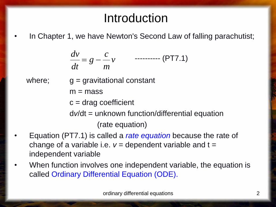
• In Chapter 1, we have Newton's Second Law of falling parachutist;

---------- (PT7.1)

where; g = gravitational constant

m = mass

c = drag coefficient

dv/dt = unknown function/differential equation

(rate equation)

• Equation (PT7.1) is called a rate equation because the rate of

change of a variable i.e. v = dependent variable and t =

independent variable

• When function involves one independent variable, the equation is

called Ordinary Differential Equation (ODE).

ordinary differential equations 2

vm

cg

dt

dv

• A partial differential equation (or PDE) involves two or more

independent variables.

• The fundamental laws of physics, mechanics, electricity, and

thermodynamics are usually based on empirical (experimentally)

observations that explain variations in physical properties and

states of systems.

• However, as described in previous chapter, many of differential

equations of practical significant cannot be solved using analytical

methods of calculus.

• Thus, this chapter covers important methods (Numerical

approach) for solving all engineering applications.

3 ordinary differential equations


Law Mathematical expression Variables & Parameters

Newton’s 2nd

law

of motion

Fourier’s heat

law

Fick’s law of

Diffusion

Faraday’s law

dv

dt

F

m

q k 'dT

dx

J Ddc

dx

VL Ldi

dt

V=velocity F=force m=mass q=heat flux k’=thermal conductivity T=temp. J=mass flux D=diffusion coefficient c=concentration VL=voltage drop L=inductance i=current

Table PT7.1 : Examples of fundamental laws in terms of rate of change of

variables (t = time, x = position)


Figure PT7.2 : The sequence of events in the application of ODEs for

engineering problem solving e.g. a falling parachutist

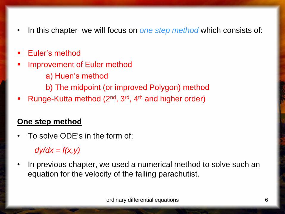
• In this chapter we will focus on one step method which consists of:

Euler’s method

Improvement of Euler method

a) Huen’s method

b) The midpoint (or improved Polygon) method

Runge-Kutta method (2nd, 3rd, 4th and higher order)

One step method

• To solve ODE's in the form of;

dy/dx = f(x,y)

• In previous chapter, we used a numerical method to solve such an

equation for the velocity of the falling parachutist.


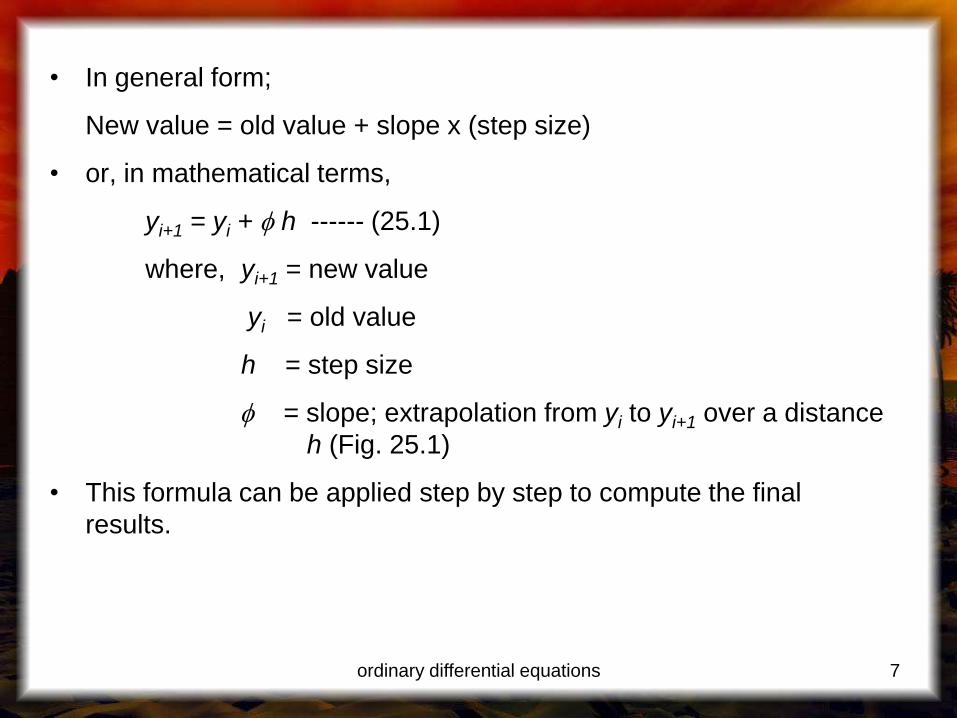
• In general form;

New value = old value + slope x (step size)

• or, in mathematical terms,

yi+1 = yi + h ------ (25.1)

where, yi+1 = new value

yi = old value

h = step size

= slope; extrapolation from yi to yi+1 over a distance

h (Fig. 25.1)

• This formula can be applied step by step to compute the final

results.


Step size = h

xi xi+1

y

x

hyy ii 1

Slope =

Figure 25.1: Graphical depiction of a one-step method


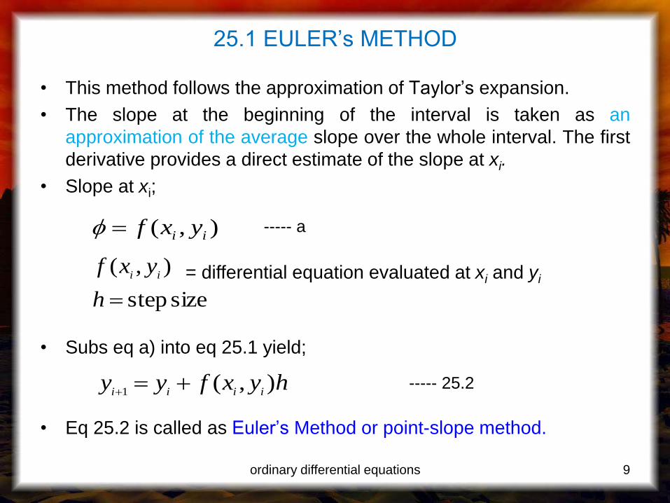
25.1 EULER’s METHOD

• This method follows the approximation of Taylor’s expansion.

• The slope at the beginning of the interval is taken as an

approximation of the average slope over the whole interval. The first

derivative provides a direct estimate of the slope at xi.

• Slope at xi;

• Subs eq a) into eq 25.1 yield;

• Eq 25.2 is called as Euler’s Method or point-slope method.

hyxfyyiiii),(

1


),( ii yxf

= differential equation evaluated at xi and yi

size step

),(

h

yxfii

----- a

----- 25.2

A new value of y is predicted using the slope (equal to the first

derivative at the original value of x) to extrapolate linearly over the

step size h


Fig. 25.2: Euler’s Method

Example 1: Use Euler’s method to numerically integrate:


5.820122 23 xxxdx

dy

from x = 0 to x = 4 with a step size of 0.5. Initial condition at x = 0 is

y = 1. Exact solution is given as;

y = -0.5x4 + 4x3 – 10x2 + 8.5x + 1

Example 1: Use Euler’s method to numerically integrate:


5.820122 23 xxxdx

dy

from x = 0 to x = 4 with a step size of 0.5. Initial condition at x = 0 is

y = 1. Exact solution is given as;

y = -0.5x4 + 4x3 – 10x2 + 8.5x + 1 Solution:

From Euler’s method equation;

1. Given; h = 0.5, x = 0 to 4, y(0) = 1

2. At x=0, y0 = 1

x=0.5, y0.5 = y0 + f (0,1) (0.5) = 1 + f (0,1) (0.5)

hyxfyy iiii ),(1

hyxfyy iiii ),(1

x yEuler

0

0.5

1.0

1.5

2.0

2.5

3.0

3.5

4.0

• Given;

• Therefore: f(0,1) = -2(0)3 + 12 (0)2 + 20(0) + 8.5 = 8.5

• From point 2,

y0.5 = 1 + f (0,1) (0.5) = 1 + (8.5) (0.5) = 5.25

Thus; y(0.5) = 1.0 + 8.5(0.5) = 5.25


5.820122 23 xxxdx

dy

%1.63%100x21875.3

03125.2

03125.225.521875.3

iserror true thethus,

21875.31)5.0(5.8)5.0(10)5.0(4)5.0(5.0

:is 0.5at xy newfor solution True

t

234

tE

y

3. At x = 1.0, y1 = y0.5 + f (0.5,5.25) (0.5) = 5.25 + f (0.5,5.25) (0.5)

• Therefore: f(0.5,5.25) = -2(0.5)3 + 12 (0.5)2 + 20(0.5) + 8.5 = 1.25

y1 = 5.25 + f(0.5, 5.25) (0.5)

Thus; y(1) = 5.25 + (1.25)(0.5) = 5.875


hyxfyy iiii ),(1

%8.95

875.2875.50.3

iserror true thethus,

0.31)1(5.8)1(10)1(4)1(5.0

is; 1at x solution The

t

234

tE

y


Table 25.1: Comparison true and approximation values

x ytrue yEuler t% Global t% Local 0.0 1.000 1.000 0.5 3.21875 5.250 -63.1 -63.1 1.0 3.000 5.875 -95.8 -128.0 1.5 2.21875 5.125 131.0 -1.41 2.0 2.000 4.500 -125.0 20.5 2.5 2.71875 4.7500 -74.7 17.3 3.0 4.000 5.8750 46.9 4.0 3.5 4.71875 7.1250 -51.0 -11.3 4.0 3.000 7.000 -133.3 -53.0

• The results for all data are compiled in table 25.1 and figure 25.3.

• Although the computation captures the general trend of the true

solution, the error is considerable.

• As discussed in the next section, this error can be reduced by using

a smaller step size

Fig. 25.3: Comparison of curve true solution with numerical solution

using Euler’s Method


Fig. 25.4: Comparison of curve true solution with numerical

solution using Euler’s Method


25.2 Improvements of Euler’s method

• Can be divided into 2 types;

a. Huen's Method

b. Mid-point Method (Improve Polygon Method)

25.2.1 Huen’s Method

• To improve the estimate of the slope.

• Involves the determination of two derivatives for the interval (h) at;

i. Initial Point

ii. End Point

• Then the two derivatives are averaged to obtain an improved

estimate of the slope for the entire interval, h.


• Recall Euler's Method; slop at beginning an interval;

y'i = (f (xi , yi ) -------- 25.12

• Used to extrapolate linearly to yi+1;

Note: for Euler's method we would stop at this point;

• However in Huen's Method yoi+1 is an intermediate prediction.

• Thus, equation 25.13 is called as Predictor equation and this

equation allowing the calculation of an estimated slope at the end of

interval:

hyxfy iii ),( 10

1

'

1


13.25 ),(1

hyxfyyiii

o

i

----- 25.14

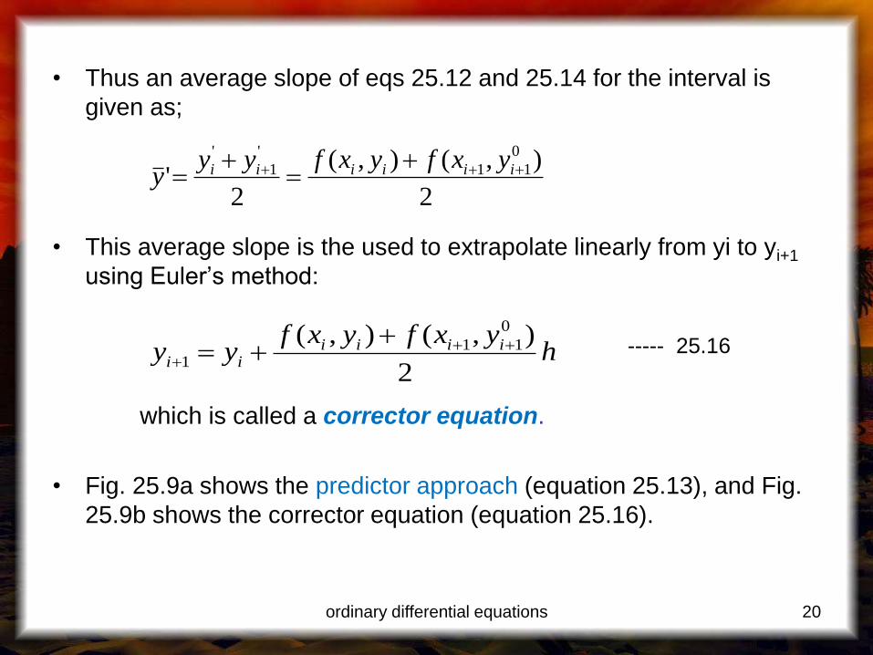
• Thus an average slope of eqs 25.12 and 25.14 for the interval is

given as;

• This average slope is the used to extrapolate linearly from yi to yi+1

using Euler’s method:

which is called a corrector equation.

• Fig. 25.9a shows the predictor approach (equation 25.13), and Fig.

25.9b shows the corrector equation (equation 25.16).

2

),(),(

2'

0

11

'

1

'

iiiiii yxfyxfyy

y

hyxfyxf

yy iiiiii

2

),(),( 0

111


----- 25.16

Fig. 25.9: (a) Predictor of Huen’s Method and (b) Corrector of Huen’s

Method


Termination Criterion:


%1001

1

11

j

i

j

i

j

ia

y

yy

j

iy 1

1

1

j

iy

where; Result from present iteration of corrector

Result from previous iteration of corrector

----- 25.17

Example 2: Use Huen’s method to integrate y’=4e 0.8x–0.5y from x = 0

to x = 4 with a step size of 1.0. The initial condition at x = 0 is y = 2.

Analytical solution for integral equation;

y’=4e 0.8x – 0.5y is;


xxx eeey 5.05.08.0 2)(3.1

4

Example 2: Use Huen’s method to integrate y’=4e 0.8x–0.5y from x = 0

to x = 4 with a step size of 1.0. The initial condition at x = 0 is y = 2.

Analytical solution for integral equation;

y’=4e 0.8x – 0.5y is;

Solution


xxx eeey 5.05.08.0 2)(3.1

4

This formula can be used to calculate true value/solution as shown in table

25.2;

(1 iteration each step) (15 iteration each step)

x ytrue yHeun t% yHeun t% 0 2.000 2.000 0.00 2.000 0.00 1 6.1946314 6.7010819 8.18 6.3608655 2.68 2 14.8439219 16.3197819 9.94 15.3022367 3.09 3 33.6771718 37.1992489 10.46 34.7432761 3.17 4 75.3389626 83.3377674 10.62 77.7350962 3.18

To calculate yHeun ; as Numerical Approach;

Given initial value; xi = 0, yi = 2

Predictor (eq. 25.13): yoi+1 = yi + f(xi , yi )h

= 2 + (1)

Step 1: f(xi , yi ) = f(0 , 2) = slope at point (xi , yi )

y’=4e 0.8x–0.5y

= 4e 0.8(0) – 0.5(2)

= 4-1 = 3

Step 2: predictor (eq 25.13);

yoi+1 = yi + f(xi , yi )h

= 2 + (1)

yoi+1 = 2 + 3(1) = 5


Thus, next point: xi+1 = 1 , yi+1 = 5

Step 3 : f(xi+1 , yo

i+1 )= f(1 , 5) = slope at point (xi+1 ,yo

i+1)

y’=4e 0.8x–0.5y

y’=4e 0.8(1)–0.5(5) = 6.402164

Step 4 : average slope

Step 5 : Corrector (eq 25.16);


2

),(),('

11

io

iii yxfyxfy

701082.42

)402164.6()3('

y

hyxfyxf

yyi

o

iii

ii2

),(),( 11

1

Thus;

Step 6 : repeat step 3 through step 5

Step 3: f(xi+1 , yi+1) = f(1 , 6.701082)

= 4e 0.8(1) - 0.5 (6.701082)

= 5.551622714


701082.6

)1(701082.42

1

hyy

or

o

%18.8

%1001946314.6

701082.61946314.6%

t

195.6

2)(3.1

4

2)(3.1

4

)1(5.0)1(5.0)1(8.0

5.05.08.0

eee

eeey xxx

Step 4 : slope average;

Step 5: corrector equation;

y1 = yo + h

= 2 + 4.275811357(1)

= 6.275811357

Thus;


275811357.42

551622714.53'

y

%31.1

%1001946314.6

275811.61946314.6%

t

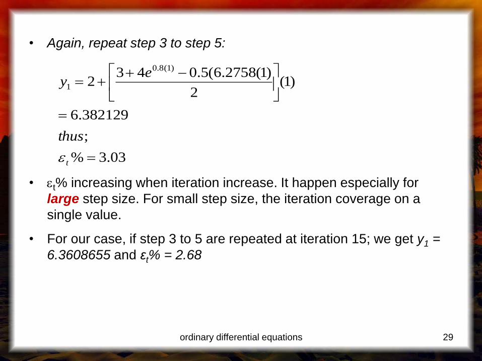
• Again, repeat step 3 to step 5:

• t% increasing when iteration increase. It happen especially for

large step size. For small step size, the iteration coverage on a

single value.

• For our case, if step 3 to 5 are repeated at iteration 15; we get y1 =

6.3608655 and εt% = 2.68


03.3%

;

382129.6

)1(2

)1(2758.6(5.0432

)1(8.0

1

t

thus

ey

Fig. 25.11: Comparison of true solution with numerical solution using

Euler's and Heun's method for y' = -2x3+12x2 -20x +8.5


25.2.2 Midpoint Method (Improved Polygon Method)

• Another simple modification of Euler’s method.

• This technique uses Euler's method to predict a value of y at

midpoint of interval as shown in Fig. 25.12 b).

• Thus the new value of y;

• Then, this predicted value is used to calculate a slope at the

midpoint:

which is assumed to represent a valid approximation of the average

slope for the entire interval.


2),(

2

1

hyxfyy iii

i

yi1

2

f (xi1

2

,yi1

2

)

----- 25.25

----- 25.26

Fig. 25.12 : Mid-point method for equations 25.24 and 25.27


Note: because yi+1

is not both sides,

the corrector (eq

25.16 cannot be

applied iteratively

to improve the

solution

• This slope is then used to extrapolate linearly from xi to xi+1 (Fig.

25.12).

Example 3: Use Midpoint method to solve this equation;

for range x = 0 to 2 and h = 0.5 where y(0) = 1.


27.25 ),(2

1

2

11

hyxfyyii

ii

y yx2 1.2y

Solution:

At x = 0, y = 1

At x = 0.5

(a)

(b) slope:


yi1

2

y i f (x i,y i)h

2

yi1

2

1 f (0,1)0.5

2

f (0,1) (1)(0)2 1.2(1) 1.2

yi1

2

1 (1.2)0.5

2 0.7

yi1

2

f (xi1

2

,yi1

2

) f (0.25,0.7)

f (0.25,0.7) (0.7)(0.25)2 1.2(0.7) 0.79625

c ) y i+1


yi1 yi f (xi1

2

,yi1

2

)h

yi1 1 (0.79625)(0.5) 0.601875

Ordinary Differential Equations Part 7

Documents

Transcript of Ordinary Differential Equations Part 7