ORCHIS: CONSISTENCY-DRIVEN DATA QUALITYMANAGEMENT IN SENSING SYSTEMS

by

KEWEI SHA

DISSERTATION

Submitted to the Graduate School

of Wayne State University,

Detroit, Michigan

in partial fulfillment of the requirements

for the degree of

DOCTOR OF PHILOSOPHY

2008

MAJOR: COMPUTER SCIENCE

Approved by:

Advisor Date

c©COPYRIGHT BY

Kewei Sha

2008

All Rights Reserved

ACKNOWLEDGEMENTS

During my pleasant work in the Mobile and Internet Systems Laboratory at Wayne

State University, I have got great help from many people. I would like to thank them

at this opportunity. First, I would like to thank my advisor, Dr. Weisong Shi, for his

invaluable advise, support, and discussion in my research. His vision, intelligence and

research experience are an inspiration and a model for me. I thank Dr. Loren Schwiebert,

Dr. Monica Brockmeyer and Dr. Cheng-zhong Xu to be on my dissertation committee and

their treasure comments and suggestions. I also thank Yong Xi, Guoxing Zhan and Safwan

Al-Omari, Sivakumar Sellamuthu, Junzhao Du for their great support. I am also thankful

to my friends, , Zhengqiang Liang, Hanping Lufei, Zhaoming Zhu, Hui Liu, Yonggen Mao,

Sharun Santhosh, Brandon Szeliga, Chenjia Wang and Tung Nguyen for their friendship

and support. Finally, I would like to thank my parents and my wife, Jie, for their great

support.

ii

TABLE OF CONTENTS

Chapter Page

ACKNOWLEDGEMENTS . . . . . . . . . . . . . . . . . . . . . . . . . . . . . . . . . ii

LIST OF TABLES . . . . . . . . . . . . . . . . . . . . . . . . . . . . . . . . . . . . . . viii

LIST OF FIGURES . . . . . . . . . . . . . . . . . . . . . . . . . . . . . . . . . . . . . ix

CHAPTER 1 Introduction . . . . . . . . . . . . . . . . . . . . . . . . . . . . . . . . . 1

CHAPTER 2 Overview of Sensing Systems . . . . . . . . . . . . . . . . . . . . . . . 8

2.1 Traditional Wireless Sensing Systems Overview . . . . . . . . . . . . . . . . . 10

2.1.1 Flat Structured Wireless Sensor Networks . . . . . . . . . . . . . . . . 11

2.1.2 Hierarchical Structured Wireless Sensor Networks . . . . . . . . . . . 12

2.1.3 Characteristics of Traditional Wireless Sensor Networks . . . . . . . . 13

2.1.4 Usage Pattern of Wireless Sensor Networks . . . . . . . . . . . . . . . 14

2.1.5 Communication Models in Wireless Sensor Networks . . . . . . . . . . 15

2.1.6 Two Query Protocols . . . . . . . . . . . . . . . . . . . . . . . . . . . 15

2.1.7 Routing Protocols . . . . . . . . . . . . . . . . . . . . . . . . . . . . . 16

2.2 Vehicular Networks . . . . . . . . . . . . . . . . . . . . . . . . . . . . . . . . . 17

2.2.1 Architecture of Vehicular Networks . . . . . . . . . . . . . . . . . . . . 19

2.2.2 Characters of Vehicular Networks . . . . . . . . . . . . . . . . . . . . . 20

iii

2.3 Healthcare Personal Area Networks . . . . . . . . . . . . . . . . . . . . . . . . 20

2.3.1 The Architecture of the SPA System . . . . . . . . . . . . . . . . . . . 22

2.3.2 Characters of the Healthcare Personal Area Networks . . . . . . . . . 24

CHAPTER 3 Related Work . . . . . . . . . . . . . . . . . . . . . . . . . . . . . . . . 26

3.1 Related Definition of Lifetime of Wireless Sensor Network . . . . . . . . . . . 26

3.2 Related Sensing Data Analysis . . . . . . . . . . . . . . . . . . . . . . . . . . 29

3.3 Related Energy Efficiency Design . . . . . . . . . . . . . . . . . . . . . . . . . 30

3.4 Related Data Consistency Models . . . . . . . . . . . . . . . . . . . . . . . . . 32

3.5 Related Adaptive Design in Wireless Sensor Networks . . . . . . . . . . . . . 35

3.6 Related Data management in Wireless Sensor Networks . . . . . . . . . . . . 37

3.7 Related MAC protocols in Wireless Sensor Networks . . . . . . . . . . . . . . 38

3.8 Related Deceptive Data Detection Protocols . . . . . . . . . . . . . . . . . . . 39

CHAPTER 4 Orchis: A Consistency-Driven Data Quality Management Framework . 43

CHAPTER 5 Modeling the Lifetime of Sensing Systems . . . . . . . . . . . . . . . . 49

5.1 Assumptions and Definitions of Parameters . . . . . . . . . . . . . . . . . . . 50

5.2 Definition of Remaining Lifetime of Sensors . . . . . . . . . . . . . . . . . . . 50

5.3 Probability of ith Message Through the jth Sensor . . . . . . . . . . . . . . . 52

5.4 Remaining Lifetime of Sensors in Unicast using Traditional . . . . . . . . . . 54

5.5 Remaining Lifetime of Sensors in Broadcast using Traditional . . . . . . . . . 55

5.6 Remaining Lifetime of Sensors in IQ . . . . . . . . . . . . . . . . . . . . . . . 55

5.7 Importance of Different Sensor Nodes . . . . . . . . . . . . . . . . . . . . . . 56

5.8 Remaining Lifetime of the Whole Sensor Network . . . . . . . . . . . . . . . . 57iv

5.9 Analytical Comparison: Traditional vs. IQ . . . . . . . . . . . . . . . . . . 59

5.10 Simulation Verification . . . . . . . . . . . . . . . . . . . . . . . . . . . . . . . 61

5.10.1 Energy Consumption . . . . . . . . . . . . . . . . . . . . . . . . . . . . 61

5.10.2 Simulation results of RLSN . . . . . . . . . . . . . . . . . . . . . . . . 62

5.10.3 Simulation results of LSN . . . . . . . . . . . . . . . . . . . . . . . . . 64

CHAPTER 6 Quality-oriented Sensing Dada Analysis . . . . . . . . . . . . . . . . . 66

6.1 Background . . . . . . . . . . . . . . . . . . . . . . . . . . . . . . . . . . . . 67

6.2 Quality-Oriented Sensing Data Analysis . . . . . . . . . . . . . . . . . . . . . 70

6.2.1 Time Series Analysis for Individual Parameter . . . . . . . . . . . . . 70

6.2.2 Multi-Modality and Spatial Sensing Data Analysis . . . . . . . . . . . 85

CHAPTER 7 Modeling Data Consistency in Sensing Systems . . . . . . . . . . . . . 89

7.1 Consistency Requirements Analysis . . . . . . . . . . . . . . . . . . . . . . . . 89

7.2 Consistency Models . . . . . . . . . . . . . . . . . . . . . . . . . . . . . . . . 92

7.2.1 Data Format . . . . . . . . . . . . . . . . . . . . . . . . . . . . . . . . 92

7.2.2 Consistency Models for Individual Data . . . . . . . . . . . . . . . . . 94

7.2.3 Consistency Models for Data Streams . . . . . . . . . . . . . . . . . . 96

7.3 APIs for Managing Data Consistency . . . . . . . . . . . . . . . . . . . . . . . 100

CHAPTER 8 An Adaptive Lazy Protocol . . . . . . . . . . . . . . . . . . . . . . . . 104

8.1 ALEP: An Adaptive, Lazy, Energy-efficient Protocol . . . . . . . . . . . . . . 104

8.1.1 Rationale . . . . . . . . . . . . . . . . . . . . . . . . . . . . . . . . . . 104

8.1.2 Two Types of Data Dynamics . . . . . . . . . . . . . . . . . . . . . . . 105

8.1.3 Model for Data Dynamics . . . . . . . . . . . . . . . . . . . . . . . . . 106v

8.1.4 Adapting the Sample Rate . . . . . . . . . . . . . . . . . . . . . . . . 109

8.1.5 Keeping Lazy in Transmission . . . . . . . . . . . . . . . . . . . . . . . 110

8.1.6 Aggregating and Delaying Delivery . . . . . . . . . . . . . . . . . . . . 111

8.1.7 Discussions . . . . . . . . . . . . . . . . . . . . . . . . . . . . . . . . . 111

8.2 Performance Evaluation: Simulation . . . . . . . . . . . . . . . . . . . . . . . 112

8.2.1 Simulation Setup and Evaluation Metrics . . . . . . . . . . . . . . . . 113

8.2.2 Number of Delivered Messages . . . . . . . . . . . . . . . . . . . . . . 115

8.2.3 Data Inconsistency Factor . . . . . . . . . . . . . . . . . . . . . . . . . 116

8.2.4 Tradeoff between Energy Efficiency and Data Consistency . . . . . . . 119

8.3 Performance Evaluation: Prototype . . . . . . . . . . . . . . . . . . . . . . . . 124

8.3.1 SDGen: Sensor Data Generator . . . . . . . . . . . . . . . . . . . . . . 125

8.3.2 Comparison Number of Delivered Messages . . . . . . . . . . . . . . . 126

8.3.3 Comparison of Energy Consumption . . . . . . . . . . . . . . . . . . . 127

8.3.4 Comparison of Samplings . . . . . . . . . . . . . . . . . . . . . . . . . 129

8.3.5 Comparison of Data Inconsistency Factor . . . . . . . . . . . . . . . . 130

8.3.6 Discussions . . . . . . . . . . . . . . . . . . . . . . . . . . . . . . . . . 131

CHAPTER 9 D4: Deceptive Data Detection in Dynamic Sensing Systems . . . . . . 133

9.1 Necessity of Deceptive Data Detection and Filtering . . . . . . . . . . . . . . 134

9.1.1 Deceptive Data Definition . . . . . . . . . . . . . . . . . . . . . . . . . 135

9.1.2 Insufficiency of Previous Approaches . . . . . . . . . . . . . . . . . . . 137

9.2 A Framework to Detect Deceptive Data . . . . . . . . . . . . . . . . . . . . . 138

9.2.1 Quality-Assured Aggregation & Compression . . . . . . . . . . . . . . 139

9.2.2 The RD4 Mechanism . . . . . . . . . . . . . . . . . . . . . . . . . . . 140vi

9.2.3 Self-Learning Model Based Detection . . . . . . . . . . . . . . . . . . . 140

9.2.4 Spatial-Temporal Data Recognition . . . . . . . . . . . . . . . . . . . 141

9.2.5 Discussion . . . . . . . . . . . . . . . . . . . . . . . . . . . . . . . . . . 142

9.3 Role-differentiated Cooperative Deceptive Date Detection and Filtering . . . 143

9.4 RD4 in Vehicular Networks . . . . . . . . . . . . . . . . . . . . . . . . . . . . 147

9.4.1 Role Definition in Vehicular Networks . . . . . . . . . . . . . . . . . . 148

9.4.2 False Accident Report Detection . . . . . . . . . . . . . . . . . . . . . 149

9.5 Performance Evaluation . . . . . . . . . . . . . . . . . . . . . . . . . . . . . . 151

9.5.1 Simulation Setup . . . . . . . . . . . . . . . . . . . . . . . . . . . . . . 151

9.5.2 Effectiveness of RD4 . . . . . . . . . . . . . . . . . . . . . . . . . . . . 153

9.5.3 Efficiency of RD4 . . . . . . . . . . . . . . . . . . . . . . . . . . . . . . 154

9.5.4 Message Complexity . . . . . . . . . . . . . . . . . . . . . . . . . . . . 157

9.5.5 Effect of Maximum Confidential Scores . . . . . . . . . . . . . . . . . 157

CHAPTER 10 Conclusions and Future Work . . . . . . . . . . . . . . . . . . . . . . . 160

10.1 Conclusion . . . . . . . . . . . . . . . . . . . . . . . . . . . . . . . . . . . . . 160

10.2 Future Work . . . . . . . . . . . . . . . . . . . . . . . . . . . . . . . . . . . . 160

10.2.1 Complete and Extend the Orchis Framework . . . . . . . . . . . . . . 161

10.2.2 Privacy and Security in Sensing Systems . . . . . . . . . . . . . . . . . 161

10.2.3 Sensing System Applications in Healthcare Systems . . . . . . . . . . 162

REFERENCES . . . . . . . . . . . . . . . . . . . . . . . . . . . . . . . . . . . . . . . . 163

AUTOBIOGRAPHICAL STATEMENT . . . . . . . . . . . . . . . . . . . . . . . . . . 185

vii

LIST OF TABLES

Table Page

5.1 A list of variables used in Chapter 5. . . . . . . . . . . . . . . . . . . . . . . . 51

5.2 Comparison of the remaining lifetime of different nodes in different locations. 59

5.3 Comparison of the remaining lifetime of the whole sensor network. . . . . . . 60

5.4 Simulation parameters. . . . . . . . . . . . . . . . . . . . . . . . . . . . . . . . 61

7.1 APIs for data consistency management. . . . . . . . . . . . . . . . . . . . . . 103

viii

LIST OF FIGURES

Figure Page

2.1 Flat structured wireless sensor networks. . . . . . . . . . . . . . . . . . . . . . 11

2.2 Hierarchical structured wireless sensor networks. . . . . . . . . . . . . . . . . 12

2.3 A typical authentication scenario. . . . . . . . . . . . . . . . . . . . . . . . . . 18

2.4 The architecture of the SPA system. . . . . . . . . . . . . . . . . . . . . . . . 22

4.1 An overview of the Orchis framework. . . . . . . . . . . . . . . . . . . . . . . 44

5.1 Message propagation in sensor networks. . . . . . . . . . . . . . . . . . . . . . 53

5.2 An example of the importance of different sensors, assuming the data sink is

located at the low-left corner. . . . . . . . . . . . . . . . . . . . . . . . . . . 56

5.3 Comparison of energy consumption in Traditional and in IQ using GPSR. . 62

5.4 Comparison of RLSN by using Traditional and IQ. . . . . . . . . . . . . . . 63

5.5 Comparison of LSN by using Traditional and IQ. . . . . . . . . . . . . . . . 64

6.1 Lake Winnebago Watershed. . . . . . . . . . . . . . . . . . . . . . . . . . . . 68

6.2 St. Clair River and Detroit River. . . . . . . . . . . . . . . . . . . . . . . . . 69

6.3 Detected patterns and the number of appearance in gauge G5. . . . . . . . . 75

6.4 Pattern reappearance ratio with zero endurance interval. . . . . . . . . . . . . 76

6.5 Pattern reappearance ratio with increased endure interval. . . . . . . . . . . . 76

6.6 CDF of pattern length of Voltage. . . . . . . . . . . . . . . . . . . . . . . . . 77

6.7 CDF of pattern length: of water level. . . . . . . . . . . . . . . . . . . . . . . 77

ix

6.8 CDF of pattern length of precipitation. . . . . . . . . . . . . . . . . . . . . . 78

6.9 The number of appearances for each numerical values of voltage. . . . . . . . 78

6.10 The number of appearances for each numerical values of water level. . . . . . 79

6.11 The number of appearances for each numerical values of precipitation. . . . . 79

6.12 Numerical reappearance ratio with endurance interval [0.00, 0.00]. . . . . . . 80

6.13 Numerical reappearance ratio with increased endurance interval. . . . . . . . 81

6.14 Detected out-of-range readings. . . . . . . . . . . . . . . . . . . . . . . . . . . 82

6.15 Limit control of G3’s hourly water level changes. . . . . . . . . . . . . . . . . 83

6.16 Out-of-Limit ratio for hourly water level changes. . . . . . . . . . . . . . . . . 83

6.17 Conflict ratio of water level and precipitation. . . . . . . . . . . . . . . . . . . 85

6.18 Spatial correlation of water level. . . . . . . . . . . . . . . . . . . . . . . . . . 86

6.19 Spatial correlation of precipitation. . . . . . . . . . . . . . . . . . . . . . . . . 86

7.1 A three-dimension view of consistency requirements. . . . . . . . . . . . . . . 91

8.1 Data dynamics with the time. . . . . . . . . . . . . . . . . . . . . . . . . . . . 107

8.2 Data dynamics in different location. . . . . . . . . . . . . . . . . . . . . . . . 108

8.3 Adapting data sampling rate. . . . . . . . . . . . . . . . . . . . . . . . . . . . 109

8.4 A tree-structured sensor network used in the simulation and prototype. The

numbers next to each node is node ID or Mote ID. . . . . . . . . . . . . . . . 113

8.5 Number of delivered messages without aggregation. . . . . . . . . . . . . . . . 117

8.6 Number of delivered messages with aggregation. . . . . . . . . . . . . . . . . . 118

8.7 Data inconsistency factor. . . . . . . . . . . . . . . . . . . . . . . . . . . . . . 119

8.8 Number of messages with variant temporal bound using Alep. . . . . . . . . . 120

8.9 Number of messages with different numerical consistency bound. . . . . . . . 121x

8.10 Data inconsistency factor with variant value bound using Alep. . . . . . . . . 122

8.11 Number of delivered messages with variant maximum data sampling rate. . . 123

8.12 State transition diagram of sensor data generator. . . . . . . . . . . . . . . . 125

8.13 Comparison of number of messages delivered by Layer one Motes. . . . . . . . 127

8.14 Comparison of voltage dropping of different protocols. . . . . . . . . . . . . . 128

8.15 Comparison of received data at the sink with real data. Note that the

SQUARE shape represents the values of real data and the DIAMOND shape

shows the value of collected data. . . . . . . . . . . . . . . . . . . . . . . . . . 129

8.16 Comparison of data inconsistency factor. . . . . . . . . . . . . . . . . . . . . . 131

9.1 An overview of the framework to detect and filter deceptive data. . . . . . . . 139

9.2 A snapshot of vehicular network simulator. . . . . . . . . . . . . . . . . . . . 152

9.3 Recall of false accident reports. . . . . . . . . . . . . . . . . . . . . . . . . . . 153

9.4 Recall of true accident reports. . . . . . . . . . . . . . . . . . . . . . . . . . . 154

9.5 Confirmation time of true accident reports. . . . . . . . . . . . . . . . . . . . 155

9.6 Propagation range of true accident reports. . . . . . . . . . . . . . . . . . . . 155

9.7 Message complexity of RD4. . . . . . . . . . . . . . . . . . . . . . . . . . . . . 157

9.8 Effect of maximum confidential scores. . . . . . . . . . . . . . . . . . . . . . . 158

xi

1

CHAPTER 1

INTRODUCTION

As new fabrication and integration technologies reduce the cost and size of micro-sensors

and wireless sensors, we will witness another revolution that facilitates the observation and

control of our physical world [Akyildiz et al., 2002,Estrin et al., 2002,Estrin et al., 1999,Es-

trin et al., 2003, Pottie and Kaiser, 2000] just as networking technologies have changed

the way individuals and organizations exchange information. Micro sensors such as Motes

from Intel and Crossbow [crossbow, ] have been developed to make wireless sensor network

applications possible; TinyOS [Hill et al., 2000, Levis et al., 2003] has been designed to

provide adequate system support to facilitate sensor node programming; and finally, sev-

eral efficient protocols have been proposed to make the sensor system workable. Several

applications, such as habitat monitoring [Szewczyk et al., 2004a, Szewczyk et al., 2004b],

ZebraNet [Sadler et al., 2004], Counter-sniper system [Simon et al., 2004], environment

sampling [Batalin et al., 2004], target tracking [Shrivastava et al., 2006] and structure mon-

itoring [Xu et al., 2004], have been launched, showing the promising future of wide range of

applications of wireless sensor networks (WSNs). Recently, several novel architectures have

been funded by NSF, such as SNA [SNA, ] at UC Berkeley, Tenet [Gnawali et al., 2006] at

UCLA/USC, COMPASS [COMPASS, ] at Rice, and Wavescope [Wavescope, ] at MIT.

Sensing and communication technologies together broaden the way we observe and serve

the world, thus in recent several years, more and more physical systems start to integrate

those latest technologies into their systems so that they can take advantage of power of sens-

ing and communication [Atkins, 2006, Campbell et al., 2006, Douglas et al., 2006, Garrett

et al., 2006,Krause et al., 2008,Srivastava et al., 2006], which not only brings new opportu-

nities to extend the application of traditional wireless sensing systems but also brings new

2

challenges in designing of the extended wireless sensing systems. For example, after sensors

and communication components are installed on vehicles, vehicles can form a extremely

large-scale high-mobility ad hoc sensing system, Vehicular Networks. Based on vehicular

networks, real-time traffic information and interested environmental information can be col-

lected, and various services such as safety services, dynamic routing services can be deployed.

With more and more traditional biomedical sensors equipped with wireless communication

components, those sensors together with smart phones and the existing cellular or WLAN

networks form a healthcare personal area sensing network, which can collect biophysical

data from the patient and perform the function of long-term body condition monitoring.

Among all aforementioned systems, we find that different system architectures as well as

variant system protocols are requires to cater the requirements of different wireless sensing

system applications. As a result, an application-specific approach will be explored in those

system design. Whereas, we also envision that, among all aforementioned systems, the

success of those wireless sensing system applications is nonetheless determined by whether

those wireless sensing systems can provide a high quality stream of data over a long period.

The inherent feature of deployment of those wireless sensing systems in a malicious or

uncontrolled environment, however, imposes challenges to the underlying systems. These

challenges are further complicated by the fact that sensor systems are usually seriously

energy constrained. However, this problem is largely neglected in previous research, which

usually focuses on devising techniques to save the sensor node energy and thus extend the

lifetime of the whole wireless sensing systems. However, with more and more deployments

of real sensing systems, in which the main function is to collect interesting data and to

share with peers, data quality management has been becoming a more important issue in

the design of sensor systems. In this dissertation, we envision that data quality management

should be integrated in an energy-efficient all sensing system design.

We argue that the quality of data should reflect the timeliness and accuracy of collected

data that are presented to interested recipients who make the final decision based on these

3

data. Therefore, new protocols are needed to collect both fresh enough and accurate enough

data in an efficient way, and the task of deceptive data detection and filtering plays a vital

role in the success of data collection. We believe that security using traditional cryptography

mechanisms, such as encryption for confidentiality, hashing digest for message integrity, are

definitely important and necessary, but not enough to detect deceptive data resulting from

data collection and data transmission through multi-hop wireless links. In this dissertation,

we undertake a novel approach that detects and filters deceptive data through considering

the consistency requirements of data, and study the relationship between the quality of data

and the multi-hop communication and energy-efficient design of wireless sensing systems.

To achieve the goal of collecting high quality data in an efficient way, we first analyze a set

of real-world sensing data from an environmental monitoring application, then we formally

define a new metric, data consistency, against which the quality of data is evaluated and

the deceptive data is detected and filtered. Intuitively most people think that the high

requirements of data quality, the more energy will be consumed. However, based on our

observation from sensing data analysis, we find that in most cases the energy could be

saved if we consider data consistency and data dynamics together, which inspired us to

attack the problem from the prospective of data consistency and data dynamics, and exploit

the data consistency in the system protocol design. Second, we propose a set of APIs to

manage the consistency and devise an adaptive protocol to integrate data dynamics with

data consistency. Moreover, we design a general framework to detect and filter deceptive

data so that the quality of the collected data can be largely improved. Finally, energy

efficiency is still one of major design goals in our design. Thus, we argue that a good metric

is necessary to systematically evaluate the energy efficiency performance of the proposed

protocols.

All these models and protocols are integrated in a framework named Orchis, which

basically has six components, including an analysis to the characteristics of the sensing

data from an environmental application, a set of data consistency models customized to

4

wireless sensing systems, a set of APIs to management the quality of collected data, an

adaptive protocol for data sampling, a framework to detect and filter deceptive data, and a

formal model for the lifetime of the wireless sensing system to evaluate the energy efficiency

performance of the protocols. Specifically, we have investigated the following six research

problems in this dissertation:

1. Model lifetime for wireless sensor networks. Although in the extended sensing sys-

tems, the energy constraint is not as severe as that in traditional sensing systems,

energy efficiency is still one of the major goals in sensing system design; We propose

a novel model to formally define the lifetime of a wireless sensor network based on en-

ergy by considering the relationship between individual sensors and the whole sensor

network, the importance of different sensors based on their positions, the link quality

in transmission, and the connectivity and coverage of the sensor network. Based on

our model, we have compared two types of query protocols, the direct query protocol

and the indirect query protocol, in terms of mathematical analysis. Then, a compre-

hensive simulation is done to validate the correctness of the mathematical analysis

built on our model. The simulation results shows the correctness of our model.

2. Analyze the characteristics of a set of sensing data collected in an environmental

monitoring application it is crucial to carefully analyze the collected sensing data,

which not only helps us understand the features of monitored field, but also unveil

any limitations and opportunities that should be considered in future sensor system

design. In this dissertation, we take an initial step and analyze one-month sensing data

collected from a real-world water system surveillance application, focusing on the data

similarity, data abnormality and failure patterns. Based on our analysis, we find that,

(1) Information similarity, including pattern similarity and numerical similarity, is very

common, which provides a good opportunity to trade off energy efficiency and data

quality; (2) Spatial and multi-modality correlation analysis provide a way to evaluate

5

data integrity and to detect conflicting data that usually indicates appearances of

sensor malfunction or interesting events.

3. Model the data consistency in wireless sensor networks. Like those in traditional

distributed systems, consistency models in wireless sensing systems are proposed for

evaluating the quality of the collected data. Based on our knowledge, we are the first

to raise the data quality problem in wireless sensing systems. In this dissertation, we

propose a novel metric, data consistency, to evaluate the data quality. Our consistency

models consider three perspectives of consistency: temporal, numerical, and frequency,

covering both individual data and data streams. Furthermore, we also defined spacial

and multi-modality consistency for sensing data.

4. Develop a set of APIs to manage data consistency and handle the deceptive data. A

set of APIs are designed to distribute data consistency requirements to the monitor-

ing area when the sensor network is deployed. Later on, the consistency requirement

should be updated according to the observed data consistency from recent collected

data. These APIs are essential and enable application scientists to disseminate con-

sistent requirements, check consistency status, manage consistency requirements, and

detect and filter deceptive data. Also, these APIs provide interfaces for lower layer

data collection protocols to efficiently transfer the data to the sink.

5. Devise an adaptive protocol to detect deceptive data and improve the quality of col-

lected data and take advantage of data consistency by considering data dynamics. We

observe that data consistency and energy efficiency are closely related to data dynam-

ics. Thus, models for data dynamics are designed. The protocol that automatically

adapts the data sampling rate according to the data dynamics in the data field and

data consistency requirements from the application is proposed to improve the quality

of collected data and to save energy. As a result, energy can be saved when the data

dynamics are low or when data consistency requirements are low. Furthermore, the

6

zoom-in feature of the adaptive protocol helps us not only to detect interests data

changes which usually means abnormal data or interested event, but also to detect

deceptive data and improve the quality of sensed data significantly.

6. Design a deceptive data detection protocol to support data consistency and filtering of

deceptive data. The quality of the collected data are mainly affected by the deceptive

data, which usually comes from two sources, wrong readings resulted from inaccurate

sensing components and unreliable wireless communication, and false data inserted

by malicious attackers. In this dissertation, we propose a general framework to de-

tect the deceptive data from the view point of data itself. Basically, we try to filter

two types of deceptive data, redundant data and false data. In our framework, those

two types of deceptive data are treated differently. Quality-assured aggregation and

compression is used to detect and filter redundant data, while role-differentiated coop-

erative deceptive data detection and filtering and self-learning model-based deceptive

data detection and filtering are utilized to filter false data. Finally, when both types

of deceptive data are checked and recognized after the data are delivered to a cen-

tral server, a spatial-temporal data consistency checking can be performed to further

detect and filter the remaining deceptive data.

The proposed framework is close-loop feedback control to manage data quality of the

collected data, thus it is a general framework that can be used in all kinds of sensing systems

and data quality can be bounded by consistency models or application requirements. With

Orchis framework, we can expect that high quality data can be collected in an efficient way.

The the efficiency and effectiveness of proposed protocols and models in the framework are

validated by both simulation and prototypes, which can be found in the different chapters

in this dissertation.

The rest of the dissertation is organized as follows. Background about wireless sensor

networks and some related work are listed in Chapter 2. Related work is listed in Chapter 3.

7

Chapter 4 describes the Orchis framework and an overview of all the components in Orchis.

In Chapter 6, we analyze the characteristics of the sensing data collected from a real-

life environmental monitoring application. Model for lifetime of wireless sensor networks

is formally defined in Chapter 5 and a set of consistency models is formally defined in

Chapter 7. Chapter 8, an adaptive, lazy, energy-efficiency protocol is proposed, followed

by the design of a framework to detect and filter deceptive data in Chapter 9. Finally,

conclusion is drawn and future work is listed in Chapter 10.

8

CHAPTER 2

OVERVIEW OF SENSING SYSTEMS

Integrating the latest technology of sensing, wireless communication, embedded systems,

distributed systems, and networking, sensing systems become a very hot research area for

both scientists and engineers. A lot of applications have been developed based on sensing

systems. Originally, sensing systems are mostly applied in environmental applications such

as [Estrin et al., 2003, Martinez et al., 2004]and [Batalin et al., 2004]. When sensors are

equipped at vehicles and other devices, the traditional sensing systems have been extended

to more complicated sensing systems, including Vehicular Networks and healthcare personal

area networks. From the evolution of the sensing systems, we find several trends in the

progress, as listed as follows.

First, one significant difference between the traditional sensing systems and the extended

sensing systems is the targeting applications. The traditional sensing systems are mostly

applied in scientific applications such as environmental monitoring, but the extended sensing

systems are more targeting to personal and social applications, and also they are targeting to

more commercial applications. As a result, the data flow is one direction for collecting data

in traditional sensing systems, while they are two directions for collecting and distributing

data in the extended sensing systems because of the requirements on data sharing. In

addition, because of the involve of persons, security and privacy play a bigger concern in the

extended sensing system design. Second, the traditional sensing system are usually applied

for single dedicated application, while the extended sensing system will mostly be applied by

an integration of multiple applications. For example, an environmental monitoring sensing

system will focus on collecting data from monitoring field, while a vehicular network can

9

be used both in collecting real-time road information and in deploying a lot of location-

based services. Third, sensors in the traditional sensing systems are mostly static, while in

the extended sensing systems such as vehicular networks and personal area networks, most

sensors have high mobility due to the movement of the vehicles and persons. The mobility

of those sensors introduces both challenges and opportunities. Forth, in most environmental

applications, sensors are distributed in an uncontrolled area and energy efficiency is a big

problem. In the extended sensing systems, sensors are more likely to be deployed in a

controlled space, and some sensors have chance to be recharged, so although energy efficiency

is still a big design concern in extended sensing systems, the limitation on power supply

is not as severe as that in traditional sensing systems. Last but not least, in traditional

sensing systems, most sensors are homogeneous, while they are more heterogeneous in the

extended sensing systems. Furthermore, the extended sensing systems will have more closer

entanglement with the current existing networks such as Internet and Cellular Networks,

thus, it more heterogeneous communication protocols will be involved.

Because of the different focuses and requirements in various sensing applications and

various sensing systems, the design of the sensing system usually follows an application

specific approach, i.e., the system design is largely adapted to the requirements of the ap-

plications; however, we argue that there are still some common concerns in sensing system

design. For example, energy efficiency is one of the most important concerns in sensing sys-

tem design, because most sensors are battery powered. Although energy efficiency problem

has been relieved somehow in the extended sensing systems such as vehicular networks, it

is still a concern even in the design of those systems. Security and privacy are another big

concerns in the system design, especially in the extended sensing systems such as healthcare

personal-area networks, in which privacy may be the key to the acceptance of those sensing

systems. Furthermore, we argue that the most important concern in all sensing system

design should be data quality management, because the major function of sensing system

10

is to collect interested high quality data. In this dissertation, we try to integrate the data

quality management in an energy efficient sensing systems design.

Having known that there are different sensing systems, such as traditional sensing sys-

tems, and the extended sensing systems. Here we give an overview of those existing sensing

systems, including traditional sensing systems, vehicular networks, and healthcare personal-

area sensing networks. In the following sections, we will introduce the architecture and the

characteristics of them one by one.

2.1 Traditional Wireless Sensing Systems Overview

Traditional wireless sensing systems usually have two ways to organize the sensors in the

wireless sensor network. One is a flat structured wireless sensor network. The other is a

hierarchical structured wireless sensor network. The overview of these two types of networks

are listed in next two subsections.

Traditional wireless sensor networks can be applied in various scenarios. We list several

typical applications of the traditional sensing systems. For instance, they are used a lot in

passive monitoring applications such as traffic monitoring [Skordylis et al., 2006], battle field

monitoring [Bokareva et al., 2006,Sha and Shi, 2006b] and environment monitoring [Batalin

et al., 2004, Szewczyk et al., 2004b]. They are also used a lot in event-driven applications

like enemy detection, fire detection, and object tracking. Furthermore, they are very useful

in active querying applications, e.g., you can check the condition of the object you are

monitoring by sending it some queries. These different applications may have various specific

application requirements to the sensor system design. Thus, traditional wireless sensor

networks can be heterogenous systems because of specific application requirements, i.e., in

different applications different types of devices may be used as sensors. For example, the

motes from CrossBow and Intel can be used as sensors; the RFID readers can act as sensors

and collect information from RFID; moreover, the device like web-camera can be used as

sensors to monitor the activity of the area. In addition, sensors can be equipped with GPS

11

devices to get accurate location. The two major structure of the sensing systems are listed

as follows.

2.1.1 Flat Structured Wireless Sensor Networks

Mote

Gateway/Sink

Mote

Mote

Remote TaskManagerLocal Server

Figure 2.1: Flat structured wireless sensor networks.

A flat structured wireless sensor network usually consists of a set of sensors, a gateway

or sink and some other powerful machines as shown in Figure 2.1. Each sensor has the

similar capability of computation, communication, and sensing. With the ability of wireless

communication, sensors can self-organized into a network that usually has flexible structure.

Each sensor in the sensor network may perform as a router so that it forwards message for

others. In the data collection process in sensor networks, the data is first sampled at each

sensor, then it is transferred to a gateway or a sink, which is usually a more powerful

device, in a multi-hop way. The data are further delivered to some local servers such as

local servers like desktops and Laptops, which have more powerful computing capability

and larger storage, or remote machines via Internet, which locate far away from the sensor

network and act as remote task management.

12

2.1.2 Hierarchical Structured Wireless Sensor Networks

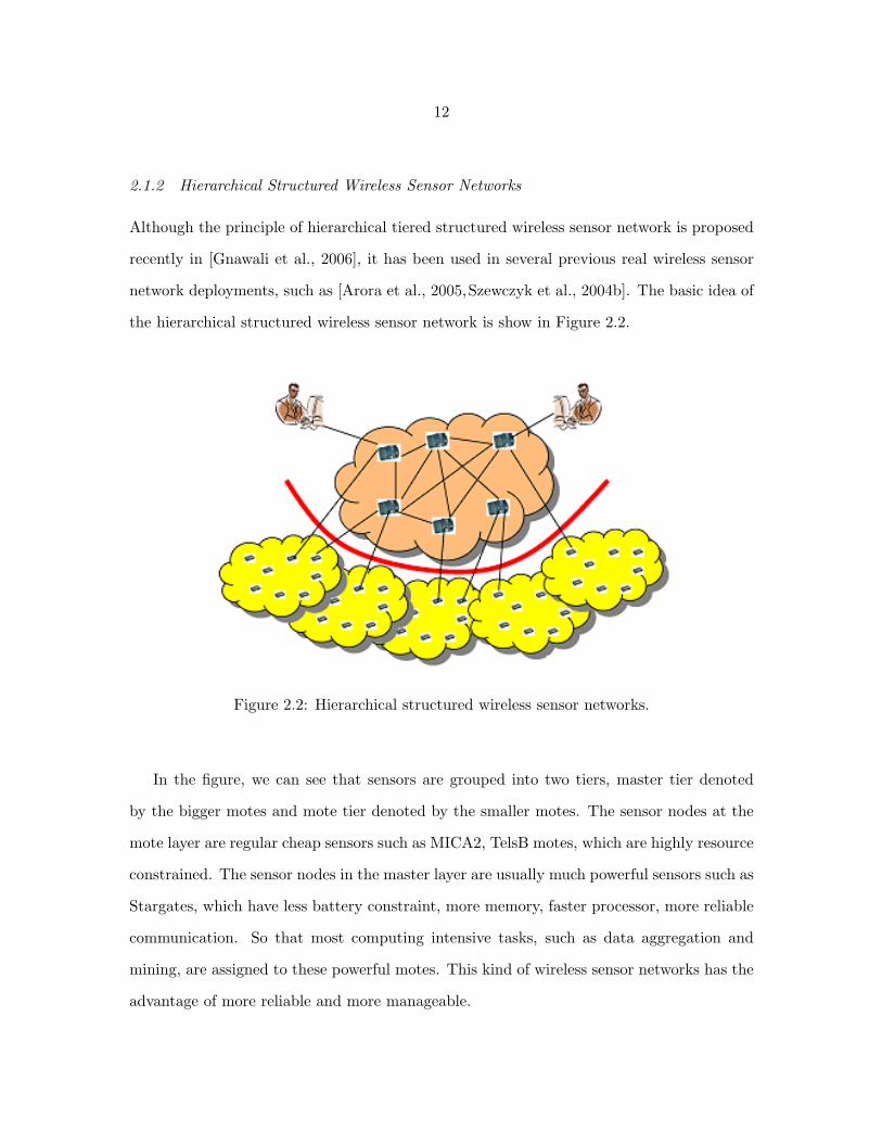
Although the principle of hierarchical tiered structured wireless sensor network is proposed

recently in [Gnawali et al., 2006], it has been used in several previous real wireless sensor

network deployments, such as [Arora et al., 2005,Szewczyk et al., 2004b]. The basic idea of

the hierarchical structured wireless sensor network is show in Figure 2.2.

Figure 2.2: Hierarchical structured wireless sensor networks.

In the figure, we can see that sensors are grouped into two tiers, master tier denoted

by the bigger motes and mote tier denoted by the smaller motes. The sensor nodes at the

mote layer are regular cheap sensors such as MICA2, TelsB motes, which are highly resource

constrained. The sensor nodes in the master layer are usually much powerful sensors such as

Stargates, which have less battery constraint, more memory, faster processor, more reliable

communication. So that most computing intensive tasks, such as data aggregation and

mining, are assigned to these powerful motes. This kind of wireless sensor networks has the

advantage of more reliable and more manageable.

13

2.1.3 Characteristics of Traditional Wireless Sensor Networks

Although sensor networks are a special type of traditional distributed systems and mobile

ad-hoc networks, there are several major differences between wireless sensor networks and

traditional distributed systems. These differences are listed as following.

• The number of sensor nodes is much more than that in the other systems, i.e., it is

common to have thousands of sensors in one sensor network.

• Sensor nodes are usually deployed from an aircraft in a rapid, ad hoc manner, so that

the deployment and the topology of the sensors are out of control at most time.

• The sensor nodes are usually densely distributed but they are more likely to fail due

to the physical failure or out of power supply.

• Sensors are resource constrained devices which have limited bandwidth, computation

capability, and small memory, which probably will disappear gradually with the devel-

opment of new fabrication technologies. The most significant difference between the

wireless sensor network and the traditional distributed system is the limited energy

supply of sensors, which is believed to be a long term problem.

• It is difficult to replace failed sensors in the sensor network because sensors may be

deployed to an area where human beings cannot access, such as in hazardous area and

waste containment cover clay soil.

• Sensor networks are application specific systems, which are applied in various scenarios

so that they may have different design goals and requirements.

• Data aggregation is a common strategy used in wireless sensor networks to reduce

the total amount of data traffic. Thus, aggregation is much more in wireless sensor

networks than in traditional distributed systems.

14

• Communication in the wireless sensor network is not as reliable as traditional networks.

So services such relay service as described in [Du et al., 2005] are needed.

These differences make the previous routing protocols and approaches in the wireless ad

hoc networks or distributed systems not sufficient to be used in wireless sensor networks.

How to optimize the sensor network operations has become a very hot research topic.

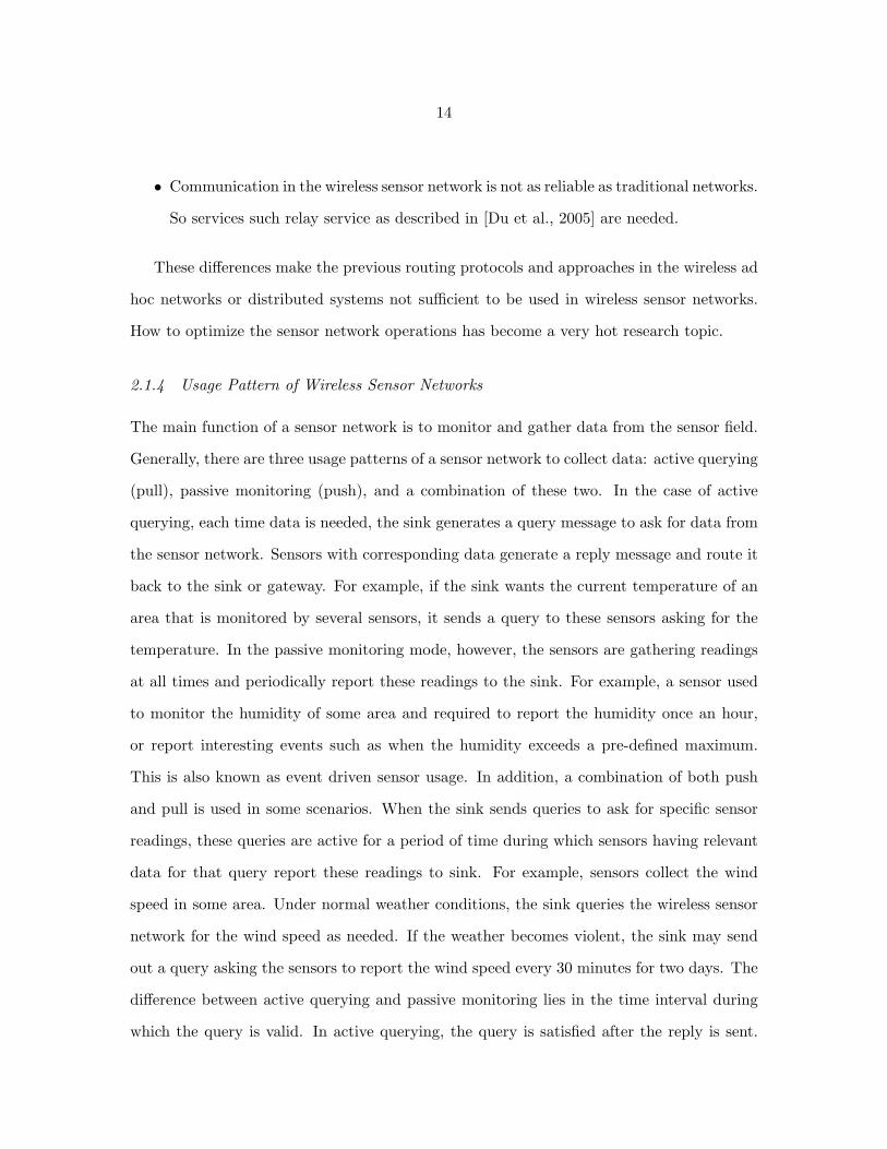
2.1.4 Usage Pattern of Wireless Sensor Networks

The main function of a sensor network is to monitor and gather data from the sensor field.

Generally, there are three usage patterns of a sensor network to collect data: active querying

(pull), passive monitoring (push), and a combination of these two. In the case of active

querying, each time data is needed, the sink generates a query message to ask for data from

the sensor network. Sensors with corresponding data generate a reply message and route it

back to the sink or gateway. For example, if the sink wants the current temperature of an

area that is monitored by several sensors, it sends a query to these sensors asking for the

temperature. In the passive monitoring mode, however, the sensors are gathering readings

at all times and periodically report these readings to the sink. For example, a sensor used

to monitor the humidity of some area and required to report the humidity once an hour,

or report interesting events such as when the humidity exceeds a pre-defined maximum.

This is also known as event driven sensor usage. In addition, a combination of both push

and pull is used in some scenarios. When the sink sends queries to ask for specific sensor

readings, these queries are active for a period of time during which sensors having relevant

data for that query report these readings to sink. For example, sensors collect the wind

speed in some area. Under normal weather conditions, the sink queries the wireless sensor

network for the wind speed as needed. If the weather becomes violent, the sink may send

out a query asking the sensors to report the wind speed every 30 minutes for two days. The

difference between active querying and passive monitoring lies in the time interval during

which the query is valid. In active querying, the query is satisfied after the reply is sent.

15

On the other hand, the query will last for a long time in passive monitoring during which

time reply messages are sent repeatedly. With hybrid monitoring, the query duration varies;

sometimes the query lasts a long time and other times it quickly becomes invalid.

2.1.5 Communication Models in Wireless Sensor Networks

The main usage of wireless sensor network is to collet the data from the monitoring field.

Usually, there are four communication models used in wireless sensor network to collect data.

We can classify the communication models in sensor networks into four types: Unicast, Area

Multicast, Area-Anycast, and Broadcast. These four communication models are abstracted

to fit the characteristics of the data source. The difference among the four communication

models lies in the granularity of the area of the data source. In the unicast model, the

data source of a query is an individual sensor, so the communication is just point-to-point

communication between the sink and one sensor, e.g., the query is delivered from the sink

to the sensor and the data is collected in the reverse way. Area multicast is used when

application is interested in the data from a certain area, so it routes the query to all sensors

in a certain area, and then all the sensors in the area generate a reply message to the sink.

Alternately, area-anycast is also interested in readings in a certain area, so it routes the

query to a specific area and at least one sensor in this area sends a reply message to the

sink. Finally, in the case of broadcast, the query message is routed to every sensor in the

network, and all sensors with corresponding data return a reply to the sink. These four

communication models can be used in the usage patterns described in previous subsection.

2.1.6 Two Query Protocols

In the wireless sensor network, there are two major query protocols as depicted in [Sha

et al., 2006b]. These two query protocols are named direct query denoted as Traditional

and indirect query denoted as IQ. In direct query protocol, the query is directly sent from

sink to the sensors that may have the corresponding data, and the sensors that do have the

16

corresponding data will send the data back to sink. While this approach has a problem of

load imbalance, so IQ is proposed to balance the load. The basic idea of IQ can be described

as the following three steps. First, the data sink randomly selects a sensor as the query

delegate and forwards the query to the delegate. Second, the delegate gets the query and

conducts the query processing on behalf of the data sink, and then aggregates the replies.

Third, the delegate sends the aggregated reply back to the data sink. Comparing with the

traditional query model, two extra steps, query forwarding and query replying, are added

in the IQ protocol. Moreover, for point-to-point communication pattern (as Unicast), the

performance of IQ is the same as that of the traditional model by choosing the sink as

the delegate, but for point to area multicast (and broadcast), such as direct diffusion and

flooding (broadcast) based approaches, it will be very helpful.

2.1.7 Routing Protocols

In traditional sensing systems, routing protocol has been extensively explored. Among them

we lists several typical routing algorithms as follows.

Greedy geographic routing. GEAR [Yu et al., 2002] and GPSR [Karp and Kung,

2000] are two greedy geographic routing protocols that are close to our work. Both of them

have not consider the global information and the local hole information. Especially, GPSR

is a purely greedy geographic routing protocol. Furthermore, the derived planer graph in

GPSR is much sparser than the original one, and the traffic concentrate on the perimeter

of the sparser planar graph in the perimeter node using GPSR make node on planar graph

depleted quickly. Thus, they are not so load balanced and fault tolerant.

Fault tolerant routing. A novel general routing protocol called WEAR [Sha et al.,

2006a] is then proposed by taking into consideration four factors that affect the routing

policy, namely the distance to the destination, the energy level of the sensor, the global

location information, and the local hole information. Furthermore, to handle holes, which is

a large space without active sensors caused by fault sensors, WEAR propose a scalable, hole

17

size oblivious hole identification and maintenance protocol. Gupta and Younis propose a

fault-tolerant clustering in [Gupta and Younis, 2003]; Santi and Chessa give a fault-tolerant

approach in [Santi and Chessa, 2002]. Both of them try to recover the detected faulty

nodes, which is actually infeasible when WSN is deployed to a forbidden place. Another

fault tolerant protocol by Datta is posted in [Datta, 2003], but it is specific for a low-mobility

and single hop wireless network. On the other hand, in WEAR, sensors try to avoid routing

messages to a failed field. Other work such as fault tolerant data dissemination by Khanna

et al. [Khanna et al., 2004] uses multi-path to provide the fault tolerant, which has to keep

more system states to achieve the goal.

Information exploiting routing. Data-centric routing such as Direct Diffusion [In-

tanagonwiwat et al., 2000] use interest to build the gradient and find a reinforced path to

collect data. RUGGED [Faruque and Helmy, 2004] by Faruque and Helmy direct routing by

propagating the events information. However, all of them pervade useful information. On

the contrary, WEAR distributes harmful hole information. Similar to WEAR, GEAR tries

to learn the hole information. However, the hole information propagation is much faster

and more sufficient in WEAR than that in GEAR. Furthermore, GEAR needs to keep a

large amount of information for every destination.

2.2 Vehicular Networks

About half of the 43,000 deaths that occur each year on U.S. highways result from vehicles

leaving the road or traveling unsafely through intersections. Traffic delays waste more than

a 40-hour workweek for peak-time travelers [VII, ]. Fortunately, with the development of

micro-electronic technologies and wireless communications, it is possible to install an On-

Board-Unit (OBU), which integrates the technologies of wireless communications, micro-

sensors, embedded systems, and Global Positioning System (GPS), on vehicles. By enabling

vehicles to communicate with each other via Inter-Vehicle Communication (IVC) as well as

with roadside units via Roadside-to-Vehicle Communication (RVC), vehicular networks can

contribute to safer and more efficient roads by providing timely information to drivers

18

Rode Side Unit

DoTServer

PrivateServer

Figure 2.3: A typical authentication scenario.

and concerned authorities. After having more and more vehicles are equipped with the

communication devices, the vehicular network is becoming one of the largest ad hoc sensing

systems that exist in our daily life.

Vehicular networks can be used to collect traffic and road information from vehicles,

and deliver road services including road warning and traffic information to the users in the

vehicles. Thus, a great attention has been put into designing and implementing similar

systems in the past several years [Bishop, 2000, ITSA and DoT, 2002]. Several typical

vehicular network applications are described as follows. First, vehicular networks can be

used as traditional sensor networks with higher mobility, thus, vehicles can be used to collect

the environmental condition and send them via the inter-vehicle communication and vehicle-

to-roadside communication. In vehicular networks, we find that there are mainly two types

of data will be collected, each of which has its specific features. One is regular data which

includes normal whether conditions, normal road conditions and some information about

the vehicle itself such as location, velocity and direction. This type of data usually has

low real-time requirements, which is usually used for long-term analysis. The other type

of data is events data, which includes sudden brake, heavy traffic, car accident, hard turn,

19

wild whether conditions such as icy and froggy. These kinds of data usually has high real-

time requirements, which should also be delivered to give warning to others vehicles on the

road. Second, utilizing the collected data, vehicular networks are very helpful to improve

the safety in drive. With the inter-vehicle communication, safety warning information can

be delivered in a timely way so that the driver can response before severe damage happens.

Third, a lot of location-based service can be deployed in vehicular networks. For example,

intelligent navigation system can be designed based on the real-time traffic information

collected by the vehicular networks. Other location-based road aid service like featured

store reminding can also deployed in vehicular networks.

2.2.1 Architecture of Vehicular Networks

A vehicular network consists of a set of vehicles on the road, a set of road side unit (RSU),

and a number of remote server, as shown in Figure 2.3. Usually, the vehicles will move on the

road and collect information such as road conditions, environmental parameters or detected

events. Each vehicles acts like a mobile sensor mote with the capability of computation,

communication and sensing. RSUs are deployed along the road, acting as fixed sensor

motes, which can also capable of computation, communication and sensing. In most cases,

the RSUs are more powerful than vehicles in terms of computation and communication.

Remote servers are mostly located far away from the road and they are normally much

more powerful and have high ability in data processing. The communication happens in

several cases, including between RSUs and vehicles, among vehicles and between RSUs and

remote servers. Dedicated Short Range Communications (DSRC) is the designated wireless

protocol for a vehicular network [DSRC, ], which is used in the communication between

RSUs and vehicles as well as among vehicles. Internet based communication is exploited to

transfer data between RSUs and the remote server as well as among RSUs.

20

2.2.2 Characters of Vehicular Networks

Compared with other wireless sensor networks, vehicular networks have their special fea-

tures. First of all, vehicular networks usually include a very large amount of vehicles, but

only when these vehicles are driving on road, they are involved in the network. Further-

more, the vehicle is moving very fast on the way, thus the network is highly dynamic. As a

result, it lacks permeant relationship among vehicles and RSUs as well as among different

vehicles. Second, in such a totally distributed environment, all decisions should be made

locally based only on partial information. Moreover, some decisions have to be made in

a real-time format. Third, one major application of vehicular networks is to improve the

safety, thus safety is a big concern in vehicular networks; then, an emergency event should

be reported and confirmed by other vehicles or RSUs on time. Making an accurate real-time

decision based on partial information is a big challenge. Also, security will be considered

the vehicular network design to prevent malicious attacks. Fourth, because vehicular and

drivers are closed entangled, drivers will have big concerns to keep privacy, such as location

privacy and service usage pattern privacy. Finally, vehicles are usually installed big and

rechargeable batteries, so the energy constraints in the vehicular network is not as high as

that in the traditional sensor networks and both communication and computation are also

more powerful than the traditional sensor networks.

2.3 Healthcare Personal Area Networks

The medical system has not been able to effectively adapt to the dramatic transformation

in public health challenges; from acute to chronic and lifestyle-related illnesses . Although

acute illnesses can be treated successfully in an office or hospital, chronic illnesses comprise

the bulk of health care needs and require a very different approach. There is overwhelming

consensus that the prevention and treatment of cardiovascular disease, diabetes, hyperten-

sion, chronic pain, obesity, asthma, HIV, and many other chronic illnesses require substantial

patient self-management.

21

People need to monitor their bodies, reduce physiological arousal when stressed, increase

physical activity, and avoid or change harmful environments. Yet, there is a lack of effec-

tive and easily deployed tools for self-monitoring, and people often do these tasks poorly,

especially people at socioeconomic risk for chronic illness, such as urban minorities. That

is, people most at risk for costly chronic illnesses have the least access to self-management

tools. Based on current cognitive and behavioral change research, we are convinced that the

prevention or treatment of chronic illnesses will be greatly aided by an innovative system

that can monitor one’s body, behavior, and environment during a person’s daily life, and

then alert the person to take corrective action when health risks are identified. This goal

reflects the view of Microsoft Corporation president Bill Gates, who noted in a recent Wall

Street Journal article, “What we need is to put people at the very center of the health-care

system and put them in control of all of their health information”.

Currently, smart phones and personal assistant devices, are widely used in field research

to collect information from participants. For example, at random or pre-set times, a person

is prompted to respond to questions. Moreover, there are numerous devices available to

record physiological responses in real life, such as blood pressure and heart rate. Thus,

healthcare personal area networks are developed by utilizing those devices to help people

to monitor their body conditions and get some feedback or suggestions from healthcare

expertise.

In this dissertation, we introduce SPA, a smart phone assisted chronic illness self-

management participatory sensing system. SPA represents a general architecture of a

healthcare personal area sensing network. There are three main functions of the system.

First, it is used to collect real-time biomedical and environmental data from the participant

using sensors, which will be very useful for us to understand the possible causes of the chronic

illness. Second, the data analysis and data mining algorithms are used to find time-series

rules and the relationship between the biomedical and environmental parameters, which will

help health care professionals to design health care plans for specific participants. Third,

22

Biosensor: Heart Rate, Blood Pressure

Environmental Sensor: Sound, Light,

Temperature ...

Activity Sensor: Accelerometer

 

 

 

Bluetooth

GPS Position

Wi-Fi

3G or GPRS

Remote Server

Survey TriggeringData StorageData MiningWeb PublishingAlarm Notification

`

Figure 2.4: The architecture of the SPA system.

the system automatically triggers on-line surveys and sends out alarm notifications, largely

reducing the involvement of the health care professionals, which not only saves medical cost

but also protects the participants as early as possible. Next, we give a detailed description

of SPA system design.

2.3.1 The Architecture of the SPA System

The SPA system consists of three major parts as shown in Figure 2.4, including a body area

sensor network to collect biomedical and environmental data, a remote server to store and

analyze data, and a group of health care professionals to check records and give health care

suggestions.

The body area sensor network includes a smart phone, a set of biosensors and a set of

environmental sensors. The smart phone works as a base station for the body area sensor

network, which can not only receive and temporarily store sensed data but also work as a

router to communicate with the remote server. Moreover, the smart phone is also equipped

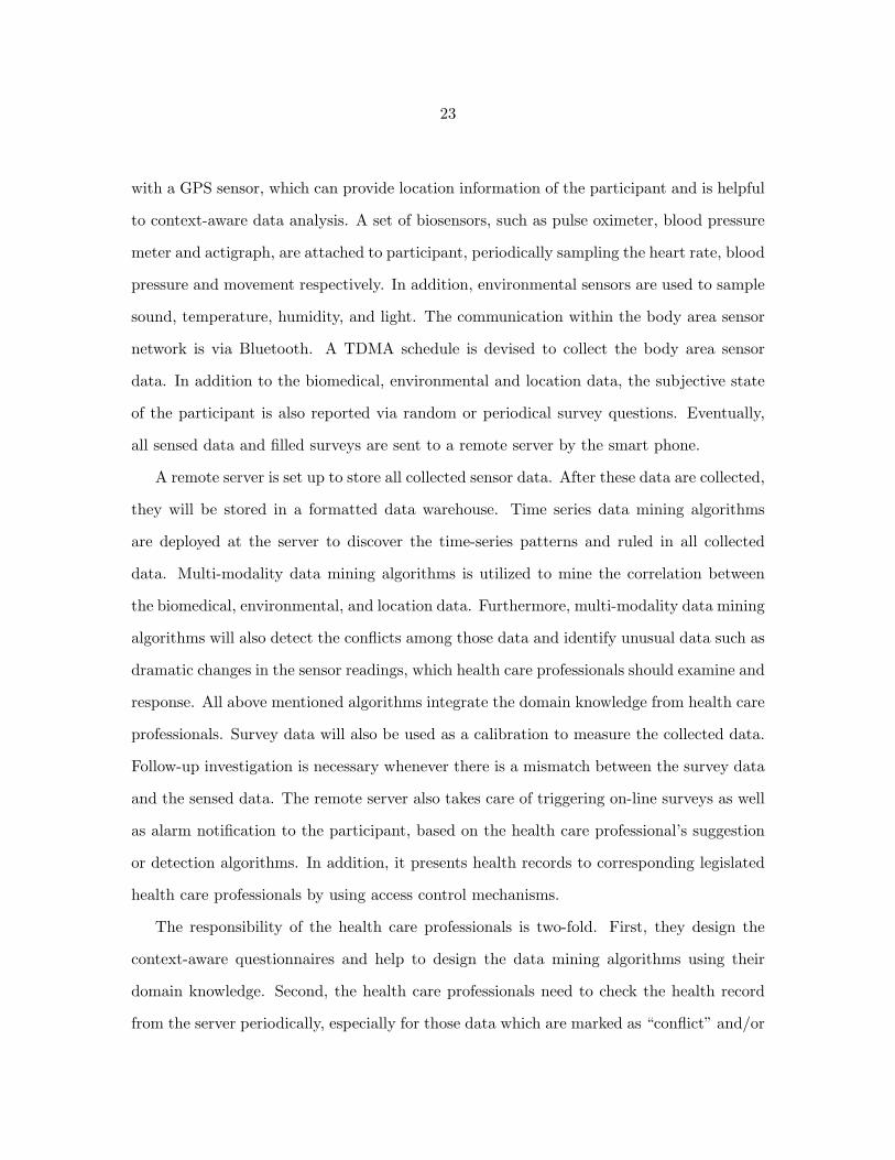
23

with a GPS sensor, which can provide location information of the participant and is helpful

to context-aware data analysis. A set of biosensors, such as pulse oximeter, blood pressure

meter and actigraph, are attached to participant, periodically sampling the heart rate, blood

pressure and movement respectively. In addition, environmental sensors are used to sample

sound, temperature, humidity, and light. The communication within the body area sensor

network is via Bluetooth. A TDMA schedule is devised to collect the body area sensor

data. In addition to the biomedical, environmental and location data, the subjective state

of the participant is also reported via random or periodical survey questions. Eventually,

all sensed data and filled surveys are sent to a remote server by the smart phone.

A remote server is set up to store all collected sensor data. After these data are collected,

they will be stored in a formatted data warehouse. Time series data mining algorithms

are deployed at the server to discover the time-series patterns and ruled in all collected

data. Multi-modality data mining algorithms is utilized to mine the correlation between

the biomedical, environmental, and location data. Furthermore, multi-modality data mining

algorithms will also detect the conflicts among those data and identify unusual data such as

dramatic changes in the sensor readings, which health care professionals should examine and

response. All above mentioned algorithms integrate the domain knowledge from health care

professionals. Survey data will also be used as a calibration to measure the collected data.

Follow-up investigation is necessary whenever there is a mismatch between the survey data

and the sensed data. The remote server also takes care of triggering on-line surveys as well

as alarm notification to the participant, based on the health care professional’s suggestion

or detection algorithms. In addition, it presents health records to corresponding legislated

health care professionals by using access control mechanisms.

The responsibility of the health care professionals is two-fold. First, they design the

context-aware questionnaires and help to design the data mining algorithms using their

domain knowledge. Second, the health care professionals need to check the health record

from the server periodically, especially for those data which are marked as “conflict” and/or

24

“unusual data”. Follow-up suggestions are expected after the health care professionals

examine the health record. In our design, trying to reduce the involvement of the health

care professionals as much as possible, most surveys and alert notifications, after they are

designed, will be automatically generated by the server, based on the predetermined rules

and the value of the currently received data. Only when it is in urgent cases will health

care professionals be involved to provide support to the system.

The above mentioned three major parts in the SPA system are connected by using a

variety of communication protocols. Within the body area network, Bluetooth is adopted

to connect the sensors and the smart phone. A TDMA based schedule is designed for

the smart phone to collect data from the sensors. If the smart phone is not available

during the scheduled time, the sensors will store the data locally and temporarily. Thus,

loose synchronization is enough between the smart phone and the sensors. Aggregation

algorithms are applied when the volume of the data exceed the size of available storage.

The communications between the smart phone and the server can be either WLAN or

cellular network based on the network availability and energy concerns. The health care

professionals usually access the health record via Internet. The data flow from the sensors

to the smart phone, and eventually, data arrive at the remote server. The feedbacks and

the questionnaires are initialized by the health care professionals, mostly automatically

triggered by the system, and eventually delivered to participants.

2.3.2 Characters of the Healthcare Personal Area Networks

Compared with traditional sensing systems and vehicular networks, healthcare personal

area sensing networks have several special features. First, the system is more heterogenous

than traditional sensing systems. For example, multiple communication radios may be

exploited in the communication. Bluetooth, UWB, and Zigbee protocol may be utilized the

communicate the body area sensors and the smart phone or PDAs. Wifi or cellular networks

may be used to transfer the information from PDAs to a centralized server. A variant

25

of sensing devices can be used to sense personal biophysical conditions, including blood

pressure, heart rate, movement and temperature. Second, The data collected by biosensors

and location information are sensitive personal information. Usually, participants are not

willing to release such data to the public. Thus, privacy is one of the most important design

issues in this type of sensing system. Third, the sensing parameters are more context-aware

than sensing parameters in traditional sensing systems. From this perspective, more rich

data will be collected. Forth, the communication and data collection in healthcare personal

area networks will not take the same strategy as those in most traditional sensor networks.

Collected data will be sent mostly in one-hop, but not using multi-hop routing protocols.

26

CHAPTER 3

RELATED WORK

Having introduced the basic structure and features of the wireless sensor network. In

the rest of this chapter, we will introduce some relate work to our design. These previous

efforts include the energy efficiency design, the definition for the lifetime of wireless sensor

networks, data consistency models, adaptive protocol design, data quality management, and

MAC protocol respectively.

3.1 Related Definition of Lifetime of Wireless Sensor Network

Energy-efficient routing protocols and optimizations to maximize the lifetime of sensor net-

works have been widely studied in the literature [Akkaya and Younis, 2003]; however, few

of the previous efforts have been done to formally model the lifetime of the sensor network.

To this end, our work is the first step towards this direction.

In several previous work, the lifetime of the sensor network is defined as the time for

the first node to run out of power such as in [Chang and Tassiulas, 2000,Heinzelman et al.,

2000,Kalpakis et al., 2002,Kang and Poovendran, 2003] or a certain percentage of network

nodes to run out of power as in [Duarte-Melo and Liu, 2003,Xu et al., 2001a]. We think

that these definitions of the lifetime of the sensor network are not satisfactory. The former

is too pessimistic since when only one node fails the rest of nodes can still provide the whole

sensor network appropriate functionality. While the latter does not consider the different

importance of the sensors in the sensor network, as shown in Section 7.2 the failure sensors

in different location will have different influence to the whole sensor network.

In the work of [Bhardwaj and Chandrakasan, 2002,Bhardwaj et al., 2001,Blough and

Santi, 2002,Mhatre et al., 2004], the lifetime of the sensor network is defined as the time

27

when the sensor network first losts connectivity or coverage. The rationale of their defini-

tion is based on the functionality of the sensor network, which is similar to our definition.

However the way to detect the termination of the sensor network is different. Blough and

Santi [Blough and Santi, 2002] define it by checking the connectivity of a graph; Mhatre

et al. use a connectivity and coverage model to describe it; while we define it as the time

when the remaining lifetime of the whole sensor network starts to keep constant as losing

connectivity or the sensor network loses coverage.

Xue and Ganz study the lifetime of a large scale sensor network in [Xue and Ganz,

2004]. They explore the relationship between the lifetime of a sensor network with the

network density, transmission schemes and maximum transmission range. Their work is

based on a general cluster-based model, and does not consider the importance of different

sensors. They also aim to explore the fundamental limits of network lifetime. Compared

with their work, our model is more general which can be used not only for cluster-based

model. Furthermore, because we take more factors into consideration in our model, our

model is more useful and flexible, in which the lifetime is calculated according to the really

energy consumption.

Bhardwaj et al. define upper bounds on the lifetime of the sensor network in [Bhardwaj

and Chandrakasan, 2002, Bhardwaj et al., 2001]. They explore the fundamental limits of

data gathering lifetime that previous strategies strive to increase. One of their motivations

is to calibrate the performance of collaborative strategies and protocols, but they just give

out an upper bound of the lifetime rather than the actually lifetime model for different

strategies. Besides, our model can also guide the design of the low-level protocols.

Another recent work has been done also aim to derive the upper bound of the lifetime of

a sensor network in [Zhang and Hou, 2004]. The authors want to explore the fundamental

limits of sensor network lifetime that all algorithms can possibly achieve. Compared with

their work, our model is aiming to develop models for both sensor system designer and

application scientist, and we focus on calculating the more accurate lifetime of a sensor

28

network according to different underlayer routing or query protocols. In both our work, we

consider the coverage and connectivity of the sensor network.

Duarte-Melo and Liu provide a mathematical formulation to estimate the average life-

time of a sensor network in [Duarte-Melo and Liu, 2003]. Their work aims to estimate the

average lifetime of the sensor network rather than to provide a general model that can be

used to measure different protocols. Our model can be used to model the lifetime of the

sensor network using different communication patterns, which is more general. In their

later work, they give a modeling frame for computing lifetime of a sensor network. Their

approach is to maximize the functional lifetime of a sensor network and get the value of it

based on the solution of a fluid-flow model. While our goal of this dissertation is to provide

a general model for lifetime of sensor network. Besides, the calculation of their lifetime still

need a lot of calculation. While our model can be easily calculated based on the centralized

algorithms.

Similar to [Duarte-Melo and Liu, 2003], several other efforts such as in [Kalpakis et al.,

2002, Kang and Poovendran, 2003, Sadagopan et al., 2003, Mhatre et al., 2004, Shah and

Rabaey, 2002] have been done to maximize the lifetime of sensor network. Whereas almost

all their work take it as an optimization problem and build a linear programming model, then

find an algorithm or a protocol to achieve the maximum lifetime, so that these approaches

are always closely related to the routing protocols, rather than giving a general model for

the lifetime of sensor network. Besides, most of them ignore the load imbalance problem.

Even though some of them do notice the problem, they only balance the load at the routing

level.

Energy-aware routing [Shah and Rabaey, 2002] is proposed by Shah et al. using a set

of sub-optimal paths to increase the lifetime of the network. This approach uses one of

multiple paths with a certain probability to increase the lifetime of the whole network.

Another similar approach is proposed in [Dai and Han, 2003], which constructs a load

balance tree in the sensor networks with load balance to different branches. Their work

29

balances the load of each data path so that extend the lifetime of sensor networks. They

do not provide a formal model for the lifetime.

3.2 Related Sensing Data Analysis

SenseWeb [SenseWeb, ] has provided a venue for people to publish their data, but we

have not seen any analysis yet. Our next step will use more data set from SenseWeb.

Data aggregation is an important way to reduce the volume of the collected data. A few

data aggregation approaches have been proposed. These approaches make use of cluster

based structures [Heinzelman et al., 2002] or tree based structures [Ding et al., 2003,

Goel and Estrin, 2003, Intanagonwiwat et al., 2002,Luo et al., 2005,Zhang and Cao, 2004].

Considering applications which require some aggregate form of sensed data with precision

guarantees, Tang and Xu propose to differentiate the precisions of data collected from

different sensor nodes to balance their energy consumption [Tang and Xu, 2006]. Their

approach is to partition the precision constraint of data aggregation and to allocate error

bounds to individual sensor nodes in a coordinated fashion.

As the tradeoff between data quality and energy consumption has been considered in a

few data aggregation protocols, adaptive sampling provides another way to minimize energy

consumption while maintaining high accuracy of data. Essentially, n adaptive sampling

design, the sensor nodes which send out data and the rate of data transmission are selected

adaptively.

Adaptive sampling has been proposed to match sampling rate to the properties of envi-

ronment, sensor networks and data stream. Jain and Chang propose an adaptive sampling

approach called backcasting [Jain and Chang, 2004], which first makes an initial correlation

estimate by having a small subset of the wireless sensors communicate their information to a

fusion center, then selectively activates additional sensors in order to achieve a target error

level. Gedik and Liu proposed a similar way of data collection, selective sampling [Gedik

and Liu, 2005]. Their selective sampling algorithm uses a dynamically changing subset of

30

nodes as samplers to predict the values of non-sampler nodes through probabilistic mod-

els. This approach assigns nodes with close readings to the same clusters, and prediction

model is used to minimize the number of messages used to extract data from the network.

Although many approaches have been proposed to reduce energy while maintaining data

quality, there exists rare study on the pattern of raw data collected by sensor nodes in the

real world. In addition, most studies adopt the way of simulation, To examine how well

those approaches fit our real world, and to inspire new approaches, it’s necessary to study

the raw data carefully under systematic guidelines, whereas, our quality-oriented sensing

data analysis gives a chance to take a fresh look at how the data behaves. We made use

of reappearance pattern, empirical distribution, trend comparison, multimodality analysis

and spatial correlation to present a clear view of the sensing data, and many interesting

facts are discovered. These findings, in turn, enhance our understanding of the reality of

today’s wireless sensor networks. The idea is to combine the data coming from different

sensor nodes, eliminating redundancy, minimizing the number of transmissions and thus

saving energy. We are the first that formally define a set of consistency models for WSNs.

We also design and implement an adaptive, lazy, energy efficient data collection protocol to

improve data quality and save energy.

3.3 Related Energy Efficiency Design

Energy efficiency is always one of the major goals in the design of WSN. Energy efficient

protocols have been explored for a long time. Previous work expects to achieve the goal of

energy efficiency by designing energy efficient query protocols [Sha and Shi, 2006a], rout-

ing protocols, such as [Braginsky and Estrin, 2002,Chang and Tassiulas, 2000,Hamdaoui

and Ramanathan, 2006,He et al., 2003,Heinzelman et al., 1999,Heinzelman et al., 2000, In-

tanagonwiwat et al., 2000,Kalpakis et al., 2002,Lindsey et al., 2002,Lindsey et al., 2001,Mad-

den et al., 2002,Manjeshwar and Agrawal, 2001,Manjeshwar and Agrawal, 2002,Sadagopan

et al., 2003, Schurgers and Srivastava, 2001, Seada et al., 2004, Sha and Shi, 2004, Sha and

Shi, 2005,Shah and Rabaey, 2002,Xu et al., 2001b,Yao and Gehrke, 2002], energy efficient

31

MAC protocols like [Polastre et al., 2004,Shih et al., 2001,Ye et al., 2002,Woo and Culler,

2001], energy efficient clustering [Younis and Fahmy, 2004], duty cycle management [Das-

gupta et al., 2003, Younis et al., 2002,Younis and Fahmy, 2004], sensor network topology

management [Gupta et al., 2008], and other energy efficient approaches [Sadagopan and

Krishnamachari, 2004]. However, these approaches mainly focus on finding some energy

efficient path, designing better turn on/off schedules, forming energy efficient clusters, and

so on, but none of them has examined the energy efficiency from the view of the data it-

self, i.e., to adapt the data sampling rate to the data dynamics and keep lazy when data

consistency is maintained. Thus, we are first to design an energy-efficient protocol from the

prospective of data consistency.

Aggregation is one of the most common technologies used in wireless sensor networks to

save energy. Aggregation structures such as TAG [Dasgupta et al., 2003, Intanagonwiwat

et al., 2002, Madden et al., 2002] are designed to aggregate the message. Another work

from [Shrivastava et al., 2004] propose new aggregation scheme that significantly extends

the class of queries that can be answered using sensor networks. We also use aggregation

in our protocol, and we not only take advantage of the previous aggregation techniques but

also try to combine several pieces of data together.

Load balanced protocols are designed in different layer of sensor systems to save energy

and extend the lifetime of wireless sensor networks. Dai and Han in [Dai and Han, 2003]

construct a load balanced tree in the sensor networks to make the load evenly distribute to

different branches of the routing tree. Indirectly Query [Sha et al., 2006b] is proposed to

balance the load at query layer so that it extends the lifetime of WSN a lot. At the higher

level, several researchers have been proposed to balance the load of sensors by rotating

their functionality, including coordinators in topology management [Chen et al., 2001],

rotation of grid zone headers in GAF routing [Xu et al., 2001a], rotating cluster headers in

hierarchical protocols [Heinzelman et al., 2000], and switching among multi-paths during

routing [Ganesan et al., 2002].

32

Energy aware routing is also used to save energy and extend the lifetime of wireless

sensor networks. Shah and Rabaey propose an energy aware protocol [Shah and Rabaey,

2002]. They keep using a set of good paths instead of just finding a single optimal path and

use different path at different time with some probability depending on the energy metric.

Younis et al. [Younis et al., 2002] design a energy-aware routing for cluster-based sensor

network. In their approach, the gateway in each cluster applies energy-aware metrics to

manage the topology adjustment and routing setup, but the cluster based scheme is argued

to be energy inefficient. GEAR [Xu et al., 2001a] and WEAR [Sha et al., 2006a] are both

used energy aware approach to balance the load to different sensors so that they extend the

lifetime of WSN significantly.

Duty cycle management and sensor network topology management are two other ap-

proaches to achieve the goal of energy efficiency. In [Dasgupta et al., 2003, Younis et al.,

2002,Younis and Fahmy, 2004], the authors try to design an on/off schedule for sensors so

that they can save energy by making sensors sleep as much as possible. However, we argue

that the design of duty cycle schedule in sensing systems should be integrated with the

data quality management by taking data consistency into consideration. Gupta proposes

a topology management mechanism in sensor networks to save energy [Gupta et al., 2008].

The basic idea of this approach is to take advantage of the redundant sensors. To be specific,

they pick up a set of sensors from the sensor network and make sure that this set of sensors

are sufficient to reconstruct data for the entire sensor networks. This approach can save

energy but it also introduce load imbalance, and it cannot satisfy some applications that

require a certain level of data redundant. In general, our data quality management scheme

complements this kind of approaches very well by considering both energy efficiency and

data quality.

3.4 Related Data Consistency Models

Data consistency is a classical problem in computer architecture, distributed systems,

database, and collaborative systems. Interesting readers please refer to [Peterson and Davie,

33

2003,Ramakrishnan, 1998,Tanenbaum and van Steen, 2002]. A lot of consistency models,

such as strict consistency, causal consistency, weak consistency, eventual consistency, have

been proposed in the research of these fields. However, these models are usually not ap-

plicable in WSN. For example, these models are working on how to keep consistency for

several duplicated data in the a distributed environment. However, in this dissertation, we

do not consider the problem of duplicated data sampled from different sensors but the data

consistency between the real time in the data field and the received data at the sink. Thus,

these models are not applicable in our scenario.

The work form Yu and Vahdat [Yu and Vahdat, 2000] explores the semantic space

between traditional strong and optimistic consistency models for replicated services. They

propose an important class of applications can tolerate relaxed consistency, but benefit

from bounding the maximum rate of inconsistent access in an application-specific manner.

Thus, they develop a set of metrics to capture the consistency spectrum. Similar to us,

they also consider the application requirements to the data in the data consistency models.

However, their models are still for different replicas and so that they are suitable for using

in traditional distributed system instead of being applied in the field of wireless sensor

networks.

Ramamritham et al. propose an idea to maintain the coherency of dynamics data in

the dynamics web monitoring application [Shah et al., 2003]. They address the problem of

maintaining the coherency of dynamic data items in a network of repositories using filters.

In their follow-up work in [Gupta et al., 2005], they model the dynamics of the data items.

Based on the dynamics of data, they adapt the data refresh time to deliver query results

with the desired coherency. Their work is similar to ours; for example, both of their work

and our work want to model the data dynamics and design adaptive protocol to deliver

data; however, their work is to collect data from the web, and our work is to collect data

in wireless sensor network, which is more resource constraint. Moreover, we have different

34

goal in data operations from theirs so that we use a different protocol and different models,

and our model for data consistency is more general than theirs.

Lu et al. propose a spatiotemporal query service that allows mobile users to period-

ically gather information from their surrounding areas through a wireless sensor network

in [Chipara et al., 2005, Lu et al., 2005], and their goal is to provide a service to enable

mobile users to periodically gather information and meet the spatiotemporal performance

constraints. They propose spatial constraints and temporal constraints to the query and

collected data, but in their work they propose neither data consistency models, nor adaptive

protocols. Furthermore, their work is most useful in a system with high real-time require-

ments, while our work defines general consistency model which can be applied in different

applications with variant data consistency requirements. However, their work compliments

to our effort very well, i.e., we can integrate their approach with our data consistency mod-

els by using their service in the scheduling of our protocol. Thus, as far as we know, this is

the first model to define the data consistency in WSN.

Information assurance is proposed in [Deb et al., 2003]. Their work intends to dissem-

inate different information at different assurance levels to the end-user so that they can

deliver critical information with high assurance albeit potentially at a higher cost, while

saving energy by delivering less important information at a lower assurance level. They

propose a scheme for information delivery at a desired reliability using hop-by-hop broad-

cast, based on which they can attain given desired end-to-end reliability. We share the

similar goals with their work, i.e., we want to guarantee the end-to-end data consistency

and treat different data with different priority according to their application specific con-

sistency requirements; however, they neither abstract the application requirements to the

different information nor propose consistency model. Moreover, they use different protocol

to collect data in an energy efficient way.

35

3.5 Related Adaptive Design in Wireless Sensor Networks

Adaptive approaches, which usually fit the changes of the environment or the different

requirements of the applications, are always attractive in system design. Several adaptive

protocols including [Cerpa and Estrin, 2002, He et al., 2002, Heinzelman et al., 1999, Lin

and Gerla, 1997,Mainland et al., 2005] are proposed in literature. However, these protocols

mostly focus on the cluster formation, communication patten selection, and duty cycle

designing. None of them intends to adapt the data sampling rate according to the data

dynamics.

A family of adaptive protocols called SPIN are proposed by Heinzelman et al. in [Heinzel-

man et al., 1999] to efficiently disseminate information in wireless sensor networks. They

intend to develop a resource aware and resource adaptive sensor networks, e.g., when the

sensors’ energy is approaching a low-energy threshold, it adapts by reducing its participa-

tion in the protocol. However, we argue that making decision only based on the current

available resource is not enough to optimize the performance of the application specific

sensor networks, the requirements from application should be considered as well.

ASCENT [Cerpa and Estrin, 2002] is proposed to make sensors coordinate to exploit the

redundancy provided by high density, so as to extend overall system lifetime. In ASCENT,

each node assesses its connectivity and adapts its participation in the multi-hop network

topology based on the measured operating region. Their goal is to adapt the sensor to a

wide variety of environment dynamics and terrain conditions by managing the duty cycle.

Thus, they are interested in different problems from us. As a result, they intend to ex-

tend the lifetime of wireless sensor network by topology control instead of considering data

consistency.

In [He et al., 2002] He et al. propose a novel aggregation scheme that adaptively performs

application independent data aggregation in a time sensitive manner. Their work isolates

aggregation decisions into a module between the network and the data link layer. The

basic idea of their approach is taking advantage of queueing delay and the broadcast nature

36

of wireless communication to concatenate network units into an aggregate. They design

a feedback based adaptive component to make on-line decision on how many packets to

aggregate and when to invoke such aggregation based on local current network conditions.

Compared with our work, the adaption happens after the data is collected, while in our

approach the adaption happens during sampling data. So we can integrate their work and

our work together and take advantage of both adaption.

A recent paper [Mainland et al., 2005] from Mainland et al. uses adaptive approach to

allocate the resource for sensor networks. They model the sensor as a self-interested agent

and use price to tune the behavior of each sensor. Their goal is to maximize the profit of

each sensors under the constraints of energy budget. In their design, they can also adapt

the sampling rate to the data dynamics based on the current energy budget. However, they

neither propose a formal model for data dynamics nor consider data consistency in their

adaptive approach. Thus their approach is not from the view of the data themselves, but

from the view of every sensor’s profit.

Several techniques on adaptive sampling rate has been proposed in the database field,

these techniques share the same goal of our adaptive protocol. Jain and Chang propose

an adaptive sampling approach for WSN [Jain and Chang, 2004]. They employ a Kalman-

Filter (KF) based estimation technique and the sensor uses the KF estimation error to adapt

the sampling rate. Their approach is different from our approach in that it has to store

more data. Moreover Kalman-Filter has matrix operation so that it is much more com-

puting intensive. Marbini and Sacks [Marbini and Sacks, 2003] propose a similar approach

to adapt the sampling rate as ours, however they do not model the data dynamics and

require an internal model, which is usually difficult to find, to compare the sampled data.

TinyDB [Madden et al., 2005] also adapts the sampling rate based on current network load

conditions, but not based on the data dynamics in the data field. Their work complements

our work very well. More work on sampling rate adaption should be done by considering the

network load condition and the data feature such as data dynamics and priorities together.

37

3.6 Related Data management in Wireless Sensor Networks

Data management has been extensively explored in previous researches. Li et al. use a

feedback-driven model-based-prediction approach to manage sensed data [Li et al., 2006],

which shares similar idea with us. Their work makes a tradeoff between the storage cost

and the communication cost; however, they do not provide a general consistency model like

us to evaluate data quality, nor do they dynamically adapt the sampling rate to improve

data quality.

Trappe et al propose MIAMI [Trappe et al., 2005], methods and infrastructure for the

assurance of measurement information, to handle the attacks on the process of measurement

(PoM attack). They propose a framework based on the development of the PoM monitors,

which is responsible for preventing corrupted measurement data. Their framework shares

the same goal as u; however, they have not formally define formal consistency models.

Furthermore, their data quality management is not a feedback-based control. Instead,

Deb et al design an information assurance protocol to disseminate different information at

different assurance levels by hop-to-hop protocols [Deb et al., 2003], which has a similar

goal as our priority differentiated data collection protocol.

Quality aware sensing architecture [Lazaridis et al., 2004]is proposed by Lazaridis et al

as a scalable data management solution for wireless sensor network applications. They also

propose some sophistic compression and prediction algorithms [Lazaridis and Mehrotra,

2003] to manage the volume of the delivered data. They consider data quality from the

perspective of timeliness and data accuracy, which is similar as our perspective, but they

do not give formal models to describe timeliness and data accuracy. Moreover, they do not

distinguish individual data and streaming data. In addition, their approach is more suitable

to be used in traditional sensing systems, and they do not detect and filter deceptive data

in their architecture. Thus, we believe that their approach is not sufficient to manage the

quality of the collected data in sensing systems.

38

Another work [Larkey et al., 2006] has been done to assure the quality of collected sens-

ing data in an environmental application, by detect measurement errors and infer missing

readings. The basic idea of their approach is to take advantage of the spatialtemporal coher-

ence of the sensing data in environmental applications, and estimate distributions to model

the data, so this is not a general framework to manage data quality in sensing systems.

Confidence-based data management for personal area sensor networks [Tatbul et al., 2004]

is proposed to achieve collecting high quality data with a certain confidence. The basic idea

is to take redundancy and other factors in to consideration in data value estimation. This

is not a general framework and it only works for personal area sensing systems.

Filters are also used to manage data by reducing the size of the data stream. Work

by Olston et al. uses an adaptive filter to reduce the load of continuous query. Their

work focuses on the adaptive bound width adjustment to the filter so that their results

are helpful to analyze our lazy approach, but they have not modeled the data consistency

and considered adapting sample rate. Sharaf et al. study the trade off between the energy

efficiency and quality of data aggregation in [Sharaf et al., 2004]. They impose a hierarchy

of output filters on WSN to reduce the size of the transmitted data. Data prioritization

in TinyDB [Madden et al., 2005] chooses the most important samples to deliver according

to the user-specified prioritization function, which is not as general as our work on data

consistency and data dynamics. Furthermore, none of protocol related work has proposed

model for data consistency, but we explore a whole issue related to data consistency and

data dynamics, and our system design is a revision based on these models.

3.7 Related MAC protocols in Wireless Sensor Networks

Previous MAC protocols can be classified into two types, contention-based and reservation-

based. IEEE 802.11 DCF [IEEE802.11, 1999] is a contention-based protocol, which builds

on MACAW [Bharghavan et al., 1994]. The basic idea of these protocols is for a sender

to transmit a request-to-send (RTS) that the receiver acknowledges with a clear-to-send

(CTS).If the RTS/CTS exchange is successful, the sender is allowed to transmit one or

39

more packets. CRAM [Garces and Garcia-Luna-Aceves, 1997b] and PRMA [Goodman

et al., 1989] try to resolve RTS collisions based on auctions or tree-splitting algorithms.

B-MAC [Polastre et al., 2004], S-MAC [Ye et al., 2002] and T-MAC [Dam and Lan-

gendoen, 2003] are specially designed for WSN. B-MAC [Polastre et al., 2004] provides

interfaces for application to control the backoff time when it initializes sending packet or

when it detects collisions. S-MAC [Ye et al., 2002] and T-MAC [Dam and Langendoen,

2003] also use adaptive listening to reduce latency, and App-MAC [Du et al., 2005] uses

the contention-based protocol to report event information. In App-MAC, they design a

mechanisms to reduce collisions, e.g., filtering out some events with specified priority and

some motes of specified types. They also design the CS assignment algorithms and the

distributed CS competing algorithm to reduce collisions and save energy. Finally, variable

length event data is considered in the design.

TDMA [Arisha et al., 2002] is a reservation-based protocol. In TDMA, a time pe-

riod is divided into frames that provide each node with a transmission slot over which it

can transmit data without collisions. NAMA [Bao and J.J.Garcia-Luna-Aceves, 2001] and

TRAMA [Rajendran et al., 2003] are based on a distributed contention resolution algorithm

that operates at each node based on the list of direct contenders and indirect interferences.

They introduce energy-efficient collision-free channel access in WSN. GAMA-PS [Muir and

Garcia-Luna-Aceves, 1998] and CRAMA-NTG [Garces and Garcia-Luna-Aceves, 1997a] use

dynamic reservation to build a transmission schedule. IEEE 802.15.4 [IEEE802.15.4/D18,

2003] (Zigbee) designs a superframe structure, which combines an active part and an op-

tional inactive part. The active part is further divided into a contention access period (CAP)

and an optional contention free period (CFP).

3.8 Related Deceptive Data Detection Protocols

A previous effort that is close to our idea is presented to detect and diagnose data inconsis-

tency failure in wireless sensor networks [Ssu et al., 2006]. The basic idea of their approach is

to build node-disjoint path and use majority voting to detect inconsistency among collected

40

data; however, in their work, they neither define data inconsistency models, nor propose a

general framework for sensing systems.

In traditional systems, outlier detection problems have been explored. Three funda-

mental approaches have been proposed to detect outliers [Hodge and Austin, 2004]. First,

unsupervised clustering techniques are used to determine the outliers with no prior knowl-

edge of the data. They assume that errors or faults are separated from normal data and will

thus appear as outliers. The basic idea is to classify data into different clusters and detect

the data outside of the cluster as outliers. We can take advantage of those algorithms in

our protocol. The other approach is called supervised classification, in which they model

both normality and abnormality. If new data is classified to abnormal area, it will be an

outlier. Those kinds of approaches require pre-knowledge so that they are not applicable

in some highly dynamic and unpredictable environment. Another approach is a mixture of

the previous two. It models only normality and a few cases abnormality.

A spatial outlier detection approach is proposed in [Shekhar et al., 2003]. They first

formally model the problem of spatial outlier detection problem, and then they use a set

of neighborhood aggregation function and distributive aggregation function to detect the

outliers. Those aggregation functions can be used in our system as well. Adam, Janeja and

Atluti design an algorithm to detect anomalies based on neighborhood information [Adam

et al., 2004]. They explore both spatial and semantic relationship among the objects taking

into consideration the underlying spatial process and the features of these spatial differen-

tiated objects. Thus, they generate a set of both micro and macro neighborhoods, based

on which outliers are detected. Bayesian network is a common used approach to classify

sensor nodes according to the spatio-temporal correlations between those sensor nodes. For

example, Bayesian belief networks are used in outlier detection [Janakiram et al., 2006].

A set of sensing data cleaning approaches have been proposed. Elnahrawy and Nath

propose an approach for modeling and online learning of spatio-temporal correlations in

sensing systems to detect and filter noise data [Elnahrawy and Nath, 2003]. This work shares

41

the similar goal with ours, however, our approach is different from theirs by leveraging the

consistency-driven concept and data dynamics for deceptive data detection and filtering.

Their approach of outliers discovery complements our approach very well, and could be

integrated into our system. A weighted moving average-based approach is proposed to

clean sensor data [Zhuang et al., 2007]. The basic idea is to average the temporal-spatial

data in an efficiency way, and detect noisy data based on the calculated average. This

idea is very similar to the role-based deceptive data detection in our framework, but their

approach is good to work in a relatively low dynamic environment while our approach can

work in a highly dynamic environment in that we define importance of roles in different

ways than them. Furthermore, our approach can take advantage of physical features in the

physical system so that our approach can reach a confirmation in a fast and confident way.

Ye and et al propose to mechanism to statistically En-route filter injected false data [Ye

et al., 2004,Ye et al., 2005]. They assume an event will be detected by multiple sensors and

rely on the collective decisions of multiple sensors for false report detection. This approach

is a security based approach and it does not really check the value of the collected data, in

other words, this approach works at the event level but not at single data level. Declarative

support for sensor data cleaning [Jeffery et al., 2006] is proposed by Jeffery et al. In their

work, the authors utilize the temporal and spatial nature of sensor data to drive many of its

cleaning process. As a result, they propose a framework named Extensible Sensor stream

Processing (ESP) to segment the cleaning process into five programmable stages. Those

stages are further integrated into a SQL-like language to clean the data. Compared with

ESP, our framework for deceptive data detection and filters are more general by considering

different types of deceptive data.

Several error correction algorithms have been presented in literature. A local, distributed

algorithm to detect measurement error and infer missing readings in environmental appli-

cations is presented in [Mukhopadhyay et al., 2004b,Mukhopadhyay et al., 2004a]. In their

work, a data distribution model is built based on the history data. Error is detected when

42

there is a mismatch between the model prediction and the sensor reading. Sensor self-

diagnostics or sensing reading calibration have been studied in [Li et al., 2007], in which

preliminary data checking, analysis and sensor diagnosis are performed on-board. They try

to build a set of rule-set based on data collected by different types of sensors and use those

rule-set to analyze sensing data. Their goal is to detect fault readings at individual sensors.

In this case, no malicious sensors are considered.

There are also deceptive data detection algorithms in vehicular networks. Probabilistic

validation of aggregated data [Picconi et al., 2006] shows a way to probabilistically detect

malicious cars that generate false aggregated information. In particular, they focus on vali-

dating speed and location information. To achieve this goal, they use a temper-proof service

in the car as a proxy to buffer and transmit data. When data is received, a probabilistic

verification is executed to validate received data. In general they adopt a security based

approach to detect malicious aggregated data. Golle et al propose a mechanism to detect

and correct malicious data in vehicular networks. They define a model of VANET, which

specifies what events or sets of events are possible. A function maps a set of events to

two values, valid and invalid. Only when the set of events are consistent, they are valid.

Otherwise, malicious data is detected. How to check the consistent among the events is

defined by a set of rules. This work shares similar ideas as our role-based deceptive data

detection protocol in VANET, but we have different ways to detect deceptive data.

From above, we find that most outlier detection and other related algorithms assume

a spatio-temporal distribution of the analyzed data, while our role-based deceptive data

detection protocol does not assume any distribution on the sensing data. On the other hand,

we propose a general framework to attack deceptive data detection and filtering problem.

Furthermore, our protocol takes advantage of physical features in the cyber-physical systems

such as vehicular networks.

43

CHAPTER 4

ORCHIS: A CONSISTENCY-DRIVEN DATA QUALITYMANAGEMENT FRAMEWORK

In this project, we intend to manage the quality of the collected data in an efficient way.

Basically, we focus on two aspects in wireless sensing system design. One is consistency-

driven data quality management. The other is energy efficient system design of wireless

sensing systems, which is always one of the major considerations in wireless sensor system

design. Thus, to integrate data consistency requirements and system support for energy-

efficiency in wireless sensing system design, we propose Orchis [Sha and Shi, 2006a,Sha et al.,

2008b, Sha and Shi, 2008], a consistency-driven energy efficient data quality management

framework, which can be an architecture component that can be fitted in the four major

architectures proposed in wireless sensor research. Our orchis framework consists of six

major components, including a set of data consistency models customized to wireless sensing

systems, a set of APIs to management the quality of collected data, a consistency-oriented

data characteristics analysis to understand the features of sensing data, an adaptive protocol

for data sampling, a set of consistency-driven cross layer protocols to support achieving the

goals of data consistency and energy efficiency, as shown in Figure 9.1. Furthermore, all

these protocols proposed here should be energy efficient. Thus, a metric named the lifetime

of wireless sensor network is formally define, against which the energy efficiency property

can be evaluated systematically from a system level view. Next we give an overview of each

component one by one.

First of all, similar to that in traditional distributed systems, it is necessary to define a

set of consistency models to evaluate the quality of collected data. With these consistency

models, data consistency can be checked both at a single node and at a cluster head or

base station after a series of data are collected. Moreover, data consistency models should

44

be application-specific and take into consideration the special characteristics of wireless

sensors as abstracted in Section 7.1, such as external inference, constrained resources, and

unreliable wireless communication, and environment noises. These consistency models are

the core of our framework. The application data quality requirement are represented by

those consistency models and the quality of the collected data are evaluated based on the

consistency models. Moreover, the parameters of the system protocols will be adjusted

based on the parameters in consistency models.

Application consistency requirements

Consistency models

Data consistency management APIs

Consistency-driven

cross - layerprotocols

Traffic - differentiated scheduling, MAC, routing

Deceptive data detection and filtering

Consistency-driven in-network data processing

Adaptive sampling and data processing

Data presentation and mining

Applications

Energy Efficiency:Lifetime of

Wireless Sensor

Networks

Figure 4.1: An overview of the Orchis framework.

45

Second, having the set of consistency models, we need to develop a set of APIs to manage

data consistency. These APIs will be a bridge to connect data consistency models and

application requirements from application scientists, as well as lower layer system protocols

that collect sensing data from sensors. In other words, these APIs are essential and enable

application scientists to disseminate and adjust consistent requirements, check consistency

status, manage consistency requirements reactively, and detect and filter deceptive data.

These APIs are connected with defined consistency models so that data quality can be

evaluated. Also, these APIs provide interfaces for lower layer data collection protocols to

efficiently transfer data to the sink, and present the collected data the application scientists.

Third, it is crucial to carefully analyze the collected sensing data, which not only helps us

understand the features of monitored field, but also unveil any limitations and opportunities

that should be considered in sensing system protocol design. Because in the extended sensing

systems, after the traditional physical system are tightly entangled with the sensing systems,

the system protocol design should integrate the special physical features of the systems. In

this dissertation, we take an initial step and analyze one-month sensing data collected from

a real-world water system surveillance application, focusing on data quality related data

characteristics, such as the data similarity, data abnormality and failure patterns. The

results from consistency-oriented sensing data analysis will be considered in the system

protocol design.

Forth, due to the various data dynamics in different wireless sensor applications, we have

to either collect a large amount of data, which is energy inefficient, or devise an adaptive

protocol to improve the quality of collected data and take advantage of data consistency by

considering data dynamics. Moreover, learned from the sensing data analysis, we find that

there are high repentance in the sensing data, thus the quality of the collected data will not

be affected too much if we do not deliver the repeated data. In this dissertation, we propose

a data sampling and collection protocol that automatically adapts the data sampling rate

according to data dynamics in the data field. This adaptive protocol can largely improve

46

data quality and save energy. Furthermore, the zoom-in feature of the adaptive protocol

helps us examine the collected data in detail thus to detect deceptive data and improve the

quality of sensed data significantly.

Fifth, a set of consistency-driven cross-layer protocols are needed to support the goal of

both collecting high data quality and achieving energy efficiency. Diverse data consistency

requirements, various data dynamics, and changing data traffic resulting from adaptive

protocols make it difficult to deliver all the messages timely and at the same time save

energy. We design a suite of cross-layer protocols that allow the system to filter unneces-

sary data, sleep as much as possible, control the amount of traffic, and route packet while

keep consistency, including adaptive resource allocation, duty cycle scheduling, and traffic-

differentiated MAC and routing protocols, to support the cross-layer design. Among those

protocols, in this dissertation, we take a deep step to explore the deceptive data detection

protocol, because it plays a very important role in the data quality management. To detect

and filter the deceptive data, we propose a framework, which includes several protocols to

detect and filter two types of deceptive data, redundant data and false data. Especially, we

give the detail of a role-differentiated deceptive data detection protocol.

Finally, although in the extended sensing systems, the constraints on the power supply

are not as severe as those in traditional sensing systems. Energy efficiency is still one of the

major design goals of any sensing systems as denoted in this dissertation, however, it lacks

a good performance metric to evaluate the performance of energy efficiency property of the

proposed protocols. Thus, except the five components introduced above, we also formally

define a metric to evaluate the energy efficiency property of the proposed protocols. We

model the lifetime of a wireless sensor network as an application specific concept, based

on energy by considering the relationship between individual sensors and the whole sensor

network, the importance of different sensors based on their positions, the link quality in

transmission, and the connectivity and coverage of the sensor network. We use our lifetime

47

models in this dissertation to evaluate the energy efficient performance of some proposed

protocols.

In our Orchis framework [Sha and Shi, 2006a,Sha et al., 2008b,Sha and Shi, 2008], data

consistency is controlled in the following ways. At first the consistency requirements are

set by application scientists, which are translated into different consistency models. Then,

data are collected by those proposed lower layer system protocols, where data are exam-

ined locally at each sensor node and on the path to the sink according to the specified

consistency models, thus, some deceptive data are detected and filtered before they arrive

at the sink. Due to the limited computation capability at individual sensor node, simple

data consistency checking algorithms will be applied at node level consistency checking.

When the sensing data are received at the sink, the consistency is checked again based on

selected consistency models. Usually, the sink nodes are very powerful in terms of compu-

tation capability and they normally have more information than individual sensor nodes,

thus computation intensive consistency checking algorithms can be applied to check the

consistency of the collected data in a systemic way. Each time after consistency is checked,

the system will make a decision. If the application finds that the consistency is satisfactory,

it will continue to use the current parameter in all protocols. Otherwise, a modification to

protocol parameters will be enforced to all the sensors through the consistency management

APIs. In this way, the management of data quality forms a close loop feedback control and

data quality can be bounded by consistency models or application requirements.

Last but not least, we discuss the function deployment of Orchis. In the Tenet architec-

ture [Gnawali et al., 2006], researchers from University of Southern California and University

of California at Los Angeles observed that the tiered principle is the best way to organize

the sensor network. We believe that this hierarchical architecture has been very popular in

the wireless sensing system applications. Orchis fits this new architecture very well, because

consistency checking may require intensive computation and large storage, thus should be

executed at the masters level. In addition, the Orchis framework can be easily applied in

48

Vehicular Networks and healthcare personal area networks as well. In Vehicular Networks,

the consistency checking can be executed at each vehicle as well as at RSU based on dif-

ferent application requirements. For example, in the application of using warning message

to improve the driving safety, data consistency checking has to be executed both at at in-

dividual vehicles and RSUs. Especially, the consistency checking at each vehicle is critical.

While in some other applications, such as collect road traffic information, the consistency

has to be checked at RSUs or even a remote server, where global information are necessary

to generate a useful traffic information for some area. In healthcare personal-area sensing

systems, the consistency can be checked at several layers as well. At the sensor layer, a

local storage will be created to temporally store the recent collected data. Simple consis-

tency checking algorithms can be applied to check that set of data. When the data are

periodically transferred to a local sink, such as a smartphone or a PDA, consistency can be

checked based on some more sophisticated algorithm.

In summery, our framework for data quality management is a general framework that

can be applied in different kinds of wireless sensing system applications. In other words,

different applications can choose suitable consistency models according to the application

consistency requirements, from a set of very useful but distinct consistency models proposed

in this dissertation. In this chapter, we just give a overview of our framework. The details

of each component in our framework are introduced one by one in the following chapters.

49

CHAPTER 5

MODELING THE LIFETIME OF SENSING SYSTEMS

As specified in the last chapter, our goal in this dissertation is to extend the lifetime

of the whole sensor network by considering data consistency. First, we need to define a

metric to evaluate the performance of the energy efficiency. Here, we model the lifetime of

wireless sensor networks. The lifetime of wireless sensor network is an application-specific,

flexible concept. However, we can abstract and define a remaining lifetime of wireless sensor

network first, which is defined as the weighted sum of the lifetime of individual sensor of

all the sensors in the sensor network. Given that, we can define the the lifetime of the

whole sensor network for three major application categories: active query, event-driven,

and passive monitoring.

In an active query like applications, the lifetime of the whole sensor network can be

defined as the maximum number of queries the sensor network can handle before the sensor

network terminates. For an event-driven application, the the lifetime of the whole sensor

network can be defined as total number of events the sensor network can process before the

termination of it. For passive monitoring, the the lifetime of the whole sensor network can be

defined as the total amount of time before the sensor network terminates. The termination

of the sensor network is defined as the time when the remaining lifetime of wireless sensor

network starts to keep unchanged that implies that the sensor network loses connectivity or

the number of sensors with zero remaining lifetime exceeds a threshold which means that

the sensor network becomes useless.∗

Because the remaining lifetime of the whole sensor network is defined based on the

remaining lifetime of sensors in the sensor network. We define the remaining lifetime of

∗Here, we assume the energy consumption of regular maintenance overhead is negligible, and will beconsidered later.

50

the single sensor first, then model the remaining lifetime of the whole sensor network, and

finally define the lifetime of the whole sensor network.

5.1 Assumptions and Definitions of Parameters

Several assumptions made by our model are listed here. All the symbols used in this analysis

are listed in Table 5.1 as well.

• All the sensors are homogeneous, i.e., the physical capacity of each sensor is same.

• The location information is available, either by physical devices such as GPS or by

topology discovery algorithms [Deb et al., 2002,Haeberlen et al., 2004,Moore et al.,

2004].

• The sensors in the sensor network are almost evenly distributed and dense enough to

cover the whole area.

• The location of each sensor is stationary.

• The sensor’s power is limited that it can only communicate with its neighbors within

its communication range. Multi-hop is required to communicate with others that is

outside communication range.

• The data sink is fixed, which is usually true in the real deployment.

5.2 Definition of Remaining Lifetime of Sensors

Remaining Lifetime of Individual Sensor is defined as the remaining normalized energy of

the sensor at some moment, Nm. Here we normalize the remaining initial energy of all the

sensors in the sensor network as one. In the time during which a query is executed, the

energy is consumed when the sensor receives or sends a query message and a reply message.

51

Variables Descriptionεjiq In the ith query the amount of energy consumed when one query message go through the

jth sensor, specifically εjiq,rcv for receiving and εjiq,snd for sending. When we assume allthe query messages are same, εjiq can be reduced to εq

εjir In the ith query the amount of energy consumed when one reply message go through thejth sensor, specifically εjir,rcv for receiving and εjir,snd for sending. When we assume all thereply messages are same, εjir can be reduced to εr

Ej The total initial energy of jth sensor. When we assume all the sensors to be homogeneous,Ej is equal to E.

1f An application-specific parameter to determine the possibility of a sensor generating a reply

to a queryNjiq The number of the query messages that go through the jth sensor during the ith queryNjir The number of the reply messages that go through the jth sensor during the ith query

r The communication range of each sensorSq,Sr The size of the query message and reply message separatelyPjiq The probability that the ith query message go through the jth sensor nodePjir The probability that the reply messages for ith query goes through the jth sensor nodePji The probability that the query message or reply message will go through the jth sensor node

during ith queryP (B)ij The probability that the sensor farther than the jth sensor to the sink is selected as the

destination in ith queryP (A)ij The probability that the message going through the jth sensor in ith query when that

message goes through the circle area where the jth sensor node is locatedNfar The number of the sensor nodes that are farther than the jth sensor node to the sink

Ntotal, Nn The number of the total sensor nodes in the sensor networkNnbrs The number of the sensors in the communication rangeNfail The number of the sensors that are out of power

θ The maximum number of depleted sensors when the sensor network’s functionality is correctρ The density of the sensor nodes in the sensor network

djis The distance from the jth sensor node to the sink (or delegate) during the ith queryNm The sequence number of queries processed in active query, the sequence number of events

handled in event-driven and the amount of time used in passive monitoringwj The weight(importance) of the jth sensor node in the sensor network

dmax The ratio of the maximum distance between every two sensor nodes in the sensor networkto the communication range r

L The remaining lifetime of the whole sensor networkL(j) The remaining lifetime of the jth sensorLFT The lifetime of the whole sensor network

Table 5.1: A list of variables used in Chapter 5.

52

So the remaining lifetime of the sensor is the total energy of each sensor minus the energy

consumed when the messages go through the sensor. It can be defined as

L(j) = 1−∑Nm

i=1εjiq∗Njiq+εjir∗Njir

Ej

We borrow the same energy model and symbols used in [Heinzelman et al., 2000] to calculate

energy consumption of each message transmission. The energy consumed when the sensor

receives a message of size k is

εrcv = εelec ∗ k

and the energy consumed on sending a message of size k is

εsnd = εelec ∗ k + εamp ∗ r2 ∗ k

So, we have

εjiq = εjiq,rcv + εjiq,snd

and

εjir = εjir,rcv + εjir,snd

5.3 Probability of ith Message Through the jth Sensor

To calculate the L(j), we should calculate Njiq and Njir first, which is related to the

probability of the message go through the jth sensor in the ith query. Thus we need

to define the probability of the ith message going through the jth sensor first. As we

can observe, the query messages directed to the sensors far away from the sink and reply

messages from far away sensors to the sink will both go through some sensors nearer to the

sink than these sensors. While the messages from or to the sensors near to the sink will not

go through the farther ones. Thus if all sensors have the same probability to be the query

destination, the probability that the message go through the nearby sensors of the sink is

larger than that of going through the far away sensors to the sink. Figure 5.1 shows the

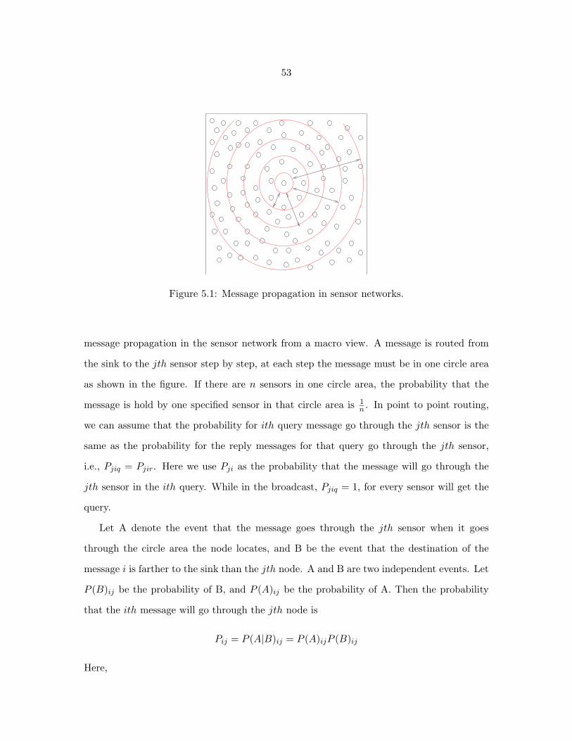
53

Figure 5.1: Message propagation in sensor networks.

message propagation in the sensor network from a macro view. A message is routed from

the sink to the jth sensor step by step, at each step the message must be in one circle area

as shown in the figure. If there are n sensors in one circle area, the probability that the

message is hold by one specified sensor in that circle area is 1n . In point to point routing,

we can assume that the probability for ith query message go through the jth sensor is the

same as the probability for the reply messages for that query go through the jth sensor,

i.e., Pjiq = Pjir. Here we use Pji as the probability that the message will go through the

jth sensor in the ith query. While in the broadcast, Pjiq = 1, for every sensor will get the

query.

Let A denote the event that the message goes through the jth sensor when it goes

through the circle area the node locates, and B be the event that the destination of the

message i is farther to the sink than the jth node. A and B are two independent events. Let

P (B)ij be the probability of B, and P (A)ij be the probability of A. Then the probability

that the ith message will go through the jth node is

Pij = P (A|B)ij = P (A)ijP (B)ij

Here,

54

P (B)ij = Nfar

Ntotal= Nn−πdjis

2ρNn

and

P (A)ij =1

π(((bdjis

r c+ 1) ∗ r)2 − (bdjis

r c ∗ r)2)ρ

=1

π(2bdjis

r c+ 1)r2ρ

Thus

Pij = 1

π(2bdjis

rc+1)r2ρ

Nn−πdjis2ρ

Nn

Now we can calculate the remaining lifetime of sensor in the case of unicast in Traditional

and broadcast in both Traditional and IQ. In above formula, the difference between

Traditional and IQ lies in djis, which is constant in Traditional for each sensor be-

cause the sink is fixed all the time and is changing in IQ because of the shifting of the

delegate.

5.4 Remaining Lifetime of Sensors in Unicast using Traditional

In the case of unicast, the message will go through only the sensors on the path between

the sink and the destination once for each query, so does the reply message for that query.

Thus the remaining lifetime of each sensor in unicast using Traditional can be defined as

L(j) = 1−Nm∑i=1

εjiqNjiq + εjirNjir

Ej

= 1−Nm∑i=1

εjiq ∗ Pji ∗ 1 + εjir ∗ Pji ∗ 1Ej

Because we assume the sensors are homogeneous and the same type messages are having

the same size, Ej is equal to E, εjiq = εq and εjir = εr, the remaining lifetime of each sensor

in the point to point routing is

L(j) = 1− 1E

(εq+εr)Nm

π(2bdjis

rc+1)r2ρ

Nn−πd2jisρ

Nn

55

5.5 Remaining Lifetime of Sensors in Broadcast using Traditional

Next, we analyze the remaining lifetime of each sensor when the query message is broad-

casted to all the sensors from the sink. In this case, the query message floods to all the

sensors while the reply messages will go through the sensors on its path to the sink. For each

query message if we assume the probability that one sensor will generate a reply message

is 1f , the remaining lifetime of each sensor in broadcast using Traditional is

L(j) = 1−Nm∑i=1

εjiq ∗Njiq + εjir ∗Njir

Ej

= 1−Nm∑i=1

εjiq ∗Nnbrs + εjirPjirNn1f

Ej

Because the query is routed by flood, i.e., each sensor will get a query from its neighbors

and send a query to its neighbors. So the remaining lifetime of sensor in the broadcast

traditional query is

L(j) = 1− NmεqNnbrs

E − εrNmEfπr2ρ

Nn−πdjis2ρ

2bdjis

rc+1

5.6 Remaining Lifetime of Sensors in IQ

In the indirect query, a query is directed to a randomly selected delegate, then the delegate

acts as the sink to take care of query forwarding, data collection, and data transmitting back

to the sink. If the probability of each sensor to be a delegate is the same, when there are

totally Nm queries been processed, and there are totally Nn sensors in the sensor network,

for each sensor the possible times it is selected as a delegate is NmNn

. The number of times

that the sensor is located in the area with djis = kr to the delegate is the number of the

sensors located in the circle area between kr and kr + 1 to that sensor. The number of the

sensors located in the circle area between kr and kr+1 is π(2k+1)r2ρ. Thus the remaining

56

lifetime of each sensor in IQ can be defined as

L(j) = 1−Nm∑i=1

εjiq ∗Njiq + εjir ∗Njir

Ej

= 1− εqNmNnbrs

E− 1

E

Nn

f

Nm∑i=1

εrNjir −Nm

Nn

Nn

fEεr,rcv

= 1− εqNmNnbrs

E− 1

E

Nn

f

dmax∑k=1

(εrNm

Nn∗ Pjis(πρ(((k + 1)r)2 − (kr)2)))

−Nm

fEεr,rcv

= 1− εqNmNnbrs

E− εrNmdmax

Ef+

εrNm

Ef

πρr2

2Nndmax(dmax + 1)− Nm

fEεr,rcv

(b) the sonsors far from the sink are dead(a) The sensors near the sink are dead

Figure 5.2: An example of the importance of different sensors, assuming the data sink islocated at the low-left corner.

Based on the remaining lifetime of sensors, we define the remaining lifetime of the whole

sensor network in the following section. First we define the importance of sensors.

5.7 Importance of Different Sensor Nodes

The failure† of sensors will cause the sensor network to act improperly, but the level of

the damage it causes is different, which is the reason why we think the previous definition

†In this dissertation, we consider only the failure resulted from the depletion of energy.

57

of the lifetime as the time before the first sensor failure or first message failure without

considering the location of the sensor is unsatisfactory. For the same number of failure

sensors, the damage may be very slight at sometime and the sensor network still performs

almost normally, while sometimes it may be very serious which makes the sensor network

lose its most functionality. Two cases are described in the Figure 5.2(a) and (b) as an

example. In the figure, the black nodes represent the sensors that have run out of energy

and the white ones denote the ones that are still alive. In both Figure 5.2(a) and (b)

the sensor networks cannot act as it suppose to do since in both cases the sensor network

cannot gain data from some sensors, but in Figure 5.2(a), although there are only three

failed sensors, the sink cannot get data from most of the sensors. In Figure 5.2(b), there

are seven dead nodes, but the sink can still get data from most of the sensors in the sensor

network. So the damage to the sensor network by the failure sensors is not only related to

the number of failed sensors but also related to the location of the failed sensors. To this

end, sensors in the sensor network have different importance. We define a factor named

weight for each sensor to count the importance of that sensor. Based on above analysis,

the nearer the sensor to the sink, the more important it is. So we define the weight of each

sensor as following:

wj = c 1djis

2

Here c is a constant.

5.8 Remaining Lifetime of the Whole Sensor Network

In Section 5.2, 5.4, 5.5, 5.6, we have defined the remaining lifetime for sensors. Now we are

in a position to examine the remaining lifetime of the whole sensor network. We consider

the remaining lifetime of the whole sensor network as the sum of the weighted remaining

lifetime of all sensors in the sensor network. Thus the remaining lifetime of the whole sensor

network is

L =∑Nn

j=1 wjL(j)

58

From this definition, we can easily get the remaining lifetime of the whole sensor network

in unicast, broadcast using Traditional and in IQ. Specifically, in unicast, the remaining

lifetime of the whole sensor networks is defined as:

L =∑Nn

j=1 c 1djis

2 (1− 1E

(εq+εr)Nm

π(2bdjis

rc+1)r2ρ

Nn−πd2jisρ

Nn)

≈ cπρ(2 ln(dmax) + π2

6 )− c(εq+εr)Nmπ2

6Er2 + c(εq+εr)Nm

Er2dmax

In the case of broadcast using Traditional, the remaining lifetime of the whole sensor

network is defined as:

L =Nn∑j=1

c1

djis2 (1− NmεqNnbrs

E− εrNm

Efπr2ρ

Nn − πdjis2ρ

2bdjis

r c+ 1)

≈ cπρ(2 ln dmax +π2

6)(1− εqNmNnbrs

E)− cπ2εrNmNn

6Efr2+

cεrNmπρdmax

Ef

Similarly in IQ, the remaining lifetime of the whole sensor network is defined as:

L =Nn∑j=1

c1

djis2 (1− εqNmNnbrs

E− εrNmdmax

Ef

+εrNn

Ef

πρr2

2Nndmax(dmax + 1)− Nm

Efεr,rcv)

≈ cπρ(1− εqNmNnbrs

E− εrNmdmax

Ef

+εrNm

Ef

πρr2

2Nn∗ dmax(dmax + 1)− Nm

fEεr,rcv)(2 ln dmax +

π2

6)

Based on the remaining lifetime of the whole sensor network, the lifetime of the sensor

network can be formally defined as:

LFT = { Nm | L(Nm − 1) < L(Nm) & L(Nm + 1) = L(Nm) or Nfail ≥ θ }

where θ is a pre-defined threshold of maximum number of the failure sensors in the sensor

network and Nfail is the number of the failure sensors.

Based on these models, we depict the detailed analysis of different query protocols in

the following section.

59

Query Types Unicast(Traditional)

Broadcast(Traditional)

IQ

0 < d < r 1− 158Nm106 1− 8280Nm

106 1− 2149Nm106

d = 7r 1− 8Nm106 1− 2000Nm

106 1− 2149Nm106

d = 14r 1 1− 1670Nm106 1− 2149Nm

106

Table 5.2: Comparison of the remaining lifetime of different nodes in different locations.

5.9 Analytical Comparison: Traditional vs. IQ

One of the goals of modeling is to evaluate the performance of different protocols. Now we

are in the position to compare Traditional with IQ in terms of the remaining lifetime of

sensors and the remaining lifetime of the whole sensor network.

To quantitatively compare these two query protocols, we adopt the practical values of

sensor parameters obtained from Berkeley motes [Hill et al., 2000], including the initial

energy and the energy consumption rate. In [Hill et al., 2000] two 1.5V batteries rated

at 575mAh are used for each sensor, so the initial total energy of each sensor is 1.725J .

The energy to transmit and receive a single bit is 1µJ and 0.5µJ respectively. We assume

the size of query message and reply message to be 240bits and 1200bits separately. Thus

it takes 240µJ to transmit a query message and 120µJ to receive a query message; and

it takes 1200µJ and 600µJ to transmit and receive a reply message. If we assume the

total number of sensors in the sensor network is 1500 and the density of the sensor network

is 1 per 1000m2, the maximum distance between every two sensors is 14r, where r is the

communication range equal to 50m. We also assume the probability of one sensor generating

a corresponding reply message is 1/30, thus f = 30.

First we compare the sensors located at different areas in the sensor network based on

the remaining lifetime of the sensors. Table 5.2 depicts the remaining lifetime of the sensors

located at different regions in the sensor field in the context of different query protocols. Here

we select the sensors with its distance to the sink as within one communication range, with

seven times communication range, and with 14 times communication range respectively.

60

Query Types Unicast(Traditional)

Broadcast(Traditional)

IQ

Remaining lifetime 21733−0.8Nm106

21733−69Nm106

21733−46Nm106

Table 5.3: Comparison of the remaining lifetime of the whole sensor network.

The last range is the largest distance to the sink. From the figures in the table, we can find

that the remaining lifetime of the sensor increases along with the increase of the distance

between the sensor to the sink in Traditional, but it increases quicker in the broadcast

communication than in unicast communication, because the load imbalance is accumulated

faster in broadcast case. Thus the sensors near to the sink will consume a lot of energy

and fail very quickly, which results in the earlier termination of the whole sensor network.

From this observation, we find that the unbalanced load results in the short lifetime of the

sensor network. On the contrary, as we expected, the remaining lifetime of sensors located

in different regions using the IQ protocol are almost same, which denotes that IQ indeed

does a good job on balancing the load among all sensors.

We also compare the remaining lifetime of the sensor network here. The results of

comparison of three types of query protocol are listed in Table 5.3. From these deduced

results, we can find that the sensor network using the IQ protocol has longer remaining

lifetime than that of using Traditional by providing a global optimization to balance the

load to the whole sensor network. Furthermore, considering these two tables together, in

broadcast using Traditional, when Nm = 121, although there are still a large amount of

energy (13384106 from Table 5.3) remaining in the sensor network, it will never be used because

the sensor network is down when all sensors within the sink’s communication range are

down (see in Table 5.2 when Nm = 121). While in IQ, because the load is balanced, no

sensors will run out of energy much earlier than others. So most energy of each sensor

61

Variables ValuesCommunication Range 30mNumber of Nodes 400Total Energy of Each Sensor 3 JoulesPacket Size 240, 1200 bitsEnergy Dissipated for Receiving 50 nJ/bitEnergy Dissipated for Transmission 50 nJ/bitEnergy Dissipated for Transmit Am-plifier

100 pJ/bit/m2

Bandwidth 40kbps

Table 5.4: Simulation parameters.

will be effectively used in IQ. To this end, we think that IQ is more energy efficient than

Traditional, i.e, the energy utilization is much lower in IQ than that in Traditional.

From the above analysis, we conclude that IQ extends the lifetime of the whole sensor

network because it balances the load to all the sensors in the sensor network, which again

validates our argument that the load balance plays a very important role in the lifetime of

the whole sensor network.

5.10 Simulation Verification

To verify the analytical results, we conduct a detailed simulation using the Capricorn [Sha

et al., 2004], a large-scale discrete-event driven simulator. In our simulation, 400 nodes are

scattered to a 600m×600m square field. We use the GPSR routing protocol implemented

in routing layer of the simulator to deliver message. All simulation parameters are listed in

Table 5.4. In this section, we evaluate Traditional and IQ in terms of energy consumption,

RLSN and LSN.

5.10.1 Energy Consumption

First we compare energy consumption of each sensor in Traditional and IQ, which can

reflect RLIS. Figure 5.3 reports the energy consumption of sensors in two protocols after

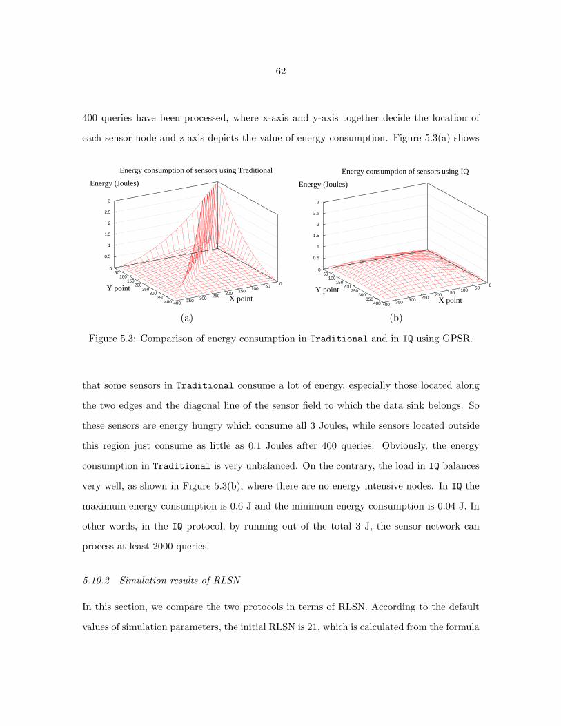
62

400 queries have been processed, where x-axis and y-axis together decide the location of

each sensor node and z-axis depicts the value of energy consumption. Figure 5.3(a) shows

Energy consumption of sensors using Traditional

0 50 100 150 200 250 300 350 400X point

0 50

100 150

200 250

300 350

400

Y point

0.5

1

1.5

2

2.5

3

Energy (Joules)

Energy consumption of sensors using IQ

0 50 100 150 200 250 300 350 400X point

0 50

100 150

200 250

300 350

400

Y point

0.5

1

1.5

2

2.5

3

Energy (Joules)

(a) (b)

Figure 5.3: Comparison of energy consumption in Traditional and in IQ using GPSR.

that some sensors in Traditional consume a lot of energy, especially those located along

the two edges and the diagonal line of the sensor field to which the data sink belongs. So

these sensors are energy hungry which consume all 3 Joules, while sensors located outside

this region just consume as little as 0.1 Joules after 400 queries. Obviously, the energy

consumption in Traditional is very unbalanced. On the contrary, the load in IQ balances

very well, as shown in Figure 5.3(b), where there are no energy intensive nodes. In IQ the

maximum energy consumption is 0.6 J and the minimum energy consumption is 0.04 J. In

other words, in the IQ protocol, by running out of the total 3 J, the sensor network can

process at least 2000 queries.

5.10.2 Simulation results of RLSN

In this section, we compare the two protocols in terms of RLSN. According to the default

values of simulation parameters, the initial RLSN is 21, which is calculated from the formula

63

in Section 7.2. Figure 5.4 shows the simulation results, where x-axis is the number of queries,

and y-axis represents RLSN.

25

20

15

10

5

0 400 350 300 250 200 150 100 50 10R

emai

ning

life

time

of th

e se

nsor

net

wor

k

Number of queries

IQ

Traditional

IQ

Figure 5.4: Comparison of RLSN by using Traditional and IQ.

From the figure, we find that RLSN decreases along with the increase of the number

of processed queries. In Traditional, RLSN drops very quickly from 21 to less than 10

during 300 queries have been processed. After 300 queries have been processed, RLSN

using Traditional keeps stable. This is because the sensor network is already dead after

300 queries. In other words, no more query message can be sent from the sink to other alive

sensors, thus no more energy is consumed. This does not mean that the remaining energy in

the alive sensors is saved. On the contrary, these energy is just wasted, which can never be

used in the future. In case of IQ, RLSN drops very slowly and smoothly. After 400 queries

have been processed, RLSN is still good using IQ. A lot of energy is saved to be used for

the future queries. From this point of view, we argue that IQ is more energy efficient than

Traditional.

64

250

200

150

100

50

0 0.3 0.25 0.2 0.15 0.1 0.05

Lif

etim

e of

the

sens

or n

etw

ork

Total initial energy of each sensor

IQ

Traditional

Figure 5.5: Comparison of LSN by using Traditional and IQ.

5.10.3 Simulation results of LSN

Finally, we compare LSN, which is more interesting to application scientists and system

designers. We set the value of θ (the threshold to determine the aliveness of the sensor

network) to 90%. The comparison between Traditional and IQ protocols is reported in

Figure 5.5, where x-axis is the initial energy of each sensor and y-axis is the value of LSN.

From the figure, it can be easily seen that LSN increases almost linearly with the increase

of initial energy in both Traditional and IQ. However, LSN increases much faster in IQ

than that in Traditional, where the lifetime in the Traditional model is about 16 of that

in IQ. Additionally, if we increase the value of θ, the gap between the Traditional and IQ

will become much larger. Thus we conclude that IQ indeed extends LSN several times as

that of Traditional.

In this chapter, we formally define the remaining lifetime of individual sensor, the re-

maining lifetime of sensor networks, and the lifetime of wireless sensor network, which is

an application specific performance metric to evaluate the performance of the proposed

protocol. Based on these models, we compare two query protocols; both theoretical and

simulation results show that IQ balances the load so that extends the lifetime of the sensor

65

network. Having this system level performance metric to evaluate energy efficiency, we are

ready to provide an energy efficient system design, which is denoted in the next several

chapters.

66

CHAPTER 6

QUALITY-ORIENTED SENSING DADA ANALYSIS

With the increasing number of deployments of sensor systems, in which the main function

is to collect interesting data at the sink, it is becoming crucial to carefully analyze the large

amount of collected data. However, this problem is neglected in previous research, which

mainly focuses on energy efficient, reliable sensor systems design and optimization. Al-

though data quality management attracts more and more attention in the last two years [Li

et al., 2006, Sha and Shi, 2008], proposing novel data quality management mechanisms is

still an important and interesting research topic. We argue that sensor system optimiza-

tion and data quality management are closely related to the characteristics of collected

data, in other words, sensor system optimization and data quality management should take

data characteristics into consideration. Thus, in this dissertation, we take an initial step

to characterize the data quality using a set of one-month data collected by a real-world

water system surveillance application. The data set consists of water level, precipitation,

and gauge voltage measurements from 13 gauges located around Lake Winnebago, St. Clair

River and Detroit River in January 2008.

Our data analysis focuses on quality oriented data analysis. In quality oriented data

analysis, we intend to discover two types of data, namely similarity data and abnormal

data. The significance of our discovery is two-fold. On one hand, it helps us understand

the laws and changes in the monitored field. On the other hand, it unveils the limitations

in the current sensor system design, and provides us with a strong ground upon which we

can base our future WSN systems design.

67

Our study reveals several interesting facts. First, information similarity, including pat-

tern similarity and numerical similarity, is very common, which provides a good opportu-

nity to trade off energy efficiency and data quality. Second, different parameters exhibit

different data characteristics, which suggests that adaptive protocols using variable sam-

pling rates can bring in significant improvements. Third, spatial correlation analysis and

multi-modality correlation analysis provide a way to evaluate data integrity and to de-

tect conflicting data that usually indicates appearances of sensor malfunction or interesting

events. Fourth, abnormal data may appear all the time, and continuous appearance of

abnormal data usually suggests a failure or an interesting event. Finally, external harsh

environmental conditions may be the most important factor on inflicting failures in envi-

ronmental applications. Despite these failures and possible sensing failures, data quality is

still satisfactory.

6.1 Background

The United States Army Corps of Engineers (USACE) in Detroit District, has 22 data

collection platforms commonly referred to as sensor nodes or gauges, deployed around the

St. Clair and Detroit rivers in southeast Michigan as well as the Lake Winnebago watershed

southwest of Green Bay, Wisconsin. One month data in January 2008 from 13 of the 22

gauges were made available for this study. Each sensor node collects battery voltage, water

level and precipitation except the Dunn Paper gauge (G1) which collects battery voltage, air

temperature and water temperature. However, precipitation data for the St. Clair/Detroit

river system is not used in this work, because that “data” in the raw files is simply an

artifact of the gauge programming. For convenience, we name each sensor node as G1,

where ‘G’ stands for “gauge.” The gauge locations of G1, G2 and G3 are on the St. Clair

River, G4 is located on the Detroit River, and G5 through G13 are spread around the Lake

Winnebago watershed. Gauges G5 through G13 are shown in Figure 6.1, and the other

remaining gauges are shown in Figure 6.2. It is worth mentioning that G8 and G10 suffered

68

many failures throughout the period of study. Therefore, any data analysis on G8 or G10

will mostly look like “weird” or at least different from the other gauges.

G5G9

G8

G7G13

G11

G10G6

G12

Figure 6.1: Lake Winnebago Watershed.

Data samples are sent from each gauge to the GOES satellite, once every hour or every

four hours, depending on whether the station has a high baud rate transmitter or not.

High baud rate transmitters send data every hour. Data is then sent from the satellite to

a central location in Wallops Island in Virginia, where the data samples are collected and

arranged in files for later download through a regular ftp service. We conducted our analysis

directly using the un-decoded files. This raw data set has not been subject to any quality

control procedure, and thus provide a good opportunity to study false readings happening

in sensing systems. Water level and precipitation are sampled once every hour, whereas

voltage is sampled once every hour or every two hours. Water level is measured against the

IGLD Datum 1985, which works as the base to measure current water level. So negative

water level means it is below the local IGLD Datum 1985, though that does not happen

often. Precipitation data is supposed to be constantly increasing (except when the gauge

resets as part of its normal operation). To figure out how much precipitation fell over a

one-hour period, the difference between consecutive samples are calculated and reported.

The measurements for voltage and precipitation are in volts and inches respectively. Water

69

G1

G2

G3

G4

Figure 6.2: St. Clair River and Detroit River.

level is reported in meters, centimeters and feet. For convenience, we converted the readings

for water level in meters.

Based on the raw data, we focus on individual time series analysis for each sensor

and one of its measure attribute, correlation between different data series. For each data

series, we investigated information redundancy pattern and proposed methods to detect

abnormal data. The redundancy pattern is analyzed in terms of pattern similarity and

numerical similarity. Correlation between data series is examined against different attributes

for the same sensor node and the same attribute for different sensor nodes. The relation

between water level and precipitation is carefully studied with different endurance interval

settings. As to spatial correlation, we looked into the similarity of water level collected

by different sensor nodes, and the similarity of precipitation collected by different sensor

nodes. In addition, to detect abnormal water level, we analyzed empirical distribution for

70

the difference of scaled water level. The water level is scaled according to our statistical

analysis.

6.2 Quality-Oriented Sensing Data Analysis

The goal of data analysis is to understand and discover the rules and patterns in the data

set, as well as to detect interesting events in the monitored field. Also, we argue that the

implication of the data analysis can unveil the limitations in the current wireless sensor

network designs. In this section, we focus on quality-oriented sensing data analysis. How to

define data quality is still an open problem. Here, We define high quality data as the data

that contains the most information from the monitored field.

We analyze the data collected from an environmental monitoring application, which

uses 13 gauges to monitor water level, accumulative participation and voltage of in Lake

Winnebago, St. Clair River, Detroit River during the entire month of January 2008. To

understand the quality of the collected data, we try to discover the spatial and temporal

relationship among those data; specifically, we are mostly interested in detecting two types

of data, redundant data and abnormal data. Usually, redundant data, which we name

as similarity, will not affect the overall quality of the collected data when it is removed.

Contrary to redundant data, abnormal data, which largely affects the data quality, should

be examined more carefully, because it usually denotes sensor failures, malicious attacks

or interesting events. In the rest of this section, we first examine each sensor parameter

individually from the temporal perspective to discover any pattern and numerical similarity,

as well as abnormal data. Then, we check the relationship between two parameters, water

level and accumulated precipitation. Finally, we figure out the relationship between same

type sensors located in different locations.

6.2.1 Time Series Analysis for Individual Parameter

For each individual parameter, we define two types of similarity, the pattern similarity and

the numerical similarity. Here, we define a pattern as the continuous reappearance of the

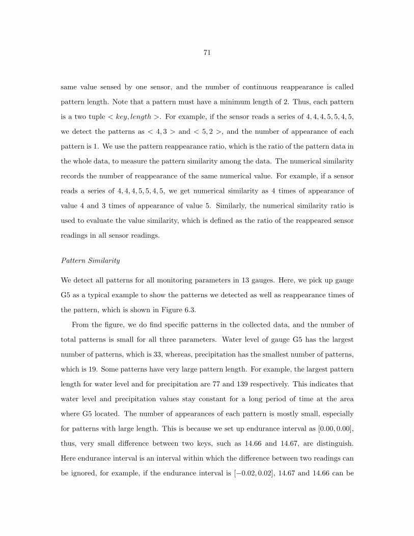
71

same value sensed by one sensor, and the number of continuous reappearance is called

pattern length. Note that a pattern must have a minimum length of 2. Thus, each pattern

is a two tuple < key, length >. For example, if the sensor reads a series of 4, 4, 4, 5, 5, 4, 5,

we detect the patterns as < 4, 3 > and < 5, 2 >, and the number of appearance of each

pattern is 1. We use the pattern reappearance ratio, which is the ratio of the pattern data in

the whole data, to measure the pattern similarity among the data. The numerical similarity

records the number of reappearance of the same numerical value. For example, if a sensor

reads a series of 4, 4, 4, 5, 5, 4, 5, we get numerical similarity as 4 times of appearance of

value 4 and 3 times of appearance of value 5. Similarly, the numerical similarity ratio is

used to evaluate the value similarity, which is defined as the ratio of the reappeared sensor

readings in all sensor readings.

Pattern Similarity

We detect all patterns for all monitoring parameters in 13 gauges. Here, we pick up gauge

G5 as a typical example to show the patterns we detected as well as reappearance times of

the pattern, which is shown in Figure 6.3.

From the figure, we do find specific patterns in the collected data, and the number of

total patterns is small for all three parameters. Water level of gauge G5 has the largest

number of patterns, which is 33, whereas, precipitation has the smallest number of patterns,

which is 19. Some patterns have very large pattern length. For example, the largest pattern

length for water level and for precipitation are 77 and 139 respectively. This indicates that

water level and precipitation values stay constant for a long period of time at the area

where G5 located. The number of appearances of each pattern is mostly small, especially

for patterns with large length. This is because we set up endurance interval as [0.00, 0.00],

thus, very small difference between two keys, such as 14.66 and 14.67, are distinguish.

Here endurance interval is an interval within which the difference between two readings can

be ignored, for example, if the endurance interval is [−0.02, 0.02], 14.67 and 14.66 can be

72

regarded as the same. Because of unavoidable system error in measurement and applications

lowered requirements on accuracy, it is reasonable to set up an endurance interval for each

monitoring parameter. Another reason is that we define different patterns even when they

have the same key value but different lengths.

Figure 6.4 shows the pattern reappearance ratio, where “-” means there is no avail-

able data. In the figure, we find that voltage has the smallest pattern reappearance ratio,

which suggests that the changes of the voltage are very frequent. This is also because we

distinguished the pattern keys in extremely fine granularity; however, even in such a fine

granularity, both patterns in water level and precipitation show a large ratio of pattern sim-

ilarity. For example, the smallest pattern reappearance ratio is 0.43 in G3, and the largest

pattern reappearance ratio is 0.94 in G12. While precipitation shows the largest pattern

similarity, which can be seen not only from the least number of patterns in Figure 6.3, but

also from the fact that it has all pattern reappearance ratio larger than 0.77; actually, most

pattern reappearance ratio of precipitation is about 0.99 for all gauges. We can expect pre-

cipitation to stay stable at most time. It may change suddenly, however, after this sudden

change, it goes back to normal and stabilizes for a long period of time. Voltage has the

most varying pattern reappearance ratios, which ranges from 0.04 to 0.96, showing that the

performance of the power supply is really independent and highly dynamic. The goal of the

sensor network applications is to collect meaningful data, thus, most of those applications

can endure a certain level of data inaccuracy, which will not affect our discovery of the rules

and events in the monitoring field. We reexamine the pattern reappearance ratio after we

lower the accuracy requirements on the collected data and set up different endurance inter-

vals for three parameters. The resulted pattern reappearance ratio is depicted in Figure 6.5,

where the three numbers under the title are the endurance intervals, which are mostly 10%

of possible largest changes, i.e., we allow voltage to endure 0.2 volts changes, water level

to endure 0.04 meter changes, and precipitation to endure 0.04 inch changes. Note that

73

different units are used for water level and precipitation, i.e., meter for water level and inch

for precipitation, which we keep the original units as in the raw data.

Comparing Figure 6.5 to Figure 6.4, we can find that almost all pattern reappearance

ratios increased by increasing the endurance interval, especially for those with small reap-

pearance ratio in Figure 6.4. After we increase the endurance interval, we can see that

50% of the voltage data pattern reappearance ratio is larger than 0.95, while water level

and precipitation pattern reappearance ratio do not change too much compared to that in

voltage; however, most of them are still larger than those in Figure 6.4. From both figures,

we can see that there is a big pattern reappearance ratio.

In our definition, pattern length means the number of continuous appearance of the same

sensor reading. Thus, we try to figure out the distribution of the pattern length in terms of

variable endurance interval, as shown in Figure 6.6, Figure 6.7, and Figure 6.8, where the

x-axis is the length of the pattern and the y-axis is the CDF of the pattern length. From

the figure, we find that most patterns have short patten length. For example, when the

endurance interval is set to be [0.00, 0.00], 90% of voltage patterns have length less than

10, and about 70% of water level patterns and about 60% of precipitation patterns have

length less than 10. However, different parameters have different pattern lengths. In the

figure, we can see that voltage, which has almost all pattern length less than 20, has more

short length patterns than water level and precipitation, while precipitation has the longest

length among the three parameters, where about 30% of the precipitation pattern has length

longer than 20. This observation shows that precipitation is stable at most of the time, but

the reading of the voltage has high dynamics. By increasing the endurance interval, more

patterns have longer length appear. For example, when water level endurance interval is

increased to [−0.04, 0.04], more than 30% of the patterns have length between 140 to 180.

74

Numerical Similarity

Having studied pattern similarity, we move on to check the numerical similarity. Numerical

similarity focuses on the numerical value reappearance of the sensing data, which differs

from pattern similarity in that numerical similarity does not intend to detect any pattern.

For the numerical similarity, we identify the number of appearance for each individual value.

Figure 6.9, Figure 6.10 and Figure 6.11 shows the numerical distribution of the collected

data, where the x-axis is the numerical value of the sensing reading and the y-axis denotes

the number of appearance of the corresponding numerical value. Note that we pick up the

data collected by gauge G5 as an example.

75

V Pattern  Appearances W Pattern Appearances P Pattern Appearances<14.09, 2> 1 <0.67, 2> 1 <1.67, 2> 1<14.58, 2> 1 <0.68, 2> 1 <1.77, 2> 1<14.59, 2> 1 <0.69, 2> 2 <2.28, 2> 1<14.63, 2> 2 <0.70, 2> 1 <2.50, 2> 1<14.64, 2> 1 <0.71, 2> 2 <2.52, 2> 1<14.66, 2> 2 <0.72, 2> 1 <2.30, 5> 1<14.67, 2> 2 <0.68, 3> 1 <2.47, 5> 1<14.68, 2> 3 <0.69, 3> 2 <2.24, 7> 1<14.69, 2> 1 <0.70, 3> 2 <2.34, 7> 1<14.71, 2> 1 <0.71, 3> 4 <2.40, 8> 1<14.73, 2> 1 <0.72, 3> 2 <1.69, 16> 1<14.57, 3> 1 <0.70, 4> 2 <2.36, 22> 1<14.60, 3> 1 <0.71, 4> 1 <2.20, 38> 1<14.67, 3> 3 <0.72, 4> 3 <2.36, 44> 1<14.72, 3> 1 <0.69, 5> 2 <2.11, 49> 1<14.65, 4> 1 <0.70, 5> 4 <2.53, 67> 1<14.67, 4> 2 <0.70, 9> 1 <2.41, 97> 1<14.68, 4> 3 <0.72, 9> 1 <2.51, 102> 1<14.69, 4> 2 <0.71, 11> 1 <1.29, 139> 1<14.61, 5> 1 <0.71, 14> 1<14.64, 5> 1 <0.68, 16> 1<14.67, 5> 1 <0.71, 16> 1<14.68, 5> 2 <0.71, 18> 1<14.68, 6> 1 <0.71, 22> 1<14.70, 6> 1 <0.67, 28> 1<14.67, 7> 2 <0.68, 29> 1<14.69, 7> 1 <0.71, 30> 1<14.68, 8> 2 <0.70, 34> 1<14.68, 9> 2 <0.70, 38> 1<14.68, 10> 1 <0.69, 45> 1<14.68, 11> 1 <0.69, 47> 1<14.67, 12> 1 <0.68, 69> 1

<0.72, 77> 1

Figure 6.3: Detected patterns and the number of appearance in gauge G5.

76

Gauge ID

Voltage Pattern

Reappearance Ratio

Water Level Pattern

Reappearance Ratio

Precipitation Pattern

Reappearance Ratio

G1 0.07 - - G2 0.85 0.64 - G3 0.78 0.43 - G4 0.38 0.57 - G5 0.50 0.88 0.92 G6 0.17 0.84 0.89 G7 0.96 0.69 0.93 G8 - - - G9 0.23 0.87 0.89 G10 0.04 0.44 0.77 G11 0.10 0.83 0.90 G12 0.87 0.94 0.91 G13 0.05 0.88 0.89

 

Figure 6.4: Pattern reappearance ratio with zero endurance interval.

Gauge ID

Voltage Pattern

Reappearance Ratio

[-0.1, 0.1]

Water Level Pattern

Reappearance Ratio

[-0.02, 0.02]

Precipitation Pattern

Reappearance Ratio

[-0.02, 0.02] G1 0.59 - - G2 1.00 0.85 - G3 1.00 0.74 - G4 0.96 0.78 - G5 0.88 0.99 0.95 G6 0.98 0.94 0.92 G7 1.00 0.99 0.95 G8 - - - G9 1.00 0.94 0.92 G10 0.64 0.72 0.79 G11 0.78 0.93 0.94 G12 1.00 0.99 0.94 G13 0.80 0.95 0.94

 

Figure 6.5: Pattern reappearance ratio with increased endure interval.

77

0 20 40 60 80 100 120 1400

0.1

0.2

0.3

0.4

0.5

0.6

0.7

0.8

0.9

1

Voltage Pattern Length

Em

piric

al C

ulm

ulat

ive

Pro

babi

lity

[0.00,0.00][-0.02,0.02][-0.04,0.04][-0.06,0.06][-0.08,0.08][-0.10,0.10]

Figure 6.6: CDF of pattern length of Voltage.

0 50 100 150 200 250 300 3500

0.1

0.2

0.3

0.4

0.5

0.6

0.7

0.8

0.9

1

Water Level Pattern Length

Em

piric

al C

ulm

ulat

ive

Pro

babi

lity

[0.00,0.00][-0.02,0.02][-0.04,0.04][-0.06,0.06][-0.08,0.08][-0.10,0.10]

Figure 6.7: CDF of pattern length: of water level.

78

0 20 40 60 80 100 120 140 160 180 2000

0.1

0.2

0.3

0.4

0.5

0.6

0.7

0.8

0.9

1

Precipitation Pattern Length

Em

piric

al C

ulm

ulat

ive

Pro

babi

lity

[0.00,0.00][-0.02,0.02][-0.04,0.04][-0.06,0.06][-0.08,0.08][-0.10,0.10]

Figure 6.8: CDF of pattern length of precipitation.

 

 

0

10

20

30

40

50

60

70

80

90

100

13.4 13.6 13.8 14 14.2 14.4 14.6 14.8 15

Figure 6.9: The number of appearances for each numerical values of voltage.

79

 

 

0

20

40

60

80

100

120

140

160

0.66 0.67 0.68 0.69 0.7 0.71 0.72 0.73 0.74

Figure 6.10: The number of appearances for each numerical values of water level.

 

 

0

20

40

60

80

100

120

140

160

0 0.5 1 1.5 2 2.5 3

Figure 6.11: The number of appearances for each numerical values of precipitation.

In the figure, we find that those three parameters exhibit totally different distributions.

The reading of the voltage and water level are very close to normal distribution with µ =

14.22, σ = 0.38 and µ = 0.7, sigma = 0.02 respectively. The voltage readings are more

centralized to value 14.7, while water level readings are more broadly distributed from 0.68

to 0.72 and centralized at 0.71. The reading of precipitation shows no obvious distribution.

It spreads from about 1.25 to 2.55. Some precipitation values such as 1.29 and 2.51, appear

80

much more times than others, which means no rain or snow falls for a long time after the

precipitation value is read, while other precipitation readings only appear several times,

which mainly depicts some transitional states during a continuous rain or snow falling. Like

the pattern similarity ratio, numerical reappearance ratio is used to evaluate the numerical

similarity.

Gauge ID

Voltage Numerical

Reappearance Ratio

Water Level Numerical

Reappearance Ratio

Precipitation Numerical

Reappearance Ratio

G1 0.84 - - G2 0.99 0.64 - G3 0.97 0.43 - G4 0.91 0.57 - G5 0.82 0.88 0.92 G6 0.94 0.84 0.89 G7 0.99 0.69 0.93 G8 - - - G9 0.97 0.87 0.89 G10 0.77 0.44 0.77 G11 0.82 0.83 0.90 G12 0.99 0.94 0.91 G13 0.89 0.88 0.89

 

Figure 6.12: Numerical reappearance ratio with endurance interval [0.00, 0.00].

Figure 6.12 presents the numerical reappearance ratio of the sensing data at all gauges.

We can see that all parameters exhibit very high reappearance ratio. Compared to pattern

reappearance ratio, numerical reappearance ratio is much larger for voltage, fairly larger

for water level, and comparable for precipitation. For example, the voltage pattern reap-

pearance ratio in G1, G10 and G11 is less than 10%, while the voltage numerical pattern

reappearance is close to 80%. The large difference implies that although the numerical

readings of the voltage have a large similarity, they fluctuate very frequently and there are

no obvious patterns in voltage readings. The two reappearance ratios of precipitation do

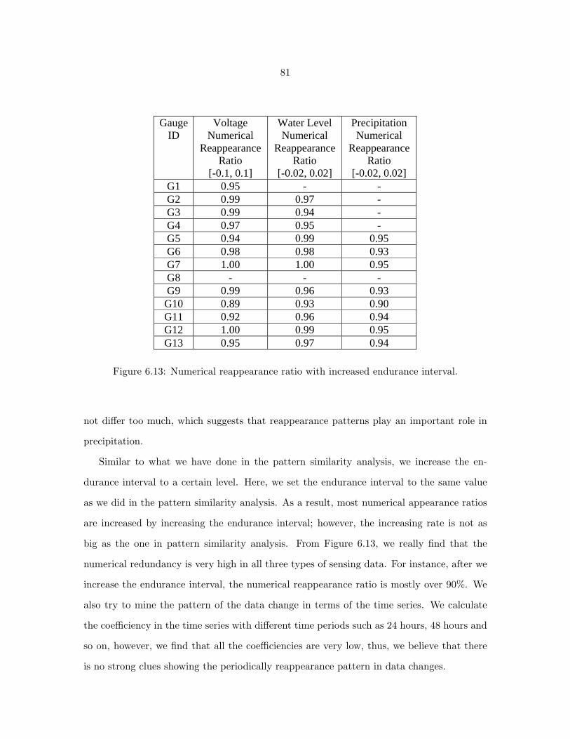
81

Gauge ID

Voltage Numerical

Reappearance Ratio

[-0.1, 0.1]

Water Level Numerical

Reappearance Ratio

[-0.02, 0.02]

Precipitation Numerical

Reappearance Ratio

[-0.02, 0.02] G1 0.95 - - G2 0.99 0.97 - G3 0.99 0.94 - G4 0.97 0.95 - G5 0.94 0.99 0.95 G6 0.98 0.98 0.93 G7 1.00 1.00 0.95 G8 - - - G9 0.99 0.96 0.93 G10 0.89 0.93 0.90 G11 0.92 0.96 0.94 G12 1.00 0.99 0.95 G13 0.95 0.97 0.94

 Figure 6.13: Numerical reappearance ratio with increased endurance interval.

not differ too much, which suggests that reappearance patterns play an important role in

precipitation.

Similar to what we have done in the pattern similarity analysis, we increase the en-

durance interval to a certain level. Here, we set the endurance interval to the same value

as we did in the pattern similarity analysis. As a result, most numerical appearance ratios

are increased by increasing the endurance interval; however, the increasing rate is not as

big as the one in pattern similarity analysis. From Figure 6.13, we really find that the

numerical redundancy is very high in all three types of sensing data. For instance, after we

increase the endurance interval, the numerical reappearance ratio is mostly over 90%. We

also try to mine the pattern of the data change in terms of the time series. We calculate

the coefficiency in the time series with different time periods such as 24 hours, 48 hours and

so on, however, we find that all the coefficiencies are very low, thus, we believe that there

is no strong clues showing the periodically reappearance pattern in data changes.

82

Abnormal Data Detection

Abnormal data may result from sensor malfunction, data loss during the communication,

faked data inserted by malicious nodes, or the appearance of an interesting event. We try

to detect abnormal data based on the presented numerical value of the data. Basically, two

types of abnormal data can be detected. One is the out-of-range data, and the other is

dramatic changing data.

Gauge ID  Parameter  Position  Value G6  Water Level  Reading # 45  62.79 G10  Voltage  Reading #47  1.00 G10  Voltage  Reading #119  1.00 G10  Voltage  Reading #126  1.00 G10  Voltage  Reading #127  1.00 G10  Voltage  Reading #323  1.00 

 Figure 6.14: Detected out-of-range readings.

Figure 6.14 shows the appearance of the out-of-range data, which is the data out of the

possible valid range defined by the domain scientists. Based on the figure, we figure out

that most sensing data are within the normal range. We find out-of-range data only at two

gauges, G6 and G10, and G6 only has one invalid reading. Considering the failure patterns,

we find that G10 has a maximum number of failures as well. So, we believe there are some

relations between the probability of abnormal readings and the probability of failures.

Figure 6.15 explains hourly water level changes in gauge G3, where we find that their

distributions are close to normal distribution based on normal probability plot, which is

a graphical technique for assessing whether or not a data set is approximately normally

distributed. For such data, 3-sigma limits is a common practice to base the control limit,

i.e., whenever a data point falls out of 3 times the standard deviation from its average value,

it is assumed that the process is probably out of control. In the figure, two horizontal lines

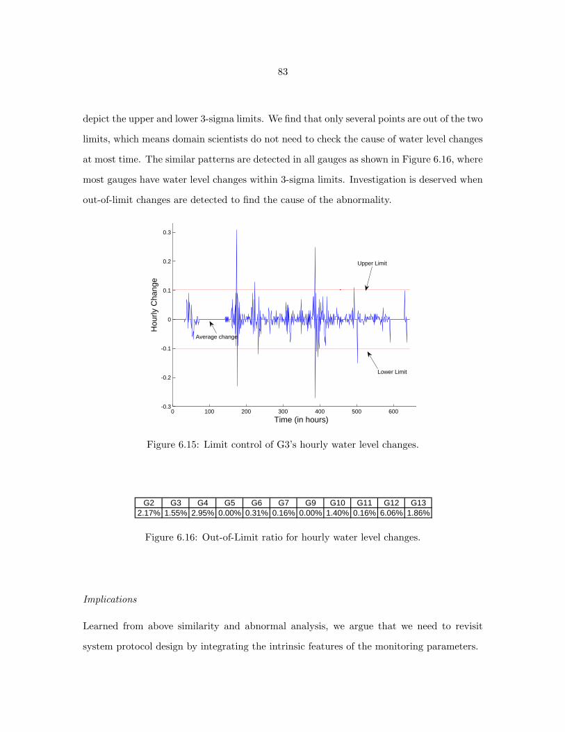
83

depict the upper and lower 3-sigma limits. We find that only several points are out of the two

limits, which means domain scientists do not need to check the cause of water level changes

at most time. The similar patterns are detected in all gauges as shown in Figure 6.16, where

most gauges have water level changes within 3-sigma limits. Investigation is deserved when

out-of-limit changes are detected to find the cause of the abnormality.

0 100 200 300 400 500 600 700-0.3

-0.2

-0.1

0

0.1

0.2

0.3

0.4

Time (in hours)

Hou

rly C

hang

e

Upper Limit

Lower Limit

Average change

Figure 6.15: Limit control of G3’s hourly water level changes.

G2 G3 G4 G5 G6 G7 G9 G10 G11 G12 G132.17% 1.55% 2.95% 0.00% 0.31% 0.16% 0.00% 1.40% 0.16% 6.06% 1.86%

Figure 6.16: Out-of-Limit ratio for hourly water level changes.

Implications

Learned from above similarity and abnormal analysis, we argue that we need to revisit

system protocol design by integrating the intrinsic features of the monitoring parameters.

84

First, we can take advantage of the large amount of data similarity. Because data

similarity is common, it is not necessary to transfer all the collected data to the gateway.

Quality-assured local data processing, aggregation and compression algorithms are necessary

to remove redundant data and reduce overall data volume but keep the quality of the

collected data at a satisfactory level. By enduring a certain level of data inaccuracy, we can

reduce the total amount of collected data up to 90% according to the pattern and numerical

reappearance ratios. In addition, strong patterns are helpful to estimate the future data

and detect abnormal data.

Second, we can use different data sampling rates for different monitoring parameters.

For example, we discover that the changes in voltage is much more frequent than those

in precipitation. Thus, we need to increase the sampling rate to sense voltage data more

frequently, whereas, decrease the sampling rate for precipitation. Furthermore, in the sensor

readings for precipitation, some of them reappear a large amount of times, while others only

appear once. Usually, the readings that only appear once or twice imply a highly dynamic

environment. Therefore, it is better to increase sampling rate so that we can detect the

details in changes.

Third, there may be a lot of abnormal data existing in the sensor reading. Basically, they

can be classified to two categories. One type is transitional, which disappears very quickly.

We can mostly ignore this type of data without affecting overall data quality by replacing it

with a reasonable value. The other type is continuous, which typically lasts a longer period

of time. This type of abnormal data usually implies malicious data or interesting events.

When continuous abnormal data is detected, more attention should be paid to them at the

early stage. For example, more data should be sampled and reported to the gateway as fast

as possible.

Finally, various data sampling rates may result in different amount of data traffic. Sam-

plings for different parameters and detected abnormal data may have different priorities

85

in their delivery to the gateway. A well designed data collection protocol is necessary to

achieve this goal.

6.2.2 Multi-Modality and Spatial Sensing Data Analysis

In the last subsection, we analyzed the similarity and abnormal data for each parameter

individually. In this subsection, we analyze the relationship between two types of sensing

data, water level and precipitation. Moreover, we try to explore the spatial relationship at

different locations.

Gage ID Endurance Interval Confliction ration Endurance Interval Confliction rationG5 (0.00, 0.00)  0.0612 (0.00, 0.01)  0.0408G6 (0.00, 0.00)  0.0263 (0.00, 0.01)  0.0236( , ) ( , )G7 (0.00, 0.00)  0.1778 (0.00, 0.01)  0.1111G9 (0.00, 0.00)  0.0139 (0.00, 0.01)  0G10 (0.00, 0.00)  0.4786 (0.00, 0.01)  0.0679G11 (0.00, 0.00)  0.0476 (0.00, 0.01)  0.0476G12 (0.00, 0.00)  0 (0.00, 0.01)  0G13 (0.00, 0.00)  0.0145 (0.00, 0.01)  0.0145

0.4

0.5

0.6 [0.00, 0.00]

[‐0.01, 0.01]

0

0.1

0.2

0.3

0

G5 G6 G7 G9 G10 G11 G12 G13

Figure 6.17: Conflict ratio of water level and precipitation.

Although water level can be affected by many factors, including moisture when it starts

raining, rainfall intensity, and even temperature and slope of the land, we believe that there

is a relationship between water level and precipitation. Mostly when precipitation increases,

water level should also increase. We count the ratio of the conflict, which is defined as the

appearance when precipitation increases but water level decreases, to verify this relationship.

Figure 6.17 records the conflict ratio between water level and precipitation. In the figure, the

x-axis depicts the gauge ID, and the y-axis shows the conflict ratio. The dark blue bar and

the gray bar denote the conflict ratio with endurance interval [0.00, 0.00] and [−0.01, 0.01]

independently. From the figure we observe that in most cases the conflict ratio is less than

86

6%, which verifies that water level is closely related to precipitation; however, there are two

gauges with conflicts larger than 10%, i.e., G7 has conflict ratio of 18% and G10 has conflict

ratio of 48%. After a carefully examination, we figure out that G10’s high conflict ratio is

related with lots of failures it has. While G7’s high conflict ratio may be caused by other

reasons, because when precipitation increases only a little, other factors, such as moisture

and temperature, may play major roles to determine water level. This is verified by the fact

that when we increase the endurance interval a little, the conflict ratio decreases very fast,

and it eventually disappears when we set endurance interval to [−0.01, 0.01] for water level

and [−0.02, 0.02] for precipitation.

Water Level G2 G3 G4 G5 G6 G7 G9 G11 G12 G13G2 1 0.924 0.174 0.344 0.083 0.314 0.64 0.471 0.513 0.569G3 0.924 1 0.306 0.428 0.254 0.377 0.601 0.505 0.525 0.591G4 0.174 0.306 1 0.486 0.413 0.35 0.35 0.54 0.436 0.528G5 0.344 0.428 0.486 1 0.159 0.916 0.699 0.888 0.875 0.555G6 0.083 0.254 0.413 0.159 1 0.113 -0.1 0.002 -0.01 0.32G7 0.314 0.377 0.35 0.916 0.113 1 0.659 0.832 0.848 0.474G9 0.64 0.601 0.35 0.699 -0.1 0.659 1 0.825 0.835 0.7

G11 0.471 0.505 0.54 0.888 0.002 0.832 0.825 1 0.909 0.627G12 0.513 0.525 0.436 0.875 -0.01 0.848 0.835 0.909 1 0.652G13 0.569 0.591 0.528 0.555 0.32 0.474 0.7 0.627 0.652 1

Figure 6.18: Spatial correlation of water level.

Correlation Coefficients for the same parameter between different gages

Voltage G5 G6 G7 G9 G11 G12 G13G5 1 -0.21 0.004 0.067 -0.54 -0.09 0.15G6 -0.21 1 0.04 -0.23 0.04 0.259 -0.1G7 0.004 0.04 1 0.084 0.013 -0.03 -0.03G9 0.067 -0.23 0.084 1 -0.25 -0.32 0.228G11 -0.54 0.04 0.013 -0.25 1 0.027 -0.27G12 -0.09 0.259 -0.03 -0.32 0.027 1 -0.12G13 0.15 -0.1 -0.03 0.228 -0.27 -0.12 1

Water Level G2 G3 G4 G5 G6 G7 G9 G11 G12 G13G2 1 0.924 0.174 0.344 0.083 0.314 0.64 0.471 0.513 0.569G3 0.924 1 0.306 0.428 0.254 0.377 0.601 0.505 0.525 0.591G4 0.174 0.306 1 0.486 0.413 0.35 0.35 0.54 0.436 0.528G5 0.344 0.428 0.486 1 0.159 0.916 0.699 0.888 0.875 0.555G6 0.083 0.254 0.413 0.159 1 0.113 -0.1 0.002 -0.01 0.32G7 0.314 0.377 0.35 0.916 0.113 1 0.659 0.832 0.848 0.474G9 0.64 0.601 0.35 0.699 -0.1 0.659 1 0.825 0.835 0.7G11 0.471 0.505 0.54 0.888 0.002 0.832 0.825 1 0.909 0.627G12 0.513 0.525 0.436 0.875 -0.01 0.848 0.835 0.909 1 0.652G13 0.569 0.591 0.528 0.555 0.32 0.474 0.7 0.627 0.652 1

Precipitation G5 G6 G7 G9 G11 G12 G13G5 1 0.977 0.996 0.995 0.985 0.996 0.996G6 0.977 1 0.959 0.99 0.996 0.967 0.968G7 0.996 0.959 1 0.983 0.969 0.999 0.998G9 0.995 0.99 0.983 1 0.992 0.988 0.988G11 0.985 0.996 0.969 0.992 1 0.975 0.975G12 0.996 0.967 0.999 0.988 0.975 1 0.999G13 0.996 0.968 0.998 0.988 0.975 0.999 1

Figure 6.19: Spatial correlation of precipitation.

87

We analyze spatial correlation for all of the three parameters. Because there are no

direct communications among sensors at different locations in this application, we do not

expect spatial correlation among voltage readings at the different gauges, which is validated

by the collected data. The calculated co-efficiency value between any two gauges is less

than 0.54 and 99% of them is less than 0.32. However, we do find some spatial correlation

for both water level and precipitation based on the data sensed from various gauges. The

results are depicted in Figure 6.18 and 6.19 retrospectively.

In the figure for precipitation, we only have data for listed gauges. We can see that

all gauges with precipitation data have very large co-efficiency value because they are all

located at LAKE WINNEBAGO, which means that the weather in that area is pretty

uniform. When there is a rain fall at the location of one of the gauges, it is most probably

raining at the locations of the other gauges as well. Water level also exhibits the similar

pattern. In Figure 6.18, gauges located closely usually have high co-efficiency values, which

results in similarity in water level changes, while gauges located far away usually have no

obvious similarity in terms of water level changes. For instance, gauges can be grouped

into several small groups with similar water level changes based on the calculated large co-

efficiency values. Thus, gauge G2 and G3 are within one group with co-efficiency value larger

than 92%. We can see that both of them are located in St. Clair River. G4 is the only gauge

in Detroit River, so it has no high co-efficiency with any other gauges. Moreover, gauge G5,

G7, G11, and G12 show high similarity because they are located closely. Thus, we believe

that geographical similarity exists in the sensed data for water level and precipitation.

Implication

Multi-modality and spatial sensing data analysis helps us to find the correlation between

different parameters and geological correlation of the same parameter. Therefore, data

collected by the correlated sensors can be used as a reference to calibrate the sensing data.

For example, an increase in precipitation mostly results in an increase in water level. When

88

there are some conflicts between them, we need to take a close look and figure out the reason

of the conflict. Furthermore, we can take advantage of similarity in different parameters or

sensors located in different locations. Quality-assured aggregation can be applied in this

scenario to reduce the volume of sensing data. Thus, multi-modality models and spatial

models are very useful in quality-assured data collection protocol design.

89

CHAPTER 7

MODELING DATA CONSISTENCY IN SENSING SYSTEMS

Data consistency models, used as metrics to evaluate the quality of the collected data,

are the core of the Orchis framework. Thus in this chapter, we formally define a set of

data consistency models for different applications. We will first abstract the consistency

related features of wireless sensor networks. Then, we give out the formal definition of our

consistency models. Finally, we propose a set of APIs to manage the consistency.

7.1 Consistency Requirements Analysis

Data consistency is an important problem in computer architecture, distributed systems,

database, and collaborative systems [Peterson and Davie, 2003,Ramakrishnan, 1998,Tanen-

baum and van Steen, 2002]. A lot of consistency models have been proposed in these fields.

However, these models are usually not applicable in WSN because of the specific charac-

teristics of WSN. Thus, consistency models, the key to evaluate the quality of the collected

data, should be remodelled for WSN applications. In this section, we first analyze the dif-

ference between WSNs and traditional distributed systems in terms of consistency; then,

we abstract the data consistency requirements in WSN.

Although a WSN is an instance of a distributed system, there are several significant

differences between WSNs and traditional distributed systems. First, WSNs are resource

constrained systems. Due to the constraints of the memory and the large amount of the

data, the data are usually not stored in sensors for a long period, but they will form data

streams to be delivered to the sinks or base stations. As a result, data consistency in WSN

will not focus on the read/write consistency among multiple data replicas as in traditional

distributed systems; instead, data consistency in WSN is more interested in the spatial and

90

temporal consistency of the same data, i.e., the consistency among several appearances of

the data at different locations and in different time. Second, WSN applications may have

more interests in a set of data which can depict the trends of the monitoring parameter

or report an event by combining these data together. Thus, consistency models for data

streams are more important than those for individual data. In this dissertation, consistency

models for both types of data are modeled. Third, compared with traditional distributed

systems, the unreliable wireless communication is common, rather than abnormal, in WSN.

Although retransmission is a strategy to rectify the effect caused by the unreliable wireless

communication, there is no simple technique that can guarantee the successful delivery of a

message. Thus, in the consistency model, the data loss due to wireless communication should

also be considered. Furthermore, in previous definition of the data consistency [Tanenbaum

and van Steen, 2002], the effect of channel noises and intended attacks are neglected. We

argue that attacks are normal nowadays, and the security technologies should be integrated

in the system design to prevent attacks.

In summary, we conclude that consistency models in traditional distributed systems

that basically discuss the read/write consistency among different replicas are not sufficient

to be applied in WSNs. Given the specific features of resource constraints and unreliable

communication, consistency models in WSN should be remodelled.

Considering both individual data and data streams, we argue that the quality of the data

should be examined from three perspectives: the numerical consistency, the temporal con-

sistency, and the frequency consistency, as shown in Figure 7.1. The numerical consistency

requires that the collected data should be accurate. Here we have two kinds of concerns on

numerical errors: absolute and relative. Absolute numerical error happens when the sensor

reading is out of normal reading range, which can be pre-set by applications. In the case of

absolute numerical error, we can remove it and estimate a reasonable value for it. Relative

numerical error depicts the error between the real field reading and the corresponding data

at the sink. To trade off the resource usage and data accuracy, we can leverage estimation

91

Numerical Consistency

Temporal Consistency

Frequency Consistency

Figure 7.1: A three-dimension view of consistency requirements.

technologies to estimate readings at the sink while still providing the data with the same

level of accuracy. As a result, some sensor readings can be dropped to save resource usage.

Subsequently, there are relative numerical errors between the real ground truth and the col-

lected data at the sink. The temporal consistency means that the data should be delivered

to the sink before or by it is expected. The frequency consistency controls the frequency of

dramatic data changes and abnormal readings of data streams, i.e., the number of dramatic

data changes and the number of readings out of normal reading range in one time interval

should be limited by the application specific consistency requirements. Given this defini-

tion, we can see that the quality of each individual data is determined by the numerical and

temporal consistency, while the quality of data streams is depicted by the combination of

three consistency perspectives.

All these three types of consistency are application-specific concepts, thus different ap-

plication may have various consistency requirements for them respectively. For example,

in a patient monitoring system, emergency conditions of a patient should be reported to

the control panel or caregivers as fast as possible. Otherwise, the patient may be in a

dangerous condition. Thus, most systems that need quick response or have high real-time

92

requirements usually have high requirements on the temporal consistency. Other systems

may have no strict time requirements on the collected data. For instance, a roadside moni-

toring system that counts the number of passed vehicles in one area may only need the data

to be reported twice a day. In this case, data aggregation is more possible because some

aggregation functions need to wait until sufficient data are available. However, these kinds

of systems may have high accuracy requirements (i.e., numerical consistency requirement)

on the collected data. Usually the applications that have high accuracy requirements may

have strict requirements on high frequency requirements for the purpose of quick system

reaction when some abnormal data is detected, e.g., some event-detection applications may

care more on the dramatic data changes and abnormal readings, which usually represent

the occurrence of some interesting events or attacks.

7.2 Consistency Models

We are in a position to propose data consistency models to evaluate the different data

quality. In this section, we first define a general data format used in our models. Then,

we model data consistency for individual data followed by data consistency models for data

streams. Note that we assume that unnecessary data are detected and filtered by detecting

protocols, and an estimation technique [Sha and Shi, 2006a] is used to fill these data at

the sink. In this dissertation, we define consistency as follows. The destination and the

intermediate sensors on the path from the data source to the destination always receive

accurate or meaningful data in a timely fashion.

7.2.1 Data Format

Before we formally model data consistency, we define a general data format that will be

used in consistency models. Considering both the temporal and numerical consistency

requirements and noticing that the frequency consistency requirement is derived from the

numerical values of the data, we define the data format used in consistency models as

93

follows,

(pi, Tstamp, Seq Ran, V al, ReT )

where pi denotes that the data is from the ith sensor for parameter p; Tstamp specifies the

time when the value is sampled and Seq Ran is the range of the sequence number of the

reading at the ith sensor for parameter p. Seq Ran contains only one number where there is

no two continuous readings that have the same value. V al is the value of the reading with

sequential number in Seq Ran, while ReT depicts the remaining time before it is expected

by the sink. The initial value of ReT is set the same as temporal consistency requirements

and the value of Tstmap, Seq Ran, and V al are set locally by the ith node.

As we analyzed in the above subsection, different applications can have various con-

sistency requirements. An example of a consistency requirement is given here, (NE =

0.2,Max T = 3m,Max Diff = 1.2,Max CHG = 5, Range = [1, 4],Max OutRange =

3), where NE = 0.2 means that the application can endure ±0.2 numerical error; Max T =

3m denotes the data should be received at sink in 3 minutes after it is sampled; Max Diff =

1.2 and Max CHG = 5 together define that the number of dramatic changes, the differ-

ence between two continuous readings exceeds ±1.2, should not exceed five; and Range and

Max OutRange requires that the number of readings with value not in the Range should

be less than Max OutRange. These consistency requirements are pre-distributed by other

protocols (Section 7.1). Based on these requirements, we can abstract two consistency se-

mantics: (1) the difference between any two continuous meaningful readings (at the sink)

should be larger than 0.2; and (2) if the number of dramatic changes in one minute exceeds

five, the collected data is not good enough because the detail of the changing is ignored.

Next, we formally model data consistency by using these abstracted semantics. General

ReT should be larger than zero when the data arrives at the sink, all the collected data

satisfy the consistency semantics of the application, specified by the combination of V al and

Seq. The numerical consistency requirements are specified by the consistency semantics,

94

e.g., the application can endure 0.2 error for temperature. In addition, in our consistency

models, we assume the value of the reading is accurate and how to improve the quality of

sensing data is beyond the scope of this dissertation.

7.2.2 Consistency Models for Individual Data

We consider consistency both for individual data and data stream. For each piece of data,

we want to keep the corrected data fresh and accurate, so we will check both tempo-

ral consistency and numerical consistency. Moreover, the consistency can be checked at

different locations and the data may be delivered by various protocols according to differ-

ent application consistency requirements, so we model three types of data consistency, the

hop-consistency, the single-path consistency, and the multiple-path consistency. The hop-

consistency means that the data should keep consistency in each hop, while the single-path

consistency and the multiple-path consistency imply that data consistency holds when the

data is transmitted from the source to the sink using a single path and multiple paths re-

spectively. The hop-consistency is checked at each hop when the data is transferred and it

is maintained if the data packet still has sufficient time to be transferred from current node

to the sink and the value of the new arrive reading is within the range of the consistency

semantics. We define it as below,

HopConsist = (InSemantics(V al, V allast)

&OnTime(ReT, EsTt))−−− (1)

where, InSemantics judges the numerical consistency by checking whether the new arriving

value and the cached last value follow the pre-defined consistency semantics, and OnTime

checks the temporal consistency, i.e., ReT ≥ EsTt denotes that the node has enough time

to deliver the data to the sink. Because the hop-consistency is checked at each hop along

the path, so it is very useful to detect attacks on data and filter redundant aggregated data

95

when data aggregation is applied by using estimation technologies. This will reduce the

source usage while providing the same level of data accuracy.

The hop-consistency defines the consistency only at each hop, however, the end-to-

end consistency between data source and data destination is more important from the

viewpoint of applications. We define this type of consistency as the path-consistency, which

is usually checked at the sink. According to the different routing strategies and application

requirements, we define two types of path-consistency, the single-path consistency using

single path routing and the multiple-path consistency using the multiple-path routing or

flooding. The difference between them lies in that at most one copy of the same data is

reported to the sink in the single-path consistency, while several typically copies of the

same data will be received at the sink in the multiple-path consistency. Both types of path-

consistency consider two concepts, temporal consistency and numerical consistency. We

model the single-path consistency as below,

SPathConsist = (InSemantics(V al, V allast)

&(ReT ≥ 0))−−− (2)

Similar to functions in the hop-consistency, InSemantics checks the numerical consistency

in terms of the consistency semantics. The temporal consistency is reflected by the condition

that ReT is larger than 0 when the data arrives at the sink. In the multiple-path consistency,

several copies of same data will be delivered to the sink. Thus the sink will check the

consistency as k-consistency, which means at least k copies of the same data should be

reported to the sink in time. The multiple-path consistency modeled as below is very useful

to detect the faked readings inserted by malicious nodes (i.e.,fault detection), which might

be very important to some applcaitions.

MPathConsist = (InSemantics(V al, V allast)

&ReT ≥ 0&Count(Pi, Seq Ran) ≥ k)−−− (3)

96

Compared with the single-path consistency, the multiple-path consistency has one more

requirement about the number of copies for the same data, denoted by

Count(Pi, Seq Ran).

7.2.3 Consistency Models for Data Streams

In WSN, data are usually collected in the format of data streams. Individual data may

not have significant meaning, while they are useful when the set of the data are considered

together. Thus, we argue that consistency models for a set of data, data streams, denoted

as D = {d1, d2, ..., dn}, are the same important, if not more important, as the models for

individual data. For data streams, we propose six types of consistency models to satisfy dif-

ferent consistency levels, including the strict consistency, the α-loss consistency, the partial

consistency, the trend consistency, the range frequency consistency and the change frequency

consistency. All these consistency models are taking into consideration of application re-

quirements from three consistency perspectives as analyzed in Section 7.1. The first four

consider the different levels of numerical and temporal consistency while the rest two focus

on the frequency related consistency.

The strict consistency has the most strict requirements to the consistency of collected

data, so it can be used in applications that have extremely high consistency requirements.

To satisfy the strict consistency, three requirements must be satisfied. First, no data is

missed during transmission, i.e., the packet with each sequence number i should be received

at the sink. Second, the temporal consistency is satisfied, i.e., for all received data at the

sink, ReTi ≥ 0. Third, the numerical consistency in terms of consistency semantics is

maintained, e.g., any two continuous readings di and di+1 in the data set D received at the

sink, are out of each other’s endurance range. So the restricted consistency is modeled as

StrictConsist = (InSemantics(D)&∀iReTi ≥ 0

&∀i ∈ [1, n], di ∈ D)−−− (4)

97

The strict consistency differs from the hop-consistency because it is defined based on a set

of data and requires no data lose, so it is stricter than the hop-consistency from this point

of view. Not all applications require the strict consistency, which may be almost impossible

to achieve in a wireless communication based system such as WSN. If we allow some data

loss during transmission, we get the α-loss consistency, where all received data should keep

temporal consistency and at least 1− α percent of totally sampled data should be received

at the sink. So the α-loss consistency can be modeled as

α− LossConsist = (InSemantics(D)&∀iReT i ≥ 0

&Counter(D) ≥ (1− α) ∗max(Seq Ran))−−− (5)

where InSemantics checks the numerical consistency as before. All the received data are

temporal consistent and the number of total received data is large than 1 − α percent of

the number of total sampled data, which is checked based on the sequence number of the

received data. For example,if totally n pieces of data should be received based on the value

of Seq Ran, and the real received number is Counter(D), we can check if the condition in

above formula is satisfied. The α-loss consistency is suitable for applications that have high

real-time requirements. The value of α is adjustable to cater to the numerical consistency

requirements of the applications.

In addition to releasing numerical consistency requirements, we can also release the

temporal consistency requirements, which results in the partial consistency. In the partial

consistency, not all the data are required and the temporal consistency are not so strict,

thus it is modeled as

ParConsist = (InSemantics(D)&∀iReTi ≥ −a

&Counter(D) ≥ (1− α) ∗max(Seq Ran))−−− (6)

98

The partial consistency is similar to the α-loss consistency except that the temporal con-

sistency requirement is released. This consistency model is useful in applications where

aggregation applies, which have numerical consistency requirements but low temporal con-

sistency requirements.

If we further release the numerical consistency requirement, we get another consistency

model named the trend consistency, which is defined as follows,

TrendConsist = (TrendSatisfy(D))−−− (7)

where TrandSatisfy detects if the trend of data streams is maintained. Mechanisms are

needed to evaluate the valid trends. For instance, we might utilize some algorithms from

the signal processing field to evaluate the quality of data streams, e.g., frequency domain

features. This consistency model matches the trend requirement (Section 7.1) of some WSN

applications very well, which could be used in attack-resilient data collection protocols.

Now we consider the abnormal data readings in data collection. In certain applications,

the application scientists may have pre-knowledge of the normal data range of their appli-

cation. This is very helpful to filter erroneous readings, which are resulted from a variety

of reasons, including intended attacks. Also, if the number of abnormal readings exceeds a

certain number pre-set by the application, the application scientists may need to check the

abnormal phenomenon. The notification of the abnormal phenomenon will be triggered by a

violation to the range frequency consistency. Here we define the range frequency consistency

as follows,

RangeConsist = (∀i ∈ [1, . . . , k], Count(Vinot ∈ Range)

< Max OutRange)−−− (8)

where RangeConsist denotes the range frequency consistency. Vi shows a number of k

readings in a time interval and Max OutRange denotes the application pre-set maximum

99

number of readings that may be out of the normal range, Range, in one period. This

consistency can be checked both locally at each sensor and at the sink. Further action are

usually needed by the application scientists when this type of consistency is violated.

In some other applications, application scientists may care a lot about the detail of

the data changes, thus we define the change frequency consistency to detect whether the

changes of the sensor reading are abnormal. The detail of the change frequency consistency

is denoted as follows,

ChangeConsist = (∀i ∈ [1, . . . , k], Count(|Vi+1 − Vi|

> Max Diff) < Max CHG)−−− (9)

where ChangeConsist depicts the change frequency consistency. Vi is a set of total k

readings in a time interval; Max Diff is the pre-set maximum difference between two con-

tinuous readings when the consistency holds, and Max CHG means the maximum number

of dramatic changes, which is defined as the case that the difference between two contin-

uous readings exceeding Max Diff , in one interval. With this consistency, we can either

prevent the data from changing too dramatically or dynamically change sampling rate to

zoom in and observe the details [Sha and Shi, 2006a]. The observation of violation of this

consistency may also result in a request of application scientists involvement.

Moreover, if we consider the spatial relationship among sensed data, we also need to

satisfy the spatial consistency, which is defined as the consistency of the data among geo-

graphically distribution of the data. For example, when we are sampling the temperature,

we may have some pre-knowledge of the geographical distribution of the temperature, thus

spatial consistency should be checked when the data is collected in the sink. Finally, as we

know that there maybe some relationship between parameters, e.g., the speed of vehicles

may correlated with the density of the vehicles on the road, we can further explore the data

relationship among different parameters by defining consistency models for them.

100

In summary, we propose a set of basic but powerful consistency models for data quality

measurement in WSN from the perspective of temporal, numerical and frequency consis-

tency. These models can be used as metrics to evaluate the quality of collected data both

in aggregated format or non-aggregated format. With these proposed basic consistency

models, various applications can find their suitable consistency models for their specific

data quality requirements by adjusting the parameters in these models or composing the

above basic proposed consistency models to form complicated models. For example, the two

frequency consistency models can be combined to control the dramatic data changes and

the abnormal readings in a time interval. The partial consistency and the two frequency

consistency are also composable to set all numerical, temporal and frequency consistency

requirements. Furthermore, various applications should make a trade off between the en-

ergy efficiency and data consistency based on their energy budget, which remains an open

problem in the community.

7.3 APIs for Managing Data Consistency

There is a gap between the lower layer protocols designed to support the consistency goal

and the higher layer consistency requirements from applications. It is critical to provide

user-friend interfaces for application scientists to take advantage of these models. Our APIs

are designed for the purpose of data quality management, and differ from the APIs proposed

in [Welsh and Mainland, 2004]. First, our APIs lie at the higher layer (for application scien-

tists) than theirs (for system programmers). Second, the design goals are different too. We

believe that our APIs can take advantage of theirs in the real implementation. To manage

the consistency, the APIs must have the following functions, checking the current consistency

status (CheckStatus), setting consistency requirements for new parameters (SetReq), updat-

ing consistency requirements (UpdateReq), and getting support from lower layer protocols,

as listed in Table 7.1, where CommPtn denotes the communication pattern to distribute

the consistency requirements; ConMode depicts the name of consistency model. Together

101

with Vreq , Treq and other parameters, ConMode also specifies the consistency semantics;

and Set(n) depicts the set of destination nodes.

Several protocols and algorithms are needed to support the above proposed APIs. For

example, consistency checking algorithms are needed when the CheckStatus API is called.

Various algorithms are needed to check consistency in different models. While in SetReq

and UpdateReq, different protocols are used depending on the size of Set(n). If there is

only one node in Set(n), a point-to-point communication pattern is adopted to deliver the

consistency requirements. When Set(n) contains all the sensors in the field, broadcast is

launched to distribute the requirements. If Set(n) contains nodes located in one area, area

multi-cast is used to disperse the requirements. Hence, various routing protocols are needed

for different communication patterns.

With the APIs we mentioned just now, we can manage data quality of the collected

data based on these models according to application consistency requirements. When the

application needs to sample several different parameters. These parameters have different

consistency requirements; then we can set different models for these parameters, and check

the consistency against these models. For example, in the application of SensorMap [Nath

et al., 2007], we can integrate our APIs with the DataHub in the SensorMap architecture.

When the data arrives at the DataHub, the consistency model is checked. For each data,

suitable consistency model is utilized, so different consistency requirements can be satisfied.

For instance, the k− consistency may be set for accident of alarm data, while ParConsist

is enough for temperature data.

The process of consistency management consists of three steps. First, the consistency

requirements are distributed. Second, the consistency will be checked with support of some

consistency-checking algorithm at the sink after an amount of data are collected. Third,

if the sink finds that current consistency cannot be satisfied because of the constrained

resource, it might release consistency requirements. If the sink find that the quality of

current collected data is not satisfactory, it might increase consistency requirements. These

102

update will be distributed to related nodes, who will in turn change their data collecting

strategy according to the new consistency requirements.

Next, we give an example of how to use these APIs. In a habitat monitoring applica-

tion, if an irregular animal movement is observed in some area, a request to monitoring the

temperature of that area is issued, i.e., SetReq(temp, Set(area), Treq, V alreq, 0, 0, 0, 0, 10%−

LossConsist, area−cast), where temp denotes the name of parameter; Set(area) and area−

cast show that the consistency requirements will be sent to all the nodes in that area using

area−cast. Treq, V alreq and 10%−LossConsist specify the consistency semantics. Four ze-

ros denote no specific frequency consistency requirements. After the application scientist col-

lects some data from the monitoring area, he/she will call CheckStatus(temp, Set(area), last−

one−hour, 10%−LossConsist) to check whether the data received in last one hour satisfy

the requirements specified by the consistency mode, 10%−LossConsistency. Based on the

result of the call, the application scientist makes a decision to tune consistency. For exam-

ple, if the application scientist thinks that the quality of the data is good enough, he will do

nothing to change it; otherwise, he will update the new consistency requirements by calling

UpdateRqe(temp, Set(area), δ(T )), δ(V al), 0, 0, 0, 0, 5%−LossConsist, area− cast). Then,

when receiving the new update request, the node will update the consistency requirements

locally. The whole process forms a close-loop feedback control. In this way, high quality

data could be collected in an energy efficient way.

In this dissertation, we propose to use data consistency as a metric to evaluate the qual-

ity of collected data in wireless sensor networks. In this chapter, several formal consistency

models are defined for different applications. We also propose a set of APIs for the appli-

cation scientists to efficiently manage data consistency. Next, we need to propose a suit of

protocols to provide the system support to achieve the goals in data consistency and energy

efficiency, which are specified by various applications and evaluated by those defined models

in this and last chapters.

103

APIs Function DescriptionsCheckStatus(P, Set(N), Tran, ConMode) Check the consistency of the data from

the nodes in Set(N) during the timeperiod Tran according to the data con-sistency requirements to that data.

SetReq(P, Set(N), Treq , Vreq , Range, Max OutRange, Set the temporal or numerical consis-tency requirements for parameter P tothe set of nodes

Max Diff, Max CHG, ConMode, CommPtn) Set(N) using the specified communica-tion pattern to distribute the require-ments.

UpdateReq(P, Set(N), δ(T ), δ(V ), Range, Max OutRange, Update the temporal or numerical con-sistency requirements for parameter Pat the set of nodes

Max Diff, Max CHG, ConMode, CommPtn) Set(N), and use the specified commu-nication pattern to distribute the up-dating.

Table 7.1: APIs for data consistency management.

104

CHAPTER 8

AN ADAPTIVE LAZY PROTOCOL

The consistency models and lifetime models have been described in previous chapters,

which can be used as metrics to evaluate the energy efficiency property of system protocols

and the quality of the data collected by the wireless sensor system. In this chapter, we

propose an adaptive, lazy, energy-efficient protocol to support achieving the goals of energy

efficiency and data consistency. In the following sections, the protocol will be described in

detail first. Then, the protocol is evaluated in terms of the proposed performance metrics,

both in simulation based on TOSSIM simulator and a prototype using 13 MICA2 motes.

8.1 ALEP: An Adaptive, Lazy, Energy-efficient Protocol

In this dissertation, we intend to save energy by estimating the value of the sensing data

and adapt the data sampling rate to improve the quality of collected data. This in turn will

reduce the number of delivered messages, which is the most significant energy consumption

factor in WSNs [Min and Chandrakasan, 2003], Note that the estimated data should satisfy

the consistency requirements of applications. The objective of this dissertation is to reduce

the number of the delivered message to save energy consumption. In this section, we first

introduce the rationale of our design, then give the details of the protocol.

8.1.1 Rationale

As argued in the previous sections and [Sha et al., 2008a], when the data sampling rate is

low, there will be more estimated data. The sampling rate affect the data accuracy a lot

especially when the estimated value for the data is not so accurate. Estimating data at the

sink is used to save energy but it may hurt data accuracy. There are two extremes between

105

data accuracy and energy-efficiency. For energy-efficiency purposes, we can only gather

and deliver very small amount of data. Subsequently, the gathered data cannot satisfy the

consistency requirements of the application. On the other hand, if we always keep high

sampling rate and deliver a lot of messages to get very accurate data, sensors will run out of

energy very quickly. Thus, we should make a tradeoff between the energy consumption and

the data accuracy. From our observation, we find that the data dynamics varies temporally

and spatially. Furthermore, we also find that it is easier to get accurate estimation when

the data dynamics is low, however it is difficult to get accurate estimation when the data

dynamics is high. Thus, the sampling rate should adapt to the data dynamics in both

temporal and spacial ways. When the data dynamics is high, the sampling rate should be

raised to improve the data accuracy, otherwise, it should be decreased to reduce the number

of delivered energy.

Except adapting the data sampling rate to data dynamics, we can improve the techniques

to estimate the next data, so the number of delivered messages can be dramatically reduced

using estimated data to replace the sensing data and high data accuracy is kept. Besides,

as mentioned in literature [Mainland et al., 2005], sending a message with long length is

more energy efficient than sending several messages with short length. Thus, we intend to

integrate multiple short messages into one big message.

In summary, our proposed Alep protocol consists of three components, adapting the

sampling rate, keeping lazy in transmission based on consistency-guaranteed estimations,

and aggregating and using long length packet. These methods are described in detail in the

following subsections.

8.1.2 Two Types of Data Dynamics

The data consistency should also be integrated with the feature of data dynamics in the

sensor field. In this dissertation, data dynamics means the trend and frequency of data

changes. Usually, the data dynamics comes from two dimensions, temporal data dynamics

106

and spacial data dynamics. In the temporal dimension, data changing frequency varies

at different time periods. Figure 8.1 shows the data changing in terms of the time. In

the figure, the data changes very fast before time t1 and between time t2 and t3, while

it keeps almost stable between time t1 and time t2. Thus, if we keep the constant data

sampling rate, the different data consistency will get during different periods with variant

data dynamics. On the other hand, from the spacial dimension, the data dynamics diffs

from area to area. An example of data changing differing spatially is shown in Figure 8.2.

In the figure, the data changes quickly in the right part of the sensor field and slowly in the

left part. If we use the same data sampling rate in different locations, we will get different

data accuracy, i.e., the collected data may be accurate in the area with low data dynamics,

but not accurate for the area with high data dynamics. Furthermore, the temporal data

dynamics and spacial data dynamics effect the data consistency at the same time. Thus the

data sampling rate should be adapted to the feature of data dynamics from time to time

and from area to area. For example, it should sample more data when the data dynamics is

high and in the area with high data dynamics, while sample less data when data dynamics

is low and in the area with low data dynamics. Moreover, it should use high sampling rate

in the area with high data dynamics and use low sampling rate in an area with low data

dynamics.

8.1.3 Model for Data Dynamics

Before giving the details of the adaptive protocol, we first model data dynamics. To describe

data dynamics, we define a number of windows to observe the data readings. Two param-

eters, winSize and winNum are defined to model the dynamics of data. winSize denotes

the number of readings in one window, e.g., if the winSize is seven, then in one monitoring

window, the sensor will obtain seven readings, winNum specifies the number of windows

in one observation, e.g., if winNum is four, in one observation there will be four windows.

Thus the total number of readings in one observation is Numrd = winSize∗winNum. Since

107

t1 t2 t3

value

Figure 8.1: Data dynamics with the time.

the data dynamics reflects the frequency of data changing, so we first define the frequency

of the data changing as the number of data changing in one observation:

Numchg = {Cnt(i)‖ri+1 − ri| > B&i ∈ [0 : Numrd]}

where, Cnt(i) is the number of is satisfying the conditions; ri and ri+1 are the ith and i+1th

readings separately. B = C(p)bnd is the accuracy bound for this parameter. Based on this

definition, we define the data dynamics (DY N) as the average number of changing in one

monitoring window.

DY N =Numchg

Numrd∗ winSize

From above definition, we can find that the data dynamics is defined based on time

period, i.e., inside the window of observation. By adjusting the value of winSize and

winNum, we can get the data dynamics with various sensitivity. For instance, when we

set winNum small, the value of DY N will be calculated with high frequency, i.e., it can

be very acute to the data changing. While the value of winSize controls the range of the

DY N , e.g., if we set winSize to two, data dynamics can be expressed as above one and

108

Figure 8.2: Data dynamics in different location.

below one; however, if we set the value of winSize to four, data dynamics can have four

levels, below one, one to two, two to three, and above three. Based on data dynamics, it

is possible for users to choose suitable data sampling rate to accurately collect data in an

energy efficient way, which will be explained in detail in Section 8.1.

For a series of n sensing data, if we get every piece of data, the accuracy is the best

by using reading values as estimation values. If we get readings in a half frequency, the

accuracy will decrease since we have to estimate half of the data. On the other hand, the

energy is saved from sampling and reporting less data. Thus data sampling rate should

be decided by making tradeoff between the data accuracy and energy efficiency, which, we

argue that, can be achieved by matching data sampling rate to data dynamics. Because

data sampling rate should fit data dynamics, we model the behavior of data dynamics here.

The dynamics of the data stream can be viewed as two dimensions, temporal and spatial.

For example, in the dimension of temporal. Figure 8.1 shows the data reading changing in

terms of the time of the same sensor. In the figure, before the time t1 and between time t2

and t3, the data changes very frequently, while it keeps almost stable between time t1 and

time t2. An example of data changing differing from different location at the same time is

109

shown in Figure 8.2. In the figure, we can see that the data changes quickly in the right

part of the sensor field and it changes very slowly in the left part in the figure. Thus for

accurately collecting data in an energy efficient way, the data sample rate should be adapted

from time to time and from area to area. For example, it should sample more data when

the data dynamics is high, while sample less data when data dynamics is how. Similarly, it

should use high sample rate in the area with high data dynamics and use low sample rate

in an area with low data dynamics.

8.1.4 Adapting the Sample Rate

Figure 8.3: Adapting data sampling rate.

We adapt the sampling rate based on the model for data dynamics defined in previous

sections. The process of adapting the sampling rate is a process of reinforce learning [Sutton

and Barto, 1998] based on the data reading as shown in Figure 8.3, i.e., the data is sampled

based on the current sampling rate; then the data dynamics is calculated; finally, the data

sampling data is adjusted to fit the data dynamics. In the model, data dynamics reflects the

average number of changes in one monitoring window. Thus based on the value of DY N ,

we can define the adaption of the sampling rate as

Rsmp =

dDY N−Avechg

Dfbnde ∗Rcr, DY N > Avechg

Avechg−DY NDfbnd

∗Rcr, DY N ≤ Avechg

110

where, Rsmp is the adapted sampling rate; Rcr is the current sampling rate. Avechg is the

normal average changes happen in one window size; and Dfbnd bounds maximum difference

between the observed value of data dynamics and the normal average changes, i.e., if DY N is

larger than Avechg and the difference exceeds the bound, the sampling rate should increase;

when DY N is much smaller than Avechg, the sample rate should be decreased.

Based on this formula and the figure, the sampling rate learns from the previous data

dynamics, and uses the most recent data dynamics to estimate the future data dynamics.

The data history is limited by the number of windows and the window size in one observa-

tion. The result of adaption divides the sample rate to several levels based on the value of

bound, and find a suitable level for the future data collection. By adjusting the length of

history based on the window size and the number of windows, we can adjust the frequency

of sample rate changing and the acuteness of the changing of the environment, e.g., we can

change the sampling rate very quickly by setting small value to the number of windows in

observations.

8.1.5 Keeping Lazy in Transmission

One way to reduce the number of delivered messages is to keep lazy in transmission, i.e.,

only sending the messages that are necessary to be sent. We think that if the receiver can

estimate an accurate enough value for the current reading, the message need not to be sent,

i.e., if the data consistency requirement can be hold, the messages is not necessary to be

sent.

In this protocol, every sensor caches the last reading for every parameter for all potential

senders that may deliver message to it, and it uses the cached values as the estimation of

the current reading. To check the data consistency for this piece of data, the sensor will

use the current reading as the real value and the cached value as the estimated value. If

the difference between the current reading and the cached value is within the consistency

bound, the sender will not send this piece of data, i.e., keeping lazy. For example, in an

111

application which monitors the temperature of a sensor field, when a sensor gets a reading

of value 3.7, and the cached last reading is 3.5 which is within the consistency bound of 0.3.

So the new reading is not necessary to be sent. When the current data reading is absent,

the sensor assumes the value is unchanged so that it keeps silent.

In the case of the aggregated data, every receiver caches a copy of the latest aggregated

value calculated from senders. After it applies the aggregation function, it will compare the

new calculated value with the cached value. If the difference between them is within the

consistency bound, the sender will keep silent. For the aggregated data, the receiver has to

wait for the new reading from all the senders for a period of time. If there are still data

absent from some senders, the receiver will use the cached data to substitute the current

reading and calculate the aggregated value.

8.1.6 Aggregating and Delaying Delivery

Another aspect of the lazy approach is to integrate several pieces of data into one message to

reduce the number of message. However, we still need to keep the timeliness for the data. In

our application, the expected time to deliver the message to the sink can be estimated based

on the number of hops to the sink. For example, if we assume it takes Tdev to transmit one

message from the child to the parent, then we can estimate the time it takes from current

sensor to deliver a message to sink is Tdev × Hjs, where Hjs is the number of hops from

the current sensor to the sink. Then the time bound for the data is the sum of the current

estimated time plus one time slot, which denotes the time between two reporting points

according to the TDMA schedule. Using the estimated time to the sink, we can easily check

the temporal consistency requirement for the parameter.

8.1.7 Discussions

Note that the proposed protocol is a general protocol for sensor networks, we still have

several assumptions. First, the data readings from sensors are accurate, i.e., here we do not

112

consider reading errors. Second, synchronization between sensors are kept by using some

mechanisms, e.g., RBS [Elson et al., 2002]. Third, sensors in the sensor field are static,

which is true in most monitoring-based applications. Finally, the sensors in the sensor field

are homogeneous, i.e., each sensor has the same physical capacity.

Although our protocol is proposed for a tree-based sensor network, the basic idea of

adapting the data sample rate, keeping silent during transmission and merging transmissions

can be applied in any protocol to achieve both the data accuracy and energy efficiency. In a

tree-based sensor network, this protocol can be implemented by an ideal TDMA schedule.

From the model for the problem definition, we can see that the optimization at a single

sensor can guarantee the system level optimization. However, the system level optimization

doesn’t necessarily require the optimization at single sensor. The consistency requirement

at a single sensor is more rigorous than the consistency requirement for the whole sensor

network. So, we may loosen the consistency requirement for individual sensor a little, and

the consistency requirement for the whole sensor network will still be hold at a very high

probability.

In our design, we use the last reading to estimate the previous reading which is consistent

when the transmission is reliable. However, it only reduced the messages having data within

the consistency bound, when the current reading of the data is in the endurance bound of

the real reading. If other techniques that can accurately estimate the value of the data

out of the range of the consistency bound, it will further reduce the number of delivered

messages, which will be our future work.

8.2 Performance Evaluation: Simulation

To evaluate the performance of the proposed protocol, we have implemented the protocol in

TinyOS using the TOSSIM [Levis et al., 2003] environment and compared with two other

protocols, Simple which is a TDMA-based data collection protocol and Lazy which only has

the lazy feature of the proposed protocol. In the rest of this section, we will describe the

simulation setup and the performance metrics first, followed by the performance evaluation

113

in simulation environment. The results of a prototype implementation and evaluation is

reported in the following section.

23 Mobile and Internet Systems LaboratoryCSC8260 Project

0

4

321

5

120

6

Figure 8.4: A tree-structured sensor network used in the simulation and prototype. Thenumbers next to each node is node ID or Mote ID.

8.2.1 Simulation Setup and Evaluation Metrics

In our simulation, 121 nodes are connected forming a four layer complete tree, as shown in

Figure 8.4, where all the internal nodes have three children and the root acts as the sink.

The sensors periodically collect data from its children and report the readings to its parent

based on a TDMA schedule. Besides, the sensors may have the ability of aggregation. The

data consistency requirements at each sensor are preloaded from the sink by broadcast. The

whole circle area is divided into three sub-areas, which is covered by a sub-tree. Each sensor

node acts as a multiple functional sensor, which can sample three parameters: Temperature

as Temp, Pressure as Press, and Rain-index as Humid. To evaluate the proposed protocol in

different data dynamics environments, we intentionally make these three parameters have

different dynamic characteristics. For example, the reading always changes faster for Temp,

relatively stable for Press, while medium for Humid. To simulate spatial data dynamics, we

intentionally separate the whole area into three sub-areas with different data dynamics as

114

shown in different colors (gray levels in B/W print out) in the figure. The reading changes

faster in the left subtree area, relatively stable in the right subtree area, and medium in the

middle subtree area.

For the perspective of spatial, the reading of each parameter will differ based on the

location. Basically, in our simulation, the whole area is separated to three sub-areas as

shown in Figure 8.4, where the data changing in the area covered by the left subtree is always

fast, while slow in the area covered by the right subtree, and normal in the area covered

by the middle subtree. Three algorithms will be simulated in our experiment. First, the

method without considering both lazy and adaptive approaches will be simulated, denoted

as Simple. Second, the method with lazy approach but without adaption is simulated,

denoted as Lazy. Finally, the method considering both lazy and adaptive approaches is

simulated, denoted as Alep, where we try to keep α−Consistency where α = 20. The

consistency is checked at each sensor as well as the base station.

The goal of the Alep protocol is to save energy by reducing the number of delivered

messages while satisfying the data consistency requirements. Thus, we use three metrics to

evaluate our approach. To measure the energy efficient property, we count the total number

of delivered messages and the dropped voltage at each sensor (in prototype evaluation), and

to examine the tradeoff between the energy efficiency and data consistency. Thus, Alep will

be examined in three ways: Does this protocol reduce the number of the messages and extend

the lifetime of WSN? Does this protocol improve the accuracy of data? What is the tradeoff

between the number of delivered messages and the data accuracy? To answer the question

of the effect of reduced messages to data consistency, we propose a new performance metric

called data inconsistency factor (DIF), which is defined as the total variance between the

gathered data in the sink and real data, i.e., V =∑n

1 (drcv − dfld)2, where, V is the value of

variance; drcv and dfld are the reading value received at the sink and the real value sampled

at the data field respectively. The more accurate the data, the smaller the variance.

115

To examine the tradeoff between the energy consumption and the data accuracy, we

adjust the value of the temporal consistency bound and the numerical consistency bound,

which are two parameters in the Alep protocol. By adjusting these parameters, we can

get different simulation results in terms of energy consumption and data accuracy. we will

adjust the parameters in the Alep protocol to show the effect of these parameters to the

energy consumption and data accuracy. These parameters includes the bound of both time

accuracy and value accuracy.

8.2.2 Number of Delivered Messages

Usually collecting more data is a way to improve the data accuracy; however, by adapting

the sampling rate to fit the feature of data dynamics and keeping lazy when data is in

the range of consistency, data accuracy can be improved without significantly increase the

number of delivered messages. Moreover, in some cases when the data dynamics is low, the

data consistency can be kept even by delivering less number of messages. In this section,

we show the number of messages delivered at each sensor using different approaches.

Figure 8.5 lists the number of delivered messages at each sensor without and with aggre-

gation respectively. The x-axis is the ID of each sensor, and the y-axis denotes the number

of delivered messages. Note that the y-axis of Figure 8.5 (a) and 8.5 (b) are at different

scales. As a matter of fact, the number of delivered messages for all approaches reduces

significantly when aggregation is used. From the two figures, we can see that Simple gen-

erally delivers the most number of messages and Lazy transfers almost the least number of

messages in both cases of with and without data aggregation. That is because Lazy filters

a lot of unnecessary messages.

These three approaches have totally different performance in terms of the number of

messages delivered. In the case of without data aggregation shown in Figure 8.5 (a), the

sensors are classified to four types based on the layer in the tree using Simple, i.e., sensors

in the same layer using Simple delivers the same number of messages. However, using Alep

116

and Lazy, the sensors transmit different number of messages because of the variant data

dynamics in the different areas. For example, among sensors located at layer 3, sensors

with ID between 13 and 21 transfer 140 messages because the high data dynamics of the

monitoring area, while the sensors with ID between 31 and 39 only deliver 41 messages

because the low data dynamics of the monitoring area, which is less than 13 of that in

the high dynamics area. The similar results exist in the case with data aggregation in

Figure 8.5 (b), where all the sensors deliver the same number of messages using Simple,

while the sensors using Alep and Lazy located at different areas transmit different number

of messages, i.e., the sensors located at high dynamics area deliver 57 messages but the

sensors located at low dynamics area only send 9 messages, which denotes that Alep does

adapt the data sampling rate to the dynamics of the data

Comparing with Lazy, we observe that the sensors using Alep send more number of

messages than using Lazy at the area with high data dynamics (e.g., node 13 – 21) but send

less number of messages than that of using Lazy at the area with low data dynamics (e.g.,

node 31 – 39). This is because the sampling rate is increased considerably in the area with

high data dynamics and decreased a lot in the area with low data dynamics. From above

analysis, we conclude that Lazy can always reduce the number of delivered messages, and

Alep usually does not increase the number of delivered messages and reduce the number of

delivered messages a lot when the data dynamics is low.

To take full advantage of adapting sample rate, we need an intelligent adaptation scheme,

which is our future work. In the following sections, we will see that reducing of the number

of messages does not necessary degrade the consistency of the collected data.

8.2.3 Data Inconsistency Factor

From above sections, we can see that Lazy and Alep can largely reduce the number of deliv-

ered messages. However, delivering less message means that there are more data estimated

at the sink, which may result in the degradation of the data consistency. In this subsection,

117

0

500

1000

1500

2000

2500

20 40 60 80 100 120

Num

ber

of m

essa

ges

Node ID

Alep-no-aggrLazy-no-aggr

Simple-no-aggr

Figure 8.5: Number of delivered messages without aggregation.

we examine the effect of unsent messages to the data accuracy. We use data inconsistency

factor as the metric to measure the effect.

We use the data inconsistency factor to evaluate the quality of the collected data. Fig-

ure 8.7(a) reports the relationship between the data inconsistency factor and different mon-

itoring parameters with variant data dynamics. In the figure, the x-axis is different data

types with variant data dynamics and the y-axis represents the calculated data inconsistency

factor of the collected data. Three types of parameters with different data dynamics are

monitored, among which Temp has relatively higher data dynamics than Humid and Press,

while Press has relatively lower data dynamics. Furthermore, for each parameter, data

dynamics also varies according to different areas, i.e., each parameter has three types of

data dynamics, high, high first then low denoted as mix, and low. Thus, there are totally

nine sets of data with variant data dynamics.

In the figure, we note that when the data dynamics is higher, the value of data incon-

sistency factor is larger, e.g., the Temp high has a larger data inconsistency factor than

118

10

20

30

40

50

60

70

80

20 40 60 80 100 120

Num

ber

of m

essa

ges

Node ID

alep-aggrlazy-aggr

simple-aggr

Figure 8.6: Number of delivered messages with aggregation.

Temp mix and Temp low, and Temp high also has a larger data inconsistency factor than

Humid high and Press high. The reason is that when the data dynamics is high, it is

more difficult for the sink to estimate the correct data. From the figure, we also find that

Alep has much smaller data inconsistency factor than that of Simple and Lazy when the

data dynamics is high, while it has larger data inconsistency factor than that of Simple and

has the same data inconsistency factor as Lazy when the data dynamics is low. This result

shows that Alep indeed makes the sampling rate fit the feature of data dynamics, i.e., when

the data dynamics is high, it will use higher sampling rate to gather more data so that to

make the variance small. Otherwise, it will sample less data to save energy.

Furthermore, the data inconsistency factor increases very fast with the increasing of data

dynamics using Simple and Lazy, but increases slowly using Alep. As a result, Simple and

Lazy may not collect enough accurate data when the data dynamics is high, i.e., the data

inconsistency factor exceeds the data consistency requirements of the application. However,

Alep can keep the data inconsistency factor low by adapting the data sampling rate to data

119

Figure 8.7: Data inconsistency factor.

dynamics. We should also notice that Alep improves the data accuracy meanwhile somehow

reduces the number of delivered messages as shown in Section 8.2.2.

Comparing Lazy with Simple in terms of the accuracy of the collected data, Lazy has very

close value of data variance as Simple, however, in Section 8.2.2 we know that Lazy delivered

less messages than Simple, which means that the dropped messages are not necessary to be

transferred to the sink. Thus, we conclude that lazy delivering can reduce the number of

delivered messages, while the approach of adapting the data sampling rate to data dynamics

can significantly improve the data accuracy. It is good to integrate those two approaches to

collect accurate data in an energy-efficient way.

8.2.4 Tradeoff between Energy Efficiency and Data Consistency

We have already seen that Lazy and Alep can largely reduce the number of delivered messages

so that they have potential to save energy and extend the lifetime of WSN, and Alep can

120

0

20

40

60

80

100

120

20 40 60 80 100 120

Num

ber

of d

eliv

ered

mes

sage

s

Nodes ID

temporal bound 4temporal bound 5temporal bound 6temporal bound 7

Figure 8.8: Number of messages with variant temporal bound using Alep.

sufficiently improve the data consistency. Now we are in position to examine the effect

of two key factors related with Alep: the temporal consistency bound and the numerical

consistency bound.

The performance of Alep is largely decided by the two key factors, the temporal consis-

tency bound and the numerical consistency bound. Here we study the effect of these two

factors.

First let us consider the effect of the temporal consistency bound to the energy efficiency

and data numerical consistency. If we release the temporal consistency of data, the same

set of data will be delivered to the sink regardless of different arrival times. Thus changing

the temporal consistency bound will not affect the data inconsistency factor of the collected

data. However, releasing the temporal consistency bound does affect the number of delivered

messages. Figure 8.7(b) displays the relationship between the number of delivered messages

and the different temporal consistency bounds ranging from 4 units to 7 units, which is

the maximum time to transfer a message to the sink assuming each hop taking one unit

121

time. In the figure, the x-axis is the ID of the sensors and the y-axis is the number of

delivered messages. From the figure, we can see that the increasing of the bound of temporal

consistency results in the decreasing of the number of total delivered messages. When the

temporal consistency bound is tight as 4, some sensors deliver more than 110 pieces of

messages because data combination is not possible. While the temporal consistency bound

is raised to 7, sensors deliver only about 50 pieces of messages. Thus, releasing the bound

of temporal consistency can reduce the number of delivered messages. However, based on

simulation data, the energy consumption almost keeps the same (overlapped in the figure)

with the releasing of the bound of the temporal consistency as show in Figure 8.8. This

is because the same reason of idle listening. Subsequently, this will reduce the energy

consumption. In this case a well designed schedule is needed to save energy from idle

listening. This problem may be solved automatically in the new version of Motes, such as

TelosB [Polastre et al., 2005], which can automatically transfer to the sleeping state.

0

20

40

60

80

100

120

140

20 40 60 80 100 120

Num

ber

of d

eliv

ered

mes

sage

s

Nodes ID

value bound 0value bound 1value bound 2value bound 3

Figure 8.9: Number of messages with different numerical consistency bound.

122

0

200

400

600

800

1000

1200

1400

1600

1800

2000

0 0.5 1 1.5 2 2.5 3

Dat

a in

cons

iste

ncy

fact

or

Value bound

Temp-highTemp-mixTemp-low

Humid-highHumid-mixHumid-lowPress-highPress-mixPress-low

Figure 8.10: Data inconsistency factor with variant value bound using Alep.

Having seen that releasing the temporal consistency bound can reduce the number of the

delivered messages, next, we examine the effect of the numerical consistency bound to the

number of delivered messages and the data inconsistency factor. We also examine the effect

of the numerical consistency bound. Figure 8.9 shows the number of delivered messages

with the relation to the variant value constraints. In the figure, the x-axis is the ID of the

sensors and the y-axis shows the number of delivered messages. From the figure, we can

see that when the numerical consistency bound is enlarged, the number of the delivered

messages is decreased very fast. Next, we examine the changing of data inconsistency factor

with the changing of the numerical consistency bound. Figure 8.10 shows the relationship

between the data inconsistency factor and the value of the data consistency bound. The

x-axis is the different value bounds and the y-axis depicts the value of the data inconsistency

factor. In the figure, when the data consistency bound is released, the data inconsistency

factor increases very quickly, especially when the data dynamics is high. Thus we argue

that there is a tradeoff between the data consistency and the energy efficiency. Releasing

123

the data consistency bound results in both energy efficiency and larger data inconsistency

factor, so the application should decide the data consistency bound based on its specific

data consistency requirements. If the application cares little to the data consistency, it may

raise the bound, otherwise, it has to use a tighter bound.

5

10

15

20

25

30

35

40

45

50

55

60

20 40 60 80 100 120

Num

ber

of d

eliv

ered

mes

sage

s

Nodes ID

nummsg-max4nummsg-max8

nummsg-max16nummsg-max32nummsg-max64

Figure 8.11: Number of delivered messages with variant maximum data sampling rate.

Besides the temporal consistency bound and data consistency bound will effect the

variance and the energy efficiency. Another factor, the maximum data sampling rate will

also affect these two performance. Here we check the effect of the maximum data sampling

rate, which is the maximum data sampling rate Alep may take. Figure 8.11 denotes the

number of delivered message with different variant maximum data sampling rate. In the

figure, the x-axis is the ID of the sensors and the y-axis shows the number of delivered

messages. We can find that the maximum sampling rate will not affect the number of

delivered messages a lot. Only when the sample rate change to very small, it will sample

more data when the data dynamics is low.

124

8.3 Performance Evaluation: Prototype

Although the simulation results have shown the advantage of Alep and Lazy, we further

evaluate them in a prototype implementation, where energy consumption is measured more

directly and accurately. In the prototype, 13 MICA2 Motes form a tree similar to that in the

simulation except that it has only two layers, the root of the tree is connected to a desktop.

Other configurations of each sensor is the same as that in the simulation. Each Mote

samples three parameters with different data dynamics and the whole tree is divided into

three subareas with various data dynamics. For comparison purposes, three algorithms are

implemented, including Alep, Lazy and TinyDB, a simplified version of TinyDB [Madden

et al., 2005] without data aggregation.

In the implementation, we find that the program developed for TOSSIM could not

be executed at MICA2 Motes directly because TOSSIM does not enforce the same strict

memory constraints as that in MICA2 Motes. However, to compare these three protocols,

we need to feed them enough data, either synthesized or real traces, to show the differences.

This is a challenge in the prototype implementation because we cannot use the data sampled

from the sensor board directly. As a substitution, trace based approach and a data generator

are considered. However, we argue that the trace based data feeding does work in sensors

smoothly. First, it is impossible to hold a long trace in the program flash memory of tiny

sensors, which have only 128k bytes in total. Second, there are also some disadvantages

to store the trace file at the measurement flash of MICA2, which has 512k bytes in total.

For example, as denoted in [Shnayder et al., 2004], the current for reading MICA2 sensor

board is 0.7mA, while the current for reading and writing EEPROM is 6.2mA and 18.4mA

separately. These overheads are comparable with that for receiving and sending messages.

Thus, a lot of energy will be consumed by reading data from measurement flash so that

the energy consumption of the protocol cannot be accurately evaluated. Furthermore, the

total possible access time of the measurement flash is limited [Shnayder et al., 2004]. So,

we decide to design a data generator for evaluation purposes. In our prototype we decide

125

to design a data generator to produce the same set of data as the sampling feedings for all

protocols. The detail of the data generator is described as next subsection.

8.3.1 SDGen: Sensor Data Generator

δiOOC kk +=+11 ?

δiOOC kk −=+13 ?

kk OOC =+12 ? kk OOC =+12 ?

δiOOC kk −=+13 ?

δiOOC kk −=+13 ?δiOOC kk +=+11 ?

δiOOC kk −=+11 ?

δiOOC kk +=+11 ?

kk OOC =+12 ?kk OOC =+12 ?

Figure 8.12: State transition diagram of sensor data generator.

We intend to design a general sensor data generator, SDGen, which can be used by other

researchers for evaluating their protocols and algorithms as well. SDGen is a simple data

generator based on the a finite state machine as shown in Figure 8.12 (a), which intends

to generator the same series of random readings. In the figure, the four circles denote the

four states. SDGen remembers the latest output as Ok and a state as one of the four circles

in the figure. To generate a new sampling, it first generates a random number. Based

on the value of the random number, the conditions, C1, C2, and C3, are checked and the

state of the machine is transferred. The action after the satisfied condition is executed and

an new output Ok+1 is produced based on Ok. For example, if C1 is in the range of [0.0,

0.9], and the random number generated is 0.6, then Ok+1 = Ok + δ is the output and the

126

machine transfer state from 1 to 2; if C2 is in the range of (0.9,1.0], and the random number

generated is 0.95, then the output is Ok+1 = Ok and the machine state is not changed.

Our SDGen has several advantages. First, it is very easy to implement and it only needs

to remember the last state and the last output, which reflects the fact that the next sampling

is usually closely related with the latest previous reading. Of course, we can make it more

complicated by remembering more previous readings. Second, the same set of random data

can be generated if we fix the value of the random seed, which satisfies our requirements

of feeding the same set of data to all protocols. Actually, in our implementation, we find

that it is important to keep the order of the generated random number, because we need

to gradually generate samplings for three parameters. We take the following strategy in

our implementation: all samplings are read from a short array, which stores a set of latest

generated data and the order of the generation is controlled by the length of the array.

Third, SDGen can generate sampling series with different data dynamics by adjusting the

parameters, including the value of i and the condition Ci. For instance, if we make C2

to be in [0.0, 0.8], which means that any two continuous samplings are the same with a

probability of 80%, dynamics of the generated data will be very low, while if we make C2

to be in [0.0, 0.1], dynamics of the generated data will be much higher.

8.3.2 Comparison Number of Delivered Messages

As argued in [Min and Chandrakasan, 2003], the number of delivered message dominates the

energy consumption in WSN applications. Thus we first compare the number of delivered

messages using these three protocols. As hinted in [Sha and Shi, 2004,Sha and Shi, 2005],

the lifetime of a WSN is decided by a set of communication intensive sensors, which are layer

one nodes in a tree-based structure. Thus, we compare the number of delivered messages

of these layer one nodes only.

Figure 8.12(b) shows the results of number of delivered messages. In the figure, the

x-axis is the Mote ID, which also depicts the area with specific data dynamic feature and

127

0

20

40

60

80

100

120

140

160

180

200

1 2 3

Mote ID

TinyDB Lazy Alep

Figure 8.13: Comparison of number of messages delivered by Layer one Motes.

the y-axis is the number of received messages at the sink from the corresponding Mote. We

find that in all cases, both Alep and Lazy send much less number of messages than TinyDB.

For example, when data dynamics is high, TinyDB sends about 170 messages, while Alep

and Lazy send only about 100 messages. When data dynamics is low as for Mote 3, TinyDB

still sends about 170 messages, but both Alep and Lazy send less than 30 messages. With

the gradual decreasing of data dynamics from Mote 1 to Mote 3, TinyDB sends almost the

same number of messages, while both Lazy and Alep send less messages. Compared with

Lazy, Alep sends comparable number of messages in all cases; however, it sends a little more

messages when data dynamics is high, and sends a little less messages when data dynamics

is low. This denotes that Alep does adapt the data sampling rate to match data dynamics.

8.3.3 Comparison of Energy Consumption

We use the voltage drop to show the energy consumption in these three protocols as shown

in Figure 8.14, where the x-axis is the Mote ID and the y-axis is the value of the initial and

final voltage read from every node using different protocols. The initial voltage is measured

128

2.85

2.9

2.95

3

3.05

3.1

3.15

1 2 3 4 5 6 7 8 9 10 11 12Node ID

Volts

InitialTinyDBLazyAlep

Figure 8.14: Comparison of voltage dropping of different protocols.

before the protocol is executed and the final voltage is measured after 50,000 samples are

collected. We use the same brand new AA Alkaline batteries in all the experiments to get

the same initial voltage, 3.138 volts, and we find that different protocols result in different

final voltages. TinyDB consumes much more energy than the other two. For example, the

voltage drops 0.24 volts at layer one nodes and 0.22 volts at layer two nodes in TinyDB,

while it drops only 0.20 and 0.18 volts correspondingly in both Lazy and Alep. As expected,

layer one nodes consume more energy than layer two nodes because they need to forward

messages for the latter. Motes in the same layer consume similar energy. The areas with

different data dynamics consume almost the same amount of energy, because the number

of messages does not differ too much; however, we still see that the area with lowest data

dynamic does consume less energy than the Motes in other areas. Lazy and Alep have very

close energy consumption, however lazy consumes less than Alep, especially for the layer

one nodes. In summary, we find that the energy consumption mostly matches the result of

129

the number of delivered messages. Alep and Lazy are really energy efficient, and they can

extend the lifetime of WSNs considerably.

8.3.4 Comparison of Samplings

Comprison of Samplings (TinyDB vs. Real)

626466687072

1 6 11 16 21 26 31 36 41

Sampling serial number

Comparison of Sampling (Lazy vs. Real)

626466687072

1 6 11 16 21 26 31 36 41

Sampling Serial number

Comparison of Sampling (Alep vs. Real)

626466687072

1 6 11 16 21 26 31 36 41

Sampling serial number

Comparison of Samplings (TinyDB vs. Real)

555759616365

1 6 11 16 21 26 31 36 41

Sampling serial number

Comparison of Samplings (Lazy vs. Real)

555759616365

1 6 11 16 21 26 31 36 41

Sampling serial number

Comparison of Samplings (Alep vs. Real)

555759616365

1 6 11 16 21 26 31 36 41

Sampling serial number

Comparison of samplings (TinyDB vs. Real)

182022242628

1 6 11 16 21 26 31 36 41

Sampling serial number

Comparison of samlings (Lazy vs. Real)

182022242628

1 6 11 16 21 26 31 36 41

Sampling serial number

Comparison of samplings (Alep vs. Real)

182022242628

1 6 11 16 21 26 31 36 41

Sampling serial number

(a) High dynamics area (b) Regular dynamics area (c) Low dynamics area

Figure 8.15: Comparison of received data at the sink with real data. Note that the SQUAREshape represents the values of real data and the DIAMOND shape shows the value ofcollected data.

We have shown the energy efficiency property of Alep. Next we want to show that Alep

can also improve data quality. The most intuitive way to show the quality of collected

data is to compare them with the corresponding data generated by SDGen, acting as real

data. In this experiment, we sample every 4 readings from all data generated by SDGen in

TinyDB and Lazy, and the sampling rate is changing in Alep because of adaptation. Other

three readings will be estimated as the same as the sampled one.

In Figure 8.15, three types of data with variant data dynamics are shown with the x-axis

denoting the sampling serial number and y-axis depicting the value of the corresponding

130

sampling. The figures should be read column by column. When data dynamic is high as high

as with a probability of 90% to change, as show in Figure 8.15(a), all three protocols perform

similar at the beginning, but Alep catches the trend of the sampling better than the other

two protocols because it adapts to a high sampling rate. Thus more details are observed, for

example, between sampling serial number 21 and 40, Alep catches the dynamics of the data

very well, while both Lazy and TinyDB miss the details. Furthermore, Lazy filters more

details than TinyDB, but we argue that the degrading of data quality will not be significant

because it is bounded by the consistency endurance range of Lazy. In Figure 8.15(b), data

dynamics is not as high as that in (a) by setting the data changing probability to be 60% in

SDGen. All three protocols collect very similar data, which captures the dynamics of real

data. In this case, although Alep seems not perform better than TinyDB, it delivers much

less messages than TinyDB. Moreover, we can adjust the parameter in Alep so that the

adaptation can be sharper, e.g., we can set small window size and decrease the threshold of

adaptation. Alep can capture more details of the data changing. The data collected from the

low dynamic area is shown in Figure 8.15(c), where we observe that all three protocols can

capture the trends of the sampling very well. However, Alep catches the trend a little later

than TinyDB and Lazy, because Alep decreases the sampling rate when the data dynamics

is low. As a result, some immediate changes are ignored and postponed to next time when

the data is sampled. This will not be a problem if we set the minimum data sampling rate

close to the regular data sampling rate in TinyDB. Comparing Lazy with TinyDB, we find

that they are mostly comparable, especially when the data dynamic is not very high, so we

can save a lot of energy by using Lazy.

8.3.5 Comparison of Data Inconsistency Factor

We have seen the advantage of the Alep protocol directly and intuitively from the sampled

data readings. We also want to compare these protocols quantitatively in terms of data

inconsistency factor as shown in Figure 8.16, which the results for three layer one nodes

131

Mote 1 Mote 2 Mote 3 TinyDB Lazy Alep TinyDB Lazy Alep TinyDB Lazy Alep High dynamics 772 748 678 495 783 409 517 515 629

Mixed dynamics 558 498 610 205 309 341 532 658 624 Low dynamics 116 346 354 87 187 229 136 234 546

Figure 8.16: Comparison of data inconsistency factor.

only. From the figure, we can see that the result is close to that in simulation. When

data dynamics is high, Alep can reduce data inconsistency factor, but while data dynamics

is low, Alep increases data inconsistency factor a little. However, we argue that we can

control the increasing of data inconsistency factor by limiting the minimum sampling rate

during adaptation, from which we still can get the advantage of reducing a large amount

of messages. Furthermore, data inconsistency factor will be much less if we think the

data within tolerance range as consistent in the calculation of data inconsistency factor.

Compared with Lazy, Alep has larger data inconsistency factor when the data dynamics is

very low, because Alep neglects a lot of details by decreasing the sampling rate.

8.3.6 Discussions

In summary, from both simulation and prototype evaluation, we find that Alep can improve

data quality when the data dynamic is high and reduce the number of delivered messages

a lot in almost all cases. We also find that the minimum sampling rate is very important

to control the quality of collected data, which decreases very fast if the sampling rate is too

low to get the details of data changing. Releasing the temporal consistency requirements

is helpful to reduce the number of delivered messages so that to save energy, as well as

to decrease the probability of communication collision and increase the possibility of data

aggregation, so we expect less package loss rate in Alep and Lazy than that in TinyDB.

However, it may also make the messages piled and exceed the limitation of the total memory

of MICA2. Thus, we should set a low bound for temporal consistency requirements.

132

We also realized that trace-based approaches only work in the simulation but fail in the

prototype test due to the memory constraints. Compared with TinyDB, Lazy and Alep may

have more strict requirements on the correct delivery of the messages because the effect of

data loss will be more severer than that in TinyDB. Retransmission strategy may be applied

here. Furthermore, TinyDB’s optimization when message queue is full can also be applied

in Alep and Lazy, however, we argue that the probability that message queue is full in Lazy

and Alep is much less than that in TinyDB because the number of total delivered messages

is significantly reduced. Finally, the performance of Alep can be improved by tuning the

parameters, which deserves further investigation.

133

CHAPTER 9

D4: DECEPTIVE DATA DETECTION IN DYNAMIC SENSINGSYSTEMS

We envision that the successful of wireless sensing systems is determined by the quality

of the collected data, and the quality of the collected data is mainly affected by the deceptive

data, which usually comes from two sources, wrong readings resulted from inaccurate sensing

components and unreliable wireless communication, and false data inserted by malicious

attackers. Thus the major concern to improve the data quality is to detect and filter

deceptive data. The problem of how to improving data quality have been studied in several

previous efforts, such as security approaches and reputation based approaches, but we argue

that those approaches are necessary to improve the quality of the collected data, while they

are not sufficient to attack the problem of data quality management, especially in a highly

distributed highly dynamic environment such as vehicular networks.

In this dissertation, we intend to propose a general framework to detect the deceptive

data from the view point of data itself. Basically, we try to filter two types of deceptive

data, redundant data and false data. In our framework, those two types of deceptive data

are treated differently. Quality-assured aggregation and compression (Section 9.2) is used

to detect and filter redundant data, while role-differentiated cooperative deceptive data

detection and filtering (Section 9.3) and self-learning model-based deceptive data detection

and filtering (Section 9.2) are utilized to filter false data. Finally, when both types of

deceptive data are checked and recognized after the data are delivered to a central server,

a spatial-temporal data quality checking can be performed to further detect and filter the

remaining deceptive data. The novelty of our approach exists in two-fold. First, to the

best of our knowledge, we are the first to propose a general framework in deceptive data

134

detection and filtering, and we are the first to propose role-differentiated deceptive data

detection and filtering.

Among the several mechanism to detect and filter deceptive data, in this dissertation,

we focus on the role-differentiated deceptive data detection and filtering mechanism, and we

apply this mechanism in the scenario of a dynamic wireless sensing system called vehicular

network, which is composed by a large amount of vehicles with sensing, computation and

communication functions. The basic idea of role-differentiated deceptive data detection and

filtering is described as follows. First, the vehicles in the system are classified into several

groups, road side unit (RSU), public vehicles such as police cars, school cars, and normal

vehicles. Each group plays different roles and has different impacts in checking the reported

data. For example, in such a system, both RSU and public vehicles have higher trust level

than normal vehicles if an event is reported or confirmed by them, and by take advantage

of some physical parameters, a vehicle credits most to its owe observation to the event.

The reported event will be regarded as false report when there is no sufficiency information

about the report is confirmed, thus it will be filtered by the system. In this way, we detect

and filter false reports and deliver the legitimated reports as fast as possible.

The rest of this section is organized as follows. Section 9.1 shows the necessary to detect

and filter deceptive data in new ways, which is followed by the design of a general framework

to detect and filter deceptive data in Section 9.2. Among the several mechanisms proposed in

the framework, we give detailed description of the role-differentiated cooperative deceptive

data detection and filtering mechanism in Section 9.3. Section 9.4 describes an application

of the proposed mechanism in vehicular networks.

9.1 Necessity of Deceptive Data Detection and Filtering

A lot of wireless sensing system applications have been launched in last several years, in-

cluding habitat monitoring, environmental monitoring, acoustic detection, and so on. Fur-

thermore, vehicular networks and healthcare personal area sensing systems become widely

applied recently. Among those applications, The major function of the sensing networks

135

is to collect meaningful and accurate data. In those wireless sensing system applications,

two types of data are mostly interested, sensed readings of monitored parameters such as

temperature in the room, and detected events like an appearance of the enemy. According

to the feature of actions to those collected data, we classify them into two main categories,

emergency data and regular data. When the emergency data is collected and reported, a

followup action should be taken to take care of the detected event in a prompt way. For

example, in a high performance computing system, if it is detected that the temperature

of one node is too high, we may have to move workload from this node to others as soon

as possible. While regular data, which usually has no restrict timeliness requirements, can

be all the sensor readings about the monitoring parameters except those emergency read-

ings. Although those two types of data have different features, they share some common

requirements in terms of deceptive data detection and filtering.

9.1.1 Deceptive Data Definition

In this dissertation, we classify the deceptive data into two categories, redundant data and

false data, based on the affect of the deceptive data to the performance of the sensing

systems. The redundant data is defined as the data that shares the exactly same or very

similar information with data reported in previous time slots or by other nearby sensors.

Most redundant data should be detected and filtered because of following reasons. First, as

specified in [Sha and Shi, 2008], in most cases removing redundant data will not degrade the

quality of collected sensing data. Moreover, a lot of redundant data will ruin the performance

of sensing systems. For example, redundant data will increase the communication, storage

and computation overhead when they are transferred from the sensors to the sink. In this

case, a lot of limited resources are wasted. Even worse, if the network traffic and storage are

occupied by these deceptive data, a lot of meaningful data have to be delayed in transmission

or even dropped because of running out of storage, thus the quality of the collected data

will be largely degraded. Therefore, it is necessary to filter the redundant data and save

136

resources to deliver more important data. On the other hand, these redundant data provide

us replicated information, which is very helpful in building a fault-tolerant sensing system.

Thus, there is a tradeoff on detection and filtering these redundant data. We argue that

we will adapt our redundant data detecting and filtering protocol to the requirements of

sensing system applications, which will decide the redundance level of the collected data

that is needed for fault-tolerant purpose.

Another type of deceptive data are false data, which may result from the following sev-

eral sources. First, false data may be caused by the malfunction of the sensor board so that

wrong sensor readings are generated. Second, due to the unreliable wireless communication

and limited resources in wireless sensing networks, data may be lost or changed in trans-

mission because of collision. Finally, because of the limited capability in providing high

level security and adverse deployment environment of the sensors, sensors may be captured

and compromised easier than regular computers. As a result, these compromised sensors

can insert false information to raise malicious attacks. False data will degrade data qual-

ity in two ways. On one hand, false data is similar to redundant data in that it occupies

limited resources and increases the probability of dropping meaningful data. On the other

hand, things can be even worse because false data can bring diaster to the sensing system

applications. For instance, false data can directly affect the quality of the collected data in

that it increases the data inconsistency factor defined in [Sha and Shi, 2008]. Furthermore,

false data can cause wireless sensing system in malfunction. For example, wrong traffic

information can direct drivers to take some paths with high traffic but avoid some paths

with low traffic. In some worse cases, the false data like an emergency brake notification

in vehicular networks may result in more severe consequences such as collisions. Thus, it

is critical to detect and filter false data as much as possible to avoid the disasters it may

bring.

137

In this dissertation, we are more interested in detecting deceptive data in highly dynamic

systems, because in such systems, the sensing nodes behavior changes fast resulted from a

variety of reasons, necessitating a quick-response and filtering mechanism.

9.1.2 Insufficiency of Previous Approaches

Security technologies using traditional cryptography mechanisms, such as encryption for

confidentiality, hashing digest for message integrity, are employed. However, we argue that

these technologies are necessary in detecting and filtering deceptive data but they are not

enough in detecting deceptive data, because of mostly they are trying to prevent attackers.

Follows are several reasons. First, most of those security based approaches try to prevent

attackers, but they rarely check the data themselves. To be specific, they try to validate

the legitimation of the reporting nodes, but not validate the legitimation of the value of the

reported data. Thus, if the attacker is from legitimate but compromised nodes, it is very

difficult for them to detect and distinguish the attacker from a normal reporter. Second, in

mobile sensing systems that have high mobility, there is no permanent relationship between

any two sensor nodes, so it is very difficult to verify each other by using the traditional

security strategies like mutual authentication. In addition, the extreme large scale of the

system and high mobility put a big challenge in key distribution if a security based approach

is adopted. Finally, in such a totally distributed environment, all decisions should be made

locally. Without the help of a central server, the deceptive data is detected only based on

partial local information, which makes the problem more difficult. The difficulty is increased

when the decision have to be made in a real-time way.

Besides security technologies, reputation based approaches, which usually require strong

identity, cannot work in this case because of the possible large scale, the highly dynamics,

and lack of the help of a center server in the system. Several other previous efforts have

also been made in deceptive data detection and cleaning; however, most of them assume

a specific distribution of the monitoring parameter, and they use this distribution as a

138

model to predict and check the reported value of monitoring parameters. These methods

can be useful techniques to detect deceptive data, but they rely a lot on the correctness of

the distribution, so they cannot be generally extended to many applications. In summary,

we find that deceptive data detection and filtering is the key to improve the quality of

the collected data and the performance of dynamic sensor systems. With the insufficient

of previous solution, it is essential to propose novel effective solutions to detect and filter

deceptive data.

9.2 A Framework to Detect Deceptive Data

It is necessary to clean deceptive data to improve the system performance of wireless sensing

systems. In this section, we design a framework, D4, to detect and filter deceptive data, as

shown in Figure 9.1. shows the components in the framework, A total of four mechanisms

are proposed in the D4 framework to detect two types of deceptive data as much as possible,

in which, we propose four mechanisms to detect and filter deceptive data. Some mechanisms

can be used in detecting and filtering both deceptive data, while some of them are specifically

designed for only one type of deceptive data, either the redundant data or the false data.

From the figure, we can see that the process of deceptive data detection consists of two

steps. The first step is done locally at each sensor that gets access to the data, when the

data is sampled or received during transmission, and the second step is executed at the

sink, when a lot of data has been delivered to the sink. At the first step, three detection

mechanisms are defined, including quality-assured aggregation and compression, self-learning

model-based detection, and role-differentiated cooperative deceptive detection and filtering,

among which we think that the self-learning model-based detection can be used to detect

and filter both types of deceptive data, although the parameters in the model may be

adjusted to achieve a optimized result. Quality-assured aggregation and compression and

role-differentiated cooperative detection are devised for detecting and filtering redundant

data and false date independently. After all data arrive at the sink, the second step is

conducted. A general spatial-temporal data quality check will be applied to check the

139

Deceptive Data Detection and Filtering

Redundant Data False Data

Quality-assured Aggregation and

Compression

Role-differentiated Cooperative Detection

and Filtering

Self-learning Model-based

Detection and Filtering

Systematically Spatial-temporal Data Quality Checking and Recognition

Figure 9.1: An overview of the framework to detect and filter deceptive data.

consistency of the all collected data. Next, we give an overview of these four detection and

filtering mechanisms one by one.

9.2.1 Quality-Assured Aggregation & Compression

Quality-assured aggregation and compression is designed to detect and filter redundant

data. It trades off the amount of delivered data with the quality of the collected data as

well as fault tolerance. This mechanism works as follows. First, the quality requirements of

the monitoring parameters are pre-set at each sensor. Second, when the data is collected at

each sensor, the sensor starts to process data aggregation and compression when necessary.

In this case, due to the constraints of storage and communication bandwidth, the maximum

amount of data that each sensor can store and send is limited. When the collected data

does not exceed this limitation, the sensor stores all new coming data. When the sensor

runs out of resource, but it senses or receives more new data, it will start the process of data

aggregation and data compression. We define a similarity factor to represent the level of

deference between two pieces of data. During the aggregation, two temporally continuous

140

sensor reading with maximum similarity factor will be aggregated by removing one piece

of sensor reading. This process continues until the amount of remaining data is within

the storage limitation. Quality-assured aggregation and compression are very useful to be

applied to filter redundant data, because each time the filtered data lose least information

compared with others. Thus when the maximum amount of sensed data and the size of

the available storage is fixed, the quality of the collected data can be assured with a high

probability using our quality-assured aggregation and compression.

9.2.2 The RD4 Mechanism

Role-differentiated cooperative deceptive data detection and filtering is devised to confirm

the correct event reports and thus to prevent false event reports. In this mechanism, each

sensing node is assigned a role, with corresponding right to confirm an event. When an event

is detected at one sensor, the sensor starts to collect the confidence score of this event. The

event will be confirmed and sent to other sensors when the confidence score exceeds a preset

threshold. Otherwise, the event report will be dropped when confidence score expires after

some time. When the event report is receive at another sensor, it will follow the same

process to confirm and propagate the event report. The detail of this protocol is described

in Section 9.3.

9.2.3 Self-Learning Model Based Detection

Self-learning model based detection and filtering is a mechanism to detect and filter both

redundant data and false data. In this mechanism, models should be carefully defined to

evaluate the legitimation of the collected data. Basically these models will explore the locally

spatial-temporal relationship among the collected data by taking advantages of physical

features of the sensing data. Because the decision will be made locally at each sensor or on

the path from the data source to the sink, the models should be designed under the condition

of limited storage and computation, as well as partial information. In most applications, the

141

detection and filtering algorithm is also required to be real-time, because redundant data

has to be dropped immediately to reduce resource usage and false data that will result in

wrong system functions has to be filtered as early as possible to avoid disasters. To achieve

this goal, we define some consistency models, which consists of a set of rules to check the

quality of the collected data. To be efficient, these rules will be simple, so the overhead

of the consistency checking based on these rules can be controlled. Also, the rule set is a

flexible set, which may increase or be modified based on the experience of the sensors. If

the collected data can pass the checking of the rule set, we regard it as not deceptive data,

otherwise, it will be detected as deceptive data and be filtered. We adopt a self-learning

mechanism to manage the size of the rule set. At first, only basic rules will be defined to

check the consistency of collected data. With the sensors getting more experience in the

data collection, the rule set can be extended. For example, if a piece of false data is not

detected by sensor A, but it is detected and confirmed by other sensors, sensor B, after

sensor A is informed this missing detection, it can modify the rule set by adding new rules

or changing the parameter in the current rule. Thus, next time, when this type of false data

arrives at sensor A, sensor A can detect it with a high probability.

9.2.4 Spatial-Temporal Data Recognition

After the data is collected at the sink, a systematically spatial-temporal data quality check-

ing and recognition is executed. Because the sink is usually much more powerful than

other sensors, more complicated consistency checking operations can be processed. With a

large amount of data available at the sink, the spatial-temporal relationship among sensor

readings can be examined based on pre-defined consistency models. For example, based

on the analysis of the previous collected sensing data, we can abstract some distribution of

the monitoring parameters. Thus, if one piece of the collected data is far away from the

distribution, it must be a piece of false data. Moreover, although we try to filter redundant

data, there will still be spatial redundant data because sensors’ monitoring field may overlap

142

and an event can be detected and delivered by several sensors independently. We observe

that those redundant data usually exhibits a certain type of similarity, i.e., they are close

in the value or reporting a similar event. In general, this type of redundancy offers us a

chance to verify the legitimation of sensing data by mutual verification. Finally, we argue

that several monitoring parameters may have relationships among them. For instance, the

detected vehicle speed is closely related with the density of the vehicles on the road. When

a vehicle reports a high driving speed and another sensor reports a high density of traffic,

most probably there will be false reports, i.e., either the vehicle is reporting a false speed or

the density of the traffic is not so high. We should take advantage of the relationship among

different parameters so that we can model this type of features, and use those models to

detect as well as filter more false data which is not able to be detected and filtered locally

during the data is sensed and transmitted due to the availability of only partial information,

limited computation and storage resources.

9.2.5 Discussion

Deceptive data detection and filtering is a challenge in wireless sensing system design. The

framework we proposed in this dissertation provides four general mechanisms to achieve

the goal of deceptive data detection and filtering; however, as we have known that wireless

sensing systems are mostly application specific systems. Thus, for specific wireless sensing

system applications, we need to give details of each suitable mechanism and adapt our mech-

anism to satisfy the specific application requirements in detecting and filtering deceptive

data so that the deceptive data can be detected and filtered with a high probability. We

argue that it is very difficult to guarantee detecting and filtering all deceptive data, but we

can make efforts in increasing the probability that these data is detected and filtered. In

this framework, we totally introduce four mechanisms, but we will only give details of the

RD4 mechanism and leave the rest of them as our future work.

143

9.3 Role-differentiated Cooperative Deceptive Date Detection and Filtering

Among the four proposed mechanisms to detect and filter deceptive data, in this dissertation,

we try to address one of them in detail, which is the RD4 mechanism . In this section, we

describe the detail of the mechanism as follows.

In the mechanism of role-differentiated cooperative deceptive data detection and filtering

(RD4), when a sensor is deployed, it picks up a role from the role set based on the specific

features of the sensor, such as storage size, computation ability, communication ability,

and trustable level, which specifies how much can this type of sensor be trusted. Then,

each sensor plays a different role in the system and has the functions assigned to that role.

The role set of a specific wireless sensing system application can be pre-defined as R =

{R1, R2, R3, ..., Ri}. For each event it sensed or received, the sensor can issue a confidence

score to the event, which is denoted as csr(E, T )ij , denoting the truth level of this event,

where E specifies the event, and i and j are the identity of the role and the identity of the

sensor independently, while T means the score will be valid for T time slots. We define the

maximum confidence score that a sensor with ID j and role Ri can issue to a piece of data

or an event report as CSR(E, T )ij , which should satisfy csr(E, T )ij ≤ CSR(E, T )ij .

In the RD4 mechanism, whenever an event report is generated or received at a sensor,

the sensor will check whether it is a false event or not. Thus, an event report will be checked

the whole way from location it is detected to the sink of that event. Next we give details

on how to set the confidential score and how to detect and filter a false event.

In RD4, the confidential score defined above is calculated based on the accumulated

signal strength during a certain time period ([0, T0]), depicted as ASS(E, T0)ij , of the

corresponding event E at sensor j with role i. Here, the signal strength of an event E,

denoted as SS(E)ij , can be defined as the amount of changes of a monitoring physical

parameter within a unit time period. For example, if we try to detect an event of sudden

changes in temperature at a computing node in a high performance computing system. The

signal strength will be the amount of temperature changing within each minute. Of course,

144

for different types of application, the signal strength can be defined in different ways based

on the special physical parameters. Thus, if the function to specify the changing rate of a

monitoring physical parameter is p(t), we can define SS(E)ij as

SS(E)i,j = p(t)dt

Based on the defined SS(E)ij , the accumulated signal strength can be defined as

ASS(E, T0)ij =∫ T0

0SS(E)ij =

∫ T0

0p(t)dt

Having the ASS(E, T0)ij , we design a function f that maps the accumulated signal

strength to a confidential score, to be specific, csr(E, T )ij = f(ASS(E, T0)ij). When an

event is detected at a sensor, the sensor will set up a timer T , also used as the first lifetime

period of the event, to the detected event. Then the sensor will try to confirm where it is a

really event or just a faked one before the event expires. The decision is made based on the

confidence score of the event, which can come from two sources. One is the observation by

the sensor itself, for which we use accumulated signal strength detected by the senor, and

the other is the reported signal strength about the same event from other sensors. Then the

sensor j assigns a confidence score, csr(E, T )ij , to the detected event, E, within a lifetime

of T as follows.

csr(E, T )ij = f(ASS(E, T0)ij)

=

ASS(E, T0)ij ASS(E, T0)ij ≤ CSR(E, T )ij

CSR(E, T )ij ASS > CSR(E, T )ij

Based on the above formula, if the calculated confidence score exceeds the bound which

is pre-set by the application to confirm an event. The sensor that detects the event will

generate an event report and broadcast the event report to all other sensors in the sensing

systems. The event report, denoted as R(E), is a five tuple, including the information

145

about the signal strength of the event, the first lifetime period of the event, event ID, event

detector ID and the role of the detector. Thus, we have R(E) = (AAS(E, T0)ij , T, E, j, i).

Note that T is the lifetime of the event and T0 is the latest timestamp when the event

is seen. With the event ID and the detector ID, the event can be uniquely determined.

Otherwise, the sensor will wait to collect more confidence score within the lifetime of the

event, or drop the event when the event expires. When the event report is propagated, the

report will be received by other sensors. If we assume the kth sensor receive a set of event

reports from its N neighbors, we can calculate the accumulated signal strength for event E

as follows.

ASS(E, T0)rk =N∑

n=0

Wjn ∗ASS(E, T0)jn +∫ T0

0SS(E)rk

where ASS(E, T0)lk depicts the accumulated signal strength of the event E at sensor K

with role r, which consists of two parts, the aggregation of received signal strength of event

E from other sensors, denoted by ASS(E, T0)jn, and the accumulated signal strength based

on its own observation at sensor k. Wjn is the weight of the event report from sensor n. It

can be defined as the reverse of the distance between two sensors, the similarity of the two

events detected by the two sensors, the trustable level of the sensor n, or the importance of

the sensor n to sensor k. We argue that the definition of the weight should be adaptive to

the nature of different sensing systems applications as well as requirements of the sensing

systems applications.

Having the calculated accumulated signal strength, we can calculate the confidence score

at sensor k. Based on the confidence score, we can make a judge on the truth of the

event. That is to say, If the confidence score exceeds the pre-set bound to confirm the

event, the event is confirmed and a new report about this event is generated and forwarded.

Otherwise, it will wait another T more time period to check the accumulated signal strength

and calculate the new confidence score again. Considering the timeliness of events, in our

146

design, the signal strength will degrade with the time passing. Thus, at the end of each T

time period, signal strength recalculated based on the following formula.

ASS(E, T0 + T )rk = αASS(E, T0)rk

+N∑

n=0

Wjn ∗ASS(E, T0 + T )jn +∫ T0+T

T0

SS(E)rk

In the above formula, ASS(E, T0 + T )rk depicts the accumulated signal strength at

sensor k against event E at the time T0 + T . α is the degrading rate of the signal strength.

Thus, in the formula, the first part is the degraded signal length observed before time T0,

and the second part is the received accumulated signal strength from other sensors between

time T0 and time T0 + T ; while the third part is the accumulated signal strength observed

by sensor k in the time interval [T0, T0 +T ]. The event will be regarded as a false event after

it is checked twice but does not confirmed yet. In other words, the event will be discard if

it cannot be confirmed within 2T . Based on the confidence score, a final judgement on the

truth of the event is generated as follows.

V alid(E) =

True csr(E, T )ij > θ||csr(E, 2T )ij > θ

False otherwise

This formula means that the event is confirmed as true when confidence score exceeds

a pre-set threshold; otherwise, the event is confirmed as false and the propagation of the

event report will be terminated. In this way, we can image that the true event will be

propagated very fast and it will be dropped after a while either because the farther sensor

cannot detect the event or not so many sensor are sensing the reports. Thus, we can control

the propagation of the event within a reasonable big area. If the event is a faked event,

then it will have very little chance to be confirmed and propagated, so the faked events can

be controlled within a very small area.

147

We argue that waiting 2T periods to confirm a reported event has advantages over just

waiting one T period. First, if we only wait T period to confirm the even5, some true

event may be dropped very earlier because not enough signal strength has been collected,

which will be true in a highly distributed sensing environment with only insufficient local

information. Of course, we can wait several time intervals of T to get enough strong signal

strength; however, because the event report has timely features, the signal strength will

degrade after some time the event is detected and reported. In this case, the number of

waiting period, nT , should be controlled and the degrading of the signal strength should

be taken into consideration as well. Finally, some wireless sensing applications have high

real-time requirements, so we cannot make the waiting period too long.

In this section, we propose a general mechanism, role-differentiated cooperative detection

and filtering, for sensing systems to detect and filter false data, especially false event reports.

Because variant sensor network applications have their own features, our mechanism should

be adjusted to fit the application requirements of specific applications. In this dissertation,

we try to verify the effectiveness and efficacy of our mechanism in a dynamic sensor network

environment, thus we use a vehicular network as an example to test our mechanism. In the

next section, we give details about how to use our mechanism to detect and filter deceptive

data in the context of vehicular networks.

9.4 RD4 in Vehicular Networks

We propose a general mechanism using role-differentiated cooperative approach to detect

deceptive data. We argue that our mechanism can be applied in a lot of applications, how-

ever, we will only evaluate the efficiency and efficacy of our mechanism in one application,

which is a dynamic sensor network. As we have pointed out in previous section, our mecha-

nism should be adjusted to satisfy application requirements of different applications. In this

section, we give an example of how to adjust our role-differentiated cooperative deceptive

data detection mechanism in a vehicular network application.

148

The RD4 mechanism is a general mechanism to detect deceptive data. In this section,

we adapt the RD4 mechanism to detect false accident report in the context of vehicular

networks.

9.4.1 Role Definition in Vehicular Networks

In this subsection, we define a detailed role-differentiated false accident event detection

protocol in vehicular networks. The first step to define the RD4 mechanism is to define

a set of different roles in vehicular network applications. Considering different types of

function components such as vehicles and road side units (RSUs) in vehicular networks, we

classify those function components to four roles, including RSUs, public vehicles such as

police cars, school buses and so on, regular vehicles like personal owned cars, and vehicle

itself. Thus the role set in the vehicular networks is defined as R = {Rrsu, Rpub, Rreg, Rself}.

For each role Ri, it can assign a maximum confidence score, CSRij , to an accident report

it detests or confirms based on the characters of the role. In our design, the definition of

maximum confidence score (CSR) is closely related the trustable level of each role in the

vehicular network. For example, we think that RSUs are more trustable than all vehicles

that are on the road because of two reasons. First, they are mostly controlled by public

organizations such as Department of Transportation (DoT) or some certificated companies,

thus it is more difficult for attackers to compromise these devices. Moreover, because the

RSUs have more power in terms of computation, storage and communication, fixed-location

deployment and relatively high availability, they usually have more information than other

vehicles. As a result, RSUs usually reports more accurate data than other on-road vehicles

so that they have higher trustable level, thus they can issue bigger value of confidential code

and send out stronger signal strength. Comparing the public vehicles with regular vehicles,

we argue that public vehicles have more protection than the regular ones, e.g., police cars

are equipped with high security devices and always managed by police department, so

public vehicles are more creditable than regular personal owned vehicles. Except those

149

three regular roles, we have another special role, Rself , in our system, for which we believe

that it should have the highest trustable level. Thus, we define the CSRijs following the

order of CSRself,j > CSRrsu,j > CSRpub,j > CSRreg,j .

9.4.2 False Accident Report Detection

In this dissertation, we assume that the detection of a true accident is handled by the

accident sources, which can either be the vehicles that are involved in the accident or the

police cars that are taking care of the accident. This assumption is based on the following

observations. When an accident happens, thought the vehicle will be damaged, even totally,

not all parts in the vehicle will crash. For example, in most cases when an accident happens,

at least two tires of the vehicle will still be in a good condition. Thus, the sensors equipped

on the those two tires can initialize an accident report and propagate it to other passing

vehicles. On the other hand, the accident report can also be initially generated by police

cars. In most cases, when an accident appears, a police car will come to the site where

the accident appears very soon. Except those two types of vehicles, other vehicles are not

supposed to report an accident. In other words, any accident reports generated by vehicles

except above two type are false accident reports. Malicious vehicles may insert false accident

report by performing as the vehicles involved in the accident. Thus, our goal is to remove

false accident reports from malicious vehicles. In this dissertation, we assume that each

vehicle is equipped a tamper-proof component, so even if a vehicle is compromised, it still

cannot generating multiple identities.

When an accident report is received by a vehicle on the road. The vehicle will make a

judgement about the truth of the accident report, based on the signal strength from its own

observation and the signal strength reporting the same event from other vehicles. In our

design, based on the reality that traffic will be blocked so that the vehicles will slow down

when an accident happens. We use the vehicle velocity deceleration as the signal strength

defined in the model. Thus p(t) = a(t) = dv/dt, where a(t) is the acceleration rate, and v is

150

the velocity of the vehicle. Then, the signal strength observed by vehicle j, ASS(E, T0)ij ,

can be calculated as ASS(E, T0)ij =∫ T0 a(t) = vT −v0 = ∆v. To emphasize the importance

of roles, we assign important role a special ability to send out accident reports with stronger

signal strength, thus after we calculate the accumulated signal strength observed by the

vehicle itself, we will adjust the accumulated signal strength by considering the role of the

vehicle. The new accumulated signal strength we get is

ASS(E, T0)ij =CSR(E, T )ij

CSR(E, T )reg,j∆v

Except the signals strength gained from the observation of the vehicle j, vehicle j will

receive signal strength for the event E from other vehicles. If we integrate both types of

signal strength of the event E, we get an integrated value of the accumulated signal strength

of event E at vehicle j with timestampe T0 as follows.

ASS(E, T0)ij =N∑

n=0

Wjn ∗ASS(E, T0)jn

+CSR(E, T )ij

CSR(E, T )reg,j∆v

Similarly, we can calculate the integrated value of the accumulated signal strength after

a period of T time slots, which is specified as following.

ASS(E, T0 + T )ij = αASS(E, T0)ij

+N∑

n=0

Wjn ∗ASS(E, T0 + T )jn +CSR(E, T )ij

CSR(E, T )reg,j(vT0+T − vT0)

Having calculated the integrated value of the accumulated signal strength, we can map

it to get a confident score for the event E at the vehicle j using the same function we define

in Section 9.3.

Considering the fact that an accident on the road will only affect the vehicles close the

the area where the accident is detected, we give more weight to an accident report that is

151

from a location closer to the accident. Also, we argue that reporting of accident is more

trustable for the vehicles located closer to the sources, since the vehicles located closer to

the source is more likely to observe the accident than farther ones. Thus we define the value

of Wjn as the reverse of the distance between the location of reporting vehicles and the

location of the accident source, i.e., Wjn = 1dst(n,a) , where dst(n, a) specifies the distance

between vehicle n and the accident.

Based on the value of the confident score, we can make a judgement on the truth of

event E at vehicle j. If the accident is confirmed as a true accident, it will be propagated

by sending a message from vehicle j, including the event report, ASS(E, T )ij , T, E, i, j,

where ASS(E, T )ij is the signal strength of the event E, while i and j is the role and the

identity of the vehicle independently. Otherwise, the accident report will be dropped. For

different vehicle roles in the networks, we may also assign different values of threshold. For

example, the threshold of the RSUs will be higher than that of regular vehicles, because

RSUs are more powerful than regular vehicles and they have more effect on the decision

making than regular vehicles to other vehicles in the network.

9.5 Performance Evaluation

We are in a position to evaluate the effectiveness and efficiency of our proposed protocol. In

this section, we will first describe a vehicular network simulator. Then, we will evaluate our

protocol in terms of several performance metrics, namely recall, accident report propagation

range, accident report confirmation time, respectively in the rest of the this section.

9.5.1 Simulation Setup

We design a simulator for vehicular networks, by extending the traffic simulator designed

in [Thiemann et al., 2008,Traffic Simulator, ] that simulate the movements, such as accel-

eration, decrepitation, exchange lane, of the vehicles. We simulate the RD4 mechanism for

vehicular network in a road segment of a two-lane one way highway scenario with a ramp

where vehicles enter the highway. We extend the simulator is the following three ways.

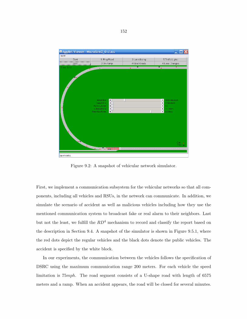
152

Figure 9.2: A snapshot of vehicular network simulator.

First, we implement a communication subsystem for the vehicular networks so that all com-

ponents, including all vehicles and RSUs, in the network can communicate. In addition, we

simulate the scenario of accident as well as malicious vehicles including how they use the

mentioned communication system to broadcast fake or real alarm to their neighbors. Last

but not the least, we fulfill the RD4 mechanism to record and classify the report based on

the description in Section 9.4. A snapshot of the simulator is shown in Figure 9.5.1, where

the red dots depict the regular vehicles and the black dots denote the public vehicles. The

accident is specified by the white block.

In our experiments, the communication between the vehicles follows the specification of

DSRC using the maximum communication range 200 meters. For each vehicle the speed

limitation is 75mph. The road segment consists of a U-shape road with length of 6575

meters and a ramp. When an accident appears, the road will be closed for several minutes.

153

 

Recall(Malicious)

99.98%

99.99%

100.00%

500vehicles/hour 800vehicles/hour 1000vehicles/hour 1200vehicles/hour

Figure 9.3: Recall of false accident reports.

The malicious vehicle will periodically broadcasts faked accident event if it doesn’t detect

a true event. Otherwise, it will keep silent.

9.5.2 Effectiveness of RD4

In this subsection, we show how effective the RD4 mechanism can detect the false accident

report inserted by malicious vehicles and confirm the true accident report generated by the

vehicles involved in the accident. This property is evaluated by the recall, which is defined

as the fraction in the amount of a certain event reported that our mechanism classifies

the report as this event. To be specific, in this application, the recall of false accident

report is defined as the fraction of the false accident reports that is detected by the RD4

mechanism, which is shown in Figure 9.5.2, while the recall of true accident report is defined

as the fraction of true accident reports confirmed by the RD4 mechanism, which is show

in Figure 9.5.2. In this experiment, we set the value of the maximum confidential score,

CSRself , CSRrsu, CSRpub and CSRreg to be 5, 3, 2, 1 respectively.

In the above two figures, the x-axis is the average vehicle density on the road and the

y-axis shows the recall. we can easily observe that the RD4 mechanism detects 100% false

accident reports in most cases and more than 95% nearby vehicles confirm a true accident

154

 

Recall(Accident)

94.00%

95.00%

96.00%

97.00%

98.00%

99.00%

100.00%

500vehicles/hour 800vehicles/hour 1000vehicles/hour 1200vehicles/hour

Figure 9.4: Recall of true accident reports.

report in all cases. These results validate that the proposed RD4 mechanism is very effective

in false accident report detection. We also find the the recall changes with the changing

of the vehicle density on the road. The recall of false accident report drops a little when

vehicle density grows, while the recall of true accident report increases with the increase

of vehicle density. This is because more traffic likely brings a lower average speed, which

is helpful to confirm a true accident in that vehicles are easier to get a low speed when an

accident happens, but a low speed is also helpful to confirm any accident report, so it will

affect the accuracy in detecting a false accident report contributes. Fortunately, based on

our experiment, we find that the effect is big only when the speed of vehicles is very low,

which depicts a heavy traffic jam and can be regards as a true accident. From this point of

view, when traffic is low, a false accident report is helping us to broadcast the true traffic

information.

9.5.3 Efficiency of RD4

After we validate the effective of RD4, we show the efficiency of RD4. Given that almost

all false accident reports will be detected and filtered, we only show how efficient RD4 can

155

 

Accident Report Confirmation Time

20.00%

40.00%

60.00%

80.00%

100.00%

0.5 min 1 min 1.5 min 2 min

500vehicle/hour 800vehicle/hour 1000vehicle/hour 1200vehicle/hour

Figure 9.5: Confirmation time of true accident reports.

 

Accident Report Propagation Range

70%

75%

80%

85%

90%

95%

100%

500 meter 1000 meter 1500 meter 2000 meter

500vehicle/hour 800vehicle/hour 1000vehicle/hour 1200vehicle/hour

Figure 9.6: Propagation range of true accident reports.

confirm true accident reports. Basically, we evaluate how fast a true accident report can be

confirmed and how far it can be propagated to be confirmed.

Figure 9.5.3 shows the percentage of nearby vehicles (within X meters) that a true acci-

dent report is confirmed. The x-axis depicts the time and the y-axis denotes the percentage

of confirmation. Four lines in different colors show different scenario of different average

vehicle density. We assume the total number of vehicles confirm the alarm in 2 minutes as

entity. In the figure, as the density increases from 500 to 800 vehicle per hour, more vehicles

detect the accident in the first half minutes due, which follows the same observation that

156

high average vehicle density helps to confirm accident reports. With the time passing, the

confirmation percentage increases almost linearly, approximately 25% every half minute,

which is because RD4 needs to collect sufficiency signal strength to confirm the accident re-

port. The confirmation rate increases quickly with the accumulation of the signal strength,

which may come from the fact of the slowing down vehicle velocity, the increasing average

density, and the more propagating accident reports when there is a true accident.

The propagation of a true accident confirmation is depicted in Figure 9.5.3, where the

x-axis records the distance from the vehicle to the accident location and the y-axis shows

the percentage of vehicles of the corresponding distance that confirm the accident report.

Similar to above experiment, four scenarios with different average vehicle densities are

reported in the figure. We can see that with the increasing of density, for the same range,

more percentage of vehicles detect the accident because high density will usually result in low

velocity and more confirmation messages about the accident report. Those several factors

interweave and produce this result. We can also see that more percentage of vehicles located

close to the accident confirm the true accident report than the vehicles located faraway from

the accident location. For example, when the density is more than 1000 vehicles per hour,

more than 97% vehicles within the range of 1000 meters confirm the accident report, and

the confirmation rate reduces to be between 85% and 90% when the vehicles are at the range

of 2000 meters. This shows the degrading of the signal strength of the accident with the

increasing of distance between the vehicles and the accident. Based on our simulation, even

though the distance goes to more than 2000 meters, a lot of vehicles can still confirm the

accident ahead on the road and they can take an early plan to switch the road. Furthermore,

if the average vehicle density is higher or the communication range is larger, the accident

confirmation can propagate to vehicles located further.

157

 

Message Complexity

1

1.01

1.02

1.03

1.04

1.05

500vehicles/hour 800vehicles/hour 1000vehicles/hour 1200vehicles/hour

Figure 9.7: Message complexity of RD4.

9.5.4 Message Complexity

Having seen the effectiveness and efficiency of the RD4 mechanism, we evaluate the overhead

of this mechanism. Figure 9.5.4 shows the number of messages delivered to confirm a true

accident report in terms of different average vehicle densities. In the figure, we observe that

the average number of messages send to ”persuade” a vehicle is very small, to be specific,

on average one message is enough. Actually, the cost only accumulates at the beginning of

an accident, with more vehicles broadcast alarm reports, this cost barely increases. Also, as

we expected, the message complexity decrease as the density grows. Because more vehicles

broadcast alarm reports once they detect the accident, it costs fewer messages on average

to convince a vehicle.

9.5.5 Effect of Maximum Confidential Scores

In the RD4 mechanism, different roles are assigned different capability in issuing a confi-

dential score. In this subsection, we try to tune the confidential score each role can issue

and compare the results which helps us to understand this mechanism. All experiments are

tested under traffic density of 1000 vehicles per hour.

158

Just as W_RSU, W_PUB influent the result less, because we assign public vehicle only 1 among 1000 vehicles.

W_PUB Recall(malicious) Recall(accident)

3 1 0.98881 2(original) 1 0.98836

0.5 1 0.987864 Table5: Tuning W_PUB CSRself 5 7 4 5 5 5 5 5 5 CSRrsu 3 3 3 4 2 3 3 3 3 CSRpub 2 2 2 2 2 3 0.5 2 1 CSRreg 1 1 1 1 1 1 1 2 0.5 Recall(false) 1 0.996 1 1 1 1 1 0.923 1 Recall(true) 0.988 0.990 0.988 0.989 0.988 0.989 0.998 0.994 0.968

Figure 9.8: Effect of maximum confidential scores.

Figure 9.5.5 shows the effect of tuning CSRs to the recalls. Each data column in the

figure reports a set of the maximum CSRs of four roles and the resulted recalls using this

set of CSRs. The first data column is the set of the maximum CSRs used in experiments in

above several subsections. From the figure, we can see that tuning the CSRrsu and CSRpub

will not change the recall too much. This is because in our simulation the number of RSUs

and public vehicles are very small, which is close to the reality, but we still see a slight

improvement in the recall of true accident report when CSRrsu and CSRpub are assigned

higher value, which reflects the fact that those roles are worthy to be trusted. Tuning the

value of CSRself affects both recalls. If we increase the value of CSRself , the vehicles

become more sensitive, thus they will confirm more true accident reports as well as more

false accident reports. Thus, to detect and filter the false accident report, we should not

make the vehicles too sensitive in confirming events.

Compared with above three CSRs, tuning CSRreg affects the recalls most. When we

increase the value of CSRreg, the recall of false accident reports degrades a lot but the

recall of true accident reports increases, because of the large amount of regular vehicles in

the system and higher probability of regular vehicles to be malicious vehicles than other

types of components in the system. Similarly, when we decrease the value of CSRreg, less

true accident reports are confirmed, but more false accident reports are confirmed. Thus,

we need to find a good value for CSRreg to balance the recall of false accident reports and

the recall of true accident reports.

159

In summery, we find that the RD4 mechanism works effectively and efficiently in de-

tecting and filtering false accident reports as well as confirming true accident reports at a

low cost. A tradeoff should be made to assign picking maximum confidential score for each

role.

160

CHAPTER 10

CONCLUSIONS AND FUTURE WORK

10.1 Conclusion

In this dissertation, we we envision that the success of the sensing system applications are

largely depending on whether we can collect high quality data using the deployed sensing

systems. Thus, we propose to integrate data quality management in any energy efficient

sensing system design. As a result, a general framework named Orchis has been proposed to

manage data quality in sensing systems. In the framework, we first analyze the characteris-

tics of the sensing data. Then, we propose a set of data consistency models that are the core

of our framework and are used to evaluate the quality of the collected data. Moreover, we

devise a set of protocols to achieve the goals of both saving energy and collecting high qual-

ity data. For example, an energy efficient adaptive lady protocol is designed to collect high

quality data in an energy efficient way. To improve the data quality of the collected data,

we also propose a systematic mechanism to detect and filter the deceptive data. Finally, we

argue that the protocol in sensing systems should be energy efficient, so we formally define

a set of models, lifetime models for sensor networks, to evaluate the energy efficient of the

proposed protocol. According to the results from both the simulation based on more than

100 sensors using TOSSIM and the prototype implementation based on 13 Mica2 Motes,

we validate the effectiveness of our proposed protocol.

10.2 Future Work

After having introduced the work we have done in this dissertation, we are in a position to

depict what we plan to do in future research.

161

10.2.1 Complete and Extend the Orchis Framework

We plan to completing some undeveloped protocols in the design of the framework, such

as several other mechanisms to detect and filter deceptive data and traffic-differentiated

cross-layer protocol. Then we will extend the Orchis framework to fit Cyber-Physical Sys-

tems, for example, consistency models can take advantage of the features of the physical

properties. In other words, to including some physical laws into the consistency models

will be very helpful in consistency checking as well as deceptive data detection. Moreover,

the system protocols will also be adjusted to fit the characteristics of cyber-physical sys-

tems accordingly. Mechanisms that are used to replace the detected deceptive data and

missing data will be explored. In the case when we cannot avoid dropping some sensing

data due to the constrained computation, communication and storage, we will drop less

important data based on the physical characteristics of the data. Furthermore, cross-layer

traffic-differentiated data collection protocols will be designed to transmit data in physical

priority ways. Finally, we will implement and evaluate more protocols we mention in the

deceptive data detection and filtering framework.

10.2.2 Privacy and Security in Sensing Systems

In addition, Security and privacy are always of importance for modern systems. In cyber-

physical systems or extended sensing systems, the deep distributed physical environment

both increases the risk and offers new opportunities. For example, sensitive biomedical data

collected from body area networks may release critical personal information. A security

breach may result in fatal physical damage, such as vehicle crash. Thus, it is a big challenge

to preserve privacy and security in such an open environment; whereas, the distinct physical

features can be also utilized to authenticate legislate users and detect malicious attackers. In

this direction, I plan to extend the concept of adaptive privacy and propose novel protocols

to preserve privacy and improve security.

162

10.2.3 Sensing System Applications in Healthcare Systems

Finally, Cyber-physical systems and the extended sysnsing systems can be used in a great

deal of applications. One of the most promising applications is in developing modern health-

self-care systems. We proposed a Smart Phone Assisted Chronic Illness Self-Management

System in [Sha et al., 2008c], which uses participatory sensing to investigate the causes of

chronic illness and discover potential approaches to prevent chronic illness. In this system,

all above proposed techniques will be integrated in a prototype system and they will be

evaluated in real deployment.

163

REFERENCES

[Adam et al., 2004] Adam, N., Janeja, V. P., and Atluri, V. (2004). Neighborhood based

detection of anomalies in high dimensional spatio-temporal sensor datasets. In Proceedings

of the 2004 ACM symposium on Applied computing.

[Akkaya and Younis, 2003] Akkaya, K. and Younis, M. (2003). An energy-aware qos routing

protocol for wireless sensor networks. In Proceedings of the IEEE Workshop on Mobile

and Wireless Networks (MWN’03).

[Akyildiz et al., 2002] Akyildiz, I. F., Su, W., Sankarasubramaniam, Y., and Cayirci, E.

(2002). A survey on sensor networks. IEEE Communications Magazine, 40(8):102–114.

[Arisha et al., 2002] Arisha, K., Youssef, M., and Younis, M. (2002). Energy-aware tdma-

based mac for sensor networks. In IEEE IMPACCT 2002.

[Arora et al., 2005] Arora, A. et al. (2005). Exscal: Elements of an extreme scale wireless

sensor network. In Proceedings of the 11th IEEE International Conference on Embedded

and Real-Time Computing Systems and Applications (RTCSA 2005).

[Atkins, 2006] Atkins, E. M. (2006). Cyber-physical aerospace: Challenges and future di-

rections in transportation and exploration systems. In NSF Workshop on Cyber-Physical

Systems.

[Bao and J.J.Garcia-Luna-Aceves, 2001] Bao, L. and J.J.Garcia-Luna-Aceves (2001).

Channel access scheduling in ad hoc networks with unidirectional links. In International

Workshop on Discrete Algorithms and Methods for Mobile Computing and Communica-

tions (DIALM’01).

164

[Batalin et al., 2004] Batalin, M. et al. (2004). Call and responses: Experiments in sampling

the environment. In Proc. of ACM SenSys 2004.

[Bhardwaj and Chandrakasan, 2002] Bhardwaj, M. and Chandrakasan, A. (2002). Bound-

ing the lifetime of sensor networks via optimal role assignments. In Proceedings of IEEE

INFOCOM 2002.

[Bhardwaj et al., 2001] Bhardwaj, M., Garnett, T., and Chandrakasan, A. P. (2001). Upper

bounds on the lifetime of sensor networks. In Proceedings of ICC 2001.

[Bharghavan et al., 1994] Bharghavan, V., Demers, A., Shenker, S., and Zhang, L. (1994).

Macaw: A media access protocol for wireless lans. In Proc. of ACM SIGCOMM’94.

[Bishop, 2000] Bishop, R. (2000). A survey of intelligent vehicle applications worldwide. In

Proc. of IEEE intelligent Vehicles Symposium 2000.

[Blough and Santi, 2002] Blough, D. M. and Santi, P. (2002). Investigating upper bounds

on network lifetime extension for cell-based energy conservation techniques in stationary

ad hoc networks. In Proceedings of the 8th Annual ACM/IEEE International Conference

on Mobile Computing and Networking(MobiCom’02).

[Bokareva et al., 2006] Bokareva, T. et al. (2006). Wireless sensor networks for battlefield

surveillance. In Proceedings of Land Warfare Conference 2006.

[Braginsky and Estrin, 2002] Braginsky, D. and Estrin, D. (2002). Rumor routing algorithm

for sensor networks. In Proceedings of the First Workshop on Sensor Networks and

Applications(WSNA’02).

[Campbell et al., 2006] Campbell, A. et al. (2006). People-centric urban sensing. In Pro-

ceedings of the 2nd Annual International Workshop on Wireless Internet.

165

[Cerpa and Estrin, 2002] Cerpa, A. and Estrin, D. (2002). ASCENT: Adaptive self-

configuring sensor network topologies. In Proc. of IEEE Conference on Computer Com-

munications (INFOCOM’02).

[Chang and Tassiulas, 2000] Chang, J. H. and Tassiulas, L. (2000). Maximum lifetime rout-

ing in wireless sensor networks. In Proceedings of Advanced Telecommunications and

Information Distribution Research Program(ARIRP’00).

[Chen et al., 2001] Chen, B., Jamieson, K., Balakrishnan, H., and Morris, R. (2001). SPAN:

An energy-efficient coordination algorithm for topology maintenance in ad-hoc wireless

networks. In Proceedings of the 7th Annual ACM/IEEE International Conference on

Mobile Computing and Networking(MobiCom’01).

[Chipara et al., 2005] Chipara, O., Lu, C., and Roman, G. (2005). Efficient power manage-

ment based on application timing semantics for wireless sensor networks. In Proceedings

of the 25th International Conference on Distributed Computing Systems (ICDCS’05).

[COMPASS, ] COMPASS. Compass: Collaborative multiscale processing and architecture

for sensornetworks.

[crossbow, ] crossbow. Crossbow technology inc.

[Dai and Han, 2003] Dai, H. and Han, R. (2003). A node-centric load balancing algorithm

for wireless sensor networks. In Proceedings of IEEE GLOBECOM’03.

[Dam and Langendoen, 2003] Dam, T. and Langendoen, K. (2003). An adaptive energy-

efficient mac protocol for wireless sensor networks. In Proc. of ACM SenSys 2003.

[Dasgupta et al., 2003] Dasgupta, K. et al. (2003). An efficient clustering-based heuristic for

data gathering and aggregation in sensor networks. In Proceedings of the IEEE Wireless

Communications and Networking Conference (WCNC’03).

166

[Datta, 2003] Datta, A. (2003). Fault-tolerant and energy-efficient permutation routing

protocol for wireless networks. In International Parallel and Distributed Processing Sym-

posium (IPDPS’03).

[Deb et al., 2002] Deb, B., Bhatnagar, S., and Nath, B. (2002). A topology discovery algo-

rithm for sensor networks with applications to network management. In In IEEE CAS

workshop(short paper).

[Deb et al., 2003] Deb, B., Bhatnagar, S., and Nath, B. (2003). Information assurance in

sensor networks. In Proceedings of 2nd ACM International Workshop on Wireless Sensor

Networks and Applications.

[Ding et al., 2003] Ding, M., Cheng, X., and Xue, G. (2003). Aggregation tree construction

in sensor networks. In Proceedings of the 58th IEEE Vehicular Technology Conference’03.

[Douglas et al., 2006] Douglas, C. et al. (2006). Cyber-physical systems and wildland fire

or contaminant identification and tracking dynamic data-driven application systems. In

NSF Workshop on Cyber-Physical Systems.

[DSRC, ] DSRC. Dedicated short range communications (dsrc) home.

[Du et al., 2005] Du, J., Shi, W., and Sha, K. (2005). Asymmetry-aware link quality services

in wireless sensor networks. In Proceedings of the 2005 IFIP International Conference on

Embedded and Ubiquitous Computing.

[Duarte-Melo and Liu, 2003] Duarte-Melo, E. and Liu, M. (2003). Analysis of energy con-

sumption and lifetime of heterogeneous wireless sensor networks. In in Proc. IEEE Globe-

com.

167

[Elnahrawy and Nath, 2003] Elnahrawy, E. and Nath, B. (2003). Cleaning and querying

noisy sensors. In Proceedings of the Second ACM Workshop on Wireless Sensor Networks

and Applications (WSNA).

[Elson et al., 2002] Elson, J., Girod, L., and Estrin, D. (2002). Fine-grained network time

synchronization using reference broadcasts. In Proc. of the Fifth Symposium on Operating

Systems Design and Implementation(OSDI).

[Estrin et al., 2002] Estrin, D., Culler, D., Pister, K., and Sukhatme, G. (2002). Connecting

the physical world with pervasive networks. IEEE Pervasive Computing, 1(1):59–69.

[Estrin et al., 1999] Estrin, D. et al. (1999). Next century challenges: Scalable coordination

in sensor networks. In Proceedings of the 5th Annual ACM/IEEE International Confer-

ence on Mobile Computing and Networking (MobiCom’99).

[Estrin et al., 2003] Estrin, D., Michener, W., and Bonito, G. (2003). Environmental cyber-

infrastructure needs for distributed sensor networks. A Report From a National Science

Foundation Sponsored Worksop.

[Faruque and Helmy, 2004] Faruque, J. and Helmy, A. (2004). RUGGED: Routing on fin-

gerprint gradients in sensor networks. In Proceedings of IEEE Int’l Conf. on Pervasive

Services.

[Ganesan et al., 2002] Ganesan, D. et al. (2002). Highly resilient, energy efficient multi-

path routing in wireless sensor networks. Mobile Computing and Communications Re-

view(MC2R), 1(2).

[Garces and Garcia-Luna-Aceves, 1997a] Garces, R. and Garcia-Luna-Aceves, J. J. (1997a).

Collision avoidance and resolution multiple access: First-success protocols. In Proceedings

of IEEE International Conference on Communications (ICC’97).

168

[Garces and Garcia-Luna-Aceves, 1997b] Garces, R. and Garcia-Luna-Aceves, J. J.

(1997b). Collision avoidance and resolution multiple access with transmission groups.

In Proc. of IEEE Conference on Computer Communications (INFOCOM’97).

[Garrett et al., 2006] Garrett, J., Moura, J., and Sanfilippo, M. (2006). Sensor-data driven

proactive management of infrastructure systems. In NSF Workshop on Cyber-Physical

Systems.

[Gedik and Liu, 2005] Gedik, B. and Liu, L. (2005). Location privacy in mobile systems:

A personalized anonymization model. In Proc. of the 25th International Conference on

Distributed Computing Systems.

[Gnawali et al., 2006] Gnawali, O. et al. (2006). The tenet architecture for tiered sensor

networks. In Proc. of ACM SenSys 2006.

[Goel and Estrin, 2003] Goel, A. and Estrin, D. (2003). Simultaneous optimization for

concave costs: Single sink aggregation or single source buy-at-bulk. In Proceedings of the

14th Annual ACM-SIAM Symposium on Discrete Algorithms’03.

[Goodman et al., 1989] Goodman, D., Valenzuela, R., Gayliard, K., and Ramamurthy, B.

(1989). Packet reservation multiple access for local wireless communications. IEEE

Transactions on Communications, 37(8):885–890.

[Gupta and Younis, 2003] Gupta, G. and Younis, M. (2003). Fault-tolerant clustering of

wireless sensor networks. In in the Proceedings of the IEEE Wireless Communication and

Networks Conference (WCNC 2003).

[Gupta et al., 2008] Gupta, H. et al. (2008). Efficient gathering of correlated data in sensor

networks. ACM Transactions on Sensor Networks, 4(1).

169

[Gupta et al., 2005] Gupta, R., Puri, A., and Ramamritham, K. (2005). Executing inco-

herency bounded continuous queries at web data aggregators. In Proc. of 14th Interna-

tional World Wide Web Conference.

[Haeberlen et al., 2004] Haeberlen, A. et al. (2004). Practical robust localization over large-

scale 802.11 wireless networks. In Proceedings of the 10th Annual ACM/IEEE Interna-

tional Conference on Mobile Computing and Networking(MobiCom’04).

[Hamdaoui and Ramanathan, 2006] Hamdaoui, B. and Ramanathan, P. (2006). Energy-

Efficient and MAC-Aware Routing for Data Aggregation in Sensor Networks. IEEE Press.

[He et al., 2002] He, T., Blum, B., Stankovic, J. A., and Abdelzaher, T. F. (2002). Aida:

Adaptive application independent data aggregation in wireless sensor networks. ACM

Transactions on Embeded Computing Systems, 40(8):102–114.

[He et al., 2003] He, T., Stankovic, J. A., Lu, C., and Abdelzaher, T. (2003). Speed: A

stateless protocol for real-time communication in sensor networks. In Proceedings of

IEEE ICDCS’03.

[Heinzelman et al., 2002] Heinzelman, W., Chandrakasan, A., and Balakrishnan, H. (2002).

An application-specific protocol architecture for wireless microsensor networks. IEEE

Transactions on Wireless Communications, 1(4):660–670.

[Heinzelman et al., 1999] Heinzelman, W., Kulik, J., and Balakrishnan, H. (1999). Adap-

tive protocols for information dissemination in wireless sensor networks. In Proceedings

of the 5th Annual ACM/IEEE International Conference on Mobile Computing and Net-

working(MobiCom’99), pages 174–185.

[Heinzelman et al., 2000] Heinzelman, W. R., Chandrakasan, A., and Balakrishnan, H.

(2000). Energy-efficient communication protocol for wireless micorsensor networks. In

Proceedings of HICSS’00.

170

[Hill et al., 2000] Hill, J., Szewczyk, R., Woo, A., Hollar, S., Culler, D., and Pister, K.

(2000). System architecture directions for networked sensors. In Proceedings the 9th

ASPLOS’00, pages 93–104.

[Hodge and Austin, 2004] Hodge, V. and Austin, J. (2004). A survey of outlier detection

methodologies. Artificial Intelligence Review, 22:85–126.

[IEEE802.11, 1999] IEEE802.11 (1999). Part 11: Wireless lan medium access control (mac)

and physical layer (phy) specification.

[IEEE802.15.4/D18, 2003] IEEE802.15.4/D18 (2003). Draft standard: Low rate wireless

personal area networks.

[Intanagonwiwat et al., 2002] Intanagonwiwat, C., Estrin, D., Govindan, R., and Heide-

mann, J. (2002). Impact of network density on data aggregation in wireless sensor net-

works. In Proceedings of IEEE ICDCS’02.

[Intanagonwiwat et al., 2000] Intanagonwiwat, C., Govindan, R., and Estrin, D. (2000). Di-

rected diffusion: A scalable and robust communication paradigm for sensor networks. In

Proceedings of the 6th Annual ACM/IEEE International Conference on Mobile Comput-

ing and Networking(MobiCom’00).

[ITSA and DoT, 2002] ITSA and DoT (2002). National intelligent transportation systems

program plan: A ten-year vision. A Report from Intelligent Transportation Society of

America and Departemnt of Transportation.

[Jain and Chang, 2004] Jain, A. and Chang, E. (2004). Adaptive sampling for sensor net-

works. In Proc. of the 1st international workshop on Data management for sensor net-

works: in conjunction with VLDB 2004.

171

[Janakiram et al., 2006] Janakiram, D., Reddy, A., and Kumar, A. (2006). Outlier detection

in wireless sensor networks using bayesian belief networks. In Proceeedings of the 1st

International Conference on Communication System Software and Middleware.

[Jeffery et al., 2006] Jeffery, S. et al. (2006). Declarative support for sensor data cleaning.

In Proceeedings of The 4th International Conference on Pervasive Computing.

[Kalpakis et al., 2002] Kalpakis, K., Dasgupta, K., and Namjoshi, P. (2002). Maximum

lifetime data gathering and aggregation in wireless sensor networks. In Proceedings of

IEEE Networks’02 Conference(NETWORKS02).

[Kang and Poovendran, 2003] Kang, I. and Poovendran, R. (2003). Maximizing static net-

work lifetime of wireless broadcast adhoc networks. In IEEE 2003 International Confer-

ence on Communications.

[Karp and Kung, 2000] Karp, B. and Kung, H. T. (2000). Gpsr: greedy perimeter stateless

routing for wireless networks. In Proceedings of the 6th Annual ACM/IEEE International

Conference on Mobile Computing and Networking(MobiCom’00).

[Khanna et al., 2004] Khanna, G., Bagchi, S., and Wu, Y. (2004). Fault tolerant energy

aware data dissemination protocol in sensor networks. In 2004 International Conference

on Dependable Systems and Networks (DSN’04).

[Krause et al., 2008] Krause, A. et al. (2008). Toward community sensing. In Proc.

of the fourth International Conference on Information Processing in Sensor Networks

(IPSN’08).

[Larkey et al., 2006] Larkey, L., Bettencourt, L., and Hagberg, A. (2006). In-situ data

quality assurance for environmental applications of wireless sensor networks. Technical

Report Report LA-UR-06-1117, Los Alamos National Laboratory.

172

[Lazaridis et al., 2004] Lazaridis, I. et al. (2004). Quasar: quality aware sensing architec-

ture. ACM SIGMOD Record, Special section on sensor network technology and sensor

data management, 2:26–31.

[Lazaridis and Mehrotra, 2003] Lazaridis, I. and Mehrotra, S. (2003). Capturing sensor-

generated time series with quality guarantees. In Proceedings of 19th International Con-

ference on Data Engineering.

[Levis et al., 2003] Levis, P., Lee, N., Welsh, M., and Culler, D. (2003). Tossim: Accurate

and scalable simulation of entire tinyos applications. In Proc. of ACM SenSys 2003.

[Li et al., 2007] Li, H. et al. (2007). The development of a wireless sensor network sens-

ing node utilising adaptive self-diagnostics. In Proceeedings of the Second International

Workshop on Self-Organizing Systems.

[Li et al., 2006] Li, M., Ganesan, D., and Shenoy, P. (2006). PRESTO: Feedback-driven

data management in sensor networks. In Proc. of the NSDI’06.

[Lin and Gerla, 1997] Lin, C. and Gerla, M. (1997). Adaptive clustering for mobile wireless

networks. IEEE Journal of Selected areas in Communications, 15(7).

[Lindsey et al., 2002] Lindsey, S., Raghavendra, C., and Sivalingam, K. M. (2002). Data

gathering algorithms in sensor networks using energy metrics. IEEE Transactions on

Parallel and Distributed Systems, 13(8):924–936.

[Lindsey et al., 2001] Lindsey, S., Raghavendra, C. S., and Sivallingam, K. (2001). Data

gathering in sensor networks using the energy*delay metric. In Proceedings of the IPDPS

Workshop on Issues in Wireless Networks and Mobile Computing.

173

[Lu et al., 2005] Lu, C. et al. (2005). A spatiotemporal query service for mobile users

in sensor networks. In Proceedings of the 25th International Conference on Distributed

Computing Systems (ICDCS’05).

[Luo et al., 2005] Luo, H., Luo, J., and Liu, Y. (2005). Energy efficient routing with adap-

tive data fusion in sensor networks. In Proceedings of the Third ACM/SIGMOBILEe

Workshop on Foundations of Mobile Computing’05.

[Madden et al., 2005] Madden, S. et al. (2005). Tinydb: An acqusitional query processing

system for sensor networks. ACM Transactions on Database Systems, 30(1).

[Madden et al., 2002] Madden, S., Franklin, M. J., Hellerstein, J., and Hong, W. (2002).

Tag: A tiny aggregation service for ad-hoc sensor network. In Proc. of the Fifth USENIX

Symposium on Operating Systems Design and Implementation.

[Mainland et al., 2005] Mainland, G., Parkes, D., and Welsh, M. (2005). Decentralized,

adaptive resource allocation for sensor networks. In Proc. of the NSDI’05.

[Manjeshwar and Agrawal, 2001] Manjeshwar, A. and Agrawal, D. P. (2001). TEEN: A

protocol for enhanced efficiency in wireless sensor networks. In Proceedings of the first

International Workshop on Parallel and Distributed Computing Issues in Wireless Net-

works and Mobile Computing.

[Manjeshwar and Agrawal, 2002] Manjeshwar, A. and Agrawal, D. P. (2002). Apteen: A

hybrid protocol for efficient routing and comprehensive information retrieval in wireless

sensor networks. In Proceedings of the 2nd International Workshop on Parallel and Dis-

tributed Computing Issues in Wireless Networks and Mobile Computing.

[Marbini and Sacks, 2003] Marbini, A. and Sacks, L. (2003). Adaptive sampling mecha-

nisms in sensor networks. In London Communications Symposium.

174

[Martinez et al., 2004] Martinez, K., Hart, J. K., and r. Ong (2004). Environmental sensor

networks. IEEE Computer Magazine, 37(8):50–56.

[Mhatre et al., 2004] Mhatre, V. et al. (2004). A minimum cost heterogeneous sensor net-

work with a lifetime constraint. IEEE Transaction on Mobile Computing.

[Min and Chandrakasan, 2003] Min, R. and Chandrakasan, A. (2003). Mobicom poster: top

five myths about the energy consumption of wireless communication. Mobile Computing

and Communications Review, 7(1):65–67.

[Moore et al., 2004] Moore, D., Leonard, J., Rus, D., and Teller, S. (2004). Robust dis-

tributed network localization with noisy range measurements. In Proc. of ACM SenSys

2004.

[Muir and Garcia-Luna-Aceves, 1998] Muir, A. and Garcia-Luna-Aceves, J. J. (1998). An

efficient packet sensing mac protocol for wireless networks. Mobile Networks and Appli-

cations, 3(2):221–234.

[Mukhopadhyay et al., 2004a] Mukhopadhyay, S., Panigrahi, D., and Dey, S. (2004a). Data

aware, low cost error correction for wireless sensor networks. In Proceeedings of 2004

IEEE Wireless Communications and Networking Conferenc.

[Mukhopadhyay et al., 2004b] Mukhopadhyay, S., Panigrahi, D., and Dey, S. (2004b).

Model based error correction for wireless sensor networks. In Proceeedings of the 1st

Annual IEEE Communications Society Conference on Sensor and Ad Hoc Communica-

tions and Networks.

[Nath et al., 2007] Nath, S., Liu, J., and Zhao, F. (2007). Sensormap for wide-area sensor

webs. Computer, 40(7):106–109.

175

[Peterson and Davie, 2003] Peterson, L. L. and Davie, B. (2003). Computer Networks: A

Systems Approach. Morgan Kaufmann.

[Picconi et al., 2006] Picconi, F. et al. (2006). Probabilistic validation of aggregrated data

for v2v traffic information systems. In Proc. of the Third ACM International Workshop

on Vehicular Ad Hoc Networks (VANET 2006).

[Polastre et al., 2004] Polastre, J., Hill, J., and Culler, D. (2004). Veratile low power media

access for wireless sensor networks. In Proc. of ACM SenSys 2004.

[Polastre et al., 2005] Polastre, J., Szewczyk, R., and Culler, D. (2005). Telos: Enabling

ultra-low power wireless research. In Proc. of the 14th International Conference on In-

formation Processing in Sensor Networks: Special track on Platform Tools and Design

Methods for Network Embedded Sensors (IPSN/SPOTS).

[Pottie and Kaiser, 2000] Pottie, G. and Kaiser, W. (2000). Wireless integrated network

sensors. Communications of the ACM, 43(5):51–58.

[Rajendran et al., 2003] Rajendran, V., Obraczka, K., and Garcia-Luna-Aceves, J. J.

(2003). Energy-efficient, collision-free medium access control for wireless sensor networks.

In Proc. of ACM SenSys 2003.

[Ramakrishnan, 1998] Ramakrishnan, R. (1998). Database Management Systems.

WCB/McGraw-Hill.

[Sadagopan et al., 2003] Sadagopan, N. et al. (2003). The acquire mechanism for efficient

querying in sensor networks. In Proceedings of the First International Workshop on

Sensor Network Protocol and Applications.

176

[Sadagopan and Krishnamachari, 2004] Sadagopan, N. and Krishnamachari, B. (2004).

Maximizing data extraction in energy-limited sensor networks. In Proceedings of IEEE

INFOCOM 2004.

[Sadler et al., 2004] Sadler, C., Zhang, P., Martonosi, M., and Lyon, S. (2004). Hardware

design experiences in zebranet. In Proc. of ACM SenSys 2004.

[Santi and Chessa, 2002] Santi, P. and Chessa, S. (2002). Crash faults identification in

wireless sensor networks. COMPUTER COMMUNICATIONS, 25(14):1273–1282.

[Schurgers and Srivastava, 2001] Schurgers, C. and Srivastava, M. (2001). Energy efficient

routing in wireless sensor networks. In MILCOM Proceedings on Communications for

Network-Centric Operations: Creating the Information Force.

[Seada et al., 2004] Seada, K., Zuniga, M., Helmy, A., and Krishnamachari, B. (2004).

Energy-efficient forwarding strategies for geographic routing in lossy wireless sensor net-

works. In Proc. of ACM SenSys 2004.

[SenseWeb, ] SenseWeb. Microsoft research.

[Sha et al., 2006a] Sha, K., Du, J., and Shi, W. (2006a). Wear: A balanced, fault-tolerant,

energy-efficient routing protocol for wireless sensor networks. International Journal of

Sensor Networks, 1(2).

[Sha et al., 2008a] Sha, K. et al. (2008a). Data quality and failures characterization of

sensing data in environmental applications. In Proceedings of CollaborateCom 2008.

[Sha et al., 2008b] Sha, K. et al. (2008b). Modeling data consistency in wireless sensor

networks. In Workshop Proceedings of ICDCS 2007 (WWASN 2007.

177

[Sha et al., 2008c] Sha, K. et al. (2008c). Spa: Smart phone assisted chronic illness self-

management with participatory sensing. In Proceedings of The 2nd International Work-

shop on Systems and Networking Support for Healthcare and Assisted Living Environ-

ments (Healthnet’08), in conjunction with MobiSys08.

[Sha and Shi, 2004] Sha, K. and Shi, W. (2004). Revisiting the lifetime of wireless sensor

networks. In Proceedings of ACM SenSys’04.

[Sha and Shi, 2005] Sha, K. and Shi, W. (2005). Modeling the lifetime of wireless sensor

networks. Sensor Letters, 3(2):126–135.

[Sha and Shi, 2006a] Sha, K. and Shi, W. (2006a). On the effects of consistency in data

operations in wireless sensor networks. In Proceedings of IEEE 12th International Con-

ference on Parallel and Distributed Systems.

[Sha and Shi, 2006b] Sha, K. and Shi, W. (2006b). Using wireless sensor networks for fire

rescue applications: Requirements and challenges. In Proceedings of IEEE EIT 2006.

[Sha and Shi, 2008] Sha, K. and Shi, W. (2008). Consistency-driven data quality man-

agement in wireless sensor networks. Journal of Parallel and Distributed Computing,

68(9):1207–1221.

[Sha et al., 2006b] Sha, K., Shi, W., and Sellamuthu, S. (2006b). Load Balanced Query

Protocols for Wireless Sensor Networks. Wiley-IEEE Press.

[Sha et al., 2004] Sha, K., Zhu, Z., and Shi, W. (2004). Capricorn: A large scale wireless

sensor network simulator. Technical Report MIST-TR-2004-001, Wayne State University.

[Shah and Rabaey, 2002] Shah, R. and Rabaey, J. (2002). Energy aware routing for low

energy ad hoc sensor networks. In Proceedings of the IEEE Wireless Communications

and Networking Conference (WCNC’02).

178

[Shah et al., 2003] Shah, S., Dharmarajan, S., and Ramamritham, K. (2003). An efficient

and resilient approach to filtering and disseminating streaming data. In Proc. of 29th

International Conference on Very Large Data Bases.

[Sharaf et al., 2004] Sharaf, M., Beaver, J., Labrinidis, A., and Chrysanthis:, P. (2004).

Balancing energy efficiency and quality of aggregate data in sensor networks. The VLDB

Journal, 13(4):384–403.

[Shekhar et al., 2003] Shekhar, S., Lu, C., and Zhang, P. (2003). A unified approach to

spatial outliers detection. Geoinformatica, 7(2).

[Shih et al., 2001] Shih, E. et al. (2001). Physical layer driven protocol and algorithm design

for energy-efficient wireless sensor networks. In Proceedings of the 7th Annual ACM/IEEE

International Conference on Mobile Computing and Networking (MobiCom’01), Rome,

Italy.

[Shnayder et al., 2004] Shnayder, V. et al. (2004). Simulating the power consumption of

large-scale sensor network applications. In Proc. of ACM SenSys 2004.

[Shrivastava et al., 2004] Shrivastava, N., Buragohain, C., Suri, S., and Agrawal, D. (2004).

Medians and beyond: New aggregation techniques for sensor networks. In Proc. of ACM

SenSys 2004.

[Shrivastava et al., 2006] Shrivastava, N. et al. (2006). Target tracking with binary proxim-

ity sensors: Fundamental limits, minimal descriptions, and algorithms. In Proc. of ACM

SenSys 2006.

[Simon et al., 2004] Simon, G., Ledeczi, A., and Maroti, M. (2004). Sensor network-based

countersniper system. In Proc. of ACM SenSys 2004.

179

[Skordylis et al., 2006] Skordylis, A., Guitton, A., and Trigoni, N. (2006). Correlation-based

data dissemination in traffic monitoring sensor networks. In Proceedings of the 2006 ACM

CoNEXT conference.

[SNA, ] SNA. A network architecture for wireless sensor networks.

[Srivastava et al., 2006] Srivastava, M. et al. (2006). Wireless urban sensing systems. Tech-

nical Report CENS Technical Report No. 65, CENS.

[Ssu et al., 2006] Ssu, K. et al. (2006). Detection and diagnosis of data inconsistency failures

in wireless sensor networks. Computer Networks: The International Journal of Computer

and Telecommunications Networking, 50(9).

[Sutton and Barto, 1998] Sutton, R. and Barto, A. (1998). Review of Reinforcement Learn-

ing: An Introduction. The MIT Press.

[Szewczyk et al., 2004a] Szewczyk, R. et al. (2004a). Habitat monitoring with sensor net-

works. Communications of the ACM, 47(6):34–40.

[Szewczyk et al., 2004b] Szewczyk, R., Mainwaring, A., Polastre, J., and Culler, D. (2004b).

An analysis of a large scale habitat monitoring application. In Proc. of ACM SenSys 2004.

[Tanenbaum and van Steen, 2002] Tanenbaum, A. S. and van Steen, M. (2002). Distributed

Systems: Principles and Paradigms. Prentice-Hall.

[Tang and Xu, 2006] Tang, X. and Xu, J. (2006). Extending network lifetime for precision-

constrained data aggregation in wireless sensor networks. In Proc. of IEEE Conference

on Computer Communications (INFOCOM’06).

180

[Tatbul et al., 2004] Tatbul, N. et al. (2004). Confidence-based data management for per-

sonal area sensor networks. In Proceeedings of the 1st international workshop on Data

management for sensor networks: in conjunction with VLDB 2004.

[Thiemann et al., 2008] Thiemann, C., Treiber, M., and Kesting, A. (2008). Estimating ac-

celeration and lane-changing dynamics based on ngsim trajectory data. In Transportation

Research Board Annual Meeting.

[Traffic Simulator, ] Traffic Simulator. Traffic simulator.

[Trappe et al., 2005] Trappe, W., Zhang, Y., and Nath, B. (2005). Miami: methods and

infrastructure for the assurance of measurement information. In Proceedings of the 2nd

international workshop on Data management for sensor networks.

[VII, ] VII. Vehicle infrastructure integration.

[Wavescope, ] Wavescope. Wavescope: An adaptive wireless sensor network system for high

data-rate applications.

[Welsh and Mainland, 2004] Welsh, M. and Mainland, G. (2004). Programming sensor net-

work using abstract regions. In Proceedings of the First USENIX/ACM Networked System

Design and Implementation.

[Woo and Culler, 2001] Woo, A. and Culler, D. (2001). A transmission control scheme for

media access in sensor networks. In Proceedings of the 7th Annual ACM/IEEE Interna-

tional Conference on Mobile Computing and Networking (MobiCom’01), Rome, Italy.

[Xu et al., 2004] Xu, N. et al. (2004). A wireless sensor network for structural monitoring.

In Proc. of ACM SenSys 2004.

181

[Xu et al., 2001a] Xu, Y., Heidemann, J., and Estrin, D. (2001a). Geography-informed

energy conservation for ad hoc routing. In Proceedings of the 7th Annual ACM/IEEE

International Conference on Mobile Computing and Networking(MobiCom’01).

[Xu et al., 2001b] Xu, Y., Heidemann, J., and Estrin, D. (2001b). Geography-informed

energy conservation for ad-hoc routing. In Proceedings of the 7th Annual ACM/IEEE

International Conference on Mobile Computing and Networking(MobiCom’01).

[Xue and Ganz, 2004] Xue, Q. and Ganz, A. (2004). On the lifetime of large scale sensor

networks. Elsevier Computer Communications.

[Yao and Gehrke, 2002] Yao, Y. and Gehrke, J. (2002). The cougar approach to in-network

query processing in sensor networks. ACM SIGMOD Record, 31(3):9–18.

[Ye et al., 2004] Ye, F. et al. (2004). Statistical en-route filtering of injected false data in

sensor networks. In Proceeedings of IEEE Infocom 2004.

[Ye et al., 2005] Ye, F. et al. (2005). Statistical en-route filtering of injected false data in

sensor networks. IEEE Journal on Selected Areas in Communications, 23:839–850.

[Ye et al., 2002] Ye, W., Heidemann, J., and Estrin, D. (2002). An energy-efficient mac

protocol for wireless sensor networks. In Proc. of IEEE Conference on Computer Com-

munications (INFOCOM’02), New York, NY.

[Younis et al., 2002] Younis, M., Youssef, M., and Arisha, K. (2002). Energy-aware routing

in cluster-based sensor network. In Proceedings of ACM/IEEE MASCOTS’2002.

[Younis and Fahmy, 2004] Younis, Q. and Fahmy, S. (2004). Distributed clustering in ad-

hoc sensor networks: A hybrid, energy-efficient approach. In Proc. of IEEE Conference

on Computer Communications (INFOCOM’04).

182

[Yu and Vahdat, 2000] Yu, H. and Vahdat, A. (2000). Design and evaluation of a continuous

consistency model for replicated services. In Proceedings of the OSDI’2000.

[Yu et al., 2002] Yu, Y., Estrin, D., and Govindan, R. (2002). Geographical and energy-

aware routing: A recursive data dissemination protocol for wireless sensor networks.

Technical Report Computer Science Department Technical Report UCLA/CSD-TR-01-

0023, UCLA.

[Zhang and Hou, 2004] Zhang, H. and Hou, J. (2004). On deriving the upper bound of

α-lifetime for large sensor networks. In Proceedings of the Fifth ACM International Sym-

posium on Mobile Ad Hoc Networking and Computing.

[Zhang and Cao, 2004] Zhang, W. and Cao, G. (2004). Optimizing tree reconfiguration for

mobile target tracking in sensor networks. In Proceedings of INFOCOM’04.

[Zhuang et al., 2007] Zhuang, Y. et al. (2007). A weighted moving average-based approach

for cleaning sensor data. In Proceeedings of the 27th International Conference on Dis-

tributed Computing Systems.

183

ABSTRACT

ORCHIS: CONSISTENCY-DRIVEN ENERGY EFFICIENT DATA QUALITYMANAGEMENT IN SENSING SYSTEMS

by

KEWEI SHA

DECEMBER 2008

Advisor: Dr. Weisong Shi

Major: Computer Science

Degree: Doctor of Philosophy

As new fabrication and integration technologies reduce the cost and size of wireless

sensors, the observation and control of our physical world will expand dramatically using

the temporally and spatially dense monitoring afforded by wireless sensing systems. Their

success is nonetheless determined by whether the sensor networks can provide a high qual-

ity stream of data over a long period. However, most previous efforts focus on devising

techniques to save the sensor node energy and thus extend the lifetime of the whole sensor

network. With more and more deployments of real sensor systems, in which the main func-

tion is to collect interesting data and to share with peers, data quality has been becoming

a more important issue in the design of sensor systems. In this dissertation, we envision

that the quality of data should reflect the timeliness and accuracy of collected data that are

presented to interested recipients who make the final decision based on these data. Thus,

we undertake a novel approach that detects deceptive data through considering the consis-

tency requirements of data, and study the relationship between the quality of data and the

multi-hop communication and energy-efficient design of networked sensor systems.

In this dissertation, we tackle the data quality management problem by proposing a

general framework, called Orchis, which mainly consists of six components, including an

analysis to the characteristics of the sensing data from an environmental application, a set

184

of data consistency models customized to wireless sensing systems, a set of APIs to manage-

ment the quality of collected data, an adaptive protocol for data sampling, a framework to

detect and filter deceptive data, and a formal model for the lifetime of the wireless sensing

system to evaluate the energy efficiency performance of the protocols. The experiment per-

formance from both simulation and prototype shows that the Orchis framework is promising

in terms of both energy efficiency and data consistency.

185

AUTOBIOGRAPHICAL STATEMENT

Kewei Sha is a Visiting Assistant Professor at Oklahoma City University. He got B.S.

degree, major in Computer Science, from East China University of Science and Technology,

2001, and he got M.S. degree, major in Computer Science, from Wayne State University,

2006. His research interests focus on Distributed Systems, Wireless Sensor Networks, Vehic-

ular Networks, Participatory Sensing, and Mobile Computing. His research topics includes

data quality management, security and privacy, system protocols, and system design and

modeling.