NASA Technical Memorandum 100 471

*/y7

Orbital Debris Environment forSpacecraft Designed to Operatein Low Earth Orbit

Donald J. Kessler, Robert C. Reynolds,

and Phillip D. Anz-Meador

April 1989

NASAE. 4

National Aeronautics and

Space Administration BMD TECHNICAL INFORMATION CENTERBALLISTIC MISSILE DEFENSE ORGANIZATION

Lyndon B. Johnson Space Center 7100 DEFENSE PENTAGONHouston, Texas WASHINGTON D.C. 20301-7100

Uk•.5 j c5

Accession Number: 5105

Publication Date: Apr 01, 1989

Title: Orbital Debris Environment For Spacecraft Designed To Operate In Low Earth Orbit

Personal Author: Kessler, D.; Reynolds, R.; Anz-Meador, P.

Corporate Author Or Publisher: Lyndon B. Johnson Space Center Houston, TX 77058 Report Number:NASA TM 100 471

Report Prepared for: National Aeronautics And Space Administration Washington, DC 20546 ReportNumber Assigned by Contract Monitor: S-588

Comments on Document: Came from Poet

Descriptors, Keywords: Orbit Debris Environment Spacecraft Design Operate Low Earth Hazard CollisionExplosion Model Meteroid Measure Data Operate Velocity Density Direction Distribution Flux FutureStandard

Pages: 22

Cataloged Date: Jun 30, 1994

Document Type: HC

Number of Copies In Library: 000001

Record ID: 28915

Source of Document: Poet

NASA Technical Memorandum 100 471

Orbital Debris Environment forSpacecraft Designed to Operatein Low Earth Orbit

Donald J. KesslerNASA/Lyndon B. Johnson Space CenterHouston, Texas

Robert C. Reynolds and Phillip D. Anz-MeadorLockheed Engineering and Sciences CompanyHouston, Texas

CONTENTS

Section Page

A BSTRA CT ........................................................................... 1

INTRO D UCTIO N ...................................................................... 1

DA TA SO U RCES ....................................................................... 2

KEY ASSUMPTIONS AND CONCLUSIONS CONCERNING DATA SOURCES ..................... 2

DESIGN STA NDA RDS .................................................................. 3

Recommended Flux for Orbital Debris .................................................. 3

Uncertainty in Debris Flux ............................................................. 4

Average M ass Density ................................................................. 5

Velocity and Direction Distribution ..................................................... 6

Uncertainty in Velocity and Direction Distribution ........................................ 7. Flux Resulting from Possible Future Inadvertent Breakups ................................. 8

DISCUSSION: AN EXAMPLE OF A FUTURE BREAKUP ..................................... 9

REFERENCES .......................................................................... 9

ii

TABLES

Table Page

1 THE FLUX ENHANCEMENT FACTOR W(i) ............................................. 10

FIGURES

Figure Page

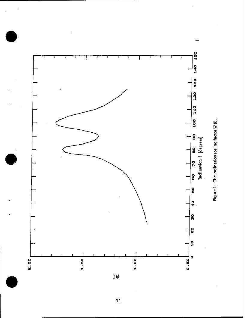
1 The inclination scaling factor 'I (i) ................................................... 11

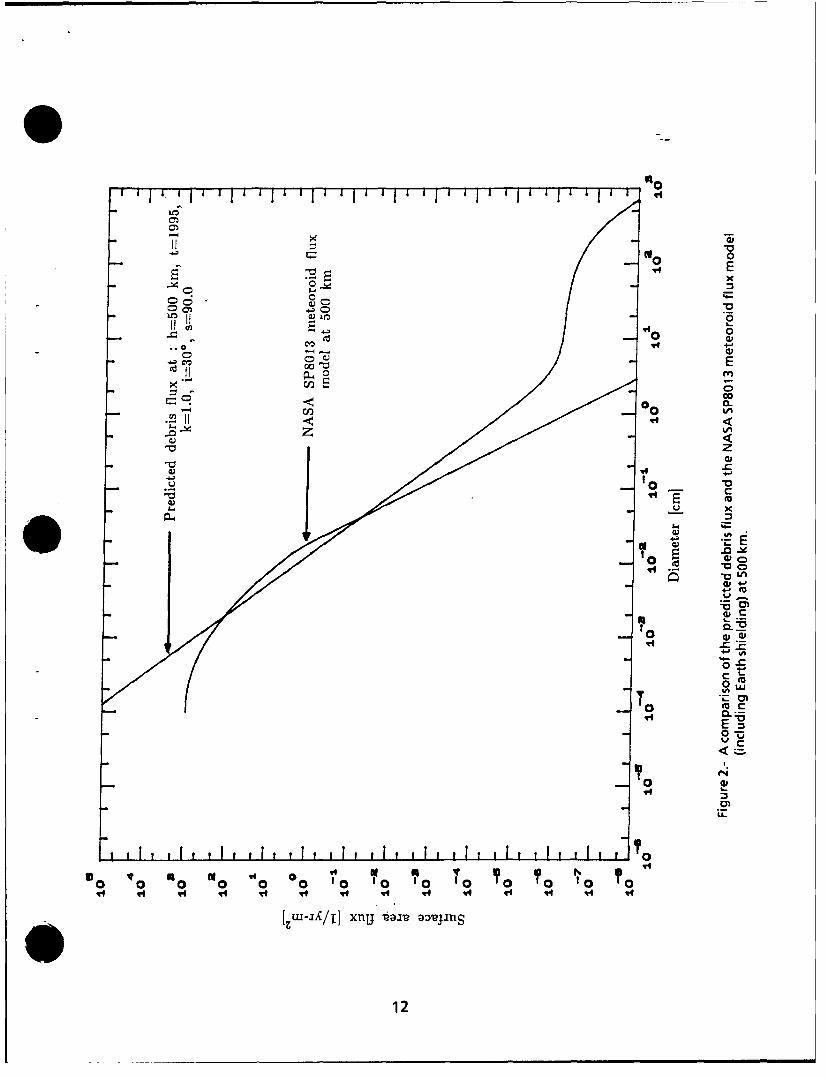
2 A comparison of the predicted debris flux and the NASA SP8013 meteoroidflux model (including Earth shielding) at 500 Km ..................................... 12

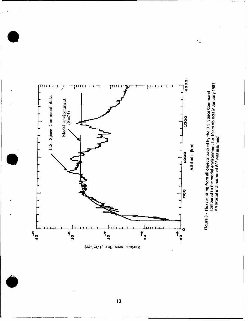
3 Flux resulting from all objects tracked by the U.S. Space Command comparedtothe model environment for 10 cm objects in January 1987. An orbitalinclination of 600 w as assum ed . ..................................................... 13

4 The un-normalized collision velocity distribution for an inclination at 300 ............... 14

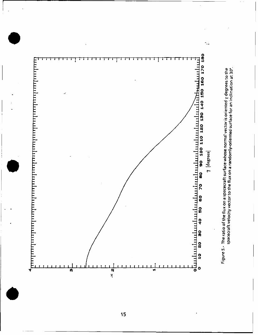
5 The ratio of flux on a spacecraft surface whose normal vector is oriented- degrees to the spacecraft velocity vector to the flux on a randomly-orientedsurface for an inclination at 30. ..................................................... 15

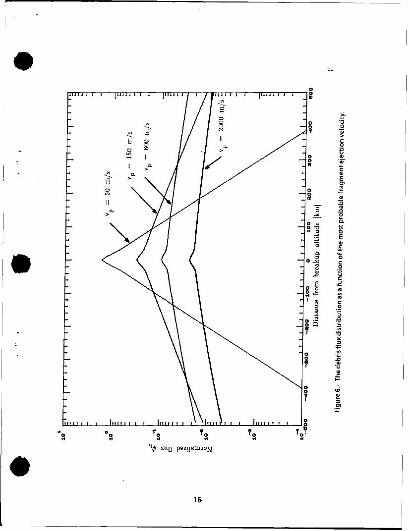
6 The debris flux distribution as a function of the most probable fragmentejection velocity ................ ................................................ . 16

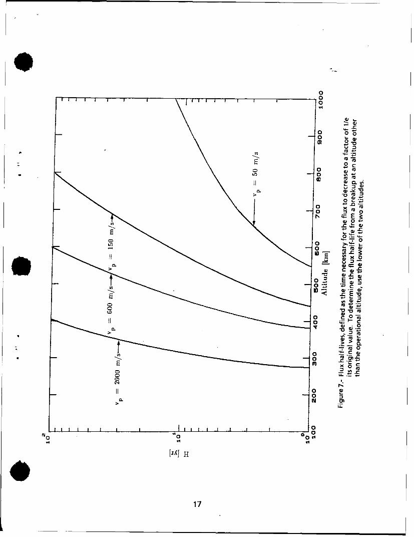
7 Flux half-lives, defined as the time necessary for the flux to decrease to a factorof l/e its original value. To determine the flux half-life from a breakup at analtitude other than the operational altitude, use the lower of the two altitudes .......... 17

0V

ABSTRACT

The orbital debris environment model contained in this report is intended to be used by the space-craft community for the design and operation of spacecraft in low Earth orbit. This environment,when combined with material-dependent impact tests and spacecraft failure analysis, is intended tobe used to evaluate spacecraft vulnerability, reliability, and shielding requirements. The environ-ment represents a compromise between existing data to measure the environment, modeling of thisdata to predict the future environment, the uncertainty in both measurements and modeling, andthe need to describe the environment so that various options concerning spacecraft design andoperations can be easily evaluated.

INTRODUCTION

The natural meteoroid environment has historically been a design consideration for spacecraft.Meteoroids are part of the interplanetary environment and sweep through Earth orbital space at anaverage speed of 20 km/s. At any one instant, a total of 200 kg of meteoroid mass is within 2000 kmof the Earth's surface. Most of this mass is concentrated in 0.1 mm meteoroids.

Within this same 2000 km above the Earth's surface, however, is an estimated 3,000,000 kg of man-made orbiting objects. These objects are in mostly high inclination orbits and sweep past oneanother at an average speed of 10 km/s. Most of this mass is concentrated in approximately 3000spent rocket stages, inactive payloads, and a few active payloads. A smaller amount of mass,approximately 40,000 kg, is in the remaining 4000 objects currently being tracked by U.S. SpaceCommand radars. Most of these objects are the result of more than 90 on-orbit satellite fragmenta-tions. Recent ground telescope measurements of orbiting debris combined with analysis of hyper-. velocity impact pits on the returned surfaces of the Solar Maximum Mission satellite indicate a totalmass of approximately 1000 kg for orbital debris sizes of 1 cm or smaller, and approximately 300 kgfor orbital debris smaller than 1 mm. This distribution of mass and relative velocity is sufficient tocause the orbital debris environment to be more hazardous than the meteoroid environment tomost spacecraft operating in Earth orbit below 2000 km altitude.

Mathematical modeling of this distribution of orbital debris predicts that collisional fragmentationwill cause the amount of mass in the 1 cm and smaller size range to grow at twice the rate as theaccumulation of total mass in Earth orbit. Over the past 10 years, this accumulation has increased atan average rate of 5 percent per year, indicating that the small sizes should be expected to increaseat 10 percent per year. Reasons that both of these rates could be either higher or lower, as well asother uncertainties in the current and projected environment, are discussed in the section "Uncer-tainty in Debris Flux." As new data become available, a new environment will be issued.

The authors wish to acknowledge those responsible for original research and data analyses utilizedby this work. Dr. Andrew Potter, Mr. John Stanley, Dr. Karl Henize, Dr. Faith Vilas, and Mr. EugeneStansbery (all at NASA/JSC) obtained and analyzed data obtained using optical telescopes, infraredtelescopes, and radar on individual debris fragments. These data were used to evaluate therelationship between the physical size, radar cross-section, and optical brightness. Dr. GautamBadhwar (NASA/ JSC) analyzed the atmospheric drag characteristics of individual fragments toevaluate the relationship between physical size and mass. Dr. David McKay (NASA/JSC) and Mr. RonBernhard (LESC) analyzed and compiled much of these impact data on the recovered surfaces fromthe Solar Maximum Mission (SMM) satellite.

01

. DATA SOURCES

The following data sources were considered in the construction of this environmental model:

1. Orbital element sets supplied by the U.S. Space Command (both the cataloged population andthose objects awaiting cataloging) for the period between 1976 and 1988

2. Optical measurements by the Massachusetts Institute of Technology (MIT) in 1984 using thetelescopes of their experimental test site (ETS) in Socorro, New Mexico

3. Measurements designed to determine orbital debris particle albedo using a ground-basedinfrared telescope at the Air Force Maui Optical Station/Maui Optical Tracking and IdentificationFacility (AMOS/MOTIF), U.S. Space Command radars, and both NASA and U.S. Space Commandtelescopes

4. Analysis of hypervelocity impacts on the surfaces returned by the Shuttle from the repaired SolarMaximum Mission satellite in 1984

5. Mathematical models which consider various traffic models and satellite fragmentationprocesses to predict the future accumulation of debris

KEY ASSUMPTIONS AND CONCLUSIONS CONCERNING DATA SOURCES

The following assumptions and/or conclusions were made or reached concerning the above datasources:

1. The flux resulting from the U.S. Space Command orbital element sets is complete to a limitingsize of 10 cm for objects detected below 1000 km altitude.

2. During average seeing conditions, the MIT telescopes detected objects to a limiting size of 5 cmin diameter at a rate of two times the rate of 10 cm and larger objects.

3. During optimum seeing conditions, the MIT telescopes detected objects to a limiting size of 2 cmin diameter at a rate of five times the rate of 10 cm and larger objects.

4. The surfaces of the Solar Maximum Mission satellite experienced an orbital debris flux whichvaries from 20 percent of the meteoroid flux for debris sizes larger than 0.05 cm to a factor of1000 times the meteoroid flux for sizes larger than 1 pm.

5. The orbital debris flux between 0.05 cm and 2 cm can be obtained by a linear interpolation (on aloglo F (flux) vs loglo d (diameter) plot) of the Solar Maximum Mission satellite surface data andthe MIT telescope data.

6. For any given size of orbital debris, the variation of flux with altitude, solar activity, orbitalinclination, and the velocity and direction distribution is the same as that predicted by the U.S.Space Command orbital element set data.

7. The accumulation of objects tracked by the U.S. Space Command, when averaged over an11-year solar cycle, will increase at a rate of 5 percent per year.

8. The accumulation of objects detected by the MIT telescopes and the Solar Maximum Missionsatellite surfaces, when averaged over an 11- year solar cycle, will increase at twice the rate ofthe tracked objects, or 10 percent per year.

2

DESIGN STANDARDS

Recommended Flux for Orbital Debris

The cumulative flux of orbital debris of size d and larger on spacecraft orbiting at altitude h,inclination i, in the year t, when the solar activity for the previous year is 5, is given by the followingequation:

F (d,h,i,t,S) = k p (h,S). w(i) -[F1 (d) "g, (t) + F2 (d) -g 2 (t)] (1)

where

F = flux in impacts per square meter of surface area per yeark = 1 for a randomly tumbling surface; must be calculated for a directional surfaced = orbital debris diameter in cmt = time expressed in yearsh = altitude in km (h % 2000 km)S = 13-month smoothed 10.7 cm-wavelength solar flux expressed in 104 Jy; retarded by 1 year

from ti = inclination in degrees

and

4(h,S) = (p, (h,S)/(41l (h,S) + 1)

41 (h,S) = 1 0(h/200- S/140- 1.5)

. F,(d) = 1.05x10-5-d-2.5

F2 (d) = 7.0 x 1010- (d + 700)-6

p = the assumed annual growth rate of mass in orbit,

gl (t) = (1 + 2. p) (t- 1985)

g 2 (t) = (1+p) (t- 1985)

The inclination-dependent function ii is a ratio of the flux on a spacecraft in an orbit of inclination ito that flux incident on a spacecraft in the current population's average inclination of approximately600. Values for q are given in figure 1 and tabulated in table 1.

An average 11-year solar cycle has values of S which range from 70 at solar minimum to 150 at solarmaximum. However, the current cycle, which peaks in the year 1990, is predicted to be aboveaverage, possibly exceeding 200.

An example orbital debris flux is compared with the meteoroid flux from NASA SP8013 in figure 2 forh = 500 km, t = 1995 years, k = 1.0, i = 300, and S = 90.0.

S

The flux is defined such that the average number of impacts N on a spacecraft surface area of Aexposed to the environment for the interval ti to tf is given by the following equation:

tf

N = Jf F.Adt (2)

ti

where A is the surface area exposed to the flux F at time t.

The value of k can theoretically range from 0 to 4 (a value of 4 can only be achieved when a surfacenormal vector is oriented in the direction of a monodirectional flux), and depends on the orientationof A with respect to the Earth and the spacecraft velocity vector. If the surface is randomly oriented,then k = 1. If the surface is oriented with respect to the Earth, then the section "Velocity andDirection Distribution" must be used to calculate a value for k. In general, if the surface area isfacing in the negative velocity direction, k = 0. However, if this area is facing in the same directionas the spacecraft velocity vector, and the spacecraft orbital inclination is near polar (which causesmore "head-on" collisions), then k will approach its maximum value of approximately 3.5 forthecurrent directional distribution.

The probability of exactly n impacts occurring on a surface is found from Poisson statistics, or

Pn Nn . e-N (3)n-T.

. Uncertainty in Debris Flux

Factors which contribute significantly to the uncertainty in the orbital debris environment areinadequate measurements, an uncertainty in the level of future space activities, and the statisticalcharacter of major debris sources. The environment has been adequately measured by groundradars for orbital debris sizes larger than 10 cm. A limited amount of data using ground telescopeshas shown a 2 cm flux which is currently estimated to be known within a factor of 3. Orbital debrissizes smaller than .05 cm have only been measured at 500 kin; at this altitude and for these smallersizes, the environment is known within a factor of 2. Interpolation was used to obtain the fluxbetween 0.05 cm and 2 cm at 500 km, and would be justified if the amount of mass between thesetwo sizes were approximately the same asthe mass contributing to the two sizes, or approximately100 kg to 1000 kg. Mathematical modeling of various types of satellite breakups in Earth orbit makesuch an assumption seem reasonable. However, other than "reasonableness," there are no datawhich would prevent the flux of any particle in the size range between 0.05 cm and 2 cm from beingas high as the 0.05 cm flux, or as low as the 2 cm flux, that is, vary by as much as several orders ofmagnitude.

An additional uncertainty from the measurements arises because there are no measurements ofdebris smaller than 2 cm at other than 500 km altitude. Mathematical modeling concludes that if thedebris is in near circular orbits and the source of the debris is at higher altitudes, the ratio of theamount of small debris to large debris should decrease with decreasing altitude. This ratio isassumed constant in the design environment. Consequently, there would be a smaller flux of lessthan 2 cm debris at altitudes less than 500 kin, and a larger flux at altitudes above 500 km than ispredicted by this model. However, if the debris is in highly elliptical orbits, then the flux of smalldebris could be nearly independent of altitude. Consequently, the amount that the flux differs fromthe design environment could be as high as a factor of 10 (either higher or lower) for every 200 km. away from the 500 km altitude, up to an altitude of approximately 700 km. The large number ofbreakups at altitudes between 700 km and 1000 km and at 1500 km, together with the extremely

4

long orbital lifetimes of fragments in these regions, make any predictions very sensitive to the natureof each of these breakups. The U.S. Space Command data give fluxes at 800 km and 1000 km which

are twice as high as predicted by the recommended flux model, as shown in figure 3. For mostaltitudes between 1000 km and 2000 kin, the current flux from objects tracked by the U.S. SpaceCommand is significantly lower than the design environment. However, the large number ofbreakups at 1500 km could have scattered smaller fragments over this region; in addition, futuretraffic may increase the flux of larger objects.

Predicting future activity in space is highly uncertain. Since 1966, the non-U.S. launch rate hasincreased by a average of 10 percent per year; however, U.S. launch rates have decreased at thissame rate, leading to a constant world launch rate since 1966. This constant launch rate has led to alinear, or decreasing percentage, growth in the accumulation of objects being tracked by the U.S.Space Command. Averaged over the last solar cycle, this accumulation has grown at an average rateof 5 percent per year. A continued constant launch rate would mean that the value of "p" in theexpression for g2 could either decrease from 0.05 with time, orthe growth rate could follow thelinear functional form g2(t) = 1 + p- (t - 1985). On the other hand, traffic models which represent thebest current estimate of future space activities up to the year 2010, would lead to between a5 percent and 10 percent per year increase in the amount of U.S. mass to orbit. In addition, someU.S. and world traffic projections would give rise to increases in the accumulation of larger objects inorbit as high as 20 percent per year. While such large increases do not seem historically justified, anupper limit of a 10 percent increase per year, or p = 0.1, is not unrealistic. Any larger increases in theuse of low Earth orbit would likely include different operational techniques which would invalidateassumptions used to express the design environment.

Predicting the population not tracked bythe U.S. Space Command is even more uncertain since we. do not even have historical data to extrapolate. However, there are some indicators. Historically,the satellite fragmentation rate has increased with time, indicating that values for g, would increasewith time faster than values for g2. However, actions are currently underway which should reducethe future satellite explosion rate. On the other hand, mathematical models predict that within thevery near future, random collisions could become an important cause of satellite fragmentations.Under these conditions, the small debris population would increase at approximately twice thepercentage rate of the large population, until a "critical density" of large objects is reached. Thiscritical density'corresponds to a value of g2 between 10 and 100 (i.e., the tracked population is 10 to100 times its 1985 total number). At thistime, values for g1 would increase very rapidly with time,independent of values for g2-

The design environment assumes that the value of g, increases at twice the percentage rate of g2.This could be expected if the satellite explosion rate continues to increase over the next decade ortwo. After this time random collisions would cause the rate to continue, independent of actions toreduce the explosion frequency. For values of p greater than 0.1, random collisions would becomeimportant in less than a decade, again consistent with the environment assumption. However, if theexplosion rate is immediately reduced, and the current rate at which mass is placed into orbit doesnot significantly increase, then the design environment will predict fluxes for debris sizes smallerthan 10cm over the next 10 to 20 years which are too high by a factor of 2 to 10.

Average Mass Density

The average mass density for debris objects 1 cm in diameter and smaller is 2.8 g/cm 3. The averagemass density for debris larger than 1 cm is based on observed breakups, area-to-mass calculations. derived from observed atmospheric drag, ground fragmentation tests, and known intact satellitecharacteristics.

5

This density has been found to fit the following relationship:

p = 2.8. d-0.74 (4)

Velocity and Direction Distribution

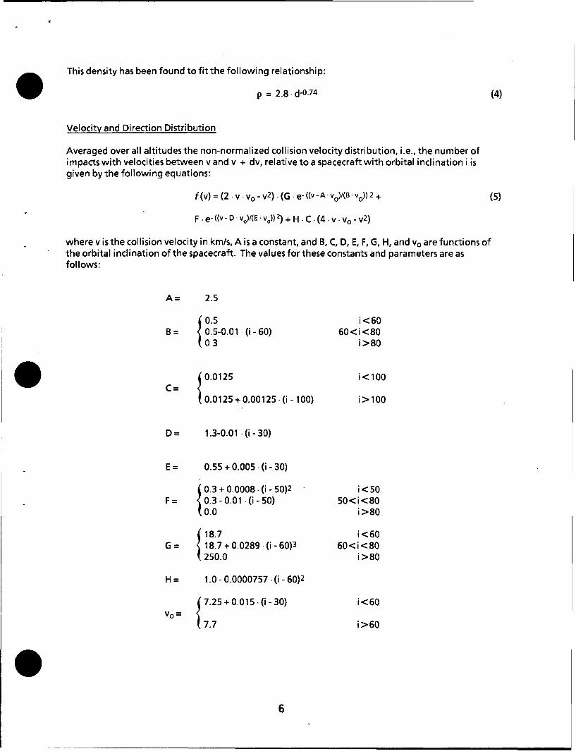
Averaged overall altitudesthe non-normalized collision velocity distribution, i.e., the number ofimpacts with velocities between v and v + dv, relative to a spacecraft with orbital inclination i isgiven by the following equations:

f(v)=(2. v.vo-v 2). (G .e-((v- A Vo)/(B.Vo))2+ (5)

F . e- ((v - D. vo)/(E Vo)) 2) + H -C -(4- v . Vo - v 2 )

where v is the collision velocity in km/s, A is a constant, and B, C, D, E, F, G, H, and vo are functions ofthe orbital inclination of the spacecraft. The values for these constants and parameters are asfollows:

A= 2.5

0.5 i<60B 0.5-0.01 (i - 60) 60<i<80

103 i>80

0= t0.0125 i<100

0.0125 + 0.00125. (i - 100) i>100

D= 1.3-0.01 • (i - 30)

E= 0.55 + 0.005. (i - 30)

0.3 + 0.0008- (i - 50)2 i<50F= 0.3- 0.01 .(i- 50) 50<i<80

0.0 i >80

18.7 i<60G= 18.7 + 0.0289. (i - 60)3 60<i<80

250.0 i>80

H = 1.0 - 0.0000757- (i - 60)2

V 7.25+0.015.(i-30) i<60

!= 17.7 i >60

06

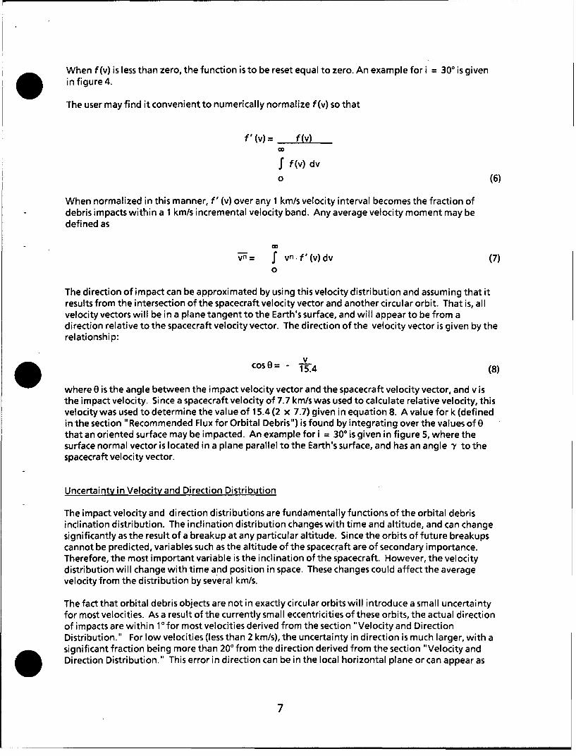
When f(v) is less than zero, the function is to be reset equal to zero. An example for i = 300 is givenin figure 4.

The user may find it convenient to numerically normalize f(v) so that

f' (v)= f (v)

f f(v) dv

0 (6)

When normalized in this manner, f' (v) over any 1 km/s velocity interval becomes the fraction ofdebris impacts within a 1 km/s incremental velocity band. Any average velocity moment may bedefined as

v7= f vn.f'(v)dv (7)

0

The direction of impact can be approximated by using this velocity distribution and assuming that itresults from the intersection of the spacecraft velocity vector and another circular orbit. That is, allvelocity vectors will be in a plane tangent to the Earth's surface, and will appear to be from adirection relative to the spacecraft velocity vector. The direction of the velocity vector is given by therelationship:

V

cosO= - 15.4 (8)

where 0 is the angle between the impact velocity vector and the spacecraft velocity vector, and v is

the impact velocity. Since a spacecraft velocity of 7.7 km/s was used to calculate relative velocity, thisvelocity was used to determine the value of 15.4 (2 x 7.7) given in equation 8. A value for k (definedin the section "Recommended Flux for Orbital Debris") is found by integrating over the values of 0that an oriented surface may be impacted. An example for i = 300 is given in figure 5, where thesurface normal vector is located in a plane parallel to the Earth's surface, and has an angle -Y to thespacecraft velocity vector.

Uncertainty in Velocity and Direction Distribution

The impact velocity and direction distributions are fundamentally functions of the orbital debrisinclination distribution. The inclination distribution changes with time and altitude, and can changesignificantly as the result of a breakup at any particular altitude. Since the orbits of future breakupscannot be predicted, variables such as the altitude of the spacecraft are of secondary importance.Therefore, the most important variable is the inclination of the spacecraft. However, the velocitydistribution will change with time and position in space. These changes could affect the averagevelocity from the distribution by several km/s.

The factthat orbital debris objects are not in exactly circular orbits will introduce a small uncertaintyfor most velocities. As a result of the currently small eccentricities of these orbits, the actual directionof impacts are within 10 for most velocities derived from the section "Velocity and DirectionDistribution." For low velocities (less than 2 km/s), the uncertainty in direction is much larger, with asignificant fraction being more than 200 from the direction derived from the section "Velocity andDirection Distribution." This error in direction can be in the local horizontal plane or can appear as

7

direction errors above or below this plane. High velocity impacts will almost always occur very nearto the local horizontal plane and from the forward (downrange) direction; low speed impacts canoccur from almost any angle (00 - angle < 1800) in the local horizontal plane as well as atconsiderable angles (0° - angle - 900) out of that plane.

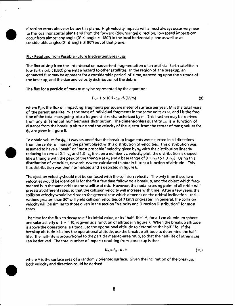
Flux Resulting from Possible Future Inadvertent Breakups

The flux arising from the intentional or inadvertent fragmentation of an artificial Earth satellite inlow Earth orbit (LEO) presents a hazard to other satellites. In the region of the breakup, anenhanced flux may be apparent for a considerable period of time, depending upon the altitude ofthe breakup, and the size and velocity distribution of the debris.

The flux for a particle of mass m may be represented by the equation:

Fb = 1 x 10-9. 4b -f (M/m) (9)

where Fb is the flux of impacting fragments per square meter of surface per year, M is the total massof the parent satellite, m is the mass of individual fragments in the same units as M, and f is the frac-tion of the total mass going into a fragment size characterized by m. This fraction may be derivedfrom any differential number/mass distribution. The dimensionless quantity 4b is a function ofdistance from the breakup altitude and the velocity of the ejecta from the center of mass; values for

IN are given in figure 6.

To obtain values for 4)b, it was assumed that the breakup fragments were ejected in all directionsfrom the center of mass of the parent object with a distribution of velocities. This distribution was. assumed to have a "peak" or "most probable" velocity given by vp with the distribution linearlyreducing to zero at 0.1 vp and 13. vp (i.e., on a number vs. velocity plot, the distribution is shapedlike a triangle with the peak of the triangle at vp and a base range of 0.1 vp to 1.3 . vp). Using thisdistribution of velocities, new orbits were calculated to obtain flux as a function of altitude. Thisflux distribution was then normalized and is depicted in figure 6.

The ejection velocity should not be confused with the collision velocity. The only time these twovelocities would be identical is for the first few days following a breakup, and the object which frag-mented is in the same orbit as the satellite at risk. However, the nodal crossing point of all orbits willprecess at different rates, so that the collision velocity will increase with time. After a few years, thecollision velocity would be close to the general case which depends on the orbital inclination. Incli-nations greater than 300 will yield collision velocities of 7 km/s or greater. In general, the collisionvelocity will be similar to those given in the section "Velocity and Direction Distribution" for mostcases.

The time for the flux to decay to e-1 its initial value, or its "half- life" H, for a 1 cm aluminum sphereand solar activity of S = 110, is given as a function of altitude in figure 7. When the breakup altitudeis above the operational altitude, use the operational altitude to determine the half-life. If thebreakup altitude is below the operational altitude, use the breakup altitude to determine the half-life. The half-life is proportional to the particle mass-to-area ratio, so that the half-life of other sizescan be derived. The total number of impacts resulting from a breakup is then

Nb= Fb-A H (10)

where A is the surface area of a randomly oriented surface. Given the inclination of the breakup,. both velocity and direction could be derived.

8

DISCUSSION: AN EXAMPLE OF A FUTURE BREAKUP

When a satellite breaks up in space, its size and velocity distribution are a sensitive function of the

type of breakup. If it were a low intensity explosion, nearly all of the fragment mass would be insizes larger than approximately 10 cm, and the most probable ejection velocity would likely beapproximately 50 m/s. The fragments from a hypervelocity collision would include a significantfraction of mass with sizes less than 10 cm. However, the most probable velocities of these frag-ments would increase with decreasing size. Most of the fragments from a high intensity explosioncould go into almost any preferred size, depending on the nature of the explosion.

As an example, assume that half of the mass from a 1000 kg satellite goes into 1 cm fragments. Also,assume that the satellite fragmented at an altitude of 600 km, and that the probable ejectionvelocity was 150 m/s. The resulting flux of 1 cm fragments at 500 km would be 5 x 10-5 impacts/m 2 -yr.This is larger (by several factors) than the flux predicted at 500 km for 1995, given in the section"Recommended Flux for Orbital Debris." However, assuming no additional breakups occur, thislarger flux will effectively last for only 3 years, as shown in figure 7.

REFERENCES

Many of the assumptions and analyses in this report are based upon unpublished work conducted bythe Solar System Exploration Division at NASA's Lyndon B. Johnson Space Center, and upon theunpublished orbital element sets provided by the U.S. Space Command. Published material whichcould provide the reader additional background material can be found in the following references:. D. J. Kessler, E. Gran, and L. Sehnal, eds., Space Debris, Asteroids, and Satellite Orbits, Advances

Space Res. 5, No. 2, 1985, pp. 3-94.

J. A. M. McDonnell, M. S. Hanner, and D. J. Kessler, eds., Cosmic Dust and Space Debris, AdvancesSpace Res. 6, No. 2, 1986, pp. 97-158.

N. L Johnson and D. S. McKnight. Artificial Space Debris. Malabar, Florida: Orbit Book Company,1987.

Aerospace America 26, No. 6, June 1988, pp. 8-10, 16-25.

Johnson, N. L. History and Projections of Foreign Satellite Mass to Earth Orbit. Teledyne BrownEngineering (Colorado Springs, Colorado), CS86-USASDC-0015, July 31, 1986.

Space Transportation Plans and Architecture Directorate. DoD Space Transportation MissionRequirements Definition, Vol. I: Discussion. The Aerospace Corporation, (El Segundo, California),TOR-0086A(2460-01)-i, December 12, 1986.

R. Kadunc and D. R. Branscome/Code MD. Civil Needs Data Base, Vers. 3.0, Vol. I - ExecutiveSummary. Washington, D. C.: NASA Headquarters, February 5, 1988.

9

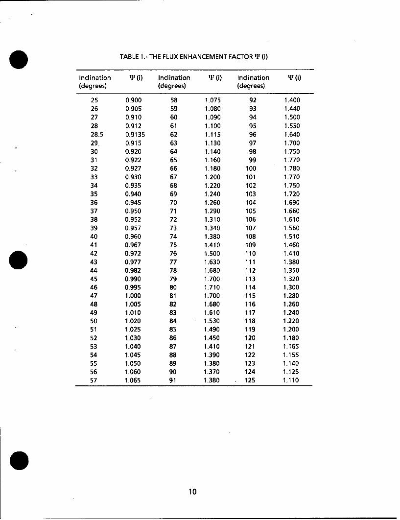
TABLE 1.- THE FLUX ENHANCEMENT FACTOR W (i)

Inclination • (i) Inclination (i) Inclination W(i)(degrees) (degrees) (degrees)

25 0.900 58 1.075 92 1.40026 0.905 59 1.080 93 1.44027 0.910 60 1.090 94 1.50028 0.912 61 1.100 95 1.55028.5 0.9135 62 1.115 96 1.64029 0.915 63 1.130 97 1.70030 0.920 64 1.140 98 1.75031 0.922 65 1.160 99 1.77032 0.927 66 1.180 100 1.780

33 0.930 67 1.200 101 1.77034 0.935 68 1.220 102 1.75035 0.940 69 1.240 103 1.72036 0.945 70 1.260 104 1.69037 0.950 71 1.290 105 1.66038 0.952 72 1.310 106 1.61039 0.957 73 1.340 107 1.56040 0.960 74 1.380 108 1.51041 0.967 75 1.410 109 1.46042 0.972 76 1.500 110 1.410

43 0.977 77 1.630 111 1.38044 0.982 78 1.680 112 1.35045 0.990 79 1.700 113 1.32046 0.995 80 1.710 114 1.30047 1.000 81 1.700 115 1.28048 1.005 82 1.680 116 1.26049 1.010 83 1.610 117 1.24050 1.020 84 1.530 118 1.22051 1.025 85 1.490 119 1.20052 1.030 86 1.450 120 1.18053 1.040 87 1.410 121 1.16554 1.045 88 1.390 122 1.15555 1.050 89 1.380 123 1.14056 1.060 90 1.370 124 1.12557 1.065 91 1.380 125 1.110

10

0

0

0

0'4

00

0'44'cc

boo m

Nv

'42-0 -

00 0

Woo* Oo o

II-

0

00

W E >

oo~0 Q)0 ~ m.5

0� E

II E0 -m"4

0014

,.o l i t€ l i •1 1 i i l t l t l t t l I I 1 0

-0 0 00-

-~ U

15. Tq4-v

[,tu-iX/T xni ýax a:.-j.-

0

.U '

120

00

CA.

UCC

oor. U.4-

-i

00o0-

0~j

o 4--Z 0

0~ ---.

s. 40..c

=-0

L..

To0 T 00 ToT0T1 q4 'f 4 '4

13

to

mv4

0

c

Vf .0

.C

F-.

m 1..

0 0n

(AUl

14U

0

0M 0

oo

0 0>.C

oo

•c

oo!o010

x1

M0

154

0 00ovo -q)

0 IV

V4- >

o0

00

U))w

00

15

0

0

CD c

C .0

V3 v

0 ~00

"r-

C 00 0

44-

0

I mc

0 00

if, 0

0~

00

_U.100

160

00

10

GDL)

0 ..o

0 0

EE

0 4-40 0

0 kI 00

x0

o3

g-0""'Ov%n 4,

76D.0D~-G

o~ Eo

0 00

m -

00

0

:117

REPORT DOCUMENTATION PAGE

1. Report No. 2. Government Accession No. 3. Recipient's Catalog No.

TM-100471

11lTitle and Subtitle 5. Report Date

Orbital Debris Environment for Spacecraft Designed to Operate in Low Earth April 1989

Orbit 6. Performing Organization Code

7. Author(s)8. Performing Organization Report No.

Donald J. Kessler, Robert C. Reynolds, and Phillip D. Anz-Meador S-588

9. Performing Organization Name and Address 10. Work Unit No.

Lyndon B. Johnson Space CenterHouston, Texas 77058 11. Contract or Grant No.

12. Sponsoring Agency Name and Address 13. Type of Report and Period CoveredTechnical Memorandum

National Aeronautics and Space AdministrationWashington, DC 20546 14. Sponsoring Agency Code

15. Supplementary Notes

Donald J. Kessler/SN3, NASA-Lyndon B. Johnson Space Center, Houston, Texas 77058Robert C. Reynolds & Phillip D. Anz-Meador/C23, Lockheed Engineering & Sciences Co.,

* 400 NASA Rd. 1, Houston, Texas 77058*.JAbstr~act

The orbital debris environment model contained in this report is intended to be used by the spacecraft communityfor the design and operation of spacecraft in low Earth orbit. This environment, when combined with material-dependent impact tests and spacecraft failure analysis, is intended to be used to evaluate spacecraft vulnerability,reliability, and shielding requirements. The environment represents a compromise between existing data tomeasure the environment, modeling of these data to predict the future environment, the uncertainty in bothmeasurements and modeling, and the need to describe the environment so that various options concerning

. spacecraft design and operations can be easily evaluated.

17. Key Words (Suggested by Author(s)) 18. Distribution Statement

Debris Hazards Unclassified - UnlimitedCollisions Environment Models

xplosions MeteoroidsSubject Category: 12

19. Security Classification (of this report) 20. Security Classification (of this page) 21. No. of pages 22. Price

Unclassified Unclassified 22

For sale by the National Technical Information Service, Springfield, VA 22161-2171 NASA-JSC

JSC Form 1424 (Rev Jan 88) (Ethernet Jan 88)