Orbital Consequences from the Giant Impact Theory Consequences from the Giant Impact Theory by ......
58
Orbital Consequences from the Giant Impact Theory by Anthony Hales A senior thesis submitted to the faculty of Brigham Young University-Idaho in partial fulfillment of requirements for a degree of Bachelor of Science Department of Physics Brigham Young University-Idaho April 2015
Transcript of Orbital Consequences from the Giant Impact Theory Consequences from the Giant Impact Theory by ......
Orbital Consequences from the Giant Impact Theory
by
Anthony Hales
A senior thesis submitted to the faculty of Brigham Young University-Idaho in partial
fulfillment of requirements for a degree of Bachelor of Science
Department of Physics
Brigham Young University-Idaho
April 2015


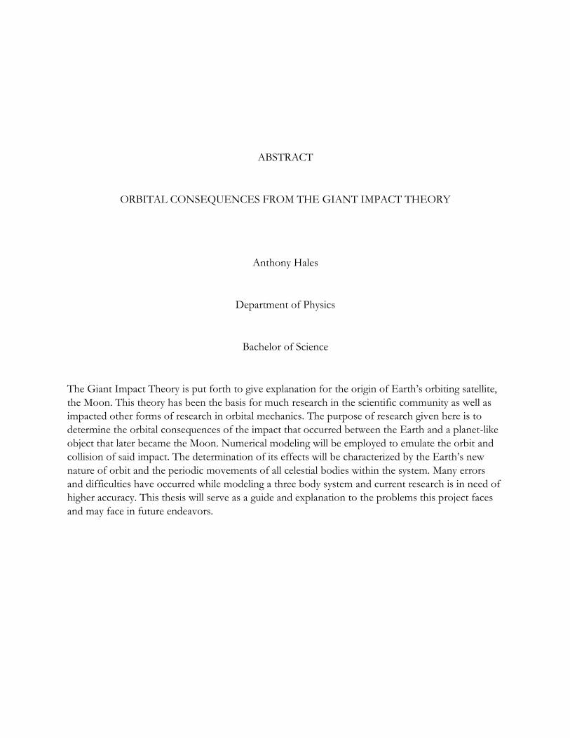
ABSTRACT
ORBITAL CONSEQUENCES FROM THE GIANT IMPACT THEORY
Anthony Hales
Department of Physics
Bachelor of Science
The Giant Impact Theory is put forth to give explanation for the origin of Earth’s orbiting satellite,
the Moon. This theory has been the basis for much research in the scientific community as well as
impacted other forms of research in orbital mechanics. The purpose of research given here is to
determine the orbital consequences of the impact that occurred between the Earth and a planet-like
object that later became the Moon. Numerical modeling will be employed to emulate the orbit and
collision of said impact. The determination of its effects will be characterized by the Earth’s new
nature of orbit and the periodic movements of all celestial bodies within the system. Many errors
and difficulties have occurred while modeling a three body system and current research is in need of
higher accuracy. This thesis will serve as a guide and explanation to the problems this project faces
and may face in future endeavors.

ACKNOWLEDGEMENTS
I would like to give thanks to my advisor, Dr. Brian Tonks, who helped me understand this research
project as well as spending many office hours problem solving the difficulties we were having. I also
want to express my gratitude for David Oliphant and the rest of the staff in the Department for
guiding me in my error analysis and corrections to the programming code. Finally, I would like to
thank my wife and family for supporting me through many of those sleepless nights and for being
there when I needed and audience for my research.

ix
Table of Contents
Abstract ............................................................................................................................................................... v
Acknowledgments............................................................................................................................................ vii
Table of Contents ............................................................................................................................................. ix
List of Figures .................................................................................................................................................... xi
1 Introduction ................................................................................................................................................... 1
1.1 Giant Impact Theory ..................................................................................................................... 1
1.2 Milankovitch Cycles ....................................................................................................................... 2
1.3 Argument and Purpose ................................................................................................................. 4
2 Computational Methods ............................................................................................................................ 5
2.1 Euler-Cromer.................................................................................................................................. 5
2.2 Runge-Kutta ................................................................................................................................... 7
2.3 Language Conversion .................................................................................................................... 9
3 Simulation Setup ........................................................................................................................................ 10
3.1 Three-Body Diagram ................................................................................................................... 10
3.2 Assumptions ................................................................................................................................. 12
3.3 Monte-Carlo Method .................................................................................................................. 13
4 Results ........................................................................................................................................................... 14
4.1 Eccentricity Comparisons ........................................................................................................... 14
4.2 Error Analysis ............................................................................................................................... 16
4.3 Accounting for Bias ..................................................................................................................... 19
5 Conclusion ................................................................................................................................................... 21
5.1 Interpretation ................................................................................................................................ 21
5.2 Limitations .................................................................................................................................... 22
5.3 Future Research ........................................................................................................................... 23
Bibliography ...................................................................................................................................................... 25
Appendix A—MATLAB Code...................................................................................................................... 26

xi
List of Figures
Figure 1: Axial and Orbital Precessions .......................................................................................................... 3
Figure 2: Orbital System ................................................................................................................................... 6
Figure 3: Euler vs. Runge-Kutta ...................................................................................................................... 8
Figure 4: Three-Body Diagram for Orbits ................................................................................................... 11
Figure 5: Earth’s Resulting Eccentricities ..................................................................................................... 15
Figure 6: Earth’s Eccentricities with Varying Mass .................................................................................... 17
Figure 7: Orbit Comparison between Euler-Cromer and Runge-Kutta .................................................. 18
Figure 8: Monte-Carlo Eccentricities ............................................................................................................ 20
Figure 9: Comparison of Energies ................................................................................................................ 22

1
Chapter 1
Introduction
1.1 Giant Impact Theory
The origin of Earth’s defining satellite, the Moon, has been a hot topic since the mid-
twentieth century. Three major theories of the Moon’s origin comprised this time period and were
the theories of fission, capture, and co-accretion. The theory of fission involved the rotational
velocity of a proto-earth being so high as to cause a part to be separated from the planet, and then
gather together in orbit around the Earth. The theory of capture was the idea that the Earth’s mass
was able to capture a small celestial body in proximity by its own gravitational pull. The theory of
co-accretion proposed that the Moon gradually formed from gravity acting on planetary dust that
was already in the process of lumping together to form the Earth itself orbiting around the Sun.
Simply put, the idea is that as the Earth was coalescing in the Sun’s orbit the Moon also was
coalescing in the Earth’s orbit [1].
At the time of the Apollo missions and their successful return of lunar samples to the Earth,
these three theories were put to the test to determine if any empirical data could support one theory
more than the others. The examination of the lunar samples showed high concentrations of
refractory elements (high vaporization temperature), low concentrations of volatile elements (low
vaporization temperature), and a strong depletion of iron-like elements. Knowing this lunar
composition, all three theories had predictions of the Moon’s composition that were inconsistent to
what was observed. Both capture and co-accretion would need a larger make-up of volatile elements
2
and the presence of iron-like materials. The fission theory would also need a composition similar to
that of Earth, but the concentrations of refractory elements were not and scientists were hard
pressed to explain how such concentration could occur [1]. This would allow for an open door in
which a new hypothesis could be introduced to the scientific community.
The giant impact hypothesis gained traction when proposed by scientists Hartman and Davis
in 1975, and Cameron and Ward in 1976. This hypothesis proposes that a planet-like object
impacted the Earth roughly 4.5 billion years ago. For this object to exhibit the same properties as is
now known about the Moon and its orbit, this impacting planet would have to be at least the size of
Mars before hitting Earth. Many studies and computer simulations have been carried out to
determine correct angular momentum and the Roche limits. The Roche limits are where the gravity
of both colliding objects begin to tear each other apart due to their proximity and how this affects
the initial angular momentum of the system. The modelled impacts from these studies are explaining
what could be observed for the systems element concentration and orbital characteristics for
accretion disks to occur (e.g. Cameron [2]; Canup [3]).
While much of these studies are focused on maintaining a Moon-like object in orbit around
the Earth, the research presented here will look at random impacting orbits of each Mars-like object
and their effect on the Earth’s orbit. A resulting orbit from impact will yield a specific eccentricity
for that new orbit. By using the characteristics of this new orbit for the represented Earth one can
compare how close that orbit is to observations of Earth today. Another theory that was making
gains in the scientific community during this time was the orbital calculations of the Milankovitch
Cycles. These cycles would describe an interesting characteristic of the Earth’s orbit and how they
can be incorporated into this research.
1.2 Milankovitch Cycles
3
The Milankovitch Cycles, named after the geophysicist Milutin Milanković, are the orbit and
rotational calculations made to explain historical accounts of climate change on the Earth. In 1976, a
professor of Earth and environmental sciences, James D. Hays, presented Milanković’s work to
show that the Earth precession and orbital obliquity affected climate change for 500,000 years from
ocean sediment cores obtained and analyzed [4]. There are current studies that adapt to Hays
previous research and attempt to determine how the Earth’s climate will change in time. Before
these studies, the Milankovitch Cycles were not held in high regards because of the lack in
conclusive evidence in historical climate models.
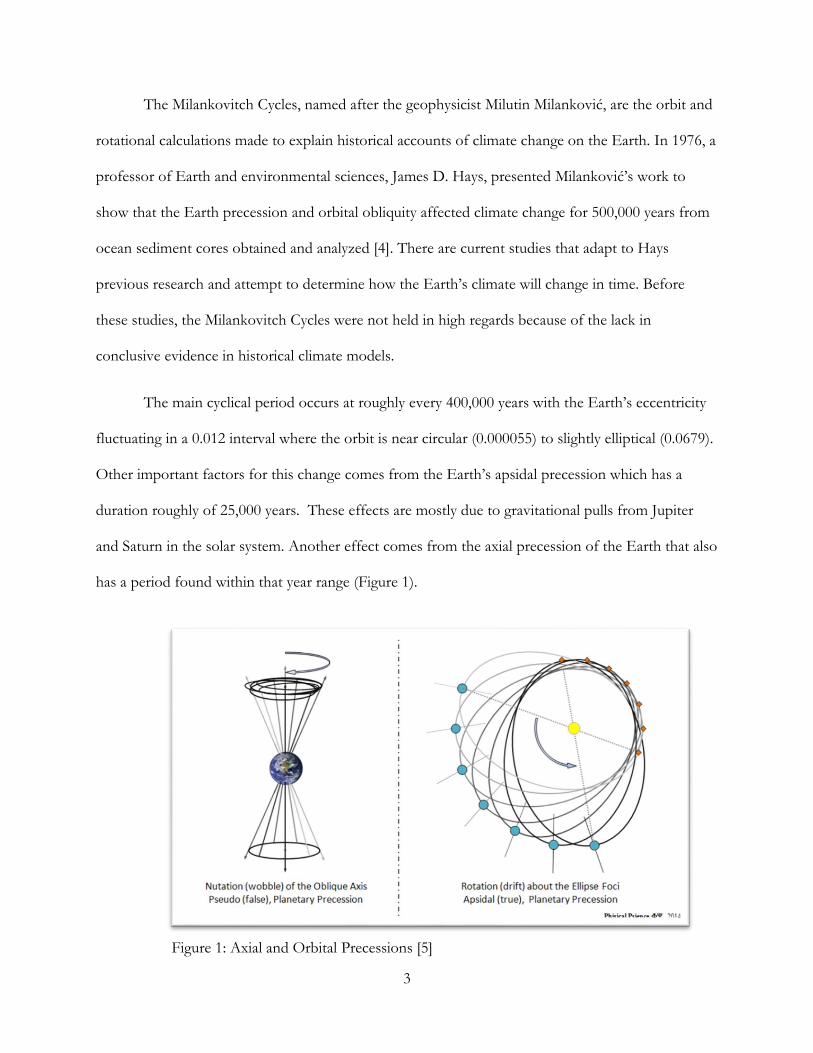
The main cyclical period occurs at roughly every 400,000 years with the Earth’s eccentricity
fluctuating in a 0.012 interval where the orbit is near circular (0.000055) to slightly elliptical (0.0679).
Other important factors for this change comes from the Earth’s apsidal precession which has a
duration roughly of 25,000 years. These effects are mostly due to gravitational pulls from Jupiter
and Saturn in the solar system. Another effect comes from the axial precession of the Earth that also
has a period found within that year range (Figure 1).
Figure 1: Axial and Orbital Precessions [5]
4
As important a topic as is the cause for global climate change, the research that is to follow
will have the goal of using the Milankovitch Cycles to determine accuracy. The initial impact and
resulting eccentricity for the Earth will be compared with the Earth’s eccentric interval to validate
the theories possibilities. With the Milankovitch Cycles and the Giant Impact Theory, we can
attempt to recreate an orbital model and determine if it closely conveys observations that the Earth
follows today by its eccentricity interval and precession. This will be under the assumption that the
Milankovitch Cycles were the same between the past and now.
1.3 Argument and Purpose
With both theories in mind, I would submit that a computational model of Earth’s orbit can
be designed to test whether such an impact falls within the interval of eccentricity and could produce
the precessive movements we view today. Questions that we can answer with such analysis is
whether the Earth’s orbit may dramatically change in which we will likely find ourselves outside the
Sun’s habitable zone. If the Earth was to change its distance by just .2 Astronomical Units, then the
planet would not be found within the Sun’s habitable zone [6]. A three body system (Earth, Sun, and
impactor) will be sufficient to show the likelihood that a resulting eccentricity within Earth’s interval
is possible. For a demonstration of the precessive movements and their periods, the inclusion of the
entire solar system will be needed.
We also may ask about the probability of such an impact occurring and how its combined
mass will affect the rest of the solar system. The combination of these theories can help us produce
more evidence for or against a general example of the Giant Impact Theory (one object, one
collision). There are additional studies that adopt parts of the current theory and apply them to old
theories (e.g. fission, capture, and co-accretion) for the Moon’s history [1].
5
Even though the exact initial conditions of the impact are unknown, an observation and
analysis of large sample orbits can be used to determine the probability of Earth’s orbit from a
planet-sized impact. With these orbits we can now stack them up to the Milankovitch Cycles and
view their probability in occurring the way our theories have outlined the proposed impacts. A
method of this simulation and its required assumptions are explained in the next chapter.
Chapter 2
Computational Methods
2.1 Euler-Cromer
The Euler-Cromer method is a slight variation of the Euler method that is used when faced
with ordinary differential equations with their initial values known. Nicholas Giordano and Hisao
Nakanishi gave detailed examples and explanation of this method in their book (p. 94-118) [7],
which is summarized hereafter. The Euler method itself is derived from the Taylor series expansion
of a position around a point in time. Suppose we have a first order differential equation as follows:
𝑑
𝑑𝑡𝑥(𝑡) = 𝑓(𝑥, 𝑡)
The initial condition is known to be 𝑥(0) = 𝑥0 and the Taylor series expansion would then be the
following:
𝑥(𝑡 + Δ𝑡) = 𝑥(𝑡) +𝑑𝑥
𝑑𝑡Δ𝑡 +
1
2
𝑑2𝑥
𝑑𝑡2(Δ𝑡)2 + ⋯
6
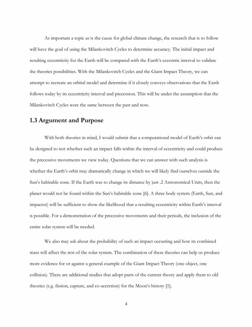
Under the Euler method, the terms of (Δ𝑡)2 and higher are dropped and is then considered
a local order of a particular approximation. The local order being the first two terms and the
particular approximation that those terms yield in the given equation. In other words, the size of the
time interval Δ𝑡 determines the accuracy of the approximation for the given function. A smaller
value of Δ𝑡 will produce smaller error in the evaluation, while a larger value could cause said
evaluation to be chaotic depending on the system (e.g. projectile, oscillatory, or rotational motion).
See Figure 2 for an orbital system with different value of Δ𝑡.
Figure 2: Orbital System
The preferred method for second order differential equations is the Euler-Cromer method.
In systems such as oscillatory motion, the Euler method is not sufficient in the conservation of total
energy in the system. This is because the Euler method relies upon the initial conditions of position
and velocity to determine (independently from one another) the new position and velocity of the
system by the given Δ𝑡. The Euler-Cromer method instead uses the initial conditions for velocity to
7
determine its future value at Δ𝑡 and uses that future value to determine its future position from its
initial position. This method is useful for simple oscillatory systems, but can still cause instability
when Δ𝑡 is not sufficiently small as shall be made apparent within this research.
2.2 Runge-Kutta
Another method to evaluate second order differential equations is the Runge-Kutta. The
Runge-Kutta method is used to incorporate the higher order terms in the Taylor series expansion
without actually solving for the partial differentials that are needed to find those orders. This is done
by using the same Euler-Cromer method to construct approximations of the higher order terms
within interval of Δ𝑡.
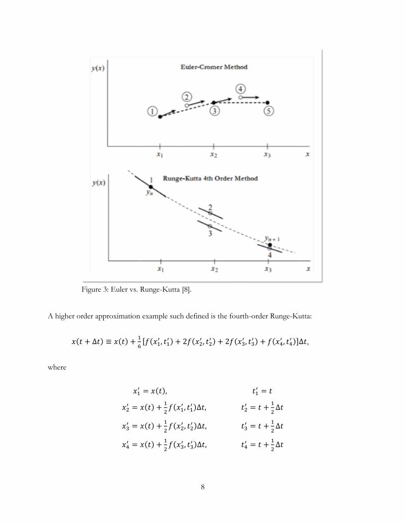
Using the orbital system in Figure 2 as an example, suppose the Δ𝑡 interval is not sufficiently
small enough to determine the exact slope and shape of the orbit. Without decreasing the size of the
interval, an approximation around this interval is needed to more accurately define the object’s
motion (See Figure 3).
8
Figure 3: Euler vs. Runge-Kutta [8].
A higher order approximation example such defined is the fourth-order Runge-Kutta:
𝑥(𝑡 + Δ𝑡) ≡ 𝑥(𝑡) +1
6[𝑓(𝑥1
′ , 𝑡1′ ) + 2𝑓(𝑥2
′ , 𝑡2′ ) + 2𝑓(𝑥3
′ , 𝑡3′ ) + 𝑓(𝑥4
′ , 𝑡4′ )]Δ𝑡,
where
𝑥1′ = 𝑥(𝑡), 𝑡1
′ = 𝑡
𝑥2′ = 𝑥(𝑡) +
1
2𝑓(𝑥1
′ , 𝑡1′ )Δ𝑡, 𝑡2
′ = 𝑡 +1
2Δ𝑡
𝑥3′ = 𝑥(𝑡) +
1
2𝑓(𝑥2
′ , 𝑡2′ )Δ𝑡, 𝑡3
′ = 𝑡 +1
2Δ𝑡
𝑥4′ = 𝑥(𝑡) +
1
2𝑓(𝑥3
′ , 𝑡3′ )Δ𝑡, 𝑡4
′ = 𝑡 +1
2Δ𝑡
9
By this approximation the evaluation time is increased by four for this interval, but the
accuracy of the calculations are now much higher than before (See Giordano [7]) as will be shown in
later chapters. The importance of decreasing the time step as the both the Earth and impactor cross
paths is paramount to producing a realistic model. While maintaining a smaller time step is
preferred, the distance between the Earth and impactor allows an indication whether to change this
time step near proximity and restore or keep the interval in the evaluation.
2.3 Language Conversion
The computational programming software chosen for this research will be MATLAB®. This
software allows users the ability to construct and quickly calculate complicated algorithms and
display detailed graphical data and models similar to Java or C++. The methods described above
(Euler-Cromer, Runge-Kutta) were written according to the programming language found within
MATLAB.
The foundation of the MATLAB language is reminiscent of C++ and one is able to read
such code with ease of an introductory level in coding. An example of such conversion can be the
line of code which states disp(X) and can be placed anywhere within the program. This part in code
is the exact same as the print option in C++ for cout(X). When transferring coding language from
one platform to another, it is best have on had a copy of the code in the previous platform and use
that as a plan for the structure in said new platform.
The conversion of this language into more robust forms of computational languages, like
C++ or Perl, is possible for future research. Such conversion would need reference material in
desired language and a complete understanding with the mechanics of functions used in the
10
MATLAB code as well. The extent of this research will be solely dedicated in MATLAB programing
language.
Chapter 3
Simulation Setup
3.1 Three-Body Diagram
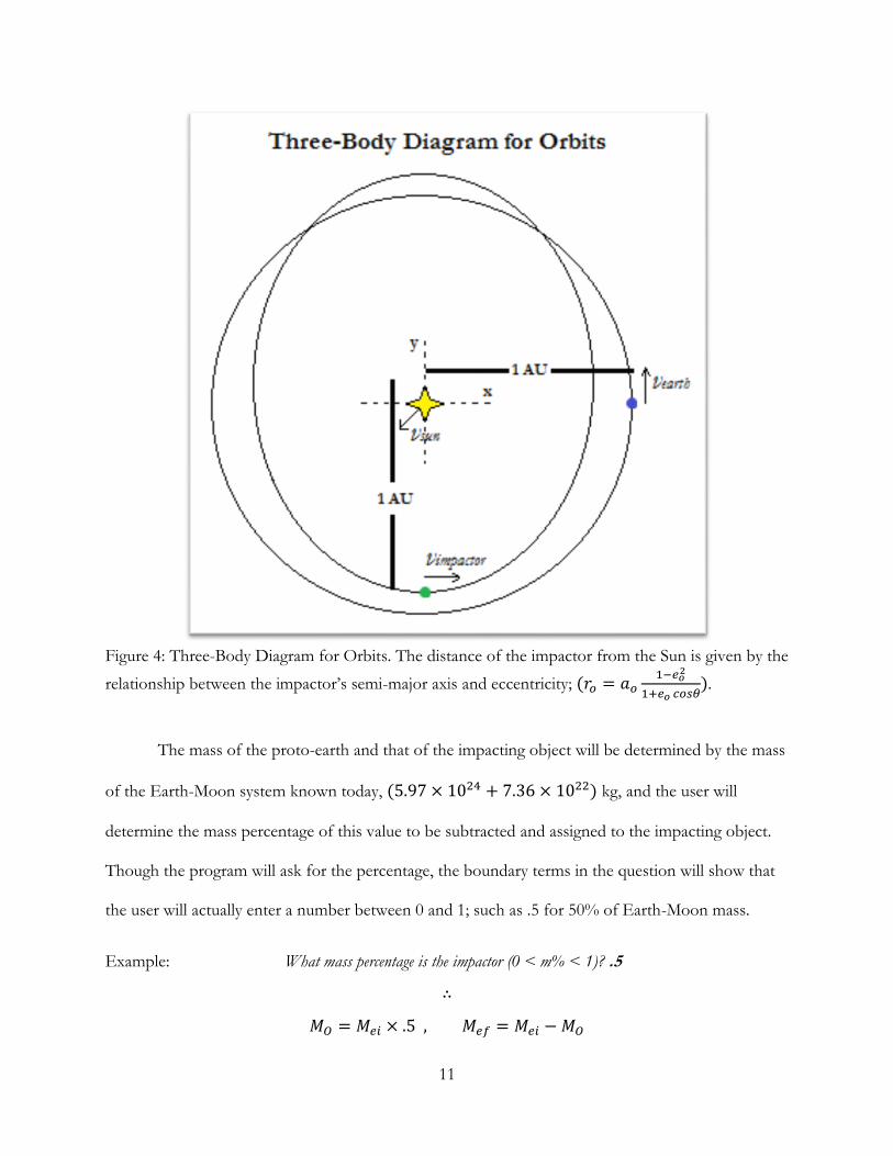
The initial setup of this planetary system will involve a three-body diagram. The Sun with
mass of 1.989 × 1030 kg will be located at the origin of our model. The proto-earth will be located
1 AU from the Sun on the x-axis with initial angle of zero. The impacting object will also be located
1 AU from the Sun, but will be off-set from the Earth at 𝜋
2 intervals around the Sun (i. e.
𝜋
2 , 𝜋 ,
3𝜋
2)
based on what setup conditions are found within the code (Figure 4).
11
Figure 4: Three-Body Diagram for Orbits. The distance of the impactor from the Sun is given by the
relationship between the impactor’s semi-major axis and eccentricity; (𝑟𝑜 = 𝑎𝑜1−𝑒𝑜
2
1+𝑒𝑜 𝑐𝑜𝑠𝜃).
The mass of the proto-earth and that of the impacting object will be determined by the mass
of the Earth-Moon system known today, (5.97 × 1024 + 7.36 × 10²²) kg, and the user will
determine the mass percentage of this value to be subtracted and assigned to the impacting object.
Though the program will ask for the percentage, the boundary terms in the question will show that
the user will actually enter a number between 0 and 1; such as .5 for 50% of Earth-Moon mass.
Example: What mass percentage is the impactor (0 < m% < 1)? .5
∴
𝑀𝑂 = 𝑀𝑒𝑖 × .5 , 𝑀𝑒𝑓 = 𝑀𝑒𝑖 − 𝑀𝑂
12
The period of each orbit would be determined by its relationship with the semi-major axis (a) and
the masses of both the planet and Sun, 𝑃 = √4𝜋2𝑎3
𝐺(𝑀𝑠+𝑀𝑝), G being the Gravitational constant
1.985 × 10⁻²⁹ 𝐴𝑈3
𝑘𝑔∙𝑦𝑟2. Since we have made our orbit similar to the Earth’s current system, the
period would then have the value of 1 year.
The initial velocity that is assigned to each element in the system will be given by the vis-viva
equation, 𝑣 = 2𝜋𝑎
𝑟√
2𝑎
𝑟−1 , and r being the distance of the planet from the Sun. To determine the
distance (r) of the planet from the Sun, one may use the semi-major axis relation to the eccentricity
of the orbit, 𝑟 = 𝑎1−𝑒2
1+𝑒. The velocity will be known in this program in units of AU/yr.
3.2 Assumptions
Within the program there are a few assumptions that the reader must be made aware of. The
first assumption of this problem will be that the proto-earth’s eccentricity will be equal to zero. This
means that the proto-earth will begin in a circular orbit and not in the elliptical that it is found in
today. By having a circular orbit, one will be able to easily determine by how much a collision has
effected said orbit. It is not known what the Earth’s initial conditions were before the time of impact
in the theory. The Earth’s period of one year will also be assumed for this program.
Another assumption is that the impact has occurred in two-dimensional space. The Earth’s
orbit today is not restricted to two-dimensions and the slight presence of an orbital tilt can further
complicate the angle and direction that an impacting object will take in its own orbit. To simplify the
computation and time derivation of the program, a two-dimensional space is used and the impact
will always occur at a vertical angle equal to zero.
13
The three-body diagram is a strong start in the analysis of impacts involving the Earth and
planet-sized object. It should be clear that the gravitational effects of the other planets within the
system will cause alterations in not only the Earth’s orbit during a given time period, but that of the
impactor within the same orbital distance away from the Sun. The largest influence will be coming
from the gravitational pull of Jupiter and subsequently from Saturn. The reader should not assume
that the final eccentric orbit found within the program is the definite interpretation of said impact
because of error propagation due to the time step interval that is inherent in the computational
method.
3.3 Monte-Carlo Method
The Monte-Carlo method is a stochastic, or randomly determined, approach to analyze a
system that is repeated multiple times. The use of a random number generator is needed for this
approach and its use will be to determine the impactor’s initial eccentricity at a distance of 1 AU
away from the Sun. The impactor will need to have a certain range in its eccentric orbit that allows
its supposed composition to match what the Giant Impact Theory theorizes and observations
described in chapter one. The interval found within the random number generator for eccentricities
are between .001 and .35. The use of multiple impacting orbits within this eccentricity range allows
the programmer to obtain a probabilistic distribution of eccentricities that the Earth will be in as a
result [7].
MATLAB has random number generators that are in the form of random( ) and rand( ), but
has limitations when a large number of samples are desired. Large sample numbers and repeated use
of the program causes MATLAB’s random number generator to repeat its number designations.
The first execution of said program can be considered random, but the subsequent execution will
use those same numbers produce by the generator. What is needed is the number generator itself to
14
be randomized. This is accomplished by the code rng(‘shuffle’) where the designation of the needed
generator is shuffled every time the program is executed.
The random eccentricities for the impactor’s orbits now allow the program to run through
multiple cases to determine the Earth’s probability of being within a given eccentric interval. Though
this distribution will not give us an exact system in which all initial conditions have been considered,
the probability of the Earth maintaining its orbit around the Sun and the range of its eccentricities
will allow support for the Giant Impact Theory. An additional random angle generator can be
implemented to determine the initial position of the impactor as well, hence allowing more
encompassing Monte-Carlo method on the three-body system.
Chapter 4
Results
4.1 Eccentricity Comparisons
The program is setup for user input. It asks the number of orbiting samples that are desired
to determine collision with Earth in a given time frame (default 100,000 years). This number is ran
through a function that uses the Monte-Carlo Method to designate the impactor’s eccentricity. The
total number of orbits that were designated for the Monte-Carlo Method were 1500 orbits and out
of those orbits that were executed, 494 made impact with Earth in the three-body system. Results
given from use of the Euler-Cromer method show a range of distributions for Earth’s eccentricity
that falls within the Milankovitch interval (0.000055 and 0.0679) with outliers falling at a higher
15
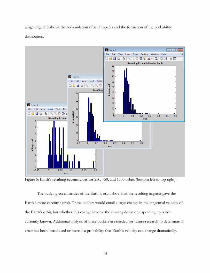
range. Figure 5 shows the accumulation of said impacts and the formation of the probability
distribution.
Figure 5: Earth’s resulting eccentricities for 250, 750, and 1500 orbits (bottom left to top right). The outlying eccentricities of the Earth’s orbit show that the resulting impacts gave the
Earth a more eccentric orbit. These outliers would entail a large change in the tangential velocity of
the Earth’s orbit, but whether this change involve the slowing down or a speeding up is not
currently known. Additional analysis of these outliers are needed for future research to determine if
error has been introduced or there is a probability that Earth’s velocity can change dramatically.
16
Results from the Runge-Kutta method are inconclusive, but do show a very different three-
body interaction that will be discussed more in 4.2 Error Analysis. The main difficulty that results
from the Runge-Kutta method is the chaotic orbits of the Earth and impactor as they enter into the
Earth’s Hill Sphere. The Hill Sphere is a region surrounding a planet in which its gravitational pull is
stronger than that of the Sun’s with a given proximity. The Earth’s Hill Sphere is located 0.01 AU
from the center or 9.96 × 10⁻³AU from the Earth’s surface.
4.2 Error Analysis
The error analysis within the Euler-Cromer method was to determine if a change in mass
affected the given eccentricities of Earth’s new orbit. A smaller mass was chosen and compared to
that of Mars. Previous giant impact research would approximate the needed mass of the impactor
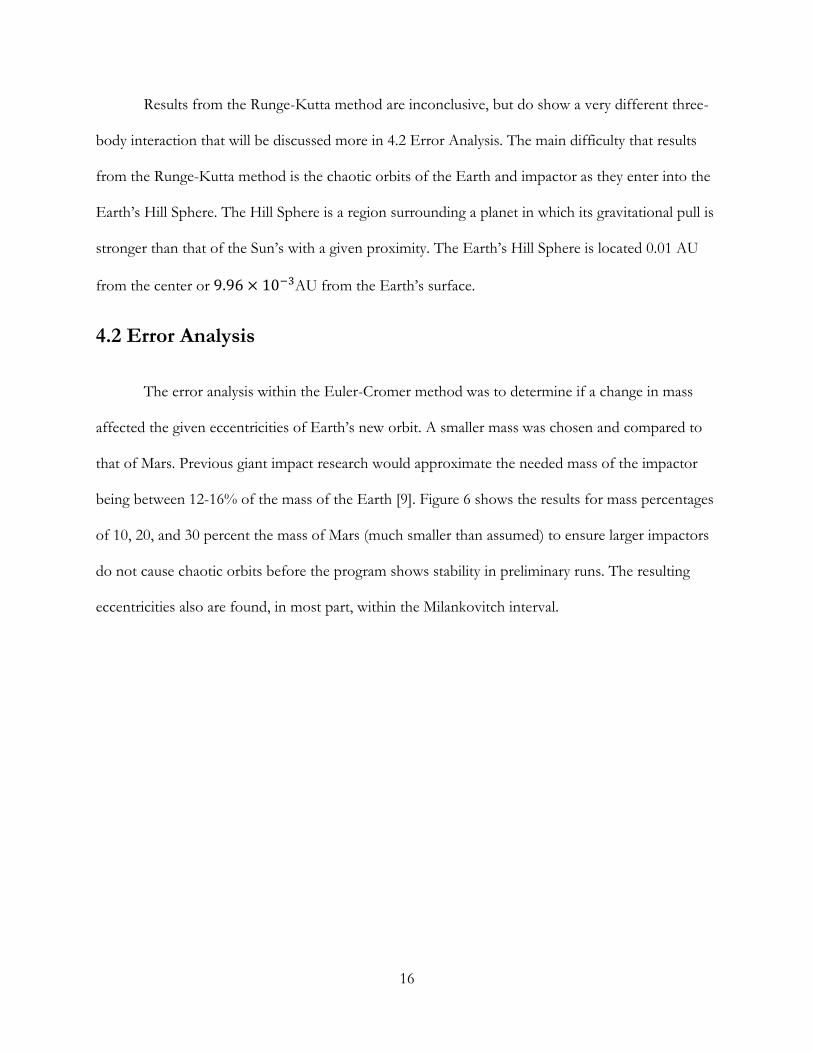
being between 12-16% of the mass of the Earth [9]. Figure 6 shows the results for mass percentages
of 10, 20, and 30 percent the mass of Mars (much smaller than assumed) to ensure larger impactors
do not cause chaotic orbits before the program shows stability in preliminary runs. The resulting
eccentricities also are found, in most part, within the Milankovitch interval.
17
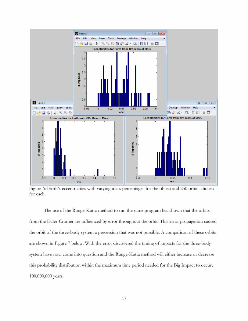
Figure 6: Earth’s eccentricities with varying mass percentages for the object and 250 orbits chosen for each. The use of the Runge-Kutta method to run the same program has shown that the orbits
from the Euler-Cromer are influenced by error throughout the orbit. This error propagation caused
the orbit of the three-body system a precession that was not possible. A comparison of these orbits
are shown in Figure 7 below. With the error discovered the timing of impacts for the three-body
system have now come into question and the Runge-Kutta method will either increase or decrease
this probability distribution within the maximum time period needed for the Big Impact to occur;
100,000,000 years.
18
Figure 7: Orbit Comparison between Euler-Cromer and Runge-Kutta methods. Top left and right images show how much the system precesses with ~50 years, time interval being .02 years, in the Euler-Cromer method. The Runge-Kutta method, bottom image, only shows slight variations in planet positions and no precession within the same interval.
During initial tests for the Runge-Kutta Method, it was realized that the time steps may be
too large to determine proximity within the Earth’s Hill’s Sphere. With reference to Figure 3: Euler
vs. Runge-Kutta [8] in chapter 2, the final values are too far apart to account for gravitational effects
on near collisions and too far apart to determine impact in crossing paths. The default time step of
.02 years was reduced to .002 years as Earth-to-Impactor distance was found to be less than the
current time step distance. This adjustment was not made for the Euler-Cromer method and is
another example of error found within the program and corrected within the new code.
19
Future analysis would involve the selection of one impact and adjust the time step to
reproduce the same resulting eccentricity for the Earth. A difference in eccentricities will show the
error involved when adjusting the time step for the given orbit. The Runge-Kutta method is more
accurate than Euler-Cromer by the fact that the orbits themselves do not involve precession without
the inclusion of larger orbiting bodies, such as Jupiter or Saturn.
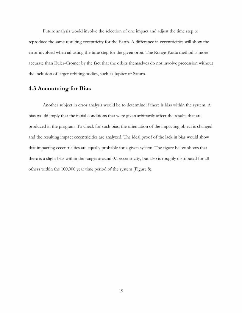
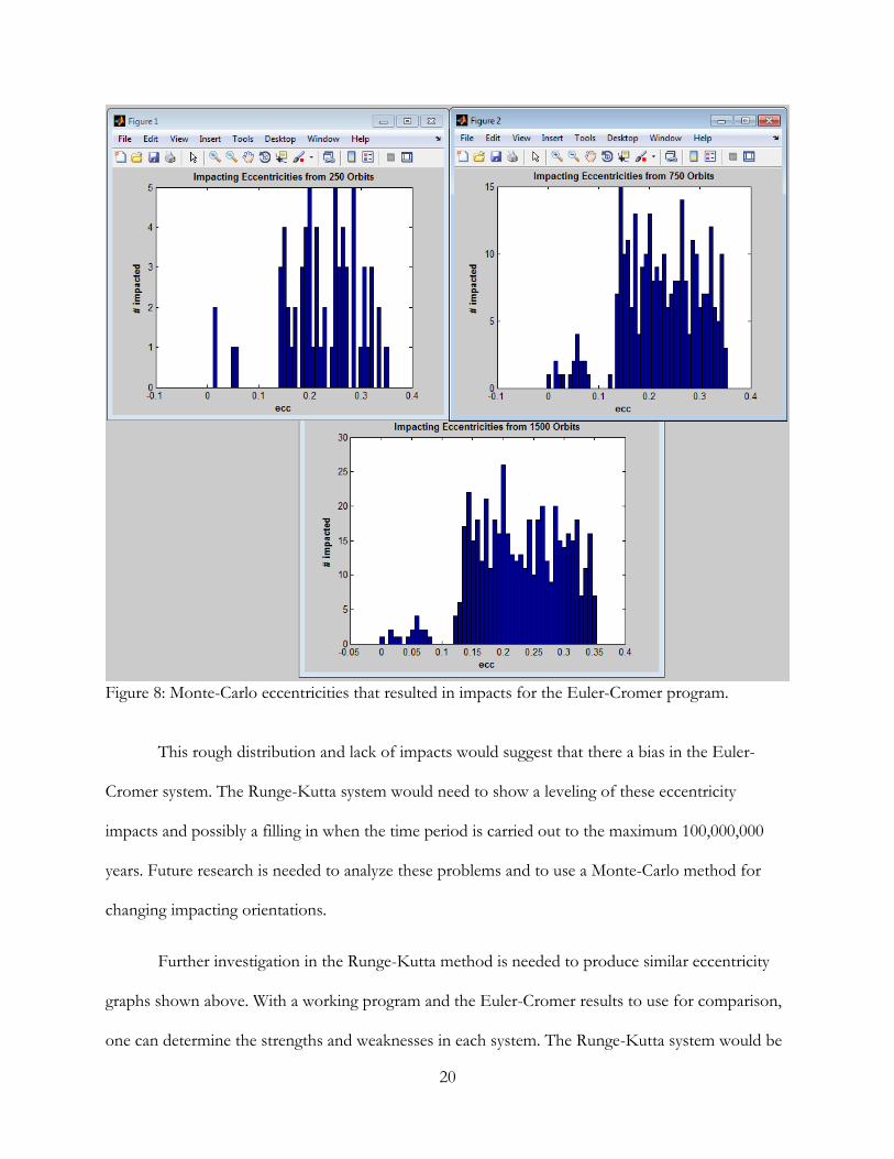
4.3 Accounting for Bias
Another subject in error analysis would be to determine if there is bias within the system. A
bias would imply that the initial conditions that were given arbitrarily affect the results that are
produced in the program. To check for such bias, the orientation of the impacting object is changed
and the resulting impact eccentricities are analyzed. The ideal proof of the lack in bias would show
that impacting eccentricities are equally probable for a given system. The figure below shows that
there is a slight bias within the ranges around 0.1 eccentricity, but also is roughly distributed for all
others within the 100,000 year time period of the system (Figure 8).
20
Figure 8: Monte-Carlo eccentricities that resulted in impacts for the Euler-Cromer program. This rough distribution and lack of impacts would suggest that there a bias in the Euler-
Cromer system. The Runge-Kutta system would need to show a leveling of these eccentricity
impacts and possibly a filling in when the time period is carried out to the maximum 100,000,000
years. Future research is needed to analyze these problems and to use a Monte-Carlo method for
changing impacting orientations.
Further investigation in the Runge-Kutta method is needed to produce similar eccentricity
graphs shown above. With a working program and the Euler-Cromer results to use for comparison,
one can determine the strengths and weaknesses in each system. The Runge-Kutta system would be
21
able to account for gravitational effects in proximity instances, but will need troubleshooting to
understand why a large number of orbits appear to become chaotic in time.
Chapter 5
Conclusion
5.1 Interpretation
It has been shown that the programming method of Euler-Cromer was a good start to
recreate a colliding system with just the Earth, Sun, and impactor being represented. In comparison
to the Runge-Kutta method, there is a large error propagation that causes the orbits to precess in the
Euler-Cromer method. As explained in chapter 1, the primary influence to Earth’s precession is due
to Jupiter and Saturn. A reduction in the time step for the Euler-Cromer method would minimize
this precession, but would sacrifice the processing time for said program. The default time step is
roughly one week out of the yearlong orbit of Earth.
The chaotic orbits in the Runge-Kutta method may stem from the total energy in the system.
As both planets come within proximity of each other numerous times, one of them exhibits a
constant loss of energy. This energy loss produces an inward spiral with increased velocity for the
planet until it enters close proximity to the Sun and subsequently is hurtled out into space. The
outlying planet does not appear to be greatly affected to this occurrence and continues in an
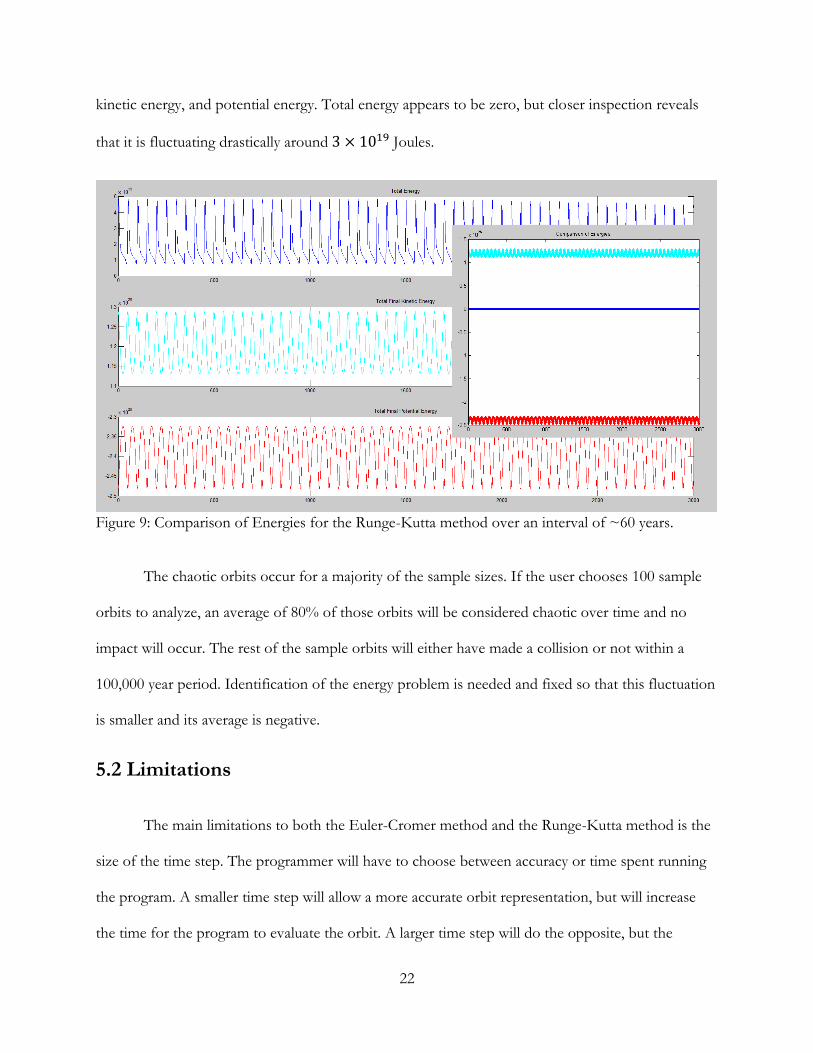
eccentric orbit around the Sun. Figure 9 below shows a comparison of the systems total energy,
22
kinetic energy, and potential energy. Total energy appears to be zero, but closer inspection reveals
that it is fluctuating drastically around 3 × 10¹⁹ Joules.
Figure 9: Comparison of Energies for the Runge-Kutta method over an interval of ~60 years. The chaotic orbits occur for a majority of the sample sizes. If the user chooses 100 sample
orbits to analyze, an average of 80% of those orbits will be considered chaotic over time and no
impact will occur. The rest of the sample orbits will either have made a collision or not within a
100,000 year period. Identification of the energy problem is needed and fixed so that this fluctuation
is smaller and its average is negative.
5.2 Limitations
The main limitations to both the Euler-Cromer method and the Runge-Kutta method is the
size of the time step. The programmer will have to choose between accuracy or time spent running
the program. A smaller time step will allow a more accurate orbit representation, but will increase
the time for the program to evaluate the orbit. A larger time step will do the opposite, but the
23
program itself may be manipulated in a way so that large steps out of collision proximity can be
reduced as the planets converge.
The program is written so that the positions and velocities of the three-body system is not
saved for every iteration, but is circular in assignment of each of the values. There are two variable
that are cycled; the current value and new value (e.g. 𝑥𝑒𝑎𝑟𝑡ℎ, 𝑥𝑒𝑎𝑟𝑡ℎ,𝑓𝑖𝑛𝑎𝑙; 𝑣𝑥,𝑒𝑎𝑟𝑡ℎ, 𝑣𝑥,𝑒𝑎𝑟𝑡ℎ,𝑓𝑖𝑛𝑎𝑙). As
the new value is evaluated in an iteration, at the end of the iteration this new value is assigned to the
name of the old value and a new iteration begins. The limitation for this method is the inability for
the user to view the scenario during the entire course of time. Though a graphing option has been
added to the program while it calculates the orbit, the processing time is increased drastically.
I would conclude that the program needs further investigation into the energy of the
systems, the eventual addition of the other planets within our solar system, and an increase in
processing capabilities. Many of the equations used within the current program are not simplified or
reduced for the intent of readability and organization. This will also limit processing capability, but
can be altered when the error propagations are reduced and analyzed.
5.3 Future Research
The goal of this research was to replicate the scenario of the Giant Impact Theory with
additional analysis of the resulting eccentric orbits that the Earth would take as a consequence of an
impact. With analysis, the research would show the probability that the Earth maintains a stable
orbit in the habitable zone of our solar system and imitates the Milankovitch cycles. This research
has capability to expand on this analysis by changing the initial conditions presented (e.g. impactors
orientation, Earth’s eccentric orbit, orbital tilt).
24
It would be very useful to incorporate a multi-processing system into the programming code
in which more than one central processing unit (CPU) is used to evaluate orbits. This would reduce
the processing time greatly by the number of orbit scenarios allotted to each CPU. The Physics
Department at Brigham Young University-Idaho is currently running a multi-processing system. The
current programming code for this research project would only need to be converted to C++
language for it to run on these CPU’s.
The next step for this research project would be to fix and analyze the error propagations
and energy fluctuations described in chapter 4. Without corrections to these orbital problems,
analysis of resulting eccentricities would be meaningless. Other alterations to the programming code
are encouraged and can lead to greater efficiency for the calculations of planetary orbit.
25
Bibliography
[1] S. Brush, “A History of Modern Selenogony: Theoretical Origins of the Moon, from Capture to
Crash 1955-1984,” University of Maryland, 1988.
[2] A. Cameron, “The Origin of the Moon and the Single Impact Hypothesis V,” Icarus 126-127,
1997.
[3] R. Canup, “Accretion of the Moon from an Impact-Generated Disk,” Icarus 119, 427-446, 1996.
[4] J. Hays et al., “Variations in the Earth’s Orbit: Pacemaker of the Ice Ages,” Science, Vol. 194 pp.
1121-1132, 1976.
[5] Taosi Astronomical Observatory, “Alternative Method for Precise Biao, Gnomon, Usage for
Determining the Location and Timing of the Sun’s Azimuthal Bearing and Elevation Angle,”
Phisical Psience [Image], 2014.
[6] R. Kopparapu, “A revised estimate of the occurrence rate of terrestrial planets in the habitable
zones around kepler m-dwarfs,” The Astrophysical Journal Letters 767(1), 2013.
[7] N. Giordano and H. Nakanishi, “Computational Physics, 2nd ed,” Pearson Education, Inc. pp.
94-118, 2006.
[8] W. Press et al., “Numerical Recipes: The Art of Scientific Computing,” Cambridge University
Press [Image], 1990.
[9] D. Stevenson, “Origin of the Moon—The Collision Hypothesis,” Annual Review of Earth and
Planetary Sciences 271-312, Annual Reviews Inc, 1987.
26
Appendix
MATLAB Code
% Orbital Consequences from the Giant Impact Hypothesis
% The purpose of this program is to recreate Earth's solar system prior to % the Giant Impact Hypothesis. The Giant Impact Hypothesis is a theory that % proposes the Moon's origin being another planet-like object within the % same distance as the Earth's orbit. Overtime the two planets collided and % the Earth-Moon system was the result. This is the Main file for the % program and the following are other function files related to running % this program properly: % impact_research.m (MAIN) % setup_variables.m % initial_impactor.m % montecarlo_eccentricities.m % euler_cromer_impact.m % impact.m % runge_kutta_impact.m % runge_impact.m
clear, close all; %////////////////////////////////////////////////////////////////////////% % Set constants and variables G = 1.985*10^(-29); %Gravitational constant, AU^3/(kg*yr^2) M = 1.989*10^30; %mass of the Sun, kg e = 0.0; %initial eccentricity a = 1; %semimajor-axis of Earth, AU r = a*(1 - e^2)/(1 + e); %Earth distance with initial angle, AU v = 2*pi*(a/r)*sqrt(((2*a)/r - 1)); %Earth velocity (vis viva), AU/yr Me = 5.97*10^24 + 7.36*10^22; %mass of the Earth-Moon system, kg P = sqrt((4*pi^2*a^3)/(G*(M + Me)));%period of the Earth, yr RH = .01; %Earth's Hill's Sphere, AU
% Set up time interval tf = 100000; %years, max is 1*10^8
% Choose a time step in years dt = 0.02; % dt = 0.0191130351; %.02yr = 7.305day
%////////////////////////////////////////////////////////////////////////% % Ask whether the program is a continuation from a previous program that % was paused before it's last iteration. program = 2; %input validator display... ('Program requires masspercent, MO, Me, EO, ecc, imp, n, graph, i') while (program == 2)
27
program = input('Is there a program you wish to continue(Y=1,N=0)? '); if program == 1 || program == 0 %input validation else program = 2; end end
%////////////////////////////////////////////////////////////////////////% % Setup impactor's variables dependent on whether it is a continuation or % not. if program == 0 % Function to setup variables and arrays [EO, MO, Me, ecc, imp, ImpEcc, graph] = setup_variables(Me); n = 1; %initial value for loop i = 0; %initial value for impacts elseif program == 1 file = input('Workspace file name (e.g. file_name.mat): ', 's'); load(file); end
%\\\\\\\\\\\\\\\\\\\\\\\\\\\\\\\\\\\\\\\\\\\\\\\\\\\\\\\\\\\\\\\\\\\\\\\\% % Loop through eccentricities for impactor while n <= length(EO) eO = EO(n); %designate object eccentricity
% Function for impactor's initial conditions [rO, vO] = initial_impactor(MO, M, G, eO);
gr = sqrt((graph - eO)^2)/eO; %find graph average difference if gr < .05 %turn on graph for ecc within 5% graph = 1; end
% Function for impact and orbit [ECC, impact] = runge_kutta_impact(G, M, ... Me, MO, tf, dt, RH, a, e, v, rO, vO, graph);
if graph == 1 graph = 0; %turn off graph end
if impact > 0 %if impact occurs ecc(n) = ECC; %set Earth resulting eccentricity imp(n) = impact; %set impacting time ImpEcc(n) = eO; %save impacting eccentricity i = i + 1; %iterate number of impacts %display(i); end n = n + 1; %iterate loop %disp(n); end
%////////////////////////////////////////////////////////////////////////% % Histogram of Earth's resulting eccentricities and the impactors' % eccentricities that caused them.
28
if i ~= 0 figure(2); subplot(1,2,1); E1 = transpose(nonzeros(ecc)); %setup Earth eccentricity array intervals = linspace(0, max(E1), 35);%setup intervals for histogram hist(E1, intervals); title('Eccentricity of Earth', 'Fontweight', 'bold'); xlabel('ecc', 'Fontweight', 'bold'); ylabel('# of orbits', 'Fontweight', 'bold');
subplot(1,2,2); E2 = transpose(nonzeros(ImpEcc)); %setup Impactor eccentricity array intervals = linspace(0, max(E2), 35);%setup intervals for histogram hist(E2, intervals); title('Eccentricity of Earth', 'Fontweight', 'bold'); xlabel('ecc', 'Fontweight', 'bold'); ylabel('# of orbits', 'Fontweight', 'bold'); end
% By Anthony Hales ([email protected])
% Impacting Object's Initial Conditions
% This function file is related to the main program impact_research.m and % its use is to designate the impactor's initial conditions. The file % impact_research.m will call this function.
function [rO, vO] = initial_impactor(MO, M, G, eO)
aO = 1; %semi-major axis, AU rO = aO*(1 - eO^2)/(1 + eO); %distance from sun, AU PO = sqrt((4*pi^2*aO^3)/(G*(M + MO))); %period of orbit, yr vO = (2*pi*aO*sqrt(((2*aO)/rO - 1)))/PO; %tangential speed, AU/yr
end
% Object's Constants and Variables
% This function file is related to the main program impact_research.m and % is to setup user variables and arrays used for the impactor and the % graphing option for the program. The file impact_research.m will call % this function.
function [EO,MO,Me,ecc,imp,ImpEcc,graph] = setup_variables(Me)
masspercent = 0; %mass pre-allocation
while (masspercent == 0) masspercent = input... ('What mass percentage is the impactor(0 < m% < 1)? '); end
MO = masspercent*Me; %percentage of Earth-Moon mass
29
Me = Me - MO; %adjust Earth-Moon's mass
%////////////////////////////////////////////////////////////////////////% % Random eccentricities will be chosen from user input disp('Eccentricity range: .001 < e < .35') num = input... ('How many sample eccentricities would you like? '); while isempty(num) || num < 1 %input validation num = input('How many sample eccentricities would you like? '); end
%////////////////////////////////////////////////////////////////////////% % Function for eccentricity interval [EO] = montecarlo_eccentricities(num);
ecc = zeros(1,num); %eccentricity pre-allocation imp = zeros(1,num); %impact pre-allocation ImpEcc = zeros(1,num); %impact ecc pre-allocation disp('If a graph is not wanted, input 0.'); graph = input... ('What eccentricity would you like to graph(.001 < e < .35)? '); if isempty(graph) %graph no response pre-allocation graph = EO(1); %graphing first eccentricity elseif graph == 0 graph = .9; %number indicates impossible graph end
end
% Monte-Carlo Setup for Object Eccentricities
% This function file is related to the main program impact_research.m and % will allocate for a set number of orbits and then designate random % eccentricities for that orbit. The file setup_variables.m will call this % function.
function [eO] = montecarlo_eccentricities(num)
eccO = zeros(1,num); %pre-allocate orbit array
for n=1:num rng('shuffle'); %designate random num generator eccO(n) = (.35 - .001)*rand(1) + .001; %maintain interval, .001 to .35 end
eO = eccO(1:num); %rename orbit array
end
% Euler-Cromer Method for Orbit
% This function file is related to the main program impact_research.m and % its use is to evaluate the orbits in a planetary system within the given
30
% time step. It also has the capability of graphing according to the user % input and determine proximity of colliding impact. The file % impact_research.m will call this function.
function [ECC, Imp] = euler_cromer_impact(G, M, ... Me, MO, tf, dt, RH, a, e, v, rO, vO, graph)
% Initial Earth conditions for orbit xe = a*(1 - e^2)/(1 + e); %AU ye = 0; %AU vxe = 0; %AU/yr vye = v; %Au/yr % Initial Sun conditions for orbit xs = 0; %AU ys = 0; %AU vxs = 0; %AU/yr vys = -v*(Me/M); %AU/yr % Initial impactor conditions for orbit xO = 0; %AU yO = -rO; %AU vxO = vO; %AU/yr vyO = 0; %AU/yr
%////////////////////////////////////////////////////////////////////////% i = 0; %impact indicator t = 0; %initialize time
% Turn on graphing capability if graph == 1 hold on; end
%////////////////////////////////////////////////////////////////////////% % Loop through alloted time interval while t < tf res = (((xe-xs)^2) + ((ye-ys)^2))^(1/2); %distance Earth to Sun rOs = (((xO-xs)^2) + ((yO-ys)^2))^(1/2); %distance impactor to Sun rOe = (((xO-xe)^2) + ((yO-ye)^2))^(1/2); %distance impactor to Earth
% Determine if object reaches escape velocity v = ((vxO^2) + (vyO^2))^(1/2); %magnitude AU/yr vesc = (2*G*M/rOs)^(1/2); %escape velocity if v >= vesc %end loop of orbit ECC = 0; Imp = 0; break; end
% Impactor in range of Earth's Hill Sphere if rOe < RH % Function to reduce time step and record possible impact [xe, ye, xO, yO, xs, ys, vxe, vye, vxO, vyO, vxs, vys, ecc, ... imp] = euler_impact(G, M, Me, MO, tf, dt, t, vxe, vye, vxs, ... vys, vxO, vyO, xe, ye, xs, ys, xO, yO, RH);
31
%////////////////////////////////////////////////////////////////% % If Earth's eccentricity has a value then record the time of % impact and rename the eccentricity variable else restore time % step and continue loop. if ecc > 0 Imp = imp; i = 1; ECC = ecc; break; else t = imp; dt = .02; end %////////////////////////////////////////////////////////////////% end
% Earth's velocity vxef = vxe - ((G*M*(xe - xs))/(res^3))*dt... - ((G*MO*(xe - xO))/(rOe^3))*dt; vyef = vye - ((G*M*(ye - ys))/(res^3))*dt... - ((G*MO*(ye - yO))/(rOe^3))*dt;
% Impactor's velocity vxOf = vxO - ((G*M*(xO - xs))/(rOs^3))*dt... - ((G*Me*(xO - xe))/(rOe^3))*dt; vyOf = vyO - ((G*M*(yO - ys))/(rOs^3))*dt... - ((G*Me*(yO - ye))/(rOe^3))*dt;
% Sun's velocity vxsf = vxs - ((G*Me*(xs - xe))/(res^3))*dt; vysf = vys - ((G*Me*(ys - ye))/(res^3))*dt;
% Earth's position xef = xe + vxef*dt; yef = ye + vyef*dt;
%Sun's position xsf = xs + vxsf*dt; ysf = ys + vysf*dt;
%Impactor's position xOf = xO + vxOf*dt; yOf = yO + vyOf*dt;
t = t + dt; %time step
%////////////////////////////////////////////////////////////////////% % Allocate future value to current value xe = xef; ye = yef; vxe = vxef; vye = vyef; xs = xsf; ys = ysf; vxs = vxsf;
32
vys = vysf; xO = xOf; yO = yOf; vxO = vxOf; vyO = vyOf;
%////////////////////////////////////////////////////////////////////% % Orbital graphing if graph == 1 plot(xe, ye, '.w', 'MarkerSize', 4); plot(xs, ys, 'oy', 'MarkerSize', 4'); plot(xO, yO, '.g', 'MarkerSize', 4); set(gca, 'color', [0.1 0.1 0.1]); axis square; axis([-2 2 -2 2]); title('Earth orbiting the Sun', 'Fontweight', 'bold'); xlabel('x (AU)', 'Fontweight', 'bold'); ylabel('y (AU)', 'Fontweight', 'bold'); pause(.01); end
%////////////////////////////////////////////////////////////////////% end
% Turn off graphing capability if graph == 1 hold off; end
% Current impactor made no impact if i == 0 ECC = 0; Imp = 0; end
end
%Impact Analysis
% This function file is related to the main program impact_research.m and % its use is to determine if an impact has occurred and determine the new % eccentricity for the Earth. The file euler_cromer_impact.m will call this % function.
function [Xe, Ye, XO, YO, Xs, Ys, Vxe, Vye, VxO, VyO, Vxs, Vys, ecc, ... imp] = euler_impact(G, M, Me, MO, tf, dt, t, vxe, vye, vxs, vys, ... vxO, vyO, xe, ye, xs, ys, xO, yO, RH)
dt = dt*.001; %reduce time-step RE = .00004; %radius of Earth, AU rOe = (((xO-xe)^2) + ((yO-ye)^2))^(1/2); %distance impactor to Earth r = rOe; %distance indicator disp('Object is near');
33
%////////////////////////////////////////////////////////////////////////% % Loop through alloted time interval while (t < tf && rOe < RH && r <= rOe) res = (((xe-xs)^2) + ((ye-ys)^2))^(1/2); %distance Earth to Sun rOs = (((xO-xs)^2) + ((yO-ys)^2))^(1/2); %distance impactor to Sun rOe = (((xO-xe)^2) + ((yO-ye)^2))^(1/2); %distance impactor to Earth
% Impactor hits within the radius of Earth if rOe < RE Vxe = (Me*vxe + MO*vxO)/(Me + MO); %new x-velocity Vye = (Me*vye + MO*vyO)/(Me + MO); %new y-velocity VxO = 0; %null object's velocity VyO = 0; %null object's velocity %Me = Me + MO; %adjust to Earth-Moon mass MO = 0; %null object's mass imp = t; %time of impact, yr tanv = (vxe^2 + vye^2)^(1/2); %tangential velocity ecc = (1 + (((tanv^4)*(res^2)) - (2*G*M*res*(tanv^2)))... /((G^2)*(M^2)))^(1/2); %new eccentricity
% Reassign positions Xe = xe; Ye = ye; XO = xO; YO = yO; Xs = xs; Ys = ys; Vxs = vxs; Vys = vys; break; %end loop end
%////////////////////////////////////////////////////////////////////% % Earth's velocity vxef = vxe - ((G*M*(xe - xs))/(res^3))*dt... - ((G*MO*(xe - xO))/(rOe^3))*dt; vyef = vye - ((G*M*(ye - ys))/(res^3))*dt... - ((G*MO*(ye - yO))/(rOe^3))*dt;
% Impactor's velocity vxOf = vxO - ((G*M*(xO - xs))/(rOs^3))*dt... - ((G*Me*(xO - xe))/(rOe^3))*dt; vyOf = vyO - ((G*M*(yO - ys))/(rOs^3))*dt... - ((G*Me*(yO - ye))/(rOe^3))*dt;
% Sun's velocity vxsf = vxs - ((G*Me*(xs - xe))/(res^3))*dt; vysf = vys - ((G*Me*(ys - ye))/(res^3))*dt;
% Earth's position xef = xe + vxef*dt; yef = ye + vyef*dt;
%Sun's position xsf = xs + vxsf*dt;
34
ysf = ys + vysf*dt;
%Impactor's position xOf = xO + vxOf*dt; yOf = yO + vyOf*dt;
t = t + dt; %time step
%////////////////////////////////////////////////////////////////////% % Allocate future value to current value xe = xef; ye = yef; vxe = vxef; vye = vyef; xs = xsf; ys = ysf; vxs = vxsf; vys = vysf; xO = xOf; yO = yOf; vxO = vxOf; vyO = vyOf; %////////////////////////////////////////////////////////////////////%
r = (((xO-xe)^2) + ((yO-ye)^2))^(1/2); %distance indicator end
%////////////////////////////////////////////////////////////////////////% % Current impactor made no impact, reallocate variables if MO > 0 Xe = xe; Ye = ye; XO = xO; YO = yO; Xs = xs; Ys = ys; Vxe = vxe; Vye = vye; VxO = vxO; VyO = vyO; Vxs = vxs; Vys = vys; imp = t; ecc = 0; end
end
% Runge-Kutta Method for Orbit
% This function file is related to the main program impact_research.m and % its use is to evaluate the orbits in a planetary system within the given % time step. It also has the capability of graphing according to the user % input and determine proximity of colliding impact. The file
35
% impact_research.m will call this function.
function [ECC, Imp] = runge_kutta_impact(G, M, ... Me, MO, tf, dt, RH, a, e, v, rO, vO, graph)
% Initial Earth conditions for orbit xe = a*(1 - e^2)/(1 + e); %AU ye = 0; %AU vxe = 0; %AU/yr vye = v; %AU/yr % Initial Sun conditions for orbit Srad = 0.004651; %radius of Sun, AU xs = 0; %AU ys = 0; %AU vxs = -vO*(MO/M); %AU/yr vys = -v*(Me/M); %AU/yr % Initial impactor conditions for orbit xO = 0; %AU yO = -rO; %AU vxO = vO; %AU/yr vyO = 0; %AU/yr
% Initialize indicators i = 0; %impact indicator t = 0; %initialize time approaching = 0; %proximity indicator delta = 0.002; %Hill's Sphere time step n=1; %////////////////////////////////////////////////////////////////////////% % Loop through allotted time interval while t < tf
%**********Troubleshooting***************%
% Turn on graph at a given time. % if t > 1.80317307e+04 % graph = 1; % end %****************************************%
res = (((xe-xs)^2) + ((ye-ys)^2))^(1/2); %distance Earth to Sun rOs = (((xO-xs)^2) + ((yO-ys)^2))^(1/2); %distance impactor to Sun rOe = (((xO-xe)^2) + ((yO-ye)^2))^(1/2); %distance impactor to Earth
% Impactor or Earth spiraled into the Sun if rOs <= Srad || res <= Srad display('Sun Impact') break; end
%////////////////////////////////////////////////////////////////////% % Impactor in range of Earth's Hill Sphere if rOe < RH chart = graph; %save previous graph value graph = 1; %turn on graph
36
% Function for impactor entering into Earth's Hill's Sphere. The % Hill's Sphere is where the gravity of the Earth is stronger on an % object than the Sun's gravity. [xe, ye, xO, yO, xs, ys, vxe, vye, vxO, vyO, vxs, vys, ecc, ... imp] = runge_impact(G, M, Me, MO, tf, dt, t, vxe, vye, vxs, ... vys, vxO, vyO, xe, ye, xs, ys, xO, yO, RH, graph);
graph = chart; %return previous value if ecc > 0 %indicates impact value Imp = imp; %time of impact i = 1; %impact iteration ECC = ecc; %Earth's new eccentricity break; else t = imp; %continue time dt = .0002; %restore time step end end
%////////////////////////////////////////////////////////////////////% % Determine if object reaches escape velocity v = ((vxO^2) + (vyO^2))^(1/2); %magnitude AU/yr vesc = (2*G*M/rOs)^(1/2); %escape velocity if v >= vesc && rOe > 1 %end loop of orbit disp('Gone') display(v) format long; %15 significant figures display(t); format; %default significant fig. break; end
%////////////////////////////////////////////////////////////////////% % Runge Kutta 4th Order defined by the following: x(t+dt) = x(t) + % 1/6[f(x1',t1') + 2f(x2',t2') + 2f(x3',t3') + f(x4',t4')]dt, where % x1'=x(t), x2'=x(t)+1/2f(x1',t1')dt, x3'=x(t)+1/2f(x2',t2')dt, x4'= % x(t)+f(x3',t3')dt, t1'=t, t2'=t+1/2dt, t3'=t+1/2dt, t4'=t+dt.
% f(v1'): velocity of Earth, Impactor, and Sun vxe1 = -((G*M*(xe - xs))/(res^3))*dt - ((G*MO*(xe - xO))/(rOe^3))*dt; vye1 = -((G*M*(ye - ys))/(res^3))*dt - ((G*MO*(ye - yO))/(rOe^3))*dt; vxO1 = -((G*M*(xO - xs))/(rOs^3))*dt - ((G*Me*(xO - xe))/(rOe^3))*dt; vyO1 = -((G*M*(yO - ys))/(rOs^3))*dt - ((G*Me*(yO - ye))/(rOe^3))*dt; vxs1 = -((G*MO*(xs - xO))/(rOs^3))*dt - ((G*Me*(xs - xe))/(res^3))*dt; vys1 = -((G*MO*(ys - yO))/(rOs^3))*dt - ((G*Me*(ys - ye))/(res^3))*dt;
% f(x1'): position of Earth, Impactor, and Sun xe1 = vxe*dt; ye1 = vye*dt; xO1 = vxO*dt; yO1 = vyO*dt; xs1 = vxs*dt; ys1 = vys*dt;
% f(v2'): velocity of Earth, Impactor, and Sun vxe2 = -((G*M*(xe + xe1/2 - (xs + xs1/2)))/(((xe + xe1/2 - ...
37
(xs + xs1/2))^2) + ((ye + ye1/2 - (ys + ys1/2))^2))^(3/2))*dt... - ((G*MO*(xe + xe1/2 - (xO + xO1/2)))/(((xe + xe1/2 - ... (xO + xO1/2))^2) + ((ye + ye1/2 - (yO + yO1/2))^2))^(3/2))*dt;
vye2 = -((G*M*(ye + ye1/2 - (ys + ys1/2)))/(((xe + xe1/2 - ... (xs + xs1/2))^2) + ((ye + ye1/2 - (ys + ys1/2))^2))^(3/2))*dt... - ((G*MO*(ye + ye1/2 - (yO + yO1/2)))/(((xe + xe1/2 - ... (xO + xO1/2))^2) + ((ye + ye1/2 - (yO + yO1/2))^2))^(3/2))*dt;
vxO2 = -((G*M*(xO + xO1/2 - (xs + xs1/2)))/(((xO + xO1/2 - ... (xs + xs1/2))^2) + ((yO + yO1/2 - (ys + ys1/2))^2))^(3/2))*dt... - ((G*Me*(xO + xO1/2 - (xe + xe1/2)))/(((xO + xO1/2 - ... (xe + xe1/2))^2) + ((yO + yO1/2 -(ye + ye1/2))^2))^(3/2))*dt;
vyO2 = -((G*M*(yO + yO1/2 - (ys + ys1/2)))/(((xO + xO1/2 - ... (xs + xs1/2))^2) + ((yO + yO1/2 - (ys + ys1/2))^2))^(3/2))*dt... - ((G*Me*(yO + yO1/2 - (ye + ye1/2)))/(((xO + xO1/2 - ... (xe + xe1/2))^2) + ((yO + yO1/2 -(ye + ye1/2))^2))^(3/2))*dt;
vxs2 = -((G*Me*(xs + xs1/2 - (xe + xe1/2)))/(((xs + xs1/2 - ... (xe + xe1/2))^2) + ((ys + ys1/2 - (ye + ye1/2))^2))^(3/2))*dt... - ((G*MO*(xs + xs1/2 - (xO + xO1/2)))/(((xs + xs1/2 - ... (xO + xO1/2))^2) + ((ys + ys1/2 - (yO + yO1/2))^2))^(3/2))*dt;
vys2 = -((G*Me*(ys + ys1/2 - (ye + ye1/2)))/(((xs + xs1/2 - ... (xe + xe1/2))^2) + ((ys + ys1/2 - (ye + ye1/2))^2))^(3/2))*dt... - ((G*MO*(ys + ys1/2 - (yO + yO1/2)))/(((xs + xs1/2 - ... (xO + xO1/2))^2) + ((ys + ys1/2 - (yO + yO1/2))^2))^(3/2))*dt;
% f(x2'): position of Earth, Impactor, and Sun xe2 = (vxe + vxe1/2)*dt; ye2 = (vye + vye1/2)*dt; xO2 = (vxO + vxO1/2)*dt; yO2 = (vyO + vyO1/2)*dt; xs2 = (vxs + vxs1/2)*dt; ys2 = (vys + vys1/2)*dt;
% f(v3'): velocity of Earth, Impactor, and Sun vxe3 = -((G*M*(xe + xe2/2 - (xs + xs2/2)))/(((xe + xe2/2 - ... (xs + xs2/2))^2) + ((ye + ye2/2 - (ys + ys2/2))^2))^(3/2))*dt... - ((G*MO*(xe + xe2/2 - (xO + xO2/2)))/(((xe + xe2/2 - ... (xO + xO2/2))^2) + ((ye + ye2/2 - (yO + yO2/2))^2))^(3/2))*dt;
vye3 = -((G*M*(ye + ye2/2 - (ys + ys2/2)))/(((xe + xe2/2 - ... (xs + xs2/2))^2) + ((ye + ye2/2 - (ys + ys2/2))^2))^(3/2))*dt... - ((G*MO*(ye + ye2/2 - (yO + yO2/2)))/(((xe + xe2/2 - ... (xO + xO2/2))^2) + ((ye + ye2/2 - (yO + yO2/2))^2))^(3/2))*dt;
vxO3 = -((G*M*(xO + xO2/2 - (xs + xs2/2)))/(((xO + xO2/2 - ... (xs + xs2/2))^2) + ((yO + yO2/2 - (ys + ys2/2))^2))^(3/2))*dt... - ((G*Me*(xO + xO2/2 - (xe + xe2/2)))/(((xO + xO2/2 - ... (xe + xe2/2))^2) + ((yO + yO2/2 - (ye + ye2/2))^2))^(3/2))*dt;
vyO3 = -((G*M*(yO + yO2/2 - (ys + ys2/2)))/(((xO + xO2/2 - ... (xs + xs2/2))^2) + ((yO + yO2/2 - (ys + ys2/2))^2))^(3/2))*dt...
38
- ((G*Me*(yO + yO2/2 - (ye + ye2/2)))/(((xO + xO2/2 - ... (xe + xe2/2))^2) + ((yO + yO2/2 - (ye + ye2/2))^2))^(3/2))*dt;
vxs3 = -((G*Me*(xs + xs2/2 - (xe + xe2/2)))/(((xs + xs2/2 - ... (xe + xe2/2))^2) + ((ys + ys2/2 - (ye + ye2/2))^2))^(3/2))*dt... - ((G*MO*(xs + xs2/2 - (xO + xO2/2)))/(((xs + xs2/2 - ... (xO + xO2/2))^2) + ((ys + ys2/2 - (yO + yO2/2))^2))^(3/2))*dt;
vys3 = -((G*Me*(ys + ys2/2 - (ye + ye2/2)))/(((xs + xs2/2 - ... (xe + xe2/2))^2) + ((ys + ys2/2 - (ye + ye2/2))^2))^(3/2))*dt... - ((G*MO*(ys + ys2/2 - (yO + yO2/2)))/(((xs + xs2/2 - ... (xO + xO2/2))^2) + ((ys + ys2/2 - (yO + yO2/2))^2))^(3/2))*dt;
% f(x3'): position of Earth, Impactor, and Sun xe3 = (vxe + vxe2/2)*dt; ye3 = (vye + vye2/2)*dt; xO3 = (vxO + vxO2/2)*dt; yO3 = (vyO + vyO2/2)*dt; xs3 = (vxs + vxs2/2)*dt; ys3 = (vys + vys2/2)*dt;
% f(v4'): velocity of Earth, Impactor, and Sun vxe4 = -((G*M*(xe + xe3 - (xs + xs3)))/(((xe + xe3 - (xs + xs3))^2)... + ((ye + ye3 - (ys + ys3))^2))^(3/2))*dt - ... ((G*MO*(xe + xe3 - (xO + xO3)))/(((xe + xe3 - (xO + xO3))^2) + ... ((ye + ye3 - (yO + yO3))^2))^(3/2))*dt;
vye4 = -((G*M*(ye + ye3 - (ys + ys3)))/(((xe + xe3 - (xs + xs3))^2)... + ((ye + ye3 - (ys + ys3))^2))^(3/2))*dt - ... ((G*MO*(ye + ye3 - (yO + yO3)))/(((xe + xe3 - (xO + xO3))^2) + ... ((ye + ye3 - (yO + yO3))^2))^(3/2))*dt;
vxO4 = -((G*M*(xO + xO3 - (xs + xs3)))/(((xO + xO3 - (xs + xs3))^2)... + ((yO + yO3 - (ys + ys3))^2))^(3/2))*dt - ... ((G*Me*(xO + xO3 - (xe + xe3)))/(((xO + xO3 - (xe + xe3))^2) + ... ((yO + yO3 - (ye + ye3))^2))^(3/2))*dt;
vyO4 = -((G*M*(yO + yO3 - (ys + ys3)))/(((xO + xO3 - (xs + xs3))^2)... + ((yO + yO3 - (ys + ys3))^2))^(3/2))*dt - ... ((G*Me*(yO + yO3 - (ye + ye3)))/(((xO + xO3 - (xe + xe3))^2) + ... ((yO + yO3 - (ye + ye3))^2))^(3/2))*dt;
vxs4 = -((G*Me*(xs + xs3 - (xe + xe3)))/(((xs + xs3 - (xe + xe3))^2)... + ((ys + ys3 - (ye + ye3))^2))^(3/2))*dt - ... ((G*MO*(xs + xs3 - (xO + xO3)))/(((xs + xs3 - (xO + xO3))^2) + ... ((ys + ys3 - (yO + yO3))^2))^(3/2))*dt;
vys4 = -((G*Me*(ys + ys3 - (ye + ye3)))/(((xs + xs3 - (xe + xe3))^2)... + ((ys + ys3 - (ye + ye3))^2))^(3/2))*dt - ... ((G*MO*(ys + ys3 - (yO + yO3)))/(((xs + xs3 - (xO + xO3))^2) + ... ((ys + ys3 - (yO + yO3))^2))^(3/2))*dt;
% f(x4'): position of Earth, Impactor, and Sun xe4 = (vxe + vxe3)*dt; ye4 = (vye + vye3)*dt;
39
xO4 = (vxO + vxO3)*dt; yO4 = (vyO + vyO3)*dt; xs4 = (vxs + vxs3)*dt; ys4 = (vys + vys3)*dt;
% Earth's velocity vxef = vxe + (vxe1 + 2*vxe2 + 2*vxe3 + vxe4)/6; vyef = vye + (vye1 + 2*vye2 + 2*vye3 + vye4)/6;
% Impactor's velocity vxOf = vxO + (vxO1 + 2*vxO2 + 2*vxO3 + vxO4)/6; vyOf = vyO + (vyO1 + 2*vyO2 + 2*vyO3 + vyO4)/6;
% Sun's velocity vxsf = vxs + (vxs1 + 2*vxs2 + 2*vxs3 + vxs4)/6; vysf = vys + (vys1 + 2*vys2 + 2*vys3 + vys4)/6;
% Earth's position xef = xe + (xe1 + 2*xe2 + 2*xe3 + xe4)/6; yef = ye + (ye1 + 2*ye2 + 2*ye3 + ye4)/6;
% Impactor's position xOf = xO + (xO1 + 2*xO2 + 2*xO3 + xO4)/6; yOf = yO + (yO1 + 2*yO2 + 2*yO3 + yO4)/6;
% Sun's position xsf = xs + (xs1 + 2*xs2 + 2*xs3 + xs4)/6; ysf = ys + (ys1 + 2*ys2 + 2*ys3 + ys4)/6;
%////////////////////////////////////////////////////////////////////% % Determine if planets are approaching each other by comparing the size % of their time step between the initial position and final position to % the distance between each other. If an approach occurs, mark the time % step boundary and set time one step back in case a crossing path % occurred before the approaching distance was determined. Reset % positions and velocities as well as reduce time step to Hill's Sphere % distance.
if approaching == 0 % Time step distance of Earth's initial vs. final position rife = (((xef-xe)^2) + ((yef-ye)^2))^(1/2); % Time step distance of impactor's initial vs. final position rifO = (((xOf-xO)^2) + ((yOf-yO)^2))^(1/2); % Distance impactor to Earth rOe = (((xOf-xef)^2) + ((yOf-yef)^2))^(1/2);
% Planets are now in proximity from one to another if rOe <= rife || rOe <= rifO step = t + dt; %mark final time boundary t = t - dt; %reset one step back dt = delta; %Hill's Sphere time step % Reset position and velocity xef = xe; yef = ye; xOf = xO;
40
yOf = yO; xsf = xs; ysf = ys; vxef = vxe; vyef = vye; vxOf = vxO; vyOf = vyO; approaching = 1; %proximity alerted %disp('proximity alerted'); end % With proximity alerted, determine if time reached final boundary elseif approaching == 1 if t >= step approaching = 0; %proximity off dt = .02; %time step reset %disp('proximity off'); end end
resf = (((xef-xsf)^2) + ((yef-ysf)^2))^(1/2);%distance Earth to Sun rOsf = (((xOf-xsf)^2) + ((yOf-ysf)^2))^(1/2);%distance impactor to Sun rOef = (((xOf-xef)^2)+((yOf-yef)^2))^(1/2); %distance impactor to Earth
Energy(n) = -(G*M*Me)/res - (G*M*MO)/rOs - (G*Me*MO)/rOe + ... (G*M*Me)/resf + (G*M*MO)/rOsf + (G*Me*MO)/rOef + ... (Me*(vxe^2 + vye^2))/2 + (MO*(vxO^2 + vyO^2))/2 + ... (M*(vxs^2 + vys^2))/2 - (Me*(vxef^2 + vyef^2))/2 - ... (MO*(vxOf^2 + vyOf^2))/2 - (M*(vxsf^2 + vysf^2))/2;
KineticE(n) = (Me*(vxef^2 + vyef^2))/2 + (MO*(vxOf^2 + vyOf^2))/2 + ... (M*(vxsf^2 + vysf^2))/2;
PotentialE(n) = -(G*M*Me)/resf - (G*M*MO)/rOsf - (G*Me*MO)/rOef;
n=n+1;
if n == 30000 figure(3); subplot(1,3,1); plot(Energy, '.b'); title('Total Energy'); subplot(1,3,2); plot(KineticE, '.c'); title('Total Final Kinetic Energy'); subplot(1,3,3); plot(PotentialE, '.r'); title('Total Final Potential Energy'); figure(4); plot(1:n-1, Energy, '.b', 1:n-1, KineticE, '.c', 1:n-1, PotentialE,
'.r'); title('Comparison of Energies'); pause; end
%////////////////////////////////////////////////////////////////////%
41
t = t + dt; %time step
% Allocate future value to current value xe = xef; ye = yef; vxe = vxef; vye = vyef; xs = xsf; ys = ysf; vxs = vxsf; vys = vysf; xO = xOf; yO = yOf; vxO = vxOf; vyO = vyOf;
%////////////////////////////////////////////////////////////////////% % Orbital graphing if graph == 1 hold on; drawnow; plot(xe, ye, 'og', 'MarkerSize', 4); plot(xs, ys, 'oy', 'MarkerSize', 10'); plot(xO, yO, 'or', 'MarkerSize', 2); set(gca, 'color', [0.1 0.1 0.1]); axis square; axis([-2.5 2.5 -2.5 2.5]); title('Earth orbiting the Sun', 'Fontweight', 'bold'); xlabel('x (AU)', 'Fontweight', 'bold'); ylabel('y (AU)', 'Fontweight', 'bold'); hold off; pause; end
% Make sure both planets have not drifted away if res > 1.5 || rOs > 1.5 disp('Far away'); format long; %15 significant figures display(t); display(dt); format; %default significant fig. break; end end
% Current impactor made no impact if i == 0 ECC = 0; Imp = 0; end
end
%Impact Analysis
42
% This function file is related to the main program impact_research.m and % its use is to determine if an impact has occurred and determine the new % eccentricity for the Earth. The file euler_cromer_impact.m will call this % function.
function [Xe, Ye, XO, YO, Xs, Ys, Vxe, Vye, VxO, VyO, Vxs, Vys, ecc, ... imp] = runge_impact(G, M, Me, MO, tf, dt, t, vxe, vye, vxs, vys, ... vxO, vyO, xe, ye, xs, ys, xO, yO, RH, graph)
%Reduce time step (dt=2*10^-6 is 1.05min) and declare variables dt = dt*.001; %reduce time-step RE = .00004; %radius of Earth, AU rOe = (((xO-xe)^2) + ((yO-ye)^2))^(1/2); %distance impactor to Earth r = rOe; %distance indicator disp('near'); format long; disp(t); format; %////////////////////////////////////////////////////////////////////////% % Loop through alloted time interval while (t < tf && rOe < RH && r <= rOe) res = (((xe-xs)^2) + ((ye-ys)^2))^(1/2); %distance Earth to Sun rOs = (((xO-xs)^2) + ((yO-ys)^2))^(1/2); %distance impactor to Sun rOe = (((xO-xe)^2) + ((yO-ye)^2))^(1/2); %distance impactor to Earth
% Impactor hits within the radius of Earth if rOe < RE Vxe = (Me*vxe + MO*vxO)/(Me + MO); %new x-velocity Vye = (Me*vye + MO*vyO)/(Me + MO); %new y-velocity VxO = 0; %null object's velocity VyO = 0; %null object's velocity %Me = Me + MO; %adjust to Earth-Moon mass MO = 0; %null object's mass imp = t; %time of impact, yr tanv = (vxe^2 + vye^2)^(1/2); %tangential velocity ecc = (1 + (((tanv^4)*(res^2)) - (2*G*M*res*(tanv^2)))... /((G^2)*(M^2)))^(1/2); %new eccentricity
% Assign positions Xe = xe; Ye = ye; XO = xO; YO = yO; Xs = xs; Ys = ys; Vxs = vxs; Vys = vys; break; end
%////////////////////////////////////////////////////////////////////% % Runge Kutta 4th Order defined by the following: x(t+dt) = x(t) + % 1/6[f(x1',t1') + 2f(x2',t2') + 2f(x3',t3') + f(x4',t4')]dt, where % x1'=x(t), x2'=x(t)+1/2f(x1',t1')dt, x3'=x(t)+1/2f(x2',t2')dt, x4'= % x(t)+f(x3',t3')dt, t1'=t, t2'=t+1/2dt, t3'=t+1/2dt, t4'=t+dt.
43
% f(v1'): velocity of Earth, Impactor, and Sun vxe1 = -((G*M*(xe - xs))/(res^3))*dt - ((G*MO*(xe - xO))/(rOe^3))*dt; vye1 = -((G*M*(ye - ys))/(res^3))*dt - ((G*MO*(ye - yO))/(rOe^3))*dt; vxO1 = -((G*M*(xO - xs))/(rOs^3))*dt - ((G*Me*(xO - xe))/(rOe^3))*dt; vyO1 = -((G*M*(yO - ys))/(rOs^3))*dt - ((G*Me*(yO - ye))/(rOe^3))*dt; vxs1 = -((G*MO*(xs - xO))/(rOs^3))*dt - ((G*Me*(xs - xe))/(res^3))*dt; vys1 = -((G*MO*(ys - yO))/(rOs^3))*dt - ((G*Me*(ys - ye))/(res^3))*dt;
% f(x1'): position of Earth, Impactor, and Sun xe1 = vxe*dt; ye1 = vye*dt; xO1 = vxO*dt; yO1 = vyO*dt; xs1 = vxs*dt; ys1 = vys*dt;
% f(v2'): velocity of Earth, Impactor, and Sun vxe2 = -((G*M*(xe + xe1/2 - (xs + xs1/2)))/(((xe + xe1/2 - ... (xs + xs1/2))^2) + ((ye + ye1/2 - (ys + ys1/2))^2))^(3/2))*dt... - ((G*MO*(xe + xe1/2 - (xO + xO1/2)))/(((xe + xe1/2 - ... (xO + xO1/2))^2) + ((ye + ye1/2 - (yO + yO1/2))^2))^(3/2))*dt;
vye2 = -((G*M*(ye + ye1/2 - (ys + ys1/2)))/(((xe + xe1/2 - ... (xs + xs1/2))^2) + ((ye + ye1/2 - (ys + ys1/2))^2))^(3/2))*dt... - ((G*MO*(ye + ye1/2 - (yO + yO1/2)))/(((xe + xe1/2 - ... (xO + xO1/2))^2) + ((ye + ye1/2 - (yO + yO1/2))^2))^(3/2))*dt;
vxO2 = -((G*M*(xO + xO1/2 - (xs + xs1/2)))/(((xO + xO1/2 - ... (xs + xs1/2))^2) + ((yO + yO1/2 - (ys + ys1/2))^2))^(3/2))*dt... - ((G*Me*(xO + xO1/2 - (xe + xe1/2)))/(((xO + xO1/2 - ... (xe + xe1/2))^2) + ((yO + yO1/2 -(ye + ye1/2))^2))^(3/2))*dt;
vyO2 = -((G*M*(yO + yO1/2 - (ys + ys1/2)))/(((xO + xO1/2 - ... (xs + xs1/2))^2) + ((yO + yO1/2 - (ys + ys1/2))^2))^(3/2))*dt... - ((G*Me*(yO + yO1/2 - (ye + ye1/2)))/(((xO + xO1/2 - ... (xe + xe1/2))^2) + ((yO + yO1/2 -(ye + ye1/2))^2))^(3/2))*dt;
vxs2 = -((G*Me*(xs + xs1/2 - (xe + xe1/2)))/(((xs + xs1/2 - ... (xe + xe1/2))^2) + ((ys + ys1/2 - (ye + ye1/2))^2))^(3/2))*dt... - ((G*MO*(xs + xs1/2 - (xO + xO1/2)))/(((xs + xs1/2 - ... (xO + xO1/2))^2) + ((ys + ys1/2 - (yO + yO1/2))^2))^(3/2))*dt;
vys2 = -((G*Me*(ys + ys1/2 - (ye + ye1/2)))/(((xs + xs1/2 - ... (xe + xe1/2))^2) + ((ys + ys1/2 - (ye + ye1/2))^2))^(3/2))*dt... - ((G*MO*(ys + ys1/2 - (yO + yO1/2)))/(((xs + xs1/2 - ... (xO + xO1/2))^2) + ((ys + ys1/2 - (yO + yO1/2))^2))^(3/2))*dt;
% f(x2'): position of Earth, Impactor, and Sun xe2 = (vxe + vxe1/2)*dt; ye2 = (vye + vye1/2)*dt; xO2 = (vxO + vxO1/2)*dt; yO2 = (vyO + vyO1/2)*dt; xs2 = (vxs + vxs1/2)*dt; ys2 = (vys + vys1/2)*dt;
44
% f(v3'): velocity of Earth, Impactor, and Sun vxe3 = -((G*M*(xe + xe2/2 - (xs + xs2/2)))/(((xe + xe2/2 - ... (xs + xs2/2))^2) + ((ye + ye2/2 - (ys + ys2/2))^2))^(3/2))*dt... - ((G*MO*(xe + xe2/2 - (xO + xO2/2)))/(((xe + xe2/2 - ... (xO + xO2/2))^2) + ((ye + ye2/2 - (yO + yO2/2))^2))^(3/2))*dt;
vye3 = -((G*M*(ye + ye2/2 - (ys + ys2/2)))/(((xe + xe2/2 - ... (xs + xs2/2))^2) + ((ye + ye2/2 - (ys + ys2/2))^2))^(3/2))*dt... - ((G*MO*(ye + ye2/2 - (yO + yO2/2)))/(((xe + xe2/2 - ... (xO + xO2/2))^2) + ((ye + ye2/2 - (yO + yO2/2))^2))^(3/2))*dt;
vxO3 = -((G*M*(xO + xO2/2 - (xs + xs2/2)))/(((xO + xO2/2 - ... (xs + xs2/2))^2) + ((yO + yO2/2 - (ys + ys2/2))^2))^(3/2))*dt... - ((G*Me*(xO + xO2/2 - (xe + xe2/2)))/(((xO + xO2/2 - ... (xe + xe2/2))^2) + ((yO + yO2/2 - (ye + ye2/2))^2))^(3/2))*dt;
vyO3 = -((G*M*(yO + yO2/2 - (ys + ys2/2)))/(((xO + xO2/2 - ... (xs + xs2/2))^2) + ((yO + yO2/2 - (ys + ys2/2))^2))^(3/2))*dt... - ((G*Me*(yO + yO2/2 - (ye + ye2/2)))/(((xO + xO2/2 - ... (xe + xe2/2))^2) + ((yO + yO2/2 - (ye + ye2/2))^2))^(3/2))*dt;
vxs3 = -((G*Me*(xs + xs2/2 - (xe + xe2/2)))/(((xs + xs2/2 - ... (xe + xe2/2))^2) + ((ys + ys2/2 - (ye + ye2/2))^2))^(3/2))*dt... - ((G*MO*(xs + xs2/2 - (xO + xO2/2)))/(((xs + xs2/2 - ... (xO + xO2/2))^2) + ((ys + ys2/2 - (yO + yO2/2))^2))^(3/2))*dt;
vys3 = -((G*Me*(ys + ys2/2 - (ye + ye2/2)))/(((xs + xs2/2 - ... (xe + xe2/2))^2) + ((ys + ys2/2 - (ye + ye2/2))^2))^(3/2))*dt... - ((G*MO*(ys + ys2/2 - (yO + yO2/2)))/(((xs + xs2/2 - ... (xO + xO2/2))^2) + ((ys + ys2/2 - (yO + yO2/2))^2))^(3/2))*dt;
% f(x3'): position of Earth, Impactor, and Sun xe3 = (vxe + vxe2/2)*dt; ye3 = (vye + vye2/2)*dt; xO3 = (vxO + vxO2/2)*dt; yO3 = (vyO + vyO2/2)*dt; xs3 = (vxs + vxs2/2)*dt; ys3 = (vys + vys2/2)*dt;
% f(v4'): velocity of Earth, Impactor, and Sun vxe4 = -((G*M*(xe + xe3 - (xs + xs3)))/(((xe + xe3 - (xs + xs3))^2)... + ((ye + ye3 - (ys + ys3))^2))^(3/2))*dt - ... ((G*MO*(xe + xe3 - (xO + xO3)))/(((xe + xe3 - (xO + xO3))^2) + ... ((ye + ye3 - (yO + yO3))^2))^(3/2))*dt;
vye4 = -((G*M*(ye + ye3 - (ys + ys3)))/(((xe + xe3 - (xs + xs3))^2)... + ((ye + ye3 - (ys + ys3))^2))^(3/2))*dt - ... ((G*MO*(ye + ye3 - (yO + yO3)))/(((xe + xe3 - (xO + xO3))^2) + ... ((ye + ye3 - (yO + yO3))^2))^(3/2))*dt;
vxO4 = -((G*M*(xO + xO3 - (xs + xs3)))/(((xO + xO3 - (xs + xs3))^2)... + ((yO + yO3 - (ys + ys3))^2))^(3/2))*dt - ... ((G*Me*(xO + xO3 - (xe + xe3)))/(((xO + xO3 - (xe + xe3))^2) + ... ((yO + yO3 - (ye + ye3))^2))^(3/2))*dt;
45
vyO4 = -((G*M*(yO + yO3 - (ys + ys3)))/(((xO + xO3 - (xs + xs3))^2)... + ((yO + yO3 - (ys + ys3))^2))^(3/2))*dt - ... ((G*Me*(yO + yO3 - (ye + ye3)))/(((xO + xO3 - (xe + xe3))^2) + ... ((yO + yO3 - (ye + ye3))^2))^(3/2))*dt;
vxs4 = -((G*Me*(xs + xs3 - (xe + xe3)))/(((xs + xs3 - (xe + xe3))^2)... + ((ys + ys3 - (ye + ye3))^2))^(3/2))*dt - ... ((G*MO*(xs + xs3 - (xO + xO3)))/(((xs + xs3 - (xO + xO3))^2) + ... ((ys + ys3 - (yO + yO3))^2))^(3/2))*dt;
vys4 = -((G*Me*(ys + ys3 - (ye + ye3)))/(((xs + xs3 - (xe + xe3))^2)... + ((ys + ys3 - (ye + ye3))^2))^(3/2))*dt - ... ((G*MO*(ys + ys3 - (yO + yO3)))/(((xs + xs3 - (xO + xO3))^2) + ... ((ys + ys3 - (yO + yO3))^2))^(3/2))*dt;
% f(x4'): position of Earth, Impactor, and Sun xe4 = (vxe + vxe3)*dt; ye4 = (vye + vye3)*dt; xO4 = (vxO + vxO3)*dt; yO4 = (vyO + vyO3)*dt; xs4 = (vxs + vxs3)*dt; ys4 = (vys + vys3)*dt;
% Earth's velocity vxef = vxe + (vxe1 + 2*vxe2 + 2*vxe3 + vxe4)/6; vyef = vye + (vye1 + 2*vye2 + 2*vye3 + vye4)/6;
% Impactor's velocity vxOf = vxO + (vxO1 + 2*vxO2 + 2*vxO3 + vxO4)/6; vyOf = vyO + (vyO1 + 2*vyO2 + 2*vyO3 + vyO4)/6;
% Sun's velocity vxsf = vxs + (vxs1 + 2*vxs2 + 2*vxs3 + vxs4)/6; vysf = vys + (vys1 + 2*vys2 + 2*vys3 + vys4)/6;
% Earth's position xef = xe + (xe1 + 2*xe2 + 2*xe3 + xe4)/6; yef = ye + (ye1 + 2*ye2 + 2*ye3 + ye4)/6;
% Impactor's position xOf = xO + (xO1 + 2*xO2 + 2*xO3 + xO4)/6; yOf = yO + (yO1 + 2*yO2 + 2*yO3 + yO4)/6;
% Sun's position xsf = xs + (xs1 + 2*xs2 + 2*xs3 + xs4)/6; ysf = ys + (ys1 + 2*ys2 + 2*ys3 + ys4)/6;
t = t + dt; %time step
%////////////////////////////////////////////////////////////////////% % Allocate future value to current value xe = xef; ye = yef; vxe = vxef; vye = vyef;
46
xs = xsf; ys = ysf; vxs = vxsf; vys = vysf; xO = xOf; yO = yOf; vxO = vxOf; vyO = vyOf;
%////////////////////////////////////////////////////////////////////% % Orbital graphing if graph == 1 && rOe < .0025 hold on; plot(xe, ye, 'og', 'MarkerSize', 6); plot(xs, ys, 'oy', 'MarkerSize', 10'); plot(xO, yO, 'or', 'MarkerSize', 2); set(gca, 'color', [0.1 0.1 0.1]); axis square; title('Impactor and Earth Trajectory', 'Fontweight', 'bold'); xlabel('x (AU)', 'Fontweight', 'bold'); ylabel('y (AU)', 'Fontweight', 'bold'); pause(.01); hold off; end
%////////////////////////////////////////////////////////////////////% r = (((xO-xe)^2) + ((yO-ye)^2))^(1/2); %distance indicator end
% Current impactor made no impact if MO > 0 Xe = xe; Ye = ye; XO = xO; YO = yO; Xs = xs; Ys = ys; Vxe = vxe; Vye = vye; VxO = vxO; VyO = vyO; Vxs = vxs; Vys = vys; imp = t; ecc = 0; end
end