Oracle

SQL for Oracle NoSQL DatabaseSpecification

12c Release 1Library Version 12.1.4.0

Legal Notice

Copyright © 2011, 2012, 2013, 2014, 2015, 2016 Oracle and/or its affiliates. All rights reserved.

This software and related documentation are provided under a license agreement containing restrictions on use and disclosureand are protected by intellectual property laws. Except as expressly permitted in your license agreement or allowed by law, youmay not use, copy, reproduce, translate, broadcast, modify, license, transmit, distribute, exhibit, perform, publish, or display anypart, in any form, or by any means. Reverse engineering, disassembly, or decompilation of this software, unless required by law forinteroperability, is prohibited.

The information contained herein is subject to change without notice and is not warranted to be error-free. If you find any errors,please report them to us in writing.

If this is software or related documentation that is delivered to the U.S. Government or anyone licensing it on behalf of the U.S.Government, the following notice is applicable:

U.S. GOVERNMENT END USERS: Oracle programs, including any operating system, integrated software, any programs installed onthe hardware, and/or documentation, delivered to U.S. Government end users are "commercial computer software" pursuant tothe applicable Federal Acquisition Regulation and agency-specific supplemental regulations. As such, use, duplication, disclosure,modification, and adaptation of the programs, including any operating system, integrated software, any programs installed on thehardware, and/or documentation, shall be subject to license terms and license restrictions applicable to the programs. No otherrights are granted to the U.S. Government.

This software or hardware is developed for general use in a variety of information management applications. It is not developed orintended for use in any inherently dangerous applications, including applications that may create a risk of personal injury. If youuse this software or hardware in dangerous applications, then you shall be responsible to take all appropriate fail-safe, backup,redundancy, and other measures to ensure its safe use. Oracle Corporation and its affiliates disclaim any liability for any damagescaused by use of this software or hardware in dangerous applications.

Oracle and Java are registered trademarks of Oracle and/or its affiliates. Other names may be trademarks of their respectiveowners.

Intel and Intel Xeon are trademarks or registered trademarks of Intel Corporation. All SPARC trademarks are used under license andare trademarks or registered trademarks of SPARC International, Inc. AMD, Opteron, the AMD logo, and the AMD Opteron logo aretrademarks or registered trademarks of Advanced Micro Devices. UNIX is a registered trademark of The Open Group.

This software or hardware and documentation may provide access to or information on content, products, and services from thirdparties. Oracle Corporation and its affiliates are not responsible for and expressly disclaim all warranties of any kind with respectto third-party content, products, and services. Oracle Corporation and its affiliates will not be responsible for any loss, costs, ordamages incurred due to your access to or use of third-party content, products, or services.

Published 4/20/2016

Table of Contents1 Introduction ............................................................................................................................................. 2

1.1 Antlr meta-syntax ............................................................................................................................ 31.2 Comments ........................................................................................................................................ 41.3 Identifiers and literals ...................................................................................................................... 41.4 SQL grammar .................................................................................................................................. 5

2 Data Model .............................................................................................................................................. 52.1 Atomic values .................................................................................................................................. 62.2 Complex values ............................................................................................................................... 62.3 Atomic types .................................................................................................................................... 62.4 Complex types ................................................................................................................................. 72.5 Wildcard types ................................................................................................................................. 72.6 Type hierarchy ................................................................................................................................. 82.7 Tables ............................................................................................................................................. 102.8 Type definitions ............................................................................................................................. 10

3 Creating and managing tables ............................................................................................................... 123.1 Create Table Statement .................................................................................................................. 12

3.1.1 Example ................................................................................................................................. 133.2 DROP TABLE Statement .............................................................................................................. 143.3 ALTER TABLE Statement ............................................................................................................ 14

4 SQL DML: The Query Statement ......................................................................................................... 154.1 Expressions, sequences, and sequence type ................................................................................. 154.2 External variable declarations ....................................................................................................... 16

4.2.1 Example: ................................................................................................................................ 174.3 Select-From-Where (SFW) expression ......................................................................................... 17

4.3.1 FROM clause ......................................................................................................................... 184.3.2 WHERE Clause ..................................................................................................................... 184.3.3 ORDER BY clause ................................................................................................................ 184.3.4 SELECT Clause ..................................................................................................................... 194.3.5 Examples ................................................................................................................................ 20

4.4 AND and OR logical operators ..................................................................................................... 214.4.1 Examples: .............................................................................................................................. 21

4.5 Value comparison operators .......................................................................................................... 214.5.1 Example ................................................................................................................................. 22

4.6 Sequence comparison operators .................................................................................................... 224.6.1 Examples ................................................................................................................................ 23

4.7 Arithmetic expressions .................................................................................................................. 234.7.1 Example ................................................................................................................................. 24

4.8 Path expressions ............................................................................................................................ 244.8.1 Field step expressions ............................................................................................................ 254.8.2 Examples ................................................................................................................................ 254.8.3 Filter step expressions ............................................................................................................ 264.8.4 Examples: .............................................................................................................................. 274.8.5 Slice step expressions ........................................................................................................... 284.8.6 Examples: .............................................................................................................................. 29

4.9 Primary expressions ...................................................................................................................... 294.9.1 Constant expressions ............................................................................................................. 304.9.2 Column references ................................................................................................................. 30

4.9.3 Variable references ................................................................................................................. 314.9.4 Array constructor ................................................................................................................... 314.9.5 Function calls ......................................................................................................................... 314.9.6 Parenthesized expressions ..................................................................................................... 32

5 Indexing in Oracle NoSQL ................................................................................................................... 325.1 Create Index Statement ................................................................................................................ 32

5.1.1 The name-path-restriction ...................................................................................................... 345.1.2 Simple indexes ....................................................................................................................... 345.1.3 Simple index examples .......................................................................................................... 355.1.4 Multi-key indexes .................................................................................................................. 365.1.5 Relaxing the name-path-restriction ........................................................................................ 385.1.6 Multi-key index examples ..................................................................................................... 38

5.2 Drop index Statement .................................................................................................................... 395.3 Using indexes for query optimization ........................................................................................... 39

5.3.1 Finding applicable indexes ................................................................................................... 405.3.2 Choosing the best applicable index ....................................................................................... 44

6 Appendix : The full SQL grammar ....................................................................................................... 45

1 Introduction

This document describes SQL for Oracle NoSQL Database: an SQL-like declarative query language supported by Oracle NoSQL Database. In the current version, a SQL program consists of a single statement, which can be a non-updating query (DML statement), or a data definition command (DDL statement), or a users management and security statement, or an informational statement. This is illustrated in the following syntax, which lists all the statements supported by the current version.

program :    (    query  | create_table_statement  | alter_table_statement  | drop_table_statement  | create_index_statement  | drop_index_statement  | create_text_index_statement  | create_user_statement  | create_role_statement  | drop_role_statement  | drop_user_statement  | alter_user_statement  | grant_statement  | revoke_statement  | describe_statement  | show_statement)    EOF  ;

This document is concerned with the first 6 statements in the above list, that is, with queries and DDL

statements, excluding text indexes. The document describes the syntax and semantics for each statement, and supplies examples. The programmatic APIs available to compile and execute SQL statements and process their result are described in Getting Started with Oracle NoSQL Database Tables.

1.1 Antlr meta-syntax

This document uses Antlr meta-syntax to specify the syntax of SQL. The following Antlr notations apply:

• Upper-case words are used to represent keywords, punctuation characters, operator symbols, and other syntactical entities that are recognized by Antlr as terminals (aka tokens) in the query string. For example, SELECT stands for the "select" keyword in the query string and LPAREN stands for a left parenthesis. Notice that keywords are case-insesitive. For example "select" and "sELEct" are both the same keyword, represented by the SELECT terminal.

• Anything enclosed in double quotes is also considered a terminal. For example, the following production rule defines the SQL value-comparison operators as one of the =, !=, >, >=, <, or <= symbols:

val_comp_op : "=" | "!=" | ">" | ">=" | "<" | "<=" ;

• Lower-case words are used for non-terminals. For example, filter_step : LBRACK or_expr RBRACK says that a filter_step is an or_expr enclosed in square brackets.

• * means 0 or more of whatever precedes it. For example, field_name* means 0 or more field names.

• + means 1 or more of whatever precedes it. For example, field_name+ means 1 or more field names.

• ? means optional, i.e., zero or 1 of whatever precedes it. For example, field_name? means zero orone field names.

• | means this or that. For example, INT | STRING means an integer or a string literal.

• () Parentheses are used to group antlr sub-expressions together. For example, (INT | STRING)? means an integer, or a string, or nothing.

1.2 Comments

The language supports comments in both DML and DDL statements. Such comments have the same semantics as comments in a regular programming language, that is, they are not stored anywhere, and have no effect to the execution of the statements. The following comment constructs are recognized:

• /* comment */Potentially multi line comment. However, If a '+' character appears immediately after the opening “/*”, and the comment is next to a SELECT keyword, the comment is actually not a comment but a hint for

the query processor.

• // commentSingle line comment

• # commentSingle line comment

As we will see, DDL statements may also contain comment clauses, which are stored persistently as properties of the created data entities. Comment clauses start with the COMMENT keyword, followed by a string literal, which is the content of the comment.

1.3 Identifiers and literals

In this section we describe some important terminals of the SQL grammar, specifically literals and identifiers.

An identifier is a sequence of characters conforming to the following rules:

• It has at least one character.• It starts with a latin alphabet character (characters 'a' to 'z' and 'A' to 'Z').• The characters after the first one may be any combination of latin alphabet characters, decimal digits

('0' to '9'), or the underscore character ('_').• It is not one of the reserved words. The only reserved words are the literals TRUE, FALSE, and

NULL.

In the grammar rules presented in this document we will use the symbol id to denote identifiers (id is actually a non-terminal, but most of the “work” is done by the underlying ID terminal.

The following production rules identify numeric literals, strings, and boolean values:

INT_CONST : DIGIT+ ;

FLOAT_CONST : ( DIGIT* '.' DIGIT+ ([Ee] [+­]? DIGIT+)? ) |        ( DIGIT+ [Ee] [+­]? DIGIT+ ) ;

STRING_CONST : '\'' ((ESC) | .)*? '\'' ; // string with single quotes

DSTRING_CONST : '"' ((ESC) | .)*? '"' ;  // string with double quotes

ESC : '\\' ([\'\\/bfnrt] | UNICODE) ;

DSTR_ESC : '\\' (["\\/bfnrt] | UNICODE) ;

UNICODE : 'u' HEX HEX HEX HEX ;

TRUE : [Tt][Rr][Uu][Ee] ;

FALSE : [Ff][Aa][Ll][Ss][Ee] ;

1.4 SQL grammar

The full SQL grammar is included as an appendix at the end of this document.

2 Data Model

This section defines the SQL data model in abstract terms. The SQL programmatic APIs provide specific classes that allow applications to create and navigate specific instances of the data model, both types and values Getting Started with Oracle NoSQL Database Tables.

In SQL for Oracle NoSQL Database, data is modeled as typed items. A typed item (or simply item) is avalue and an associated type that contains the value. A type is a definition of a set of values that are saidto belong to (or be instances of) that type.

Values can be atomic or complex. An atomic value is a single, indivisible unit of data. A complex value is a value that contains or consists of other values and provides access to its nested values. Similarly, the types supported can be characterized as atomic types (containing atomic values only) or complex types (containing complex values only).

2.1 Atomic values

Currently, Oracle NoSQL supports the following kinds of atomic values:

• Integers : an integer is a 4-byte-long integer number.• Longs : a long is an 8-byte-long integer number• Floats : a float is a 4-byte-long real number• Doubles : a double is an 8-byte-long real number• Strings : a string is a sequence of unicode characters• Booleans : there are only two boolean values, true and false• Binaries : a binary value is an uninterpreted sequence of zero or more bytes• Enums: an enum value is a symbolic identifier (token). Enums are stored as strings, but are not

considered to be strings.• NULL : NULL is a “special” value that is used to indicate the absence of an actual value.

2.2 Complex values

Currently, Oracle NoSQL supports the following kinds of complex values:

• Arrays: an array is an ordered collection of zero or more items, all of which have the same type. The items of an array are called elements, and the type of the elements is called the element type of the

array. Arrays cannot contain any NULL elements.

• Maps: a map is an unordered collection of zero or more key-item pairs, where all keys are strings andall items have the same type. The keys in a map must be unique. The items of a map are also called elements, and the type of the elements is called the element type of the map. Maps cannot contain any NULL elements.

• Records: a record is an ordered collection of one or more key-item pairs, where all keys are strings and the items associated with different keys may have different types. The keys in a record must be unique. The key-item pairs of a record are called fields, the keys are called field names, and the associated items are called field values. Records may contain fields with NULL values.

2.3 Atomic types

Currently, Oracle NoSQL supports the following primitive atomic types:

• Integer : all integer values• Long : all long values• Float : all float values• Double : all double values• String : all string values• Boolean : all boolean values• Binary : all binary values

Oracle NoSQL also supports the following parametrized atomic types (there is a different concrete typefor each possible setting of the associated type parameters):

• FixedBinary(S) : all binary values whose length is equal to S.

• Enum(T1, T2, ..., Tn) : the ordered collection that contains the tokens (enum values) T1, T2, ... Tn.

Notice that there is no type for the NULL value. Unless explicitly excluded (as, for example, in the caseof array and map elements), NULL is assumed to be in the value space of every atomic type.

2.4 Complex types

Oracle NoSQL supports the following parametrized complex types:

• Array(T) : all arrays with element type T.

• Map(T) : all maps with element type T.

• Record(k1 T1 n1, k2 T2 n2, .... kn Tn nn) : all records of exactly n fields, where the fields (a) have names k1, k2, ..., kn, (b) have field values with types T1, T2, ..., Tn, and (c) conform to the nullability properties n1, n2, …, nn, which specify, for each field, whether the field value may be NULL or not.

2.5 Wildcard types

The data model includes the following wildcard types as well:

• ANY : all possible values

• ANY_ATOMIC : all possible atomic values

• ANY_RECORD : all possible records

A type is called precise if it is not one of the wildcard types and, in case of complex types, all of its constituent types are also precise. Currently, no actual item that is stored in an Oracle NoSQL database can have an imprecise type. However, items constructed during query execution may have an imprecisetype. In general, the wildcard types are used internally by the query processor to describe the result of an expression, when it cannot or is not possible to infer a more concrete type.

2.6 Type hierarchy

The data model also defines a subtype relationship among the types presented above. This relationship is important because the usual subtype-substitution principle is supported by SQL: if an expression expects input items of type T or produces items of type T, then it can also operate on or produce items of type S, where S is a subtype of T.

Figure 1: SQL type hierarchy

Based on the subtype relationship, the SQL types can be arranged in a hierarchy. The top levels of this hierarchy are shown in figure 1. As shown, every type is a subtype of ANY, any atomic type is a

ANY

ANY_ATOMIC

ANY_RECORD ARRAY

and MAPtypes

RECORD types

DOUBLE

LONG INTEGER

STRING

BOOLEAN

BINARY

ENUM types

FLOAT

FIXED BINARY types

subtype of ANY_ATOMIC, INTEGER is subtype of LONG, FLOAT is a subtype of DOUBLE, FIXED BINARY is a subtype of BINARY, and every record type is a subtype of ANY_RECORD. In addition to the subtype relationships shown in the figure, the following relationships are defined as well:

• Every type is a subtype of itself.

• An enum type is a subtype of another enum type if both types contain the same tokens and in the same order, in which case the types are actually considered equal.

• A fixed binary type is a subtype of another fixed binary type if both types contain the same length, in which case the types are actually considered equal.

• A record type S is a subtype of another record type T if (a) both types contain the same field names and in the same order, (b) for each field, its value type in S is a subtype of its value type in T, and (c) if the field is nullable in S, it is also nullable in T.

• An array type S is a subtype of another array type T if the element type of S is a subtype of the element type of T.

• A map type S is a subtype of another map type T if the element type of S is a subtype of the element type of T.

2.7 Tables

In Oracle NoSQL, data is stored and organized in tables. A table is an unordered collection of record items, all of which have the same precise record type. We call this record type the table schema. The table schema is defined by the CREATE TABLE statement. The records of a table are called rows and the record fields are called columns. Therefore, an Oracle NoSQL table is a generalization of the (normalized) relational tables found in more traditional RDBMSs.

2.8 Type definitions

The following syntax is used to refer to the data model types inside SQL statements. Currently, this syntax is used in DDL statements only (mainly in the CREATE TABLE statement), but is also used in this document to describe the sequence types. Notice that the syntax does not include the wildcard types. Wildcard types are not currently usable in DDL (nor DML), because tables must have precise schemas.

type_def :  INTEGER |  LONG |  FLOAT |  DOUBLE |  STRING |  BOOLEAN |

  enum_def |  binary_def |  record_def |  array_def |  map_def ;

enum_def : ENUM LPAREN id_list RPAREN ;

binary_def : BINARY (LPAREN INT_CONST RPAREN)? ;

map_def : MAP LPAREN type_def RPAREN ;

array_def : ARRAY LPAREN type_def RPAREN ;

record_def : RECORD LPAREN field_def (COMMA field_def)* RPAREN ;

field_def : id type_def default_def? comment? ;

default_def : (default_value (NOT NULL)?) |              (NOT NULL default_value?) ;

comment : COMMENT string ;

default_value : DEFAULT (number | string | TRUE | FALSE | id) ;

number : MINUS? (FLOAT_CONST | INT_CONST) ;

string : STRING_CONST | DSTRING_CONST ;

Notice that according to the default_def rule, by default all record fields are nullable. Furthermore, this rule allows for an optional default value for each field, which is used during the creation of a record belonging to a given record type: If no value is assigned to a field, the default value is assigned by SQL, if a default value has been declared. If not, the field must be nullable, in which case the null valueis assigned. Currently, default values are supported only for numeric types, STRING, BOOLEAN, and ENUM.

Notice also that the field_def rule specifies an optional comment, which if present, is actually stored persistently as the field's description.

Field default values and descriptions do not affect the value space of a record type, i.e., two record types created according to the above syntax and differing only in they default values and/or field descriptions have the same value space (they are essentially the same type).

3 Creating and managing tables

3.1 Create Table Statement

create_table_statement :  CREATE TABLE (IF NOT EXISTS)? table_name comment?  LPAREN table_def RPAREN ttl_def? ;

table_name :  name_path;

name_path :  id (DOT id)* ;

table_def :  (field_def | key_def) (COMMA (field_def | key_def))* ;

key_def :  PRIMARY KEY  LPAREN (shard_key_def COMMA?)? id_list_with_size? RPAREN ;

id_list_with_size : id_with_size (COMMA id_with_size)* ;

id_with_size : id storage_size? ;

storage_size : LPAREN INT_CONST RPAREN ;

shard_key_def : SHARD LPAREN id_list_with_size RPAREN;

ttl_def : USING TTL INT_CONST (HOURS | DAYS) ;

A CREATE TABLE statement starts with an optional IF NOT EXISTS clause, then specifies the name of the table to create, followed by an optional table-scoped comment, followed by the description of thetable's fields (a.k.a. columns) and primary key, enclosed in parentheses., and finishes with an optional specification of the default TTL value for the table.

The table name is specified as a name_path, because in the case of descendant tables, it will consist of alist of dot-separated ids.

By default if a table with the same name exists, the create table statement generates an error indicating that the table exists. If the optional "IF NOT EXISTS" clause is specified and the table exists (or is being created) and the existing table has the same structure as in the statement, no error is generated.

The TTL specification, if present, gives the default TTL value to associate with a row, when the row is inserted in the table, if a specific TTL value is not provided via the row insertion API. The TTL value associated with a row specifies the time period (in hours or days) after which the row will “expire”. Expired rows are not included in query results and are eventually removed from the table automaticallyby Oracle NoSQL.

The table_def part of the statement must include at least one field definition, and exactly one primary

key definition (Although the syntax allows for multiple key_defs, the query processor enforces the one key_def rule. The syntax is this way to allow for the key definition to appear anywhere among the field definitions).

The syntax for a field definition uses the field_def rule that defines the fields of a record type. It specifies the name of the field/column, its data type, whether the field is nullable or not, an optional default value, and an optional comment. Tables are containers of records, and the table_def acts as an implicit definition of a record type (the table schema), whose fields are defined by the listed field_defs.

The syntax for the primary key specification (key_def) specifies both the primary key of the table and the shard key. The primary key is an ordered list of field names. The field names must be among the ones appearing in the field_defs, and their associated type must be a numeric type or string or enum. A shard key is specified as part of the primary key by using the SHARD key word in the PRIMARY KEYclause to indicate the sublist of the primary-key fields to use for sharding. The sublist must start with the first field in the primary-key list and contain a number of consecutive fields from the primary-key list. Specification of a shard key is optional. By default, for a top-level table (a table without a parent) the shard key is the primary key. A child table must not specify a shard key because it inherits its parenttable's shard key.

An additional property of INTEGER-typed primary-key fields is their storage size. This is specified as an integer number between 1 and 5 (the syntax allows any integer, but the SQL processor enforces the restriction). The storage size specifies the maximum number of bytes that may be used to store in serialized form a value of the associated primary key column. If a value cannot be serialized into the specified number of bytes (or less), an error will be thrown. An internal encoding is used to store INTEGER (and LONG) primary-key values, so that such values are sortable as strings (this is because primary key values are always stored as keys of the “primary” Btree index). The following table shows the range of positive values that can be stored for each byte-size (the ranges are the same for negative values). Users can save storage space by specifying a storage size less than 5, if they know that the key values will be less or equal to the upper bound of the range associated with the chosen storage size.

Size (number of bytes) Range of values

1 0 - 63

2 64 - 8191

3 8192 - 1048575

4 1048576 - 134217727

5 134217728 - MAX_INT

Finally, a create table statement may include a table-level comment that becomes part of the table's metadata as uninterpreted text. COMMENT strings are displayed in the output of the "DESCRIBE" statement.

3.1.1 Example

The following two CREATE TABLE statements define table that will be used in the DML and DDL examples shown in rest of this document.

CREATE TABLE Users (

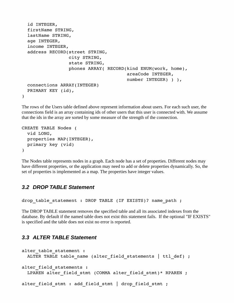
  id INTEGER,  firstName STRING,  lastName STRING,  age INTEGER,  income INTEGER,  address RECORD(street STRING,                 city STRING,                 state STRING,                 phones ARRAY( RECORD(kind ENUM(work, home),                                      areaCode INTEGER,                                      number INTEGER) ) ),  connections ARRAY(INTEGER)  PRIMARY KEY (id),)

The rows of the Users table defined above represent information about users. For each such user, the connections field is an array containing ids of other users that this user is connected with. We assume that the ids in the array are sorted by some measure of the strength of the connection.

CREATE TABLE Nodes (  vid LONG,  properties MAP(INTEGER),  primary key (vid))

The Nodes table represents nodes in a graph. Each node has a set of properties. Different nodes may have different properties, or the application may need to add or delete properties dynamically. So, the set of properties is implemented as a map. The properties have integer values.

3.2 DROP TABLE Statement

drop_table_statement : DROP TABLE (IF EXISTS)? name_path ;

The DROP TABLE statement removes the specified table and all its associated indexes from the database. By default if the named table does not exist this statement fails. If the optional "IF EXISTS" is specified and the table does not exist no error is reported.

3.3 ALTER TABLE Statement

alter_table_statement :  ALTER TABLE table_name (alter_field_statements | ttl_def) ;

alter_field_statements :  LPAREN alter_field_stmt (COMMA alter_field_stmt)* RPAREN ;

alter_field_stmt : add_field_stmt | drop_field_stmt ;

add_field_stmt : ADD name_path type_def default_def? comment? ;

drop_field_stmt : DROP name_path ;

The ALTER TABLE statement allows an application to add or remove a schema field from the table schema. It also allows to change the default TTL value for the table. Adding or dropping a field does not affect the existing rows in the table. If a field is dropped, it will become invisible inside existing rows that do contain the field. If a field is added, its default value or NULL will be used as the value of this field in existing rows that do not contain it.

4 SQL DML: The Query Statement

In the current SQL version, a query is a statement that consists of zero or more variable declarations, followed by single SELECT-FROM-WHERE (SFW) expression:

query :  var_decls? sfw_expr ;

Variable declarations and expressions will be defined later in this chapter. Before doing so, a few general concepts and related terminology must be established first.

4.1 Expressions, sequences, and sequence type

In general, a SQL expression represents a set of operations to be executed in order to produce a result. Expressions are built by combining other (sub)expressions via operators, function calls, or other grammatical constructs. As we will see, the simplest kinds of expressions (having no subexpressions) are constants (aka literals) and references to variables or identifiers.

In SQL, the result of any expression is a sequence of zero or more items (including NULLs). We will refer to such sequences as svalues. Notice that a single item is considered equivalent to a sequence containing that single item.

In the remainder of this chapter we will present the kinds of expressions that are currently supported bySQL. For each expression, we will first show its syntactic form, then define its semantics, and finally give one or more examples of its usage. Part of the semantic definition is to describe the type of the items an expression operates on, and the type of its result set. Given that each expression operates on one or more input sequences and produces a sequence, the concept of a sequence type is useful in this regard. A sequence type specifies the type of items that may appear in a sequence, as well as an indication about the cardinality of the sequence. Specifically, the following syntax is used to specify a sequence type, i.e., a set of svalues:

sequence_type :  “empty_sequence” | item_type cardinality_indicator? ;

item_type : type_def ;

cardinality_indicator : STAR | PLUS | QUESTION ;

empty_sequence is the sequence type containing just one svalue: the empty sequence. The item_type is one of the types in the data model. The cardinality_indicator (a.k.a quantifier) is one of the following:

• * : indicates a sequence of zero or more items• + : indicates a sequence of one or more items• ? : indicates a sequence of zero or one items• The absence of a quantifier indicates a sequence of exactly one item.

The above syntax is not currently available for use in SQL queries. We will use it here for documentation purposes only. Users may also encounter it in error messages and in the printouts of query execution plans.

A subtype relationship exists among sequence types as well. It is defined as follows:

• The empty sequence is a subtype of all other sequence types

• A non-empty sequence type SUB is a subtype of another sequence type SUP if SUP is not the empty sequence, SUB's item type is a subtype of SUP's item type, and SUB's quantifier is a sub-quantifier of SUP's quantifier, where the sub-quantifier relationship is defined by the following table:

Sub Q1 one ? + *

Sup Q2

one true false false false

? true true false false

+ true false true false

* true true true true

In the following sections, when we say that the result of an expression must have (sequence) type T, what we mean is that the result must have type T or any subtype of T. Similarly, the usual subtype-substitution rules applies to input sequences: if an expression expects as input a sequence of type T, anysubtype of T may actually be used as input.

4.2 External variable declarations

var_decls :  DECLARE var_decl SEMICOLON (var_decl SEMICOLON)*;

var_decl :  var_name type_def;

var_name :  DOLLAR id ;

As mentioned already, a query starts with a variables declarations section. The variables declared here are called external variables, and they play the role of the global constant variables found in traditionalprogramming languages (e.g. final static variables in java, or const static variables in c++). However, contrary to java or c++, the values of external variables are not known in advance, i.e. when the query is formulated or compiled. Instead, the external variables must be bound to their actual values before the query is executed. This is done via programmatic APIs Getting Started with Oracle NoSQL Database Tables. The type of the item bound to an external variable must be a subtype of the variable's declared type. The use of external variables allows the same query to be compiled once and then executed multiple times, with different values for the external variables each time.

As we will see later, in addition to external variables, SQL allows for the (sometimes implicit) declaration of internal variables as well. Internal variables are bound to their values during the execution of the expressions that declare them. Variables (internal and external) can be referenced in other expressions by their name. In fact, variable references themselves are expressions, and together with literals, are the starting building blocks for forming more complex expressions.

Each variable is visible (i.e., can be referenced) within a scope. The query as a whole defines the global scope, and external variables exist within this global scope. As we will see, certain expressions create sub-scopes. As a result, scopes may be nested. A variable declared in an inner scope hides another variable with the same name that is declared in an outer scope. Otherwise, within any given scope, all variable names must be unique.

4.2.1 Example:

declare $age  integer;select firstName, lastNamefrom Userswhere age > $age

The above query selects the first and last names of all users whose age is greater than the value assigned to the $age variable when the query is actually executed.

4.3 Select-From-Where (SFW) expression

sfw_expr :  select_clause from_clause where_clause? orderby_clause?;

from_clause : FROM table_name tab_alias? ;

table_name : name_path ;

tab_alias : AS ? DOLLAR? id ;

where_clause : WHERE or_expr ;

select_clause :

  SELECT hints? (STAR |                (or_expr col_alias? (COMMA or_expr col_alias?)*)) ;

hints : '/*+' hint* '*/' ;

hint : ( (PREFER_INDEXES LP name_path index_name* RP) |         (FORCE_INDEX    LP name_path index_name  RP) |         (PREFER_PRIMARY_INDEX LP name_path RP)       |         (FORCE_PRIMARY_INDEX  LP name_path RP) ) STRING?;

col_alias : AS id ;

orderby_clause :  ORDER BY or_expr sort_spec (COMMA or_expr sort_spec)* ;

sort_spec : (ASC | DESC)? (NULLS (FIRST | LAST))? ;

The semantics of the SFW expression are similar to those in SQL. Processing starts with the FROM clause, followed by the WHERE clause (if any), followed by the ORDER BY clause (if any), and finishing with the SELECT clause. Each clause is described below. Notice that in the current SQL version, a query must contain exactly one SFW expression, which is also the top-level expression of thequery. In other words, subqueries are not supported yet.

4.3.1 FROM clause

As shown in the grammar, in the current SQL version, the FROM clause is very simple: it can include only a single table. The table is specified by its name, which may be a composite (dot-separated) name in the case of child tables. The table name may be followed by a table alias. The result of the FROM clause is a sequence containing the rows of the referenced table. The FROM clause creates a nested scope, which exists for the rest of the SFW expression.

The SELECT, WHERE, and ORDER BY clauses operate on the rows produced by the FROM clause, processing one row at a time. The row currently being processed is called the context row. The context row can be referenced in expressions by either the table name, or the table alias (sometimes no explicit reference is needed for “simple” column references). If the table alias starts with a dollar sign ($), then it actually serves as a variable declaration for a variable whose name is the alias. This variable is boundto the context row and can be referenced within the SFW expression, anywhere an expression returninga single record may be used. Notice that if this variable has the same name as an external variable, it hides the external variable.

4.3.2 WHERE Clause

The WHERE clause returns a subset of the rows coming from the FROM clause. Specifically, for each context row, the expression in the WHERE clause is evaluated. The result of this expression must have type BOOLEAN?. If the result is false, or empty, or NULL, the row is skipped; otherwise the row is passed on to the next clause (the ORDER BY, if any, otherwise the SELECT).

4.3.3 ORDER BY clause

The ORDER BY clause reorders the sequence of rows it receives as input. The relative order between any two input rows is determined by evaluating, for each row, the expressions listed in the order-by clause and comparing the resulting values. Each order-by expression must have type ANY_ATOMIC. Let N be the number of order-by expressions and let Vi1, Vi2, … ViN be the atomic values returned by evaluating these expressions, from left to right, on row Ri. Two rows Ri, Rj are considered equal if Vik is equal to Vjk for each k in 1, 2, …, N. In this context, NULLs are considered to be equal only to themselves. Otherwise, Ri is considered less than Rj if there is a pair Vim, Vjm such that:

• m is 1, or Vik is equal to Vjk for each k in 1, 2, …, (m-1), and• Vim is not equal to Vjm, and• Neither of Vim, Vjm is NULL and either (a) Vim is less than Vjm and the m-th sort_spec specifies

ascending order, or (b) Vim is greater than Vjm and the m-th sort_spec specifies descending order, or• Vim is NULL and either (a) the m-th sort_spec specifies ascending order and NULLS FIRST, or (b)

m-th sort_spec specifies descending order and NULLS LAST, or• Vjm is NULL and either (a) the m-th sort_spec specifies ascending order and NULLS LAST, or (b)

m-th sort_spec specifies descending order and NULLS FIRST.

In the above rules, comparison of any two values Vik and Vjk, when neither of them is NULL, is done according to the rules of the value-comparison operators.

The above rules describe the general semantics of the ORDER BY clause. However, the current SQL implementation imposes an important restriction on when ordering can actually be done. Specifically, ordering is possible only if there is an index that already sorts the rows in the desired order. More precisely, let e1, e2, …, eN by the order-by expressions as they appear in the ORDER BY clause (from left to right). Then, there must exist an index (which may be the primary-key index or one of the existing secondary indexes) such that for each i in 1,2,...,N, ei matches the definition of the i-th index field. Furthermore, all the order_specs must specify the same ordering direction and for each sort_spec,the desired ordering with respect to NULLs must match the way NULLs are sorted by the index.

4.3.4 SELECT Clause

The SELECT clause comes in two forms: one containing a single star symbol (*) and the other containing a list of expressions, where each expression is optionally associated with a name. In the second form, we will refer to the listed expressions and their associated names as field expressions and field names respectively.

In its “select star” form, the SELECT clause is a noop; it simply returns its input sequence of rows.

In its “projection” form, the SELECT clause creates a new record for each input row. The new record has one field for each field expression and the fields are arranged in the same order as the field expressions. For each field, its value is the value computed by the corresponding field expression and its name is the name associated with the field expression. If no field name is provided explicitly (via the AS keyword), one is generated internally during query compilation. To create valid records, the field names must be unique. Furthermore, each field expression must have type ANY? (i.e., return at

most one item). If the result of a field expression is empty, NULL is used as the value of the corresponding field in the created record.

The above semantics imply that all records generated by a SELECT clause have the same number of fields and the same field names. As a result, a record type can be created during compilation time that includes all the records in the result set of a query. This record type is the type associated with each created record, and is available programmatically to the application.

The SELECT clause may also contain one or more hints, that help the SQL processor choose an index to use for the query.

4.3.5 Examples

In this section we show some simple SFW examples. More complex examples will be shown in following sections that present other kinds of expressions.

Select all information for all users

select * from Users

Select all information for users whose first name is "John"

select * from Users where firstName = "John"

Select the id and the last name for users whose age is greater than 30. We show 4 different ways of writing this query, illustrating the different ways that the top-level columns of a table may be accessed.

select id, lastName from Users where age > 30

select Users.id, lastName from Users where Users.age > 30

select $u.id, lastName from Users $u where $u.age > 30

select u.id, lastName from Users u where users.age > 30

Select the id and the last name for users whose age is greater than 30, returning the results sorted by id. Sorting is possible in this case because id is the primary key of the users table.

select id, lastName from Users where age > 30 order by id

Select the id and the last name for users whose age is greater than 30, returning the results sorted by age. Sorting is possible only if there is a secondary index on the age column (or more generally, a multi-column index whose first column is the age column).

select id, lastName from Users where age > 30 order by age

4.4 AND and OR logical operators

or_expr : and_expr | or_expr OR and_expr ;

and_expr : comp_expr | and_expr AND comp_expr ;

The and and or binary operators have the usual semantics. Each or their operands must have type BOOLEAN?. An empty result from an operand is treated as the false value. If an operand returns NULL then:• The and operator returns false if the other operand returns false; otherwise, it returns NULL.• The or operator returns true if the other operand returns true; otherwise it returns NULL.

4.4.1 Examples:

Select the id and the last name for users whose age is between 30 and 40 or their income is greater than 100K.

select id, lastNamefrom Userswhere 30 <= age and age <= 40 or income > 100000

4.5 Value comparison operators

comp_expr : add_expr ((val_comp_op | any_comp_op) add_expr)? ;

val_comp_op : "=" | "!=" | ">" | ">=" | "<" | "<=" ;

Each operand of a value comparison operator must have type ANY?. (We call these operators value comparisons because they compare at most one value with at most one other value. This is in contrast to the any comparisons, defined in the next section, which compare two sequences of values). If an operand returns the empty result, the result of the comparison expression is also empty. If an operand returns NULL, the result of the comparison expression is also NULL. Otherwise the result is a boolean value that is computed as follows.

Among atomic items, the following rules apply:

• A numeric item is comparable with any other numeric item. If an integer/long value is compared to a float/double value, the integer/long will first be cast to float/double.

• A string item is comparable to another string item (using the java String.compareTo() method). A string item is also comparable to an enum item. In this case, before the comparison the string is cast to an enum item in the type of the other enum item. Such a cast is possible only if the enum type contains a token whose string value is equal to the source string. If the cast is successful, the two enum items are then compared as explained below; otherwise, an error is raised.

• Two enum items are comparable only if they belong to the same type. If so, the comparison is done

on the ordinal numbers of the two enums (not their string values). As mentioned above, an enum itemis also comparable to a string item, by casting the string to an enum item.

• Binary and fixed binary items are comparable with each other for equality only. The 2 values are equal if their byte sequences have the same length and are equal byte-per-byte.

• A boolean item is comparable with another boolean item, using the java Boolean.compareTo() method.

The semantics of comparisons among complex items are defined in a recursive fashion. Specifically:

• A record is comparable with another record for equality only. To be equal, the 2 records must have equal sizes (number of fields) and for each field in the first record, there must exist a field in the other record such that the two fields are at the same position within their containing records, have equal field names, and equal field values.

• A map is comparable with another map for equality only. To be equal, the 2 maps must have equal sizes (number of entries) and for each entry in the first map, there must exist an entry in the other map such that the two entries have equal keys and equal values.

• An array is comparable to another array. Comparison between 2 arrays is done lexicographically, thatis, the arrays are compared like strings, with the array elements playing the role of the "characters" tocompare.

If two items are not comparable according to the above rules, an error is raised.

4.5.1 Example

We have already seen examples of comparisons among atomic items. Here is an example involving comparison between two arrays:

Select the id and lastName for users who are connected with users 3, 20, and 10 only and in exactly thisorder. In this example, an array constructor is used to create an array with the values 3, 20, and 10, in this order.

select id, lastName from Users where connections = [3, 20, 10]

4.6 Sequence comparison operators

comp_expr : add_expr ((comp_op | any_op) add_expr)? ;

any_comp_op :  "=any" | "!=any" | ">any" | ">=any" | "<any" | "<=any" ;

Comparisons between two sequences is done via another set of operators: =any, !=any, >any, >=any, <any, <=any. These any operators have existential semantics: the result of an any operator on two input

sequences S1 and S2 is true if and only if there is a pair of items i1 and i2, where i1 belongs to S1, i2 belongs to S2, and i1 and i2 compare true via the corresponding value-comparison operator. In contrast to the value comparisons, sequence comparisons do not ever return a NULL or empty result, and do notraise an error if the two sequences contain items that are not comparable to each other via the value comparisons. In other words, sequence comparisons always return true or false.

Notice that since a single item is equivalent to a sequence of one item, the any operators can also be used to compare a single item with another single item. In this case, they behave like the value comparisons, but without raising an error if the two items are not comparable, and converting NULL and empty operands to false results.

4.6.1 Examples

Select the id, lastName and address for users who are connected with the user with id 3. The expressionconnections[] returns a sequence with all the elements of the connections array.

select id, lastName, address from Users where connections[] =any 3

Select the id, lastName and address for users who are connected with any users having id greater than 100.

select id, lastName, address from Users where connections[] >any 100

4.7 Arithmetic expressions

add_expr : multiply_expr ((PLUS | MINUS) multiply_expr)* ;

multiply_expr : unary_expr ((STAR | DIV) unary_expr)* ;

unary_expr : path_expr | (PLUS | MINUS) unary_expr ;

SQL supports the usual arithmetic operations: +, -, *, and /. Each operand to these operators must produce at most one numeric item. If any operand returns the empty sequence or NULL, the result of the arithmetic operation is also empty or NULL, respectively. Otherwise, the operator returns a single numeric item, which is computed as follows:

• If any operand returns a double item, the item returned by the other operand is cast to a double value and the result is a double item that is computed using java's arithmetic on doubles, otherwise,

• If any operand returns a float item, the item returned by the other operand is cast to a float value and the result is a float item that is computed using java's arithmetic on floats, otherwise,

• If any operand returns a long item, the item returned by the other operand is cast to a long value and the result is a long item that is computed using java's arithmetic on longs, otherwise,

• All operands return integer items, and the result is an integer item that is computed using java's arithmetic on ints.

SQL supports the unary + and – operators as well. The unary + is a noop, and the unary – changes the sign of its numeric argument.

4.7.1 Example

For each user show his/her id and the difference between his/her actual income and an income that is computed as a base income plus an age-proportional amount.

declare$baseIncome integer;$ageMultiplier double;select id,       income ­ ($baseIncome + age * $ageMultiplier) as adjustmentfrom Users

4.8 Path expressions

path_expr :  primary_expr (field_step | slice_step | filter_step)* ;

field_step :  DOT (id | string | var_ref | parenthesized_expr | func_call);

filter_step : LBRACK or_expr RBRACK ;

slice_step : LBRACK or_expr? COLON or_expr? RBRACK ;

Path expressions are used to navigate inside complex items. As shown in the syntax, a path expression has an input expression, followed by one or more steps. The input expression must return zero or more complex items (or NULLs). Each step is actually an expression by itself; it takes as input a sequence of complex items and produces zero or more items, which serve as the input to the next step, if any. Each step creates a nested scope, which covers the step itself.

There are 3 kinds of steps, field, slice, and filter steps. All steps iterate over their input sequence, producing zero or more items for each input item. If the input sequence is empty, the result of the step is also empty. Otherwise, the overall result of the step is the concatenation of the results produced for each input item. The input item that a step is currently operating on is called the context item, and it is available within the step expression via an implicitly-declared variable, whose name is a single dollar sign ($). This context-item variable exists in the scope created by the step expression.

For all kinds of steps, if the context item is NULL, it is just propagated into the output sequence. Otherwise, the next 3 sections describe the operation performed by each kind of step on each non-NULL context item.

4.8.1 Field step expressions

field_step :  DOT ( id | string | var_ref | parenthesized_expr | func_call);

In general, a field step selects the value of a field from a record or map, but as explained below, can also operate on arrays that contain records or maps. The field to select is specified by its field name, which is either given explicitly as an identifier, or is computed by a name expression. The name expression, must have type STRING?.

For each context item $:

• If $ is not a complex item, an error is raised.

• The name expression is computed. Let K be the result of of the name expression (if an identifier is used instead of a name expression, K is the string with the same characters as the identifier).

• If K is the empty sequence or NULL, $ is skipped.

• If $ is a record, then if $ contains a field whose name is equal to K, the value of that field is selected, otherwise, an error is raised.

• If $ is a map, then if $ contains an entry whose key is equal to K, the value of that entry is selected, otherwise, $ is skipped.

• If $ is an array, the field step is applied recursively to each element of the array (with the context item being set to the current array element).

4.8.2 Examples

Select the id and the city of users who live in California.

select id, $u.address.cityfrom Users $uwhere $u.address.state = "CA"

Notice that path expressions that start with a table column (address in the above example) must actuallystart with a table name or table alias. Otherwise, an expression like address.city would be interpreted asa reference to the city column of a table called address, which is of course not correct.

Select the first and last name of all users who have a phone number with area code 650. Return the result ordered by city. Notice that in this example the path expression in the WHERE clause returns a sequence of multiple items (area codes). So, we use the =any comparison operator. Remember also thatthe sort is possible only if there is an index on table Users, whose first field is defined by the path expression address.city.

select firstName, lastNamefrom Users $uwhere $u.address.phones.areaCode =any 650order by $u.address.city

Select the value of a specified property for the nodes that have a weight property whose value is 100. The property to display is communicated to the query via the $prop external variable.

declare $prop string;select $v.properties.$prop as propertyfrom Vertex $vwhere $v.properties.weight = 100

For each user, select his/her id and a field from his/her address. The field to select is specified via an external variable.

declare $fieldName string;select $u.id, $u.address.$fieldNamefrom Users $u

Given that the SQL compiler does not know what field is going to be selected, it cannot assign a precise type to the u.address.$fieldName expression. All it can do is assign the type ANY in this case (but notice that the type of the actual items selected by this expression is going to be either STRING or ARRAY(RECORD(...))). Furthermore, the overall type of the query result is not precise any more; it is RECORD(id INTEGER, column_2 ANY), and the record items generated by the query will have this imprecise type as their associated type. (The SQL processor could be constructing on-the-fly a precise RECORD type for each individual record constructed by the query, but it does not do that for performance reasons).

In the current SQL version, a field-step expression whose name expression is not an identifier or string literal, is the only kind of a expression that can result to non-precise types assigned to query expressions and to constructed records. This kind of expression may not be very useful in the current SQL version, but we expect it to become more useful in future versions.

4.8.3 Filter step expressions

filter_step : LBRACK or_expr? RBRACK ;

In general, a filtering step selects elements of arrays or maps by computing a predicate expression for each element and selecting or rejecting the element depending on the predicate result. The result of the filter step is a sequence containing all selected items. If the predicate expression is missing, all the elements are selected. Otherwise, for each context item $:

• If $ is not an array or a map, an error is raised.

• If $ is an array, the step iterates over the array elements and computes the predicate expression on each element. In addition to the context-item variable ($), the predicate expression may reference the following two implicitly-declared variables: $element is bound to the context element, i.e., the current element in $, and $elementPos is bound to the position of the context element within $ (positions are counted starting with 0). The predicate expression must return a boolean item, or a numeric item, or the empty sequence, or NULL. A NULL or an empty result from the predicate expression is treated as a false value. If the predicate result is true/false, the context element is selected/skipped, respectively. If the predicate result is a number P, the context element is selected only if the condition $elementPos = P is true, according to the rules of value comparisons. Notice that this implies that if P is negative or greater or equal to the array size, the context element is

skipped.

• If $ is a map, the step iterates over the map entries and computes the predicate expression on each entry. In addition to the context-item variable ($), the predicate expression may reference the following two implicitly-declared variables: $key is the key of the current map entry (the context entry), and $element is the value of the current entry. The predicate expression must return a booleanitem, or the empty sequence, or NULL. A NULL or an empty result from the predicate expression is treated as a false value. The context element is then skipped/selected if the predicate result is false/true respectively.

4.8.4 Examples:

For each user, select his/her last name and his/her phone numbers with area code 650. Notice the the path expression in the select clause is enclosed in square brackets, which is the syntax used for array-constructor expressions. The array constructor is needed because the path expression may return more than one items; the array constructor converts the sequence of items into an array that contains the sequence items.

select lastName,       [ $u.address.phones[$element.areaCode = 650].number ] as       phoneNumbersfrom Users $u

Notice that without filter-step expressions, we would need to use a subquery to write the above query. Specifically, the query would look like this:

select lastName,       [         select $phone.number         from $u.address.phones as $phone         where $phone.areaCode = 650       ] as phoneNumbersfrom Users AS $u

For each user, select his/her last name and his/her phone numbers having the same area code as the firstphone number of that user. In this query, the context-item variable ($) appearing in the filter step expression [$element.areaCode = $[0].areaCode] refers to the context item of that filter step, i.e., to a phones array as a whole. The context-element variable ($element) refers to an element of that array.

select lastName,       [ u.address.phones[$element.areaCode = $[0].areaCode].number ]from Users u

Among the 10 strongest connections of each user, select the ones with id > 100. (Remember that the connections array is assumed to be sorted by the strength of the connections, with the stronger connections appearing first)

select [ connections[$element > 100 and $elementPos < 10] ] as       interestingConnectionsfrom Users

Select the first and last name of all users who have a phone number with area code 650. Return the result ordered by city. This query is equivalent to the second one of the Example shown above section24. The only difference is in the use of the square brackets in the path expression appearing in the WHERE clause. The queries are equivalent because $u.address.phones.areaCode is just a short-hand for $u.address.phones[].areaCode.

select firstName, lastNamefrom Users $uwhere $u.address.phones[].areaCode =any 650order by $u.address.city

4.8.5 Slice step expressions

slice_step : LBRACK or_expr? COLON or_expr? RBRACK ;

In general, a slice step selects elements of arrays based only on the element positions. The elements to select are the ones whose positions are within a range between a "low" position and a "high" position. The low and high positions are computed by two boundary expressions: a "low" expression for the lowposition and a "high" expression for the high position. Each boundary expression must return at most one item of type LONG or INTEGER, or NULL. The low and/or the high expression may be missing. The context-item variable ($) is available during the computation of the boundary expressions.

For each context item $:

• If $ is not an array, an error is raised.

• Otherwise, the boundary expressions are computed, if present. If any boundary expression returns NULL or an empty result, $ is skipped. Otherwise, let L and H be the values returned by the low and high expressions, respectively. If the low expression is absent, L is set to 0. If the high expression is absent, H is set to the size of the array - 1. If L is < 0, L is set to 0. If H > array_size - 1, H is set to array_size - 1. After L and H are computed, the step selects all the elements between positions L and H (L and H included). If L > H no elements are selected.

Notice that based on the above rules, slice steps are actually a special case of filter steps. For example, a slice step with both boundary expressions present, is equivalent to <input expr>[<low expr> <= $elementPos and $elementPos <= <high expr>]. Slice steps are provided for convenience (and better performance).

4.8.6 Examples:

Select the strongest connection of the user with id 10.

select connections[0] as strongestConnection from Users where id = 10

For user 10, select his/her 5 strongest connections (i.e. the first 5 ids in the "connections" array). Notice that the slice expression will return at most 5 ids; if user 10 has fewer that 5 connections, all of his/her connections will be returned.

select [ connections[0:4] ] as strongConnectionsfrom Userswhere id = 10

For user 10, select his/her 5 weakest connections (i.e. the last 5 ids in the "connections" array). In this example, size() is a function that returns the size of a given array, and $ is the context array, i.e., the array from which the 5 weakest connections are to be selected.

select [ connections[size($) ­ 5 : ] ] as weakConnectionsfrom Userswhere id = 10

4.9 Primary expressions

primary_expr :  const_expr |  column_ref |  var_ref |  array_constructor |  func_call |  parenthesized_expr ;

4.9.1 Constant expressions

const_expr : INT_CONST | FLOAT_CONST | string | TRUE | FALSE ;

string : STRING_CONST | DSTRING_CONST ;

The syntax for INT_CONST, FLOAT_CONST, STRING_CONST, and DSTRING_CONST was given in section 4.

In the current SQL version, a query can contain 4 kinds of constants (a.k.a. literals):

• Strings: sequences of unicode characters enclosed in double or single quotes. String literals are translated into String items.

• Integer numbers: sequences of one or more digits. Integer literals are translated into Integer items, if their value fits in 4 bytes, otherwise into Long items.

• Real numbers : representation of real numbers using “dot notation” and/or exponent. Real literals are translated into Double items.

• The boolean values true and false.

4.9.2 Column references

column_ref : id (DOT id)? ;

A column-reference expression returns the item stored in the specified column within the context row (the row that a WHERE, ORDER BY, or SELECT clause is currently working on). Syntactically, a column-reference expression consists of one identifier, or 2 identifiers separated by a dot. If there are 2 ids, the first is considered to be a table name/alias and the second a column in that table. A single id refers to a column in the table referenced inside the FROM clause.

Notice that child tables in Oracle NoSQL have composite names using dot as a separator among multiple ids. As a result, a child-table name cannot be used in a column-reference expression; instead, a(single-id) alias must be used to access a child table column via the 2-id format.

4.9.3 Variable references

var_ref : DOLLAR id? ;

A variable-reference expression returns the item that the specified variable is currently bound to. Syntactically, a variable-reference expression is just the name of the variable.

4.9.4 Array constructor

array_constructor : LBRACK or_expr (COMMA or_expr)* RBRACK ;

An array constructor constructs a new array out of the items returned by the expressions inside the square brackets. These expressions are computed left to right and the produced items are appended to the array. The element type of the resulting array is set to the type of the first item to be added to the array. If any subsequent item has a different type, an error is raised.

4.9.5 Function calls

func_call : id LPAREN (or_expr (COMMA or_expr)*)? RPAREN ;

Function-call expressions are used to invoke functions, which in the current SQL version can be built-in (system) functions only. Syntactically, a function call starts with an id, which identifies the function to call by name, followed by a parenthesized list of zero or more argument expressions separated by comma.

Each function has a signature, which specifies the sequence type of its result and a sequence type for each of its parameters. Evaluation of a function-call expression starts with the evaluation of each of its arguments. The result of each argument expression must be a subtype of the corresponding parameter type, or otherwise, it must be promotable to the parameter type. In the later case, the argument value will actually be cast to the expected type. Finally, after type checking and any necessary promotions are

done, the function's implementation is invoked with the possibly promoted argument values.

The following type promotions are currently supported:

• INTEGER is promotable to FLOAT or DOUBLE• LONG is promotable to FLOAT or DOUBLE• STRING is promotable to ENUM, but the cast will succeed only if the ENUM type contains a token

whose string value is the same as the input string. The current SQL version implements the following two functions:

• INTEGER? size(item ANY?)Returns the size of a complex item (array, map, record). Although the parameter type appears as ANY?,the runtime implementation of this function raises an error if the given item is not complex. The function accepts an empty sequence as argument, in which case it will return the empty sequence.

• STRING* keys(item ANY?)Returns the keys (field names) of a given record or map. Although the parameter type appears as ANY?, the runtime implementation of this function raises an error if the given item is not a record or map. The function accepts an empty sequence as argument, in which case it will return the empty sequence. Otherwise, it returns a sequence of zero or more strings (an empty map has no keys, but a record has always at least one key).

4.9.6 Parenthesized expressions

parenthesized_expr : LPAREN or_expr RPAREN;

Parenthesized expressions are used primarily to alter the default precedence among operators. They are also used as a syntactic aid to mix expressions in ways that would otherwise cause syntactic ambiguities. An example of the later usage is in the definition of the field_step parse rule. An example of the former usage is this:

Select the id and the last name for users whose age is less or equal to 30 and either their age is greater than 20 or their income is greater than 100K.

select id, lastNamefrom Userswhere (income > 100000 or 20 < age) and age <= 30

5 Indexing in Oracle NoSQL

Roughly speaking, indexes are ordered maps, mapping values contained in the rows of a table back to the containing rows. As such, indexes provided fast access to the rows of a table, when the information we are searching for is contained in the index. In section 31 we define the semantics of the CREATE INDEX statement and describe how the contents of an index are computed. As we will see, Oracle NoSQL comes with rich indexing capabilities, including indexing of deeply nested fields, and indexing of arrays and maps. In section 36 we describe the DROP INDEX statement. Finally, in section 36 we

will see how indexes are used to optimize queries.

5.1 Create Index Statement

create_index_statement :    CREATE INDEX (IF NOT EXISTS)?    index_name ON table_name LPAREN path_list RPAREN comment?;

index_name : id ;

path_list : index_path_expr (COMMA index_path_expr)* ;

index_path_expr : (name_path | keyof_expr | elementof_expr) ;

name_path : id (DOT id)* ;

keyof_expr : KEYOF LP name_path RP ;

elementof_expr : ELEMENTOF LPAREN name_path RPAREN ('.' name_path)?

The create index statement creates an index and populates it with entries computed from the current rows of the specified table. Currently, all indexes in Oracle NoSQL are implemented as B-Trees.

By default if the named index exists the statement fails. However, if the optional "IF NOT EXISTS" clause is present and the index exists and the index specification matches that in the statement, no error is reported. Once an index is created, it is automatically updated by Oracle NoSQL when rows areinserted, deleted, or updated in the associated table.

An index is specified by its name, the name of the table that it indexes, and a list of one or more index paths expressions (or just index paths, for brevity) that specify which table columns or nested fields are indexed and are also used to compute the actual content of the index, as described below. The indexname must be unique among the indexes created on the same table. A create index statement may include an index-level comment that becomes part of the index metadata as uninterpreted text. COMMENT strings are displayed in the output of the "DESCRIBE" statement.

An index stores a number of index entries. Index entries can be viewed as record items having a common record type (the index schema) that contains N+K fields, where N is the number of paths in the path_list and K is the number of primary key columns. The last K fields store values that constitute a primary key “pointing” to a row in the underlying table. Each of the first N fields (called index fields) has an atomic type that is one of the indexable types: numeric types, or string, or enum. Index fields may also store NULL values (actually, indexing NULLs has not been implemented yet). Inthe index schema, the fields appear in the same order as the corresponding index paths in path_list.The index entries are sorted in ascending order. The relative position among any two entries is determined by a lexicographical (string-like) comparison of their field values (with the field values playing the role of the characters in a string).

Indexes can be characterized as simple indexes or multi-key indexes. In both cases, for each table row, the index path expressions are evaluated and one or more index entries are created based on the values

returned by the index path expressions. This is explained later. Notice that the syntax used to specify the index paths is somewhat different than the one used for path expressions in queries1. Specifically, the keywords elementof and keyof are used in the DDL, but not in the DML. However, there is a straightforward mapping from DDL syntax to DML syntax:

• A single name_path is equivalent to table_name.name_path, i.e., it is a DML path expression whose input is a table row and its steps are field steps only, using identifiers as their nameexpression. Normally, these identifiers are schema fields, i.e., field names that appear in the CREATE TABLE statement used to create the associated table. Using the example tables, age and address.state are valid index paths for indexes over the Users table. However, as we will see, name_path identifiers may also be map-entry keys. For example, properties.weight is a valid path for an index over the Nodes table; in this path weight is not a schema field, but instead the name of a property that each node in Nodes may or may not have.

• elementof(name_path) is equivalent to table_name.name_path[].

• elementof(name_path).name_path is equivalent to table_name.name_path[].name_path.

• keyof(name_path) is equivalent to keys(table_name.name_path), but with the extra restriction that only maps (not records) are accepted by the keys function.

To simplify the discussion in the rest of this section, we will assume here that a name_path cannot contain any schema fields that have an array type. We will refer to this restriction as the name-path-restriction. For example, according to this restriction, address.phones.areaCode cannot be used as an index path (because phones is an array field), although it is a valid DML path expression. However, the equivalent elementof(address.phones).areaCode path can be used instead2. As a result, in the context of index creation, use of elementof is the only way to extract the elementsof an array or map. Another consequence of the name-path-restriction is that when evaluated on a table row, a name_path will always return at most one result item.

In the context of index creation, if a name_path returns an empty result, NULL is used as the result instead. For example, the path properties.weight will return an empty result on a node that doesnot have a weight property, but this empty result gets converted to NULL. So, in effect, each name_path returns exactly one item.

5.1.1 Simple indexes

An index is a simple one if:

• Each index path is a simple name_path (no keyof or elementof keywords). Under the name-path-restriction described above, this name_path returns exactly one item per table row.

1 This is because the DDL was defined and released before the DML even existed, so making the DDL syntax the same asthe DML one would be a backwards-incompatible change.

2 In reality, a name_path may contain at most one array-typed schema field, and the resulting index is the same as if the elementof keyword had been used.

• The item returned by each such index path has an indexable atomic type.

We refer to paths that satisfy the above conditions as simple index paths.

Given the above definition, the content of a simple index is computed as follows: For each row R, the index paths are computed and a single index entry is created whose field values are the items returned by the index paths plus the primary-key columns of R. As a result, there is exactly one index entry per table row. Notice that the entries of a simple index over a table T are essentially the result of the following query:

select IP1, …, IPn, PK1, …, PKkfrom T

where IPi is the i-th index path appearing in the CREATE INDEX statement, and PKi is the i-th primary-key column of table T.

5.1.2 Simple index examples

create index idx1 on Users (income)

It creates an index with one entry per user in the Users table. The entry contains the income and id (the primary key) of the user represented by the row.

create index idx2 on Users (address.state, address.city, income)

It creates an index with one entry per user in the Users table. The entry contains the state, city, income and id (the primary key) of the user represented by the row.

create index idx3 on nodes (properties.weight)

Creates an index entry for each node. The entry contains the node's weight, if the nodes does have a weight property, or NULL otherwise.

create index idx4 on nodes (properties.price, properties.weight)

Creates an index entry for each node. The entry contains the node's price, or NULL if the node does nothave a price property, and the node's weight, or NULL if the nodes does not have a weight property.

5.1.3 Multi-key indexes

Mutli-key indexes are used to index all the elements of an array, or all the elements and/or all the keys of a map. As a result, for each table row, the index contains as many entries as the number of elements/entries in the array/map that is being indexed. To avoid an explosion in the number of index entries, only one array/map may be indexed (otherwise, for each table row, we would have to form the cartesian product among the elements/entries or each array/map that is being indexed). A more precise definition for multi-key indexes is given in the rest of this section.

An index is a multi-key index if:

1. There is at least one index path that uses a keyof or elementof keyword. Any such index path will be called a multi-key index path, and the associated index field a multi-key field. The index definition may contain more than one multi-key path, but all multi-key paths must use the same name_path inside their keyof or elementof keyword. Let M be this common name_path. For example, we cannot create an index on Users using both of these paths: elementof(connections) and elementof(address.phones).areaCode, because this is indexing two different arrays in the same index, which is not allowed. On the other hand, we can index both the area codes and the phone kinds of users, that is, the paths elementof(address.phones).areaCode and elementof(address.phones).kind can both appear in the same CREATE INDEX statement, in which case M is the path address.phones.

2. Any non-multi-key index paths must be simple paths, as defined in section 32.

3. The shared path M must specify either an array or a map field and the specified array/map must contain indexable atomic items, or record items, or map items. For example, consider the following table definition:

create table Foo (  id INTEGER,  complex1 RECORD(mapField MAP(ARRAY(MAP(INTEGER)))),  complex2 RECORD(matrix ARRAY(ARRAY(RECORD(a LONG, b LONG)))  primary key(id))

The path expression elementof(complex2.matrix) is not valid, because the complex2.matrix array contains other arrays. Neither is elementof(elementof(complex2.matrix)).a valid, because the syntax allows at most oneelementof or keyof per index path. As a result, we cannot index two arrays/maps where one is nested inside the other. On the other hand, the path elementof(complex1.mapField.someKey).someOtherKey is valid. In this case, M is thepath complex1.mapField.someKey, which specifies an array containing maps. Notice that in this index path, someKey and someOtherKey are map-entry keys. So, although we are indexing arrays that are contained inside maps, and the arrays being indexed contain maps, the path is valid, because it is selecting specific entries from the maps involved rather than indexing all the map entries in addition to all the array entries.

4. If M specifies an array (i.e., the index is indexing an array-valued field):

4.1 If the array contains indexable atomic items, then: 4.1.1 There must be a single multi-key index path of the form elementof(M) (without any

name_path following after the elementof). Again, this implies that we cannot index more than one array in the same index.

4.1.2 In this case, for each table row R, a number of index entries are created as follows: M and the simple index paths (if any) are computed on R. Then, elementof(M) is computed, returning either NULL, if M returned NULL, or all the elements of the array returned by M. Finally, for each value V returned by elementof(M), an index entry is created whose field

values are V and the values of the simple paths. 4.1.3 Any duplicate index entries (having equal field values and the same primary key) created by

the above process are eliminated.

4.2 If the array contains records or maps, then: 4.2.1 There must exist name_paths following elementof(M) in all of the multi-key index

paths. Each of these name_paths must return at most one indexable atomic item. We use Ri to denote this name_path in the i-th multi-key index path.

4.2.2 In this case, for each table row R, a number of index entries are created as follows: M and the simple index paths (if any) are computed on R. Then, elementof(M) is computed, returning either NULL, if M returned NULL, or all the elements of the array returned by M. Next, for each value V returned by elementof(M), one index entry is created as follows: the Ri's are computed on V, returning a single indexable atomic item, and an index entry is created, whose field values are the values of the simple index paths plus the values computed by the Ri's.

4.2.3 Any duplicate index entries (having equal field values and the same primary key) created by the above process are eliminated.

5. If M specifies a map field (i.e., the index is indexing a map-valued field), the index may be indexing only map keys, or only map elements, or both keys and elements. In all cases, the definition of map indexes can be given in terms of array indexes, by viewing maps as arrays containing records with 2 fields: a field with name “key” and value a map key, and a field named “element” and value the corresponding map element (that is, MAP(T) is viewed as ARRAY(RECORD(key STRING, element T))). Then, the 3 valid kinds for map indexes are:

5.1 There is a single multi-key index path using the keyof keyword. Using the array view of maps, keyof(M) is equivalent to elementof(M).key.

5.2 There are one or more multi-key index paths, all using the elementof keyoword. Each of these has the form elementof(M).Ri.. Using the array view of maps, each elementof(M).Ri path is equivalent to elementof(M).element.Ri.

5.3 There is one keyof path and one or more elementof paths. This is just a combination of the 2 previous cases.

5.1.4 Multi-key index examples

In this section we give some examples of multi-key indexes. For each index we also present a query that computes the content of the index. However, the queries shown here are not expressible in the current SQL version.

• create index midx1 on Users (elementof(connections))

Creates an index on the elements of the connections array. The elementof keyword in the above statement is optional. The contents of this index are the results of the following query:

select distinct $connection, $user.idfrom Users as $user, $user.connections[] as $connection

• create index midx2 on Users (address.phones.areaCode, income)

Creates an index on the area codes and income of users. The contents of this index are the results of the following query:

select distinct $phone.areaCode, $user.income, $user.idfrom Users as $user, $user.address.phones[] as $phone

• create index midx3 on Users(address.phones.areaCode, address.phones.kind, income)

Creates an index on the area codes, the phone number kinds, and the income of users. The contents of this index are the results of the following query:

select distinct $phone.areaCode, $phone.kind, $user.income,                $user.idfrom Users as $user, $user.address.phones[] as $phone

• create index midx4 on nodes(keyof(properties), elementof(properties))

Creates an index on the entries (both keys and elements) of the properties map in nodes. The contents of this index are the results of the following query:

select distinct $mapEntry.key, $mapEntry.value, $node.idfrom Nodes as $node,     (select { “key” : $key, “value” : $node.properties.$key }      from keys($node.properties) as $key) as $mapEntry

5.2 Drop index Statement

drop_index_statement :  DROP INDEX (IF EXISTS)? index_name ON table_name ;

The DROP INDEX statement removes the specified index from the database. By default if the named index does not exist this statement fails. If the optional "IF EXISTS" is specified and the index does not exist no error is reported.

5.3 Using indexes for query optimization

In Oracle NoSQL, the query processor can identify which of the available indexes are beneficial for a query and rewrite the query to make use of such an index. “Using” an index means scanning a contiguous subrange of its entries, potentially applying further filtering conditions on the entries within this subrange, and using the primary keys stored in the surviving index entries to extract and return the associated table rows. The subrange of the index entries to scan is determined by the conditions appearing in the WHERE clause, some of which may be converted to search conditions for the index. Given that only a (hopefully small) subset of the index entries will satisfy the search conditions, the

query can be evaluated without accessing each individual table row, thus saving a potentially large number of disk accesses.

Notice that in Oracle NoSQL, the primary-key index is always created by default. Furthermore, if no other index is available, the primary index will be used. In other words, there is no pure “table scan” mechanism; a table scan is equivalent to a scan via the primary-key index.

When it comes to indexes and queries, the query processor must answer two questions:

1. Is an index applicable to a query? That is, will accessing the table via this index be more efficient than doing a full table scan (via the primary index).

2. Among the applicable indexes, which index or combination of indexes is the best to use?

Regarding question (2), the current implementation does not support index anding or index oring. As a result, the query processor will always use exactly one index (which may be the primary-key index). Furthermore, there are no statistics on the number and distribution of values in a table column or nestedfields. As a result, the query processor has to rely on some simple heuristics in choosing among the applicable indexes. In addition, SQL allows for the inclusion of index hints in the queries, which are used as user instructions to the query processor about which index to use.

5.3.1 Finding applicable indexes

To find applicable indexes, the query processor looks at the conditions in the WHERE clause, trying to “match” such predicates with the index paths that define each index. In general the WHERE clause consists of one or more conditions connected with AND or OR operators, forming a tree whose leaves are the conditions and whose internal nodes are the AND/OR operators. Let a predicate be any subtree of this WHERE-clause tree. The query processor will consider only top-level AND predicates, i.e., predicates that appear as the operands of a root AND node. If the WHERE clause does not have an AND root, the whole WHERE expression is considered a single top-level AND predicate. Notice that the query processor does not currently attempt to reorder the AND/OR tree in order to put it in conjunctive normal form. On the other hand, it does flatten the AND/OR tree so that an AND node will not have another AND node as a child, and an OR node will not have another OR node as a child. For example, the expression a = 10 and b < 5 and (c > 10 or c < 0) has 3 top-level AND predicates: a = 10, b < 5, and (c > 10 or c < 0), whereas the expression a = 10 and b< 5 and c > 10 or c < 0 has an OR as its root and the whole of it is considered as a single top-level AND predicate. For brevity, in the rest of this section we will use the term “predicate” to meantop-level AND predicate.

The query processor will consider an index applicable to a query if the query contains at least one index predicate: a predicate that can be evaluated during an index scan, using the content of the currentindex entry only, without the need to access the associated table row. Index predicates are further categorized as start/stop predicates or filtering predicates. A start/stop predicate participates in the establishment of the first/last index entry to be scanned during an index scan. A filtering predicate is applied during the index scan to the entries within the subrange being scanned. If an index is used in a query, its index predicates are removed from the query because they are evaluated by the index scan. We say that index predicates are “pushed to the index”. In the rest of this section we explain applicable indexes further via a number of example queries, and using the indexes from sections 33 and 35.

Q1.

select *from Userswhere 10 < income and income < 20

The query contains 2 index predicates. Indexes idx1, idx2, midx2, and midx4 are all applicable. For index idx1, 10 < income is a start predicate and income < 20 is a stop predicate. For the other indexes, both predicates are filtering predicates. If, say, idx2 were to be used, the subrange to scan is thewhole index. Obviously, idx1 is better than the other indexes in this case. Notice however, that the number of table rows retrieved would be the same whether idx1 or idx2 were used. If midx2 or midx3 were used, the number of distinct rows retrieved would be the same as for idx1 and idx2, but a row would be retrieved as many times as the number of elements in the phones array of that row. Furthermore, in the current implementation the query processor does not eliminate these duplicates, so they would appear in the final query result (multi-)set.

Q2.

select *from Userswhere 20 < income or income < 10

The query contains 1 index predicate, which is the whole WHERE expression. Indexes idx1, idx2, midx2, midx3 are all applicable. For all of them, the predicate is a filtering predicate.

Q3.

select *from Userswhere 20 < income or age > 70

There is no index predicate in this case, because no index has info about user ages.

Q4.

select *from Users uwhere u.address.state = “CA” and u.address.city = “San Jose”

Only idx2 is applicable. There are 2 index predicates, both of which serve as both start and stop predicates.

Q5.

select id, 2*incomefrom Users uwhere u.address.state = “CA” and u.address.city = “San Jose”

Only idx2 is applicable. There are 2 index predicates, both of which serve as both start and stop predicates. In this case, the id and income information needed in the SELECT clause is available in the index. As a result, the whole query can be answered from the index only, with no access to the table. Wesay that index idx2 is a covering index for query Q5. SQL will apply this optimization.

Q6.

select *from Users uwhere u.address.state = “CA” and      u.address.city = “San Jose” and      u.income > 10

idx1, idx2, midx2, and midx3 are applicable. For idx2, there are 3 index predicates: the state and city predicates serve as both start and stop predicates; the income predicate is a start predicate. For idx1 only the income predicate is applicable, as a start predicate. For midx2 and midx3, the income predicateis a filtering one.

Q7.

select *from Users uwhere u.address.state = “CA” and      u.income > 10

idx1, idx2, midx2, and midx3 are applicable. For idx2, there are 2 index predicates: the state predicate serves as both start and stop predicate; the income predicate is a filtering predicate. The income predicate is a start predicate for idx1 and a filtering predicate for midx2 and midx3.

Q8.

declare$city string;select *from Users uwhere u.address.state = “CA” and      u.address.city = $city and      (u.income > 50 or (10 < income and income < 20)  

idx1, idx2, midx2, and midx3 are applicable. For idx2, there are 3 index predicates. The state and city predicates serve as both start and stop predicates. The composite income predicate is a filtering predicate for all the applicable indexes (it's rooted at an OR node).

As the above examples indicate, a predicate will be used as a start/stop predicate for an index IDX only if:

• It is of the form <path expr> op <const expr> or <const expr> op <psth expr>• op is a comparison operator• <const expr> is an expression built from literals and external variables only (does not reference any

tables or internal variables)• <path expr> is a path expression that is “matches” an index path P appearing in the CREATE INDEX

statement for IDX (after P is converted to the DML syntax from the DDL syntax). So far we have seen examples of exact matches only. In the examples below we will see some non-exact matches as well.

• If P is not IDX's 1st index path, there are equality start/stop predicates for each index path appearing before P in IDX's definition.

• The comparison operator may be one of the “any” operators. Such operators are matched against the multi-key index paths of multi-key indexes. As shown in the examples below, additional restrictions apply for such predicates.

Q9.

select *from users uwhere u.connections[] =any 10

midx1 is applicable and the predicate is both a start and a stop predicate. No duplicates are returned, because there can be at most one index entry with value 10 per row.

Q10.

select *from users uwhere u.connections[0:4] =any 10

midx1 is applicable. The predicate to push down to mdx1 is u.connections[] =any 10, in order to eliminate users who are not connected at all with user 10. However, the original predicate (u.connections[1:4] =any 10 ) must be retained in the query to eliminate users who do have a connection with user 10, but not among their 5 strongest connections. This is an example where the query path expression does not match exactly the corresponding index path.

Q11.

select *from users uwhere u.connections[] >any 10

midx1 is applicable and the predicate is a start predicate. Duplicates may be returned if the index is used, because there can be more than one index entries greater than 10 per row.

Q12.

select idfrom users uwhere 10 <any u.connections[] and u.connections[] <any 100

midx1 is applicable, but although each predicate by itself is an index predicate, only one of them can actually be used as such. To see why, first notice that the query asks for users that have a connection

with id greater than 10 and another connection (which may or may not be the same as the 1st one) withid less than 100. Next, consider a Users table with only 2 users (say with ids 200 and 500) having the following connections arrays respectively: [ 1, 3, 110, 120 ] and [1, 50, 130]. Both of these arrays satisfy the predicates in Q11, and both users should be returned as a result. Now, consider midx1; it contains the following 7 entries:

{1, 200}, {1, 500}, {3, 200}, {50, 500}, {110, 200}, {120, 200}, {130, 500}

By using only the 1st predicate as a start predicate to scan the index, and applying the 2nd predicate on the rows returned by the index scan, the result of the query is 500, 200, 200, 500, which is correct, modulo the duplicates. If on the other hand both predicates were used for the index scan, only entry {50, 500} would qualify, and the query would return only user 500.

The “problem” here is that the current SQL version does not have an expression that would allows us toapply more than one conditions on the same element of an array (or the same entry of a map). For example a query like this is not currently possible:

select idfrom Users uwhere some $element in u.connections[] satisfies      10 < $element and $element < 100.

The result of this query is user 500 only and both predicates can be used as index predicates (start and stop) . However, in the absence of general “existentially quantified” expressions like the one above,at most one “any” predicate can be pushed to a multi-key index.

Q13.

select *from Users uwhere u.address.phones.areaCode =any 650 and      u.address.phones.kind =any work and      income > 10

This query has the same “problem” as Q10 above. It looks for users whose income is greater than 10, and have a phone number with area code 650, and also have a work phone number (whose area code may not be 650). Index midx3 is applicable, but the address.phones.kind predicate cannot be used as an index predicate. Only the areaCode predicate can be used as a start/stop predicate and the income predicate as a filtering one. Given that no predicate can be pushed to the address.phones.kind index path, midx3 is not really useful for queries in the current SQL version (midx3 can still be “queried” directly, via programmatic APIs). Indexes idx1, idx2, and midx2 are also applicable in Q11.

Q14.

select *from Nodeswhere properties.price = 10

idx4 is applicable and the predicate is both a start and a stop predicate. midx4 is also applicable. To use midx4, two predicates must be pushed to it, even though only one appear in the query. The 1st predicate

is on the “key” index field and the second on the “element” field. Specifically, the predicates key = “price” and element = 10 are pushed as start/stop predicates. This is another example where the match between the query path expression and an index path is not exact: we match properties.price with the elementof(properties) index path, and additionally, generate an index predicate for the keyof(properties) index path.

Q15.

select *from Nodeswhere properties.length = 10 and properties.height > 10

midx4 is applicable. Each of the query predicates is by itself an index predicate and can be pushed to midx4 the same way as the properties.price predicate in the previous example. However, the query predicates cannot be both pushed (at least not in the current implementation). SQL has to choose one of them to push and the other will remain in the query. Because the properties.length predicate is an equality one, it's most likely more selective than the greater-than predicate and SQL will use that.

5.3.2 Choosing the best applicable index

As mentioned already, to choose an index for a query, the query processor uses a simple heuristic together with any user-provided index hints. There are 2 kinds of hints: a FORCE_INDEX hint and a PREFER_INDEXES hint. The FORCE_INDEX hint specifies a single index and the query is going to use that index without considering any of the other indexes (even if there are no index predicates for the force index). However, if the query has an order by and the forced index is not the sorting index, an error will be thrown. The PREFER_INDEXES hint specifies one or more indexes. The query processormay or may not use one of the preferred indexes. Specifically, in the absence of a forced index, index selection works as follows. The FORCE_INDEX and PREFER_INDEXES hints specified indexes by their name. Since the primary index has no explicit name, 2 more hints are available to force or to prefer the primary index: FORCE_PRIMARY_INDEX and PREFER_PRIMARY_INDEX. Hints are inserted in the query as a special kind of comment that appears immediately after the SELECT keyword. Here is the relevant syntax:

select_clause :  SELECT hints? ( STAR |                  (or_expr col_alias (COMMA or_expr col_alias)*) ) ;

hints : '/*+' hint* '*/' ;

hint : ( (PREFER_INDEXES LP name_path index_name* RP) |         (FORCE_INDEX    LP name_path index_name  RP) |         (PREFER_PRIMARY_INDEX LP name_path RP)       |         (FORCE_PRIMARY_INDEX  LP name_path RP) ) STRING?;

The '+' character immediately after (with no spaces) the comment opening sequence ('/*') is what turns the comment into a hint. The string at the end of the hint is just for informational purposes (a comment for the hint) and does not play any role in the query execution.

Unless a index is forced via a FORCE hint, the query processor uses the heuristic to assign a score to each applicable index and then chooses the one with the highest score. If two or more indexes have the same score, the index chosen is the one whose name is alphabetically before the others. In general, preferred indexes will get high scores, but it is possible that other indexes may still win. Describing the details of the heuristic is beyond the scope of this document, but a few high-level decisions are worth mentioning:

• If the query has a complete primary key, the primary index is used.• If the query has a complete shard key, the primary index is used. Using the primary index in this case

implies that a single table partition (in a single shard) will be scanned (because all the qualifying rows will be in that single partition). Using any other index in this case would require sending the query to all the shards and potentially scanning a lot of data on those shard for no good reason. However, if the query has an order by and the primary index is not the sorting index, an error will be thrown.

• If the query has an order by and the previous bullets do not apply, the sorting index is used, even if other indexes may be more selective.

• If none of the previous bullets apply, indexes that are preferred (via a PREFER hint), covering, or have a complete key (i.e., there is an equality predicate on each of its index fields) get high stores andwill normally prevail over other indexes.

6 Appendix : The full SQL grammar

program :    (    query  | create_table_statement  | alter_table_statement  | drop_table_statement  | create_index_statement  | drop_index_statement  | create_text_index_statement  | create_user_statement  | create_role_statement  | drop_role_statement  | drop_user_statement  | alter_user_statement  | grant_statement  | revoke_statement  | describe_statement  | show_statement)    EOF  ;

query : var_decls? sfw_expr ;

var_decls : DECLARE var_decl SEMICOLON (var_decl SEMICOLON)*;

var_decl : var_name type_def;

var_name : DOLLAR id ;

sfw_expr : select_clause from_clause where_clause? orderby_clause?;

from_clause : FROM table_name tab_alias? ;

table_name : name_path ;

tab_alias : AS? DOLLAR? Id

where_clause : WHERE or_expr ;

select_clause :  SELECT hints? ( STAR |                  (or_expr col_alias (COMMA or_expr col_alias)*) ) ;

hints : '/*+' hint* '*/' ;

hint : ( (PREFER_INDEXES LP name_path index_name* RP) |         (FORCE_INDEX    LP name_path index_name  RP) |         (PREFER_PRIMARY_INDEX LP name_path RP)       |         (FORCE_PRIMARY_INDEX  LP name_path RP) ) STRING?;

col_alias : AS id ;

orderby_clause :  ORDER BY or_expr sort_spec (COMMA or_expr sort_spec)* ;

sort_spec : (ASC | DESC)? (NULLS (FIRST | LAST))? ;

or_expr : and_expr | or_expr OR and_expr ;

and_expr : comp_expr | and_expr AND comp_expr ;

comp_expr : add_expr ((val_comp_op | any_comp_op) add_expr)? ;

val_comp_op : "=" | "!=" | ">" | ">=" | "<" | "<=" ;

any_comp_op :  "=any" | "!=any" | ">any" | ">=any" | "<any" | "<=any" ;

add_expr : multiply_expr ((PLUS | MINUS) multiply_expr)* ;

multiply_expr : unary_expr ((STAR | DIV) unary_expr)* ;

unary_expr : path_expr | (PLUS | MINUS) unary_expr ;

path_expr :  primary_expr (field_step | slice_step | filter_step)* ;

field_step :  DOT (id | string | var_ref | parenthesized_expr | func_call);

filter_step : LBRACK or_expr RBRACK ;

slice_step : LBRACK or_expr? COLON or_expr? RBRACK ;

primary_expr :  const_expr |  column_ref |  var_ref |  array_constructor |  func_call |  parenthesized_expr ;

const_expr : INT_CONST | FLOAT_CONST | string | TRUE | FALSE ;

column_ref : id (DOT id)? ;

var_ref : DOLLAR id? ;

array_constructor : LBRACK or_expr (COMMA or_expr)* RBRACK ;

func_call : id LPAREN (or_expr (COMMA or_expr)*)? RPAREN ;

parenthesized_expr : LPAREN or_expr RPAREN;

create_table_statement :  CREATE TABLE (IF NOT EXISTS)? table_name comment?  LPAREN table_def RPAREN ;

table_name : name_path;

table_def : (field_def | key_def) (COMMA (field_def | key_def))* ;

key_def :  PRIMARY KEY  LPAREN (shard_key_def COMMA?)? id_list_with_size? RPAREN ttl_def? ;

id_list_with_size : id_with_size (COMMA id_with_size)* ;

id_with_size : id storage_size? ;

storage_size : LPAREN INT_CONST RPAREN ;

shard_key_def : SHARD LPAREN id_list_with_size RPAREN;

ttl_def : USING TTL INT_CONST (HOURS | DAYS) ;

drop_table_statement : DROP TABLE (IF EXISTS)? name_path ;

alter_table_statement :  ALTER TABLE name_path (alter_field_statements | ttl_def);

alter_field_statements :  LPAREN alter_field_stmt (COMMA alter_field_stmt)* RPAREN ;

alter_field_stmt :add_field_stmt | drop_field_stmt ;

add_field_stmt : ADD name_path type_def default_def? comment? ;

drop_field_stmt : DROP name_path ;

create_index_statement :    CREATE INDEX (IF NOT EXISTS)?    index_name ON table_name LPAREN path_list RPAREN comment?;

index_name : id ;

path_list : index_path_expr (COMMA index_path_expr)* ;

index_path_expr : (name_path | keyof_expr | elementof_expr) ;

keyof_expr : KEYOF LP name_path RP ;

elementof_expr : ELEMENTOF LPAREN name_path RPAREN ('.' name_path)?

name_path : id (DOT id)* ;

type_def :  INTEGER |  LONG |  FLOAT |  DOUBLE |  STRING |  enum_def |  binary_def |  BOOLEAN |  record_def |  array_def |  map_def ;

enum_def : ENUM LPAREN id_list RPAREN ;

binary_def : BINARY (LPAREN INT_CONST RPAREN)? ;

map_def : MAP LPAREN type_def RPAREN ;

array_def : ARRAY LPAREN type_def RPAREN ;

record_def : RECORD LPAREN field_def (COMMA field_def)* RPAREN ;

field_def : id type_def default_def? comment? ;

default_def :  (default_value (NOT NULL)?) | (NOT NULL default_value?) ;

comment : COMMENT string ;

default_value : DEFAULT (number | string | TRUE | FALSE | id) ;

number : MINUS? (FLOAT_CONST | INT_CONST) ;

string : STRING_CONST | DSTRING_CONST ;

id_list : id (COMMA id)* ;

id : ID | ADD | ALTER | AND | ARRAY | AS | ASC | BINARY | BOOLEAN | BY | COMMENT | CREATE | DEFAULT | DESC | DOUBLE | DROP | EXISTS | FIRST | FLOAT | FROM | ENUM | IF | INDEX | INTEGER | KEY | LAST | LONG | MAP | NOT | NULLS | ON | OR | ORDER | PRIMARY | RECORD | SELECT | SHARD | STRING | TABLE | WHERE; ID : ALPHA (ALPHA | DIGIT | '_')* ;

fragment ALPHA : 'a'..'z'|'A'..'Z' ;

fragment DIGIT : '0'..'9' ;

INT_CONST : DIGIT+ ;

FLOAT_CONST : ( DIGIT* '.' DIGIT+ ([Ee] [+­]? DIGIT+)? ) |              ( DIGIT+ [Ee] [+­]? DIGIT+ ) ;

STRING_CONST : '\'' ((ESC) | .)*? '\'' ; // string with single quotes

DSTRING_CONST : '"' ((ESC) | .)*? '"' ;  // string with double quotes

fragment ESC : '\\' ([\'\\/bfnrt] | UNICODE) ;

fragment DSTR_ESC : '\\' (["\\/bfnrt] | UNICODE) ;

fragment UNICODE : 'u' HEX HEX HEX HEX ;

TRUE : [Tt][Rr][Uu][Ee] ;

FALSE : [Ff][Aa][Ll][Ss][Ee] ;