PAPER • OPEN ACCESS

Optomechanical parameter estimationTo cite this article: Shan Zheng Ang et al 2013 New J. Phys. 15 103028

 

View the article online for updates and enhancements.

You may also likeOn multidimensional generalizedCramér–Rao inequalities, uncertaintyrelations and characterizations ofgeneralized q-Gaussian distributionsJ F Bercher

-

Non-asymptotic analysis of quantummetrology protocols beyond theCramér–Rao boundJesús Rubio, Paul Knott and JacobDunningham

-

The lower timing resolution bound forscintillators with non-negligible opticalphoton transport time in time-of-flight PETRuud Vinke, Peter D Olcott, Joshua WCates et al.

-

Recent citationsWeak-force sensing in optomechanicalsystems with Kalman filteringBeili Gong et al

-

Tight Bounds on the SimultaneousEstimation of Incompatible ParametersJasminder S. Sidhu et al

-

Photonic quantum metrologyEmanuele Polino et al

-

This content was downloaded from IP address 220.71.209.156 on 04/01/2022 at 09:58

Optomechanical parameter estimation

Shan Zheng Ang1, Glen I Harris2, Warwick P Bowen2

and Mankei Tsang1,3,4

1 Department of Electrical and Computer Engineering, National University ofSingapore, 4 Engineering Drive 3, Singapore 117583, Singapore2 Centre for Engineered Quantum Systems, University of Queensland, St Lucia,QLD 4072, Australia3 Department of Physics, National University of Singapore, 2 Science Drive 3,Singapore 117551, SingaporeE-mail: eletmk@nus.edu.sg

New Journal of Physics 15 (2013) 103028 (17pp)Received 5 August 2013Published 28 October 2013Online at http://www.njp.org/doi:10.1088/1367-2630/15/10/103028

Abstract. We propose a statistical framework for the problem of parameterestimation from a noisy optomechanical system. The Cramer–Rao lower boundon the estimation errors in the long-time limit is derived and comparedwith the errors of radiometer and expectation–maximization (EM) algorithmsin the estimation of the force noise power. When applied to experimentaldata, the EM estimator is found to have the lowest error and follow theCramer–Rao bound most closely. Our analytic results are envisioned to bevaluable to optomechanical experiment design, while the EM algorithm, withits ability to estimate most of the system parameters, is envisioned to be usefulfor optomechanical sensing, atomic magnetometry and fundamental tests ofquantum mechanics.

4 Author to whom any correspondence should be addressed.

Content from this work may be used under the terms of the Creative Commons Attribution 3.0 licence.Any further distribution of this work must maintain attribution to the author(s) and the title of the work, journal

citation and DOI.

New Journal of Physics 15 (2013) 1030281367-2630/13/103028+17$33.00 © IOP Publishing Ltd and Deutsche Physikalische Gesellschaft

2

Contents

1. Introduction 22. Experiment 33. Theory 4

3.1. Continuous-time model . . . . . . . . . . . . . . . . . . . . . . . . . . . . . . 43.2. Binary hypothesis testing . . . . . . . . . . . . . . . . . . . . . . . . . . . . . 43.3. Cramer–Rao bound . . . . . . . . . . . . . . . . . . . . . . . . . . . . . . . . 6

4. Parameter estimation algorithms 74.1. Averaging . . . . . . . . . . . . . . . . . . . . . . . . . . . . . . . . . . . . . 74.2. Radiometer . . . . . . . . . . . . . . . . . . . . . . . . . . . . . . . . . . . . 74.3. Expectation–maximization (EM) algorithm . . . . . . . . . . . . . . . . . . . 8

5. Application to experimental data 95.1. Procedure . . . . . . . . . . . . . . . . . . . . . . . . . . . . . . . . . . . . . 95.2. Results . . . . . . . . . . . . . . . . . . . . . . . . . . . . . . . . . . . . . . . 10

6. Outlook 12Acknowledgments 13Appendix. EM algorithm for the complex Gauss–Markov model 13References 15

1. Introduction

There has been spectacular technological advances in the use of high-quality optomechanicaloscillators for force sensing, enabling ultra-sensitive force measurements of single spin, charge,acceleration, magnetic field and mass [1–5]. Such advances have opened up the excitingpossibility of experimentally studying quantum light–matter interactions in macroscopicstructures [6, 7], hence paving the way toward new technologies for quantum informationscience and metrology [8–11].

Thermal and measurement noises impose major limitations to the accuracy of mechanicalforce sensors. Furthermore, while the development of higher quality and lower mass mechanicaloscillators has played a central role in advancing the sensitivity of optomechanical forcesensors [12]; such oscillators also have increased sensitivity to their environment. Thisintroduces new sources of noise that can cause fluctuations in parameters, such as the effectiveoscillator temperature and mechanical resonance frequency. As optomechanical technologycontinue to advance, it can be expected that methods to characterize, monitor and control theseadditional noise sources, in conjunction with thermal and measurement noise, will becomeincreasingly important. In this context, statistical signal processing techniques that are provablyoptimal in a theoretical sense offer the potential to improve the actual sensing performancesignificantly, beyond the heuristic curve-fitting procedures commonly employed in the field.

In this paper, we introduce a statistical framework to study the problem of parameterestimation from a noisy optomechanical system. This problem is especially relevant to therecent optomechanics experiments reported in [12, 13]. We derive analytic expressions for theCramer–Rao lower bound on the estimation errors and apply various estimation techniques to

New Journal of Physics 15 (2013) 103028 (http://www.njp.org/)

3

experimental data to estimate the parameters of an optomechanical system, including the forcepower, mechanical resonance frequency, damping rate and measurement noise power.

Our analytic results provide convenient expressions of the estimation errors as a function ofsystem parameters and measurement time and should be valuable to optomechanical experimentdesign. Another highlight of our study is the use of the expectation–maximization (EM)algorithm [14–16], which is generalized here for a complex Gauss–Markov model and appliedto a cavity optomechanical system, both for the first time to our knowledge. Among theestimators we have studied, including the one used in [12, 13], we find that the root-mean-square errors of the EM algorithm in estimating the force noise power are the lowest, followingthe Cramer–Rao bound most closely and beating the estimator in [12, 13] by more than a factorof 5 for longer measurement times.

Our framework is also naturally applicable to quantum systems that can be described bya homogeneous Gauss–Markov model [17], such as quantum optomechanical systems [18–22]and atomic spin ensembles [23, 24]. This makes our study, and the EM algorithm in particular,relevant not only just to future precision sensing and system identification applications but alsoto fundamental tests of quantum mechanics [18, 19, 25].

2. Experiment

To motivate our theoretical model and numerical analysis, we first describe the optomechanicalexperiment presented in [13] that was used to produce the data. The transducer underconsideration consists of a room temperature microtoroidal resonator that simultaneouslysupports mechanical modes sensitive to external forces and high quality optical modes thatpermit ultra-precise readout of the mechanical displacement. We couple shot-noise limited1550 nm laser light into a whispering gallery mode of the microtoroid via a tapered optical fiberwhich is nested inside an all fiber interferometer. Excitation of the mechanical mode, which hasfundamental frequency, damping rate and effective mass of �m = 40.33 MHz, γ = 23 kHz andmeff = 7 ng, respectively, induces phase fluctuations on the transmitted light which is measuredby shot-noise limited homodyne detection. To maintain constant coupling of optical powerinto the microtoroid we use an amplitude and phase modulation technique to actively lock thetoroid-taper separation [26] and laser frequency, respectively. The relative phase of the brightlocal oscillator to the signal is controlled via a piezoactuated fiber stretcher that precisely tunesthe optical path length in one arm of the interferometer. To specifically demonstrate powerestimation, a small incoherent signal is applied to the mechanical oscillator in addition to thethermal fluctuations. This is achieved by the electrostatic gradient force applied by a nearbyelectrode driven with white noise from a signal generator [27].

The measurement record is acquired from the homodyne signal by electronic lock-in detection which involves demodulation of the photocurrent at the mechanical resonancefrequency allowing real time measurement of the slowly evolving quadratures of motion,denoted I (t) and Q(t) where x(t)= I (t)cos(�mt)+ Q(t)sin(�mt). The room temperaturethermal fluctuations of the mechanical mode are observed with a signal-to-noise ratio of 37 dBand calibrated via the optical response to a known reference modulation [28]. The resultingforce sensitivity, which can be extracted from Fourier analysis of the measurement record, willdepend on the specific protocol used. Here we evaluate the force sensitivity of three parameterestimation protocols relative to the Cramer–Rao lower bound.

New Journal of Physics 15 (2013) 103028 (http://www.njp.org/)

4

3. Theory

3.1. Continuous-time model

A simple linear Gaussian model for the mechanical mode can be described by the followingequation for the complex analytic signal z(t) of the mechanical-mode displacement:

dz(t)

dt= −γ z(t)+ i�z(t)+ ξ(t), (1)

where � is the mechanical resonance frequency relative to �m, γ is the damping rate and ξ(t)is the stochastic force as a sum of the thermal noise and the signal. ξ(t) is assumed to be acomplex zero-mean white Gaussian noise [29] with power A and covariance function

E[ξ(t)ξ ∗(t ′)] = Aδ(t − t ′), E[ξ(t)ξ(t ′)] = 0. (2)

The measurements can be modeled in continuous time as

y(t)= Cz(t)+ η(t), (3)

where C is a real parameter and η(t) is the measurement noise, assumed to be a complex additivewhite Gaussian noise with power R:

E[η(t)η∗(t ′)] = Rδ(t − t ′), E[η(t)η(t ′)] = 0. (4)

We assume that the parameters

θ = (�, γ, A,C, R)> (5)

are constant in time, such that z(t), ξ(t), y(t) and η(t) are stationary stochastic processes givenθ . y(t), in particular, has a power spectrum given by

Sy(ω|θ)≡ limT →∞

E

[1

T

∣∣∣∣∫ T/2

−T/2dt y(t) exp(−iωt)

∣∣∣∣2]

(6)

= AS(ω)+ R, (7)

S(ω)≡C2

(ω−�)2 + γ 2. (8)

Although this simple model suffices to describe our experiment, it is not difficult to generalizeour entire formalism to describe more complicated dynamics and colored noise [30]. This isdone by generalizing z(t) to a vector of state variables for more mechanical and optical modes,equation (1) to a vectoral equation of motion, and the parameters (�, γ, A,C, R) to matricesthat describe the coupled-mode dynamics and the noise statistics.

3.2. Binary hypothesis testing

Although hypothesis testing [16, 29] is not the focus of our study, the theory is useful for thederivation of the Cramer–Rao bound, so we present the topic here briefly for completeness.

Suppose that there are two hypotheses, denoted by H0 and H1, with prior probabilitiesP0 and P1 = 1 − P0. From a measurement record Y , with a probability density P(Y |H0) orP(Y |H1) that depends on the hypothesis, one wishes to decide which hypothesis is true.

New Journal of Physics 15 (2013) 103028 (http://www.njp.org/)

5

Given the densities and a decision rule, one can compute Pjk , the probability that Hj is chosenwhen Hk is true. The average error probability is

Pe ≡ P10 P0 + P01 P1. (9)

Pe can be minimized using a Bayes likelihood-ratio test

3≡P(Y |H1)

P(Y |H0)

H1

≷H0

P0

P1, (10)

which means that H1 is chosen if 3> P0/P1 and vice versa. The resulting Pe is often difficultto compute analytically, but can be bounded by upper and lower bounds. For P0 = P1 = 1/2[16, 31],

1

2

[1 −

√1 − F2(0.5)

]6min Pe ≤

1

2min

06s61F(s), (11)

where the upper bound is the Chernoff bound,

F(s)≡ E[3s|H0] =

∫dY P(Y |H0)

[P(Y |H1)

P(Y |H0)

]s

, (12)

and F(0.5) is known as the Bhattacharyya distance between the two probability densities [31].Let Y be a record of continuous measurements

Y = {x(t); −T/26 t 6 T/2}. (13)

If x(t) is a realization of a real zero-mean stationary process with spectrum Sx(ω|Hj), theexponent of F(s) in the case of stationary processes and long observation time (SPLOT) isknown to be [16]

0F ≡ limT →∞

−1

Tln F(s) (14)

=1

2

∫∞

−∞

dω

2πln

sSx(ω|H0)+ (1 − s)Sx(ω|H1)

Ssx(ω|H0)S1−s

x (ω|H1). (15)

This expression means that F(s) has the form of

F(s)= β(T ) exp (−0F T ) , (16)

where −lnβ(T ) is asymptotically smaller than T

limT →∞

−1

Tlnβ(T )= 0, (17)

and therefore β(T ) decays more slowly than exp(−0F T ).For the model in section 3.1, y(t) is a complex signal, and (15) needs to be modified. This

can be done by assuming that y(t) is band limited in [−πb, πb] and considering a real signalx(t) given by

x(t)≡ y(t) exp(iω0t)+ y∗(t) exp(−iω0t), (18)

where ω0 is a carrier frequency assumed to be >πb. We then have

Sx(ω|Hj)= Sy(ω−ω0|Hj)+ Sy(−ω−ω0|Hj). (19)

Using this expression in (15) leads to another expression for the Chernoff exponent given by

0F =

∫ πb

−πb

dω

2πln

sSy(ω|H0)+ (1 − s)Sy(ω|H1)

Ssy(ω|H0)S1−s

y (ω|H1). (20)

Note the absence of the 1/2 factor in (20) compared with (15).

New Journal of Physics 15 (2013) 103028 (http://www.njp.org/)

6

3.3. Cramer–Rao bound

We now consider the estimation of θ from Y with a probability density given by P(Y |θ).Defining the estimate as θ (Y ), the error covariance matrix is

6(θ)≡ E{

[θ (Y )− θ ][θ (Y )− θ ]>∣∣∣θ} , (21)

E[g(Y )|θ ] ≡

∫dY P(Y |θ)g(Y ). (22)

Assuming that θ satisfies the unbiased condition

E[θ (Y )

∣∣∣θ] = θ, (23)

the Cramer–Rao bound on 6 is [16]

6(θ)> J −1(θ), (24)

where J (θ) is known as the Fisher information matrix

J (θ)≡ E{∇ [ln P(Y |θ)] ∇

> [ln P(Y |θ)]∣∣∣θ} , (25)

∇ ≡

(∂

∂θ1,∂

∂θ2, . . .

)>

. (26)

It turns out that J (θ) can be related to the Bhattacharyya distance in a hypothesis testing problemwith

P(Y |H0)= P(Y |θ), (27)

P(Y |H1)= P(Y |θ ′). (28)

F(s) defined in (12) becomes a function of θ and θ ′, and J (θ) can be expressed as [29]

J (θ)= −4∇∇> ln F(0.5, θ, θ ′)

∣∣∣θ ′=θ

. (29)

For the model in section 3.1, y(t) is a realization of a stationary process given θ , so J (θ) forthe estimation of θ from Y = {y(t); −T/26 t 6 T/2} in the SPLOT case can be obtained bycombining (20) and (29):

0j ≡ limT →∞

J (θ)

T(30)

= 4∇∇>

∫ πb

−πb

dω

2πln

Sy(ω|θ)+ Sy(ω|θ ′)

2√

Sy(ω|θ)Sy(ω|θ ′)

∣∣∣∣θ ′=θ

, (31)

where Sy(ω|θ) is given by (6). This expression means that J (θ) for any stationary-processparameter estimation problem increases linearly with time as T → ∞, in the sense of

J (θ)= 0J T + o(T ), (32)

where o(T ) is asymptotically smaller than T :

limT →∞

o(T )

T= 0. (33)

New Journal of Physics 15 (2013) 103028 (http://www.njp.org/)

7

In the asymptotic limit, maximum-likelihood (ML) estimation can attain the Cramer–Raobound [15], so the bound is a meaningful indicator of estimation error. Despite the asymptoticassumption, the simpler analytic expressions are more convenient to use for experimental designpurposes.

Although the preceding formalism is applicable to the estimation of any of the parameters,in the following we focus on A, the force noise power. The Cramer–Rao bound on the mean-square estimation error 6A is

6A ≡ E

{[ A(Y )− A]2

∣∣∣∣θ}> J −1A , (34)

0A ≡ limT →∞

JA

T=

∫ πb

−πb

dω

2π

S2(ω)

[AS(ω)+ R]2. (35)

This bound allows us to investigate the efficiency of the parameter estimation algorithmspresented in the next section.

4. Parameter estimation algorithms

4.1. Averaging

We first consider the estimator used in [12, 13]

Aavg = G∫ T/2

−T/2dt |y(t)|2, G =

[T

∫ πb

−πb

dω

2πS(ω)

]−1

. (36)

The rationale for this simple averaging estimator is that, in the absence of measurement noise(R = 0), it is an unbiased estimate for T → ∞:

limT →∞

E(

Aavg

∣∣∣θ, R = 0)

= A. (37)

The unbiased condition breaks down, however, in the presence of measurement noise, and weare therefore motivated to find a better estimator.

4.2. Radiometer

The ‘radiometer’ estimator described in [29] can be easily generalized for complex variables.The result is

Arad = G

[∫ T/2

−T/2dt

∫ T/2

−T/2dt ′y∗(t)h(t − t ′)y(t ′)− B

], (38)

where h(t − t ′) filters y(t ′) before correlating the result with y∗(t), and G and B are parameterschosen to enforce the unbiased condition. We see that the averaging estimator Aavg given by (36)also has the radiometer form. It can be shown that, for T → ∞,

G =

[T

∫ πb

−πb

dω

2πH(ω)S(ω)

]−1

, (39)

B = T∫ πb

−πb

dω

2πH(ω)R, (40)

New Journal of Physics 15 (2013) 103028 (http://www.njp.org/)

8

H(ω)≡

∫∞

−∞

dth(t) exp(−iωt). (41)

The mean-square error, on the other hand, has the asymptotic expression

limT →∞

6AT = G2

∫ πb

−πb

dω

2πH 2(ω)S2

y(ω|θ). (42)

This expression coincides with the Cramer–Rao bound given by (34) and (35) if we set

H(ω)=S(ω)

[DS(ω)+ R]2, (43)

and A happens to be equal to D. For any other value of A, the radiometer is suboptimal.

4.3. Expectation–maximization (EM) algorithm

A major shortcoming of the radiometer is its requirement of parameters other than A to beknown exactly. Another issue is that it assumes continuous time and relies on asymptoticarguments, when the measurements are always discrete and finite in practice. We find that theEM algorithm [14–16], which performs ML estimation and is applicable to the linear Gaussianmodel we consider here, overcomes both of these problems.

ML estimation aims to find the set of parameters θ that maximizes the log-likelihoodfunction ln P(Y |θ). This task can be significantly simplified by the EM algorithm if there existhidden data Z that results in simplified expressions for P(Z |Y, θ) and P(Y, Z |θ). Starting witha trial θ = θ0, the algorithm considers the estimated log-likelihood function

Q(θ, θ k)≡

∫dZ P(Z |Y, θ k) ln P(Y, Z |θ), (44)

where the superscript k is an index denoting the EM iteration, and finds the θ k+1 for the nextiteration by maximizing Q:

θ k+1= arg max

θQ(θ, θ k). (45)

The iteration is halted when the difference between θ k+1 and θ k reaches a prescribed threshold,and the final θ k+1 is taken to be the EM estimate θEM.

To apply the EM algorithm to our model in section 3.1, we consider a complex discrete-time Gauss–Markov model

z j+1 = f zj +wj , (46)

yj = czj + vj , j = 0, 1, . . . , J. (47)

In general, z j and y j can be column vectors, and f and c are matrices. w j and v j are complexindependent zero-mean Gaussian random variables with covariances given by

E(wjw†k)= qδ jk, E(wjw

>

k )= 0, (48)

E(vjv†k )= rδ jk, E(vjv

>

k )= 0, (49)

where † denotes the conjugate transpose, > denotes the transpose, and q and r are covariancematrices. The parameters of interest θ are the components of f , c, q and r . The EM algorithmfor a real Gauss–Markov model described in [15, 16] is generalized to account for complex

New Journal of Physics 15 (2013) 103028 (http://www.njp.org/)

9

variables in the appendix . The problem may become ill-conditioned when too many parametersare taken to be unknown and multiple ML solutions exist [15, 16, 32], so we choose aparameterization with known q:

f = exp[(i�− γ ) δt

], (50)

c = C

√A

1 − exp(−2γ δt)

2γ δt, (51)

q = δt, (52)

r =R

δt, (53)

where δt is the sampling period. With the EM estimates f EM, cEM and rEM and assuming that δtand C are known by independent calibrations, we can retrieve estimates of �, γ , A and R

�EM =arg f EM

δt, (54)

γEM = −ln | f EM|

δt, (55)

AEM =c2

EM

C2

2γEMδt

1 − exp(−2γEMδt), (56)

REM = rEMδt. (57)

It can be shown that the ML parameter estimator for the Gauss–Markov model is asymptoticallyefficient [15], meaning that it attains the Cramer–Rao bound in the limit of T → ∞.

5. Application to experimental data

5.1. Procedure

There are two records of experimental data, one with thermal noise in ξ(t) and one withadditional applied white noise in ξ(t), leading to a different A for each record, denotedby A(0) and A(1). Each record contains Jmax + 1 = 3 750 001 points of y(n)j . With a samplingfrequency b = 1/δt = 15 MHz, the total time for each record is Tmax = (Jmax + 1)δt ≈ 0.25 s.From independent calibrations, we also obtain C = 2.61 × 10−2 (fN/Hz−1/2)−1. To investigatethe errors with varying T , we divide each record into slices of records with various T , resultingin M(T )= floor(Tmax/T ) number of trials for each T . Using a desktop computer (Intel Core i7-2600 CPU@3.4 GHz with 16 GB RAM) and MATLAB, we apply each of the three estimatorsin section 4 to each trial to produce an estimate A(n)m,l(T ), where m denotes the trial and ldenotes the estimator. The EM iteration is stopped when the fractional difference betweenthe current estimate of A and the previous value is less than 10−7. For the averaging andradiometer estimators, true values for �, γ and R are needed, and since we do not knowthem, we estimate them by applying the EM algorithm to the whole records. This is reasonablebecause Tmax � 4 ms> T , and we expect θ (n)EM(Tmax) to be much closer to the true values θ n

New Journal of Physics 15 (2013) 103028 (http://www.njp.org/)

10

than the short-time estimates. The EM algorithm for each T , on the other hand, does not useθ(n)EM(Tmax) at all and produces its own estimates each time. The parameter D in (43) is taken to

be A(0)EM(Tmax). The estimation errors are computed by

6(n)l (T )=

1

M(T )

M(T )∑m=1

[ A(n)m,l(T )− A(n)]2, (58)

and compared with the SPLOT Cramer–Rao bound J −1A ≈ (0J T )−1 by assuming θ (n) =

θ(n)EM(Tmax).

Note that the estimation error in general contains two components

6 =1

M

M∑m=1

( Am − A)2 + ( A − A)2, (59)

where

A ≡1

M

M∑m=1

Am (60)

is the sample mean of the estimate, the first component is the sample variance and the secondcomponent is the square of the estimate bias with respect to the true value A. Unlike [12, 13],our error analysis is able to account for the bias component more accurately by referencing withthe much more accurate long-time EM estimates.

5.2. Results

Applied to the two records, the EM algorithm produces the following estimates:

A(0)EM(Tmax)= 2.4748/C2= 3.64 × 103 fN2 Hz−1, (61)

�(0)EM(Tmax)= −1.8582 × 104 rad s−1, (62)

γ(0)EM(Tmax)= 5.5730 × 104 rad s−1, (63)

R(0)EM(Tmax)= 1.4532 × 10−13 Hz−1, (64)

A(1)EM(Tmax)= 2.6926/C2= 3.96 × 103 fN2 Hz−1, (65)

�(1)EM(Tmax)= −1.8668 × 104 rad s−1, (66)

γ(1)EM(Tmax)= 5.6156 × 104 rad s−1, (67)

R(1)EM(Tmax)= 1.4703 × 10−13 Hz−1. (68)

The algorithm takes ≈3.3 h to run for each record. These values are then used as references toanalyze the estimators at shorter times.

New Journal of Physics 15 (2013) 103028 (http://www.njp.org/)

11

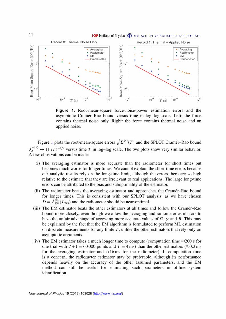
Figure 1. Root-mean-square force-noise-power estimation errors and theasymptotic Cramer–Rao bound versus time in log–log scale. Left: the forcecontains thermal noise only. Right: the force contains thermal noise and anapplied noise.

Figure 1 plots the root-mean-square errors√6(n)l (T ) and the SPLOT Cramer–Rao bound

J −1/2A → (0J T )−1/2 versus time T in log–log scale. The two plots show very similar behavior.

A few observations can be made:

(i) The averaging estimator is more accurate than the radiometer for short times butbecomes much worse for longer times. We cannot explain the short-time errors becauseour analytic results rely on the long-time limit, although the errors there are so highrelative to the estimate that they are irrelevant to real applications. The large long-timeerrors can be attributed to the bias and suboptimality of the estimator.

(ii) The radiometer beats the averaging estimator and approaches the Cramer–Rao boundfor longer times. This is consistent with our SPLOT analysis, as we have chosenD = A(0)EM(Tmax) and the radiometer should be near-optimal.

(iii) The EM estimator beats the other estimators at all times and follow the Cramer–Raobound more closely, even though we allow the averaging and radiometer estimators tohave the unfair advantage of accessing more accurate values of �, γ and R. This maybe explained by the fact that the EM algorithm is formulated to perform ML estimationon discrete measurements for any finite T , unlike the other estimators that rely only onasymptotic arguments.

(iv) The EM estimator takes a much longer time to compute (computation time ≈200 s forone trial with J + 1 = 60 000 points and T = 4 ms) than the other estimators (≈0.3 msfor the averaging estimator and ≈16 ms for the radiometer). If computation timeis a concern, the radiometer estimator may be preferable, although its performancedepends heavily on the accuracy of the other assumed parameters, and the EMmethod can still be useful for estimating such parameters in offline systemidentification.

New Journal of Physics 15 (2013) 103028 (http://www.njp.org/)

12

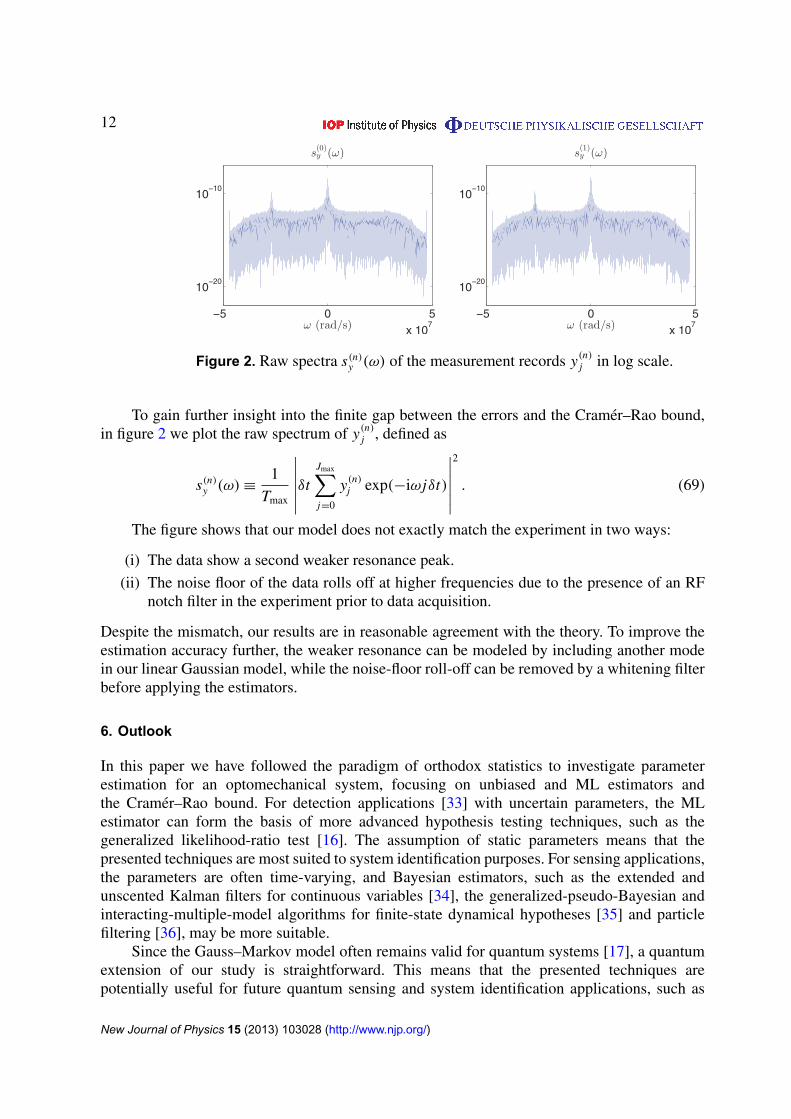
Figure 2. Raw spectra s(n)y (ω) of the measurement records y(n)j in log scale.

To gain further insight into the finite gap between the errors and the Cramer–Rao bound,in figure 2 we plot the raw spectrum of y(n)j , defined as

s(n)y (ω)≡1

Tmax

∣∣∣∣∣∣δtJmax∑j=0

y(n)j exp(−iω jδt)

∣∣∣∣∣∣2

. (69)

The figure shows that our model does not exactly match the experiment in two ways:

(i) The data show a second weaker resonance peak.

(ii) The noise floor of the data rolls off at higher frequencies due to the presence of an RFnotch filter in the experiment prior to data acquisition.

Despite the mismatch, our results are in reasonable agreement with the theory. To improve theestimation accuracy further, the weaker resonance can be modeled by including another modein our linear Gaussian model, while the noise-floor roll-off can be removed by a whitening filterbefore applying the estimators.

6. Outlook

In this paper we have followed the paradigm of orthodox statistics to investigate parameterestimation for an optomechanical system, focusing on unbiased and ML estimators andthe Cramer–Rao bound. For detection applications [33] with uncertain parameters, the MLestimator can form the basis of more advanced hypothesis testing techniques, such as thegeneralized likelihood-ratio test [16]. The assumption of static parameters means that thepresented techniques are most suited to system identification purposes. For sensing applications,the parameters are often time-varying, and Bayesian estimators, such as the extended andunscented Kalman filters for continuous variables [34], the generalized-pseudo-Bayesian andinteracting-multiple-model algorithms for finite-state dynamical hypotheses [35] and particlefiltering [36], may be more suitable.

Since the Gauss–Markov model often remains valid for quantum systems [17], a quantumextension of our study is straightforward. This means that the presented techniques arepotentially useful for future quantum sensing and system identification applications, such as

New Journal of Physics 15 (2013) 103028 (http://www.njp.org/)

13

optomechanical force sensing [18, 20–22], atomic magnetometry [23, 24] and fundamentaltests of quantum mechanics [18, 19, 25]. We expect our parametric methods to lead to moreaccurate quantum sensing and control than robust quantum control methods [23, 37], whichmay be too conservative for the highly controlled environment of typical quantum experiments.There also exist quantum versions of the Cramer–Rao bound that impose fundamental limits tothe parameter estimation accuracy for a quantum system with any measurement [38–40], andit may be interesting to explore how close the classical bounds presented here can get to thequantum limits.

The continued improvement of optomechanical devices for applications and fundamentalscience requires precise engineering of the mechanical resonance frequency, dissipation rateand effective mass. This necessitates a deep understanding of how these mechanical propertiesdepend on differing materials and fabrication techniques. The mechanical resonance frequencyis easily predicted via a numerical eigenmode analysis using the geometry of the structureand the Youngs modulus of the material. It is much more challenging to predict the level ofmechanical dissipation, where numerical models are not as well established and multiple decaychannels usually exist. Effective experimental characterization of such dissipation channelsrequires high precision force estimation to accurately quantify the oscillators coupling to theenvironment. This is critical to advancing optomechanics in applications such as quantummemories and quantum information [41, 42]. A more immediate application for high precisionforce estimation is that of temperature sensing and bolometry where small relative changes ofthe signal power are of interest, for example, in detecting submillimeter wavelengths in radioastronomy [43] or even to search for low energy events in particle physics [44]. Given thedemonstrated success of our statistical techniques, we envision them to be similarly useful forall these applications.

Acknowledgments

SZA and MT acknowledge support by the Singapore National Research Foundationunder NRF grant no. NRF-NRFF2011-07. WPB and GIH acknowledge funding from theAustralian Research Council Centre of Excellence CE110001013 and Discovery ProjectDP0987146. Device fabrication was undertaken within the Queensland Node of the AustralianNanofabrication Facility.

Appendix. EM algorithm for the complex Gauss–Markov model

The model of interest is described by (46)–(49). The parameters of interest, denoted by θ , arethe components of f , c, q and r . Generalizing the algorithm described in [15, 16] for complexvariables, we have

− ln P(Y, Z |θ)=

J−1∑j=0

(z j+1 − f zj

)†q−1

(z j+1 − f zj

)+ J ln det q

+J∑

j=0

(yj − czj

)†r−1

(yj − czj

)+ (J + 1) ln det r +α, (A.1)

New Journal of Physics 15 (2013) 103028 (http://www.njp.org/)

14

where α does not depend on θ and is discarded. To compute the estimated log-likelihoodfunction Q(θ, θ k), we need

zkj ≡ E(zj |Y, θ

k), (A.2)

εkj ≡ zj − zk

j , (A.3)

5kj ≡ E(εk

j εk†j |Y, θ k), (A.4)

5kj, j−1 ≡ E(εk

j εk†j−1|Y, θ

k), (A.5)

which can be computed by the Rauch–Tung–Striebel (RTS) smoother [16, 34]. Starting withstationary initial conditions for z+k

−1 and5+k−1, the smoother consists of a forward Kalman filter:

z−kj = f k z+k

j−1, (A.6)

5−kj = f k5+k

j−1 f k† + q, (A.7)

K +kj =5−k

j ck†(ck5−k

j ck† + r k)−1

, (A.8)

z+kj = z−k

j + K +kj

(yj − ck z−k

j

), (A.9)

5+kj =

(I − K +k

j ck)5−k

j

(I − K +k

j ck)†

+ K +kj r k K +k†

j , (A.10)

until j = J , and a backward propagation:

zkj = z+k

j , (A.11)

5kj = π+k

j , (A.12)

K kj =5+k

j f k†(5−k

j+1

)−1, (A.13)

zkj = z+k

j + K kj

(zk

j+1 − z−kj+1

), (A.14)

5kj = π+k

j − K kj

(5−k

j+1 −5kj+1

)K k†

j , (A.15)

5kj, j−1 =5k

j K k†j−1, (A.16)

until j = 0. We can then write Q(θ, θ k) as

−Q(θ, θ k)= tr{q−1(8k

− f9k†−9k f † + f2k f †

)+ J ln q

+ r−1(ϒ − c4k†

−4kc† + c1kc†)

+ (J + 1) ln r}, (A.17)

where we have defined

8k≡

J∑j=1

(zkj zk†

j +5kj ), (A.18)

9k≡

J∑j=1

(zkj zk†

j−1 +5kj, j−1), (A.19)

New Journal of Physics 15 (2013) 103028 (http://www.njp.org/)

15

2k≡

J−1∑j=0

(zkj zk†

j +5kj ), (A.20)

ϒ ≡

J∑j=0

yj y†j , (A.21)

4k≡

J∑j=0

yj zk†j , (A.22)

1k≡

J∑j=0

(zkj zk†

j +5kj ). (A.23)

Maximizing Q(θ, θ k) with respect to θ , we find

f k+1= ψ k

(2k

)−1, (A.24)

ck+1=4k

(1k

)−1, (A.25)

qk+1=

1

J[8k

−9k(2k)−19k†], (A.26)

r k+1=

1

J + 1[ϒ −4k(1k)−14k†]. (A.27)

One can simply take the real part of equation (A.25) if c is known to be real. The complex EMalgorithm turns out to be the same as the real version with all transpose operations > replacedby conjugate transpose †.

The same algorithm is also applicable to the quantum Gauss–Markov model [17], as theRTS smoother is equivalent to the linear quantum smoother [24, 45, 46]. The possibility ofusing the EM algorithm for quantum systems is also mentioned in [47]. The complex model ismore compact when the noises are phase-insensitive. With phase-sensitive noises, there is nocomputational advantage with a complex model and one can just use a real model to describethe real and imaginary parts separately.

References

[1] Rugar D, Budakian R, Mamin H J and Chui B W 2004 Single spin detection by magnetic resonance forcemicroscopy Nature 430 329–32

[2] Cleland A N and Roukes M L 1998 A nanometre-scale mechanical electrometer Nature 392 160–2[3] Krause A G, Winger M, Blasius T D, Lin Q and Painter O 2012 A high-resolution microchip optomechanical

accelerometer Nature Photon. 6 768–72[4] Forstner S, Prams S, Knittel J, van Ooijen E D, Swaim J D, Harris G I, Szorkovszky A, Bowen W P and

Rubinsztein-Dunlop H 2012 Cavity optomechanical magnetometer Phys. Rev. Lett. 108 120801[5] Jensen K, Kim K and Zettl A 2008 An atomic-resolution nanomechanical mass sensor Nature Nanotechnol.

3 533–7[6] Purdy T P, Peterson R W and Regal C A 2013 Observation of radiation pressure shot noise on a macroscopic

object Science 339 801–4

New Journal of Physics 15 (2013) 103028 (http://www.njp.org/)

16

[7] Verhagen E, Deleglise S, Weis S, Schliesser A and Kippenberg T J 2012 Quantum-coherent coupling of amechanical oscillator to an optical cavity mode Nature 482 63–7

[8] Mancini S, Vitali D and Tombesi P 2003 Scheme for teleportation of quantum states onto a mechanicalresonator Phys. Rev. Lett. 90 137901

[9] Brooks D W C, Botter T, Schreppler S, Purdy T P, Brahms N and Stamper-Kurn D M 2012 Non-classicallight generated by quantum-noise-driven cavity optomechanics Nature 488 476–80

[10] Purdy T P, Yu P-L, Peterson R W, Kampel N S and Regal C A 2013 Strong optomechanical squeezing of lightPhys. Rev. X 3 031012

[11] Safavi-Naeini A H, Groblacher S, Hill J T , Chan J, Aspelmeyer M and Painter O 2013 Squeezed light froma silicon micromechanical resonator Nature 500 185–9

[12] Gavartin E, Verlot P and Kippenberg T J 2012 A hybrid on-chip optomechanical transducer for ultrasensitiveforce measurements Nature Nanotechnol. 7 509–14

[13] Harris G I, McAuslan D L, Stace T M, Doherty A C and Bowen W P 2013 Minimum requirements forfeedback enhanced force sensing Phys. Rev. Lett. 111 103603

[14] Dempster A P, Laird N M and Rubin D B 1977 Maximum likelihood from incomplete data via the EMalgorithm J. R. Stat. Soc. B 39 1–38

[15] Shumway R H and Stoffer D S 2006 Time Series Analysis and its Applications (New York: Springer)[16] Levy B C 2008 Principles of Signal Detection and Parameter Estimation (New York: Springer)[17] Wiseman H M and Milburn G J 2010 Quantum Measurement and Control (Cambridge: Cambridge University

Press)[18] Chen Y 2013 Macroscopic quantum mechanics: theory and experimental concepts of optomechanics J. Phys.

B: At. Mol. Opt. Phys. 46 104001[19] Aspelmeyer M, Kippenberg T J and Marquardt F 2013 Cavity optomechanics arXiv:1303.0733[20] Wheatley T A, Berry D W, Yonezawa H, Nakane D, Arao H, Pope D T, Ralph T C, Wiseman H M, Furusawa A

and Huntington E H 2010 Adaptive optical phase estimation using time-symmetric quantum smoothingPhys. Rev. Lett. 104 093601

[21] Yonezawa H et al 2012 Quantum-enhanced optical-phase tracking Science 337 1514–7[22] Iwasawa K, Makino K, Yonezawa H, Tsang M, Davidovic A, Huntington E and Furusawa A 2013 Quantum-

limited mirror-motion estimation arXiv:1305.0066[23] Stockton J K, Geremia J M, Doherty A C and Mabuchi H 2004 Robust quantum parameter estimation:

coherent magnetometry with feedback Phys. Rev. A 69 032109[24] Petersen V and Mølmer K 2006 Estimation of fluctuating magnetic fields by an atomic magnetometer Phys.

Rev. A 74 043802[25] Tsang M 2013 Testing quantum mechanics arXiv:1306.2699[26] Chow J H, Taylor M A, Lam T T Y, Knittel J, Sawtell-Rickson J D, Shaddock D A, Gray M B, McClelland D E

and Bowen W P 2012 Critical coupling control of a microresonator by laser amplitude modulation Opt.Express 20 12622–30

[27] Lee K H, McRae T G, Harris G I, Knittel J and Bowen W P 2010 Cooling and control of a cavityoptoelectromechanical system Phys. Rev. Lett. 104 123604

[28] Schliesser A, Anetsberger G, Riviere R, Arcizet O and Kippenberg T J 2008 High-sensitivity monitoring ofmicromechanical vibration using optical whispering gallery mode resonators New J. Phys. 10 095015

[29] Van Trees H L 1971 Detection, Estimation and Modulation Theory: III. Radar–Sonar Signal Processing andGaussian Signals in Noise (New York: Wiley)

[30] Van Trees H L 1968 Detection, Estimation and Modulation Theory: I (New York: Wiley)[31] Kailath T 1967 The divergence and Bhattacharyya distance measures in signal selection IEEE Trans.

Commun. Technol. 15 52–60[32] Guta M and Yamamoto N 2013 Systems identification for passive linear quantum systems: the transfer

function approach arXiv:1303.3771

New Journal of Physics 15 (2013) 103028 (http://www.njp.org/)

17

[33] Ting M, Hero A O, Rugar D, Yip C-Yu and Fessler J A 2006 Near-optimal signal detection for finite-statemarkov signals with application to magnetic resonance force microscopy IEEE Trans. Signal Process.54 2049–62

[34] Simon D 2006 Optimal State Estimation: Kalman, H Infinity and Nonlinear Approaches (Hoboken, NJ:Wiley)

[35] Bar-Shalom Y, Li R and Kirubarajan T 2001 Estimation with Applications to Tracking and Navigation (NewYork: Wiley)

[36] Ristic B, Arulampalm S and Gordon N 2004 Beyond the Kalman Filter: Particle Filters for TrackingApplications (Boston, MA: Artech House)

[37] James M R, Nurdin H I and Petersen I R 2008 H∞ control of linear quantum stochastic systems IEEE Trans.Autom. Control 53 1787–803

[38] Helstrom C W 1976 Quantum Detection and Estimation Theory (New York: Academic)[39] Tsang M, Wiseman H M and Caves C M 2011 Fundamental quantum limit to waveform estimation Phys.

Rev. Lett. 106 090401[40] Tsang M 2013 Quantum metrology with open dynamical systems New J. Phys. 15 073005[41] Bagheri M, Poot M, Li M, Pernice W P H and Tang H X 2011 Dynamic manipulation of nanomechanical

resonators in the high-amplitude regime and non-volatile mechanical memory operation NatureNanotechnol. 6 726–32

[42] Rabl P, Kolkowitz S J, Koppens F H L, Harris J G E, Zoller P and Lukin M D 2010 A quantum spin transducerbased on nanoelectromechanical resonator arrays Nature Phys. 6 602–8

[43] Griffin M J 2000 Bolometers for far-infrared and submillimetre astronomy Nucl. Instrum. Methods A444 397–403

[44] Alessandrello A et al 1998 A scintillating bolometer for experiments on double beta decay Phys. Lett. B420 109–13

[45] Tsang M 2009 Time-symmetric quantum theory of smoothing Phys. Rev. Lett. 102 250403[46] Tsang M 2009 Optimal waveform estimation for classical and quantum systems via time-symmetric

smoothing Phys. Rev. A 80 033840[47] Gammelmark S, Julsgaard B and Mølmer K 2013 Past quantum states May 2013, arXiv:1305.0681

New Journal of Physics 15 (2013) 103028 (http://www.njp.org/)