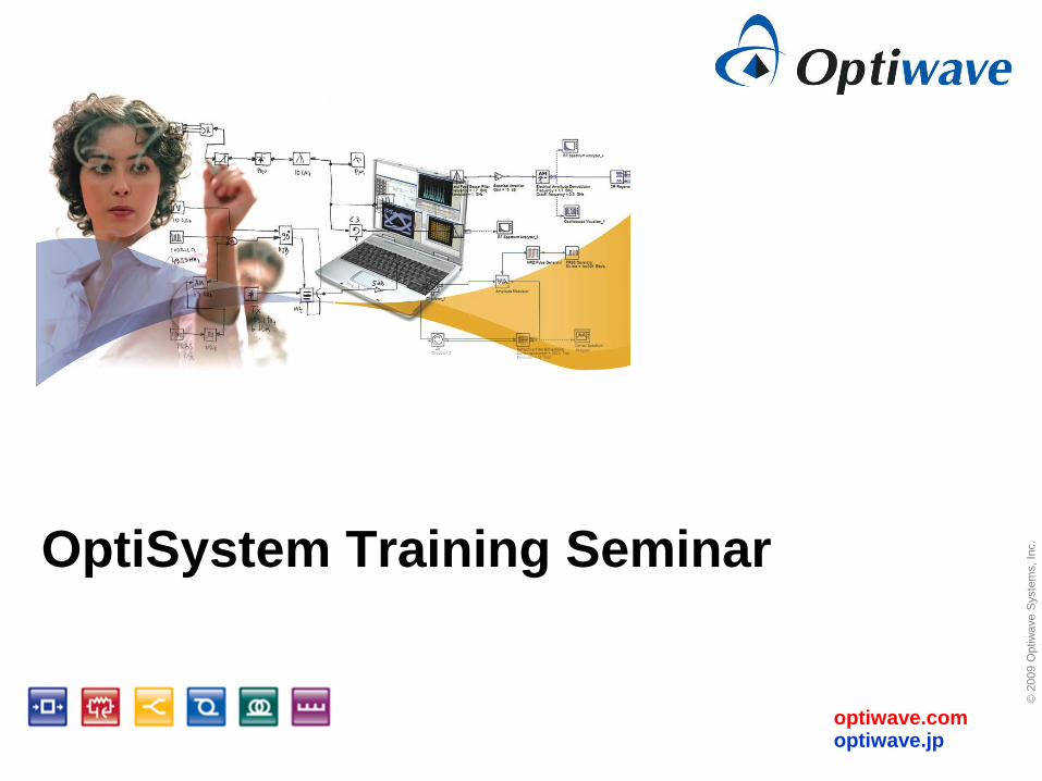
optiwave.com optiwave.jp

© 2

009 O

ptiw

ave S

yste

ms, In

c. OptiSystem Training Seminar

2 2

About Optiwave Systems

Leader in the development of innovative

software tools in Optics

Design, simulation, and optimization of

components, links, systems and networks for

Photonics Nanotechnology, Optoelectronics,

Optical Networks

Established in 1994

Licensed in 1000 industry-leading corporations

and universities in over 60 countries

3 3

Photonics design portfolio

Based on the Beam Propagation Method (BPM), simulates light field

distribution through any waveguide medium

Using an array of mode solvers; calculates dispersion, material losses,

birefringence, and PMD to aid in optimizing parameter selection for single

and multi-mode fiber designs

Based on Coupled Mode theory and the Transfer Matrix method,

simulates the design of waveguide and fiber based periodic structures

Unique circuit design software that incorporates equations governing

optical elements into an electrical simulation framework to provide self-

consistent analysis of opto-electronic circuits

Time and frequency domain simulators for the design of the physical or

transmission layer of optical systems, subsystems and components.

Based on FDTD and UPML boundary condition, solves the E & H fields in

both the spatial and temporal domains, for advanced passive and non-

linear photonic component design

Component design

System design

4 4

About OptiSystem OptiSystem is a time/frequency domain simulator for optical system design.

Applications include:

Optical network design (OTDM, SONET/SDH rings, CWDM, DWDM, PON, Cable, OCDMA)

Single-mode/multi-mode transmission

Free space optics (FSO), Radio over fiber (ROF), OFDM (direct, coherent)

Amplifiers and lasers (EDFA, SOA, Raman, Hybrid, GFF optimization, Fiber Lasers)

Signal processing (Electrical, Digital, All-Optical), Direct/Coherent Tx/Rx design

Modulation formats (RZ, NRZ, CSRZ, DB, DPSK, QPSK, DP-QPSK, PM-QPSK, etc.)

System performance analysis (Eye Diagram/Q-factor/BER, Signal power/OSNR, Polarization

states, Constellation diagrams, Linear and non-linear penalties)

• Default

component

library

• Customized

components

• Co-simulation

components

System & Sub-system

design layouts

Signal representation &

hierarchy between components,

sub-systems, etc.:

• Binary

• Multilevel

• Electrical

• Optical

• Any type

optiwave.com optiwave.jp

© 2

009 O

ptiw

ave S

yste

ms, In

c.

OptiSystem Seminar Module 1: Overview of OptiSystem GUI

features

6 6

Module 1

OptiSystem GUI Overview

Menu/tool bars

Display properties

Project layout

Project browser

Design & analysis tools

Components overview

Application examples

Resources

7 7

OptiSystem GUI: Overview • Default component library

• Custom

• Favorites

• Recently Used

Component inventory/data for

all layouts associated with a

Project Projects tab

Layout Editor

Component

library

Project

Browser

Tool bars Description

docker

Layout tab(s)

Pan window

Scaled view of layout

8 8

OptiSystem GUI: Component library

Default library 400+ components (16 libraries)

Search for components via

“Find component” or “Browse”

features

Custom Create user-defined

components and sub-systems

Favorites Add most often used

components

Recently used Display most recently used

components (up to 10)

9 9

OptiSystem GUI: Menu/Tool bar functions (1)

New project

Open

project

Save

current

project

Print current

project

Cut,

copy,

paste

Undo,

Redo

Calculate

Calculate

Visualizers

Add, Duplicate

layouts

Layout

menu bar

Delete

current

layout

Set total sweep

iterations

Set current

iteration

Previous. Next

sweep iterations

Parameter

sweeps

Layout size,

parameters and

properties

Component, Project

and Description

dockers

Run script

Generate

script

Save

script

Load

script Find

script

Performer

settings

Export

Performer

10 10

OptiSystem GUI: Menu/Tool bar functions(2)

Layout tool

Monitor tool

Draw

output port

Draw rectangle

Draw path

Auto-connect on drop

Draw input

port

Draw circle

Draw line

Draw text label

Bit map tool

Zoom in

Zoom out

Zoom to

window

Zoom 1:1

Auto-connect on move

View component parameters

View port signal data

View component results

11 11

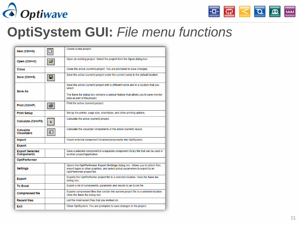
OptiSystem GUI: File menu functions

12 12

OptiSystem GUI: Edit menu functions (1)

Layout tools. Also available

via menu bars

Component tools. Also

available via project layout

context tool

13 13

OptiSystem GUI: Edit menu functions (2)

Also available via project

layout context tool

14 14

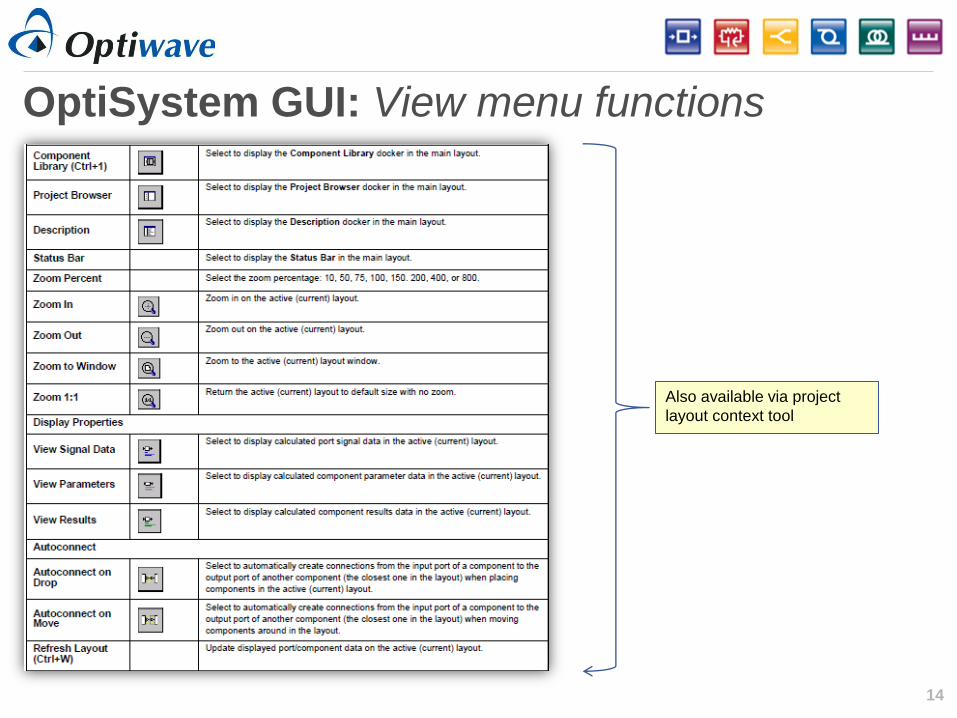
OptiSystem GUI: View menu functions

Also available via project

layout context tool

15 15

OptiSystem GUI: Layout menu functions

Also available via project

layout context tool

16 16

OptiSystem GUI: Tools/Report/Help menu

Use this function (or the

shortcut) to add new report

pages

Provides access to html help

version of the User

Reference guide

Also accessed via the

Calculations dialog box

17 17

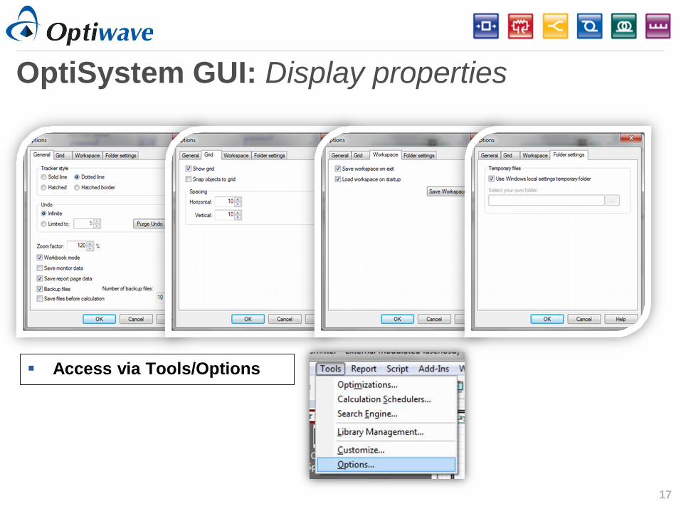
OptiSystem GUI: Display properties

Access via Tools/Options

18 18

Project layout: Layout properties

Name, author and date is reflected within

the Layout properties header

19 19

Project layout: Accessing/modifying components

• View or modify all parameters linked to

a component

• Enable or disable for simulation

• Access results (when available)

following a calculation

• Create a VB script that is specific to

the component

20 20

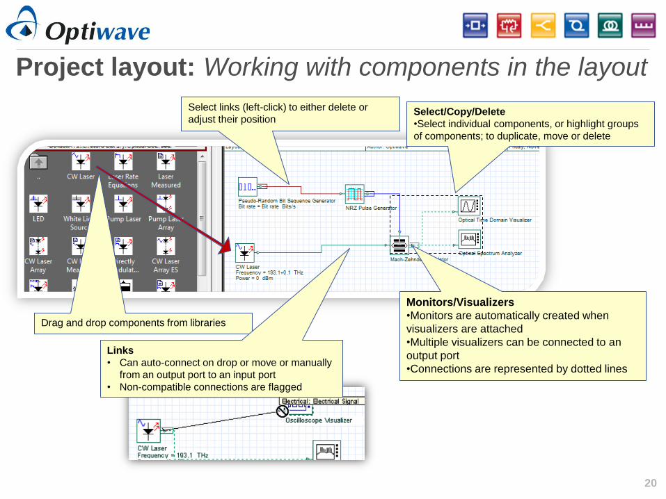
Project layout: Working with components in the layout

Drag and drop components from libraries

Select/Copy/Delete

•Select individual components, or highlight groups

of components; to duplicate, move or delete

Select links (left-click) to either delete or

adjust their position

Links

• Can auto-connect on drop or move or manually

from an output port to an input port

• Non-compatible connections are flagged

Monitors/Visualizers

•Monitors are automatically created when

visualizers are attached

•Multiple visualizers can be connected to an

output port

•Connections are represented by dotted lines

21 21

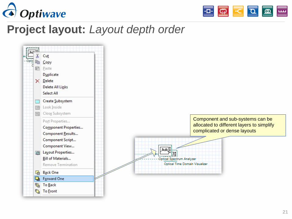
Project layout: Layout depth order

Component and sub-systems can be

allocated to different layers to simplify

complicated or dense layouts

22 22

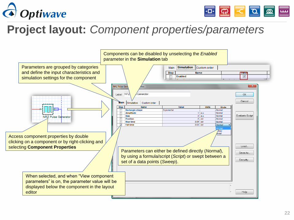
Project layout: Component properties/parameters

Parameters can either be defined directly (Normal),

by using a formula/script (Script) or swept between a

set of a data points (Sweep).

Parameters are grouped by categories

and define the input characteristics and

simulation settings for the component

Access component properties by double

clicking on a component or by right-clicking and

selecting Component Properties

Components can be disabled by unselecting the Enabled

parameter in the Simulation tab

When selected, and when “View component

parameters” is on, the parameter value will be

displayed below the component in the layout

editor

23 23

Project layout: Visualizers properties/parameters

Access visualizers by right clicking and

selecting Component Properties

Parameters used to defined measurement and

graph settings

24 24

Project layout: Port properties

Label information and port

position/location can only be modified for

sub-systems

Determine which signal data to view

when “View port signal data” is

activated.

Hover mouse over port (and right-click) to

access Port Properties

25 25

Project layout: Data monitors & signal tracing

Data monitors Data passed through ports can have large amounts of data (this data is saved only at ports where

monitors are present)

It is important to keep monitors to a minimum to reduce memory requirements!

Select monitor tool and hover over output ports that

you wish to add or remove data monitors

Port data appears (after calculation) when

“View Port Signal data” is selected

Note: Calculate signal tracing must also be

enabled in Global Parameters

26 26

Project layout: Adding objects and text

Double click on objects to

modify line and fill colors

Create text boxes and edit text type, font

and colour

Add images (bit map, jpeg)

to the layout

Basic tools: Lines,

rectangles, circles/ellipses

27 27

Project layout: Bill of Materials

Defined in the Custom order tab

for Component properties

28 28

Project browser: Overview

Lists all information for a project The components in the project layout are synchronized with those in the project browser view

(when you click a component in the project browser, the same component is selected in the

layout (and vice versa))

All information linked to any component (or the layout) can be viewed through an expandable

menu tree structure

Global layout settings including Global

parameters, Sweeps and Paths

Data on each component includes:

• Ports

• Parameters

• Results (when applicable)

• Graphs (when applicable)

29 29

Project browser: View settings

Create and access customized views

30 30

Design and analysis tools: Visualizers

Optical / RF Spectrum Analyzer

Resolution filter, Signal analysis

Oscilloscope

Amplitude, Power, Chirp

EYE Diagram Analyzer

Masks and Histograms

BER Analyzer

Numerical and quasi-analytical analysis

WDM Analyzer

Calculate power, wavelengths, S/N ratios

Signal Analyzer

Statistical analysis

31 31

Design and analysis tools: Path tool

32 32

Design and analysis tools: Graphs

The graphic icons (2D/3D) appear for all graphs that can be viewed

Double-click, or right click and select Quick view, to preview the graph results

The Component view feature can also be used to visualize 2D and 3D graphs

33 33

Design and analysis tools: Results

Displays values representing calculated data generated by a component

Cab be accessed via Project browser, Component view and Component Results

Checked values will be

displayed in the project

layout (just below the

component) If a calculated value is

outside the min-max points,

it will be displayed in a red

font

34 34

Design and analysis tools: Reports

Create

Tables

2D Graphs

3D Graphs

Plot parameters vs.

results

35 35

Design and analysis tools: Scripts

Uses standard VB script

language.

Allows changes in the

parameters of current

project.

Can be used for post-

processing of

simulation results.

36 36

Design and analysis tools: Optimizations

Single-parameter optimization

Multiple-parameter optimization

GFF optimization

Monte Carlo Yield Estimate

37 37

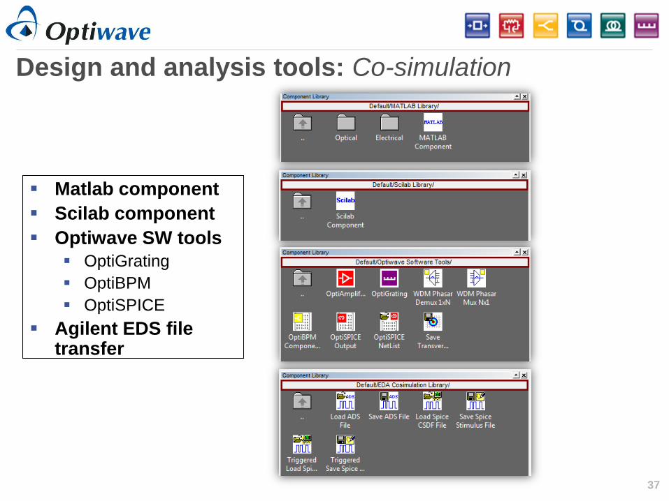
Design and analysis tools: Co-simulation

Matlab component

Scilab component

Optiwave SW tools

OptiGrating

OptiBPM

OptiSPICE

Agilent EDS file transfer

38 38

Components overview

39

Application examples

40

Digital Link Design Using Different Modulation Formats RZ, NRZ

Duobinary

CSRZ

DPSK

DQPSK 100 km 165 km 180 km

41

WDM Systems

DWDM

CWDM

42

Multimode Link

43

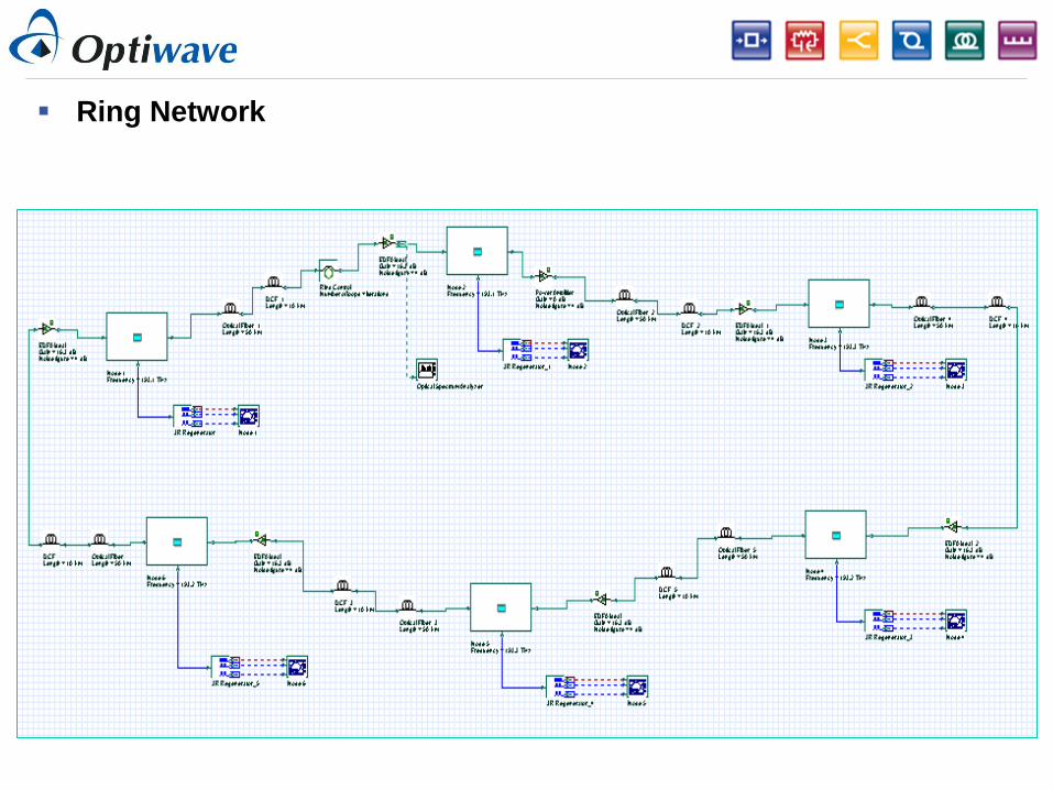
Ring Network

44

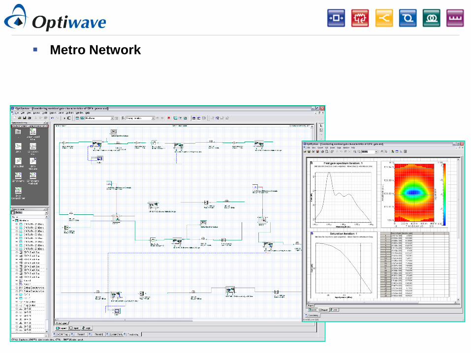
Metro Network

45

CATV Systems

46

Optical Amplifier Design

EDFA

YDFA

EYDFA

RFA

47 47

PON-Bidirectional Transmission

48 48

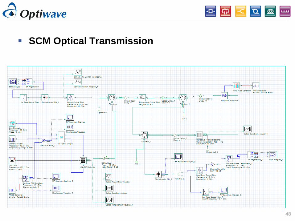
SCM Optical Transmission

49 49

Resources (1)

Documentation OptiSystem Component Library

OptiSystem Getting Started

OptiSystem Tutorials Vol 1 & Vol 2

OptiSystem User Reference

OptiSystem VBScripting Ref Guide

Component help

50 50

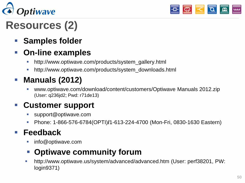
Resources (2)

Samples folder

On-line examples http://www.optiwave.com/products/system_gallery.html

http://www.optiwave.com/products/system_downloads.html

Manuals (2012) www.optiwave.com/download/content/customers/Optiwave Manuals 2012.zip

(User: q236jd2; Pwd: r71de13)

Customer support support@optiwave.com

Phone: 1-866-576-6784(OPTI)/1-613-224-4700 (Mon-Fri, 0830-1630 Eastern)

Feedback info@optiwave.com

Optiwave community forum http://www.optiwave.us/system/advanced/advanced.htm (User: perf38201, PW:

login9371)

optiwave.com optiwave.jp

© 2

009 O

ptiw

ave S

yste

ms, In

c. OptiSystem Seminar

Module 2: System design

52 52

Module 2 (1) Signals

Global parameters

Calculate tab overview

Project 1: Transmitter – External modulated laser Project layout

Component parameters

Visualizers

Info-window features

Project 2: Subsystems — Hierarchical simulation Creating a sub-system with ports

Subsystem properties

Accessing global parameters

Adding a custom component to the library

53 53

Module 2 (2) Project 3: Optical Systems — WDM Designs

Parameter groups

Fiber/EDFA spans

BER Analysis

3D graphs

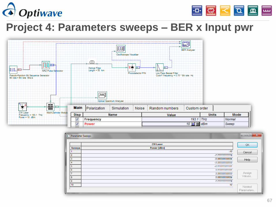
Project 4: Parameter Sweeps — BER x Input

power Setting up sweep iterations

Browsing iteration results

Analyzing results with Reports

54 54

Signals: Types & representation

Binary Sequences of 1’s & 0’s

Created by bit sequence

generators

M-ary Multi-level discrete values for

advanced modulation (PAM, QAM,

QPSK)

Electrical Generated by electrical pulse

generators and photo-detectors

Sampled in time domain

Optical Generated by optical sources (e.g.

lasers) and optical pulse

generators

Sampled in time domain

55 55

Signals: Electrical

Pulse generators Create noise-less time domain sampled waveform

Photo-detectors On top of time domain sampled waveform may contain information on time variance noise (shot)

or power spectral density (thermal)

Sampled signal waveform

in time domain.

Signal noise variances in

time domain.

Noise power spectral densities

in frequency domain.

56 56

Signals: Optical

Sampled signals (optical sources) Time domain representation of optical signal

Can be represented in independent bands or in the same continuous frequency band

Spatial mode data is also available

Parameterized signals Time-averaged descriptions of sampled signals (Average power, Central frequency, and

Polarization state)

Useful for performing a fast estimation of system performance (power budget, OSNR)

Noise bins Represent optical noise via average spectral density in two polarizations (power spectral density

x bandwidth)

Propagated separately from the optical sampled signals (but can be combined with signals for

overlapping bands

Parameterized Adaptive noise bins

Sampled signals

57 57

Global parameters: Simulation tab • Set bit rate (Default mode)

• Set time window

• Set sample rate

The global Bit rate can affect components such as Bit sequence generators (which may use as

a default value) and the value for the bandwidth or cut-off frequency of most electrical filters.

The Time window affects all components (each component works with the same time window).

This parameter is best expressed in terms of the sequence length and the bit rate used during

the simulation.

The global Sample rate specifies the frequency simulation window or simulation bandwidth in

Hz. It can affect components such as pulse generators and optical sources that generate signals

at different sample rates. It is normally best to operate all modules in the design at the same

sample rate

The Sequence length should be set based on the simulation objectives. Use long sequences

for transmission metrics (such as eye diagrams & BER) and short sequences to study optical

effects (such as pulse dispersion)

When enabled, closest Time

window or Sample rate is found

Set by the user

Set by the user

Always calculated (Sequence

length X Samples/bit)

58 58

The Samples per bit, or the number of samples taken over a bit period (0 or 1), must be a power of

two (2, 4, 8, 16, …). The sampling rate is automatically adjusted after Samples per bit is changed

The Sequence length, the number of bits that are captured within a given time (or sampling)

window in seconds, must also be a power of two.

The Sampling rate is calculated by taking the inverse of the sampling time T (the time interval

between performing measurements on the analog signal). If the highest known or expected

frequency component (non-negligible) of the signal stream is Fsample, then the sampling rate

should be set to at least 2 X Fsample (Nyquist rate) to ensure good fidelity of the reconstructed

signal.

Defines the frequency spacing

in the freq domain.

TW = Seq. length X Bit period

Df = 1/Time window

= Sample rate/# samples Samples per bit

Global parameters: Simulation basics

Time spacing = 1/Sample rate

Time domain samples =

Freq domain samples

59 59

Global parameters: Simulation tab (GPU)

60 60

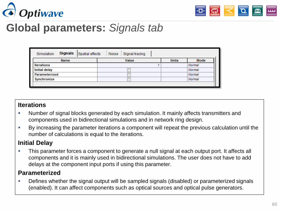
Global parameters: Signals tab

Iterations

Number of signal blocks generated by each simulation. It mainly affects transmitters and

components used in bidirectional simulations and in network ring design.

By increasing the parameter iterations a component will repeat the previous calculation until the

number of calculations is equal to the iterations.

Initial Delay

This parameter forces a component to generate a null signal at each output port. It affects all

components and it is mainly used in bidirectional simulations. The user does not have to add

delays at the component input ports if using this parameter.

Parameterized

Defines whether the signal output will be sampled signals (disabled) or parameterized signals

(enabled). It can affect components such as optical sources and optical pulse generators.

61 61

Global parameters: Spatial effects tab

The spatial effects parameters affect components that generate spatial modes, where the

discretization space and the level of the discretization should be defined.

The number of points per spatial mode is defined as the product of the number of points in the X

and Y

62 62

Global parameters: Signal tracing tab

OptiSystem allows for fast estimation of power and noise at each output port. This

estimation is calculated every time a signal is sent to the component output port.

The signal tracing parameters allow the user to control the calculation and

presentation of the results

Defines if noise floor will be

calculated using interpolation

Hz, m, THZ or nm

dBm, W or mW

63 63

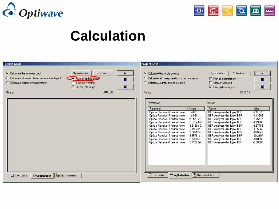
Calculate tab overview

Calculate the whole project

Calculates all the layouts

and all the sweep iterations

within each layout.

Calculate all sweep iterations in

the active layout

Calculates all the sweep

iterations within the current

active layout only.

Calculate current sweep iteration

Calculates only the selected

sweep iteration in the

current layout.

Setup optimizations for layout

Disables & cleans the signal buffers at the

end of the calculation. When disabled,

user can perform large number of sweeps.

Start calculation

Pause calculation

Stop calculation

64 64

Project 1: Transmitter – External modulated laser

65 65

Project 2: Subsystems – hierarchical simulation

OS allows for the creation of

multiple layers of

subsystems. Subsystems are

identical to components

(icons, parameters, ports)

and may comprise a group of

components or other

subsystems.

66 66

Project 3: Optical Systems - WDM design

67 67

Project 4: Parameters sweeps – BER x Input pwr

optiwave.com optiwave.jp

© 2

009 O

ptiw

ave S

yste

ms, In

c. OptiSystem Seminar

Module 3: Advanced topics

69 69

Module 3 Bi-directional simulation

Bidirectional Simulation — Working with multiple iterations

(OptiSystem_Tutorials_Volume_1, pp. 87-96)

Optimization APD gain optimization (single parameter goal attaining)

Scripts

Nested sweeps

70

Optimizations

71 71

Application Example: Receiver

Calibration

Sensitivity: The minimum amount of power required to achieve a specific receiver performance.

Sensitivity: -18 dBm, Bit rate:10 GBs, Modulation: NRZ, log(BER):-10

For a given layout and parameters, optimize receiver noise until the log(BER) is equal to ‘-10’

72

Create System Layout

73

Creating Optimizations

74

Optimization Setup

75

Calculation

76

Results

77 77

More about Optimizations

Cascaded optimizations

Priority levels

Parameter sweep and optimizations

AGC

APC

Gain Flattening Filter/Equalization optimizations

78 78

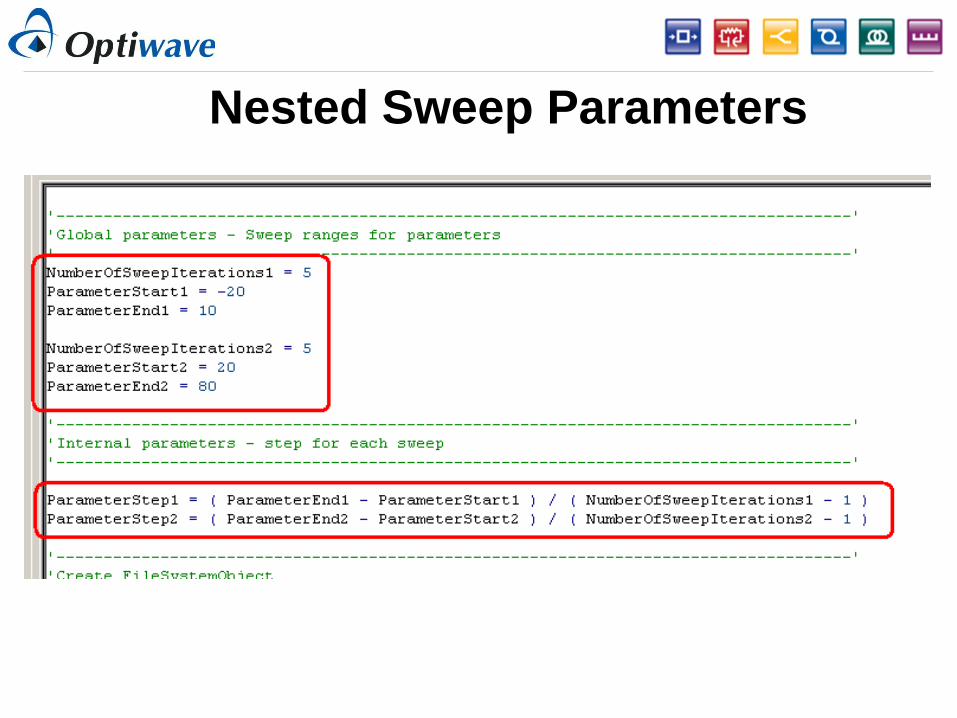
Nested Parameter Sweeps

If you set more than one parameter to sweep

mode, you can create nested parameter

sweeps.

79 79

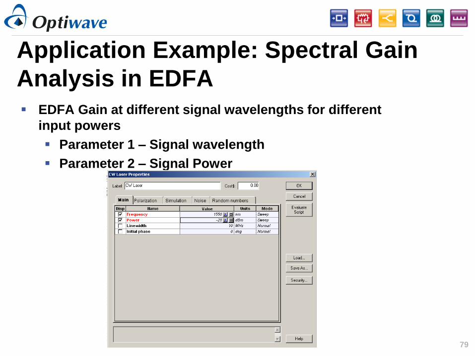
Application Example: Spectral Gain

Analysis in EDFA EDFA Gain at different signal wavelengths for different

input powers

Parameter 1 – Signal wavelength

Parameter 2 – Signal Power

80 80

Sweep Setup

81 81

Sweep Setup

82 82

Sweep Setup

83 83

Combinations for nested parameter

sweeps (Plotting Graphs)

84 84

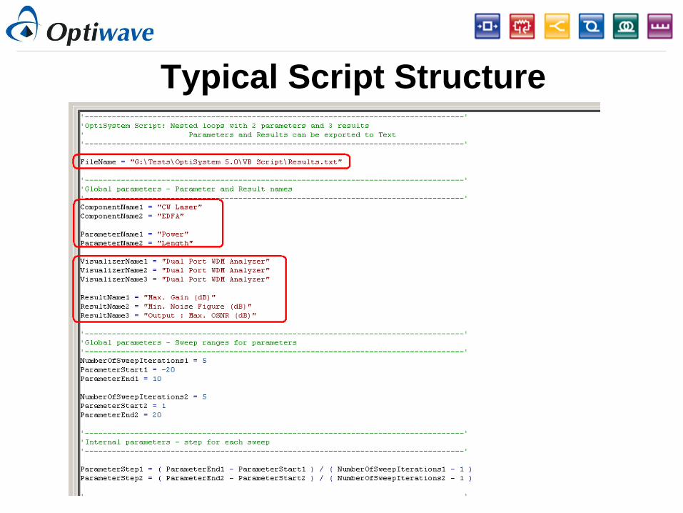
Script Overview

Architecture

Advantages of using script Automation: access to Excel, MATLAB, etc.

Low memory requirements

Customization of calculation

Typical applications Large number of sweeps

Nested sweeps

85

OptiSystem Script

86 86

Setup

Create design

Load script template

Modify template

Run script

Post process results

87

Load or Create Design

88

Load Script Template

89

Typical Script Structure

90

Nested Sweep Parameters

91

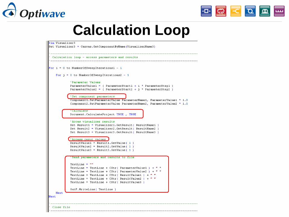
Calculation Loop

92

Run Script and Obtain Results

93 93

Component Script

The script function allows to view or change parameter

values, graphs and results of a selected component.

94 94

Component Script example

Calculates the average population inversion in a

doped fiber amplifier.

Create the population inversion result

Add the script code to calculate the average

population inversion base on the Normalized

population density graph.

95 95

Adding the component result

96 96

Scheduling

1

1

2

3

Signal

97 97

Disconnected Component

1

1 X

X

Signal

98 98

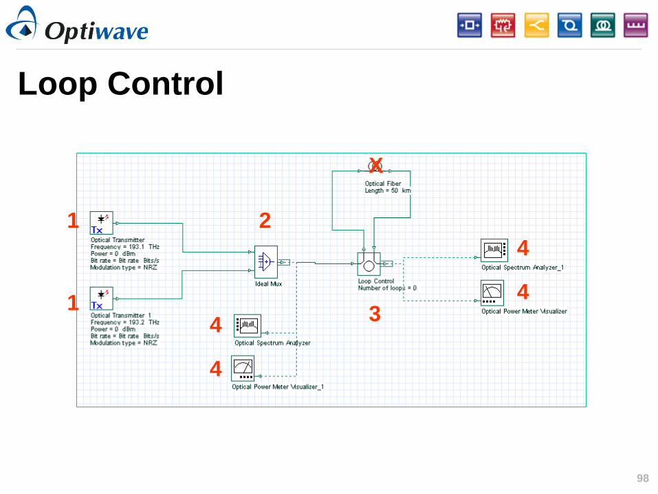
Loop Control

1

1

2

3 4

4

4

4

X

99 99

Loop Control

1

1

2

3 8

8

8

8

4

5

6

7

10

0

Signal Index

Signal

Index = 0

Index = 1

10

1

Disconnected Bidirectional

Components

1

1

X

X

2 X

3

10

2

Bidirectional Components

1

1

3

4

2

4

4

1

10

3

Cascading Components

1

1 X

2 X

1

X

10

4

Cascading Components

1

1

3 2

5

1

4

10

5

Global Parameter: Iterations

Signal

10

6

Bidirectional Simulations

10

7

Bidirectional EDFA (initial delay)

10

8

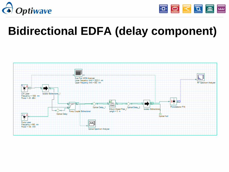
Bidirectional EDFA (delay component)

10

9

Time-Driven simulation

The simulation can convert signals to “Individual Samples”

Individual sample is a signal type that allows the users to

simulate time-driven systems in the electrical and optical

domain.

By using time-driven simulation, users can create designs

that have closed loops and feedbacks.

11

0

Time-Driven simulation

Time driven simulations are slower than comparable, block

mode

Important global parameters are:

Sequence length

Samples per bit

11

1

Individual samples vs sampled signals

This filter operates on

individual samples

This filter operates on

sampled signal

Tool for duplicating any signal

(perfect duplication)

11

2

Gain-clamped EDFA in a ring laser

11

3

113

Unlimited capabilities with

MATLAB

Co-simulation Design and analyze algorithms for the physical layer of

optical communication components and systems

Analysis Data visualization, data analysis, and numerical

computation of OptiSystem results

Optimizations Widely used algorithms for standard and large-scale

optimization.

11

4

114

Matlab code

11

5

115

Unlimited capabilities with

MATLAB

Co-simulation Design and analyze algorithms for the physical layer of

optical communication components and systems

Analysis Data visualization, data analysis, and numerical

computation of OptiSystem results

Optimizations Widely used algorithms for standard and large-scale

optimization.

11

6

116

Analysis

Post-Processing

11

7

117

Matlab code

11

8

118

Simulation Results

11

9

119

Optical Circuits (OptiBPM)

Ring Ressonator

12

0

120

OCDMA System (OptiGrating)

12

1

121

OptiPerformer

It is a free software that can read and simulate encrypted files exported by OptiSystem

Same accuracy of OptiSystem, with a customized interface

Allows users to generate files that can be shared with people who do not have a license of OptiSystem

Users: students, coworkers, marketing and sales teams

12

2

122

OptiPerformer