Options Parity
47
Computational Finance 1/47 Derivative Securities Forwards and Options 381 Computational Finance Imperial College London
-
Upload
sweetypie4u -
Category
Documents
-
view
222 -
download
0
Transcript of Options Parity
8/7/2019 Options Parity
http://slidepdf.com/reader/full/options-parity 1/47
Computational Finance 1/47
Derivative SecuritiesForwards and Options
381 Computational Finance
Imperial College
London
8/7/2019 Options Parity
http://slidepdf.com/reader/full/options-parity 2/47
Computational Finance 2/47
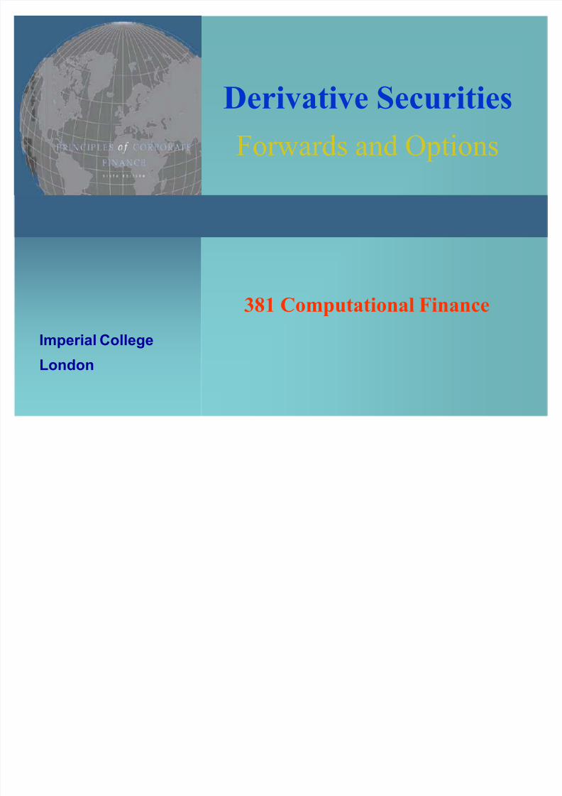
Topics Covered
Derivatives:
Forward Contracts, Options
Valuation techniques
Option Pricing Models
Binomial Option Pricing
8/7/2019 Options Parity
http://slidepdf.com/reader/full/options-parity 3/47
Computational Finance 3/47
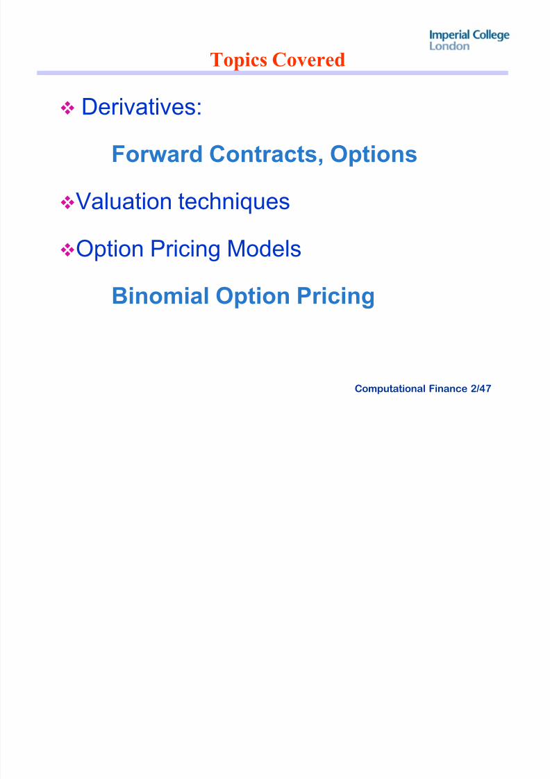
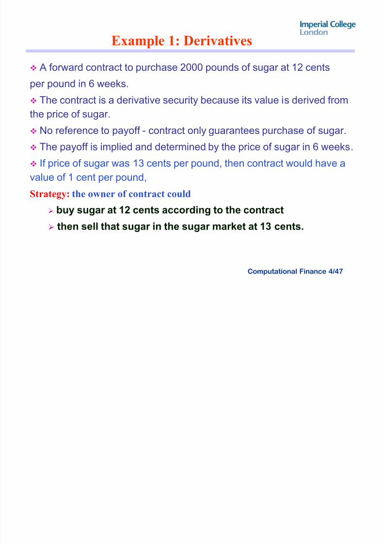
Introduction to Derivatives
securitywhose payoff is explicitly tied to value or price of other financial security
that determines value of derivative is called underlying security
derivatives
arise when individuals or companies wish to buy asset or commodity in
advance to insure against adverse market movements;effective tools for hedging risks ± designed to enable market participants to
eliminate risk.
business dealing with a good faces risk associated with price fluctuations.
control that risk through use of derivative securities.
Example:
farmer can fix price for crop even before planting, eliminating price risk
an exporter can fix a foreign exchange rate even before beginning to
manufacture product, eliminating foreign exchange risk.
8/7/2019 Options Parity
http://slidepdf.com/reader/full/options-parity 4/47
8/7/2019 Options Parity
http://slidepdf.com/reader/full/options-parity 5/47
Computational Finance 5/47
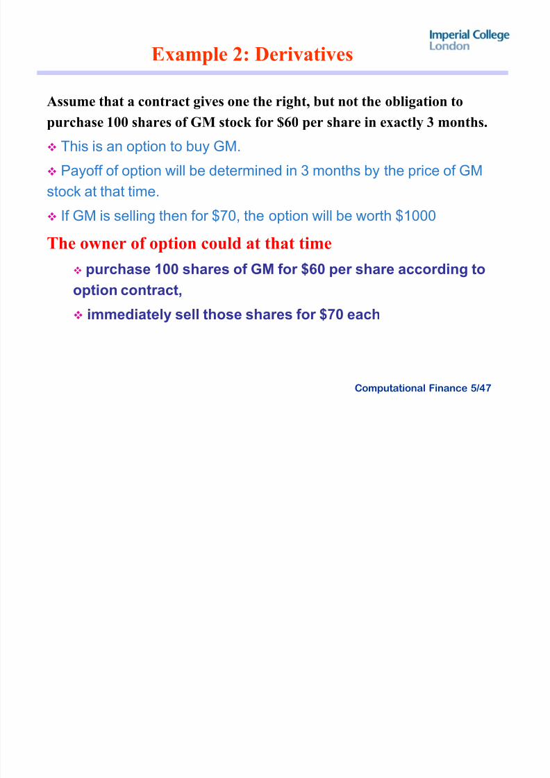
Example 2: Derivatives
Assume that a contract gives one the right, but not the obligation to
purchase 100 shares of GM stock for $60 per share in exactly 3 months.
This is an option to buy GM.
Payoff of option will be determined in 3 months by the price of GM
stock at that time. If GM is selling then for $70, the option will be worth $1000
The owner of option could at that time
purchase 100 shares of GM for $60 per share according to
option contract,
immediately sell those shares for $70 each
8/7/2019 Options Parity
http://slidepdf.com/reader/full/options-parity 6/47
Computational Finance 6/47
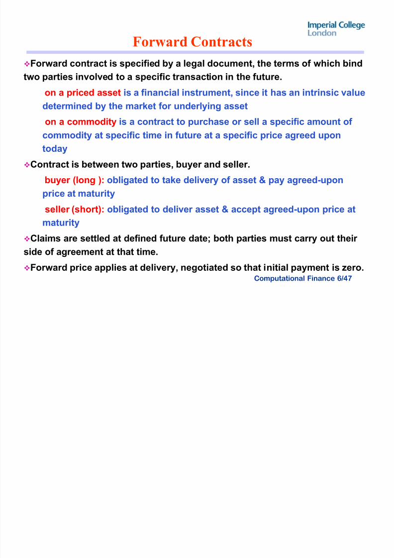
Forward Contracts
Forward contract is specified by a legal document, the terms of which bind
two parties involved to a specific transaction in the future.
on a priced asset is a financial instrument, since it has an intrinsic value
determined by the market for underlying asset
on a commodity is a contract to purchase or sell a specific amount of
commodity at specific time in future at a specific price agreed upontoday
Contract is between two parties, buyer and seller.
buyer (long ): obligated to take delivery of asset & pay agreed-upon
price at maturity
seller (short): obligated to deliver asset & accept agreed-upon price at
maturity
Claims are settled at defined future date; both parties must carry out their
side of agreement at that time.
Forward price applies at delivery, negotiated so that initial payment is zero.
8/7/2019 Options Parity
http://slidepdf.com/reader/full/options-parity 7/47
8/7/2019 Options Parity
http://slidepdf.com/reader/full/options-parity 8/47
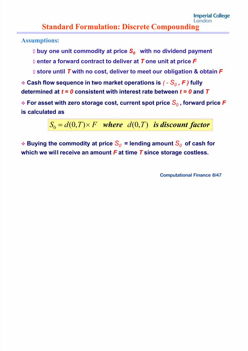
Computational Finance 8/47
Standard Formulation: Discrete Compounding
Assumptions:
buy one unit commodity at price S 0 with no dividend payment
enter a forward contract to deliver at T one unit at price F
store until T with no cost, deliver to meet our obligation & obtain F
Cash flow sequence in two market operations is ( - S 0
, F ) fully
determined at t = 0 consistent with interest rate between t = 0 and T
For asset with zero storage cost, current spot price S 0 , forward price F
is calculated as
Buying the commodity at price S 0 = lending amount S 0 of cash for
which we will receive an amount F at time T since storage costless.
factor discount is where ),0(),0(0
T d F T d S v!
8/7/2019 Options Parity
http://slidepdf.com/reader/full/options-parity 9/47
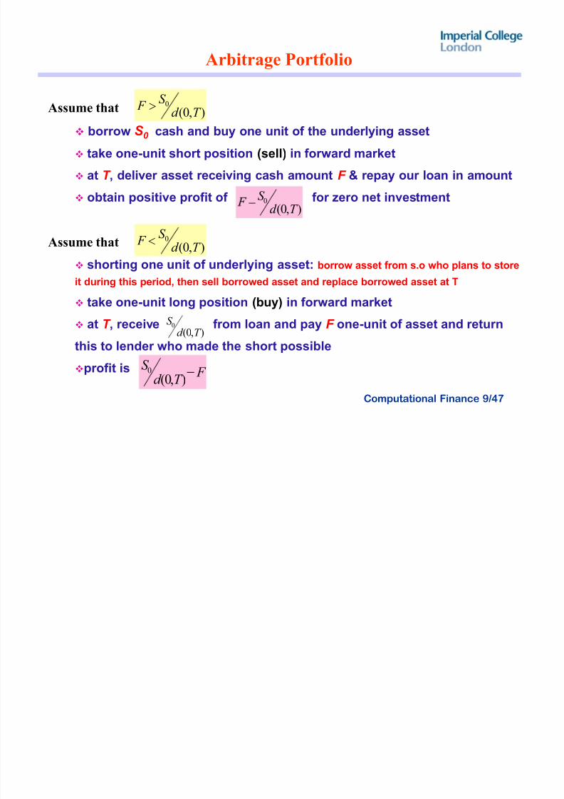
Computational Finance 9/47
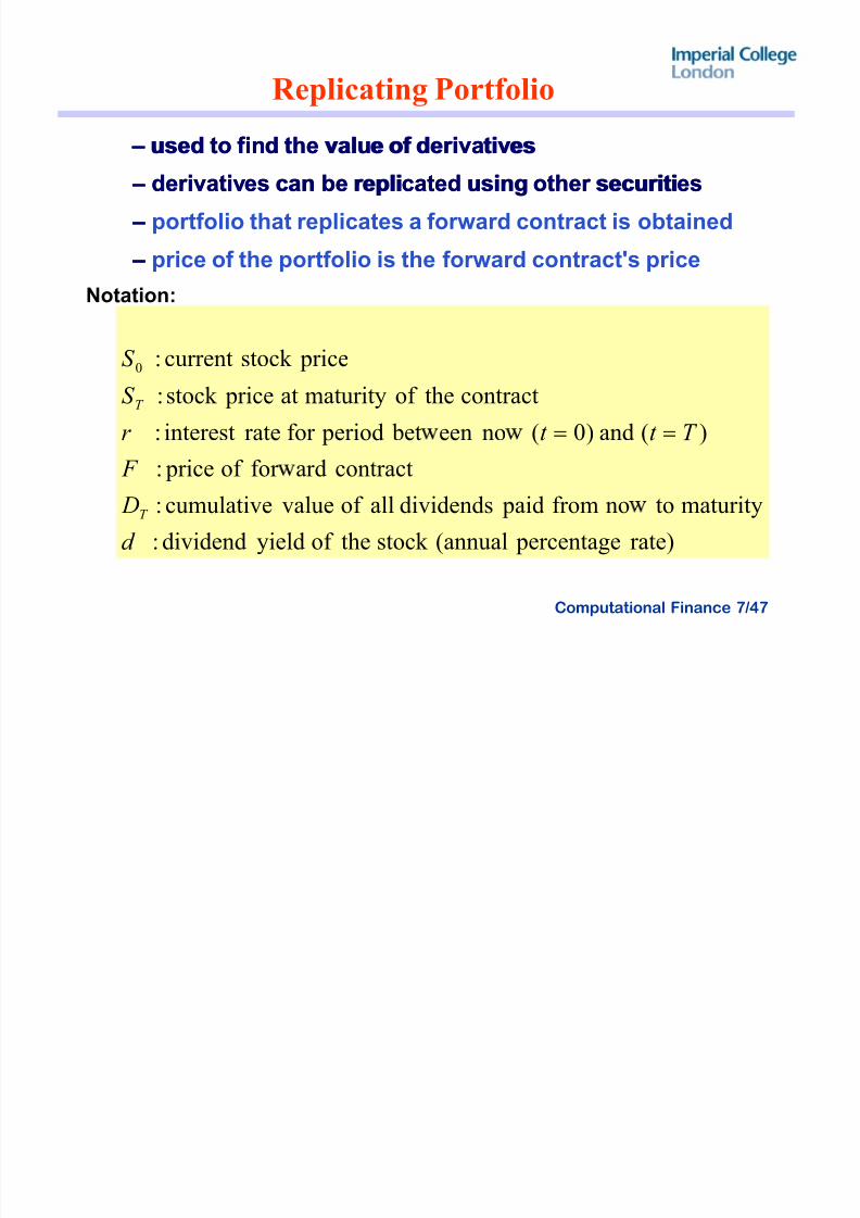
Arbitrage Portfolio
Assume that
borrow S 0 cash and buy one unit of the underlying asset
take one-unit short position (sell) in forward market
at T , deliver asset receiving cash amount F & repay our loan in amount
obtain positive profit of for zero net investment
Assume that
shorting one unit of underlying asset: borrow asset from s.o who plans to store
it during this period, then sell borrowed asset and replace borrowed asset at T
take one-unit long position (buy) in forward market
at T , receive from loan and pay F one-unit of asset and return
this to lender who made the short possible
profit is
),0(0
T d S F "
),0(0
T d S
),0(0
T d S
F
F T d
S ),0(
0
),0(0
T d S
8/7/2019 Options Parity
http://slidepdf.com/reader/full/options-parity 10/47
Computational Finance 10/47
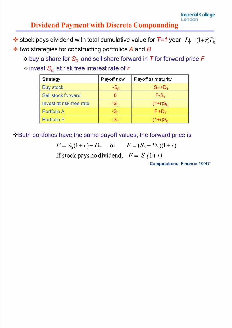
Dividend Payment with Discrete Compounding
stock pays dividend with total cumulative value for T=1 year two strategies for constructing portfolios A and B
¹ buy a share for S 0 and sell share forward in T for forward price F
¹ invest S 0 at risk free interest rate of r
Both portfolios have the same payoff values, the forward price is
Strategy Payoff now Payoff at maturityBuy stock -S0 ST +DT
Sell stock forward 0 F-ST
Invest at risk-free rate -S0 (1+r)S0
Portfolio A -S0 F +DT
PortfolioB
-S0 (1+r)S0
0)1( Dr DT !
r)( S F
r DS F Dr S F T
!
!!
1 dividend,no paysstock If
)1)((or )1(
0
000
8/7/2019 Options Parity
http://slidepdf.com/reader/full/options-parity 11/47
Computational Finance 11/47
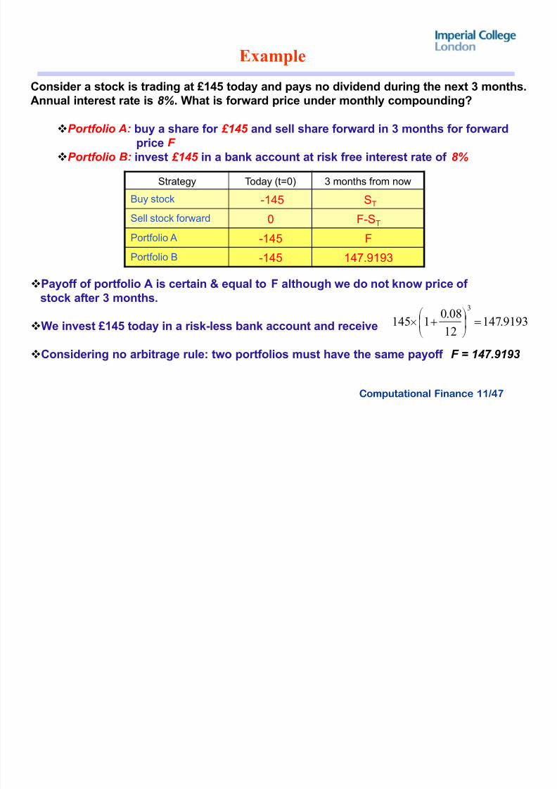
Example
Consider a stock is trading at £145 today and pays no dividend during the next 3 months.
Annual interest rate is 8%. What is forward price under monthly compounding?
Por tf olio A: buy a share for £145 and sell share forward in 3 months for forwardprice F
Por tf olio B: invest £145 in a bank account at risk free interest rate of 8%
Payoff of portfolio A is certain & equal to F although we do not know price of stock after 3 months.
We invest £145 today in a risk-less bank account and receive
Considering no arbitrage rule: two portfolios must have the same payoff F = 147.9193
Strategy Today (t=0) 3 months from now
Buy stock -145 ST
Sell stock forward 0 F-ST
Portfolio A -145 F
Portfolio B -145 147.9193
9193.14712
08.01145
3
!¹ º
¸©ª
¨v
8/7/2019 Options Parity
http://slidepdf.com/reader/full/options-parity 12/47
Computational Finance 12/47
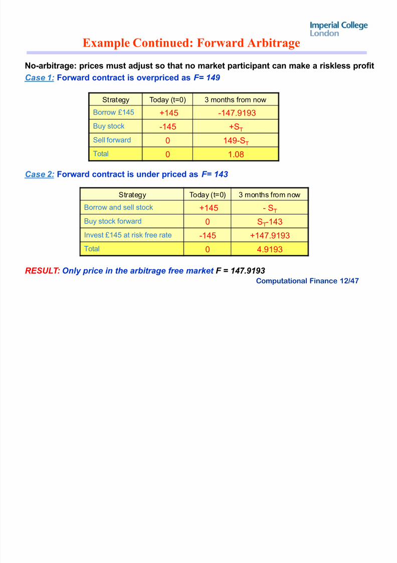
Example Continued: Forward Arbitrage
No-arbitrage: prices must adjust so that no market participant can make a riskless profitCase 1: Forward contract is overpriced as F = 149
Case 2: Forward contract is under priced as F = 143
RE SULT : Only pric e i n the arbi t r age f r ee mark et F = 147.9193
Strategy Today (t=0) 3 months from now
Borrow £145 +145 -147.9193
Buy stock -145 +ST
Sell forward 0 149-ST
Total 0 1.08
Strategy Today (t=0) 3 months from now
Borrow and sell stock +145 - ST
Buy stock forward 0 ST-143
Invest £145 at risk free rate -145 +147.9193
Total 0 4.9193
8/7/2019 Options Parity
http://slidepdf.com/reader/full/options-parity 13/47
Computational Finance 13/47
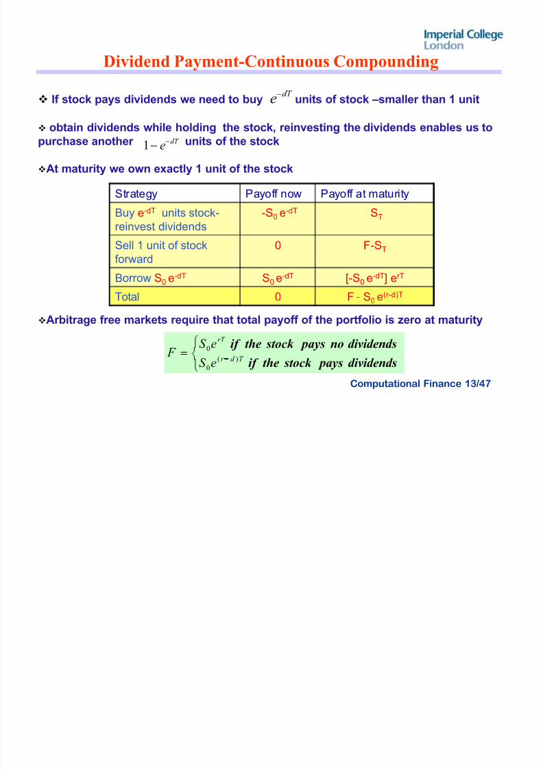
Dividend Payment-Continuous Compounding
If stock pays dividends we need to buy units of stock ±smaller than 1 unit
obtain dividends while holding the stock, reinvesting the dividends enables us topurchase another units of the stock
At maturity we own exactly 1 unit of the stock
Arbitrage free markets require that total payoff of the portfolio is zero at maturity
Strategy Payoff now Payoff at maturity
Buy e-dT units stock-reinvest dividends
-S0 e-dT ST
Sell 1 unit of stockforward
0 F-ST
Borrow S0e-dT S
0e-dT [-S
0e-dT] erT
Total 0 F - S0 e(r-d)T
°¯®
!dividends paysstock theif
dividendsno paysstock theif T d r
rT
eS
eS F
)(
0
0
dT e
dT e1
8/7/2019 Options Parity
http://slidepdf.com/reader/full/options-parity 14/47
8/7/2019 Options Parity
http://slidepdf.com/reader/full/options-parity 15/47
Computational Finance 15/47
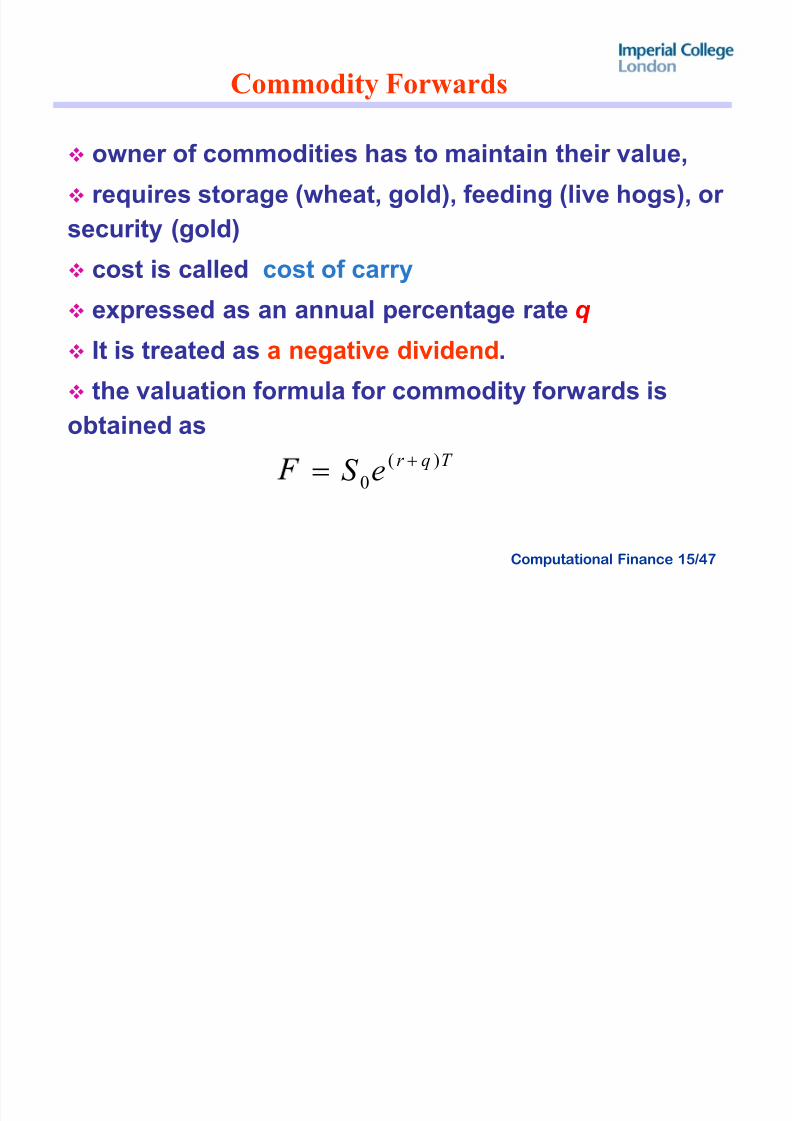
Commodity Forwards
owner of commodities has to maintain their value,
requires storage (wheat, gold), feeding (live hogs), or
security (gold)
cost is called cost of carry expressed as an annual percentage rate q
It is treated as a negative dividend.
the valuation formula for commodity forwards is
obtained asT qr eS )(
0
!
8/7/2019 Options Parity
http://slidepdf.com/reader/full/options-parity 16/47
Computational Finance 16/47
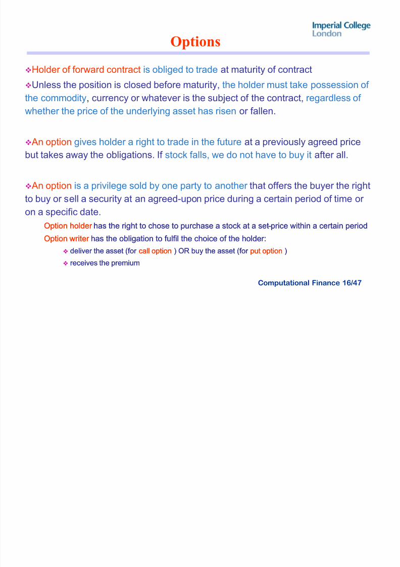
Options
Holder of forward contract is obliged to trade at maturity of contractUnless the position is closed before maturity, the holder must take possession of
the commodity, currency or whatever is the subject of the contract, regardless of
whether the price of the underlying asset has risen or fallen.
An option gives holder a right to trade in the future at a previously agreed pricebut takes away the obligations. If stock falls, we do not have to buy it after all.
An option is a privilege sold by one party to another that offers the buyer the right
to buy or sell a security at an agreed-upon price during a certain period of time or
on a specific date.Option holder Option holder has the right to chose to purchase a stock at a sethas the right to chose to purchase a stock at a set--price within a certain periodprice within a certain period
Option writer Option writer has the obligation to fulfil the choice of the holder:has the obligation to fulfil the choice of the holder:
deliver the asset (for deliver the asset (for call optioncall option ) OR buy the asset (for ) OR buy the asset (for put optionput option ))
receives the premiumreceives the premium
8/7/2019 Options Parity
http://slidepdf.com/reader/full/options-parity 17/47
Computational Finance 17/47
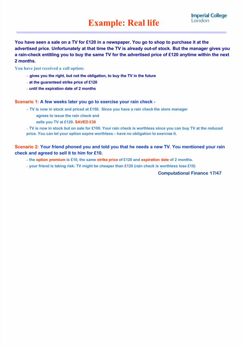
Example: R eal life
You have seen a sale on a TV for £120 in a newspaper. You go to shop to purchase it at theadvertised price. Unfortunately at that time the TV is already out-of stock. But the manager gives you
a rain-check entitling you to buy the same TV for the advertised price of £120 anytime within the next
2 months.
You have just received a call option:
± gives you the right, but not the obligation, to buy the TV in the future
± at the guaranteed strike price of £120
± until the expiration date of 2 months
Scenario 1: A few weeks later you go to exercise your rain check -
± TV is now in stock and priced at £150. Since you have a rain check the store manager
agrees to issue the rain check and
sells you TV at £120. SAVED £30
± TV is now in stock but on sale for £100. Your rain check is worthless since you can buy TV at the reducedprice. You can let your option expire worthless ± have no obligation to exercise it.
Scenario 2: Your friend phoned you and told you that he needs a new TV. You mentioned your rain
check and agreed to sell it to him for £10.
± ± the option premium is £10, the same strike price of £120 and expiration date of 2 months.
± your friend is taking risk: TV might be cheaper than £120 (rain check is worthless lose £10)
8/7/2019 Options Parity
http://slidepdf.com/reader/full/options-parity 18/47
8/7/2019 Options Parity
http://slidepdf.com/reader/full/options-parity 19/47
8/7/2019 Options Parity
http://slidepdf.com/reader/full/options-parity 20/47
Computational Finance 20/47
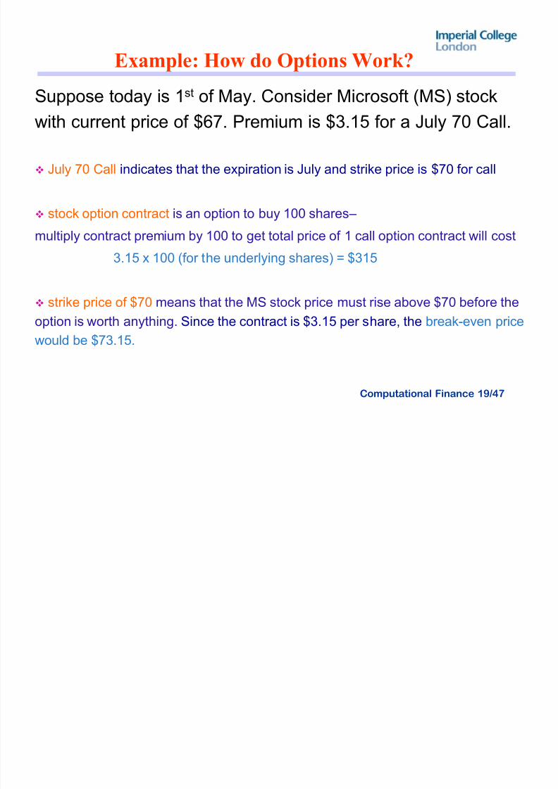
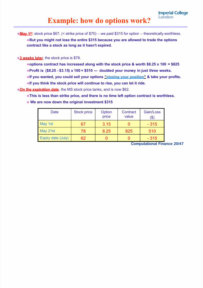
Example: how do options work?
May 1st: stock price $67, (< strike price of $70) ± we paid $315 for option ± theoretically worthless.
But you might not lose the entire $315 because you are allowed to trade the options
contract like a stock as long as it hasn't expired.
3 weeks later , the stock price is $78.
options contract has increased along with the stock price & worth $8.25 x 100 = $825
Profit is ($8.25 - $3.15) x 100 = $510 --- doubled your money in just three weeks.If you wanted, you could sell your options ³closing your position´ & take your profits.
If you think the stock price will continue to rise, you can let it ride.
On the expiration date, the MS stock price tanks, and is now $62.
This is less than strike price, and there is no time left option contract is worthless.
We are now down the original investment $315
Date Stock price Optionprice
Contractvalue
Gain/Loss
($)
May 1st 67 3.15 0 - 315
May 21st 78 8.25 825 510
Expiry date (July) 62 0 0 - 315
8/7/2019 Options Parity
http://slidepdf.com/reader/full/options-parity 21/47
Computational Finance 21/47
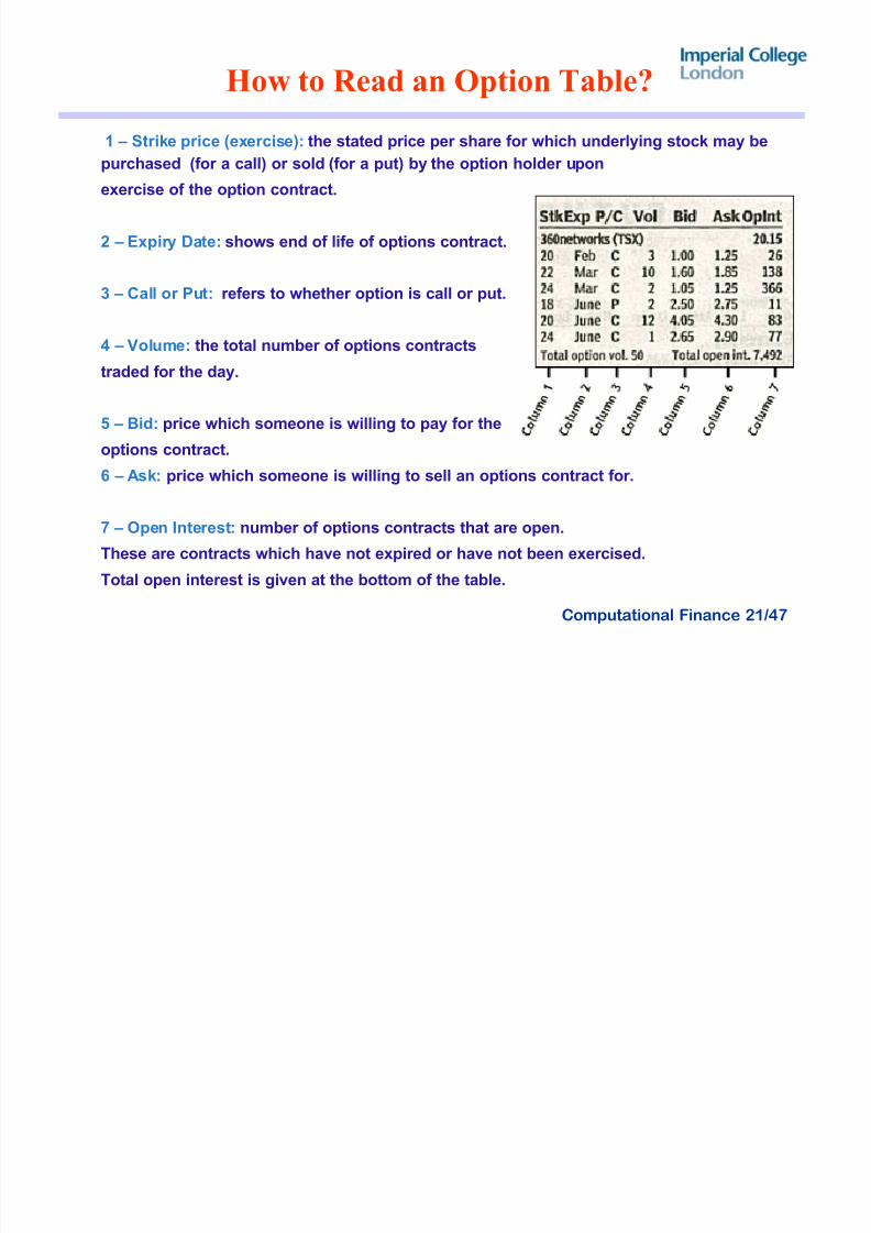
How to R ead an Option Table?
1 ± Strike price (exercise): the stated price per share for which underlying stock may be
purchased (for a call) or sold (for a put) by the option holder upon
exercise of the option contract.
2 ± Expiry Date: shows end of life of options contract.
3 ± Call or Put: refers to whether option is call or put.
4 ± Volume: the total number of options contracts
traded for the day.
5 ± Bid: price which someone is willing to pay for the
options contract.
6 ± Ask: price which someone is willing to sell an options contract for.
7 ± Open Interest: number of options contracts that are open.
These are contracts which have not expired or have not been exercised.
Total open interest is given at the bottom of the table.
8/7/2019 Options Parity
http://slidepdf.com/reader/full/options-parity 22/47
Computational Finance 22/47
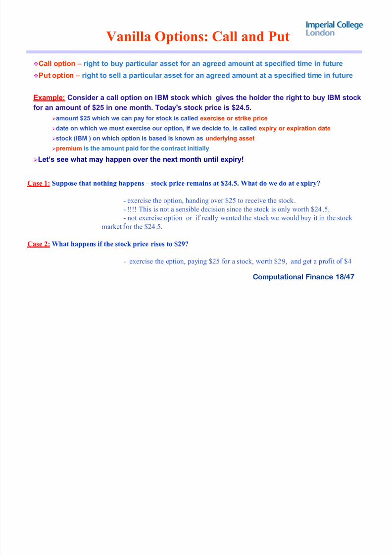
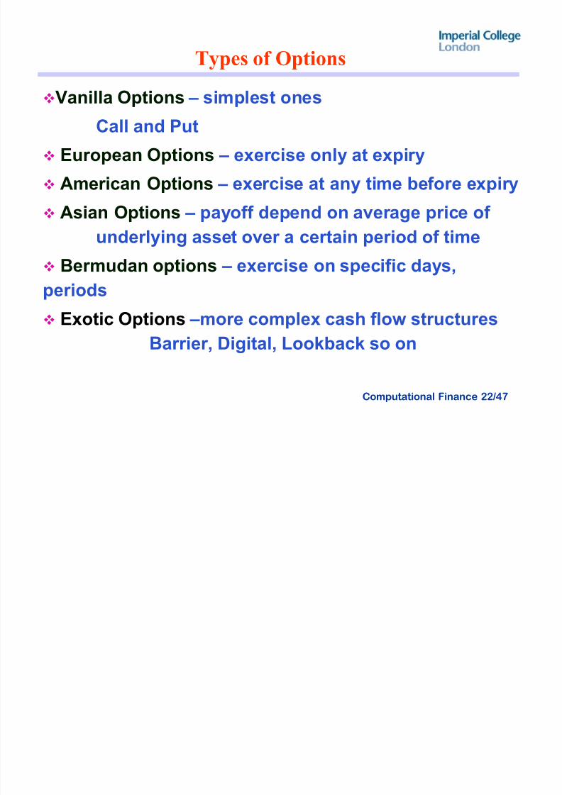
Types of Options
Vanilla Options ± simplest onesCall and Put
European Options ± exercise only at expiry
American Options ± exercise at any time before expiry
Asian Options ± payoff depend on average price of
underlying asset over a certain period of time
Bermudan options ± exercise on specific days,
periods Exotic Options ±more complex cash flow structures
Barrier, Digital, Lookback so on
8/7/2019 Options Parity
http://slidepdf.com/reader/full/options-parity 23/47
8/7/2019 Options Parity
http://slidepdf.com/reader/full/options-parity 24/47
Computational Finance 24/47
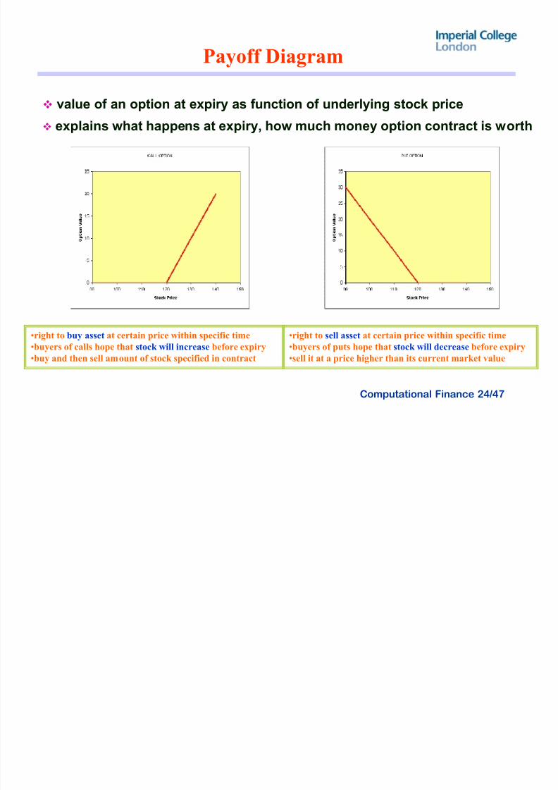
Payoff Diagram
value of an option at expiry as function of underlying stock price
explains what happens at expiry, how much money option contract is worth
�right to buy asset at certain price within specific time
�buyers of calls hope that stock will increase before expiry
�buy and then sell amount of stock specified in contract
�right to sell asset at certain price within specific time
�buyers of puts hope that stock will decrease before expiry
�sell it at a price higher than its current market value
8/7/2019 Options Parity
http://slidepdf.com/reader/full/options-parity 25/47
Computational Finance 25/47
Call Option Value at Expiry
Consider a call option with stock price and the exercise priceat the expiry date T
Value of a call option is zero or the difference between the value of
the underlying and strike price, whichever is greater.
If holder can purchase a share more cheaply in market
than by exercising option
If holder receives one share from writer of the call option
for price of
then make a profit of then make a profit of
T S E
0,max E S C T !
E S T
E S T
" E
E S T
8/7/2019 Options Parity
http://slidepdf.com/reader/full/options-parity 26/47
Computational Finance 26/47
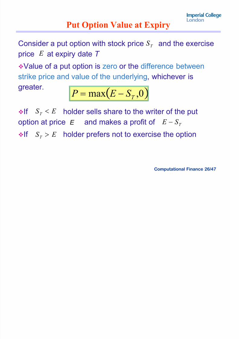
Put Option Value at Expiry
Consider a put option with stock price and the exerciseprice at expiry date T
Value of a put option is zero or the difference between
strike price and value of the underlying, whichever is
greater.
If holder sells share to the writer of the put
option at price E and makes a profit of
If holder prefers not to exercise the option
T S E
0,max T S E P !
E S T
E S T
T
S E
8/7/2019 Options Parity
http://slidepdf.com/reader/full/options-parity 27/47
Computational Finance 27/47
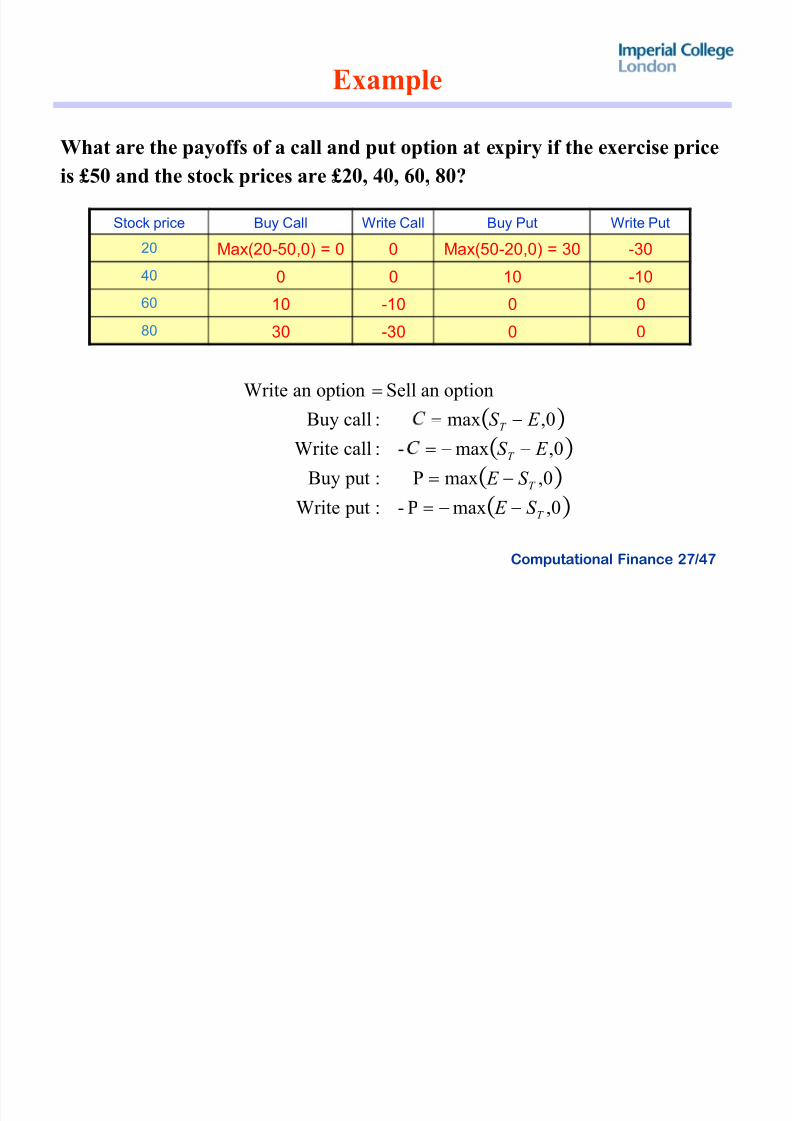
Example
Stock price Buy Call Write Call Buy Put Write Put
20 Max(20-50,0) = 0 0 Max(50-20,0) = 30 -30
40 0 0 10 -1060 10 -10 0 0
80 30 -30 0 0
What are the payoffs of a call and put option at expiry if the exercise price
is £50 and the stock prices are £20, 40, 60, 80?
0,maxP- : putWrite
0,maxP : putBuy
0,max- :callWrite0,max :callBuy
optionanSelloptionanWrite
T
T
T
T
S E
S E
E S
E S
!
!
!!
!
8/7/2019 Options Parity
http://slidepdf.com/reader/full/options-parity 28/47
Computational Finance 28/47
Example
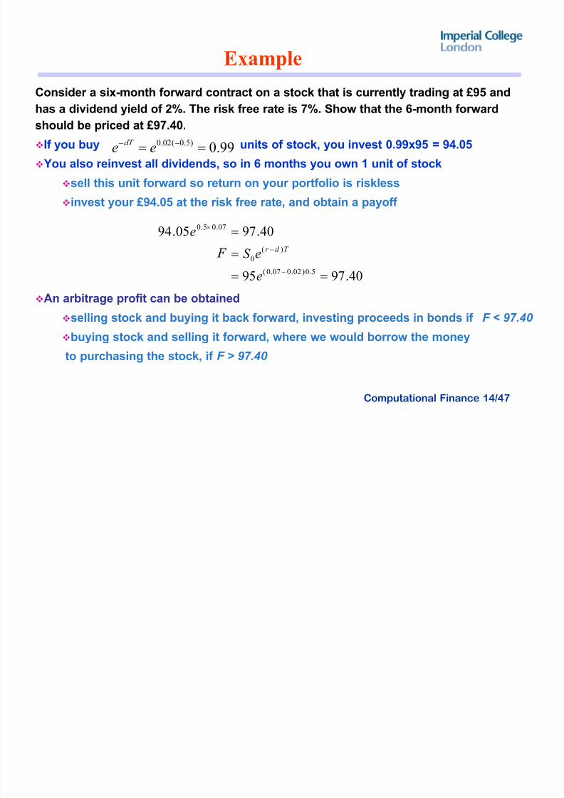
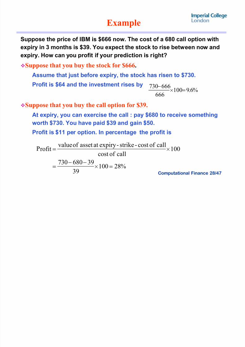
Suppose the price of IBM is $666 now. The cost of a 680 call option with
expiry in 3 months is $39. You expect the stock to rise between now and
expiry. How can you profit if your prediction is right?
Suppose that you buy the stock for $666.
Assume that just before expiry, the stock has risen to $730.
Profit is $64 and the investment rises by
Suppose that you buy the call option for $39.
At expiry, you can exercise the call : pay $680 to receive something
worth $730. You have paid $39 and gain $50.
Profit is $11 per option. In percentage the profit is
%6.9100666
666730 !v
%28100
39
39680730
100callof cost
callof cost-strike-expiryatassetof valuerofit
!v
!
v!
8/7/2019 Options Parity
http://slidepdf.com/reader/full/options-parity 29/47
Computational Finance 29/47
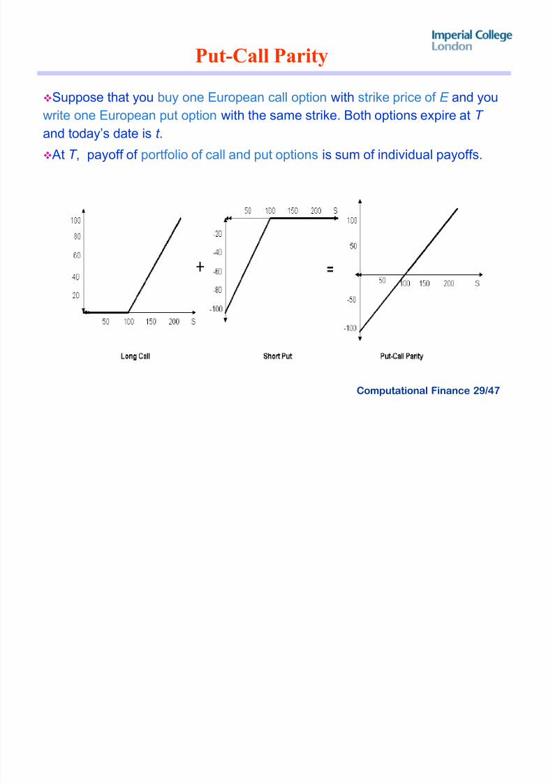
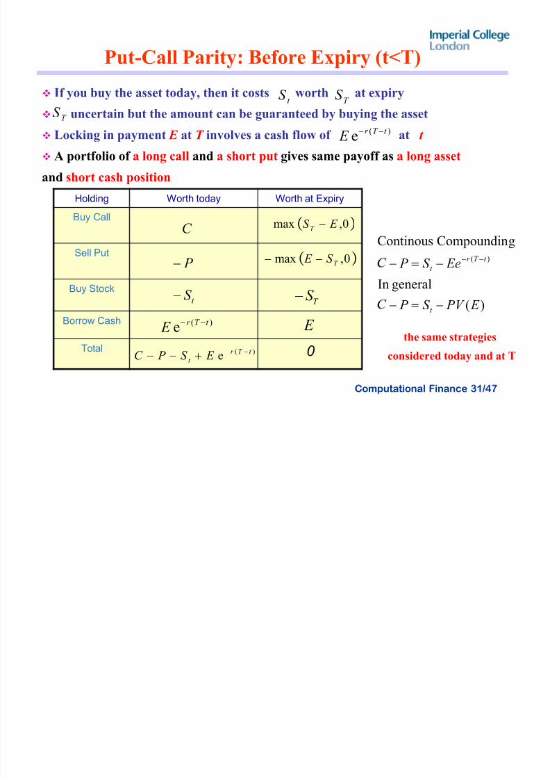
Put-Call Parity
Suppose that you buy one European call option with strike price of E and youwrite one European put option with the same strike. Both options expire at T
and today¶s date is t .
At T , payoff of portfolio of call and put options is sum of individual payoffs.
8/7/2019 Options Parity
http://slidepdf.com/reader/full/options-parity 30/47
Computational Finance 30/47
Put-Call Parity at T
Type Option Value
Call
Option
0
Put
Option
0
Portfolio
Value
C - P
0,max E S T !
E S T
0,max T S E P !
E S T
)( T S E
E S T
E S T E S T
E S P C
E S S E E S
T
T T T
!
! 0,max0,max
payoff of portfolio of call & put options
8/7/2019 Options Parity
http://slidepdf.com/reader/full/options-parity 31/47
8/7/2019 Options Parity
http://slidepdf.com/reader/full/options-parity 32/47
Computational Finance 32/47
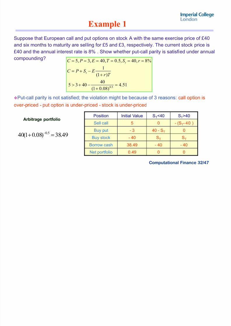
Example 1
Suppose that European call and put options on stock A with the same exercise price of £40
and six months to maturity are selling for £5 and £3, respectively. The current stock price is
£40 and the annual interest rate is 8% . Show whether put-call parity is satisfied under annual
compounding?
Put-call parity is not satisfied; the violation might be because of 3 reasons: call option is
over-priced - put option is under-priced - stock is under-priced
Arbitrage portfolio
51.4)08.01(
404035
)1(
1
%8,40,5.0,40,3,5
5.0!
"
!
!!!!!!
T r E S P C
r S T E P C
t
t
Position Initial Value ST<40 ST>40
Sell call 5 0 - (ST- 40 )
Buy put - 3 40 - ST 0
Buy stock - 40 ST ST
Borrow cash 38.49 - 40 - 40
Net portfolio 0.49 0 0
49.38)08.01(40 5.0 !
8/7/2019 Options Parity
http://slidepdf.com/reader/full/options-parity 33/47
Computational Finance 33/47
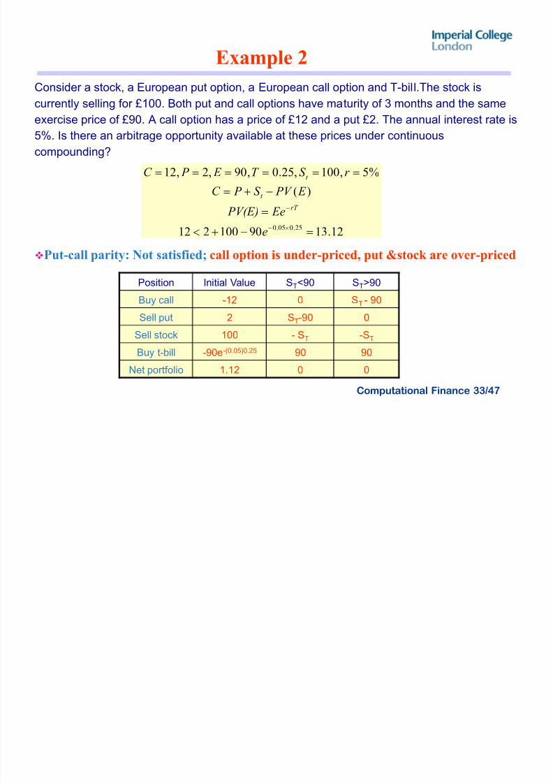
Example 2
Consider a stock, a European put option, a European call option and T-bill.The stock is
currently selling for £100. Both put and call options have maturity of 3 months and the sameexercise price of £90. A call option has a price of £12 and a put £2. The annual interest rate is
5%. Is there an arbitrage opportunity available at these prices under continuous
compounding?
Put-call parity: Not satisfied; call option is under-priced, put &stock are over-priced
12.1390100212
)(
%5,100,25.0,90,2,12
25.005.0 !
!
!
!!!!!!
v
e
E e PV ( E )
E PV S
P C
r S T E P C
rT
t
t
Position Initial Value ST<90 ST>90
Buy call -12 0 ST - 90
Sell put 2 ST-90 0
Sell stock 100 - ST -ST
Buy t-bill -90e-(0.05)0.25 90 90
Net portfolio 1.12 0 0
8/7/2019 Options Parity
http://slidepdf.com/reader/full/options-parity 34/47
Computational Finance 34/47
Option Pricing Models
Approaches to option pricing problem based on different
assumptions about market, dynamics of stock price behaviour
Theories based on the arbitrage principle,
applied when dynamics of underlying stock take certain forms
The simplest of these theories is based on binomial model of
stock price fluctuations
widely used in practice since it is simple and easy to calculate
approximation to movement of real prices
generalizes one period ³up-down´ model to multi-period setting
8/7/2019 Options Parity
http://slidepdf.com/reader/full/options-parity 35/47
Computational Finance 35/47
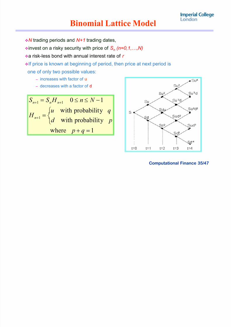
Binomial Lattice Model
N trading periods and N+1
trading dates,invest on a risky security with price of S n (n=0,1,«,N)
a risk-less bond with annual interest rate of r
If price is known at beginning of period, then price at next period is
one of only two possible values:
± increases with factor of u
± decreases with a factor of d
1 here y probabilitith
y probabilitith
10
1
11
!°
¯®
!
ee!
q p pd
qu H
N n H S S
n
nnn
8/7/2019 Options Parity
http://slidepdf.com/reader/full/options-parity 36/47
Computational Finance 36/47
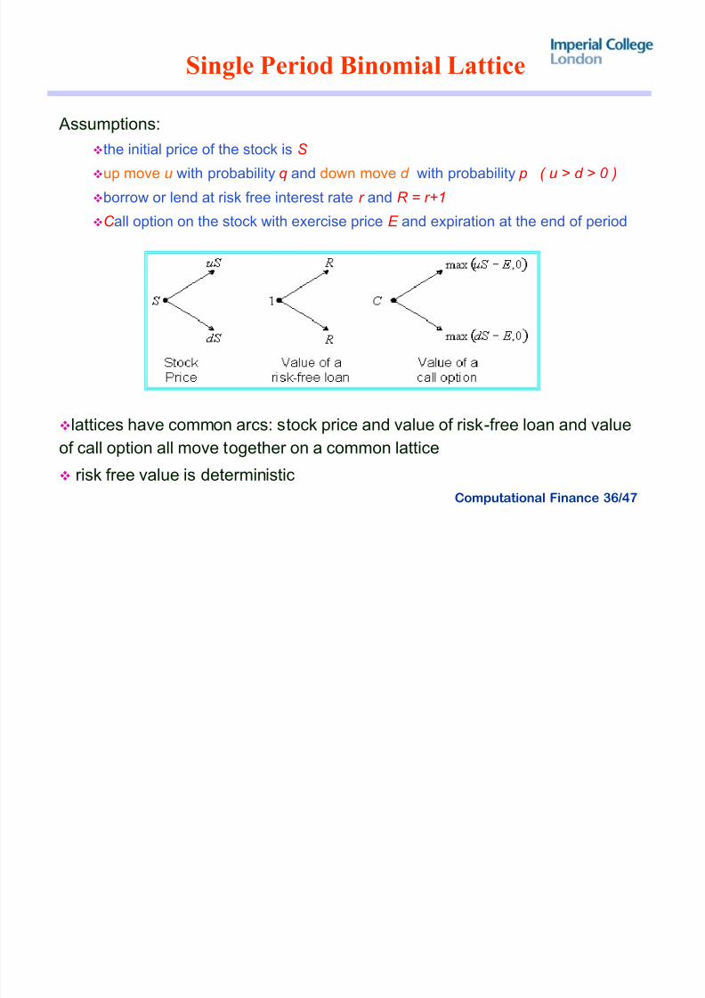
Single Period Binomial Lattice
Assumptions:the initial price of the stock is S
up move u with probability q and down move d with probability p ( u > d > 0 )
borrow or lend at risk free interest rate r and R = r +1
C all option on the stock with exercise price E and expiration at the end of period
lattices have common arcs: stock price and value of risk-free loan and value
of call option all move together on a common lattice
risk free value is deterministic
8/7/2019 Options Parity
http://slidepdf.com/reader/full/options-parity 37/47
Computational Finance 37/47
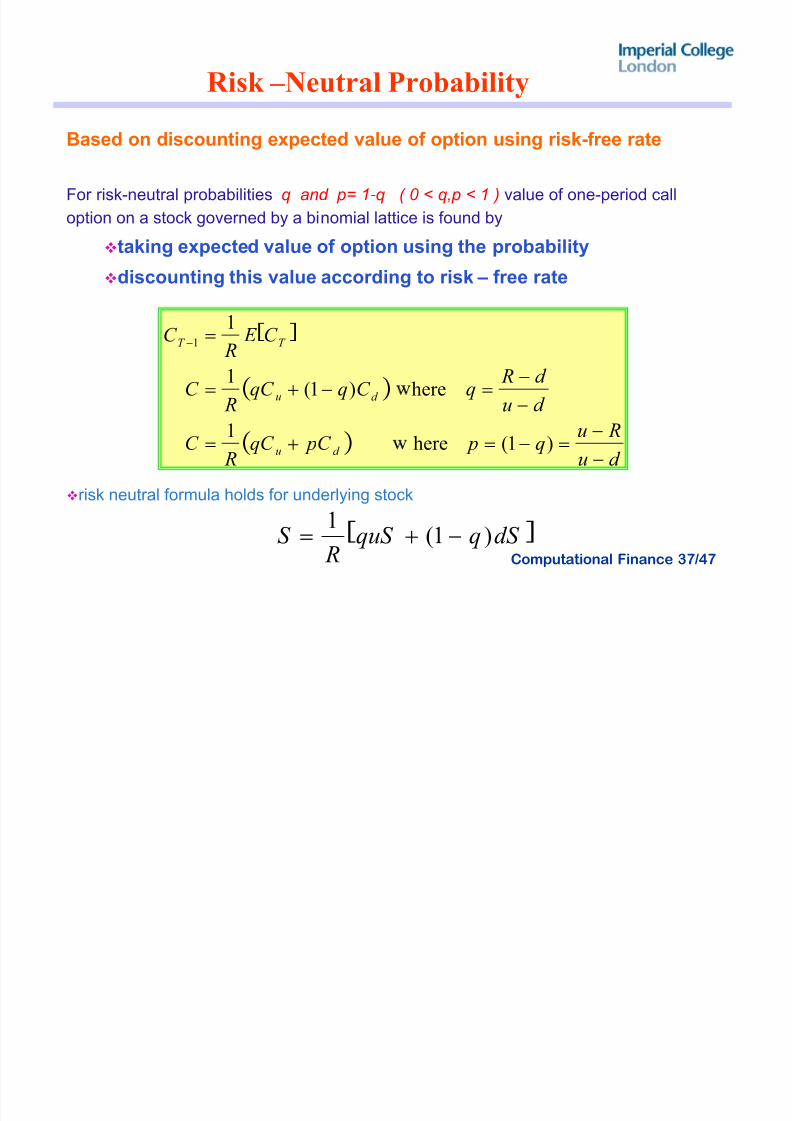
R isk ±Neutral Probability
Based on discounting expected value of option using risk-free rate
For risk-neutral probabilities q and p= 1-q ( 0 < q, p < 1 ) value of one-period call
option on a stock governed by a binomial lattice is found by
taking expected value of option using the probability
discounting this value according to risk ± free rate
risk neutral formula holds for underlying stock
? A
d u
Ruq p pC qC
RC
d u
d RqC qqC
RC
C E R
C
d u
d u
T T
!!!
!!
!
)1( here 1
here)1(1
11
? Ad S qquS
R
S )1(1
!
8/7/2019 Options Parity
http://slidepdf.com/reader/full/options-parity 38/47
8/7/2019 Options Parity
http://slidepdf.com/reader/full/options-parity 39/47
Computational Finance 39/47
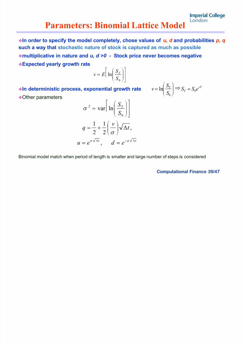
Parameters: Binomial Lattice Model
In order to specify the model completely, chose values of u , d and probabilities p, q
such a way that stochastic nature of stock is captured as much as possible
multiplicative in nature and u , d >0 - Stock price never becomes negative
Expected yearly growth rate
In deterministic process, exponential growth rate
Other parameters
Binomial model match when period of length is smaller and large number of steps is considered
¼½
»¬«
¹¹ º
¸©©ª
¨!
0
lnS
S E v T
vT T
T eS S S S v 0
0
ln !¹¹ º ¸©©
ª¨!
t t
T
ed eu
t
v
q
S
S
(( !!
(¹ º
¸
©ª
¨
!
¼½
»¬«
¹¹ º
¸©©ª
¨!
W W
W
W
,
,2
1
2
1
lnvar 0
2
8/7/2019 Options Parity
http://slidepdf.com/reader/full/options-parity 40/47
Computational Finance 40/47
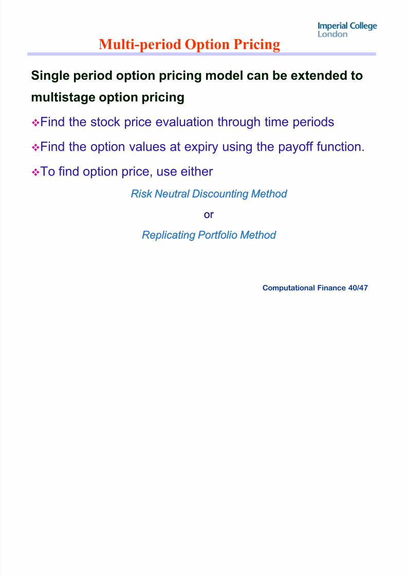
Multi-periodOption Pricing
Single period option pricing model can be extended to
multistage option pricing
Find the stock price evaluation through time periods
Find the option values at expiry using the payoff function.
To find option price, use either
Ri sk Neut ral Di scount ing M ethod Ri sk Neut ral Di scount ing M ethod
or or
R e pli c at ing P or tf oli o M ethod R e pli c at ing P or tf oli o M ethod
8/7/2019 Options Parity
http://slidepdf.com/reader/full/options-parity 41/47
Computational Finance 41/47
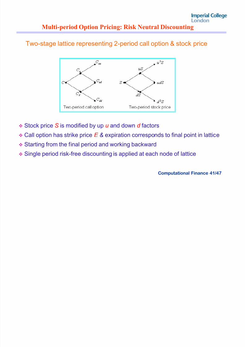
Multi-periodOption Pricing: R isk Neutral Discounting
Two-stage lattice representing 2-period call option & stock price
Stock price S is modified by up u and down d factors
Call option has strike price E & expiration corresponds to final point in lattice
Starting from the final period and working backward
Single period risk-free discounting is applied at each node of lattice
8/7/2019 Options Parity
http://slidepdf.com/reader/full/options-parity 42/47
Computational Finance 42/47
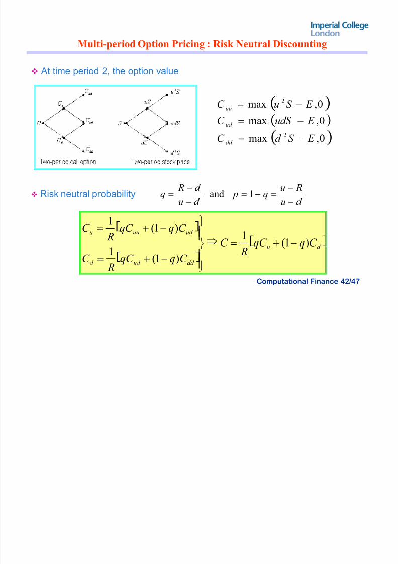
Multi-periodOption Pricing : R isk Neutral Discounting
At time period 2, the option value
Risk neutral probability
0,max
0,max
0,max
2
2
E S d C
E udS C
E S uC
dd
ud
uu
!
!
!
? A
? A
? Ad u
dd ud d
ud uuu
C qqC R
C
C qqC R
C
C qqC R
C
)1(1
)1(1
)1(1
!
±±À
±±¿
¾
!
!
d u
Ruq p
d u
d Rq
!!
! 1 and
8/7/2019 Options Parity
http://slidepdf.com/reader/full/options-parity 43/47
Computational Finance 43/47
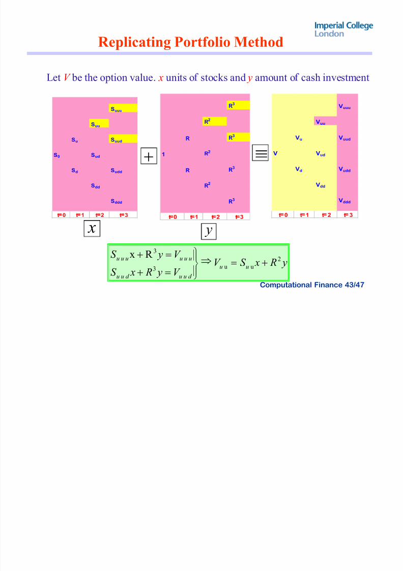
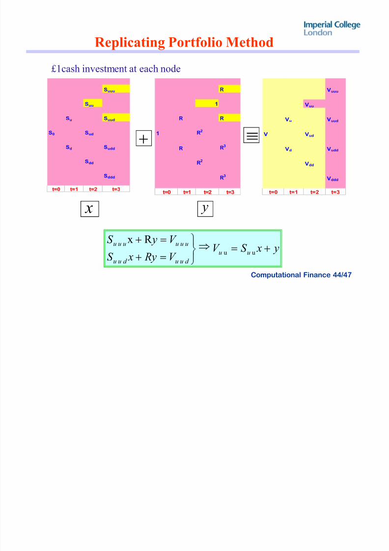
R eplicating Portfolio Method
Suuu
Suu
Su Suud
S0 Sud
Sd Sudd
Sdd
Sddd
t 0 t 1 t 2 t 3
R3
R2
R R3
1 R2
R R3
R2
R3
t 0 t 1 t 2 t 3
Vuuu
Vuu
Vu Vuud
V Vud
Vd Vudd
Vdd
Vddd
t 0 t 1 t 2 t 3
|
x y
y R xS V
V y R xS
V yS uu
d uud uu
uuuuuu 2
uu
3
3
R x!
±À
±¿¾
!
!
Let V be the option value. x units o stocks and y amount o cash investment
8/7/2019 Options Parity
http://slidepdf.com/reader/full/options-parity 44/47
Computational Finance 44/47
R eplicating Portfolio Method
Suuu
Suu
Su Suud
S0 Sud
Sd Sudd
Sdd
Sddd
t=0 t=1 t=2 t=3
R
1
R R
1 R2
R R3
R2
R3
t=0 t=1 t=2 t=3
Vuuu
Vuu
Vu Vuud
V Vud
Vd Vudd
Vdd
Vddd
t=0 t=1 t=2 t=3
|
x y
y xS V V R y xS
V yS uu
d uud uu
uuuuuu!
À¿¾
!
!uu
R x
£1cash investment at each node
8/7/2019 Options Parity
http://slidepdf.com/reader/full/options-parity 45/47
Computational Finance 45/47
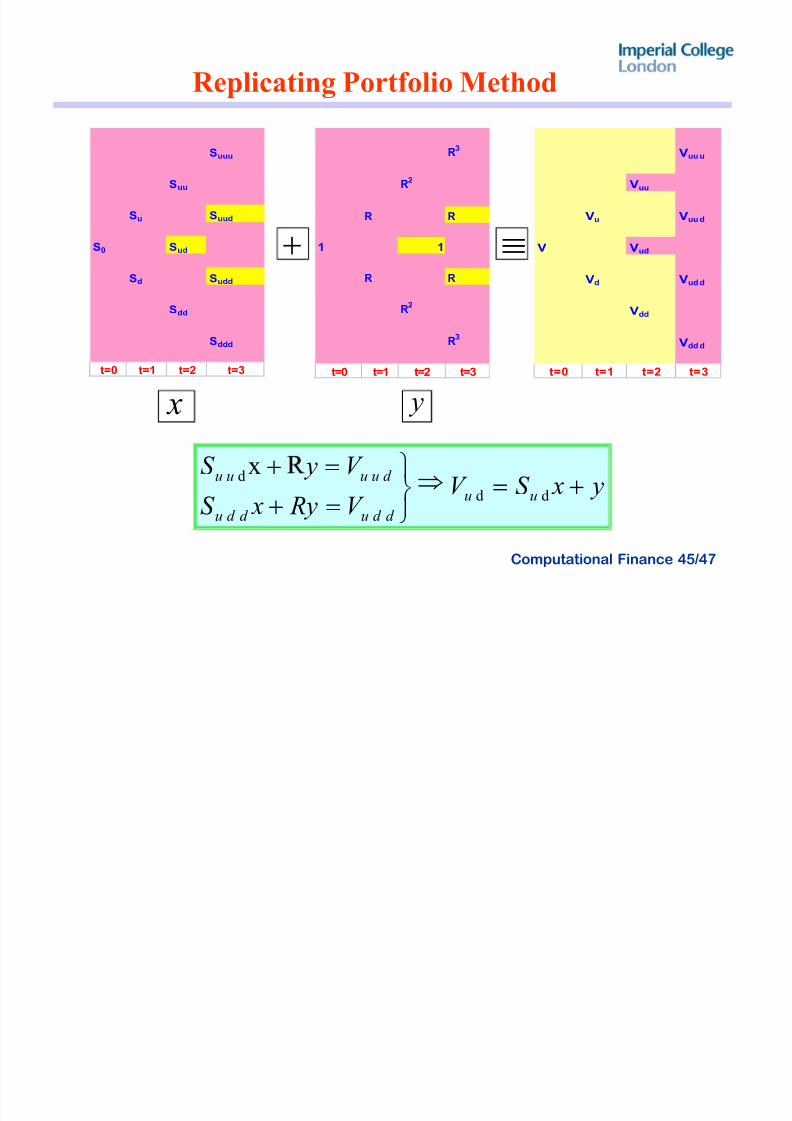
R eplicating Portfolio Method
|
x y
Suuu
Suu
Su Suud
S0 Sud
Sd
Sudd
Sdd
Sddd
t=0 t=1 t=2 t=3
R3
R2
R R
1 1
R R
R2
R3
t=0 t=1 t=2 t=3
Vuu u
Vuu
Vu Vuu d
V Vud
Vd
Vud d
Vdd
Vdd d
t=0 t=1 t=2 t= 3
y xS V V R y xS
V yS uu
d d ud d u
d uuuu!
À¿¾
!
!dd
d x
8/7/2019 Options Parity
http://slidepdf.com/reader/full/options-parity 46/47
Computational Finance 46/47
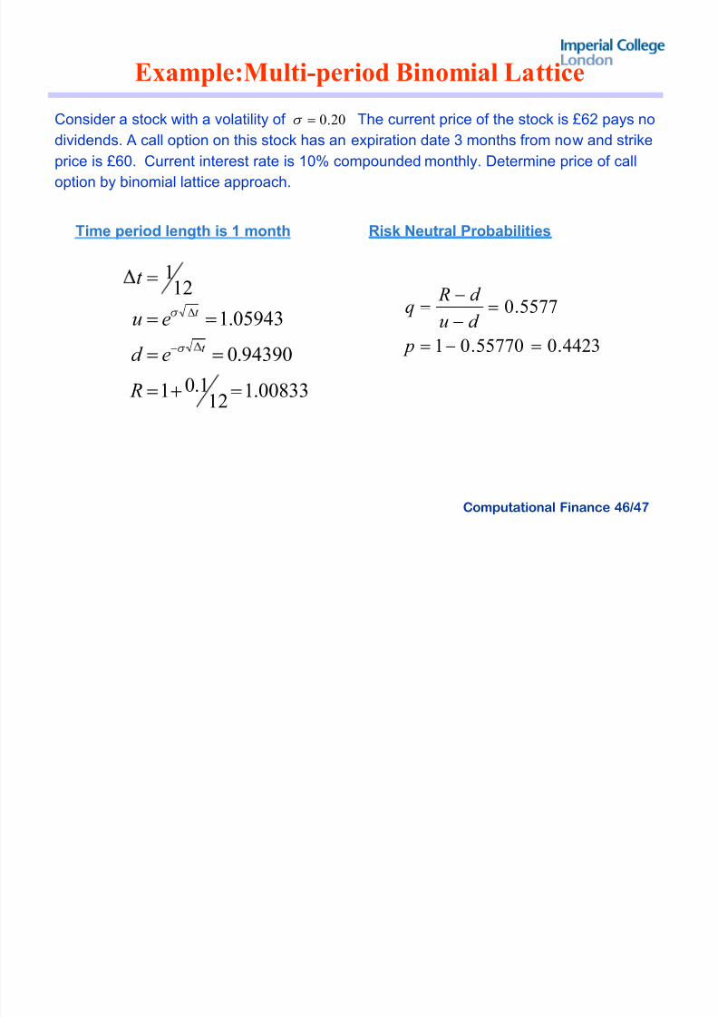
Example:Multi-period Binomial Lattice
Consider a stock with a volatility of The current price of the stock is £62 pays no
dividends. A call option on this stock has an expiration date 3 months from now and strike
price is £60. Current interest rate is 10% compounded monthly. Determine price of call
option by binomial lattice approach.
Time period length is 1 month Risk Neutral Probabilities
20.0!W
00833.112
1.01
94390.0
05943.1
121
!!
!!
!!
!
¡
(
R
ed
eu
t
t
t
W
W
4423.055770.01
5577.0
!!
!
!
p
d u
d Rq
8/7/2019 Options Parity
http://slidepdf.com/reader/full/options-parity 47/47
Computational Finance 47/47
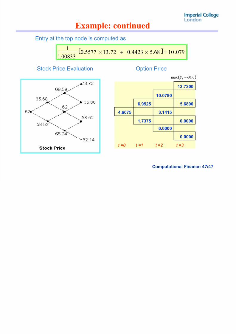
Example: continued
Entry at the top node is computed as
Stock Price Evaluation Option Price
13.7200
10.0790
6.9525 5.6800
4.6075 3.1415
1.7375 0.0000
0.0000
0.0000
t =0 t =1 t =2 t =3
? A 0791068544230721355770008331
1.....
.
!vv
0,60max T S