Option Pricing using L©vy Processes

CHALMERS∣∣∣ GOTEBORG UNIVERSITY

MASTER’S THESIS

Option Pricing using Levy Processes

YONGQIANG BU

Department of Mathematical Statistics

CHALMERS UNIVERSITY OF TECHNOLOGY

GOTEBORG UNIVERSITY

Goteborg, Sweden 2007

Thesis for the Degree of Master of Science (20 credits)

Option Pricing using Levy Processes

Yongqiang Bu

CHALMERS∣∣∣ GOTEBORG UNIVERSITY

Department of Mathematical Statistics

Chalmers University of Technology and Goteborg University

SE− 412 96 Goteborg, Sweden

Goteborg, June 2007

Abstract

In this Master’s thesis we price exotic options using Monte Carlo simulations. The assetprice process is modeled as an exponential Levy process. First we use Levy processes to fitthe log-returns of S&P 500 historical data. By means of both graphical and quantitative testswe find that the NIG process and the Meixner perform better than the Brownian motion.Secondly, we calibrate NIG, Meixner and CGMY Levy process models using S&P 500 indexvanilla options. The calibration results show that non-Gaussian Levy processes describes themarket price better than Brownian motion. At last, we use the calibrated models to priceexotic options.

Keywords: Barrier Option; Calibration; Exotic Option; Fast Fourier Transformation; LevyProcess; Monte-Carlo Simulation.

i

Acknowledgements

I would like to thank my supervisor Prof. Patrik Albin for his guidance and supportthroughout process of this thesis, as well as his encouragement and help during the past twoyears. I would also like to thank all members of staff at Chalmers, especially Ivar Gustafsson,Holger Rootzen, Hans Westergren, Nanny Wermuth, Nils Svanstedt, Peter Kumlin, MichaelPatriksson, Torgny Lindvall, Torbjorn Lundh, Serik Sagitov, Catalin Starica, Christer Borell,Erik Brodin, Viktor Olsbo and Mattias Sunden for their support to my study. I must thank toall my friends met at Gothenburg during the past two years. Finally, particularly to expressmy gratitude to my parents and my girlfriend, for their continued support and encouragement.

iii

Contents

1 Introduction 1

2 The Levy process framework 32.1 Levy processes . . . . . . . . . . . . . . . . . . . . . . . . . . . . . . . . . . . 32.2 Examples of Levy processes . . . . . . . . . . . . . . . . . . . . . . . . . . . . 3

2.2.1 Brownian motion . . . . . . . . . . . . . . . . . . . . . . . . . . . . . . 32.2.2 Normal inverse Gaussian process (NIG) . . . . . . . . . . . . . . . . . 42.2.3 Meixner process . . . . . . . . . . . . . . . . . . . . . . . . . . . . . . 42.2.4 CGMY process . . . . . . . . . . . . . . . . . . . . . . . . . . . . . . . 5

2.3 Modelling S&P 500 index with Levy processes . . . . . . . . . . . . . . . . . . 52.3.1 Stylized facts of financial time series . . . . . . . . . . . . . . . . . . . 62.3.2 Parameter estimation . . . . . . . . . . . . . . . . . . . . . . . . . . . 72.3.3 Test of distributional assumptions . . . . . . . . . . . . . . . . . . . . 8

3 Inverse model calibration 113.1 Risk-neutral option pricing . . . . . . . . . . . . . . . . . . . . . . . . . . . . 11

3.1.1 Equivalent martingale measure . . . . . . . . . . . . . . . . . . . . . . 123.2 Pricing formulas for European vanilla options . . . . . . . . . . . . . . . . . . 12

3.2.1 Black-Scholes formula . . . . . . . . . . . . . . . . . . . . . . . . . . . 123.2.2 Option pricing using fast Fourier transformation . . . . . . . . . . . . 13

3.3 Model calibration . . . . . . . . . . . . . . . . . . . . . . . . . . . . . . . . . . 153.4 Calibration results . . . . . . . . . . . . . . . . . . . . . . . . . . . . . . . . . 16

3.4.1 Data selection . . . . . . . . . . . . . . . . . . . . . . . . . . . . . . . . 163.4.2 Calibration results . . . . . . . . . . . . . . . . . . . . . . . . . . . . . 17

4 Exotic option pricing 214.1 Exotic options . . . . . . . . . . . . . . . . . . . . . . . . . . . . . . . . . . . 21

4.1.1 Barrier option . . . . . . . . . . . . . . . . . . . . . . . . . . . . . . . . 214.1.2 Lookback option . . . . . . . . . . . . . . . . . . . . . . . . . . . . . . 22

4.2 Pricing methods . . . . . . . . . . . . . . . . . . . . . . . . . . . . . . . . . . 224.2.1 Black-Scholes formula . . . . . . . . . . . . . . . . . . . . . . . . . . . 224.2.2 Monte Carlo pricing using Levy processes . . . . . . . . . . . . . . . . 234.2.3 Simulation techniques . . . . . . . . . . . . . . . . . . . . . . . . . . . 24

4.3 Results . . . . . . . . . . . . . . . . . . . . . . . . . . . . . . . . . . . . . . . . 25

5 Conclusion 29

v

A S&P 500 call option prices 33

vi

Chapter 1

Introduction

The beginning of modern mathematical finance can be attributed to Louis Bachelier who inyear 1900 proposed to model the price process {S(t)}t≥0 of an financial asset as

S(t) = S(0) + σ W (t),

where σ > 0 is a parameter and {W (t)}t≥0 is a standard Brownian motion.The main drawback of the Bachelier model is that it is possible for prices of financial assets

to becomes negative. Therefore Samuelson suggested the so called Bachelier-Samuelson model

S(t) = S(0) e(µ−σ2/2) t+σ W (t), (1.1)

where µ ∈ R is another parameter. In this model it is instead the log-price process log(S(t))that is a (not necessarily standard) Brownian motion (with drift).

In their seminal paper [3] Black and Scholes give a theoretically consistent frameworkfor option pricing based on the model (1.1). This paper changed the world of mathematicalfinance and initiated an strong growth of derivative markets. The Bachelier-Samuelson modelis therefore also called the Black-Scholes model (BS), depending on the context.

The Black-Scholes model assumes log-increments of the stock price are Gaussian. However,there is much empirical evidence for that these log-increments are not Gaussian. This hasled researchers to consider a variety of asset price models with non-Gaussian log-incrementsduring the last decade. One of the most important and natural family of such model is thatof exponential Levy processes. In turns out that such processes fit many empirically observedproperties of real world data much better than the Black-Scholes model.

In an exponential Levy process model the price process is given by

S(t) = S(0) eX(t) for t ≥ 0,

where {X(t)}t≥0 is a Levy process. Some of the most common Levy processes X that feature insuch exponential Levy process models are normal inverse Gaussian processes (NIG), Meixnerprocesses and CGMY processes. Note that the Black-Scholes model is also an exponentialLevy process model as Brownian motion with drift is a Levy process.

In this report we first show that NIG and Meixner Levy process models perform betterthan the Brownian motion when fitted to log-return of stock prices (Chapter 2). Then wecalibrate NIG, Meixner and CGMY Levy process models by an inverse approach where we fittheir predicted theoretical option prices to observed real world S&P 500 index vanilla optionprices (Chapter 3). Finally we use the latter calibration results together with Monte Carlosimulations to price European exotic options (Chapter 4).

1

Chapter 2

The Levy process framework

In this chapter we give the definitions of the Levy processes we will use in our work. We alsofit the corresponding exponential Levy process models to S&P 500 historical data.

2.1 Levy processes

We use the following definition of a Levy process from the book by Cont and Tankov [8]:

Definition 2.1 A cadlag1 real valued stochastic process {X(t)}t≥0 such that X(0) = 0 iscalled a Levy process if it has stationary independent increments and is stochastically con-tinuous.

An important feature of Levy process is their intimate link to infinite divisible distributions(e.g., Sato [13]): If {X(t)}t≥0}t≥0 is a Levy process, then every process value X(t) is infinitelydivisible. Conversely, to each infinitely divisible distribution there exist a unique in law Levyprocess {X(t)}t≥0 such that X(1) has that distribution.

Recall that a probability distribution on the real line is said to be infinitely divisible if forany integer n ≥ 1 there exists independent identically distributed random variables Y1, . . . , Yn

such that Y1 + ... + Yn has that distribution.From the above it follows that a Levy process {X(t)}t≥0}t≥0 has a unique so called char-

acteristic exponent in form of a continuous function ψ : R → R such that the characteristicfunction of X(t) is given by

E{eiuX(t)} = etψ(u) for u ∈ R and t > 0.

2.2 Examples of Levy processes

2.2.1 Brownian motion

Brownian motion with drift is a Levy process {X(t)}t≥0}t≥0 that has Gaussian increments.Specifically, X(t) is N(µt, σ2t)-distributed where σ > 0 and µ ∈ R are parameters.

1Right continuous with left limits.

3

2.2.2 Normal inverse Gaussian process (NIG)

The normal inverse Gaussian process (NIG) is a Levy process {X(t)}t≥0 that has normalinverse Gaussian distributed increments. Specifically, X(t) has a NIG(α, β, δt, µt)-distributionwith parameters α > 0, |β| < α, δ > 0 and µ ∈ R.

The NIG(α, β, δ, µ)-distribution has probability density function

fNIG(x;α, β, δ, µ) =αδ

π

K1

(α√

δ2 − (x− µ)2)

√δ2 + (x− µ)2

exp{δ√

α2 − β2 + β(x− µ)},

whereKv(z) =

12

∫ ∞

0uv−1 exp

{−z

2(u +

1u

)}

du

is the modified Bessel function of the third kind, while the characteristic function is given by

φNIG(u;α, β, δ, µ) = exp(−δ

(√α2 − (β + iu)2 −

√α2 − β2

))eiµu.

A NIG(α, β, δ, µ)-distributed random variable has the following stylized features:

Meanβδ√

α2 − β2+ µ

Varianceα2δ

(α2 − β2)3/2

Skewness3β

α√

δ(α2 − β2)1/4

Kurtosis 3(

1 +α2 + 4β2

δα2√

δ(α2 − β2)

)

See Barndorff-Nielsen [2] on more information about NIG processes.

2.2.3 Meixner process

The Meixner process is a Levy process {X(t)}t≥0 that has Meixner distributed increments.Specifically, X(t) has a Meixner(x; a, b, dt,mt)-distribution with parameters a > 0, |b| < π,d > 0 and m ∈ R.

The Meixner(x; a, b, dt,mt)-distribution has probability density function

fMeixner(x; a, b, d, m) =(2 cos(b/2))2d

2aπΓ(2d)exp

{b(x−m)a

} ∣∣∣Γ(d +

i(x−m))a

)∣∣∣2,

where Γ denotes the Gamma function, while the characteristic function is given by

φMeixner(u; a, b, d, m) =(

cos(b/2)cosh(au− ib)/2

)2d

eimu.

A Meixner(x; a, b, dt,mt)-distributed random variable has the following stylized features:

4

Mean ad tan(b/2) + m

Variance12

a2d

cos2(b/2)

Skewness sin(b/2)

√2d

Kurtosis 3 +2− cos(b)

d

See Schoutens [14] on more information about Meixner processes.

2.2.4 CGMY process

The CGMY process is a Levy process {X(t)}t≥0 such that X(1) is CGMY(C, G, M, Y )-distributed with parameters C, G, M > 0 and Y < 2.

The probability density function of a CGMY(C, G, M, Y )-distribution takes an analyti-cally very complicated form, while the characteristic function is given by

φCGMY(u;C, G, M, Y ) = exp{CΓ(−Y )((M − iu)Y −MY + (G + iu)Y −GY )

}.

A CGMY(C,G, M, Y )-distributed random variable has the following stylized features:

Mean C(MY−1 −GY−1)Γ(1− Y )

Variance C(MY−2 + GY−2)Γ(2− Y )

SkewnessC(MY−3 + GY−3)Γ(3− Y )

(C(MY−2 + GY−2)Γ(2− Y ))3/2

Kurtosis 3 +C(MY−4 + GY−4)Γ(4− Y )

(C(MY−2 + GY−2)Γ(2− Y ))2

See Carr, Geman, Madan and Yor [4] on more information about CGMY processes.

2.3 Modelling S&P 500 index with Levy processes

Our dataset will be the S&P 500 index adjust closed price from 3rd, June, 2002 to 3rd, June,2007, 1259 trading days, as listed by Yahoo Finance.

200 400 600 800 1000 1200

800

1000

1200

1400

Figure 2.1: S&P 500 index adjusted closed prices

5

200 400 600 800 1000 1200

-0.04

-0.02

0.02

0.04

Log returns

Figure 2.2: Log-return of S&P 500 index adjusted close prices

2.3.1 Stylized facts of financial time series

Now we discuss some stylized facts of financial time series, see Cont [6] for more information.

Skewness and kurtosis

Skewness and kurtosis of Gaussian distributions are 0 and 3, respectively. However, empiricalfinancial time series usually display non-zero skewness and higher kurtosis than 3. In our casethe skewness of the daily log-return of S&P 500 data is 0.191731 while the kurtosis is 6.68909.Hence it cannot be completely correct to model this data set with a Black-Scholes model.

Autocorrelations

Here we check the empirical autocorrelations (ACF) for log-return and squared log-returns ofour data set. For the definition of ACF, please check with any text book on time series:

0 50 100 150 200 250−0.2

0

0.2

0.4

0.6

0.8

Lag

Sam

ple

Aut

ocor

rela

tion

Sample Autocorrelation Function (ACF)

Figure 2.3: Empirical autocorrelations for log-returns

6

0 50 100 150 200 250−0.2

0

0.2

0.4

0.6

0.8

Lag

Sam

ple

Aut

ocor

rela

tion

Sample Autocorrelation Function (ACF)

Figure 2.4: Empirical autocorrelations for squared log-returns

From the above two figures we see that the log-returns are uncorrelated, while the squaredlog-returns instead are correlated. Hence it cannot even be completely correct to model thedata with an exponential Levy process model. However, we will not consider more generalmodels than that anyway.

Volatility clustering

Large changes in financial data tend to be followed by large changes, of either sign, while smallchanges tend to be followed by small changes, see Cont [7]. This experience is supported byFigure 2.4 above.

2.3.2 Parameter estimation

We will fit the empirical log-return of S&P 500 index to NIG process and Meixner process,as well as to Brownian motion by means of maximum likelihood estimation (MLE).

Due to the high numbers of parameters of the NIG and Meixner distribution and highnumbers of data points, it turned out to be close to impossibly time consuming to make adirect MLE fit with the help of standard mathematical software packages, see Jonsson [9].Therefore we used the methods of moments to get a first parameter estimate to be used asstarting point for the MLE fit in order to significantly speed up the fitting procedure. Theresults were as follows:

Brownian motion µ σ0.00031 0.0098

NIG a b d m78.3512 -5.70771 0.00756726 0.000862369

Meixner a b d m0.0279247 -0.178417 0.244316 0.000919888

7

The lack of an analytically tractable expression for the density function of CGMY distri-butions made us refrain from trying to fit CGMY processes.

2.3.3 Test of distributional assumptions

Here we consider two ways to evaluate the corectness of the fitted distributions.

Graphical test of distributional assumption

According to the Glivekno-Cantelli theorem, if the sample X1, ..., Xn has cummulative distri-bution function F (.; θ), then the ordered sample X(1) ≤ ... ≤ X(n) satisfies

limn→∞ max

1≤i≤n|(i− 0.5)/n− F (X(i); θ)| = 0,

so that a so called QQ-plot of

{(X(i), F−1((i− 0.5)/n); θ)}n

i=1

is an approximative 45o, and a systematic deviation therefrom indicates that the F (.; θ)assumption is not true.

The following three figures depict QQ-plots of our data set fitted to normal distribution,Meixner distribution and NIG distribution, respectively.

-0.02 -0.01 0.01 0.02

-0.03

-0.02

-0.01

0.01

0.02

0.03

Figure 2.5: Normal QQ-plot

-0.02 -0.01 0.01 0.02

-0.02

-0.01

0.01

0.02

Figure 2.6: Meixner QQ-plot

8

-0.02 -0.01 0.01 0.02

-0.02

-0.01

0.01

0.02

Figure 2.7: NIG QQ-plot

The QQ-plots indicate that the empirical data fits much better to the Meixner and NIGLevy process models than to the Brownian motion.

Statistical test of distributional assumptions

There are many analytical statistical tests for checking distributional assumptions. Amongthem the Kolmogorov-Smirnov distance (K-S) and Anderson & Darling statistic (A-D) [1] aretwo common choices.

Writing Femp for the empirical distribution of a data set and Ffit for the fitted distribution,the K-S distance is given by

KS = maxx∈R

|Femp(x)− Ffit(x)|,

while the A-D statistic is given by

AD = maxx∈R

|Femp(x)− Ffit(x)|√Ffit(x)(1− Ffit(x))

.

Note that the A-D statistic pays attention to the fit in the tails by mean of amplifying taildeviations as compared with the K-S statistic. This can be convenient, e.g., in applivationsto risk analysis etc.

We obtained the following values of the K-S and A-D statistics for our fitted distributions.

KS ADNormal 0.117641 0.272002

NIG 0.0321954 0.0963174Meixner 0.0190565 0.0487207

Table 2.1: K-S and A-D test statistics

The smaller value of K-S and A-D means closer of empirical distribution and fitted dis-tribution. Obviously, the statistic for Levy Process are smaller than the value for BrownianMotion. We find that the NIG process and the Meixner perform better than the Brownianmotion.

9

Chapter 3

Inverse model calibration

Before calibrating our Levy process models we have to introduce the risk-neutral optionpricing model.

3.1 Risk-neutral option pricing

We assume that the price B(t) of a risk-free asset satisfies the ordinary differential equation

dB(t) = r B(t) dt,

where r ≥ 0 is the interest rate. Further, we assume that there is a risky asset whose priceS(t) is given by

S(t) = S(0) eX(t),

where X(t) is a Levy process. In our case this Levy process will be of the type normal,Meixner, NIG or CGMY. The market does not admit arbitrage.

Recall that an arbitrage is a portfolio strategy such that one starts with zero capital andat some later time T is sure not to have lost money and has a positive probability to makemoney.

By the first fundamental theorem of asset pricing, if there exists a risk-neutral probabilitymeasure, then there is no arbitrage. This risk-neutral probability is a martingale measure Qthat is equivalent to the original probability measure P and such that the underlying assetprice is a Q local martingale.

See Shreve [17] on more information about the above matters.An European call option is the right but not obligation to buy a contingent claim at the

time of maturity T to a fix strike price K. Thus the payoff function is given by

max(S(T )−K, 0).

The arbitrage-free value of the option at time t < T can be defined as

Πt = e−r(T−t)EQ[max(S(T )−K, 0)], (3.1)

where Q is a risk-neutral measure.

11

3.1.1 Equivalent martingale measure

We must find an equivalent martingale measure in order to price the derivatives. For this wewill use the so called mean-correcting martingale measure.

After we have estimated all the parameters of some specific asset price process S(t), thenwe add a drift term ω ∈ R in a way appropriate to make the in this way discounted process amartingale. Specifically, writing q ∈ R for the dividend rate, in our exponential Levy processsetting, the condition

EQ[S(t)] = S(0) et(r−q)

gives thatω = r − q − log(φ(−i)),

where φ is the characteristic function of S(1).Here is a list of the mean-correcting risk neutral drift terms for the Levy processes we

consider:

Model ω

Normal r − q − µ

CGMY r − q − CΓ(−Y )((M − 1)Y −MY + (G + 1)Y −GY )NIG r − q + δ(

√(α2 − (β + 1)2 −

√(α2 − β2))

Meixner r − q − 2δ(log(cos β/2))− log(cos((α + β)/2))

3.2 Pricing formulas for European vanilla options

We consider the case of vanilla options for which the payoff function only depends on theterminal stock price. We can find an analytical price formula for Brownian motion basedprice models, but require numerical solutions for other Levy process based models.

3.2.1 Black-Scholes formula

With the volatility σ, the interest rate r and the dividend rate q in the exponential Brownianmotion Black-Scholes asset price model, the asset price S(t) at time t is given by

S(t) = S(0) exp{

σW (t) + (r − q − 12σ2)t

}.

AsS(T ) = S(t) exp

{σ(W (T )−W (t)) + (r − q − 1

2σ2)(T − t)

},

using (3.1), we get the option price

Πt = EQ[e−r(T−t)(S(T )−K)+

]

= EQ[e−r(T−t)(x eσ(W (T )−W (t))+(r−q− 1

2)(T−t)σ2 −K)+

]

= EQ[e−rτ (x e−σ

√τ Y )+(r−q− 1

2σ2)τ −K)+

],

where τ = T − t and

Y = −W (T )−W (t)√T − t

12

is a standard normal random variable. Writing

d1 = d2 + σ√

τ =1

σ√

τ

[log

( x

K

)+

(r − q +

12σ2

)τ],

we thus obtain

Πt =12π

∫ d2

−∞e−rτ

[x exp

{−σ√

τ y +(r − q − 1

2σ2

)τ}−K

]e−

12y2

dy

=12π

∫ d2

−∞x exp

{−σ√

τ y −(q +

12σ2

)τ − 1

2y2

}dy − 1

2π

∫ d2

−∞e−rτK e−

12y2

dy

=12π

∫ d2

−∞x e−qτ exp

{−1

2(y + σ

√τ)2

}dy − e−rτKΦ(d2)

= x e−qτΦ(d1)− e−rτKΦ(d2) (3.2)

If we insert S(t) instead of x in the (3.2), then we get the option pricing at time t.

3.2.2 Option pricing using fast Fourier transformation

For more general Levy process models than those based on Brownian motion we typicallycannot find analytical solutions in the fashion of (3.2). We will therefore now introducepricing methods based on characteristics function. When using these methods in practice fastFourier transformation can be employed, see Carr and Madan [5] on more information.

The Fourier transform of an option price

Here we will evaluate an European call option price based on the price asset price processS(t), maturity time T and strike price K. Write k = log(K) and s(T ) = log(S(T )). LetCT (k) denote the option price and qT the risk-neutral probability density function of the logprice sT .

The characteristic function of the density qT is given by

φT (u) =∫ ∞

−∞eiusqT (s) ds.

The option value which is related to the risk-neutral density qT is given by

CT (k) =∫ ∞

ke−rT

(es − ek

)qT (s) ds.

Here CT (k) is not square integrable because when k → −∞ so that K → 0, we have CT →S(0). To obtain a square integrable function, Carr and Madan [5] suggested consideration ofthe modified price cT (k) given by

cT (k) = eαkCT (k),

for a suitable α > 0. Here Carr and Madan suggested to choose α ≈ 0.25, while Schoutens[15] suggests α ≈ 0.75. The value of α affects the speed of convergence.

The Fourier transform of cT (k) is given by

ψT (υ) =∫ ∞

−∞eiυkcT (k) dk.

13

The inverse corresponding inverse Fourier transform takes the form

cT (k) =12π

∫ ∞

−∞e−iυkψT (υ) dυ.

We can use these formulas to get the following option price formula for CT (k):

CT (k) =exp(−αk)

2π

∫ ∞

−∞e−iυkψT (υ) dυ =

exp(−αk)π

∫ ∞

0e−iυkψT (υ) dυ, (3.3)

where we made use of the fact that the function ψT is odd in its imaginary part and even inits real part since CT (k) is real.

We may express ψT in terms of φT (k) as

ψT (υ) =∫ ∞

−∞eiυk

∫ ∞

keαke−rT (es − ek)qT (s) dsdk

=∫ ∞

−∞e−rT qT (s)

∫ s

−∞(es+αk − ek+αk)eiυkdkds

=∫ ∞

−∞e−rT qT (s)

(e(α+1+iυ)s

α + iυ− e(α+1+iυ)s

α + 1 + iυ

)ds

= e−rT

∫ ∞

−∞qT (s)

e(α+1+iυ)s

(α + iυ)(α + 1 + iυ)ds

=e−rT φT (υ − (α + 1)i)

α2 + α− υ2 + i(2α + 1)υ. (3.4)

Using known expressions for the characteristic function of NIG, CGMY and Meixner in(3.4), we can use (3.3) to get the option price.

Fast Fourier transformation

Fast Fourier transformation (FFT) is an efficient algorithm to compute the following sum

ω(k) =N∑

j=1

e−i2π(j−1)(k−1)/Nx(j), (3.5)

where N is usually a power of 2. FFT is a commonly employed discrete approximationtechnique of Fourier transform used to reduce computational labour.

Here we will reexpress the relation (3.3) approximately using the FFT (3.5) as

CT (k) ≈ exp(−αk)π

N∑

j=1

e−iυjkψT (υj)η (3.6)

with the following conventions and parameter values (as suggested by Carr and Madan [5])

υj = η(j − 1), N = 4096, a = Nη = 600, b =Nλ

2, ku = −b +

2b

N(u− 1), λη =

2π

N.

Here a is the upper limit for the integration, while ku is a vector with N values of k and bsets a bound on the log strike to range between −b and b.

14

Our formula (3.6) for CT can now be rewritten as

CT (k) ≈ exp(−αku)π

N∑

j=1

e−iλη(j−1)(u−1)eibυjψT (υj)η.

Here we cannot combine a too fine integration grid with a wide enough region for strikes, asif we choose a too small η we get a fine integration grid but few strikes lying in the region.

Carr and Madan suggest to use Simpson’s weighting rule to obtain an accurate integrationwith large η. Then we rewrite our price formula as

CT (k) ≈ exp(−αku)π

N∑

j=1

e−i2π(j−1)(u−1)/NeibυjψT (υj)η

3(3 + (−i)j − δj−1

), (3.7)

where δn is the Kronecker delta function.We will use Black-Scholes formula for the normal model together with (3.7) for our other

Levy process based models to compute call option prices.

3.3 Model calibration

In this section we use historical option prices to calibrate model parameters. In this way weavoid many problems that are associated with calibrations that are based on the underlyingasset prices.

While the pricing problem is concerned with computing option values given the modelparameters, the calibration problem is concerned with computing the model parameters giventhe option prices. Thus the calibration problem is the inverse problem to the pricing problem.

One of the most popular calibration methods are to use least squares, they idea of which isvery simple: Observed market prices (Ci)N

i=1 at t = 0 with different strikes (Ki) and maturities(Ti) should be the same as those proposed by the risk-neutral model prices Cθ described inlast section with the model parameters θ. Thus we find the best parameter values θ by meansof minimizing the sum of quadratic deviations between these prices

θ∗ = arg minN∑

i=1

(Cθ(Ti,Ki)− Ci)2. (3.8)

We will compute the following statistics suggested by Schoutens [15] to measure the qualityof fits:

APE =N∑

i=1

|Cθ(Ti,Ki)− Ci)|N

/ N∑

i=1

Ci

N,

AAE =N∑

i=1

|Cθ(Ti,Ki)− Ci)|N

,

ARPE =1N

N∑

i=1

|Cθ(Ti,Ki)− Ci)|Ci

,

RMSE =

√√√√N∑

i=1

(Cθ(Ti,Ki)− Ci))2

N.

15

3.4 Calibration results

We use S&P 500 historical call option prices on 1st of June 2007 from Yahoo Finance thatare listed in Appendix A below. The market prices were chosen from June 2007 to December2008. The strike is from 1300 to 2000 with the increment of 25 from 1300 to 1700 and theincrement 100 from 1700 to 2000. The index closed price is 1536.34.

Some of the options have two different prices with the same maturity and strike. In thatcase, we choose the price with highest trading volume. We didn’t include the option pricesthat were smaller than 1.

3.4.1 Data selection

There are four different versions of the option prices, namely the close price, the bid, the askand the mean of the bid and ask.

1300 1400 1500 1600 1700 1800 1900 20000

50

100

150

200

250

300

350

Strike

Pric

e

Close PriceBid PriceAsk PriceMean of Bid and Ask Price

Figure 3.1: Option data set

Although very few paper discuss the selection of data set, it is crucial for the calibrationresults. In particular, for some option with low volume, there are big difference between theclose prices and bid ask prices. This can be explained by that for frequently traded optionsthe bid and ask prices match, while for some little traded options the last trade date mightbe long time ago, so that the last trade does not express the true value of option.

From the above figure we see that the close prices have a lot of outliers compare to bidand ask. Thus we conclude that the bid and ask prices are better to use than the close prices.The following table show the results of the calibrations of NIG using the bid, the ask as wellas the mean of bid and ask:

16

NIG Bid Ask Mean of bid and askAPE 0.0176 0.0137 0.0140AAE 2.2634 1.7956 1.8120ARPE 0.1089 0.0840 0.0894RMSE 0.9162 0.3381 0.1501

Table 3.1: NIG Calibration Statistics

From the above table we conclude that calibration using mean of bid and ask is slightlybetter than bid and ask. All of these three in turn are much better than using close prices.Thus we will use the mean of bid and ask as our option market data to calibrate models.

3.4.2 Calibration results

the following tables show the calibrated model parameters together with the correspondingvalues of APE, AAE, ARPE and RMSE.

Models ParametersNormal σ

0.1531CGMY C G M Y

0.0156 0.0767 7.5500 1.2996NIG α β θMeixner 5.0364 -3.3199 0.0881

α β θ0.3400 -1.4900 0.2900

Table 3.2: Calibration results

Normal CGMY Meixner NIGAPE 0.0575 0.0121 0.0120 0.0140AAE 7.4543 1.5632 1.5553 1.8120ARPE 0.3093 0.0793 0.0846 0.0894RMSE 1.0244 0.0026 0.0426 0.1501

Table 3.3: APE, AAE, ARPE and RMSE for calibrations

The calibrations for CGMY, NIG and Meixner are quite similar in quality and all performmuch better than calibration for Normal. Hence we can get improvements if we employ moregeneral Levy processes that Brownian motion in option pricing.

We remark here that the model parameters we got from our calibrations are differentfrom those obtained by the more conventional calibration method to fit the exponential Levyprocess asset price model to real world asset prices underlying the option.

The following four figures show the theoretical option prices from our calibrations togetherwith the corresponding market option prices.

17

1300 1400 1500 1600 1700 1800 1900 20000

50

100

150

200

250

300

350

Strike

Pric

e

Market PriceModel Price

Figure 3.2: Normal calibration to S&P 500 option prices

1300 1400 1500 1600 1700 1800 1900 20000

50

100

150

200

250

300

350

Strike

Pric

e


Figure 3.3: NIG calibration to S&P 500 option prices

18

1300 1400 1500 1600 1700 1800 1900 20000

50

100

150

200

250

300

350

Strike

Pric

e


Figure 3.4: CGMY calibration to S&P 500 option prices

1300 1400 1500 1600 1700 1800 1900 20000

50

100

150

200

250

300

350

Strike

Pric

e


Figure 3.5: Meixner calibration to S&P 500 option prices

19

Chapter 4

Exotic option pricing

The option we have discussed until now is the vanilla option which means the payoff functiononly depend on terminal value. However, path-dependent options have become popular in theOTC market in the last twenty years. Barrier option and lookback option are two importantexamples of such so called exotic options.

In this chapter we will consider barrier options and discuss their pricing methods basedon our previous calibration results. Before discussing the pricing methods we describe thebarrier option in more detail.

4.1 Exotic options

4.1.1 Barrier option

The holder of a barrier option has the right to buy or sell an asset at a specific price at theend of the contract. The payoff function of a barrier option depends on whether the price ofthe underlying asset crossses a given threshold the barrier before maturity.

There are two types barrier option, namely knock-in options and knock-out options. Aknock-in options is activated only when the underlying asset touches the barrier, while aknock-out option is instead deactivated when it touches the barrier. For each type of barrieroption, there is an up option and down option version opf it. Thus we have four types ofbarrier call options: down-and-out barrier call, down-and-in barrier call, up-and-in barriercall and up-and-out barrier call.

Let us assume that the duration of the contract is T . Define the maximum and minimumasset price process up til time t ∈ [0, T ] as

M(t) = sup{S(u) : 0 ≤ u ≤ t} and m(t) = inf{S(u) : 0 ≤ u ≤ t},

respectively. See Schoutens [15, 16] on more details.

Up-and-in barrier call

The up-and-in barrier call option is a standard European call option with strike K when itsmaximum lies above the barrier H, while it is worthless otherwise. The initial price is giveby

CUI = e−rTEQ[(S(T )−K)+1M(T )≥H

].

21

Up-and-out barrier call

The up-and-out barrier call option is a standard European call option with strike K when itsmaximum lies below the barrier H, while it is worthless otherwise. The initial price is giveby

CUO = e−rTEQ[(S(T )−K)+1M(T )<H

].

Down-and-in barrier call

The down-and-in barrier call option is a standard European call option with strike K whenits minimum lies below the barrier H, while it is worthless otherwise. The initial price is giveby

CDI = e−rTEQ[(S(T )−K)+1m(T )≤H

].

Down-and-out barrier call

The down-and-out barrier call option is a standard European call with strike K when its liesabove some barrier H, while it is worthless otherwise. The initial price is give by

CDO = e−rTEQ[(S(T )−K)+1m(T )>H

].

4.1.2 Lookback option

The paper by Nguyen-Ngo [11] treats exotic options for underlying exponential Levy processasset price models. For exotic option base on exponential Brownian motion, see Shreve [17].

There are two types of lookback options, namely fixed and floating strike lookback option.Here we only consider the fixed strike option.

The payoff function of fixed strike lookback option is the difference between the stockterminal value and its lowest value during the option lifetime. The price is given by

CL = e−rTEQ[S(T )−m(T )

].

4.2 Pricing methods

The main problem with barrier option pricing is to find the distribution of minimum and max-imum processes m and M . It is possible to obtain the explicit proce formluas in Black-Scholesnormal framework. However, the distribution of minima and maxima of more general Levyprocesses is usually not known explicitly. We will therefore use the Monte Carlo simulationtechniques to estimate the exotic option process. See Schoutens [15, 16] on more details.

4.2.1 Black-Scholes formula

The closed-form solution for the Brownian motion framework attributed to Merton, Reinerand Rubinstein gives the formulas for the types of exotic we consider as

CDO = S(0)Φ(x1) e−qT −K e−rT Φ(x1 − σ√

T − S(0) e−qT( H

S(0)

)2λΦ(y1)

+K e−rT( H

S(0)

)2λ−2Φ(y1 − σ

√T )

22

CUI = S(0)Φ(x1) e−qT −K e−rT Φ(x1 − σ√

T )− S(0) e−qT( H

S(0)

)2λ(Φ(−y)− Φ(−y1))

+K e−rT( H

S(0)

)2λ−2(Φ(−y + σ

√T )− Φ(y1 + σ

√T )

)

CDI = e−rTEQ[(S(T )−K)+

]− CDO

CUO = e−rTEQ[(S(T )−K)+

]− CUI

for H > K, while

CDI = S(0) e−qT( H

S(0)

)2λΦ(y)−K e−rT

( H

S(0)

)2λ−2Φ(y − σ

√T )

CUO = 0CDO = e−rTEQ

[(S(T )−K)+

]− CDI

CUI = e−rTEQ[(S(T )−K)+

]

for H ≤ K, where

λ =1σ2

(r − q +

σ2

2

),

y =1

σ√

Tlog

( H2

S(0)K

)+ λσ

√T ,

x1 =1

σ√

Tlog

(S(0)H

)+ λσ

√T ,

y1 =1

σ√

Tlog

( H

S(0)

)+ λσ

√T .

Moreover, for the lookback option in the Brownian motion framework, we have

CL = S(0) e−qT(Φ(a1)− σ2

2(r − q)Φ(−a1)

)− S(0) e−rT

(Φ(a2)− σ2

2(r − q)Φ(−a2)

),

where

a1 =1σ

(r − q +

σ2

2

)√T and a2 =

1σ

(r − q − σ2

2

)√T .

4.2.2 Monte Carlo pricing using Levy processes

It is not possible to get the closed-form exotic option prices for the more general Levy processthan Brownian motion we consider. Hence we will use Monte Carlo methods to find theseoption prices.

The Monte Carlo Pricing procedure goes as follows:

1. Calibrate the model on the vanilla option prices available in the market (S&P 500 calloption in our case) and find the risk-neutral parameters of the model. (This procedurehas already been carried out in a previous chapter.)

2. Simulate N trajectories of the calibrated Levy process based models.

3. Calculate the payoff function pi for each trajectory, i = 1, . . . , N .

4. Calculate the sample mean payoff to get the estimated payoff p =∑N

i=1 pi/N .

5. Discount the estimated payoff at the risk-free rate and get the derivative price erT p.

23

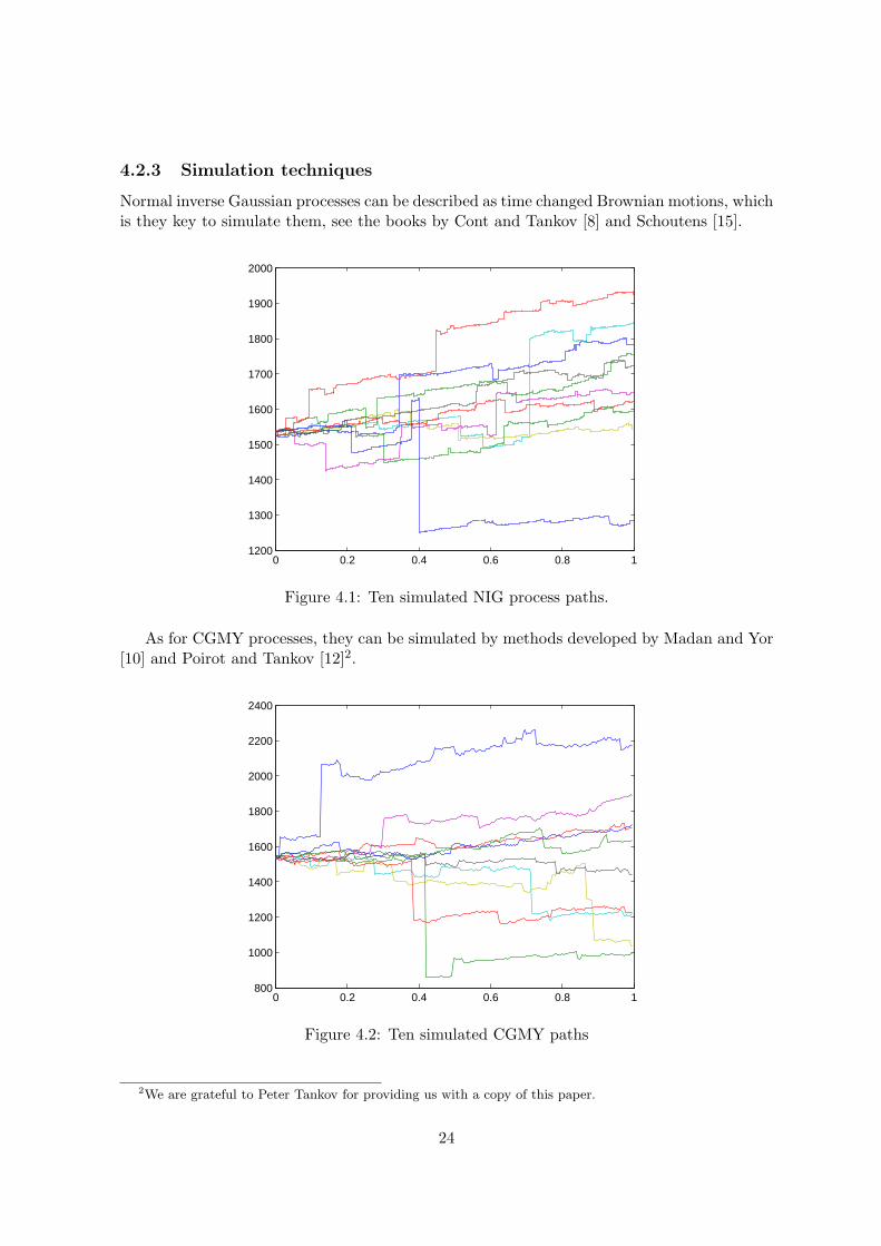
4.2.3 Simulation techniques

Normal inverse Gaussian processes can be described as time changed Brownian motions, whichis they key to simulate them, see the books by Cont and Tankov [8] and Schoutens [15].

0 0.2 0.4 0.6 0.8 11200

1300

1400

1500

1600

1700

1800

1900

2000

Figure 4.1: Ten simulated NIG process paths.

As for CGMY processes, they can be simulated by methods developed by Madan and Yor[10] and Poirot and Tankov [12]2.

0 0.2 0.4 0.6 0.8 1800

1000

1200

1400

1600

1800

2000

2200

2400

Figure 4.2: Ten simulated CGMY paths

2We are grateful to Peter Tankov for providing us with a copy of this paper.

24

We will not discuss simulation techniques for Meixner processes, and thus not considerexotic option pricing based on Meixner processes.

4.3 Results

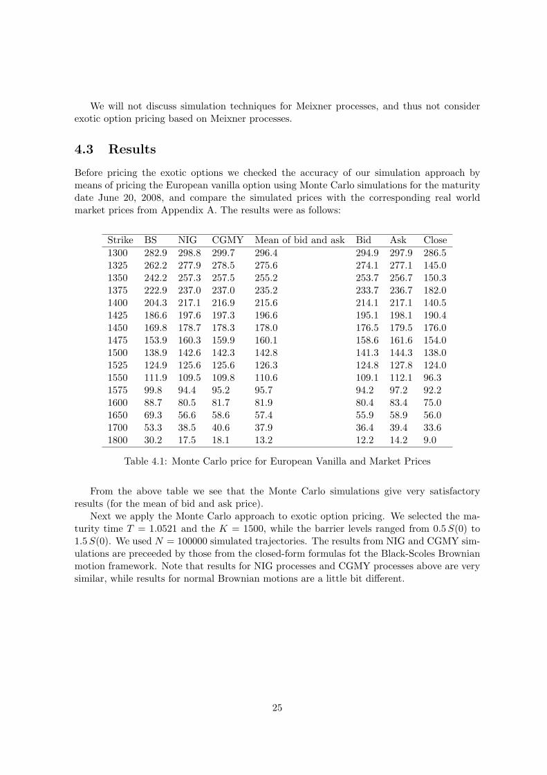
Before pricing the exotic options we checked the accuracy of our simulation approach bymeans of pricing the European vanilla option using Monte Carlo simulations for the maturitydate June 20, 2008, and compare the simulated prices with the corresponding real worldmarket prices from Appendix A. The results were as follows:

Strike BS NIG CGMY Mean of bid and ask Bid Ask Close1300 282.9 298.8 299.7 296.4 294.9 297.9 286.51325 262.2 277.9 278.5 275.6 274.1 277.1 145.01350 242.2 257.3 257.5 255.2 253.7 256.7 150.31375 222.9 237.0 237.0 235.2 233.7 236.7 182.01400 204.3 217.1 216.9 215.6 214.1 217.1 140.51425 186.6 197.6 197.3 196.6 195.1 198.1 190.41450 169.8 178.7 178.3 178.0 176.5 179.5 176.01475 153.9 160.3 159.9 160.1 158.6 161.6 154.01500 138.9 142.6 142.3 142.8 141.3 144.3 138.01525 124.9 125.6 125.6 126.3 124.8 127.8 124.01550 111.9 109.5 109.8 110.6 109.1 112.1 96.31575 99.8 94.4 95.2 95.7 94.2 97.2 92.21600 88.7 80.5 81.7 81.9 80.4 83.4 75.01650 69.3 56.6 58.6 57.4 55.9 58.9 56.01700 53.3 38.5 40.6 37.9 36.4 39.4 33.61800 30.2 17.5 18.1 13.2 12.2 14.2 9.0

Table 4.1: Monte Carlo price for European Vanilla and Market Prices

From the above table we see that the Monte Carlo simulations give very satisfactoryresults (for the mean of bid and ask price).

Next we apply the Monte Carlo approach to exotic option pricing. We selected the ma-turity time T = 1.0521 and the K = 1500, while the barrier levels ranged from 0.5 S(0) to1.5 S(0). We used N = 100000 simulated trajectories. The results from NIG and CGMY sim-ulations are preceeded by those from the closed-form formulas fot the Black-Scoles Brownianmotion framework. Note that results for NIG processes and CGMY processes above are verysimilar, while results for normal Brownian motions are a little bit different.

25

0.5 1 1.50

20

40

60

80

100

120

140

Barrier as Percentage of Spot

Opt

ion

Price

BS−CUOBS−CUI

Figure 4.3: Brownian motion barrier as percentage of spot

0.5 1 1.50

20

40

60

80

100

120

140


Opt

ion

Price

BS−CDOBS−CDI

Figure 4.4: Brownian motion barrier as percentage of spot

26

0.5 1 1.50

50

100

150


Opt

ion

Price

NIG−CUONIG−CUI

Figure 4.5: NIG barrier as percentage of spot

0.5 1 1.50

50

100

150


Opt

ion

Price

NIG−CDONIG−CDI

Figure 4.6: NIG barrier as percentage of spot

27

0.5 1 1.50

50

100

150


Opt

ion

Price

CGMY−CUOCGMY−CUI

Figure 4.7: CGMY barrier as percentage of spot

0.5 1 1.50

50

100

150


Opt

ion

Price

CGMY−CDOCGMY−CDI

Figure 4.8: CGMY barrier as percentage of spot

28

Chapter 5

Conclusion

In this master thesis, we focus on the Option Pricing using Levy processes. We started withdefinition of Levy process and the examples of Levy process.

We use Maximum-likelihood estimation to estimate the parameters and show that Levyprocess fit the log-returns of of S&P 500 historical data better than Brownian Motion bymeans of both graphical and quantitative tests. However, for the distribution which do nothave closed-form, this method cannot be used. Secondly, we price the option price using fastfourier transformation for Levy process since it is easy to find the characteristic function formost of the Levy process.The calibration results show that non-Gaussian Levy processes de-scribes the market price better than Brownian motion. At last, we use the calibration resultto price exotic option using Monte Carlo simulation.

We also test the selection of dataset. The results show that using mean of bid and ask isslightly better than bid and ask. All of these three in turn are much better than using closeprices.

In the future work, it would be interested to calibrate inverse problem with more optiondata. We also need to consider the Levy process with stochastic volatility.

29

Bibliography

[1] Anderson, T.W. and Darling, D.A. (1954). A test of goodness of fit. Journal of the Amer-ican Statistical Association 49 765-769.

[2] Barndorff-Nielsen,O.E. (1995). Normal inverse Gaussian distributions and the modell-ing of stock returns. Reasearch Report, Department of Theoretical Statistics, AarhusUniversity.

[3] Black, F. and Scholes, M. (1973). The pricing of options and corporate liabilities. Journalof Political Economy 81 637-654.

[4] Carr, P., Geman, H., Madan, D.H. and Yor, M. (2002). The fine structure of assetreturns: an empirical investigation. Journal of Business 75 305-332.

[5] Carr, P. and Madan, D.H. (1998). Option valuation using the fast Fourier transform.Journal of Computational Finance 2 61-73.

[6] Cont, R. (2001). Empirical properties of asset returns: stylized facts and statistical issues.Quantitative Finance 1 223-236.

[7] Cont, R. (2005). Volatility clustering in financial markets: Empirical facts and agent-based models. In: Long-Memory in Economics, G. Teyssire and A. Kirman Ed’s. Spring-er Verlag, Heidelberg.

[8] Cont, R. and Tankov, P. (2004). Financial Modelling with Jump Processes. Chapman &Hall, New York.

[9] Jonsson, F. (2004). On the fitting of generalized hyperbolical distributions to financialdata. Master’s thesis, Department of Mathematical Statistics, Chalmers University ofTechnology.

[10] Madan, D.B. and Yor, M. (2005). CGMY and Meixner subordinators are absolutelycontinuous with respect to one sided stable subordinators. Prepublication, Laboratoirede Probabilites et Modeles Aleatories.

[11] Nguyen-Ngoc, L. (2003). Exotic options in general exponential Levy models. Prepubli-cation, Universites Paris 6.

[12] Poirot, J. and Tankov, P. (2006). Monte Carlo option pricing for tempered stable(CGMY) processes. Unpublished manuscript.

[13] Sato, K. (1999). Levy Process and Infinitely Divisible Distributions. Cambridge Univer-sity Press, Cambridge.

31

[14] Schoutens, W. (2002). Meixner Process: Theory and application in Finance. EURAN-DOM Report, EURANDOM, Eindhoven.

[15] Schoutens, W. (2003). Levy Process in Finance: Pricing Financial Derivatives. Wiley,New York.

[16] Schoutens, W. (2006). Exotic options under Levy models: An overview. Journal of Com-puational and Applied Mathematics 189 526-538.

[17] Shreve, S.E. (2004). Stochastic Calculus for Finance II: Continous-Time Models. Spring-er Verlag, New York.

32

Appendix A

S&P 500 call option prices

We collected 100 call option prices for the S&P 500 index at the close of market on Jun,1,2007from Yahoo Finance. The closed index price is S0 = 1536.34. We selected the risk free interestrate 0.05 and dividend yield 0.019. The depicted prices are the mean of bid and ask pricesthat we used for our calibrations.

Strike Jun 15 Jul 20 Sep 21 Dec 21 Mar 21 Jun 20 Dec 192007 2007 2007 2007 2008 2008 2008

1300 239.1 244.5 254.0 268.5 296.4 322.91325 214.2 220.0 230.4 246.0 275.6 303.21350 189.3 195.6 207.1 223.9 239.6 255.2 283.91375 164.5 171.4 184.1 202.2 235.2 265.01400 139.7 147.4 161.5 181.0 198.5 215.6 246.51425 114.9 123.7 139.4 160.4 178.8 196.6 228.31450 90.4 100.5 118.1 140.4 159.6 178.0 210.71475 66.05 78.2 97.7 121.2 141.1 160.1 193.51500 42.85 56.9 78.4 103.0 123.4 142.8 176.81525 22.25 38.3 60.6 85.8 106.5 126.3 160.81550 6.95 22.25 44.4 69.9 90.7 110.6 145.31575 1.275 10.75 31.0 55.4 75.9 95.71600 1.15 4.5 20.1 42.6 62.4 81.9 116.31650 6.6 22.8 39.6 57.41700 10.3 22.9 37.9 67.81800 1.25 13.2 34.21900 14.42000 5.0

33

Option Pricing using L©vy Processes

Documents

Transcript of Option Pricing using L©vy Processes