
OPTION PRICING AND HEDGING A DISSERTATIONqx719jf6675/Thesis-augmented.… · dissertation...
108
OPTION PRICING AND HEDGING WITH TRANSACTION COSTS A DISSERTATION SUBMITTED TO THE DEPARTMENT OF STATISTICS AND THE COMMITTEE ON GRADUATE STUDIES OF STANFORD UNIVERSITY IN PARTIAL FULFILLMENT OF THE REQUIREMENTS FOR THE DEGREE OF DOCTOR OF PHILOSOPHY Ling Chen August 2010
Transcript of OPTION PRICING AND HEDGING A DISSERTATIONqx719jf6675/Thesis-augmented.… · dissertation...
OPTION PRICING AND HEDGING
WITH TRANSACTION COSTS
A DISSERTATION
SUBMITTED TO THE DEPARTMENT OF STATISTICS
AND THE COMMITTEE ON GRADUATE STUDIES
OF STANFORD UNIVERSITY
IN PARTIAL FULFILLMENT OF THE REQUIREMENTS
FOR THE DEGREE OF
DOCTOR OF PHILOSOPHY
Ling Chen
August 2010

http://creativecommons.org/licenses/by-nc/3.0/us/
This dissertation is online at: http://purl.stanford.edu/qx719jf6675
© 2010 by Ling Chen. All Rights Reserved.
Re-distributed by Stanford University under license with the author.
This work is licensed under a Creative Commons Attribution-Noncommercial 3.0 United States License.
ii

I certify that I have read this dissertation and that, in my opinion, it is fully adequatein scope and quality as a dissertation for the degree of Doctor of Philosophy.
Tse Lai, Primary Adviser
I certify that I have read this dissertation and that, in my opinion, it is fully adequatein scope and quality as a dissertation for the degree of Doctor of Philosophy.
Balakanapathy Rajaratnam
I certify that I have read this dissertation and that, in my opinion, it is fully adequatein scope and quality as a dissertation for the degree of Doctor of Philosophy.
Guenther Walther
Approved for the Stanford University Committee on Graduate Studies.
Patricia J. Gumport, Vice Provost Graduate Education
This signature page was generated electronically upon submission of this dissertation in electronic format. An original signed hard copy of the signature page is on file inUniversity Archives.
iii
Abstract
The traditional Black-Scholes theory on pricing and hedging of European call options
has long been criticized for its oversimplified and unrealistic model assumptions. This
dissertation investigates several existing modifications and extensions of the Black-
Scholes model and proposes new data-driven approaches to both option pricing and
hedging for real data.
The semiparametric pricing approach initially proposed by Lai and Wong (2004)
provides a first attempt to bridge the gap between model and market option prices.
However, its application to the S&P 500 futures options is not a success, when the
original additive regression splines are used for the nonparametric part of the pricing
formula. Having found a strong autocorrelation in the time-series of the Black-Scholes
pricing residuals, we propose a lag-1 correction for the Black-Scholes price, which es-
sentially is a time-series modeling of the nonparametric part in the semiparametric
approach. This simple but efficient time-series approach gives an outstanding pric-
ing performance for S&P 500 futures options, even compared with the commonly
practiced and favored implied volatility approaches.
A major type of approaches to option hedging with proportional transaction costs
is based on singular stochastic control problems that seek an optimal balance between
the cost and the risk of hedging an option. We propose a data-driven rule-based
strategy to connect the theoretical approaches with real-world applications. Similar to
the optimal strategies in theory, the rule-based strategy can be characterized by a pair
of buy/sell boundaries and a no-transaction region in between. A two-stage iterative
procedure is provided for tuning the boundaries to a long period of option data.
Comparing the rule-based strategy with several other existing hedging strategies,
iv

we obtain favorable results in both the simulation studies and the empirical study
using the S&P 500 futures and futures options. Making use of a reverting pattern
of the S&P 500 futures price, we refine the rule-based strategy by allowing hedging
suspension at large jumps in futures price.
v
Acknowledgements
I would like to take this opportunity to thank all the people who have helped me
during my five-year study and pursuit of the doctorate at Stanford.
First and foremost, I would like to express my deepest gratitude to my advisor,
Professor Tze Leung Lai, for his invaluable guidance and encouragement in my study,
my research and many other aspects of my life at Stanford. He is always approachable
and willing to spare me his time for discussions and chats. The high standards he sets
for the quality of my work have prompted me to grow into a more mature researcher.
I have also benefited from his enlightening advice on my career choice. It is honor
and a great experience to have worked with and mentored by him. I, among his
many students, have been influenced by his diligence, positive attitude and pleasant
personality.
I would like to thank Professor Kay Giesecke, Professor James Primbs, Professor
Bala Rajaratnam and Professor Guenther Walther for serving on my oral exam com-
mittee. Their insightful questions and constructive suggestions are all great resources
for the completion and enhancement of this dissertation. Special thanks go to Pro-
fessor Bala Rajaratnam and Professor Guenther Walther for the time and effort they
spent on reading this whole dissertation.
I am also grateful to Professor Tiong Wee Lim of National University of Singapore
for much of the foundation work that he has done with Professor Lai, providing
a promising starting point for my work. We had lots of fruitful discussions and
cooperation during his visits to Stanford. I am indebted to him for sharing with me
the S&P 500 futures option data and his computer codes for handling them.
The first three years of my study and research at Stanford was supported by
vi

Stanford Graduate Fellowship. Herein I would also like to thank the sponsor of my
fellowship for the great honor and financial support.
My peer students and friends at Stanford have lent enormous help and support to
me, both in academics and in life. Among them are Anwei Chai, Hao Chen, Su Chen,
Yi Fang Chen, Shaojie Deng, Victor Hu, Kshitij Khare, Luo Lu, Li Ma, Zongming
Ma, Paul Pong, Kevin Sun, Yunting Sun, Kevin Wu, Wei Wu, Ya Xu, Feng Zhang,
Kaiyuan Zhang and Baiyu Zhou. This is, however, far from a complete list of names.
Our friendship and the fun we had together will remain a treasure for my entire life.
Lastly but most importantly, I would like to thank my parents for everything that
they have been giving me. Any words I put down here cannot compare with their
enduring love and support for me. I would more like to share with them my happiness
and excitement at this moment, and I know for sure that they will be even happier
and more excited than I am. To my Mom, Mingyan Wu, and my Dad, Lunian Chen,
I dedicate this dissertation.
vii
Contents
Abstract iv
Acknowledgements vi
1 Introduction 1
1.1 Extensions of the Black-Scholes Model . . . . . . . . . . . . . . . . . 2
1.1.1 Jump Diffusion Model . . . . . . . . . . . . . . . . . . . . . . 3
1.1.2 Deterministic Volatility Function . . . . . . . . . . . . . . . . 3
1.1.3 Stochastic Volatility . . . . . . . . . . . . . . . . . . . . . . . 4
1.2 Empirical Pricing Models . . . . . . . . . . . . . . . . . . . . . . . . . 5
1.2.1 Nonparametric Approaches . . . . . . . . . . . . . . . . . . . . 6
1.2.2 Semiparametric Approaches . . . . . . . . . . . . . . . . . . . 7
1.3 Modeling Transaction Costs . . . . . . . . . . . . . . . . . . . . . . . 8
1.3.1 Super-Replication and Replication Approaches . . . . . . . . . 9
1.3.2 Utility Maximization and Risk Minimization . . . . . . . . . . 10
2 Option Pricing 13
2.1 Classical Parametric Models . . . . . . . . . . . . . . . . . . . . . . . 14
2.1.1 Black-Scholes Model . . . . . . . . . . . . . . . . . . . . . . . 14
2.1.2 Jump Diffusion Model . . . . . . . . . . . . . . . . . . . . . . 17
2.2 A Semiparametric Approach . . . . . . . . . . . . . . . . . . . . . . . 19
2.3 A Simulation Study . . . . . . . . . . . . . . . . . . . . . . . . . . . . 23
2.3.1 Generating the Data . . . . . . . . . . . . . . . . . . . . . . . 23
2.3.2 Training Semiparametric Pricing Formulas . . . . . . . . . . . 25
viii
2.3.3 Pricing Performance . . . . . . . . . . . . . . . . . . . . . . . 26
2.4 An Application to S&P 500 Futures Options . . . . . . . . . . . . . . 28
2.4.1 The Data and Experimental Setup . . . . . . . . . . . . . . . 28
2.4.2 Pricing Performance . . . . . . . . . . . . . . . . . . . . . . . 32
2.5 A Time-Series Approach . . . . . . . . . . . . . . . . . . . . . . . . . 35
2.5.1 Comparison with Implied Volatility Approaches . . . . . . . . 39
2.6 Conclusion . . . . . . . . . . . . . . . . . . . . . . . . . . . . . . . . . 45
3 Option Hedging with Transaction Costs 46
3.1 Discrete-Time Replication . . . . . . . . . . . . . . . . . . . . . . . . 47
3.2 Singular Stochastic Controls . . . . . . . . . . . . . . . . . . . . . . . 50
3.2.1 Utility Maximization . . . . . . . . . . . . . . . . . . . . . . . 51
3.2.2 Cost-Constrained Risk Minimization . . . . . . . . . . . . . . 53
3.3 Rule-Based Hedging Strategy . . . . . . . . . . . . . . . . . . . . . . 57
3.3.1 Buy/Sell Boundaries . . . . . . . . . . . . . . . . . . . . . . . 58
3.3.2 Hedging Performance Measures . . . . . . . . . . . . . . . . . 61
3.3.3 Practical Implementation . . . . . . . . . . . . . . . . . . . . . 62
3.4 Simulation Studies . . . . . . . . . . . . . . . . . . . . . . . . . . . . 64
3.4.1 A Comparison in the Risk-Return Framework . . . . . . . . . 64
3.4.2 Realized Prediction Errors . . . . . . . . . . . . . . . . . . . . 69
3.5 An Application to S&P 500 Futures Options . . . . . . . . . . . . . . 73
3.5.1 Hedging Performance . . . . . . . . . . . . . . . . . . . . . . . 73
3.5.2 Hedging Suspension at Large Jumps . . . . . . . . . . . . . . 82
3.5.3 An Alternative Parameterization of the Boundaries . . . . . . 87
3.6 Conclusion . . . . . . . . . . . . . . . . . . . . . . . . . . . . . . . . . 90
ix
List of Tables
2.1 Summary of regression statistics for fitting semiparametric formulas to
the 10 simulated training samples of option data . . . . . . . . . . . . 25
2.2 Out-of-sample pricing performance of the Black-Scholes formula and
the semiparametric formula for the 10 simulated training samples of
option data . . . . . . . . . . . . . . . . . . . . . . . . . . . . . . . . 27
2.3 Out-of-sample RMSE of predicted S&P 500 futures option prices given
by various pricing methods for the six-month subperiods from June
1987 to December 2008 . . . . . . . . . . . . . . . . . . . . . . . . . . 33
2.4 Out-of-sample RMSE of predicted S&P 500 futures option prices given
by various pricing methods for the periods separated by the volatility
cutpoint 20% . . . . . . . . . . . . . . . . . . . . . . . . . . . . . . . 36
2.5 Summary of autocorrelations and lag-1 regression statistics for residual
εt for the S&P 500 futures option data . . . . . . . . . . . . . . . . . 38
3.1 Expectation and standard deviation (SD) of the tracking error and pre-
diction error η for different hedging strategies under the Black-Scholes
model . . . . . . . . . . . . . . . . . . . . . . . . . . . . . . . . . . . 67
3.2 Training and testing statistics of applying the rule-based strategy,
Black-Scholes delta hedging and Leland’s strategy to the option data
generated under the Black-Scholes model . . . . . . . . . . . . . . . . 71
3.3 Training and testing statistics of applying the rule-based strategy and
various delta-hedging strategy to the option data generated under Mer-
ton’s jump diffusion model . . . . . . . . . . . . . . . . . . . . . . . . 72
x

3.4 Out-of-sample realized prediction errors for S&P 500 futures options
given by Black-Scholes delta hedging, Leland’s strategy and the rule-
based strategy for the six-month subperiods from June 1987 to Decem-
ber 2008 . . . . . . . . . . . . . . . . . . . . . . . . . . . . . . . . . . 74
3.5 Out-of-sample realized prediction errors for S&P 500 futures options
given by Black-Scholes delta hedging, Leland’s strategy and the rule-
based strategy for periods separated by the volatility cutpoint 20% . 78
3.6 Out-of-sample realized prediction errors for S&P 500 futures options
given by Black-Scholes delta hedging, Leland’s strategy and the rule-
based strategy, broken down by the expiration-moneyness categories . 80
3.7 Summary of out-of-sample realized prediction errors for S&P 500 fu-
tures options given by Black-Scholes delta hedging, Leland’s strategy
and the rule-based strategy using the historical volatility σH for the
six-month subperiods from June 1987 to December 2008 . . . . . . . 81
3.8 Proportion of reverting daily prices of S&P 500 futures in the period
from June 19, 1987 to December 18, 2008 . . . . . . . . . . . . . . . . 85
3.9 Out-of-sample realized prediction errors for S&P 500 futures options
given by Black-Scholes delta hedging, Leland’s strategy and the rule-
based strategy with hedging suspension when daily log return of S&P
500 futures exceeds 6% . . . . . . . . . . . . . . . . . . . . . . . . . . 86
3.10 Comparison in out-of-sample realized prediction errors by the expiration-
moneyness categories between the rule-based strategies with global
constant d and category-wise constant d(j) for the period from June
2003 to December 2008 . . . . . . . . . . . . . . . . . . . . . . . . . . 89
xi
List of Figures
2.1 10 two-year sample paths (labeled 1 to 10 in corresponding colors) of
daily stock prices simulated from Merton’s jump diffusion model . . . 24
2.2 Historical chart of S&P 500 futures price from December 19, 1987 to
December 18, 2008 . . . . . . . . . . . . . . . . . . . . . . . . . . . . 30
2.3 Historical volatility, at-the-money implied volatility and calibrated volatil-
ity estimated from the S&P 500 futures option data for the period from
December 19, 1987 to December 18, 2008 . . . . . . . . . . . . . . . . 31
3.1 Comparison between the buy/sell boundaries, as functions of stock
price, of the utility-maximized strategy with and those of the cost-
constrained risk-minimized strategy for hedging a short position in a
European call option . . . . . . . . . . . . . . . . . . . . . . . . . . . 54
3.2 Efficient frontiers (expectation of the tracking error against standard
deviation of the tracking error) for different hedging strategies under
the Black-Scholes model . . . . . . . . . . . . . . . . . . . . . . . . . 68
3.3 10 two-year sample paths (labeled 1 to 10 in corresponding colors) of
daily stock prices simulated from geometric Brownian motion . . . . . 70
3.4 Histograms of tracking errors given by Black-Scholes delta hedging
(Panel A), Leland’s strategy (Panel B) and the rule-based strategy
(Panel C) for the period from June 1987 to December 2008 . . . . . . 83
xii
Chapter 1
Introduction
A European call option gives its buyer the right, but not the obligation, to buy the
underlying asset on the option’s expiration date at an agreed strike price. Black and
Scholes (1973) derive the renowned closed-form formula for the option price under
two major idealized assumptions:
1. The price of the underlying asset follows a geometric Brownian motion with a
constant volatility.
2. The underlying asset is traded in a frictionless market, so that an investor
can buy and short-sell the asset continuously in time without incurring any
transaction costs.
Under these settings, they demonstrate that a riskless portfolio consisting of one
option and shares of the underlying asset can be built by continuously adjusting
the number of shares such that it is always equal to the option delta, which is the
derivative of the option price with respect to the underlying asset price. In other
words, a perfect hedge of the option exists. In the absence of arbitrage, return of
the portfolio must be equal to the risk-free interest rate, which leads to a partial
differential equation (PDE) for the option price with a closed-form solution given by
the Black-Scholes formula.
However, real markets are never as ideal as in the Black-Scholes theory. People
have found various market patterns that violate the assumptions of Black and Scholes
1
CHAPTER 1. INTRODUCTION 2
over the past decades, especially in periods of turmoil, including the market crash
in 1987, the burst of the internet bubble in early 2000s and the subprime meltdown
during 2007-2009. In sum, the Black-Scholes theory has been criticized in two major
aspects, which correspond to the two assumptions listed above:
1. The implied volatility, which equates the Black-Scholes option price to the ac-
tual price, tends to differ across strike prices and times to expiration. For
example, either a “smile” or a “sneer” pattern can be found when option price
is plotted against strike price. This breaks down the assumption of a constant
volatility.
2. Transaction costs exist in real markets. For example, a fixed commission fee,
or a commission fee proportional to the trade value, or both, is applied to
every trade of the underlying asset. In this case, continuous rebalancing is
prohibitively expensive. Hence a perfect hedge of the option is impossible to
achieve and the argument of the Black-Scholes theory falls apart.
Having realized these market deviations from the theory, people propose various
approaches to relaxing the assumptions of Black and Scholes. They include, but are
not limited to, local volatility models, stochastic volatility models, jump diffusion
models, nonparametric and semiparametric models, utility approach to modeling of
transaction costs, etc. This chapter provides a brief introduction of these approaches.
1.1 Extensions of the Black-Scholes Model
Volatility smile is a pattern in which the implied volatility is lower for options near
the money and becomes higher when options move into the money or out of the
money. On the other hand, a volatility sneer is observed when the implied volatility
is a decreasing function of strike price. The smile is common in foreign currency
options and is often seen in equity options before the 1987 market crash, while the
sneer became most typical for equity options after the crash; see Lai and Xing (2008,
p. 189) and Bates (2000, pp. 186-187). The Black-Scholes model assumes that the
underlying asset price on the expiration date has a log-normal distribution. This has
CHAPTER 1. INTRODUCTION 3
to be modified so as to be consistent with the above patterns of volatility. Several
approaches have been proposed for this purpose. They mainly fall into two categories
or both: noncontinuous underlying asset price processes and nonconstant volatility.
1.1.1 Jump Diffusion Model
The validity of the Black-Scholes theory relies heavily on the fact that the underlying
asset price follows a stochastic process with continuous sample paths, or that, in
other words, the asset price can only change by a small amount within a short time
interval. However, historical data of stock return series tend to show far too many
price changes of extreme magnitude, which casts doubt on the log-normal return
distribution assumed by Black and Scholes.
Merton (1976) generalizes the Black-Scholes model by adding an independent
jump term to the original diffusion dynamics. The jump term is characterized by a
Poisson process of event arrivals and a series of independently and identically dis-
tributed (i.i.d.) random jump sizes. They combine to determine the arrival of impor-
tant information about the underlying asset and the impact of this information on
the asset price. Using a no-arbitrage argument similar to the one used by Black and
Scholes, Merton derives a PDE that the option price needs to satisfy and shows that,
under certain constraints on the model parameters, the PDE can be solved to give
a pricing formula, based on which he comes up with an explanation of the volatility
smile effect. Merton also points out that the jump risk cannot be hedged out in any
way, but delta hedge does eliminate all systematic risk.
1.1.2 Deterministic Volatility Function
Instead of a constant, this approach assumes that volatility is a deterministic function
of asset price and/or time. In this case, the derivation of the Black-Scholes equation
remains valid and the equation still holds with the constant volatility replaced by
the volatility function. Without constraining the form of the volatility function, this
approach attempts to achieve an exact cross-sectional fit of the market option prices.
CHAPTER 1. INTRODUCTION 4
For example, Derman and Kani (1994) and Rubinstein (1994) use an “implied bino-
mial tree” as a discrete-time approximation to the asset price dynamics and calibrate
the node parameters of the tree daily to the market option prices. Dupire (1994)
derives an adjoint PDE of the Black-Scholes equation to circumvent the difficulty
that a separate PDE has to be solved for each combination of strike price and time
to expiration.
However, the original approach focuses only on the in-sample fitting and does not
guarantee good out-of-sample forecasting of future option prices. In fact, the approach
is not self-consistent in that values of the volatility function implied from different
cross-sections of option prices are not identical. Using S&P 500 index options as an
example, Dumas, Fleming and Whaley (1998) show that a parsimonious specification
of the volatility function gives better out-of-sample pricing and hedging performance
than the unconstrained one, which uses as many parameters as possible to achieve
an exact in-sample fit and thus suffers from overfitting. They find that a quadratic
function of strike price without time to expiration involved is good enough to forecast
future option prices, and that the common practice in industry, in which the implied
volatility surface is predicted by simply using the surface of the previous period, is
a competitive alternative. Even more surprisingly, the Black-Scholes model with a
constant volatility gives the best out-of-sample hedging performance among all the
competing models.
1.1.3 Stochastic Volatility
More realistic models of the underlying asset price have the property that volatility
itself is also a stochastic process. Hull and White (1987) introduce a stochastic volatil-
ity (SV) model, in which the asset’s variance rate, or equivalently, square of volatility,
is characterized by a mean-return diffusion process with a power volatility term. The
Generalized Autoregressive Conditional Heteroskedasticity (GARCH) model intro-
duced by Bollerslev (1986) is a discrete-time special case of Hull and White’s model
with the power equal to 1.
Most subsequent SV models are either modifications or extensions of Hull and
CHAPTER 1. INTRODUCTION 5
White’s model. The SV feature can also be combined with Poisson-driven random
jumps. In most complex SV models, both asset price and volatility are correlated
jump diffusion processes. Bakshi, Cao and Chen (1997) compare a list of models
featuring stochastic volatility, stochastic interest rate and random jumps (SVSI-J)
on the basis of internal consistency between the implied parameters and the relevant
time-series data as well as out-of-sample pricing and hedging performances. Their
findings using S&P 500 index options verify the importance of incorporating stochas-
tic volatility and jumps for pricing and internal consistency; but for hedging, incor-
porating jumps appears unnecessary, and even the improvement by the SV models
over the plain Black-Scholes model is very limited.
Although risk-neutral pricing is still a valid approach to option pricing under the
SV models, finding the right risk-neutral measure could be a difficult task because
of the existence of multiple random sources, which leads to non-unique risk-neutral
measures and hence different option prices. This is considered as a major drawback of
the SV approach. Option valuation then requires the market prices of the risk param-
eters, or the so-called “risk premia”, which are usually estimated by minimizing the
sum of squared differences between the model prices and the market prices. Bakshi,
Cao and Chen (1997) also show that using additional instruments to eliminate the
multiple diffusion risks and make the portfolio delta-neutral can dramatically improve
the hedging performance.
Broadie, Chernov and Johannes (2007) find strong evidence for jumps in price and
modest evidence for jumps in volatility from S&P 500 futures option data. An alter-
native SV model with random jumps is the piecewise constant change-point model
introduced by Lai, Liu and Xing (2005).
1.2 Empirical Pricing Models
The Black-Scholes model and its various extensions try to understand the price move-
ment of the underlying asset and describe it mathematically. We call these models
parametric because they involve parameters with economic meanings such as volatil-
ity, jump frequency, etc. However, the true dynamics of asset price is never driven

CHAPTER 1. INTRODUCTION 6
by abstract random sources, but rather by economic factors and forces of supply and
demand. All these models are only approximations and simplifications of the true
price dynamics. The success or failure of a parametric model depends heavily on
its ability to approximate and capture the true dynamics. Misspecifications of the
stochastic processes could lead to systematic pricing and hedging errors for options
written on this asset. As a work-around, a number of authors have proposed empirical
approaches, which allow the data to determine either the asset price dynamics or the
relation between option price and asset price.
1.2.1 Nonparametric Approaches
A purely nonparametric approach, in which no theoretical model of asset price is
assumed, is originated by Hutchinson, Lo and Poggio (1994). In their paper, three
types of learning networks are used, namely radial basis functions, multilayer percep-
trons and projection pursuit regression, to recover the dependence of option price on
a number of observable factors. Pricing formulas based on asset price and time to
expiration are obtained by fitting the learning networks to the option price data, and
both out-of-sample pricing and hedging performances using the fitted pricing formu-
las are examined. Their simulation study shows that these learning networks can well
approximate the Black-Scholes formula in pricing and delta-hedging. The practical
usefulness of their approach is also assessed by using S&P 500 futures options for
the period from 1987 to 1991, including the biggest stock market crash in history.
They claim several advantages of the network-based models over the more traditional
parametric models:
1. Model misspecification is not a serious issue to network-based models because
they do not rely on restrictive parametric assumptions such as lognormality and
sample-path continuity.
2. The network-based models are adaptive and respond to structural changes in
the true data-generating processes.
3. The network-based models are flexible enough to encompass a wide range of
CHAPTER 1. INTRODUCTION 7
derivatives and asset price dynamics.
However, one major drawback of this approach is the computationally-intensive non-
linear optimization procedures involved in the estimation of the network parameters.
This could limit the generalizations of this approach to more complex derivatives and
inclusion of additional inputs.
Rather than fitting a nonparametric pricing formula to the observed option price
data directly, Aıt-Sahalia and Lo (1998) construct a kernel estimator for the state-
price density implicit in option prices. This provides an arbitrage-free method of
pricing new derivatives written on the same underlying asset. This approach is later
extended by Broadie, Detemple, Ghysels and Torres (2000), who fit kernel smoothers
to prices and exercise boundaries of American call options.
1.2.2 Semiparametric Approaches
Assumptions of the traditional parametric models often tend to oversimplify the ex-
treme complexity of market and human behaviors, raising questions to the applica-
bility of the models to reality. However, a lot of these models are widely adopted by
market participants in option pricing and hedging, driving the real option prices in
the direction pointed by the models. Therefore they can often serve as a first-step
approximation to reality. With this understanding, Lai and Wong (2004) propose
a so-called semiparametric approach, combining both the domain knowledge within
theoretical models and the empirical correction that reduces the discrepancies be-
tween models and observations. In essence, their approach provides an alternative
choice of basis functions for nonparametric valuation of options, the first of which
being the model pricing formula. In their original work, they study the valuation of
American call options and use the Black-Scholes formula for European call options
as the first basis function. A nonparametric regression formula is then fitted to the
deviations of the market option prices and the Black-Scholes prices. This explains
why the approach is “semiparametric”, as the final pricing formula comprises both
a parametric component and a nonparametric component. In addition, the additive
CHAPTER 1. INTRODUCTION 8
regression splines that they use is much less computationally complex than the learn-
ing networks used by Hutchinson, Lo and Poggio (1994). The regression parameters
can be estimated by least-squares, and an optimal set of basis functions can be cho-
sen by using the generalized cross validation (GCV) criterion. This approach is later
extended by Lai and Wong (2006) to time-series analysis.
1.3 Modeling Transaction Costs
Various forms of transaction costs exist in real markets across all asset classes. Some
of them are easy to measure and predict, while some are not exactly known, even
after the trade is executed. Transaction costs can include the following:
1. Commission fee, which is charged by the broker for execution of the trade. It
is preset by the broker, and is usually either a fixed amount per trade or a
proportion of the volume or value of the trade, or a combination of both. This
component of transaction costs is the easiest to measure.
2. Bid-ask spread, which is the difference between the best (and lowest) offer price
to sell and the best (and highest) bid price to buy the asset quoted by a market
maker. The best bid and offer prices also represent the prices for an immediate
sale and an immediate purchase, respectively. Therefore, an urgent buyer has
to pay more than he/she wishes to, and an urgent seller has to earn less than
he/she wishes to. The bid-ask spread varies over time and depends on the
liquidity of the asset; a more liquidly traded asset often has a narrower bid-ask
spread.
3. Market impact, which is the effect that a trade has on the price movement.
Take a buying order for example: economically, the intention of buying increases
demand of the asset and drives the price upward; technically, offers with the
lowest ask prices are first fulfilled, with offers with higher ask prices being pushed
in front of the line. Therefore, the market impact always moves the price against
the investor, upward when buying and downward when selling. This raises the
overall cost that a buyer needs to pay or shrinks the overall profit that a seller

CHAPTER 1. INTRODUCTION 9
can make, especially when the order size is large or the asset’s liquidity is low so
that it takes a long time for the whole order to be fulfilled. This cost is the most
serious for large financial institutions, who make frequent large trades. Market
impact is difficult to measure and sometimes not even directly observable.
A vast body of literature has been contributed to the study of transaction costs.
For example, Grinold and Kahn (1999, Chapter 16) and Almgren and Chriss (2000)
study the execution of portfolio transactions in the mean-variance framework with
the aim of balancing the volatility risk of delayed execution against the market im-
pact costs arising from rapid execution. However, there has yet to be a complete and
widely accepted model for market impact, since it heavily depends on the market
microstructure and market participants’ beliefs and behaviors, which are difficult, if
not impossible, to measure and model mathematically. More systematic and devel-
oped work has been focused on proportional transaction costs, which encompass both
commission fee and bid-ask spread, in the context of option pricing and hedging.
1.3.1 Super-Replication and Replication Approaches
Continuous hedging assumed in the Black-Scholes theory is not feasible in reality.
To carry out delta hedging in practice, people discretize time into revision intervals
of equal length and buy (for a short option position) or short-sell (for a long option
position) delta shares of the underlying asset at the beginning of each revision interval.
This time discretization causes a nonzero terminal error, but the error converges
to zero as the length of the revision interval decreases to zero. In the presence of
proportional transaction costs, however, this strategy will bring about too much a
total transaction cost, which, in fact, becomes infinity as the revision interval is
shortened to zero.
Leland (1985) proposes to use the Black-Scholes delta with a modified volatility
so as to yield the desired option payoff on the expiration date inclusive of transaction
costs. Intuitively, for a short option position, the volatility is amplified to make delta
a flatter function of underlying asset price, which makes the investor buy or sell fewer
shares of stock at the beginning of each revision interval than he/she needs to using
CHAPTER 1. INTRODUCTION 10
the original delta, so that the transaction costs can be reduced. Hoggard, Whalley and
Wilmott (1994) generalize Leland’s idea of volatility modification to any portfolio of
options. Zakamouline (2008) also extends this approach to cover portfolios of various
types of options, e.g., options on commodity futures, strongly path-dependent stock
options, and options on multiple assets.
The fact that Leland’s strategy is not self-financing has prompted Boyle and Vorst
(1992) to work in the binomial-tree framework and construct a self-financing discrete-
time replicating strategy, thereby extending the two-period model of Merton (1990,
Chapter 14). Soner, Shreve and Cvitanic (1995) point out that, as the length of the
revision interval approaches zero, both strategies are tantamount to the trivial but
least expensive super-replicating strategy, in which a single share of the underlying
asset is bought and held to dominate the option. Other advances in the binomial
tree framework include the cost minimization problem formulated by Bensaid, Lesne,
Pages and Scheinkman (1992) and the linear programming algorithm and the two-
stage dynamic programming algorithm developed by Edirisifighe, Naik and Uppal
(1993).
As a completely different approach, Carr and Wu (2009) replace the dynamic
hedging using the underlying asset by a static hedging using shorter-dated options,
in which no rebalancing of the portfolio is needed after the initial date, to potentially
reduce transaction costs. They derive a static spanning relation between a given
option and a continuum of shorter-term options written on the same asset. Under
assumptions of no-arbitrage and a mild Markovian property, this relation holds inde-
pendently of the underlying asset price process, even when it contains random jumps
and delta hedge fails to eliminate jump risks. Their static hedging strategy outper-
forms daily delta hedge on S&P 500 index options, which lends empirical support for
the existence of random jumps in the S&P 500 index movement.
1.3.2 Utility Maximization and Risk Minimization
Alternatively, Hodges and Neuberger (1989) formulate the problem of option pric-
ing and hedging as that of maximizing the expected utility of the difference between
CHAPTER 1. INTRODUCTION 11
the realized cash flow from a hedging strategy and the desired payoff on the expira-
tion date, or, simply put, the investor’s terminal wealth. The so-called reservation
selling (resp. buying) price of an option makes the investor indifferent, in terms of
expected utility of terminal wealth, between trading in the market with and without
a short (resp. long) position in the option. This involves two singular stochastic
control problems and the optimal hedge of the option is defined as the difference be-
tween the trading strategies corresponding to these two problems. In the case of the
negative exponential utility function, Davis, Panas and Zariphopoulou (1993) first
propose a numerical method to compute the optimal hedge and option price by using
a discrete-time dynamic programming on an approximating binomial tree for the un-
derlying asset price. The discretization scheme is later refined by Clewlow and Hodges
(1997) and Zakamouline (2006). The assumption of the negative exponential utility
function makes the investor’s cash position irrelevant, thus dropping one dimension
of the dynamic programming procedure. The optimal hedging strategy can be char-
acterized by three regions separated by a buy boundary and a sell boundary on the
time-state space. Immediate rebalancing of the portfolio to the nearest boundary is
done when the investor’s position in the underlying asset is outside the no-transaction
region between the two boundaries. In other words, the investor should rebalance the
hedging portfolio only when his/her asset holding falls too far out of line. Whalley
and Wilmott (1997) and Barles and Soner (1998) provide asymptotic approximations
to the optimal hedging strategy when transaction costs are sufficiently small. Con-
stantinides and Zariphopoulou (1999, 2001) derive option price bounds for general
utility functions.
More recently, Lai and Lim (2009) introduce a new approach to option hedging in
the presence of transaction costs which is closer in spirit to the pathwise replication
in the Black-Scholes model. This approach is based on the minimization of a path-
wise risk measure, defined as the integrated deviation of investor’s asset holding from
the market option delta, subject to an upper bound on the total hedging cost along
the path. They develop an efficient coupled backward induction algorithm to solve
this cost-constrained risk minimization problem based on the equivalence between
the associated singular stochastic control problem and an optimal stopping problem.

CHAPTER 1. INTRODUCTION 12
This algorithm is then modified to solve the singular stochastic control associated
with the utility maximization problem, even though it cannot be reduced to an op-
timal stopping problem. The solutions to both problems turn out to have the same
aforementioned two-boundary feature. They demonstrate by a simulation study that,
with the best choice of risk-aversion parameter based on the minimization of squared
hedging error, both the utility maximization approach and the cost-constrained risk
minimization approach give similar hedging performances.
Chapter 2
Option Pricing
A European call option is determined by three features: the underlying asset, the
expiration date, and the strike price. Let St be the underlying asset price at any time
t, T be the time of expiration, and K be the strike price. If the option ends up in
the money at the time of expiration (i.e., ST > K), the option is exercised and yields
a payoff of amount ST −K to the option buyer, and concurrently a cost of the same
amount to the option seller. If the option is cash-settled, then this amount of cash is
transferred from the option seller to the option buyer. If the option is asset-settled,
then the option seller needs to deliver one share of the underlying asset to the option
buyer in return for a payment of amount K. The actual payoff of an asset-settled
option is less than ST −K if transaction costs exist for selling the underlying asset.
This chapter is organized as follows. Section 2.1 introduces two classical paramet-
ric models in the option pricing theory, namely the Black-Scholes model and Merton’s
jump diffusion model. These two models are the foundation for almost all later de-
veloped parametric models and serve as the benchmark models throughout this dis-
sertation. Section 2.2 introduces a semiparametric option pricing model that consists
of both a parametric part and a nonparametric part to be estimated from observed
option data. Section 2.3 gives more detailed specification for the semiparametric ap-
proach, which is then applied to a stock option data set generated under Merton’s
jump diffusion model. Favorable results of out-of-sample pricing are displayed com-
pared to the benchmark Black-Scholes model. In Section 2.4, the semiparametric
13

CHAPTER 2. OPTION PRICING 14
approach is applied to a large real data set of S&P 500 futures and futures options.
This empirical study gives rise to observations different from those in the simulation
study. In Section 2.5, we propose a simple but efficient time-series pricing approach,
which uses an additive lag-1 correction term to modify the Black-Scholes price. Sur-
prisingly outstanding performance is found in a comparison with commonly used
implied volatility approaches, which have proven to be satisfactory both in literature
and in practice. Section 2.6 concludes this chapter.
2.1 Classical Parametric Models
In this section, we give brief review for two classical parametric models of the un-
derlying asset price dynamics, namely the Black-Scholes model and Merton’s jump
diffusion model, the latter being a modification of the former, with an independent
Poisson jump part included.
2.1.1 Black-Scholes Model
In the Black-Scholes model, it is assumed that the underlying asset price follows a
geometric Brownian motion in continuous time:
dSt = µStdt+ σStdWt, (2.1)
in which Wt is a standard Brownian motion, µ is the constant growth rate of the asset
and σ is the constant volatility of the asset. The solution to the stochastic differential
equation (2.1) is
St = S0 exp{
(µ− σ2/2)t+ σWt
}with the property that E[St] = eµtS0, which is the reason why µ is called the growth
rate.
Let C(t, S) be the price of the European call option as a function of time and

CHAPTER 2. OPTION PRICING 15
asset price. By Ito’s formula we have
dC(t, St) =
(∂C
∂t+ µSt
∂C
∂S+
1
2σ2S2
t
∂2C
∂S2
)dt+ σSt
∂C
∂SdWt.
Now consider a self-financing trading strategy in which one holds a single option and
trades continuously in the stock to always hold −∂C∂S
(t, St) shares at time t. The total
value of these holdings is
V (t, St) = C(t, St)− St∂C
∂S.
Under the assumption of no transaction costs, the instantaneous profit or loss from
following this strategy is
dV (t, St) = dC(t, St)−∂C
∂SdSt
=
(∂C
∂t+
1
2σ2S2
t
∂2C
∂S2
)dt, (2.2)
which does not contain a diffusion term, indicating that the resulting portfolio is
riskless. Assume the existence of a risk-free asset with constant rate of return r.
Two riskless investments must have the same rate of return in order to rule out any
arbitrage opportunities. Therefore the rate of return of the portfolio must always be
equal to the risk-free rate r, that is,
dV (t, St) = rV (t, St)dt
= r
(C(t, St)− St
∂C
∂S
)dt.
The above two different expressions of the same dynamics of the portfolio value lead
to the Black-Scholes equation:
∂C
∂t+
1
2σ2S2∂
2C
∂S2+ rS
∂C
∂S− rC = 0. (2.3)
Note that this equation does not depend on the growth rate µ of the underlying asset.
CHAPTER 2. OPTION PRICING 16
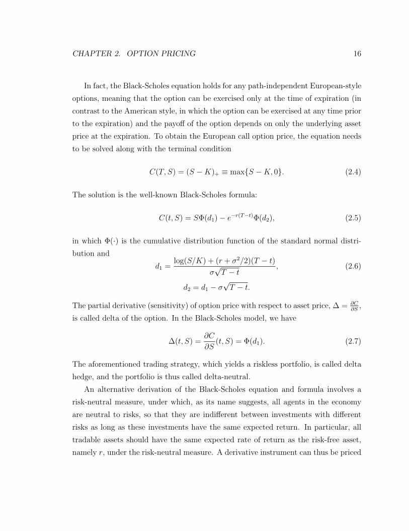
In fact, the Black-Scholes equation holds for any path-independent European-style
options, meaning that the option can be exercised only at the time of expiration (in
contrast to the American style, in which the option can be exercised at any time prior
to the expiration) and the payoff of the option depends on only the underlying asset
price at the expiration. To obtain the European call option price, the equation needs
to be solved along with the terminal condition
C(T, S) = (S −K)+ ≡ max{S −K, 0}. (2.4)
The solution is the well-known Black-Scholes formula:
C(t, S) = SΦ(d1)− e−r(T−t)Φ(d2), (2.5)
in which Φ(·) is the cumulative distribution function of the standard normal distri-
bution and
d1 =log(S/K) + (r + σ2/2)(T − t)
σ√T − t
, (2.6)
d2 = d1 − σ√T − t.
The partial derivative (sensitivity) of option price with respect to asset price, ∆ = ∂C∂S
,
is called delta of the option. In the Black-Scholes model, we have
∆(t, S) =∂C
∂S(t, S) = Φ(d1). (2.7)
The aforementioned trading strategy, which yields a riskless portfolio, is called delta
hedge, and the portfolio is thus called delta-neutral.
An alternative derivation of the Black-Scholes equation and formula involves a
risk-neutral measure, under which, as its name suggests, all agents in the economy
are neutral to risks, so that they are indifferent between investments with different
risks as long as these investments have the same expected return. In particular, all
tradable assets should have the same expected rate of return as the risk-free asset,
namely r, under the risk-neutral measure. A derivative instrument can thus be priced

CHAPTER 2. OPTION PRICING 17
by simply taking its expected payoff, discounted back to the current time at the risk-
free rate r. It can be shown that, in the absence of arbitrage opportunities, there exists
a unique risk-neutral measure in a complete market, where all tradable assets can be
replicated by a set of fundamental assets (the fundamental theorem of arbitrage). For
a European call option, by risk-neutral pricing we have
C(t, St) = e−r(T−t)EQ [(ST −K)+] , (2.8)
in which EQ[·] means taking expectation under the risk-neutral measure Q. This leads
to the same Black-Scholes formula (2.5) by using the fact that the asset price St is
still a geometric Brownian motion with the growth rate µ replaced by r under the
risk-neutral measure. The Feynman-Kac formula generalizes the relation between the
risk neutral pricing (2.8) and the Black-Scholes equation (2.3).
2.1.2 Jump Diffusion Model
To explain the empirical pattern of stock price series that far too many large price
movements are observed for the constant-volatility log-normal distribution in the
Black-Scholes theory, Merton (1976) proposes the following jump diffusion model,
which incorporates discontinuities in asset returns:
dSt/St = [µ− λ(m− 1)]dt+ σdWt + (Yt − 1)dNt, (2.9)
where
1. Wt is a standard Brownian motion;
2. Nt , the number of jumps that have occurred up to time t, is a Poisson process
with constant intensity λ, independent of Wt;
3. µ is the instantaneous expected asset return conditional on no jumps;
4. σ is the instantaneous volatility of asset price conditional on no jumps;
CHAPTER 2. OPTION PRICING 18
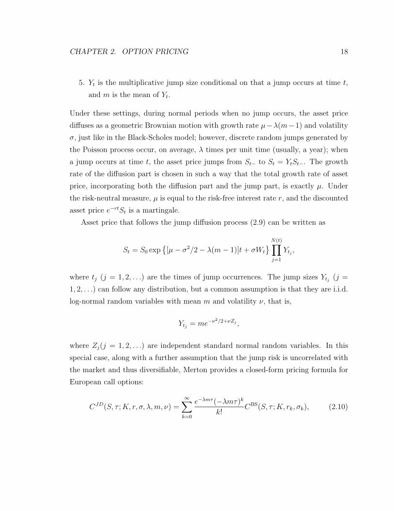
5. Yt is the multiplicative jump size conditional on that a jump occurs at time t,
and m is the mean of Yt.
Under these settings, during normal periods when no jump occurs, the asset price
diffuses as a geometric Brownian motion with growth rate µ−λ(m−1) and volatility
σ, just like in the Black-Scholes model; however, discrete random jumps generated by
the Poisson process occur, on average, λ times per unit time (usually, a year); when
a jump occurs at time t, the asset price jumps from St− to St = YtSt−. The growth
rate of the diffusion part is chosen in such a way that the total growth rate of asset
price, incorporating both the diffusion part and the jump part, is exactly µ. Under
the risk-neutral measure, µ is equal to the risk-free interest rate r, and the discounted
asset price e−rtSt is a martingale.
Asset price that follows the jump diffusion process (2.9) can be written as
St = S0 exp{
[µ− σ2/2− λ(m− 1)]t+ σWt
}N(t)∏j=1
Ytj ,
where tj (j = 1, 2, . . .) are the times of jump occurrences. The jump sizes Ytj (j =
1, 2, . . .) can follow any distribution, but a common assumption is that they are i.i.d.
log-normal random variables with mean m and volatility ν, that is,
Ytj = me−ν2/2+νZj ,
where Zj(j = 1, 2, . . .) are independent standard normal random variables. In this
special case, along with a further assumption that the jump risk is uncorrelated with
the market and thus diversifiable, Merton provides a closed-form pricing formula for
European call options:
CJD(S, τ ;K, r, σ, λ,m, ν) =∞∑k=0
e−λmτ (−λmτ)k
k!CBS(S, τ ;K, rk, σk), (2.10)

CHAPTER 2. OPTION PRICING 19
where τ = T − t is time to expiration, CBS(S, τ ;K, rk, σk) is the Black-Scholes price
(2.5) when the risk-free rate is
rk = r − λ(m− 1) +k log(m)
τ
and the volatility is
σk =
√σ2 +
kν2
τ.
Merton also points out that the trading strategy using
∆JD(S, τ ;K, r, σ, λ,m, ν) =∞∑k=0
e−λmτ (−λmτ)k
k!∆BS(S, τ ;K, rk, σk) (2.11)
shares of the underlying asset, where ∆BS(S, τ ;K, rk, σk) is the Black-Scholes delta
(2.7) with risk-free rate rk and volatility σk, cannot eliminate the jump risk, but it
does eliminate all systematic risk, and in that sense, is a hedge.
2.2 A Semiparametric Approach
Nonparametric methods for option pricing begin with the work of Hutchinson, Lo
and Poggio (1994) on European call options. They use a “learning network”, which is
trained from historical data on option prices, to provide an option pricing formula as
a function of an input vector x consisting of time to expiration T − t and moneyness
S/K. Three kinds of networks are considered:
1. radial basis function (RBF) networks
f(x) = β0 + µTx+I∑i=1
βihi(‖A(x− γi)‖),
where A is a positive definite matrix and hi is of the RBF type e−y2/σ2
i or
(y2 + σ2i )
1/2;
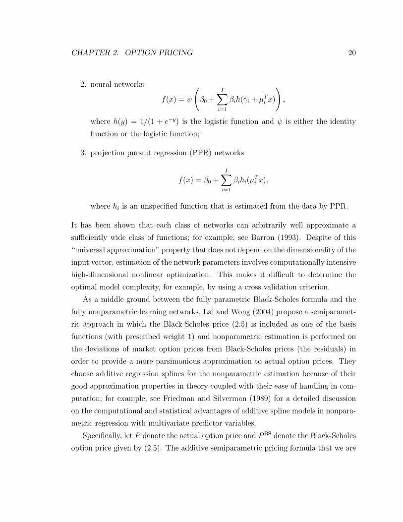
CHAPTER 2. OPTION PRICING 20
2. neural networks
f(x) = ψ
(β0 +
I∑i=1
βih(γi + µTi x)
),
where h(y) = 1/(1 + e−y) is the logistic function and ψ is either the identity
function or the logistic function;
3. projection pursuit regression (PPR) networks
f(x) = β0 +I∑i=1
βihi(µTi x),
where hi is an unspecified function that is estimated from the data by PPR.
It has been shown that each class of networks can arbitrarily well approximate a
sufficiently wide class of functions; for example, see Barron (1993). Despite of this
“universal approximation” property that does not depend on the dimensionality of the
input vector, estimation of the network parameters involves computationally intensive
high-dimensional nonlinear optimization. This makes it difficult to determine the
optimal model complexity, for example, by using a cross validation criterion.
As a middle ground between the fully parametric Black-Scholes formula and the
fully nonparametric learning networks, Lai and Wong (2004) propose a semiparamet-
ric approach in which the Black-Scholes price (2.5) is included as one of the basis
functions (with prescribed weight 1) and nonparametric estimation is performed on
the deviations of market option prices from Black-Scholes prices (the residuals) in
order to provide a more parsimonious approximation to actual option prices. They
choose additive regression splines for the nonparametric estimation because of their
good approximation properties in theory coupled with their ease of handling in com-
putation; for example, see Friedman and Silverman (1989) for a detailed discussion
on the computational and statistical advantages of additive spline models in nonpara-
metric regression with multivariate predictor variables.
Specifically, let P denote the actual option price and PBS denote the Black-Scholes
option price given by (2.5). The additive semiparametric pricing formula that we are
CHAPTER 2. OPTION PRICING 21
going to use hereafter is given by
P = PBS +Keρu (a0 + f1(u) + f2(z)) , (2.12)
where u = σ2(T − t) and z = log(er(T−t)S/K) are the two predictor variables, ρ =
−r/σ2, f1 and f2 are cubic splines in their respective inputs, for which the truncated-
power basis representations are
f1(u) = a1u+ a2u2 + a3u
3 +Ju∑j=1
a3+j(u− u(j)
)3+,
f2(z) = b1z + b2z2 + b3z
3 +Jz∑j=1
b3+j(z − z(j)
)3+,
which are piecewise cubic functions that have continuous first and second derivatives
at the knots u(j) and z(j). Here aj and bj are regression parameters that need to
be estimated from the training sample. Predictor u is variance of log return of the
asset from the current time to the expiration, and predictor z is log moneyness of
the option, defined as the ratio of the forward asset price to the strike. The choice
of these two predictor variables are motivated by rewriting the Black-Scholes formula
(2.5) asC(u, z)
Keρu= ezΦ
(z + u/2
u1/2
)− Φ
(z − u/2u1/2
),
the right-hand side of which does not involve any parameters that need to be exoge-
nously specified. In the original work of Lai and Wong, an additional cubic spline
function of w = u−1/2(z − u/2), an “interaction” variable derived from u and z, is
also used. We decide to drop this additional term because it causes wild behavior
of the pricing formula when the option gets close to its expiration (u is small and w
is large) and the simulation study has not shown its significance in the pricing for-
mula. Furthermore, we have increased the smoothness of the original pricing formula
in Lai and Wong (2004) by replacing quadratic splines with cubic splines, consid-
ering that second-order sensitivities (e.g., gamma, the second derivative of option
price with respect to asset price) are often interesting in option pricing and hedging

CHAPTER 2. OPTION PRICING 22
as well. For computational savings, the knots u(j) and z(j) are restricted to be the
100(j − 1/2)/Ju-th (j = 1, . . . , Ju) and 100(j − 1/2)/Jz-th (j = 1, . . . , Jz) percentiles
of the observations {u1, . . . , un} and {z1, . . . , zn} of the training sample, with the
numbers of knots Ju and Jz each chosen from all the possible integers between 0 and
10. When Ju and Jz are fixed in advance, the parameters aj and bj of the regression
splines can be estimated by least-squares, giving rise to a linear fitting method. As
a result, the optimal model complexity parameters Ju and Jz are selected so as to
minimize the generalized cross validation (GCV) criterion, which can be expressed in
the following form:
GCV(Ju, Jz) =1
n
n∑i=1
(Pi − Pi
1− (Ju + Jz + 7)/n
)2
, (2.13)
where Pi and Pi denote the i-th observed and fitted option price, respectively. The
final estimated pricing formula P is the one corresponding to the optimal choices of
Ju and Jz. By taking the derivative of the pricing formula with respect to asset price,
the option delta can then be estimated by
∆ = ∆BS + e−zf ′2(z),
where ∆BS is the Black-Scholes delta (2.7).
Although this semiparametric approach is first introduced by Lai and Wong (2004)
in order to estimate the “early exercise premium”, which is the difference between
the price of an American option and the price of its European counterpart, we have
generalized this approach to estimate the deviation of the actual option price from a
benchmark model price. This is helpful when models for the underlying asset price
dynamics do not work well in practice, or a closed-form pricing formula is difficult
to obtain due to the complexity of the asset price model while a relatively simple
benchmark model is available and can explain the empirical data to a reasonable
extent. Furthermore, besides the much lower computational complexity of using linear
least-squares and the simple GCV criterion, another advantage of the semiparametric
approach is that the time-variation of interest rate r and volatility σ is incorporated
CHAPTER 2. OPTION PRICING 23
by the inclusion of the Black-Scholes price as a basis function and our choice of the
predictor variables, while these two parameters are simply assumed to be constant
in both the learning networks of Hutchinson, Lo and Poggio (1994) and the kernel
smoothers of Aıt-Sahalia and Lo (1998) and Broadie, Detemple, Ghysels and Torres
(2000).
2.3 A Simulation Study
In this section, we present the results of a simulation study examining the performance
of the semiparametric pricing approach when the true underlying asset price dynamics
is known to follow Merton’s jump diffusion process.
2.3.1 Generating the Data
Following the simulation study in Hutchinson, Lo and Poggio (1994) on the perfor-
mance of learning-network pricing of European call options, we generate under the
risk-neutral measure 10 two-year samples of daily stock prices from the discretized
jump diffusion process
Snδ = S0 exp
{n∑i=1
(Xi + IiZi)
},
where δ = 1/252 is the step size of time-discretization in the unit of year (assuming 252
trading days per year), by drawing 504 i.i.d. normal random variables Xi with mean
(r − σ2/2)/252 and variance σ2/252, Bernoulli random variables Ii that take value 1
with probability 1− e−λδ and normal random variables Zi with mean log(m)− ν2/2and variance ν2, Xi, Ii and Zi being independent of each other. We use the following
values of the parameters: S0 = $50, r = 5%, σ = 25%, λ = 1, m = 90% and ν = 25%.
Therefore, on average, one jump in the stock price occurs every year, and a jump cuts
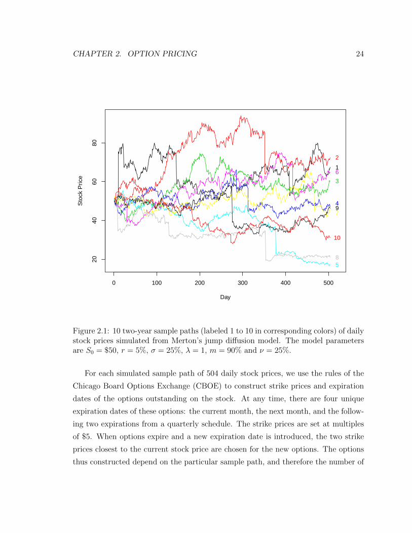
down the stock price by 10%. Figure 2.1 displays the 10 two-year sample paths of
daily stock prices thus simulated. Among the 10 sample, four contain one jump, four
contain two jumps, and two contain four jumps.
CHAPTER 2. OPTION PRICING 24
0 100 200 300 400 500
2040
6080
Day
Sto
ck P
rice
1
2
3
4
5
6
7
8
9
10
Figure 2.1: 10 two-year sample paths (labeled 1 to 10 in corresponding colors) of dailystock prices simulated from Merton’s jump diffusion model. The model parametersare S0 = $50, r = 5%, σ = 25%, λ = 1, m = 90% and ν = 25%.
For each simulated sample path of 504 daily stock prices, we use the rules of the
Chicago Board Options Exchange (CBOE) to construct strike prices and expiration
dates of the options outstanding on the stock. At any time, there are four unique
expiration dates of these options: the current month, the next month, and the follow-
ing two expirations from a quarterly schedule. The strike prices are set at multiples
of $5. When options expire and a new expiration date is introduced, the two strike
prices closest to the current stock price are chosen for the new options. The options
thus constructed depend on the particular sample path, and therefore the number of

CHAPTER 2. OPTION PRICING 25
Table 2.1: Summary of regression statistics for fitting semiparametric formulas to the10 simulated training samples of option data. RMSE stands for root mean squareerror. J∗u and J∗z are the optimal numbers of basis functions in u and z, respectively.
Size RMSE R2 J∗u J∗zSample 1 7,824 0.1093 0.9997 10 2Sample 2 8,378 0.1227 0.9996 5 7Sample 3 7,091 0.0795 0.9998 8 10Sample 4 6,836 0.1142 0.9991 5 10Sample 5 6,744 0.0961 0.9993 10 2Sample 6 7,330 0.0968 0.9996 6 8Sample 7 6,721 0.0696 0.9997 7 9Sample 8 6,518 0.0965 0.9991 10 3Sample 9 6,161 0.1342 0.9984 10 6Sample 10 6,593 0.0796 0.9995 10 8
options and the total number of data points vary across sample paths. For our 10
simulated paths, the number of options ranges from 83 to 118, with an average of
98; the total number of data points ranges from 6, 202 to 8, 430, with an average of
7, 069. The option prices are given by (2.10).
2.3.2 Training Semiparametric Pricing Formulas
We fit the semiparametric pricing formula (2.12) to each of the 10 training samples.
Data points for which τ = 0 are excluded from the training samples because option
price is trivial and equal to (S−K)+ for these data points. For simplicity, we assume
that both r and σ are known and need not be estimated. The maximum numbers
of basis functions of the two predictor variables are Ju = Jz = 10, and the optimal
set of basis function are selected by minimizing the GCV criterion (2.13). Table 2.1
summarizes some of the regression statistics for each training sample.

CHAPTER 2. OPTION PRICING 26
2.3.3 Pricing Performance
When the estimated semiparametric pricing formula is used to predict option prices
for new data points, we need to be careful about the issue of extrapolation. Rigorously
speaking, the estimated pricing formula can only be used inside the convex hull
H = {(u, z) : 0 ≤ u ≤ umax, z(u) ≤ z ≤ z(u)}
of the training sample S, where umax = max{u : u ∈ S}, and z(·) and z(·) are
the lower and upper boundaries of the convex hull, respectively. For data points
outside H, we use the following hybrid method to do safer extrapolation and correct
the potential erratic behavior of polynomial basis functions near or outside the data
boundaries. Specifically, for a new data point (u, z), if u > umax, we simply use
P (u, z) = PBS(u, z); otherwise, for 0 ≤ u ≤ umax and z /∈ [z(u), z(u)], we use
P (u, z) =
w(u)P SP(u, z) + [1− w(u)]PBS(u, z) if z < z(u),
w(u)P SP(u, z) + [1− w(u)]PBS(u, z) if z > z(u),(2.14)
where P SP(·, ·) is the estimated semiparametric pricing formula, w(u) = ez−z(u) and
w(u) = ez(u)−z.
To assess the quality of the semiparametric pricing formula obtained from each
training sample, we simulate an independent six-month path of daily stock prices,
construct options along the path according to the CBOE rules, and use the fitted
pricing formula to predict the new option prices. Naturally, we use the root mean
square error (RMSE) of the predicted prices for all options in the test sample as
the pricing performance measure. By simulating many independent test paths, 500
in our case, and averaging the RMSE over these paths, we can obtain an estimate
of the expected RMSE for each of the 10 training samples. This averaged pricing
performance measure is then compared to the same performance measure given by
the Black-Scholes pricing formula; see the first column of Panel A in Table 2.2. Using
the semiparametric pricing formula can reduce 70% to 84% of the average RMSE
from using the Black-Scholes formula. Also reported is the fraction of all data points
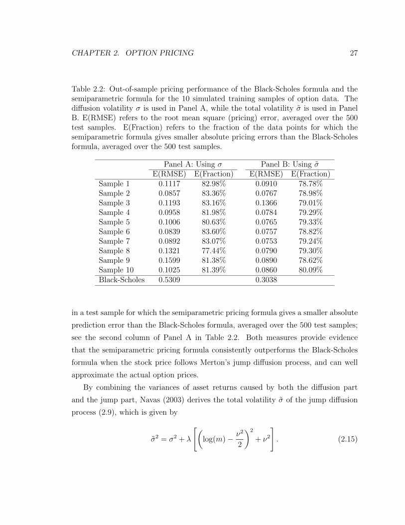
CHAPTER 2. OPTION PRICING 27
Table 2.2: Out-of-sample pricing performance of the Black-Scholes formula and thesemiparametric formula for the 10 simulated training samples of option data. Thediffusion volatility σ is used in Panel A, while the total volatility σ is used in PanelB. E(RMSE) refers to the root mean square (pricing) error, averaged over the 500test samples. E(Fraction) refers to the fraction of the data points for which thesemiparametric formula gives smaller absolute pricing errors than the Black-Scholesformula, averaged over the 500 test samples.
Panel A: Using σ Panel B: Using σE(RMSE) E(Fraction) E(RMSE) E(Fraction)
Sample 1 0.1117 82.98% 0.0910 78.78%Sample 2 0.0857 83.36% 0.0767 78.98%Sample 3 0.1193 83.16% 0.1366 79.01%Sample 4 0.0958 81.98% 0.0784 79.29%Sample 5 0.1006 80.63% 0.0765 79.33%Sample 6 0.0839 83.60% 0.0757 78.82%Sample 7 0.0892 83.07% 0.0753 79.24%Sample 8 0.1321 77.44% 0.0790 79.30%Sample 9 0.1599 81.38% 0.0890 78.62%Sample 10 0.1025 81.39% 0.0860 80.09%Black-Scholes 0.5309 0.3038
in a test sample for which the semiparametric pricing formula gives a smaller absolute
prediction error than the Black-Scholes formula, averaged over the 500 test samples;
see the second column of Panel A in Table 2.2. Both measures provide evidence
that the semiparametric pricing formula consistently outperforms the Black-Scholes
formula when the stock price follows Merton’s jump diffusion process, and can well
approximate the actual option prices.
By combining the variances of asset returns caused by both the diffusion part
and the jump part, Navas (2003) derives the total volatility σ of the jump diffusion
process (2.9), which is given by
σ2 = σ2 + λ
[(log(m)− ν2
2
)2
+ ν2
]. (2.15)
CHAPTER 2. OPTION PRICING 28
After replacing the diffusion volatility σ with the total volatility σ, which is equal
to 0.3790 in our case, we repeat the same procedure of training the semiparametric
pricing formula for each training sample and predicting the option prices in each test
sample. The same pricing performance measures are reported in Panel B of Table
2.2. Using the total volatility σ in place of the diffusion volatility σ does improve
the pricing performance for both the Black-Scholes formula and the semiparametric
formula, especially for the former. Nevertheless, the consistent advantage by using
the semiparametric formula over using the Black-Scholes formula is unchanged.
2.4 An Application to S&P 500 Futures Options
In the previous section, we have shown that the semiparametric approach can effi-
ciently approximate the jump diffusion pricing formula (2.10) if stock prices are gen-
erated by a jump diffusion process. To examine whether the semiparametric approach
is also useful in practice, we apply it to the pricing of S&P 500 futures options, and
compare it to the Black-Scholes model applied to the same data. S&P 500 futures op-
tions are among the most actively traded options available in the market. They have
been studied by Hutchinson, Lo and Poggio (1994), Bates (2000), Broadie, Chernov
and Johannes (2007), and a number of other authors.
2.4.1 The Data and Experimental Setup
The data for our empirical illustration are daily settlement prices of S&P 500 futures
and futures options for the 22-year period from December 1986 to December 2008,
obtained from the Chicago Mercantile Exchange (CME). We use the settlement prices
rather than the closing prices, which are used by Hutchinson, Lo and Poggio (1994),
as the former are used to calculate gains and losses in market accounts. The futures
contracts have quarterly expirations and expire on the third Friday of March, June,
September and December. For a quarterly option that expires in the March quarterly
cycle, the underlying futures contract is the one that expires in the same month as the
option does; for a serial option that expires in a month other than those in the March
CHAPTER 2. OPTION PRICING 29
quarterly cycle, which was first introduced in September 1987, the underlying futures
contract is the one that expires in the nearest month in the March quarterly cycle.
The expiration date of a quarterly option was initially the third Friday of the month,
same as its underlying futures contract, but was changed in the second quarter of
1986 to the day before due to concerns about the “triple witching hour”, which refers
to the last trading hour (3:00-4:00 p.m. EST) of that day, on which three kinds of
securities, namely stock market index futures, stock market index options and stock
options, all expire, resulting in extra trading volume and volatility of options, futures
and underlying stocks. Serial options still trade till the third Friday of their expiration
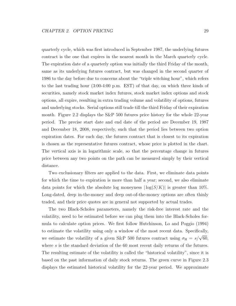
month. Figure 2.2 displays the S&P 500 futures price history for the whole 22-year
period. The precise start date and end date of the period are December 19, 1987
and December 18, 2008, respectively, such that the period lies between two option
expiration dates. For each day, the futures contract that is closest to its expiration
is chosen as the representative futures contract, whose price is plotted in the chart.
The vertical axis is in logarithmic scale, so that the percentage change in futures
price between any two points on the path can be measured simply by their vertical
distance.
Two exclusionary filters are applied to the data. First, we eliminate data points
for which the time to expiration is more than half a year; second, we also eliminate
data points for which the absolute log moneyness | log(S/K)| is greater than 10%.
Long-dated, deep in-the-money and deep out-of-the-money options are often thinly
traded, and their price quotes are in general not supported by actual trades.
The two Black-Scholes parameters, namely the risk-free interest rate and the
volatility, need to be estimated before we can plug them into the Black-Scholes for-
mula to calculate option prices. We first follow Hutchinson, Lo and Poggio (1994)
to estimate the volatility using only a window of the most recent data. Specifically,
we estimate the volatility of a given S&P 500 futures contract using σH = s/√
60,
where s is the standard deviation of the 60 most recent daily returns of the futures.
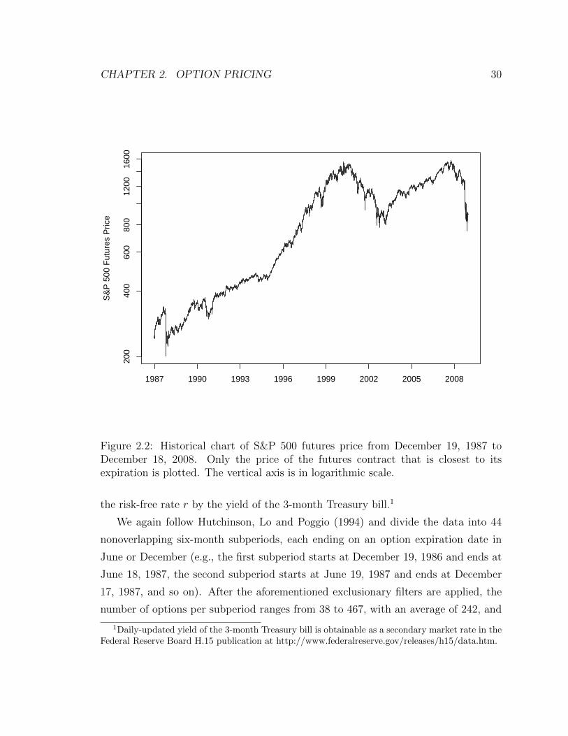
The resulting estimate of the volatility is called the “historical volatility”, since it is
based on the past information of daily stock returns. The green curve in Figure 2.3
displays the estimated historical volatility for the 22-year period. We approximate
CHAPTER 2. OPTION PRICING 30
200
400
600
800
1200
1600
S&
P 5
00 F
utur
es P
rice
1987 1990 1993 1996 1999 2002 2005 2008
Figure 2.2: Historical chart of S&P 500 futures price from December 19, 1987 toDecember 18, 2008. Only the price of the futures contract that is closest to itsexpiration is plotted. The vertical axis is in logarithmic scale.
the risk-free rate r by the yield of the 3-month Treasury bill.1
We again follow Hutchinson, Lo and Poggio (1994) and divide the data into 44
nonoverlapping six-month subperiods, each ending on an option expiration date in
June or December (e.g., the first subperiod starts at December 19, 1986 and ends at
June 18, 1987, the second subperiod starts at June 19, 1987 and ends at December
17, 1987, and so on). After the aforementioned exclusionary filters are applied, the
number of options per subperiod ranges from 38 to 467, with an average of 242, and
1Daily-updated yield of the 3-month Treasury bill is obtainable as a secondary market rate in theFederal Reserve Board H.15 publication at http://www.federalreserve.gov/releases/h15/data.htm.
CHAPTER 2. OPTION PRICING 31
0.0
0.2
0.4
0.6
0.8
Vol
atili
ty
1987 1990 1993 1996 1999 2002 2005 2008
Historical VolImplied VolCalibrated Vol
Figure 2.3: Historical volatility, at-the-money implied volatility and calibrated volatil-ity estimated from the S&P 500 futures option data for the period from December19, 1987 to December 18, 2008. Implied volatility is calculated for the option thathas the smallest absolute log moneyness among the options that are closest to theirexpiration dates.
the total number of data points per subperiod ranges from 2,573 to 21,170, with an
average of 11,280, both displaying an upward trend.
To limit the effects of nonstationarities and to avoid data-snooping, a separate
semiparametric pricing formula is estimated for each of the subperiods (except the
last one) and used to predict the option prices in the immediately following subperiod.
Same as in the simulation study, data points with time to expiration equal to 0 are
omitted for estimating the pricing formula, and the same correction (2.14) is used for
test data points that lie outside the convex hull of the training sample.
CHAPTER 2. OPTION PRICING 32
2.4.2 Pricing Performance
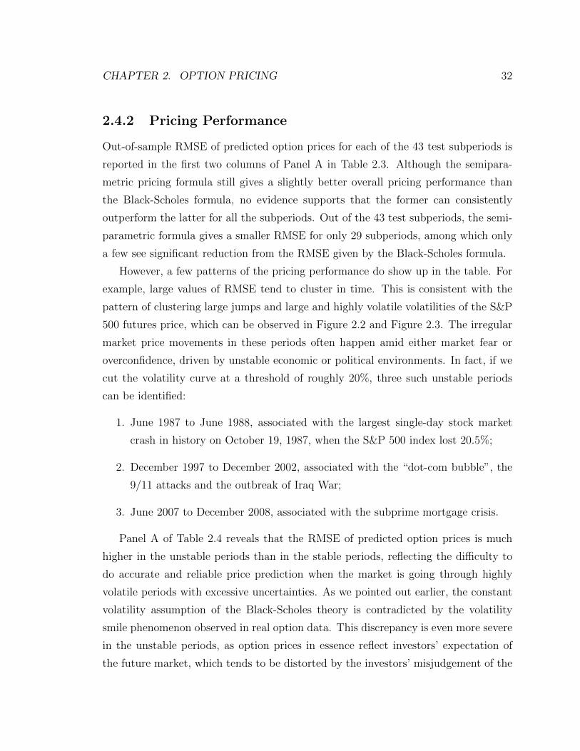
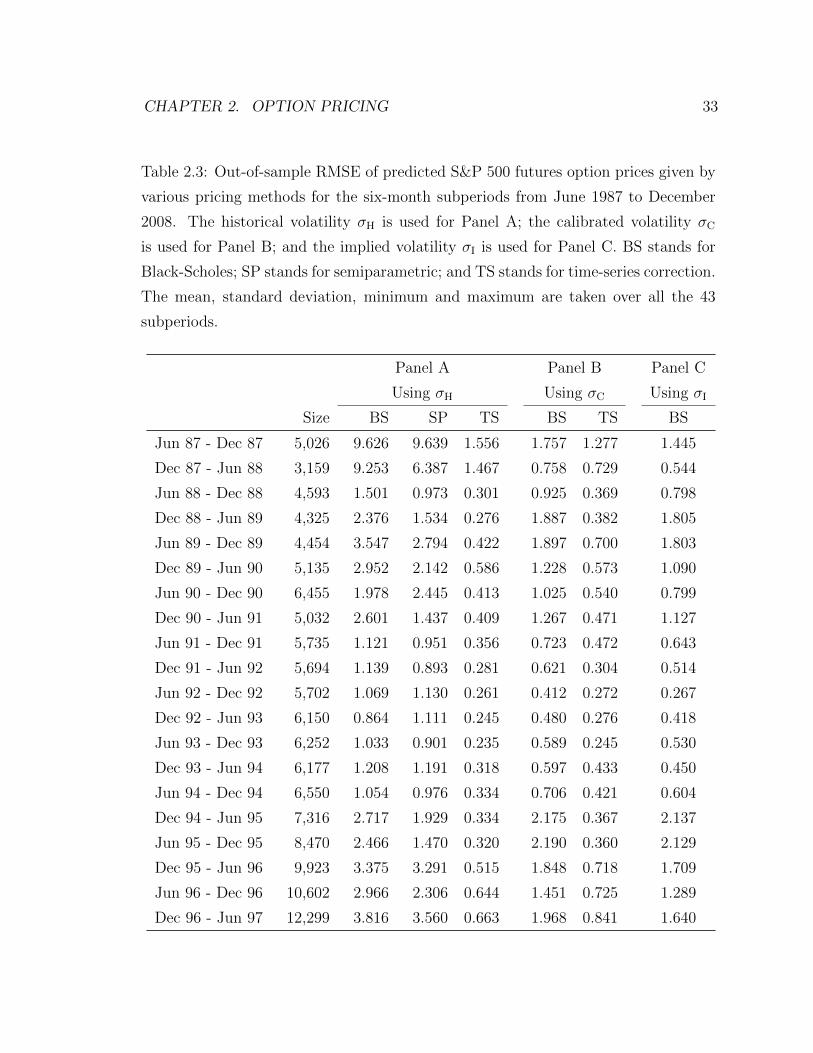
Out-of-sample RMSE of predicted option prices for each of the 43 test subperiods is
reported in the first two columns of Panel A in Table 2.3. Although the semipara-
metric pricing formula still gives a slightly better overall pricing performance than
the Black-Scholes formula, no evidence supports that the former can consistently
outperform the latter for all the subperiods. Out of the 43 test subperiods, the semi-
parametric formula gives a smaller RMSE for only 29 subperiods, among which only
a few see significant reduction from the RMSE given by the Black-Scholes formula.
However, a few patterns of the pricing performance do show up in the table. For
example, large values of RMSE tend to cluster in time. This is consistent with the
pattern of clustering large jumps and large and highly volatile volatilities of the S&P
500 futures price, which can be observed in Figure 2.2 and Figure 2.3. The irregular
market price movements in these periods often happen amid either market fear or
overconfidence, driven by unstable economic or political environments. In fact, if we
cut the volatility curve at a threshold of roughly 20%, three such unstable periods
can be identified:
1. June 1987 to June 1988, associated with the largest single-day stock market
crash in history on October 19, 1987, when the S&P 500 index lost 20.5%;
2. December 1997 to December 2002, associated with the “dot-com bubble”, the
9/11 attacks and the outbreak of Iraq War;
3. June 2007 to December 2008, associated with the subprime mortgage crisis.
Panel A of Table 2.4 reveals that the RMSE of predicted option prices is much
higher in the unstable periods than in the stable periods, reflecting the difficulty to
do accurate and reliable price prediction when the market is going through highly
volatile periods with excessive uncertainties. As we pointed out earlier, the constant
volatility assumption of the Black-Scholes theory is contradicted by the volatility
smile phenomenon observed in real option data. This discrepancy is even more severe
in the unstable periods, as option prices in essence reflect investors’ expectation of
the future market, which tends to be distorted by the investors’ misjudgement of the
CHAPTER 2. OPTION PRICING 33
Table 2.3: Out-of-sample RMSE of predicted S&P 500 futures option prices given by
various pricing methods for the six-month subperiods from June 1987 to December
2008. The historical volatility σH is used for Panel A; the calibrated volatility σC
is used for Panel B; and the implied volatility σI is used for Panel C. BS stands for
Black-Scholes; SP stands for semiparametric; and TS stands for time-series correction.
The mean, standard deviation, minimum and maximum are taken over all the 43
subperiods.
Panel A Panel B Panel C
Using σH Using σC Using σI
Size BS SP TS BS TS BS
Jun 87 - Dec 87 5,026 9.626 9.639 1.556 1.757 1.277 1.445
Dec 87 - Jun 88 3,159 9.253 6.387 1.467 0.758 0.729 0.544
Jun 88 - Dec 88 4,593 1.501 0.973 0.301 0.925 0.369 0.798
Dec 88 - Jun 89 4,325 2.376 1.534 0.276 1.887 0.382 1.805
Jun 89 - Dec 89 4,454 3.547 2.794 0.422 1.897 0.700 1.803
Dec 89 - Jun 90 5,135 2.952 2.142 0.586 1.228 0.573 1.090
Jun 90 - Dec 90 6,455 1.978 2.445 0.413 1.025 0.540 0.799
Dec 90 - Jun 91 5,032 2.601 1.437 0.409 1.267 0.471 1.127
Jun 91 - Dec 91 5,735 1.121 0.951 0.356 0.723 0.472 0.643
Dec 91 - Jun 92 5,694 1.139 0.893 0.281 0.621 0.304 0.514
Jun 92 - Dec 92 5,702 1.069 1.130 0.261 0.412 0.272 0.267
Dec 92 - Jun 93 6,150 0.864 1.111 0.245 0.480 0.276 0.418
Jun 93 - Dec 93 6,252 1.033 0.901 0.235 0.589 0.245 0.530
Dec 93 - Jun 94 6,177 1.208 1.191 0.318 0.597 0.433 0.450
Jun 94 - Dec 94 6,550 1.054 0.976 0.334 0.706 0.421 0.604
Dec 94 - Jun 95 7,316 2.717 1.929 0.334 2.175 0.367 2.137
Jun 95 - Dec 95 8,470 2.466 1.470 0.320 2.190 0.360 2.129
Dec 95 - Jun 96 9,923 3.375 3.291 0.515 1.848 0.718 1.709
Jun 96 - Dec 96 10,602 2.966 2.306 0.644 1.451 0.725 1.289
Dec 96 - Jun 97 12,299 3.816 3.560 0.663 1.968 0.841 1.640
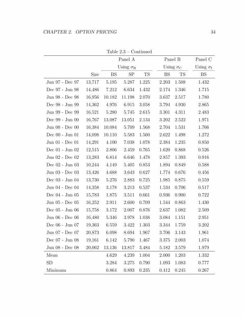
CHAPTER 2. OPTION PRICING 34
Table 2.3 – Continued
Panel A Panel B Panel C
Using σH Using σC Using σI
Size BS SP TS BS TS BS
Jun 97 - Dec 97 13,717 5.195 5.287 1.225 2.203 1.508 1.432
Dec 97 - Jun 98 14,486 7.212 6.634 1.432 2.174 1.346 1.715
Jun 98 - Dec 98 16,956 10.182 11.198 2.070 3.637 2.517 1.780
Dec 98 - Jun 99 14,362 4.976 6.915 3.058 3.794 4.930 2.865
Jun 99 - Dec 99 16,521 5.280 5.745 2.615 3.301 4.311 2.483
Dec 99 - Jun 00 16,767 13.087 13.051 2.134 3.202 2.522 1.971
Jun 00 - Dec 00 16,384 10.084 5.709 1.568 2.704 1.531 1.766
Dec 00 - Jun 01 14,098 10.110 5.583 1.560 2.622 1.498 1.272
Jun 01 - Dec 01 14,291 4.100 7.038 1.078 2.384 1.235 0.850
Dec 01 - Jun 02 12,515 2.806 2.459 0.765 1.620 0.868 0.526
Jun 02 - Dec 02 13,283 6.814 6.646 1.478 2.857 1.393 0.916
Dec 02 - Jun 03 10,244 4.149 5.405 0.853 1.894 0.849 0.588
Jun 03 - Dec 03 13,426 4.688 3.643 0.627 1.774 0.676 0.456
Dec 03 - Jun 04 13,730 5.276 2.883 0.725 1.985 0.875 0.559
Jun 04 - Dec 04 14,358 3.178 3.213 0.537 1.534 0.706 0.517
Dec 04 - Jun 05 15,783 1.875 3.511 0.661 0.936 0.900 0.722
Jun 05 - Dec 05 16,252 2.911 2.600 0.709 1.544 0.863 1.430
Dec 05 - Jun 06 15,758 3.172 2.007 0.876 2.637 1.082 2.509
Jun 06 - Dec 06 16,480 5.346 3.978 1.038 3.084 1.151 2.951
Dec 06 - Jun 07 19,363 6.559 3.422 1.303 3.344 1.759 3.202
Jun 07 - Dec 07 20,873 6.098 8.694 1.967 3.706 3.143 1.961
Dec 07 - Jun 08 19,161 6.142 5.790 1.467 3.375 2.003 1.074
Jun 08 - Dec 08 20,062 13.136 13.817 3.484 5.182 3.579 1.979
Mean 4.629 4.239 1.004 2.000 1.203 1.332
SD 3.284 3.275 0.790 1.093 1.083 0.777
Minimum 0.864 0.893 0.235 0.412 0.245 0.267
CHAPTER 2. OPTION PRICING 35
Table 2.3 – Continued
Panel A Panel B Panel C
Using σH Using σC Using σI
Size BS SP TS BS TS BS
Maximum 13.136 13.817 3.484 5.182 4.930 3.202
Overall 487,919 6.357 6.133 1.472 2.629 1.920 1.699
market instability that they are observing. For example, over-optimism and over-
pessimism may lead to overpriced in-the-money call options and overpriced in-the-
money put options (hence overpriced out-of-the-money call options), respectively. All
these increase the error when the Black-Scholes formula is used to predict the option
price. Since we use the Black-Scholes price as the benchmark and starting point in
our semiparametric pricing formula, the pricing performance of the semiparametric
formula is unavoidably adversely affected by the poor performance of the Black-
Scholes formula. On the other hand, in the stable periods, the semiparametric formula
does give improvement in pricing over the Black-Scholes formula, nevertheless the
improvement is limited, as the latter has already given a reasonably good estimate
for the option price. In summary, the semiparametric formula does not noticeably
outperform the Black-Scholes formula for the S&P 500 futures option data, contrary
to the conclusion of the simulation study in Section 2.3.
2.5 A Time-Series Approach
Although the empirical results in Section 2.4.2 are somewhat disappointing, it is too
early to jump to the conclusion that the semiparametric pricing approach completely
fails in practice. One natural and straightforward modification to the approach is
to choose a different length of the training and test subperiods. The success of a
statistical learning approach depends heavily on the stationarity of the data to which
it is applied. The semiparametric approach can succeed only when the underlying
distribution and characteristics of the data of the training period can be well extended
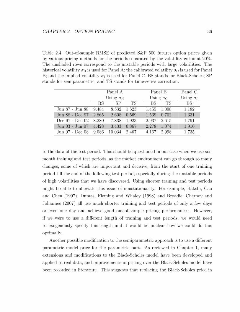
CHAPTER 2. OPTION PRICING 36
Table 2.4: Out-of-sample RMSE of predicted S&P 500 futures option prices givenby various pricing methods for the periods separated by the volatility cutpoint 20%.The unshaded rows correspond to the unstable periods with large volatilities. Thehistorical volatility σH is used for Panel A; the calibrated volatility σC is used for PanelB; and the implied volatility σI is used for Panel C. BS stands for Black-Scholes; SPstands for semiparametric; and TS stands for time-series correction.
Panel A Panel B Panel CUsing σH Using σC Using σI
BS SP TS BS TS BSJun 87 - Jun 88 9.484 8.532 1.523 1.455 1.098 1.182Jun 88 - Dec 97 2.865 2.608 0.569 1.539 0.702 1.331Dec 97 - Dec 02 8.280 7.838 1.923 2.937 2.615 1.791Jun 03 - Jun 07 4.428 3.433 0.867 2.278 1.074 1.916Jun 07 - Dec 08 9.086 10.034 2.467 4.167 2.998 1.735
to the data of the test period. This should be questioned in our case when we use six-
month training and test periods, as the market environment can go through so many
changes, some of which are important and decisive, from the start of one training
period till the end of the following test period, especially during the unstable periods
of high volatilities that we have discovered. Using shorter training and test periods
might be able to alleviate this issue of nonstationarity. For example, Bakshi, Cao
and Chen (1997), Dumas, Fleming and Whaley (1998) and Broadie, Chernov and
Johannes (2007) all use much shorter training and test periods of only a few days
or even one day and achieve good out-of-sample pricing performances. However,
if we were to use a different length of training and test periods, we would need
to exogenously specify this length and it would be unclear how we could do this
optimally.
Another possible modification to the semiparametric approach is to use a different
parametric model price for the parametric part. As reviewed in Chapter 1, many
extensions and modifications to the Black-Scholes model have been developed and
applied to real data, and improvements in pricing over the Black-Scholes model have
been recorded in literature. This suggests that replacing the Black-Scholes price in
CHAPTER 2. OPTION PRICING 37
the semiparametric pricing formula by one of the alternative models could improve
the pricing performance of the semiparametric approach as well. However, these
refined parametric models often have a relatively large number of parameters, whose
calibration to the real data involves high-dimensional optimization, which could be
computationally expensive and unstable. Furthermore, most of the empirical studies
in literature use short training and test periods of data for model calibration and out-
of-sample performance measurement. Whether these models can give comparably
good pricing performances for longer periods of data is unclear to us. This raises the
same issue of how to optimally determine the length of training and test periods.
So the question is: if we still use the Black-Scholes price for the parametric part
and do not want to worry about the choice of the subperiod length, can we modify the
semiparametric approach to improve its pricing performance? The only option left to
us is the nonparametric part, and we propose to model it using a time-series approach.
This is motivated by our findings from examining the autocorrelation function of the
series εt = Pt − PBSt , the difference between the market price and the Black-Scholes
price at time t (or, as we call it, the “residual”). Panel A of Table 2.5 summarizes the
autocorrelation coefficients of εt up to the 3rd lag. The extremely high autocorrela-
tions suggest using information extracted from the residuals of the previous days to
predict the residual of the current day. We carry out lag-1 autoregression of εt against
εt−1 and find an almost perfect fit; see Panel B of Table 2.5. In fact, excluding the
two subperiods in year 1999, the R2 always exceeds 0.878 and the regression coeffi-
cient is always larger than 0.922 for the remaining 42 subperiods; in other words, the
observed lag-1 residual pairs (εt−1, εt) almost always lie approximately on a straight
line whose slope is very close to 45◦.
Since the lag-1 autocorrelation is already very close to 1 and the lag-1 autoregres-
sion almost perfectly fits to the observed residuals, for simplicity, we propose to use
the following lag-1 correction for the Black-Scholes Price:
Pt = PBSt + εt−1
= PBSt + (Pt−1 − PBS
t−1). (2.16)
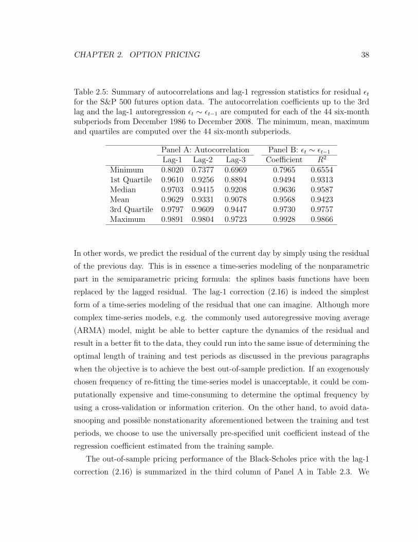
CHAPTER 2. OPTION PRICING 38
Table 2.5: Summary of autocorrelations and lag-1 regression statistics for residual εtfor the S&P 500 futures option data. The autocorrelation coefficients up to the 3rdlag and the lag-1 autoregression εt ∼ εt−1 are computed for each of the 44 six-monthsubperiods from December 1986 to December 2008. The minimum, mean, maximumand quartiles are computed over the 44 six-month subperiods.
Panel A: Autocorrelation Panel B: εt ∼ εt−1Lag-1 Lag-2 Lag-3 Coefficient R2
Minimum 0.8020 0.7377 0.6969 0.7965 0.65541st Quartile 0.9610 0.9256 0.8894 0.9494 0.9313Median 0.9703 0.9415 0.9208 0.9636 0.9587Mean 0.9629 0.9331 0.9078 0.9568 0.94233rd Quartile 0.9797 0.9609 0.9447 0.9730 0.9757Maximum 0.9891 0.9804 0.9723 0.9928 0.9866
In other words, we predict the residual of the current day by simply using the residual
of the previous day. This is in essence a time-series modeling of the nonparametric
part in the semiparametric pricing formula: the splines basis functions have been
replaced by the lagged residual. The lag-1 correction (2.16) is indeed the simplest
form of a time-series modeling of the residual that one can imagine. Although more
complex time-series models, e.g. the commonly used autoregressive moving average
(ARMA) model, might be able to better capture the dynamics of the residual and
result in a better fit to the data, they could run into the same issue of determining the
optimal length of training and test periods as discussed in the previous paragraphs
when the objective is to achieve the best out-of-sample prediction. If an exogenously
chosen frequency of re-fitting the time-series model is unacceptable, it could be com-
putationally expensive and time-consuming to determine the optimal frequency by
using a cross-validation or information criterion. On the other hand, to avoid data-
snooping and possible nonstationarity aforementioned between the training and test
periods, we choose to use the universally pre-specified unit coefficient instead of the
regression coefficient estimated from the training sample.
The out-of-sample pricing performance of the Black-Scholes price with the lag-1
correction (2.16) is summarized in the third column of Panel A in Table 2.3. We
CHAPTER 2. OPTION PRICING 39
can see that the time-series correction has achieved a remarkable improvement over
the uncorrected Black-Scholes price for every six-month test period. The percentage
reduction in RMSE of predicted option prices exceeds 64.52% for every test period
except the two in year 1999, which, as we mentioned earlier, have the smallest lag-1
autocorrelations of the residual among the 43 test periods; the percentage reduction in
RMSE for these two subperiods are 37.76% and 50.00%, respectively. The maximum
and mean of the percentage reduction in RMSE are 92.37% and 78.72%, respectively,
and the overall percentage reduction in RMSE for all the 43 test periods combined
is 76.29%. In Panel A of Table 2.4, the subperiods are grouped according to the
volatility cutpoint of 20%, and the corresponding RMSE of predicted option prices
given by the corrected Black-Scholes formula is reported in the third column. For
the two stable periods, the percentage reduction in RMSE from the uncorrected
Black-Scholes price are 80.12% and 80.41%, while for the three unstable periods,
the percentage reduction in RMSE are 83.94%, 76.77% and 72.85%. The time-series
correction results in comparable improvements over the Black-Scholes price for both
the stable periods and the unstable periods. As we expected, the simplest time-
series modeling of the nonparametric part in the semiparametric formula can already
efficiently improve the out-of-sample pricing performance for S&P 500 futures options.
2.5.1 Comparison with Implied Volatility Approaches
As a final comparison, we examine the out-of-sample pricing performance based on
the option’s implied volatility. The implied volatility σI is defined as the volatility
value that equates the Black-Scholes option price with the actual market option price,
that is, σI solves
P = CBS(S, τ ;K, r, σI), (2.17)
where P is the actual option price and CBS(S, τ ;K, r, σI) is the Black-Scholes price
(2.5) when the volatility is equal to σI. In the following we will use σI(t) to indicate
the time-dependence of the implied volatility.
To determine the current option price, what really matters is the future realization
of the underlying asset’s volatility. This can be easily explained by the risk-neutral

CHAPTER 2. OPTION PRICING 40
pricing formula (2.8). Therefore, using the implied volatility for option pricing does
make more sense than using the historical volatility, in that the latter is a backward
estimate using the past behavior of the underlying asset price to project the future,
while the former is by nature a forward estimate, noting that the expectation of mar-
ket participants on the future volatility is incorporated into the actual option price.
However, empirical studies have shown that the implied volatility not only varies with
time, but also depends on the option’s strike price and time to expiration. This makes
the idea somewhat self-contradictory to imply the volatility from the actual option
price using the Black-Scholes formula, as the formula holds only when the volatility
is a constant. Furthermore, it does not make sense that the volatility differs for each
individual option, since, by definition, the volatility is solely a characteristic of the
underlying asset. Nonetheless, the implied volatility is still worth a careful and seri-
ous examination, for it is simple to implement and is commonly adopted in practice,
and its efficiency in option pricing and hedging has been well recorded in literature.
A closely related estimate of the volatility is the one that is calibrated to the daily
cross-section of observed option prices instead of each individual option as the implied
volatility does. This “calibrated volatility” σC is defined as the minimizer of the sum
of squared differences between the market option prices and the Black-Scholes prices:
σC = arg minσ≥0.01
n∑i=1
[Pi − CBS(S, τi;Ki, r, σ)
]2,
where the summation is taken over all options in the cross-section, indexed by i. A
minimum value 0.01 is imposed to prevent negative values of the estimated volatility.
In the following we will use σC(t) to indicate the time-dependence of the calibrated
volatility. This volatility estimate is one of the smoothed implied volatility functions
examined by Dumas, Fleming and Whaley (1998), and is shown to be the best es-
timate for hedging by their empirical study on S&P 500 index options. Although it
has a relatively poor pricing performance compared to the volatility function which
is quadratic in strike price, it is more comparable to the historical volatility estimate
in that the property is preserved that it does not vary across options, which complies
with the original definition of volatility. We choose to examine this estimate as well so
CHAPTER 2. OPTION PRICING 41
that we can compare the pricing performances among different contract-independent
volatility estimates.
It turns out that Equation (2.17) does not always have a positive solution for the
S&P 500 futures option data. This is in theory impossible. The Black-Scholes formula
(2.5) is an increasing continuous function of σ, whose lower limit is the no-arbitrage
lower bound of the option price implied from the put-call parity2 as σ approaches 0
and upper limit is the underlying asset price, which trivially dominates the option
price, as σ approaches infinity. Therefore, in the absence of arbitrage opportunities,
a positive solution to Equation (2.17) should always exist. However, several factors
may cause the implied volatility to not exist in practice:
1. The observed option price is not supported by an actual trade, so that the price
quote is out-of-date. This can happen for thinly traded long-dated options or
options far from the money.
2. The option price and the underlying asset price are not quoted concurrently,
which actually happens all the time, as the two instruments are traded inde-
pendently in different markets. However, this imperfect synchronization is often
negligible when the two prices are quoted very close in time.
3. The risk-free rate r and hence the lower limit of the Black-Scholes price, S −e−rτK, are overestimated. This can happen for options with less than 3 months
to expire, since we are using the 3-month Treasury bill rate as a proxy for r and
a yield curve usually has positive slope. As a cure, for each individual option,
one can use the point on the yield curve that corresponds to its expiration,
but this approach is again self-contradictory like the implied-volatility, as the
Black-Scholes model assumes a contract-independent constant risk-free rate.
When the implied volatility σI does not exist for an option, we use the calibrated
volatility σC of the same day as a proxy for σI.
2The put-call parity says that the relationship C − P = S −KB(T ) holds at any time prior toT . Here C and P are the prices of the European call and put options with the same strike price Kand expiration T , S is the stock price, and B(T ) is the price of the zero-coupon bond with maturityT and a unit face value. This relationship can be proved by a no-arbitrage argument, noting thatboth sides correspond to two portfolios that have the same payoff at time T .
CHAPTER 2. OPTION PRICING 42
In Figure 2.3, the dashed red curve and the solid black curve correspond to the
estimated implied volatility and calibrated volatility, respectively, for S&P 500 futures
options over the 22-year period from December 1986 to December 2008. These two
curves lie quite close to each other; a large proportion of the two curves are not even
distinguishable under the displayed resolution. However, the implied volatility curve
appears more volatile when large movements of the volatility occur. For example, the
implied volatility shoots up to around 90% in October 1987 when the stock market
crash happens, while the peak of the calibrated volatility is only around 60% during
that period. This is not surprising since the latter is smoothed out when calibrated to
the whole daily cross-section of option prices instead of each individual option price.
Both show remarkable deviation from the historical volatility curve.
Now, for any day in the 22-year period, we estimate the option prices on that day
by plugging the previous day’s calibrated volatility into the Black-Scholes formula
(2.5). In other words, we use the estimate σC(t) = σC(t − δ), where δ is the time
step size, which, in our case, is one day. The RMSE of predicted option prices for
each six-month test period is reported in the first column of Panel B in Table 2.3.
This approach outperforms using the Black-Scholes price with the historical volatility
for every six-month test period. The reduction in RMSE ranges from 11.20% to
91.81%, with an average of 49.42%. The overall RMSE for all the 43 six-month
periods combined is reduced by 58.56%. Panel B of Table 2.4 summarizes the RMSE
for the grouped subperiods. For the three unstable periods, using the calibrated
volatility achieves RMSE reductions of 84.66%, 64.53% and 54.13%, respectively,
while for the two stable periods, the reductions in RMSE are only 46.28% and 48.56%,
respectively. The effect of using the calibrated volatility is more remarkable for the
unstable periods, in which the Black-Scholes price with the historical volatility suffers
a big failure. What surprises us is that the first unstable period from June 1987 to
June 1988 has an even smaller RMSE than the two stable periods. In fact, Table 2.4
does suggest that the RMSE has an upward trend in time. This is probably because
more and more options with different strike prices and expirations are traded in the
market, making it increasingly difficult to accurately price all of them using the Black-
Scholes formula with a single global volatility. Similar to the previous results for the
CHAPTER 2. OPTION PRICING 43
historical volatility, the semiparametric pricing formula does not give a noticeably
better performance than the Black-Scholes formula when the calibrated volatility is
used instead, and thus the results are not reported.
Also reported in Panel B of Table 2.3 is the RMSE of predicted option prices
given by the lag-1 corrected Black-Scholes price (2.16) using σC for each of the six-
month test periods. Excluding the two test periods in year 1999, the lag-1 correction
improves the pricing performance for all the remaining 41 test periods; the percentage
reduction in RMSE ranges from 3.78% to 83.56%, with an average of 46.48%. This
is much less impressive than the lag-1 correction for the Black-Scholes price using
the historical volatility σH. In fact, across the 44 six-month subperiods, the lag-1
autocorrelation of the residual εt for the Black-Scholes price using σC ranges from
0.1319 to 0.9886, with an average of 0.8294, which is in general much lower than
the lag-1 autocorrelation of εt for the Black-Scholes price using σH; see Panel A of
Table 2.5. Furthermore, the coefficient for the lag-1 autoregression of εt ranges from
0.1406 to 0.9847, with an average of 0.7994, which in general differs from 1 by a large
margin. This suggests that the lag-1 correction sometimes overcorrects the Black-
Scholes price in this case. Compared with the lag-1 corrected Black-Scholes price
using σH, using σC gives a better pricing performance for only 8 out of the 43 test
periods. This finding is quite the opposite to the result of the comparison between
the uncorrected Black-Scholes prices using σH and σC, in which the latter easily beats
the former. A time-series model more complex than the simple lagging of εt might be
needed to achieve a better times-series correction to the Black-Scholes price using σC.
Again, the corresponding RMSE of predicted option prices for the grouped subperiods
is reported in Panel B of Table 2.4. With the lag-1 correction applied, the pricing
performance is again much better for the stable periods than for the unstable periods.
Finally, as commonly practiced in industry, for any day and any option traded on
that day, we estimate the option price by plugging the previous day’s volatility implied
from the same option into the Black-Scholes formula (2.5). In other words, we use the
estimate σI(t) = σI(t− δ). The last column of Table 2.3 and Table 2.4 summarize the
resulting RMSE of predicted option prices for each six-month subperiod and grouped
subperiod, respectively. Overall speaking, the Black-Scholes price using σI gives the
CHAPTER 2. OPTION PRICING 44
most stable pricing performance over all the 43 six-month subperiods in the sense that
the maximum and the standard deviation of its RMSE are the smallest among all
the pricing approaches. Its performance does not differ much between the stable and
unstable periods. The only competitor is the lag-1 corrected Black-Scholes price using
σH, outperforming the Black-Scholes pricing using σI for 26 out of the 43 six-month
subperiods and achieving a 13.36% reduction in overall RMSE from the latter. When
σI is used, both the semiparametric approach and the time-series correction give only
similar or sometimes even worse pricing performances compared to the Black-Scholes
price because of the same reason as discussed for the calibrated volatility, and thus
the results are not reported.
The great improvement in pricing performance by using the calibrated or implied
volatility in the Black-Scholes formula over using the historical volatility might suggest
the importance of choosing a good volatility estimate. The calibrated and implied
volatilities win because their estimation involves both the underlying asset price data
and the option price data, while only the former is used to estimate the historical
volatility. With this in mind, we are not surprised to see that using the calibrated
or implied volatility has such a huge advantage in predicting future option prices,
as information contained in option prices is already incorporated in these volatility
estimates. One step further, the success of these pricing approaches lends support to
the idea of more general time-series modeling of the option price. In fact, our time-
series corrected Black-Scholes price is very similar by nature to using the previous
day’s calibrated or implied volatility in the sense that both correct the Black-Scholes
price with parameters estimated from the previous day’s option data. The difference
is that, for the time-series corrected Black-Scholes price, the correction is applied
additively outside the Black-Scholes formula, while for the calibrated and implied
volatility approaches, the correction is applied inside the Black-Scholes formula in a
nonlinear way.
CHAPTER 2. OPTION PRICING 45
2.6 Conclusion
The semiparametric pricing approach initially proposed by Lai and Wong (2004) has
proven to perform well as expected in our simulation study using data sets generated
from Merton’s jump diffusion model. However, its application to the S&P 500 futures
and futures options suggests that this is not necessarily true in practice, especially
when the assumption of stationarity between the training and test periods breaks
down during an unstable period featuring a highly volatile market. The time-series
approach that we have proposed can be regarded as a new type of semiparamet-
ric approach, in which time-series modeling of the nonparametric part has replaced
the original additive regression splines. A simple additive lag-1 correction term can
already give an outstanding pricing performance for S&P 500 futures options, even
compared with the commonly favored Black-Scholes price using the implied volatility.
Taking into account that the implied volatility is relatively computationally expen-
sive to find and sometimes does not even exist, our time-series correction approach
provides a competitive alternative for accurate prediction of option prices.
Chapter 3
Option Hedging with Transaction
Costs
A key assumption in the derivation of the closed-form pricing formula for the Black-
Scholes model (or more generally, any deterministic volatility function models) is that
trading the underlying asset does not incur transaction costs of any forms. If this
assumption had broken down, then, for example, the dynamics of the gain process
for the Black-Scholes delta hedging strategy (2.2) would not hold without transac-
tion costs included, and hence the derivation could not proceed any further to arrive
at the Black-Scholes equation (2.3). In the real world, two facts have invalidated
this assumption: the existence of transaction costs and the infeasibility of continuous
hedging. Although the latter can be acceptably approximated by using sufficiently
short revision intervals, doing so will be disastrous, however, as more frequent rebal-
ancing means that more transaction costs are accumulated. In the following, we will
focus on transaction costs that are proportional to the value of trade. That is, if at
some time we buy y units of the underlying asset at price S, then a transaction cost
of amount λbyS needs to be paid aside from the payment yS for this purchase; here
λb is a constant independent of the trade volume y. Similarly, if the same order is
for sale instead, then we need to pay a transaction cost at a constant rate λs, or a
total amount of λsyS. This type of transaction costs is most commonly studied in
literature, and can well approximate the real transaction costs for a liquidly traded
46
CHAPTER 3. OPTION HEDGING WITH TRANSACTION COSTS 47
asset when the trade volume is negligible compared to the total volume of the asset
outstanding on the market.
This chapter is organized as follows. Sections 3.1 and 3.2 provide brief introduc-
tions to two different types of approaches to option hedging with transaction costs,
namely (i) discrete-time delta hedging using a modified volatility and (ii) singular
stochastic control problems that seek an optimal balance between the cost and the
risk of hedging an option. In Section 3.3, we propose a data-driven rule-based strat-
egy to connect the theoretical approaches with real-world applications. Similar to the
optimal solutions to the singular stochastic control problems, the rule-based strategy
is characterized by a pair of buy/sell boundaries and a no-transaction region in be-
tween. Details of criteria and a two-stage iterative procedure are provided for tuning
the boundaries to a long period of option data. The simulation studies in Section
3.4 compare the rule-based strategy with existing delta-hedging and optimal-control
strategies in terms of both the risk-cost tradeoff, a generalization of the risk-return
framework popular in the portfolio theory, for individual options and the overall hedg-
ing performance for all options within a long period. The practical usefulness of the
rule-based strategy is then assessed by an application to the S&P 500 futures option
data in Section 3.5. Favorable comparison results are obtained in both the simulation
studies and the empirical study, even though a very simple form of the boundaries
is used for the rule-based strategy. Making use of a reverting pattern observed in
the S&P 500 futures data, we refine the rule-based strategy by allowing hedging
suspension at large jumps in futures price. A more complex form of the rule-based
strategy for categorized options are also examined and compared with the simpler
form. Section 3.6 concludes this chapter.
3.1 Discrete-Time Replication
Continuous hedging assumed in the Black-Scholes theory is not feasible in the real
world, as a gap of at least milliseconds has to exist between two consecutive trans-
actions due to apparent reasons. A discrete-time approximation always replaces the
continuous hedging in practice. Suppose that we build a hedging portfolio at time 0
CHAPTER 3. OPTION HEDGING WITH TRANSACTION COSTS 48
for a European call option with strike price K and need to unwind our positions at
the expiration T of the option, and that we rebalance the portfolio at fixed equispaced
time points 0 < δ < 2δ < · · · < Nδ = T . The underlying stock price St follows the
geometric Brownian motion (2.1). Although the Black-Scholes delta hedging strategy
using ∆(t, St) (see (2.7)) shares of the stock will result in a nonzero random hedging
error at the expiration T due to the time-discretization, it can be shown that this
error vanishes as the revision interval length δ approaches 0. However, in the presence
of proportional transaction costs, the total amount of costs will rise as the revision
intervals become shorter and hence more transactions are executed. In fact, the total
transaction cost is not bounded because of the infinite total variation of a Brownian
motion. It may be very difficult to assure a given degree of replication accuracy before
an unaffordable amount of transaction costs is reached.
Leland (1985) proposes a modified Black-Scholes delta hedging strategy that per-
mits the replication of a short option position with a finite total amount of transaction
costs no matter how small δ is. At each revision time t, the hedging portfolio is ad-
justed by holding
∆L(t, St) = ∆(t, St;σL)
shares of the stock, where ∆(·, ·;σL) is the Black-Scholes delta (2.7) in which the
modified volatility
σL = σL(σ, δ, λb, λs) = σ
(1 +
λb + λs
σ
√2
πδ
)1/2
(3.1)
is used. It can be easily verified that, as δ goes to 0, the modified volatility becomes
infinity and this strategy is tantamount to the trivial static super-replicating strategy
in which a single share of the stock is held to hedge the option.
Leland claims that following this modified delta hedging strategy will yield the
payoff (2.4) of the option at the expiration inclusive of transaction costs as δ ap-
proaches 0. Unfortunately, his claim turns out to be flawed by the fact that the
hedging portfolio thus-constructed is not self-financing. However, intuitive interpre-
tations do lend some support to Leland’s idea of modifying the volatility. For hedging
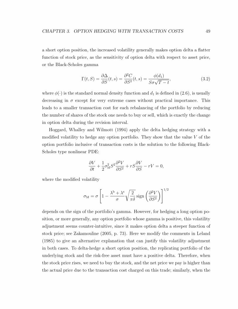
CHAPTER 3. OPTION HEDGING WITH TRANSACTION COSTS 49
a short option position, the increased volatility generally makes option delta a flatter
function of stock price, as the sensitivity of option delta with respect to asset price,
or the Black-Scholes gamma
Γ(t, S) =∂∆
∂S(t, s) =
∂2C
∂S2(t, s) =
φ(d1)
Sσ√T − t
, (3.2)
where φ(·) is the standard normal density function and d1 is defined in (2.6), is usually
decreasing in σ except for very extreme cases without practical importance. This
leads to a smaller transaction cost for each rebalancing of the portfolio by reducing
the number of shares of the stock one needs to buy or sell, which is exactly the change
in option delta during the revision interval.
Hoggard, Whalley and Wilmott (1994) apply the delta hedging strategy with a
modified volatility to hedge any option portfolio. They show that the value V of the
option portfolio inclusive of transaction costs is the solution to the following Black-
Scholes type nonlinear PDE:
∂V
∂t+
1
2σ2MS
2∂2V
∂S2+ rS
∂V
∂S− rV = 0,
where the modified volatility
σM = σ
[1− λb + λs
σ
√2
πδsign
(∂2V
∂S2
)]1/2
depends on the sign of the portfolio’s gamma. However, for hedging a long option po-
sition, or more generally, any option portfolio whose gamma is positive, this volatility
adjustment seems counter-intuitive, since it makes option delta a steeper function of
stock price; see Zakamouline (2005, p. 73). Here we modify the comments in Leland
(1985) to give an alternative explanation that can justify this volatility adjustment
in both cases. To delta-hedge a short option position, the replicating portfolio of the
underlying stock and the risk-free asset must have a positive delta. Therefore, when
the stock price rises, we need to buy the stock, and the net price we pay is higher than
the actual price due to the transaction cost charged on this trade; similarly, when the
CHAPTER 3. OPTION HEDGING WITH TRANSACTION COSTS 50
stock price drops, we need to sell the stock, and the net price we earn is lower than
the actual price. This amplification of stock price movements can be modeled as if
the volatility of the stock was higher than it actually is. Analogously, to delta-hedge a
long option position, the replicating portfolio must have a negative delta. Therefore,
when the stock price rises, the net price of selling the stock is lower than the actual
price; when the stock price drops, the net price of buying the stock is higher than
the actual price. This shrinkage of stock price movements can be modeled as if the
volatility of the stock was lower than it actually is.
3.2 Singular Stochastic Controls
Suppose that an investor is presented with an opportunity to enter into a short
position in the European call option with strike price K and expiration T . The
underlying stock price follows the geometric Brownian motion (2.1). There also exists
a risk-free asset which pays at a constant interest rate r. Suppose that, at any time
t prior to T , the investor has xt dollars invested in the risk-free asset and holds yt
shares of the stock. The dynamics of the investor’s position (xt, yt) in the stock and
the risk-free asset are given by
dxt = rxtdt− αStdLt + βStdMt, (3.3)
dyt = dLt − dMt (equivalently, yt = Lt −Mt),
where α = 1 + λb, β = 1− λs, and (Lt,Mt) is a non-decreasing and non-anticipating
processes such that Lt (resp. Mt) denotes the cumulative number of shares of the
stock bought (resp. sold) within the time interval [0, t]. When the investor does not
hold a position in the option, his/her terminal wealth after liquidating the stock is
V 0(xT , yT , ST ), where
V 0(x, y, S) = x+ yS(α1{x<0} + β1{x≥0}).
CHAPTER 3. OPTION HEDGING WITH TRANSACTION COSTS 51
For simplicity, we might sometimes assume that no transaction costs are charged at
time T . In this case, the above equation can be simplified as
V 0(x, y, S) = x+ yS.
When the investor holds a short option position, and if the option is cash-settled,
his/her terminal wealth after liquidating the stock is V w(xT , yT , ST ), where
V w(x, y, S) = V 0(x, y, S) + (S −K)+; (3.4)
if the option is asset-settled instead, then the terminal wealth function is
V w(x, y, S) = V 0(x, y − 1{S>K}, S) +K1{S>K}. (3.5)
Two singular stochastic control approaches have been proposed to find optimal option
hedging strategies under criteria depending on the hedger’s terminal wealth.
3.2.1 Utility Maximization
In the presence of proportional transaction costs, since a riskless hedging portfolio
of the underlying stock and the risk-free asset is no longer constructible, the option
hedger faces a tradeoff between the risk and the cost of hedging the option. There-
fore, in pricing and hedging the option, one must take into account the hedger’s risk
preference, which, in common sense, differs among individuals. In economics, a util-
ity function, which depends on a person’s risk preference, is often used to measure
the person’s relative satisfaction from any amount of money. The expected utility
theory states that people behave and make decisions as if they were maximizing the
expectation of the utility function of all possible outcomes. Hodges and Neuberger
(1989) pioneer the research on option pricing and hedging based on this theory.
Suppose that U : R→ R is the hedger’s utility function, which is usually concave
and increasing to reflect that the hedger is risk-averse. The goal is to maximize the
expected utility of the hedger’s terminal wealth by controlling the cumulative stock
CHAPTER 3. OPTION HEDGING WITH TRANSACTION COSTS 52
purchase process L and sale process M , or equivalently, the hedger’s stock holding
yt. Denote the hedger’s value function by
J i(t, x, y, S) = supL,M
E[U(V i(xT , yT , ST )
)∣∣xt = x, yt = y, St = S], (3.6)
where i = 0, w correspond to no option position and a short option position, respec-
tively. Although there is no closed-form solution to the stochastic control problem
(3.6), the existence and uniqueness of the solution is rigorously proved by Davis, Panas
and Zariphopoulou (1993). They also develop a discrete-time dynamic programming
scheme, which involves a backward induction on a 3-dimensional state-space tree.
When the negative exponential utility function
U(v) = 1− e−γv, (3.7)
where γ is a measure of the hedger’s risk aversion, is assumed, the optimal strategy
does not depend on the hedger’s position in the risk-free asset xt, one dimension
thus being reduced from the dynamic programming procedure. Refined discretization
schemes have been proposed by Clewlow and Hodges (1997) and Zakamouline (2006).
Let yit (i = 0, w) denote the optimal trading strategies for an investor with (i = w)
and without (i = 0) a short option position. Under the risk-neutral assumption µ = r,
it can be shown that y0t ≡ 0, that is, without the option liability, the investor will
choose not to invest in the stock at all. The optimal hedging strategy for the option
writer, who holds a short option position, is given by ywt − y0t . The “reservation
(selling) price” of the option is defined as the amount of cash P required initially
by the option writer to maintain the same expected utility of terminal wealth as not
selling the option. Mathematically, P satisfies
Jw(0, x+ P, y, S) = J0(0, x, y, S).
In other words, the reservation price of the option is such that makes the investor
indifferent between investing with and without entering a short option position.
Numerical computation shows that the optimal strategy y∗t for hedging the option

CHAPTER 3. OPTION HEDGING WITH TRANSACTION COSTS 53
is constrained to evolve between two boundaries Y b < Y s. As long as the hedger’s
stock holding lies between these two boundaries, no rebalancing of the hedging port-
folio is needed. The region between these two boundaries is therefore called the
“no-transaction region”. At the moment the hedger’s stock holding falls out of the
no-transaction region, he/she needs to rebalance the hedging portfolio in order to
return to the nearest boundary of the no-transaction region. Specifically, if y∗t moves
below Y b, the hedger needs to immediately buy the stock to bring it back to Y b; if
y∗t moves above Y s, the hedger needs to immediately sell the stock to bring it back
to Y s. The solid curves in Figure 3.1 provide an illustration for the boundaries of the
no-transaction region for µ = r = 0, σ = 0.3, T − t = 0.25, K = 100, λb = λs = 0.01
and γ = 0.6. The boundaries are not symmetric around the Black-Scholes delta,
which is also displayed in Figure 3.1 as the dotted curve. Assuming that λb = λs = λ
are sufficiently small, Whalley and Wilmott (1997) derive a closed-form expression
for the asymptotic boundaries of the no-transaction region:
Y b,s = ∆∓(
3e−r(T−t)λSΓ2
2γ
)1/3
,
where ∆ is the Black-Scholes delta (2.7) and Γ is the Black-Scholes gamma (3.2).
3.2.2 Cost-Constrained Risk Minimization
The total hedging cost incurred over the time interval [t, T ] is defined as the cu-
mulative interest-compounded costs for buying the stock and proceeds (regarded as
negative costs) from selling the stock or unwinding the option position at the expira-
tion. For hedging a short option position, this quantity is given by
C(L,M ; t, T ) = α
∫ T
t
er(T−u)SudLu − β∫ T
t
er(T−u)SudMu − (V w(xT , yT , ST )− xT ) .
(3.8)
Integrating (3.3) after multiplying both sides by er(T−t), we have
xT − xter(T−t) = −α∫ T
t
er(T−u)SudLu + β
∫ T
t
er(T−u)SudMu.
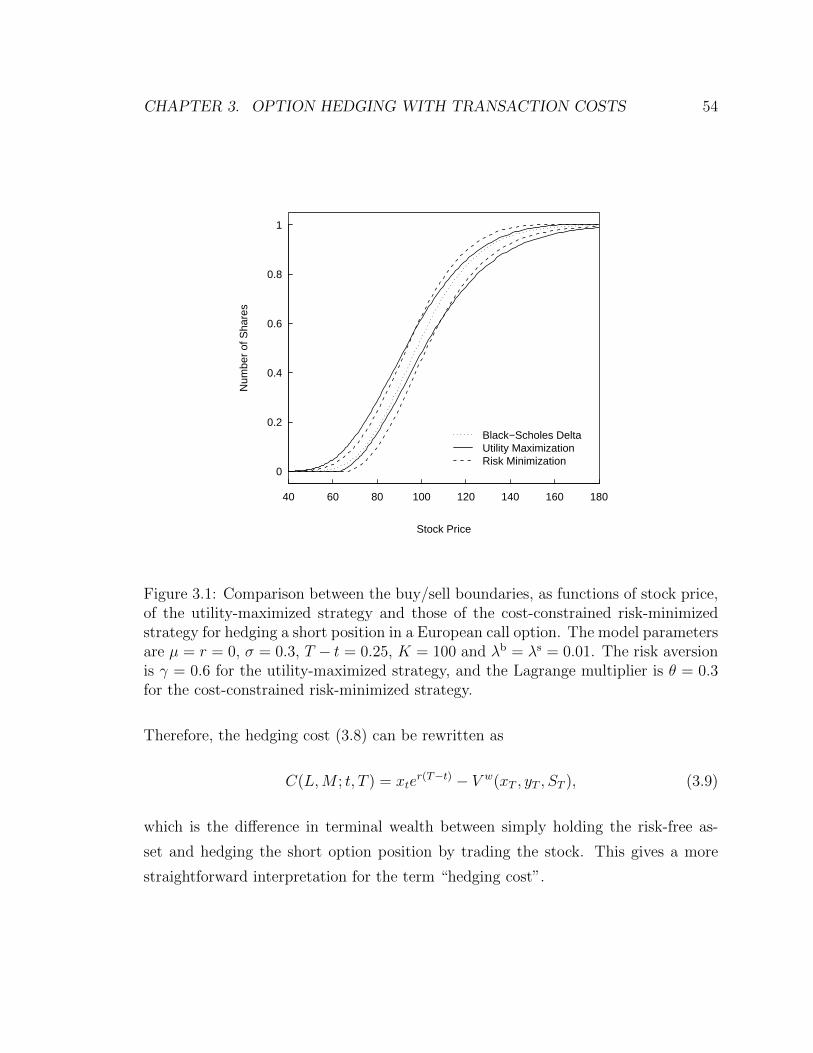
CHAPTER 3. OPTION HEDGING WITH TRANSACTION COSTS 54
Stock Price
Num
ber
of S
hare
s
40 60 80 100 120 140 160 180
0
0.2
0.4
0.6
0.8
1
Black−Scholes DeltaUtility MaximizationRisk Minimization
Figure 3.1: Comparison between the buy/sell boundaries, as functions of stock price,of the utility-maximized strategy and those of the cost-constrained risk-minimizedstrategy for hedging a short position in a European call option. The model parametersare µ = r = 0, σ = 0.3, T − t = 0.25, K = 100 and λb = λs = 0.01. The risk aversionis γ = 0.6 for the utility-maximized strategy, and the Lagrange multiplier is θ = 0.3for the cost-constrained risk-minimized strategy.
Therefore, the hedging cost (3.8) can be rewritten as
C(L,M ; t, T ) = xter(T−t) − V w(xT , yT , ST ), (3.9)
which is the difference in terminal wealth between simply holding the risk-free as-
set and hedging the short option position by trading the stock. This gives a more
straightforward interpretation for the term “hedging cost”.
CHAPTER 3. OPTION HEDGING WITH TRANSACTION COSTS 55
It has been shown that the direct minimization of the expected hedging cost
minL,M
E [C(L,M ; t, T )| yt = y, St = S] (3.10)
yields a trivial hedging strategy, in which the hedger does not need to do anything
before the expiration, or in other words, the option is not hedged at all. The failure
of (3.10) to produce a meaningful hedging strategy is due to the fact that it does
not address the riskiness of the hedging portfolio. A reasonable modification is to
also take into account the variance of the hedging cost, which leads to the following
variance-constrained cost minimization problem:
minL,M{E [C(L,M ; t, T )| yt = y, St = S] + ωVar [C(L,M ; t, T )| yt = y, St = S]} ,
(3.11)
where the Lagrange multiplier ω serves as a risk-aversion parameter; a larger value
of ω corresponds to a more risk-averse hedger.
However, the stochastic control problem associated with (3.11) is prohibitively
difficult to solve. This prompts Lai and Lim (2009) to use an alternative risk measure
rather than the variance of the hedging cost. They propose the following pathwise
risk over the time interval [t, T ]:
R(L,M ; t, T ) =
∫ T
t
σ2S2u [yu −∆(u, Su)]
2 du, (3.12)
where ∆(·, ·) is the Black-Scholes delta (2.7). It can be shown by a simple application
of Ito’s formula that the integrand in (3.12) is the instantaneous variance of the return
of the hedging portfolio. Therefore, R(L,M ; t, T ) is the “cumulative instantaneous
variance” of the hedging portfolio, and, in this sense, can serve well as a measure of
the hedging risk. In the absence of transaction costs, the Black-Scholes theory says
that the instantaneous variance of the return of the hedging portfolio can be made
exactly zero for any time t prior to T and for every realized path of the stock price
by continuously rebalancing to yt = ∆(t, St) shares of the stock.
Replacing the variance of the hedging cost with the pathwise risk (3.11), Lai
CHAPTER 3. OPTION HEDGING WITH TRANSACTION COSTS 56
and Lim formulate a risk-constrained cost minimization problem. They consider the
associated dual problem of the cost-constrained minimization of the pathwise risk,
for which the value function is given by
J(t, y, S) = infL,M
E [θR(L,M ; t, T ) + C(L,M ; t, T )| yt = y, St = S] , (3.13)
where the Lagrange multiplier 1/θ serves as a risk-aversion parameter; a larger value
of θ corresponds to a more risk-averse hedger. In the absence of transaction costs,
the expected terminal value of any self-financing hedging portfolio is always equal to
0, which implies a constant expected hedging cost. Therefore, (3.13) reduces to the
minimization of the expected pathwise risk in this case. The solution to this reduced
problem is obviously the Black-Scholes delta hedging strategy, at which the minimum
0 is attained. In this sense, the cost-constrained risk minimization problem provides
a natural extension of the Black-Scholes theory in the presence of transaction costs.
After a proper change of variables, Lai and Lim show that the partial derivative
of the value function (3.13) of the cost-constrained risk minimization problem with
respect to the stock holding y is the value function of an optimal stopping problem
associated with a Dynkin game, which in turn is the solution to a PDE with free
boundary conditions. A backward induction algorithm is provided to solve this free
boundary problem (FBP), and the value function (3.13) can then be obtained by
integration and an inverse change of variables. Lai and Lim also show that, although
the utility maximization problem cannot be reduced to an optimal stopping prob-
lem, the same technique can still be applied to establish a connection between its
value function and the solution to a FBP for an optimal stopping problem associated
with a Dynkin game. They provide a modified coupled backward induction algo-
rithm to iteratively solve for both the value function and its partial derivative with
respect to the stock holding. This algorithm is much simpler than the ones devel-
oped by Davis, Panas and Zariphopoulou (1993), Clewlow and Hodges (1997) and
Zakamouline (2006), which have to perform an additional nonlinear maximization to
identify the optimal trade size at each time step. Technical details are omitted here
and interested readers are referred to their paper.
CHAPTER 3. OPTION HEDGING WITH TRANSACTION COSTS 57
The optimal hedging strategy corresponding to the solution to (3.13) has features
similar to those of the utility-maximized hedging strategy. Specifically, when the
stock holding lies within the no-transaction region defined by the two boundaries
Y b < Y s, then the hedger simply maintains his/her positions and does nothing;
when the stock holding falls out of the no-transaction region, the hedger needs to
immediately rebalance his/her hedging portfolio to bring the stock holding back to
the nearest boundary. The dashed curves in Figure 3.1 display the boundaries of the
no-transaction region for the cost-constrained risk-minimized strategy for the same
values of the parameters as in Section 3.2.1 and the Lagrange multiplier θ = 0.3. The
boundaries are much more symmetric around the Black-Scholes delta than those of
the no-transaction region for the utility-maximized strategy.
3.3 Rule-Based Hedging Strategy
Although Section 3.2 provided approaches to finding the optimal hedging strate-
gies under two different but related criteria, namely utility maximization and cost-
constrained risk minimization, they both share some drawbacks that restrict their
applicability for real option data:
1. The optimal hedging strategy works only in a Black-Scholes world.
2. A multi-dimensional dynamic programming has to be performed to find the
optimal hedging strategy numerically.
3. The optimal hedging strategy is option-specific, so that a separate dynamic
programming has to be performed to find the optimal hedging strategy for each
individual option, which further increases the computational complexity.
4. The risk-aversion parameter λ or the Lagrange multiplier θ has to be exoge-
nously determined by the hedger’s risk preference, which is difficult to measure
in reality.
5. For the utility maximization approach, efficient dynamic programming schemes
have been developed only for the negative exponential utility function (3.7).
CHAPTER 3. OPTION HEDGING WITH TRANSACTION COSTS 58
All these drawbacks prompt us to find an alternative approach to option hedging with
transaction costs, which should be simpler to implement and more widely applicable
to different options under fewer assumptions on the stock price dynamics.
The semiparametric approach to option pricing has enlightened us on how to
establish a connection between the theoretical approaches and the real-world appli-
cation. The idea is to make correction to a benchmark theoretical hedging strategy
so as to achieve the best empirical hedging performance. Note that both the utility
maximization approach and the cost-constrained risk minimization approach yield
the optimal hedging strategies in a rigorous sense, that is, the strategies are indeed
optimal among all self-financing hedging strategies under their respective criteria.
However, in order to achieve a lower computational complexity and a more general
applicability, we have to sacrifice this rigorous optimality. Instead we will try to
achieve a sub-optimality in the sense that our hedging strategy is optimal among a
subclass of self-financing hedging strategies. In other words, we will first define a set
of rules for the feasible self-financing hedging strategies, and then find the optimal
one among these rule-based hedging strategies.
3.3.1 Buy/Sell Boundaries
Both the utility-maximized strategy and the cost-constrained risk-minimized strategy
can be characterized by a pair of buy/sell boundaries, defining a no-transaction region
within which the option hedger does not need to do anything. The distance between
the two boundaries reflects a tradeoff between the hedging risk and the hedging
cost. When the no-transaction region between the two boundaries is narrow, the
rebalancing of the hedging portfolio tends to occur more frequently, resulting in a
lower hedging risk and a higher hedging cost; conversely, when the no-transaction
region is wide, the rebalancing of the hedging portfolio occurs less frequently, resulting
in a higher hedging risk and a lower hedging cost. Intuitively, in the presence of
transaction costs, one should slow down the hedging to reduce the hedging cost, and
should rebalance his/her portfolio only when it is necessary to keep the hedging risk
from rising to an intolerable level.

CHAPTER 3. OPTION HEDGING WITH TRANSACTION COSTS 59
Now suppose that an investor needs to hedge a short position in a European
call option with strike price K and expiration T by holding an offsetting position
in the underlying stock. Rebalancing of the hedging portfolio can occur only at
discrete time points 0 < δ < 2δ < · · · < Nδ = T . Let yt denote the number
of shares of the stock that the hedger holds at any time t prior to T . Motivated
by the utility-maximized strategy and the cost-constrained risk-minimized strategy,
our first rule of the feasible hedging strategies is that there exists a pair of buy/sell
boundaries, such that the hedger rebalances the hedging portfolio only when his/her
stock holding falls out of the no-transaction region between these two boundaries, and
when that happens, the hedger buys or sells the stock to bring his/her stock holding
back to the nearest boundary. Furthermore, we assume that the hedging strategies are
Markovian, and hence that the boundaries are functions of time t and stock price St
only. Mathematically, there exists a pair of buy/sell boundaries Y b(t, S) < Y s(t, S),
such that
ynδ =
Y b(nδ, Snδ) if y(n−1)δ < Y b(nδ, Snδ),
y(n−1)δ if Y b(nδ, Snδ) ≤ y(n−1)δ ≤ Y s(nδ, Snδ),
Y s(nδ, Snδ) if y(n−1)δ > Y s(nδ, Snδ)
(3.14)
for n = 1, 2, . . . , N . There are infinitely many choices of Y b,s(·, ·). For example, both
the utility-maximized strategy and the cost-constrained risk-minimized strategy are
special cases of (3.14) when they are applied in discrete time; (3.14) is also tantamount
to the Black-Scholes delta hedging strategy or the Leland’s strategy in Section 3.1
when Y b(t, S) = Y s(t, S), both equal to ∆BS(t, S;σ) or ∆BS(t, S;σL), respectively,
where ∆BS is the Black-Scholes delta function (2.7) and σL is the modified volatility
(3.1).
We propose to use the following form of the buy/sell boundaries:
Y b(t, S) = max{
∆BS(t, S)− db(t, S), 0},
Y s(t, S) = min{
∆BS(t, S) + ds(t, S), 1},
(3.15)
CHAPTER 3. OPTION HEDGING WITH TRANSACTION COSTS 60
where db,s(·, ·) are two functions that always take positive values. Here we list a few
reasons behind our choice of this form of the boundaries:
1. As documented by many authors, in the absence of transaction costs, the Black-
Scholes delta hedging strategy performs sufficiently well compared to other
single-instrument (using only the stock) hedging strategies given by more com-
plex models; see, e.g., Dumas, Fleming and Whaley (1998) and Bakshi, Cao
and Chen (1997). Therefore, it can serve as a good benchmark hedging strat-
egy when transaction costs are taken into account.
2. Figure 3.1 suggests that we can well approximate the buy/sell boundaries of
the cost-constrained risk-minimized strategy by vertical displacements of the
Black-Scholes delta (not in a rigorous sense, as the size of each displacement
varies with the horizontal location), and those of the utility-maximized strategy
by vertical displacements of a flatter delta curve. The boundaries (3.15) share
the same property.
3. The boundaries should always lie between 0 and 1, since a long position in the
stock is required for hedging a short option position, and a single share of the
stock already super-replicates the option.
The form (3.15) of the boundaries incorporates (i) a benchmark hedging strategy
derived from a parametric option pricing model and (ii) a deviation of the strategy
from the benchmark strategy, which is to be statistically learned from option data by
using the criterion that we will discuss below. It is therefore similar by nature to the
semiparametric option pricing approach in Section 2.2. To estimate the deviation, a
functional form needs to be chosen for db,s(t, S), like the cubic regression splines in
the semiparametric pricing formula (2.12). For computational simplicity, the simplest
form
db(t, S) = ds(t, S) = d, (3.16)
where d is a positive constant, will be used for illustrative purpose in the following
simulation and empirical studies.
CHAPTER 3. OPTION HEDGING WITH TRANSACTION COSTS 61
3.3.2 Hedging Performance Measures
Following the notations in Section 3.2, we denote the risk-free asset value by xt and
the number of shares of the stock by yt for any time t prior to the expiration T of the
option. Suppose that there is no initial endowment at time 0 (before the option is
sold) and that the hedging portfolio is self-financing. Let Pt denote the option price
and
Vt = xt + ytSt − Pt
the value of the hedging portfolio at time t. Then V0 = 0 and the hedger’s terminal
wealth is VT = V w(xT , yT , ST ), where V w is defined by (3.4) if the option is cash-
settled or (3.5) if the option is asset-settled. VT is also called the “tracking error” by
Hutchinson, Lo and Poggio (1994). In the absence of transaction costs, the tracking
error can be made arbitrarily small by letting δ approach 0. The discrete-time version
of (3.3) can be written as
xnδ = x(n−1)δernδδ − αSnδ(ynδ − y(n−1)δ)+ + βSnδ(y(n−1)δ − ynδ)+
for n = 1, 2, . . . , N , where rt is the time-varying risk-free interest rate.
One way to assess the performance of a hedging strategy is to use the present
value of the root mean square tracking error
η = e−∫ T0 rtdt
√E(V 2
T ), (3.17)
which is called the “prediction error” by Hutchinson, Lo and Poggio. Note that, under
the assumption that the risk-free rate is constant or deterministic, it follows from
(3.9) that the total hedging cost over the time interval [0, T ] differs from the negative
tracking error −VT by only an additive constant. Therefore, the minimization of
the prediction error (3.17) is essentially quite close to the variance-constrained cost
minimization (3.11) in Section 3.2.2 in the sense that they both aim for a balance
between the expectation and the variance of the tracking error, except for the fact
that the risk-aversion is fixed and not variable in (3.17). Lai and Lim (2009, p.
1959) have shown a similar equivalence between minimizing the prediction error η

CHAPTER 3. OPTION HEDGING WITH TRANSACTION COSTS 62
and minimizing E(C2) − aE(C), where C = C(L,M ; 0, T ) is the total hedging cost
over the time interval [0, T ] and a = 2P0
∫ T0rtdt is a positive constant. This is in turn
tantamount to the Markowitz-type problem of minimizing Var(C) subject to a target
value of E(C), or equivalently, the variance-constrained cost minimization problem
(3.11).
3.3.3 Practical Implementation
In order to make use of the buy/sell boundaries (3.15), we need to estimate db,s(t, S)
from the data by optimizing some hedging performance measure. In particular, if
db,s(t, S) are given by (3.16), an appropriate value of d needs to be determined. The
expectation in (3.17) is taken under the physical probability measure over all possible
realizations of the stock price path over the time interval [0, T ]. Unfortunately, it is
impossible to observe or even give a good estimate for this expectation in practice,
since only one realization of the stock price path can be observed. Some might argue
that we could estimate this expectation by bootstrapping over the stock price path,
which involves sampling from the distribution of the stock return at each time step.
This sounds promising when we can easily obtain or estimate the distribution of the
stock return, e.g., in a simulation study where this distribution is actually known to us.
However, this becomes extremely difficult to carry out in practice, one major reason
being that the distribution of the stock return is highly likely to be nonstationary
over time and be influenced by time-series effects, such that it is unclear how one can
estimate an empirical distribution from the observed stock returns.
Now that estimating η for each individual option seems unrealistic, we propose the
following work-around to pool together a basket of options that we are interested in
and approximate η by an empirical analog. Suppose that there are M options in the
basket written on the same stock, indexed by m = 1, 2, . . . ,M . The time of initiation
and the time of expiration of the m-th option are denoted by tm and Tm, respectively.
We propose to approximate η by the following “realized prediction error”:
η =
(1
M
M∑m=1
(e−
∫ Tmtm
rtdtV(m)Tm
)2)1/2
, (3.18)
CHAPTER 3. OPTION HEDGING WITH TRANSACTION COSTS 63
where V(m)t denotes the value of the hedging portfolio for the m-th option at time
t. We may understand this new measure of hedging performance by considering the
expectation in (3.17) as taken over not only all possible realizations of the stock price
path but also all the options in the basket.
Now consider successive hedging periods indexed by k = 0, 1, 2, . . .. The basket
of options in the k-th period consists of Mk options. The first and last times of
trade of the m-th option within the k-th period are tk,m and Tk,m, respectively, for
m = 1, 2, . . . ,Mk. Note that tk,m can be either the time of initiation of the m-th
option or the beginning of the k-th period. Similarly, Tk,m can be either the time of
expiration of the m-th option or the end of the k-the period. In the second case, the
option has not expired and the hedger needs to unwind his/her short option position
to realize the wealth at time Tk,m. The realized prediction error for the k-th period
is thus given by
ηk =
(1
Mk
Mk∑m=1
(e−
∫ Tk,mtk,m
rtdtV(k,m)Tk,m
)2)1/2
,
where V(k,m)t denotes the value of the hedging portfolio for the m-th option within
the k-th period at time t. We can then tune our rule-based hedging strategy to the
observed data and hedge options by using the following iterative two-stage procedure:
for k = 1, 2, . . .,
1. The realized prediction error ηk−1 for the (k − 1)-th period resulting from the
rule-based hedging strategy (3.15) depends on db,s(t, S), and is thus denoted by
ηk−1(d). Find db,s(t, S) = db,sk−1(t, S) at which ηk−1(d) is minimized.
2. Hedge options within the k-th period using the rule-based hedging strategy
(3.15) with db,s(t, S) = db,sk−1(t, S), and calculate the realized prediction error
ηk(dk−1).
Clearly, the “test” realized prediction error ηk(dk−1) is no less than the “training”
realized prediction error ηk(dk) for any k. To summarize, this iterative procedure
consists of hedging options within the current period using the rule-based strategy
appropriately tuned in the previous period and re-tuning the buy/sell boundaries on

CHAPTER 3. OPTION HEDGING WITH TRANSACTION COSTS 64
the basis of the options within the current period to provide the hedging strategy for
the next period.
3.4 Simulation Studies
In this section, we present various results of simulation studies comparing the hedging
performance of our rule-based strategy with that of the other existing strategies in
the presence of proportional transaction costs when the true stock price dynamics is
known to follow either the Black-Scholes model or Merton’s jump diffusion model.
3.4.1 A Comparison in the Risk-Return Framework
In the portfolio selection theory, comparisons among different portfolio allocation
strategies are often carried out in a risk-return framework. Assume that each com-
peting strategy is characterized by a set of parameters whose values can vary and need
to be specified. In other words, the strategy is actually a class of strategies, each of
which corresponds to a specified set of values of the parameters. For each fixed set of
parameter values, the expected return of the resulting portfolio and a risk measure,
e.g., the variance or the standard deviation of the return, can be computed. By vary-
ing the parameter values, we can obtain all possible combinations of the expected
return and the risk of the portfolio. We can then plot the points that correspond to
all these combinations to form a region in the risk-return space. In particular, if the
strategy is determined by only a single parameter, the thus-obtained region usually
reduces to a concave curve. Note that a rational investor always prefers a strategy
that minimizes the risk for a given level of the expected return, or equivalently, a
strategy that maximizes the expected return for a given level of the risk. Therefore,
for two points on the same horizontal level in the risk-return space, the left one is
preferred over the right one; for two points on the same vertical level, the upper one
is preferred over the lower one. This is the reason why the upper boundary of the re-
gion containing the combinations of the expected return and the risk, or the so-called
“efficient frontier”, is of the most interest in the portfolio theory. It is usually an
CHAPTER 3. OPTION HEDGING WITH TRANSACTION COSTS 65
increasing and concave curve, reflecting the tradeoff between the expected return and
the risk. Any point on this curve corresponds to an “efficient” choice of parameter
values in the sense that any tweak in the parameter values cannot improve both the
expected return and the risk at the same time. One strategy outperforms another in
the risk-return framework if the efficient frontier given by the former lies above the
efficient frontier given by the latter.
Utilizing the idea of efficient frontier, we can now carry out a comparison in
the risk-return framework for the performances of different hedging strategies in the
presence of transaction costs. The return and the risk of a hedging strategy are re-
spectively the expectation and the standard deviation of the option hedger’s terminal
wealth (or the tracking error). Similar comparisons have been done by Lai and Lim
(2009) and Zakamouline (2009). There are 5 hedging strategies that we are to com-
pare, namely our rule-based strategy, the utility-maximized strategy for the negative
exponential utility function (3.7), the cost-constrained risk-minimized strategy, the
Black-Scholes delta hedging strategy and Leland’s strategy with the modified volatil-
ity. Take as an example our rule-based strategy, in which the buy/sell boundaries are
given by (3.15) with db(t, S) = ds(t, S) = d. We simulate a large number of sample
paths of the stock price over the time interval [0, T ] with a discretization step size
δ = T/N . The stock prices are generated from the following discretized geometric
Brownian motion:
Snδ = S0 exp
{n∑i=1
Xi
}, n = 1, 2, . . . , N, (3.19)
where Xi (i = 1, 2, . . . , N) are i.i.d normal random variables with mean (r − σ2/2)δ
and variance σ2δ. For a fixed value of d, we compute the tracking error resulting
from hedging the option with strike price K and expiration T using the rule-based
strategy with the parameter value d for each of the simulated sample stock price
path. The expectation and the standard deviation of the tracking error are then
estimated by their sample counterparts. We vary d over a coarse grid and repeat
the same computation for each point on the grid. Finally, we plot the thus-obtained
combinations of expectation and standard deviation of the tracking error to display
CHAPTER 3. OPTION HEDGING WITH TRANSACTION COSTS 66
the efficient frontier for the rule-based strategy. The same procedure is repeated
for each of the other 4 strategies. For the utility-maximized strategy, the varying
parameter is the risk-aversion parameter γ; for the cost-constrained risk-minimized
strategy, the varying parameter is the Lagrange multiplier θ; for both the Black-
Scholes delta hedging strategy and Leland’s strategy, the varying parameter is the
length of revision interval δ∗ (correspondingly, the rebalancing frequency 1/δ∗ per unit
of time). For the Black-Scholes delta hedging strategy and Leland’s strategy, δ∗ serves
as a risk-aversion parameter: a larger δ∗ corresponds to less frequent rebalancing and
hence a lower hedging cost and a higher hedging risk; a smaller δ∗ corresponds to
more frequent rebalancing and hence a higher hedging cost and a lower hedging risk.
Following the parameter settings of the simulation study done by Lai and Lim
(2009), we use S0 = 100, µ = r = 0, σ = 0.3, λb = λs = 0.01, K = 100, T = 1/2
year and δ = 1/252 (assuming 252 trading days per year). The option is assumed
to be cash-settled and its prices are computed by using the Black-Scholes formula
(2.5). For our rule-based strategy , we pick a grid of 6 values of d and estimate the
expectation of the tracking error E(VT ), the standard deviation of the tracking error
SD(VT ) and the prediction error η for each value of d based on 10,000 simulations of
daily stock prices. The d values and the corresponding estimates are summarized in
Panel A of Table 3.1. Analogous results for the other 4 strategies are quoted from Lai
and Lim (2009, p. 1957) and reported in Panels B-E of Table 3.1. The expectation
of the tracking error is plotted against the standard deviation of the tracking error
to give the efficient frontier for each strategy; see Figure 3.2. The left end of each
efficient frontier corresponds to a lower hedging risk and hence a higher risk aversion
of the hedger, while the right end corresponds to a higher hedging risk and hence a
lower risk aversion of the hedger.
Judging from the relative positions of the efficient frontiers, we can see that the
Black-Scholes delta hedging strategy gives the poorest performance, as its efficient
frontier is the lowest among the five. Although the modified volatility is meant to
reduce the hedging cost, Leland’s strategy is only slightly better than the Black-
Scholes strategy in hedging performance. The utility-maximized strategy and the
cost-constrained risk-minimized strategy give very similar hedging performances when

CHAPTER 3. OPTION HEDGING WITH TRANSACTION COSTS 67
Table 3.1: Expectation and standard deviation (SD) of the tracking error and pre-diction error η for different hedging strategies under the Black-Scholes model. Themodel parameters are S0 = 100, µ = r = 0, σ = 0.3, λb = λs = 0.01, K = 100and T = 1/2 year. Panel A is obtained from 10,000 simulations of daily stock prices.Panels B-E are quoted from Table 1 of Lai and Lim (2009, p. 1957). The smallestvalue of η is in italics in each panel.
Panel A: Rule-Based Strategylog(d) -1.25 -1.75 -2.25 -2.75 -3.25 -3.75E(VT ) -1.1321 -1.4382 -1.7832 -2.1647 -2.5923 -3.0439SD(VT ) 5.1344 3.1900 2.0650 1.5296 1.3619 1.3784η 5.2577 3.4993 2.7284 2.6505 2.9283 3.3415
Panel B: Utility-Maximized Strategyγ 0.02 0.06 0.2 0.6 2 6E(VT ) -1.0080 -1.1643 -1.4331 -1.7526 -2.2526 -2.8987SD(VT ) 5.0893 3.4712 2.0838 1.5186 1.1523 0.9969η 5.1882 3.6612 2.5290 2.3190 2.5302 3.0654
Panel C: Cost-Constrained Risk-Minimized Strategyθ 0.01 0.03 0.1 0.3 1 3E(VT ) -1.0417 -1.1514 -1.4216 -1.7380 -2.2574 -2.9394SD(VT ) 4.3844 3.5355 2.1400 1.6152 1.3480 1.3959η 4.5065 3.7182 2.5692 2.3727 2.6293 3.2540
Panel D: Black-Scholes Delta Hedgingδ∗ 1/6 1/10 1/20 1/24 1/30 1/40E(VT ) -1.4420 -1.6415 -2.0353 -2.1603 -2.3448 -2.5964SD(VT ) 4.1143 3.2645 2.4211 2.2508 2.0708 1.8869η 4.3597 3.6540 3.1629 3.1198 3.1283 3.2096
Panel E: Leland’s Strategyδ∗ 1/6 1/10 1/20 1/24 1/30 1/40E(VT ) -1.4281 -1.6153 -1.9732 -2.0852 -2.2496 -2.4714SD(VT ) 4.0955 3.2321 2.3492 2.1621 1.9465 1.7126η 4.3372 3.6125 3.0680 3.0038 2.9749 3.0068
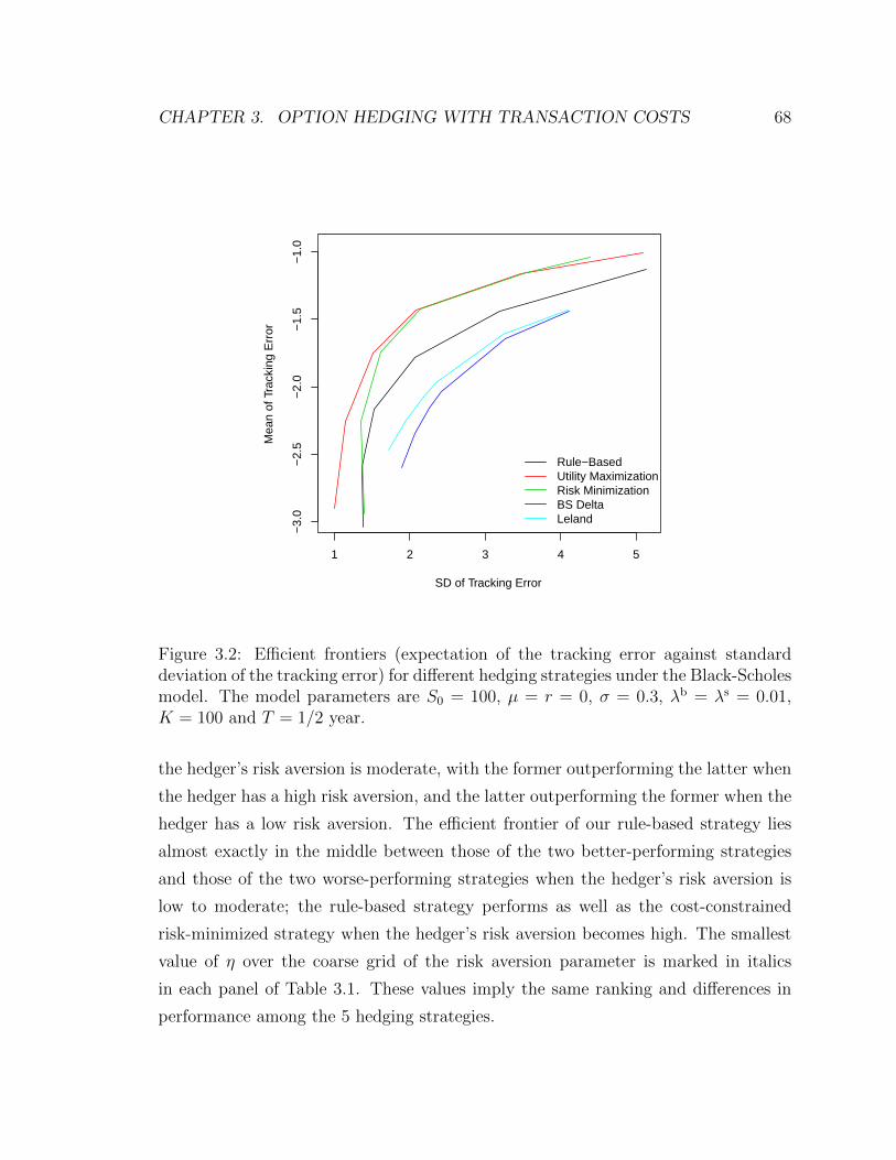
CHAPTER 3. OPTION HEDGING WITH TRANSACTION COSTS 68
1 2 3 4 5
−3.
0−
2.5
−2.
0−
1.5
−1.
0
SD of Tracking Error
Mea
n of
Tra
ckin
g E
rror
Rule−BasedUtility MaximizationRisk MinimizationBS DeltaLeland
Figure 3.2: Efficient frontiers (expectation of the tracking error against standarddeviation of the tracking error) for different hedging strategies under the Black-Scholesmodel. The model parameters are S0 = 100, µ = r = 0, σ = 0.3, λb = λs = 0.01,K = 100 and T = 1/2 year.
the hedger’s risk aversion is moderate, with the former outperforming the latter when
the hedger has a high risk aversion, and the latter outperforming the former when the
hedger has a low risk aversion. The efficient frontier of our rule-based strategy lies
almost exactly in the middle between those of the two better-performing strategies
and those of the two worse-performing strategies when the hedger’s risk aversion is
low to moderate; the rule-based strategy performs as well as the cost-constrained
risk-minimized strategy when the hedger’s risk aversion becomes high. The smallest
value of η over the coarse grid of the risk aversion parameter is marked in italics
in each panel of Table 3.1. These values imply the same ranking and differences in
performance among the 5 hedging strategies.
CHAPTER 3. OPTION HEDGING WITH TRANSACTION COSTS 69
To summarize our findings in Table 3.1 and Figure 3.2, compared to the utility-
maximized strategy and the cost-constrained risk-minimized strategy, which are known
to achieve certain optimal tradeoffs between the hedging cost and the hedging risk
under the Black-Scholes model, our rule-based strategy still gives a reasonably satis-
factory hedging performance, considering its simple form of the buy/sell boundaries
(3.15). We believe that the rule-based strategy will have more practical importance
in more realistic situations where the stock price no longer follows the Black-Scholes
model, and that it can dramatically reduce the computational complexity compared
to solving a stochastic control problem for each individual option.
3.4.2 Realized Prediction Errors
This simulation study is to mimic the real application that we will carry out in Section
3.5 for the data of S&P 500 futures options. To that end, we first generate under the
risk-neutral measure 10 two-year samples of daily stock prices from the discretized
geometric Brownian motion (3.19) for S0 = $50, r = 5%, σ = 25% and revision
interval δ = 1/252. Figure 3.3 displays these 10 two-year sample paths, generated
by using the same random numbers as in generating the sample paths of the jump
diffusion process in Figure 2.1.
Again we construct options outstanding on the stock based on the rules of the
CBOE for each stock price path. For the 10 simulated paths, the number of options
ranges from 83 to 101, with an average of 90. The buy/sell boundaries (3.15) with
(3.16) is used again and tuned to each training sample to give the smallest in-sample
realized prediction error as in the first step of the iterative two-step procedure in
Section 3.3.3. For simplicity, we assume that both r and σ are known and need not
be estimated. Panel “Training” of Table 3.2 lists the optimal value d of the boundary
parameter and the corresponding in-sample realized prediction error for each of the 10
training samples. As expected, d depends heavily on the particular training sample.
Aside from the 10 training samples, 500 test samples are independently generated
in the same manner except that the length of the test paths of daily stock prices
is six months only. For each fixed training sample, we hedge options in each test

CHAPTER 3. OPTION HEDGING WITH TRANSACTION COSTS 70
0 100 200 300 400 500
2030
4050
6070
80
Day
Sto
ck P
rice
1
2
3
4
5
6
7
8
9
10
Figure 3.3: 10 two-year sample paths (labeled 1 to 10 in corresponding colors) of dailystock prices simulated from geometric Brownian motion. The model parameters areS0 = $50, r = 5% and σ = 25%.
sample using the rule-based strategy tuned to that training sample and calculate the
out-of-sample realized prediction error ηOS. The expectation of ηOS can be estimated
by its sample mean over the 500 test samples. This averaged hedging performance
measure is then compared to the same measure given by Black-Scholes delta hedg-
ing or Leland’s strategy. For a fair comparison, the revision intervals of these two
strategies are no longer allowed to vary and are fixed to be one day. Consistent with
our findings in the previous simulation study, Leland’s strategy improves the hedging
performance over Black-Scholes delta hedging by a small reduction in the expected
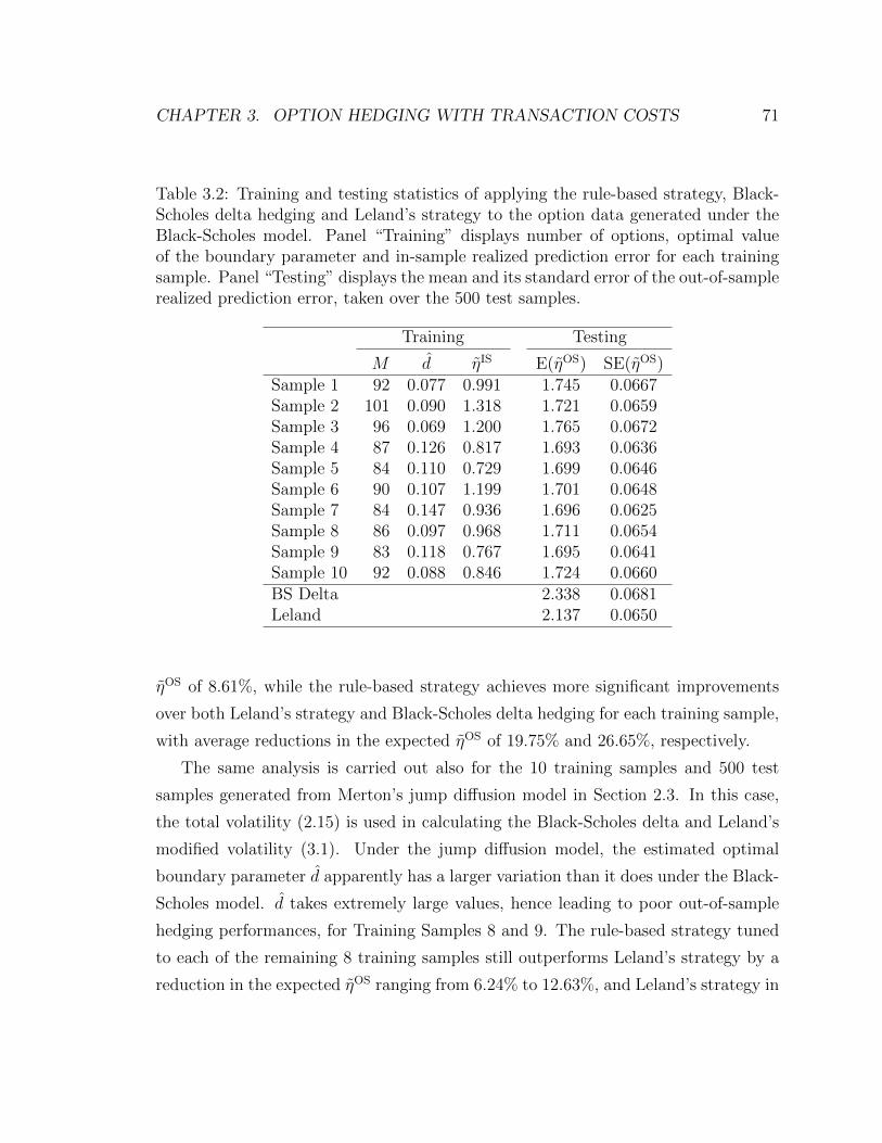
CHAPTER 3. OPTION HEDGING WITH TRANSACTION COSTS 71
Table 3.2: Training and testing statistics of applying the rule-based strategy, Black-Scholes delta hedging and Leland’s strategy to the option data generated under theBlack-Scholes model. Panel “Training” displays number of options, optimal valueof the boundary parameter and in-sample realized prediction error for each trainingsample. Panel “Testing” displays the mean and its standard error of the out-of-samplerealized prediction error, taken over the 500 test samples.
Training Testing
M d ηIS E(ηOS) SE(ηOS)Sample 1 92 0.077 0.991 1.745 0.0667Sample 2 101 0.090 1.318 1.721 0.0659Sample 3 96 0.069 1.200 1.765 0.0672Sample 4 87 0.126 0.817 1.693 0.0636Sample 5 84 0.110 0.729 1.699 0.0646Sample 6 90 0.107 1.199 1.701 0.0648Sample 7 84 0.147 0.936 1.696 0.0625Sample 8 86 0.097 0.968 1.711 0.0654Sample 9 83 0.118 0.767 1.695 0.0641Sample 10 92 0.088 0.846 1.724 0.0660BS Delta 2.338 0.0681Leland 2.137 0.0650
ηOS of 8.61%, while the rule-based strategy achieves more significant improvements
over both Leland’s strategy and Black-Scholes delta hedging for each training sample,
with average reductions in the expected ηOS of 19.75% and 26.65%, respectively.
The same analysis is carried out also for the 10 training samples and 500 test
samples generated from Merton’s jump diffusion model in Section 2.3. In this case,
the total volatility (2.15) is used in calculating the Black-Scholes delta and Leland’s
modified volatility (3.1). Under the jump diffusion model, the estimated optimal
boundary parameter d apparently has a larger variation than it does under the Black-
Scholes model. d takes extremely large values, hence leading to poor out-of-sample
hedging performances, for Training Samples 8 and 9. The rule-based strategy tuned
to each of the remaining 8 training samples still outperforms Leland’s strategy by a
reduction in the expected ηOS ranging from 6.24% to 12.63%, and Leland’s strategy in
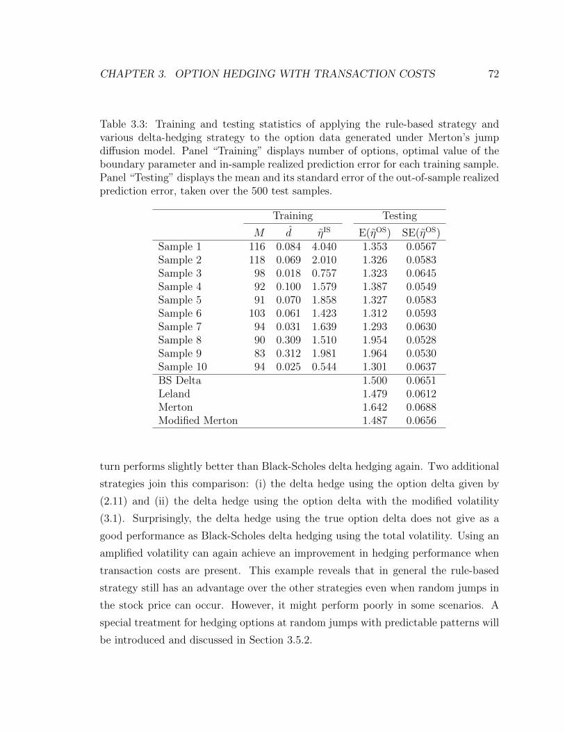
CHAPTER 3. OPTION HEDGING WITH TRANSACTION COSTS 72
Table 3.3: Training and testing statistics of applying the rule-based strategy andvarious delta-hedging strategy to the option data generated under Merton’s jumpdiffusion model. Panel “Training” displays number of options, optimal value of theboundary parameter and in-sample realized prediction error for each training sample.Panel “Testing” displays the mean and its standard error of the out-of-sample realizedprediction error, taken over the 500 test samples.
Training Testing
M d ηIS E(ηOS) SE(ηOS)Sample 1 116 0.084 4.040 1.353 0.0567Sample 2 118 0.069 2.010 1.326 0.0583Sample 3 98 0.018 0.757 1.323 0.0645Sample 4 92 0.100 1.579 1.387 0.0549Sample 5 91 0.070 1.858 1.327 0.0583Sample 6 103 0.061 1.423 1.312 0.0593Sample 7 94 0.031 1.639 1.293 0.0630Sample 8 90 0.309 1.510 1.954 0.0528Sample 9 83 0.312 1.981 1.964 0.0530Sample 10 94 0.025 0.544 1.301 0.0637BS Delta 1.500 0.0651Leland 1.479 0.0612Merton 1.642 0.0688Modified Merton 1.487 0.0656
turn performs slightly better than Black-Scholes delta hedging again. Two additional
strategies join this comparison: (i) the delta hedge using the option delta given by
(2.11) and (ii) the delta hedge using the option delta with the modified volatility
(3.1). Surprisingly, the delta hedge using the true option delta does not give as a
good performance as Black-Scholes delta hedging using the total volatility. Using an
amplified volatility can again achieve an improvement in hedging performance when
transaction costs are present. This example reveals that in general the rule-based
strategy still has an advantage over the other strategies even when random jumps in
the stock price can occur. However, it might perform poorly in some scenarios. A
special treatment for hedging options at random jumps with predictable patterns will
be introduced and discussed in Section 3.5.2.
CHAPTER 3. OPTION HEDGING WITH TRANSACTION COSTS 73
3.5 An Application to S&P 500 Futures Options
In the previous section, we have shown that our rule-based strategy can easily out-
perform the traditional Black-Scholes delta hedge and Leland’s strategy with the
modified volatility in the cases that the underlying stock prices are known to be gen-
erated from either the Black-Scholes model or Merton’s jump diffusion model. In
this section, we will apply the rule-based strategy to the data of S&P 500 futures
options that we have studied in Sections 2.4 and 2.5. The hedging performance of the
rule-based strategy will again be compared with those of Black-Scholes delta hedging
and Leland’s strategy. The rates of proportional transaction costs are assumed to be
λb = λs = 0.01. Options are assumed to be cash-settled.
3.5.1 Hedging Performance
Same as in the simulation studies, we use the buy/sell boundaries (3.15) with db(t, S) =
ds(t, S) = d in our rule-based strategy for the data of S&P 500 futures and futures
options. As described in Section 2.4.1, the data are divided into nonoverlapping six-
month subperiods. Following the procedure in Section 3.3.3, for each subperiod, we
find the optimal value of d by minimizing the realized prediction error (3.18) result-
ing from hedging the options within that subperiod. Then the buy/sell boundaries
with the optimal parameter are used to hedge options within the immediately fol-
lowing subperiod, and the thus-obtained realized prediction error is recorded as the
measure of out-of-sample hedging performance. This is repeated for each of the 43
training subperiods from December 1986 to June 2008 and their corresponding test
subperiods.
In order to obtain the buy/sell boundaries (3.15), the Black-Scholes delta (2.7)
needs to be first calculated. In the simulation studies, the two Black-Scholes model
parameters r and σ are assumed to be known. However, they are now unobservable
in reality and need to be estimated from the data. Same as in Section 2.4, we use the
yield of the 3-month Treasury bill as a surrogate for the risk-free rate r. The implied
volatility σI, defined by (2.17), is used to estimate the volatility σ. Specifically, the
volatility estimate implied from an option on the previous day is plugged into the
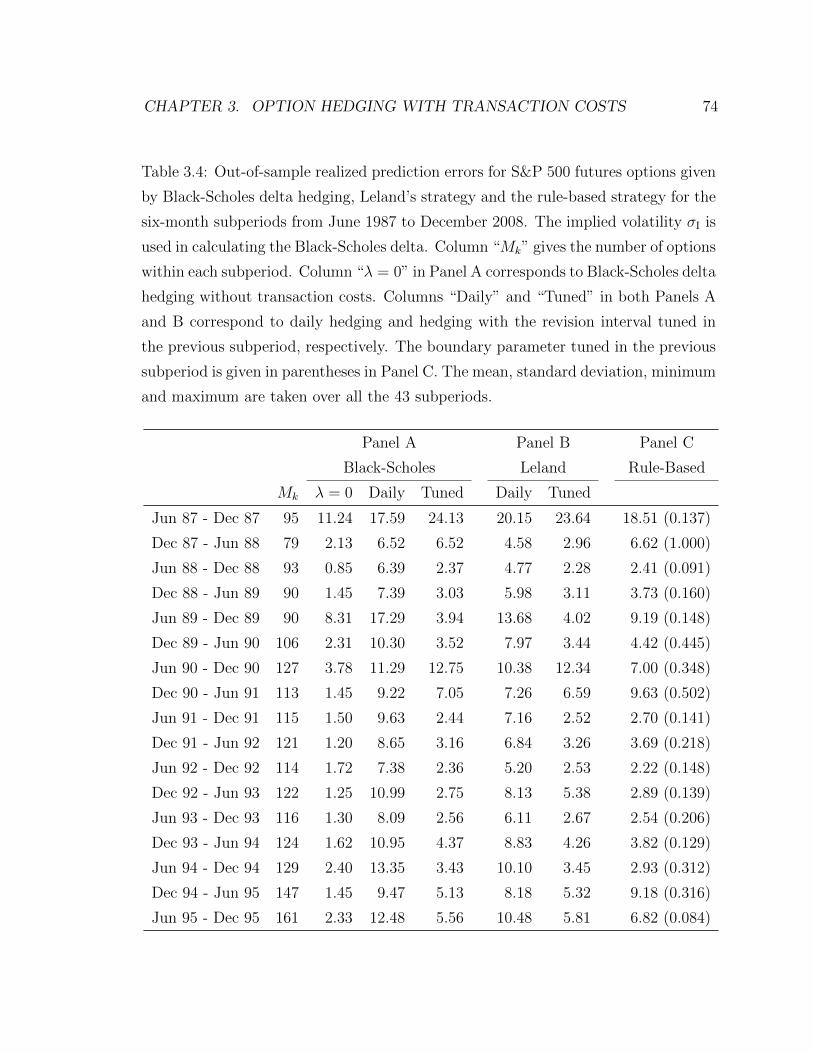
CHAPTER 3. OPTION HEDGING WITH TRANSACTION COSTS 74
Table 3.4: Out-of-sample realized prediction errors for S&P 500 futures options given
by Black-Scholes delta hedging, Leland’s strategy and the rule-based strategy for the
six-month subperiods from June 1987 to December 2008. The implied volatility σI is
used in calculating the Black-Scholes delta. Column “Mk” gives the number of options
within each subperiod. Column “λ = 0” in Panel A corresponds to Black-Scholes delta
hedging without transaction costs. Columns “Daily” and “Tuned” in both Panels A
and B correspond to daily hedging and hedging with the revision interval tuned in
the previous subperiod, respectively. The boundary parameter tuned in the previous
subperiod is given in parentheses in Panel C. The mean, standard deviation, minimum
and maximum are taken over all the 43 subperiods.
Panel A Panel B Panel C
Black-Scholes Leland Rule-Based
Mk λ = 0 Daily Tuned Daily Tuned
Jun 87 - Dec 87 95 11.24 17.59 24.13 20.15 23.64 18.51 (0.137)
Dec 87 - Jun 88 79 2.13 6.52 6.52 4.58 2.96 6.62 (1.000)
Jun 88 - Dec 88 93 0.85 6.39 2.37 4.77 2.28 2.41 (0.091)
Dec 88 - Jun 89 90 1.45 7.39 3.03 5.98 3.11 3.73 (0.160)
Jun 89 - Dec 89 90 8.31 17.29 3.94 13.68 4.02 9.19 (0.148)
Dec 89 - Jun 90 106 2.31 10.30 3.52 7.97 3.44 4.42 (0.445)
Jun 90 - Dec 90 127 3.78 11.29 12.75 10.38 12.34 7.00 (0.348)
Dec 90 - Jun 91 113 1.45 9.22 7.05 7.26 6.59 9.63 (0.502)
Jun 91 - Dec 91 115 1.50 9.63 2.44 7.16 2.52 2.70 (0.141)
Dec 91 - Jun 92 121 1.20 8.65 3.16 6.84 3.26 3.69 (0.218)
Jun 92 - Dec 92 114 1.72 7.38 2.36 5.20 2.53 2.22 (0.148)
Dec 92 - Jun 93 122 1.25 10.99 2.75 8.13 5.38 2.89 (0.139)
Jun 93 - Dec 93 116 1.30 8.09 2.56 6.11 2.67 2.54 (0.206)
Dec 93 - Jun 94 124 1.62 10.95 4.37 8.83 4.26 3.82 (0.129)
Jun 94 - Dec 94 129 2.40 13.35 3.43 10.10 3.45 2.93 (0.312)
Dec 94 - Jun 95 147 1.45 9.47 5.13 8.18 5.32 9.18 (0.316)
Jun 95 - Dec 95 161 2.33 12.48 5.56 10.48 5.81 6.82 (0.084)
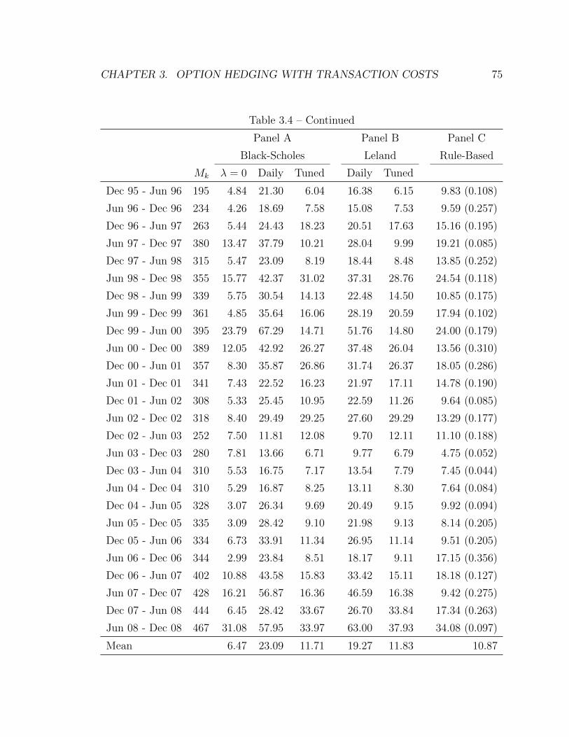
CHAPTER 3. OPTION HEDGING WITH TRANSACTION COSTS 75
Table 3.4 – Continued
Panel A Panel B Panel C
Black-Scholes Leland Rule-Based
Mk λ = 0 Daily Tuned Daily Tuned
Dec 95 - Jun 96 195 4.84 21.30 6.04 16.38 6.15 9.83 (0.108)
Jun 96 - Dec 96 234 4.26 18.69 7.58 15.08 7.53 9.59 (0.257)
Dec 96 - Jun 97 263 5.44 24.43 18.23 20.51 17.63 15.16 (0.195)
Jun 97 - Dec 97 380 13.47 37.79 10.21 28.04 9.99 19.21 (0.085)
Dec 97 - Jun 98 315 5.47 23.09 8.19 18.44 8.48 13.85 (0.252)
Jun 98 - Dec 98 355 15.77 42.37 31.02 37.31 28.76 24.54 (0.118)
Dec 98 - Jun 99 339 5.75 30.54 14.13 22.48 14.50 10.85 (0.175)
Jun 99 - Dec 99 361 4.85 35.64 16.06 28.19 20.59 17.94 (0.102)
Dec 99 - Jun 00 395 23.79 67.29 14.71 51.76 14.80 24.00 (0.179)
Jun 00 - Dec 00 389 12.05 42.92 26.27 37.48 26.04 13.56 (0.310)
Dec 00 - Jun 01 357 8.30 35.87 26.86 31.74 26.37 18.05 (0.286)
Jun 01 - Dec 01 341 7.43 22.52 16.23 21.97 17.11 14.78 (0.190)
Dec 01 - Jun 02 308 5.33 25.45 10.95 22.59 11.26 9.64 (0.085)
Jun 02 - Dec 02 318 8.40 29.49 29.25 27.60 29.29 13.29 (0.177)
Dec 02 - Jun 03 252 7.50 11.81 12.08 9.70 12.11 11.10 (0.188)
Jun 03 - Dec 03 280 7.81 13.66 6.71 9.77 6.79 4.75 (0.052)
Dec 03 - Jun 04 310 5.53 16.75 7.17 13.54 7.79 7.45 (0.044)
Jun 04 - Dec 04 310 5.29 16.87 8.25 13.11 8.30 7.64 (0.084)
Dec 04 - Jun 05 328 3.07 26.34 9.69 20.49 9.15 9.92 (0.094)
Jun 05 - Dec 05 335 3.09 28.42 9.10 21.98 9.13 8.14 (0.205)
Dec 05 - Jun 06 334 6.73 33.91 11.34 26.95 11.14 9.51 (0.205)
Jun 06 - Dec 06 344 2.99 23.84 8.51 18.17 9.11 17.15 (0.356)
Dec 06 - Jun 07 402 10.88 43.58 15.83 33.42 15.11 18.18 (0.127)
Jun 07 - Dec 07 428 16.21 56.87 16.36 46.59 16.38 9.42 (0.275)
Dec 07 - Jun 08 444 6.45 28.42 33.67 26.70 33.84 17.34 (0.263)
Jun 08 - Dec 08 467 31.08 57.95 33.97 63.00 37.93 34.08 (0.097)
Mean 6.47 23.09 11.71 19.27 11.83 10.87
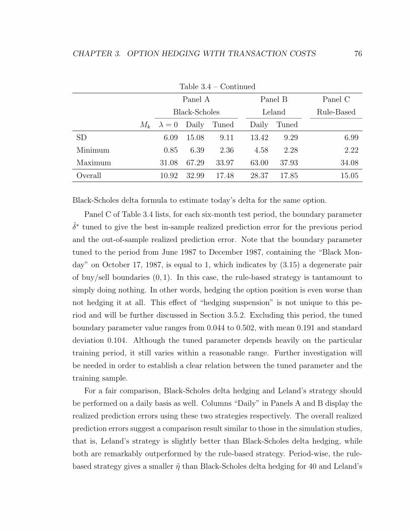
CHAPTER 3. OPTION HEDGING WITH TRANSACTION COSTS 76
Table 3.4 – Continued
Panel A Panel B Panel C
Black-Scholes Leland Rule-Based
Mk λ = 0 Daily Tuned Daily Tuned
SD 6.09 15.08 9.11 13.42 9.29 6.99
Minimum 0.85 6.39 2.36 4.58 2.28 2.22
Maximum 31.08 67.29 33.97 63.00 37.93 34.08
Overall 10.92 32.99 17.48 28.37 17.85 15.05
Black-Scholes delta formula to estimate today’s delta for the same option.
Panel C of Table 3.4 lists, for each six-month test period, the boundary parameter
δ∗ tuned to give the best in-sample realized prediction error for the previous period
and the out-of-sample realized prediction error. Note that the boundary parameter
tuned to the period from June 1987 to December 1987, containing the “Black Mon-
day” on October 17, 1987, is equal to 1, which indicates by (3.15) a degenerate pair
of buy/sell boundaries (0, 1). In this case, the rule-based strategy is tantamount to
simply doing nothing. In other words, hedging the option position is even worse than
not hedging it at all. This effect of “hedging suspension” is not unique to this pe-
riod and will be further discussed in Section 3.5.2. Excluding this period, the tuned
boundary parameter value ranges from 0.044 to 0.502, with mean 0.191 and standard
deviation 0.104. Although the tuned parameter depends heavily on the particular
training period, it still varies within a reasonable range. Further investigation will
be needed in order to establish a clear relation between the tuned parameter and the
training sample.
For a fair comparison, Black-Scholes delta hedging and Leland’s strategy should
be performed on a daily basis as well. Columns “Daily” in Panels A and B display the
realized prediction errors using these two strategies respectively. The overall realized
prediction errors suggest a comparison result similar to those in the simulation studies,
that is, Leland’s strategy is slightly better than Black-Scholes delta hedging, while
both are remarkably outperformed by the rule-based strategy. Period-wise, the rule-
based strategy gives a smaller η than Black-Scholes delta hedging for 40 and Leland’s
CHAPTER 3. OPTION HEDGING WITH TRANSACTION COSTS 77
strategy for 39 out of the 43 test periods. As a baseline, the realized prediction errors
for Black-Scholes delta hedging without transaction costs are also reported in Panel
A of Table 3.4. When transaction costs are included, although they are charged at a
rate as low as 0.01, on average, Black-Scholes delta hedging, Leland’s strategy and the
rule-based strategy incur increases of 370%, 277% and 125% respectively in realized
prediction error for each test period.
If, for Black-Scholes delta hedging and Leland’s strategy, we allow the revision
interval δ∗ to vary and regard it as a tuning parameter, their hedging performances
can be dramatically improved. Specifically, we follow an iterative procedure analogous
to the one in Section 3.3.3 for tuning the rule-based strategy:
1. The realized prediction error ηk−1 for the (k−1)-th period resulting from Black-
Scholes delta hedging or Leland’s strategy depends on δ∗, and is thus denoted
by ηk−1(δ∗). Find δ∗ = δ∗k−1 at which ηk−1(δ
∗) is minimized.
2. Hedge options within the k-th period using Black-Scholes delta hedging or
Leland’s strategy with δ∗ = δ∗k−1, and calculate the realized prediction error
ηk(δ∗k−1).
For computational simplicity, δ∗ can vary over only 1/252, 5/252, 10/252, 21/252,
42/252 and 63/252. In other words, rebalancing can only occur daily, weekly, bi-
weekly, monthly, bimonthly or trimonthly. The realized prediction errors given by
these “tuned” Black-Scholes delta hedging and Leland’s strategy are also reported in
Panels A and B of Table 3.4. The tuned Black-Scholes delta hedging (resp. tuned
Leland’s strategy) outperforms the daily Black-Scholes delta hedging (resp. daily Le-
land’s strategy) for 38 (resp. 38) out of the 43 test periods, with an average of 47.84%
(resp. 38.30%) reduction in η. However, with the tuning applied, Leland’s strategy
does not show an advantage over Black-Scholes delta hedging any more. The former
outperforms the latter for only 16 out of the 43 test periods. The rule-based strategy
gives a smaller η than the tuned Black-Scholes delta hedging (resp. tuned Leland’s
strategy) for 21 (resp. 25) test periods. Overall, it still has a slight edge over the
other two tuned strategies. However, if the revision interval is allowed to be tuned
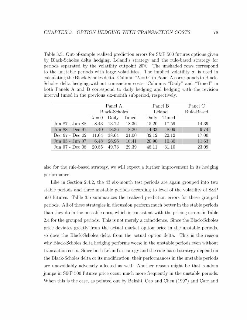
CHAPTER 3. OPTION HEDGING WITH TRANSACTION COSTS 78
Table 3.5: Out-of-sample realized prediction errors for S&P 500 futures options givenby Black-Scholes delta hedging, Leland’s strategy and the rule-based strategy forperiods separated by the volatility cutpoint 20%. The unshaded rows correspondto the unstable periods with large volatilities. The implied volatility σI is used incalculating the Black-Scholes delta. Column “λ = 0” in Panel A corresponds to Black-Scholes delta hedging without transaction costs. Columns “Daily” and “Tuned” inboth Panels A and B correspond to daily hedging and hedging with the revisioninterval tuned in the previous six-month subperiod, respectively.
Panel A Panel B Panel CBlack-Scholes Leland Rule-Based
λ = 0 Daily Tuned Daily TunedJun 87 - Jun 88 8.43 13.72 18.36 15.20 17.59 14.39Jun 88 - Dec 97 5.40 18.36 8.20 14.33 8.09 9.74Dec 97 - Dec 02 11.64 38.64 21.00 32.12 22.12 17.00Jun 03 - Jun 07 6.48 26.96 10.41 20.90 10.30 11.63Jun 07 - Dec 08 20.85 49.73 29.39 48.11 31.10 23.09
also for the rule-based strategy, we will expect a further improvement in its hedging
performance.
Like in Section 2.4.2, the 43 six-month test periods are again grouped into two
stable periods and three unstable periods according to level of the volatility of S&P
500 futures. Table 3.5 summarizes the realized prediction errors for these grouped
periods. All of these strategies in discussion perform much better in the stable periods
than they do in the unstable ones, which is consistent with the pricing errors in Table
2.4 for the grouped periods. This is not merely a coincidence. Since the Black-Scholes
price deviates greatly from the actual market option price in the unstable periods,
so does the Black-Scholes delta from the actual option delta. This is the reason
why Black-Scholes delta hedging performs worse in the unstable periods even without
transaction costs. Since both Leland’s strategy and the rule-based strategy depend on
the Black-Scholes delta or its modification, their performances in the unstable periods
are unavoidably adversely affected as well. Another reason might be that random
jumps in S&P 500 futures price occur much more frequently in the unstable periods.
When this is the case, as pointed out by Bakshi, Cao and Chen (1997) and Carr and

CHAPTER 3. OPTION HEDGING WITH TRANSACTION COSTS 79
Wu (2009), instruments other than the futures have to be used in order to hedge
out the jump risk. Despite of the poor performance of single-instrument hedging,
the rule-based strategy still gives the most stable hedging performance among all the
competing strategies in the sense that it gives the smallest η in the unstable periods.
This also can be verified by Row “SD” in the summary section of Table 3.4, in which
the rule-based strategy again gives the smallest value.
The hedging performance of each strategy is expected to vary over the expiration-
moneyness space. Therefore, we divide both dimensions into 3 regimes and examine
the hedging performance of each strategy for the options in each of the thus-obtained
9 categories. Breakpoints of 40 days and 60 days are chosen to yield short-, medium-
and long-term regimes for time to expiration, and breakpoints of 1% and −3% are
chosen to yield in-, near- and out-of-the-money regimes for log moneyness on the first
day of option trade within the six-month subperiod. These breakpoints are chosen
in such a way that the total numbers of options in any two categories over the 43
six-month periods do not differ much. Table 3.6 summarizes the realized prediction
errors for all the competing hedging strategies in discussion. This is in the same
spirit as Tables XVI and XVII of Hutchinson, Lo and Poggio (1994). Panels A and B
correspond to the two stable periods combined and the three unstable periods com-
bined, respectively. Number of options in each category is displayed in parentheses
in the corresponding row. Note that some options might be counted multiple times,
if they do not expire in six months and are traded in more than one subperiods.
We can see that the ranking of different strategies in hedging performance is almost
always consistent across the 9 categories. The rule-based strategy outperforms daily
Black-Scholes delta hedging and daily Leland’s strategy in every category. The im-
provements by the rule-based strategy over the other two, expressed as percentage
reductions in η, do not vary much across the 9 categories, either. When tuning the
hedging frequency is allowed, both Black-Scholes delta hedging and Leland’s strategy
can achieve a much better hedging performance in each category. In most categories,
the rule-based strategy gives a slightly worse performance than the tuned Black-
Scholes delta hedging and Leland’s strategy in the stable periods, while the former
outperforms the latter two by a large margin in the unstable periods. For all these
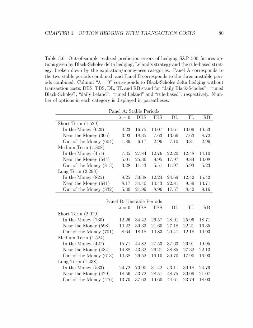
CHAPTER 3. OPTION HEDGING WITH TRANSACTION COSTS 80
Table 3.6: Out-of-sample realized prediction errors of hedging S&P 500 futures op-tions given by Black-Scholes delta hedging, Leland’s strategy and the rule-based strat-egy, broken down by the expiration/moneyness categories. Panel A corresponds tothe two stable periods combined, and Panel B corresponds to the three unstable peri-ods combined. Column “λ = 0” corresponds to Black-Scholes delta hedging withouttransaction costs; DBS, TBS, DL, TL and RB stand for “daily Black-Scholes”, “tunedBlack-Scholes”, “daily Leland”, “tuned Leland” and “rule-based”, respectively. Num-ber of options in each category is displayed in parentheses.
Panel A: Stable Periodsλ = 0 DBS TBS DL TL RB
Short Term (1,529)In the Money (620) 4.23 16.75 10.07 14.61 10.09 10.53Near the Money (305) 3.93 18.35 7.63 13.66 7.63 8.72Out of the Money (604) 1.89 6.17 2.96 7.10 3.81 2.96
Medium Term (1,808)In the Money (451) 7.35 27.84 12.76 22.20 12.48 14.10Near the Money (544) 5.01 25.36 9.95 17.97 9.84 10.08Out of the Money (813) 3.28 11.43 5.51 11.97 5.93 5.23
Long Term (2,298)In the Money (825) 9.25 30.38 12.24 24.69 12.42 15.42Near the Money (641) 8.17 34.40 10.43 22.81 9.59 13.71Out of the Money (832) 5.30 21.99 8.96 17.57 8.42 9.16
Panel B: Unstable Periodsλ = 0 DBS TBS DL TL RB
Short Term (2,029)In the Money (730) 12.26 34.42 26.57 28.91 25.96 18.71Near the Money (598) 10.22 30.33 21.60 27.18 22.21 16.35Out of the Money (701) 8.64 18.18 10.83 20.41 12.18 10.93
Medium Term (1,524)In the Money (427) 15.71 44.82 27.53 37.63 26.91 19.95Near the Money (484) 14.88 43.32 26.21 38.85 27.32 22.13Out of the Money (613) 10.38 29.52 16.10 30.70 17.90 16.93
Long Term (1,438)In the Money (533) 24.72 70.90 31.42 53.11 30.18 24.79Near the Money (429) 18.56 53.72 28.51 48.75 30.09 21.07Out of the Money (476) 13.70 37.63 19.60 44.61 23.74 18.03
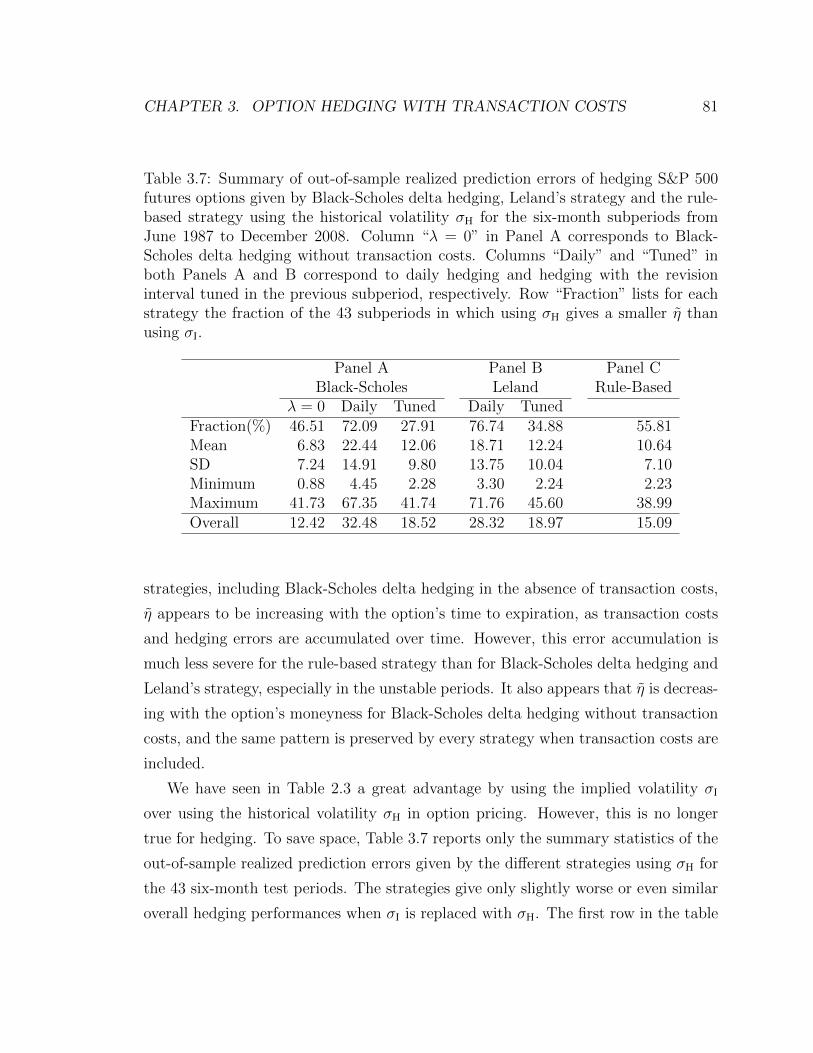
CHAPTER 3. OPTION HEDGING WITH TRANSACTION COSTS 81
Table 3.7: Summary of out-of-sample realized prediction errors of hedging S&P 500futures options given by Black-Scholes delta hedging, Leland’s strategy and the rule-based strategy using the historical volatility σH for the six-month subperiods fromJune 1987 to December 2008. Column “λ = 0” in Panel A corresponds to Black-Scholes delta hedging without transaction costs. Columns “Daily” and “Tuned” inboth Panels A and B correspond to daily hedging and hedging with the revisioninterval tuned in the previous subperiod, respectively. Row “Fraction” lists for eachstrategy the fraction of the 43 subperiods in which using σH gives a smaller η thanusing σI.
Panel A Panel B Panel CBlack-Scholes Leland Rule-Based
λ = 0 Daily Tuned Daily TunedFraction(%) 46.51 72.09 27.91 76.74 34.88 55.81Mean 6.83 22.44 12.06 18.71 12.24 10.64SD 7.24 14.91 9.80 13.75 10.04 7.10Minimum 0.88 4.45 2.28 3.30 2.24 2.23Maximum 41.73 67.35 41.74 71.76 45.60 38.99Overall 12.42 32.48 18.52 28.32 18.97 15.09
strategies, including Black-Scholes delta hedging in the absence of transaction costs,
η appears to be increasing with the option’s time to expiration, as transaction costs
and hedging errors are accumulated over time. However, this error accumulation is
much less severe for the rule-based strategy than for Black-Scholes delta hedging and
Leland’s strategy, especially in the unstable periods. It also appears that η is decreas-
ing with the option’s moneyness for Black-Scholes delta hedging without transaction
costs, and the same pattern is preserved by every strategy when transaction costs are
included.
We have seen in Table 2.3 a great advantage by using the implied volatility σI
over using the historical volatility σH in option pricing. However, this is no longer
true for hedging. To save space, Table 3.7 reports only the summary statistics of the
out-of-sample realized prediction errors given by the different strategies using σH for
the 43 six-month test periods. The strategies give only slightly worse or even similar
overall hedging performances when σI is replaced with σH. The first row in the table
CHAPTER 3. OPTION HEDGING WITH TRANSACTION COSTS 82
reports for each strategy the fraction of the 43 test periods in which using σH gives a
smaller η than using σI. We can see that, for some of the strategies, using σH gives a
better performance than using σI for a large proportion of the 43 test periods. This
suggests that a good hedging performance is much more difficult to achieve than a
good pricing performance. Both the option price and the option delta should be well
estimated in order to improve the hedging performance. However, estimating the
option delta is far from an easy task, as it is not even observable from the market.
Figures 3.4 provides another summary of the hedging performances given by the
different strategies. The histograms display the empirical distributions of the option-
wise tracking errors over the 43 six-month test periods combined from June 1987
to December 2008 given by Black-Scholes delta hedging (Panel A), Leland’s strategy
(Panel B) and the rule-based strategy (Panel C). Note that, by definition, the tracking
error VT is the option hedger’s terminal wealth. So a positive tracking error means
that the hedger actually makes a profit from hedging the option even in the presence
of transaction costs. Panel C reveals that, by following the rule-based strategy, the
hedger can make profits for a significant proportion of all the options over the whole
period, while this is not the case in Panel A for Black-Scholes delta hedging and Panel
B for Leland’s strategy, in either of which only a negligible fraction of the options end
up with a positive tracking error. Furthermore, by following the rule-based strategy,
extreme negative values of the tracking error (say, less than −$100) can be avoided,
that is, the hedger’s loss is better bounded than it is following the other two strategies.
3.5.2 Hedging Suspension at Large Jumps
Suppose that, following some strategy to hedge a short option position, one needs to
hold yt shares of stock at time t = nδ (n = 0, 1, 2, . . . , N). Consider such a scenario
that, for some 1 ≤ n < N , the stock price falls from time (n − 1)δ to time nδ and
then rises at time (n + 1)δ, that is, S(n−1)δ > Snδ < S(n+1)δ. If the hedger follows
Black-Scholes delta hedging, then we may assume that
y(n−1)δ > ynδ < y(n+1)δ, (3.20)
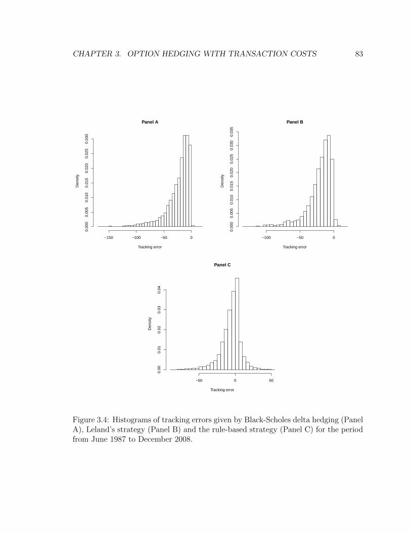
CHAPTER 3. OPTION HEDGING WITH TRANSACTION COSTS 83
Panel A
Tracking error
Den
sity
−150 −100 −50 0
0.00
00.
005
0.01
00.
015
0.02
00.
025
0.03
0
Panel B
Tracking error
Den
sity
−100 −50 0
0.00
00.
005
0.01
00.
015
0.02
00.
025
0.03
00.
035
Panel C
Tracking error
Den
sity
−50 0 50
0.00
0.01
0.02
0.03
0.04
Figure 3.4: Histograms of tracking errors given by Black-Scholes delta hedging (PanelA), Leland’s strategy (Panel B) and the rule-based strategy (Panel C) for the periodfrom June 1987 to December 2008.

CHAPTER 3. OPTION HEDGING WITH TRANSACTION COSTS 84
since the Black-Scholes delta (2.7) is an increasing function of stock price. Note
that (3.20) is not rigorously true, as the corresponding stock prices are observed at
three different time points. However, we may work around this by imposing a mild
assumption that neither S(n−1)δ/Snδ nor S(n+1)δ/Snδ is too close to 1. Since Leland’s
strategy is tantamount to Black-Scholes delta hedging with a modified volatility and
the rule-based strategy uses buy/sell boundaries (3.15) that are essentially vertical
displacements of the Black-Scholes delta, it is safe to assume that (3.20) holds for
these two strategies as well.
Under the above settings, the proceeds or loss from trading the stock over the
time period ((n− 1)δ, (n+ 1)δ] is given by
p = erδβSnδ(y(n−1)δ − ynδ)− αS(n+1)δ(y(n+1)δ − ynδ).
On the other hand, if hedging is suspended at time nδ and resumed at time (n+ 1)δ,
then the proceeds or loss from trading the stock over the same time period is instead
given by
p =
βS(n+1)δ(y(n−1)δ − y(n+1)δ) if y(n−1)δ ≥ y(n+1)δ,
αS(n+1)δ(y(n+1)δ − y(n−1)δ) if y(n−1)δ < y(n+1)δ.
We have assumed that S(n+1)δ/Snδ is not too close to 1. In particular, in the case
that it is bounded below by erδ, since β < 1 < α, we have
p < βS(n+1)δ(y(n−1)δ − ynδ)− βS(n+1)δ(y(n+1)δ − ynδ) = p
when y(n−1)δ ≥ y(n+1)δ and
p < αS(n+1)δ(y(n−1)δ − ynδ)− αS(n+1)δ(y(n+1)δ − ynδ) = p
when y(n−1)δ < y(n+1)δ. Similarly, if S(n−1)δ < Snδ > S(n+1)δ, we will also have p < p
under some mild conditions. This tells us that, if we knew that the stock price
would rise tomorrow after we saw it fall today or that it would fall tomorrow after
we saw it rise today, we would be able to raise our proceeds or reduce our loss by
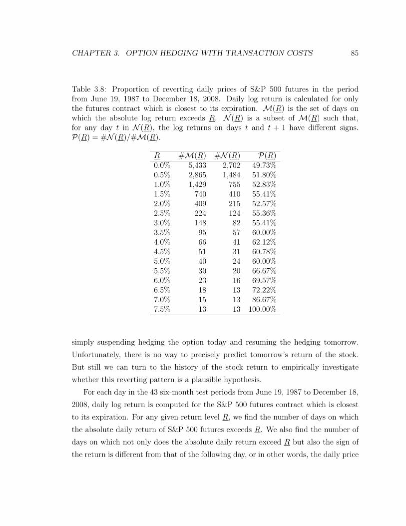
CHAPTER 3. OPTION HEDGING WITH TRANSACTION COSTS 85
Table 3.8: Proportion of reverting daily prices of S&P 500 futures in the periodfrom June 19, 1987 to December 18, 2008. Daily log return is calculated for onlythe futures contract which is closest to its expiration. M(R) is the set of days onwhich the absolute log return exceeds R. N (R) is a subset of M(R) such that,for any day t in N (R), the log returns on days t and t + 1 have different signs.P(R) = #N (R)/#M(R).
R #M(R) #N (R) P(R)0.0% 5,433 2,702 49.73%0.5% 2,865 1,484 51.80%1.0% 1,429 755 52.83%1.5% 740 410 55.41%2.0% 409 215 52.57%2.5% 224 124 55.36%3.0% 148 82 55.41%3.5% 95 57 60.00%4.0% 66 41 62.12%4.5% 51 31 60.78%5.0% 40 24 60.00%5.5% 30 20 66.67%6.0% 23 16 69.57%6.5% 18 13 72.22%7.0% 15 13 86.67%7.5% 13 13 100.00%
simply suspending hedging the option today and resuming the hedging tomorrow.
Unfortunately, there is no way to precisely predict tomorrow’s return of the stock.
But still we can turn to the history of the stock return to empirically investigate
whether this reverting pattern is a plausible hypothesis.
For each day in the 43 six-month test periods from June 19, 1987 to December 18,
2008, daily log return is computed for the S&P 500 futures contract which is closest
to its expiration. For any given return level R, we find the number of days on which
the absolute daily return of S&P 500 futures exceeds R. We also find the number of
days on which not only does the absolute daily return exceed R but also the sign of
the return is different from that of the following day, or in other words, the daily price
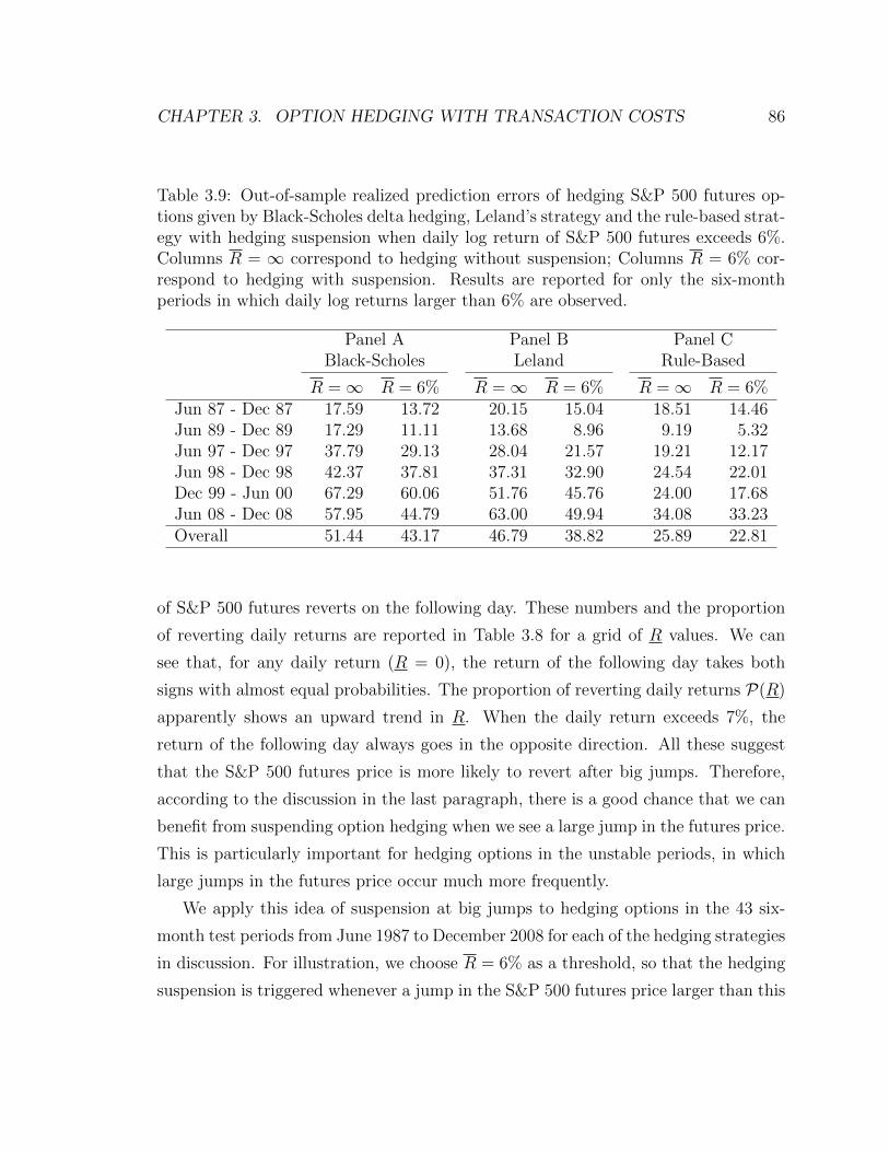
CHAPTER 3. OPTION HEDGING WITH TRANSACTION COSTS 86
Table 3.9: Out-of-sample realized prediction errors of hedging S&P 500 futures op-tions given by Black-Scholes delta hedging, Leland’s strategy and the rule-based strat-egy with hedging suspension when daily log return of S&P 500 futures exceeds 6%.Columns R = ∞ correspond to hedging without suspension; Columns R = 6% cor-respond to hedging with suspension. Results are reported for only the six-monthperiods in which daily log returns larger than 6% are observed.
Panel A Panel B Panel CBlack-Scholes Leland Rule-Based
R =∞ R = 6% R =∞ R = 6% R =∞ R = 6%Jun 87 - Dec 87 17.59 13.72 20.15 15.04 18.51 14.46Jun 89 - Dec 89 17.29 11.11 13.68 8.96 9.19 5.32Jun 97 - Dec 97 37.79 29.13 28.04 21.57 19.21 12.17Jun 98 - Dec 98 42.37 37.81 37.31 32.90 24.54 22.01Dec 99 - Jun 00 67.29 60.06 51.76 45.76 24.00 17.68Jun 08 - Dec 08 57.95 44.79 63.00 49.94 34.08 33.23Overall 51.44 43.17 46.79 38.82 25.89 22.81
of S&P 500 futures reverts on the following day. These numbers and the proportion
of reverting daily returns are reported in Table 3.8 for a grid of R values. We can
see that, for any daily return (R = 0), the return of the following day takes both
signs with almost equal probabilities. The proportion of reverting daily returns P(R)
apparently shows an upward trend in R. When the daily return exceeds 7%, the
return of the following day always goes in the opposite direction. All these suggest
that the S&P 500 futures price is more likely to revert after big jumps. Therefore,
according to the discussion in the last paragraph, there is a good chance that we can
benefit from suspending option hedging when we see a large jump in the futures price.
This is particularly important for hedging options in the unstable periods, in which
large jumps in the futures price occur much more frequently.
We apply this idea of suspension at big jumps to hedging options in the 43 six-
month test periods from June 1987 to December 2008 for each of the hedging strategies
in discussion. For illustration, we choose R = 6% as a threshold, so that the hedging
suspension is triggered whenever a jump in the S&P 500 futures price larger than this
CHAPTER 3. OPTION HEDGING WITH TRANSACTION COSTS 87
threshold occurs. Within the whole period, 23 days have seen jumps larger than 6%.
Among those days, there are 6 in the unstable period from June 1987 to December
1988 (in particular, 5 days within two weeks following the historic market crash
in October 1987), 3 in the unstable period from December 97 to December 02, an
astounding 12 in the 3-month period from September 2008 to December 2008, initially
triggered by the bankruptcy of Lehman Brothers, and 2 mini-crashes on October 13,
1989 (caused by a failed UAL deal) and October 27, 1997 (caused by an economic
crisis in Asia). Table 3.9 compares the realized prediction errors given by hedging
without suspension at large jumps and those given by hedging with suspension at
large jumps for each strategy. There are 6 six-month periods in which jumps larger
than 6% occur and hence the hedging suspension takes effect. The realized prediction
error η is reduced by the hedging suspension for each strategy and each six-month
period. The hedging suspension leads to overall percentage reductions in η of 16.06%
for Black-Scholes delta hedging, 17.02% for Leland’s strategy and 11.89% for the rule-
based strategy, respectively. The improvement in hedging performance is the least
remarkable for the rule-based strategy, as the idea of hedging suspension is already
incorporated into the use of a no-transaction region.
3.5.3 An Alternative Parameterization of the Boundaries
So far we have been using the simplest form of the buy/sell boundaries db(t, S) =
ds(t, S) = d in the rule-based strategy and achieved a great improvement in hedging
performance over the traditional Black-Scholes delta hedging and Leland’s strategy.
The question is, what if we use an alternative parameterization of the boundaries
which is more complex than the constant d. As an experiment, we assign to each of
the 9 expiration-moneyness categories in Section 3.5.1 a pair of buy/sell boundaries
of the simplest form, which is tuned to give the best hedging performance for only
the options in that category. In other words, the buy/sell boundaries have the form
(3.15) with
db(t, S) = ds(t, S) = d(j), (3.21)
CHAPTER 3. OPTION HEDGING WITH TRANSACTION COSTS 88
in which d(j) is a constant, for all the options in the j-th category C(j) (j = 1, 2, . . . , 9).
The iterative two-stage procedure in Section 3.3.3 of the rule-based strategy can be
modified as follows: for k = 1, 2, . . . and j = 1, 2, . . . , 9,
1. Use η(j)k−1(d
(j)) to denote the realized prediction error η(j)k−1 for hedging the options
in C(j) within the (k − 1)-th period using the rule-based strategy (3.15) with
(3.21). Find d(j) = d(j)k−1 that minimizes η
(j)k−1(d
(j)).
2. Hedge the options in C(j) within the k-th period using the rule-based strategy
(3.15) with db(t, S) = ds(t, S) = d(j)k−1, and calculate the realized prediction error
η(j)k (d
(j)k−1).
As an illustration, we apply this alternative parameterization of the buy/sell
boundaries to the last 13 six-month subperiods of our data of S&P 500 futures and
futures options. Excluding the first one, the 12 test subperiods cover the stable period
from June 2003 to June 2007 and the unstable period from June 2007 to December
2008. Over the 12 training subperiods, the coefficient of variation (taken over the 9
categories of options) of the tuned boundary parameter d(j)k ranges from 0.1977 to
0.6760, with an average of 0.4304, indicating a medium degree of variation across the
9 categories. Table 3.10 reports the resulting out-of-sample realized prediction errors
by the expiration-moneyness categories, compared with the same errors given by the
rule-based strategy of form (3.15) with db(t, S) = ds(t, S) = d, a global constant
independent of the categories, which has been studied in Section 3.5.1. The errors
given by the latter strategy are shown in parentheses in the table. Panel A displays
the comparison for the stable period from June 2003 to June 2007, while Panel B
displays the comparison for the unstable period from June 2007 to December 2008.
For the stable period, Strategy II (with category-wise constant d(j)) gives only a
slightly better performance than Strategy I (with global constant d) for 5 out of the 9
categories and achieves a major improvement over Strategy I for long-term out-of-the-
money options. Strategy II shows an advantage for medium- to long-term and near-
to out-of-the-money options. The overall realized prediction error given by Strategy
II for the stable period is 11.597, only slightly smaller than the error 11.625 given by
Strategy I. For the unstable period, Strategy II outperforms Strategy I for only 3 out

CHAPTER 3. OPTION HEDGING WITH TRANSACTION COSTS 89
Table 3.10: Comparison in out-of-sample realized prediction errors by the expiration-moneyness categories between the rule-based strategies with global constant d andcategory-wise constant d(j) for the period from June 2003 to December 2008. ITM,NTM and OTM stand for in-, near- and out-of-the-money, respectively. In each entry,the upper number is η given by the rule-based strategy with category-wise constantd(j), and the lower number in parentheses is η given by the rule-based strategy withglobal constant d.
Panel A: June 2003 - June 2007
ITM NTM OTM
Short Term12.300 9.832 2.055
(12.550) (9.603) (2.119)
Medium Term17.146 11.064 5.172
(16.609) (11.559) (5.477)
Long Term19.626 14.342 6.276
(18.398) (14.719) (8.080)
Panel B: June 2007 - December 2008
ITM NTM OTM
Short Term25.247 20.321 15.325
(23.739) (18.022) (16.474)
Medium Term27.873 27.437 19.250
(26.068) (27.471) (18.523)
Long Term30.404 29.617 21.045
(29.455) (27.198) (22.343)

CHAPTER 3. OPTION HEDGING WITH TRANSACTION COSTS 90
of the 9 categories, and the overall realized prediction error given by Strategy II is
23.899, slightly worse than the error 23.088 given by Strategy I.
In summary, using the more complex parameterization (3.21) for the buy/sell
boundaries in the rule-based strategy does not achieve a noticeable improvement
in hedging performance over the simplest parameterization (3.16). This coincides
with the finding that “simpler is better” by Dumas, Fleming and Whaley (1998)
for delta-hedging options using various implied volatility functions. However, we
remain conservative in our finding, as the study that we have done is far from a
thorough comparison among various parameterizations for the buy/sell boundaries.
For example, the breakpoints of the expiration-moneyness categories could also vary
and be optimally chosen according to hedging performance. Further investigation of
various forms of the boundaries will be an important topic for future research.
3.6 Conclusion
Our rule-based strategy provides a useful connection between the theoretical utility
maximization and cost-constrained risk minimization approaches and real-world ap-
plications for option hedging in the presence of proportional transaction costs. Not
only does it preserve the same feature of a no-transaction region as the theoretically
optimal strategies under the Black-Scholes model, but it is also adaptive to the de-
viation of the real data from the model via the iterative tuning for giving the best
hedging performance. Our simulation and empirical studies have demonstrated a gen-
eral advantage that the rule-based strategy possesses over Black-Scholes delta hedging
and Leland’s strategy with the modified volatility. However, all these strategies are
adversely affected by highly volatile market movements during the unstable periods,
as they all depend on the Black-Scholes delta as a starting point, which, however,
deviates greatly from the true option delta when the market is unstable. Unlike pric-
ing, option hedging with transaction costs can hardly be improved by a clever choice
of the volatility estimate. The main reason is that a good estimate for option price
does not necessarily extend to a good estimate for option delta.
It has been observed that the S&P 500 futures price is likely to revert after large

CHAPTER 3. OPTION HEDGING WITH TRANSACTION COSTS 91
jumps. Making use of this pattern, we propose to suspend rebalancing the hedging
portfolio at large jumps and resume the rebalancing in the following trading day. The
rule-based strategy, Black-Scholes delta hedging and Leland’s strategy can all benefit
from this hedging suspension for hedging S&P 500 futures options in the unstable
periods.
Using the simplest form of the buy/sell boundaries in the rule-based strategy can
already achieve a remarkable improvement in hedging performance over the other
single-instrument strategies. Our preliminary study on a more complex form of the
boundaries based on the expiration-moneyness categories of options lends support
to the use of the simplest form of the boundaries. However, we cannot reach any
conclusion until more thorough comparisons among various parameterizations of the
boundaries have been carried out. This provides us with an interesting direction for
future work.
Bibliography
Aıt-Sahalia, Y. and Lo, A. W. (1998). Nonparametric estimation of state-price
densities implicit in financial asset prices. The Journal of Finance, 53 499–547.
Almgren, R. and Chriss, N. (2000). Optimal execution of portfolio transactions.
Risk, 3 5–39.
Bakshi, G., Cao, C. and Chen, Z. (1997). Empirical performance of alternative
option pricing models. The Journal of Finance, 52 2003–2049.
Barles, G. and Soner, H. M. (1998). Option pricing with transaction costs and
a nonlinear black-scholes equation. Finance and Stochastics, 2 369–397.
Barron, A. R. (1993). Universal approximation bounds for superpositions of a
sigmoidal function. IEEE Transactions on Information Theory, 39 930–945.
Bates, D. S. (2000). Post-’87 crash fears in the S&P 500 futures option market.
Journal of Econometrics, 94 181–238.
Bensaid, B., Lesne, J.-P., Pages, H. and Scheinkman, J. (1992). Derivative
asset pricing with transaction costs. Mathematical Finance, 2 63–86.
Black, F. and Scholes, M. (1973). The pricing of options and corporate liabilities.
Journal of Political Economy, 81 637–654.
Bollerslev, T. (1986). Generalized autoregressive conditional heteroscedasticity.
Journal of Econometrics, 31 307–327.
92
BIBLIOGRAPHY 93
Boyle, P. P. and Vorst, T. (1992). Option replication in discrete time with
transaction costs. The Journal of Finance, 47 271–293.
Broadie, M., Chernov, M. and Johannes, M. (2007). Model specification and
risk premia: Evidence from futures options. The Journal of Finance, 62 1453–1490.
Broadie, M., Detemple, J., Ghysels, E. and Torres, O. (2000). Nonpara-
metric estimation of american options’ exercise boundaries and call prices. Journal
of Economic Dynamics & Control, 24 1829–1857.
Carr, P. and Wu, L. (2009). Static hedging of standard options. Working paper.
Clewlow, L. and Hodges, S. (1997). Optimal delta-hedging under transactions
costs. Journal of Economic Dynamics & Control, 21 1353–1376.
Constantinides, G. M. and Zariphopoulou, T. (1999). Bounds on prices of
contingent claims in an intertemporal economy with proportional transaction costs
and general preferences. Finance and Stochastics, 3 345–369.
Constantinides, G. M. and Zariphopoulou, T. (2001). Bounds on derivative
prices in an intertemporal setting with proportional transaction costs and multiple
securities. Mathematical Finance, 11 331–346.
Davis, M. H. A., Panas, V. G. and Zariphopoulou, T. (1993). European
option pricing with transaction costs. SIAM Journal of Control and Optimization,
31 470–493.
Derman, E. and Kani, I. (1994). Riding on the smile. Risk, 7 32–39.
Dumas, B., Fleming, J. and Whaley, R. E. (1998). Implied volatility functions:
Empirical tests. The Journal of Finance, 53 2059–2106.
Dupire, B. (1994). Pricing with a smile. Risk, 7 18–20.
Edirisifighe, C., Naik, V. and Uppal, R. (1993). Optimal replication of op-
tions with transactions costs and trading restrictions. Journal of Financial and
Quantitative Analysis, 28 117–138.
BIBLIOGRAPHY 94
Eraker, B., Johannes, M. and Polson, N. (2003). The impact of jumps in
volatility and returns. The Journal of Finance, 58 1269–1300.
Friedman, J. H. and Silverman, B. W. (1989). Flexible parsimonious smoothing
and additive modeling. Technometrics, 31 3–21.
Grinold, R. and Kahn, R. (1999). Active Portfolio Management: A Quantitative
Approach for Producing Superior Returns and Controlling Risk. 2nd ed. McGraw-
Hill, New York, NY.
Hastie, T., Tibshirani, R. and Friedman, J. (2001). The Elements of Statisti-
cal Learning: Data Mining, Inference, and Prediction. 1st ed. Springer Series in
Statistics, Springer, New York, NY.
Heston, S. (1993). A closed-form solution for options with stochastic volatility with
applications to bond and currency options. Review of Financial Studies, 6 327–343.
Hodges, S. D. and Neuberger, A. (1989). Optimal replication of contingent
claims under transaction costs. Review of Futures Markets, 8 222–239.
Hoggard, T., Whalley, A. E. and Wilmott, P. (1994). Hedging option portfo-
lios in the presence of transaction costs. Advances in Futures and Options Research,
7 21–35.
Hull, J. (2005). Options, Futures, and Other Derivatives. 6th ed. Prentice Hall,
Englewood Cliffs, NJ.
Hull, J. and White, A. (1987). The pricing of options with stochastic volatilities.
The Journal of Finance, 42 281–300.
Hutchinson, J. M., Lo, A. W. and Poggio, T. (1994). A nonparametric ap-
proach to pricing and hedging derivative securities via learning networks. The
Journal of Finance, 49 851–899.
Lai, T. L. and Lim, T. W. (2009). Option hedging theory under transaction costs.
Journal of Economic Dynamics & Control, 33 1945–1961.

BIBLIOGRAPHY 95
Lai, T. L., Liu, H. and Xing, H. (2005). Autoregressive models with piecewise
constant volatility and regression parameters. Statistica Sinica, 15 279–301.
Lai, T. L. and Wong, S. P.-S. (2004). Valuation of american options via basis
functions. IEEE Transactions on Automatic Control, 49 374–385.
Lai, T. L. and Wong, S. P.-S. (2006). Combining domain knowledge and statistical
models in time series analysis. In Time Series and Related Topics: In Memory of
Ching-Zong Wei (H.-C. Ho, C.-K. Ing and T. L. Lai, eds.), vol. 52 of Lecture Notes-
Monograph Series. Institute of Mathematical Statistics, Beachwood, OH, 193–209.
Lai, T. L. and Xing, H. (2008). Statistical Models and Methods for Financial
Markets. Springer Texts in Statistics, Springer, New York, NY.
Leland, H. E. (1985). Option pricing and replication with transactions costs. The
Journal of Finance, 40 1283–1301.
Merton, R. C. (1976). Option pricing when underlying stock returns are discon-
tinuous. Journal of Financial Economics, 3 125–144.
Merton, R. C. (1990). Continuous-Time Finance. Blackwell Publishing Ltd.,
Oxford, UK.
Navas, J. F. (2003). Calculation of volatility in a jump-diffusion model. The Journal
of Derivatives, 11 66–72.
Rubinstein, M. (1994). Implied binomial trees. The Journal of Finance, 49 771–
818.
Soner, H. M., Shreve, S. E. and Cvitanic, J. (1995). There is no nontrivial
hedging portfolio for option pricing with transaction costs. The Annals of Applied
Probability, 5 327–355.
Whalley, A. E. and Wilmott, P. (1997). An asymptotic analysis of an optimal
hedging model for option pricing with transaction costs. Mathematical Finance, 7
307–324.
BIBLIOGRAPHY 96
Zakamouline, V. (2005). Optimal hedging of options with transaction costs.
WILMOTT Magazine, July 70–82.
Zakamouline, V. (2006). European option pricing and hedging with both fixed
and proportional transaction costs. Journal of Economic Dynamics & Control, 30
1–25.
Zakamouline, V. (2008). Hedging of option portfolios and options on several assets
with transaction costs and nonlinear partial differential equations. International
Journal of Contemporary Mathematical Sciences, 3 159–180.
Zakamouline, V. (2009). The best hedging strategy in the presence of transaction
costs. International Journal of Theoretical and Applied Finance, 12 833–860.