Option Effectiveness in the Graph Model for Conflict ...

Option Effectiveness in the Graph Model

for Conflict Resolution

by

Taha Alhindi

A thesis

presented to the University of Waterloo

in fulfillment of the

thesis requirement for the degree of

Master of Applied Science

in

Systems Design Engineering

Waterloo, Ontario, Canada, 2018

©Taha Alhindi 2018

ii

AUTHOR'S DECLARATION

I hereby declare that I am the sole author of this thesis. This is a true copy of the thesis,

including any required final revisions, as accepted by my examiners.

I understand that my thesis may be made electronically available to the public.

iii

Abstract

The Graph Model for Conflict Resolution (GMCR) is expanded by designing a novel

approach for the evaluation of the effectiveness of actions or options controlled by the

decision makers (DMs) in a dispute with respect to the potential resolutions or equilibria.

This new procedure, called Option Effectiveness, determines the relative importance of each

option based on its selection within each resolution contained in the set of equilibria, as well

as the types of solution concepts, or behavior under conflict, that form the equilibria. The

solution concepts, or stability definitions, used in this method consist of Nash, Sequential

Stability (SEQ), Symmetric Metarationality (SMR), and General Metarationality (GMR).

More specifically, the strength of an equilibrium type from strongest to weakest is Nash,

SEQ, SMR, and GMR. Based on this, the effectiveness or impact of a given option is

calculated according to its presence in an equilibrium. This permits the options to be ranked

according to their importance or effectiveness in resolving the dispute under consideration.

By better understanding which options are crucial, a given DM can focus his effort on

choosing strategies which will have a bigger impact on what occurs as the conflict evolves

over time to a final resolution.

The Option Effectiveness approach was tested and refined by applying it to four different

real-world conflicts. In particular, the ongoing trade dispute between the United States (US)

and China over a number of different trade agreements and financial institutions is modeled

and analyzed at three points in time using the GMCR methodology in combination with the

iv

Option Effectiveness advancement given in this thesis. In fact, it was this particular conflict

which motivated the author to develop the Option Effectiveness approach. This trade dispute

is divided into three phases in time. The first phase starts when China leads the initiative to

establish the Asian Infrastructure Investment Bank (AIIB) and the US considers levying

countermeasures. The second phase is when the US attempts to launch the Trans Pacific

Partnership (TPP) agreement and offers China terms regarding the AIIB. In the case of China

accepting the US conditions, the US will withdraw its opposition to the AIIB and announce

a truce over it. The third phase is subsequent to the inauguration of Mr. Donald Trump as the

President of the US in early 2017 and his withdrawal of the US from the TPP while China

considers the launching of the Regional Comprehensive Economic Partnership (RCEP) trade

agreement. The Option Effectiveness approach is further illustrated by applying it to three

other conflicts: the Cuban Missile Crisis of 1962 and two environmental conflicts called the

Elmira Groundwater Contamination conflict and the Garrison Diversion Unit irrigation

dispute. The insights revealed by applying the Option Effectiveness approach to these

conflicts, confirm the advantages of utilizing the Option Effectiveness method in conflict

analysis.

v

Acknowledgements

I would like to sincerely thank my supervisors Prof. Keith W. Hipel and Prof. D. Marc

Kilgour for their continuous support and guidance towards the successful completion of my

Master of Applied Science Degree in Systems Design Engineering.

I would also like to extend my gratitude to the Custodian of the Two Holy Mosques King

Salman Bin Abdulaziz Al Saud and the Government of Kingdom of Saudi Arabia for their

generous scholarship which enabled me to pursue my Master’s degree.

I would also like to thank Prof. L. Fang and Prof. H. R. Tizhoosh for acting as readers of

my thesis and providing valuable suggestions for improving it.

Part of the content of my thesis is based upon two papers which were published in IEEE

conference proceedings and are duly references at appropriate locations within my Master’s

thesis.

Gratitude is also extended to Mr. Robert Hart who provided the services of proofreading

and editing, including correcting English errors and formatting.

vi

Dedication

I would like to dedicate my work to my parents Jaweed Alhindi and Lubna Farooqui, my

role-models, and my beloved wife Mominah Siddiqui who was there every day for me

providing me with everlasting love, comfort and support to finish my master’s degree.

vii

Table of Contents

AUTHOR'S DECLARATION ............................................................................................ ii

Abstract ................................................................................................................................ iii

Acknowledgements ............................................................................................................... v

Dedication ............................................................................................................................. vi

Table of Contents ................................................................................................................ vii

List of Figures ....................................................................................................................... x

List of Tables ........................................................................................................................ xi

List of Abbreviations ......................................................................................................... xvi

List of Symbols ................................................................................................................. xviii

Chapter 1 Introduction ........................................................................................................ 1

1.1.1 Motivation ........................................................................................................................................ 2

1.1.2 Research Objective ........................................................................................................................... 2

1.1.3 Thesis Structure ................................................................................................................................ 2

Chapter 2 Literature Review ............................................................................................... 5

2.1 Graph Model for Conflict Resolution ....................................................................................... 6

2.1.1 Fundamentals and Definitions of the Graph Model for Conflict Resolution .................................. 10

2.1.2 Solution Concepts within GMCR ................................................................................................... 12

2.2 Summary ................................................................................................................................. 15

Chapter 3 Methodology: Option Effectiveness ................................................................ 17

3.1 Strength of Equilibria .............................................................................................................. 18

3.2 Option Effectiveness ............................................................................................................... 22

3.3 Summary ................................................................................................................................. 24

viii

Chapter 4 Shifting Paradigms in the Global Political and Economic Arena ................ 26

4.1 The Emergence of the United States as a Global Superpower ................................................ 26

4.1.1 The World Bank and the International Monetary Fund .................................................................. 31

4.2 China’s Rise and Its Emergence as a World Superpower in the 21st Century ......................... 37

4.2.1 Chinese Global Economic Initiatives .............................................................................................. 41

4.3 Summary ................................................................................................................................. 43

Chapter 5 The Conflict Between China and the US over Global Trade Agreements .. 45

5.1 Conflict Background ............................................................................................................... 47

5.1.1 Implementation of AIIB prior to US Terms .................................................................................... 48

5.1.2 Introduction of TPP and US Terms for China over the AIIB ......................................................... 49

5.1.3 Post-Obama Era and Implementation of RCEP .............................................................................. 50

5.2 Methodology ........................................................................................................................... 51

5.3 Implementation of the Asian Infrastructure Investment Bank prior to United States Terms .. 53

5.3.1 Conflict Model for First Phase ........................................................................................................ 53

5.3.2 Stability Analysis of the First Phase ............................................................................................... 60

5.4 Introduction of the Trans Pacific Partnership agreement and the United States Terms for the

Asian Infrastructure Investment Bank ........................................................................................... 63

5.4.1 Model of Second Phase................................................................................................................... 64

5.4.2 Stability Analysis of the Second Phase ........................................................................................... 69

5.4.3 Hypergame Investigation of the Second Phase ............................................................................... 76

5.5 Post-Obama Era and Implementation of the Regional Comprehensive Economic Partnership

....................................................................................................................................................... 79

5.5.1 Model of Third Phase ..................................................................................................................... 80

5.5.2 Stability Analysis of the Third Phase .............................................................................................. 83

5.6 Options Effectiveness .............................................................................................................. 86

5.6.1 First Phase Option Effectiveness .................................................................................................... 86

5.6.2 Second Phase Option Effectiveness ................................................................................................ 89

ix

5.6.3 Third Phase Option Effectiveness ................................................................................................... 95

5.7 Overall Strategic Insights ........................................................................................................ 97

5.8 Summary ............................................................................................................................... 101

Chapter 6 Option Effectiveness: Case Studies ............................................................... 103

6.1 Elmira Groundwater Contamination Conflict ....................................................................... 103

6.1.1 The Conflict Model ....................................................................................................................... 104

6.1.2 Stability Analysis .......................................................................................................................... 107

6.1.3 Strength of Equilibria.................................................................................................................... 110

6.1.4 Option Effectiveness ..................................................................................................................... 111

6.2 The Cuban Missile Crisis ...................................................................................................... 113





6.3 The Garrison Diversion Unit ................................................................................................. 121





6.4 Summary ............................................................................................................................... 136

Chapter 7 Conclusions and Future Work ...................................................................... 138

7.1 Future Work .......................................................................................................................... 139

Bibliography ...................................................................................................................... 140

Appendix A: Preferential Option Effectiveness ............................................................. 154

x

List of Figures

Figure 1.1 Thesis Outline ....................................................................................................... 4

Figure 2.1 GMCR Procedure .................................................................................................. 7

Figure 3.1 Procedure for calculating the Option Effectiveness ............................................ 18

Figure 3.2 Relationships among equilibrium types .............................................................. 21

Figure 5.1 SEQ stability analysis of state 5 with respect to China ....................................... 69

Figure 5.2 SEQ stability analysis of state 5 with respect to the US ..................................... 70

Figure 5.3 Historical evolution of the conflict over the three phases ................................... 99

xi

List of Tables

Table 2.1 Basic solution concept descriptions and attributes (Fang et al., 1993) ................. 13

Table 3.1 Strength of Equilibria (Alhindi et al., 2018c), © 2018 IEEE ............................... 20

Table 3.2 Criteria for point assignment to each equilibrium state for measuring its strength

(Alhindi et al., 2018c), © 2018 IEEE ................................................................................... 22

Table 3.3 Tabular form of the Option Effectiveness approach (Alhindi et al., 2018c), ©

2018 IEEE ............................................................................................................................ 24

Table 5.1 First phase DMs’ options ..................................................................................... 54

Table 5.2 First phase option form ......................................................................................... 56

Table 5.3 First phase option prioritization for each DM ...................................................... 58

Table 5.4 First phase preference ranking of states for China ............................................... 59

Table 5.5 First phase preference ranking of states for the US .............................................. 59

Table 5.6 First phase individual stability analysis with respect to China............................. 62

Table 5.7 First phase individual stability analysis with respect to the US ........................... 62

Table 5.8 First phase stability analysis ................................................................................. 63

Table 5.9 DMs’ options (Alhindi et al., 2017b), © 2017 IEEE ............................................ 65

Table 5.10 China’s second phase option prioritization (Alhindi et al., 2017b), © 2017 IEEE

.............................................................................................................................................. 67

Table 5.11 The US’s second phase option prioritization (Alhindi et al., 2017b), © 2017

IEEE ..................................................................................................................................... 67

Table 5.12 Second phase option form (Alhindi et al., 2017b), © 2017 IEEE ...................... 72

Table 5.13 Second phase standard individual stability analysis for China .......................... 73

Table 5.14 Second phase standard individual stability analysis for the US ......................... 74

Table 5.15 Second phase standard stability analysis – Equilibria (Alhindi et al., 2017b), ©

2017 IEEE ............................................................................................................................ 75

Table 5.16 Second phase hypergame option form (Alhindi et al., 2017b), © 2017 IEEE ... 77

xii

Table 5.17 Second phase hypergame individual stability analysis for China ...................... 77

Table 5.18 Second phase hypergame individual stability analysis for the US ..................... 78

Table 5.19 Second phase hypergame stability analysis – Equilibria (Alhindi et al., 2017b),

© 2017 IEEE ........................................................................................................................ 79

Table 5.20 Third phase DMs’ options .................................................................................. 80

Table 5.21 Third phase option form ..................................................................................... 82

Table 5.22 Third phase option prioritization ........................................................................ 82

Table 5.23 Third phase preference ranking of states for China............................................ 83

Table 5.24 Third phase preference ranking of states for the US .......................................... 83

Table 5.25 Third phase individual stability analysis for China ............................................ 84

Table 5.26 Third phase individual stability analysis for the US .......................................... 85

Table 5.27 Third phase stability analysis - Equilibria .......................................................... 85

Table 5.28 Strength of Equilibria calculation for the first phase GMCR model of the

conflict between China and the US over global trade agreements ....................................... 87

Table 5.29 Tabular approach for computing the Option Effectiveness for the first phase

GMCR model of the conflict between China and the US over global trade agreements ..... 89

Table 5.30 Strength of Equilibria calculation for the second phase standard GMCR model

of the conflict between China and the US over global trade agreements (Alhindi et al.,

2018c), © 2018 IEEE ........................................................................................................... 90

Table 5.31 Tabular approach for computing the Option Effectiveness for the second phase

standard GMCR model of the conflict between China and the US over global trade

agreements (Alhindi et al., 2018c), © 2018 IEEE ................................................................ 91

Table 5.32 Strength of Equilibria calculation for the second phase hypergame GMCR

model of the conflict between China and the US over global trade agreements (Alhindi et

al., 2018c), © 2018 IEEE ..................................................................................................... 93

xiii


hypergame GMCR model of the conflict between China and the US over global trade

agreements (Alhindi et al., 2018c), © 2018 IEEE ................................................................ 94

Table 5.34 Strength of Equilibria calculation for the third phase GMCR model of the

conflict between China and the US over global trade agreements ....................................... 95

Table 5.35 Tabular approach for computing the Option Effectiveness for the third phase

GMCR model of the conflict between China and the US over global trade agreements ..... 97

Table 5.36 Evolution of the conflict over the three phases .................................................. 99

Table 6.1 Option form of the Elmira Groundwater water contamination conflict ............. 105

Table 6.2 Preference ranking of MoE in the Elmira groundwater water contamination

conflict ................................................................................................................................ 105

Table 6.3 Preference ranking of Uniroyal in the Elmira groundwater water contamination

conflict ................................................................................................................................ 106

Table 6.4 Preference ranking of Local Governments in the Elmira groundwater water

contamination conflict ........................................................................................................ 106

Table 6.5 Individual stability analysis of the Elmira groundwater water contamination

conflict with respect to MoE .............................................................................................. 107


conflict with respect to Uniroyal ........................................................................................ 108


conflict with respect to Local Governments ....................................................................... 109

Table 6.8 Stability analysis of the Elmira groundwater water contamination conflict

showing the equilibrium states ........................................................................................... 110

Table 6.9 Strength of Equilibria calculation of the Elmira groundwater water contamination

conflict model ..................................................................................................................... 111

Table 6.10 Option Effectiveness calculation of the Elmira groundwater water

contamination conflict model ............................................................................................. 112

xiv

Table 6.11 Option form of the Cuban missile crisis conflict.............................................. 115

Table 6.12 Preference ranking of the US in the Cuban missile crisis conflict ................... 116

Table 6.13 Preference ranking of the USSR in the Cuban missile crisis conflict .............. 116

Table 6.14 Individual stability analysis of the Cuban missile crisis conflict with respect to

the US ................................................................................................................................. 117

Table 6.15 Individual stability analysis of the Cuban missile crisis Conflict with respect to

the USSR ............................................................................................................................ 117

Table 6.16 Stability analysis of the Cuban missile crisis conflict showing the equilibrium

states ................................................................................................................................... 118

Table 6.17 Strength of Equilibria calculation of the Cuban missile crisis conflict model . 119

Table 6.18 Option Effectiveness calculation of the Cuban Missile Crisis conflict model . 120

Table 6.19 The possible options available for the decision makers in the Garrison Diversion

Unit conflict (Fraser & Hipel, 1984) .................................................................................. 124

Table 6.20 Option form of the Garrison Diversion Unit conflict ....................................... 125

Table 6.21 Preference ranking of US Support, US Opposition, Canadian Opposition, and

IJC in the Garrison Diversion Unit conflict ....................................................................... 126

Table 6.22 Individual stability analysis of the Garrison Diversion Unit conflict with respect

to US Support ..................................................................................................................... 128


to US Opposition ................................................................................................................ 129


to Canadian Opposition ...................................................................................................... 130


to IJC .................................................................................................................................. 131

Table 6.26 Stability analysis of the Garrison Diversion Unit conflict showing the

equilibrium states ................................................................................................................ 132

xv

Table 6.27 Strength of Equilibria calculation of the Garrison Diversion Unit conflict model

............................................................................................................................................ 133

Table 6.28 Option Effectiveness calculation of the Garrison Diversion Unit conflict model

............................................................................................................................................ 136

Table 6.29 Option importance ranking in the Garrison Diversion Unit conflict model ..... 136

Table A.1 Tabular form of Preferential Option Effectiveness approach for DM 𝑖 ............ 156

xvi

List of Abbreviations

ADB Asian Development Bank

AIIB Asian Infrastructure Investment Bank

B&R Belt and Road

Canadian Opposition Canadian Opposition to Garrison

DM Decision Maker

FCP French Communist Party

GDN Garrison Diversion Unit

GMCR Graph Model for Conflict Resolution

GMR General Metarationality

IJC International Joint Commission

IMF International Monetary Fund

Local Governments

The Regional Municipality of Waterloo and the

Township of Woolwich

MoE Ontario Ministry of Environment

NDMA N-Nitroso Dimethylamine

OBOR One Belt One Road

RCEP Regional Comprehensive Economic Partnership

SEQ Sequential Stability

xvii

SMR Symmetric Metarationality

TPP Trans Pacific Partnership

UI Unilateral Improvement

UM Unilateral Move

UN United Nations

Uniroyal Uniroyal Chemical Ltd

US United States

US Opposition United States Opposition to Garrison

US Support United States Support for Garrison

USSR Soviet Union

WTO World Trade Organization

WWI World War One

WWII World War Two

xviii

List of Symbols

⪰𝒊

Set of binary relations on 𝑺 that express DM 𝑖’s preferences

over 𝑺

𝜆 Total number of options in a conflict model

𝐴𝑖(𝑘)

Set of allowable state transitions or UMs for DM 𝑖 from 𝑘 to

another state in one step, where 𝑘 ∊ 𝑺.

𝐴𝐍\{𝒊} The set of UMs for all the DMs except 𝑖 from 𝑘, where 𝑘 ∊ 𝑺

𝐴𝑖+(𝑘) The set of UIs for DM 𝑖 from 𝑘, where 𝑘 ∊ 𝑺.

𝐴𝐍\{𝒊}+ (𝑘) The set of UIs for all the DMs except 𝑖 from 𝑘, where 𝑘 ∊ 𝑺

𝑎𝑦𝑚

A binary function which shows if the 𝑚𝑡ℎ option under 𝐸𝑦 is

selected or not. The value of the function is 1 when the option

is selected and 0 otherwise

𝑬 Set of all equilibria in a conflict model

𝐸𝑦 Equilibrium 𝑦 in 𝑬

𝐸 An equilibrium state in 𝑬

𝐸𝐹𝐹 (𝑂𝑚) Option 𝑚’s effectiveness in a conflict

𝐸𝐹𝐹𝑃𝑅𝐸𝐹𝐷𝑀𝑖 (𝑂𝑚) Option 𝑚’s preferential effectiveness with respect to DM 𝑖

𝑓

A state’s mapping function represented by 𝜆-dimensional

column vector

xix

𝐆 The graph model of a conflict

𝐺𝑖 A directed graph for DM 𝑖

𝑔1𝑠1 DM 1’s strategy associated with State 𝑠1

𝑔𝑖𝑠1 DM 𝑖’s strategy associated with State 𝑠1

𝑔𝑛𝑠1 DM 𝑛’s strategy associated with State 𝑠1

𝑖 DM in a conflict model

𝑘 State 𝑘 in 𝑺

𝑀𝑖 Total number of options available for DM 𝑖

𝑀 Total number of options available in a conflict model

𝑚 The 𝑚th option in a conflict model

N Set of DMs in a conflict model

𝑛 Total number of DMs in a conflict model

𝑂 Set of options for all DMs in a conflict model

𝑂𝑖

Set of options available in the conflict for each DM 𝑖 in a

conflict model

𝑂𝑚 The 𝑚𝑡ℎ option in 𝑂

𝑜�̅�𝑖 �̅�𝑡ℎ option for DM 𝑖

𝑂(𝐸𝑦) Set of options for equilibrium state 𝑦

𝑺𝟎 Status quo in a conflict model

xx

𝑺 Set of states or scenarios in a conflict model

𝑺𝑖𝑁𝑎𝑠ℎ The set of Nash stable states for DM 𝑖

𝑺𝑖𝑆𝐸𝑄

The set of Sequentially stable states for DM 𝑖

𝑺𝑖𝐺𝑀𝑅 The set of general metarational states for DM 𝑖

𝑺𝑖𝑆𝑀𝑅 The set of symmetric metarational states for DM 𝑖

s A state within 𝑺

𝑆𝑇𝑅(𝐸) Numerical representation of an equilibrium state’s strength

𝑆𝑇𝑅𝑃𝑅𝐸𝐹𝐷𝑀𝑖(𝐸)

Numerical representation of an equilibrium state’s preferential

strength with respect to DM 𝑖

t A state within 𝑺

𝑡𝐺𝑀𝑅(𝐸)

A binary function which shows if 𝐸 is a GMR equilibrium.

The value of the function is 1 when it is true and 0 otherwise

𝑡𝑁𝑎𝑠ℎ(𝐸)

A binary function which shows if 𝐸 is a Nash equilibrium. The

value of the function is 1 when it is true and 0 otherwise

𝑡𝑆𝐸𝑄(𝐸) A binary function which shows if 𝐸 is a SEQ equilibrium. The


𝑡𝑆𝑀𝑅(𝐸)

A binary function which shows if 𝐸 is a SMR equilibrium. The


𝑣 State 𝑣 in 𝑺

xxi

𝑦 The 𝑦th equilibrium state

𝑌 The total number of equilibria in a conflict model

1

Chapter 1

Introduction

Every day, countries and individuals participate in negotiations and conflicts. These

conflicts, for instance, can be of an economic, military, or corporate nature. Analyzing such

conflicts educates decision-makers (DMs) about a dispute, permitting them to think

strategically and thereby helping in making more calculated decisions. The Graph Model for

Conflict Resolution (GMCR) approach has been shown to be a reliable and valuable method

to analyze disputes and conflicts involving two or more DM (Fang, Hipel, & Kilgour, 1993;

Fang, Hipel, Kilgour, & Peng, 2003a, 2003b; Kilgour & Hipel, 2005, 2010; Kinsara,

Petersons, Hipel, & Kilgour, 2015b; Xu, Hipel, Kilgour, & Fang, 2018).

For example, the strategic investigation of the military and political conflict between the

United States (US) and the Soviet Union (USSR), formally known as the Cuban Missile

Crisis (Fraser & Hipel, 1982, 1984; Hipel, 2011), using GMCR methodology has shown the

GMCR approach’s capabilities in predicting the possible outcomes of a conflict. Another

illustration can be the water conflict over the Euphrates River between Syria, Iraq, and

Turkey, which demonstrates the GMCR methodology and adds the concept of the inverse

GMCR approach (Kinsara, Kilgour, & Hipel, 2015a). However, up till now, the GMCR

approach has been focused on analyzing conflicts at the level of states or scenarios. The

option effectiveness approach, a novel method presented in this thesis, allows a detailed

investigation of the conflict model at the option level, in turn allowing a DM to better

2

understand the options or the actions needed to define states, and comprehend the

consequences of selecting an option which a DM controls, thereby possibly resolving the

conflict in its favor.

1.1.1 Motivation

Analysis of the economic conflict between China and the US over global trade agreements

has shown that the conflict can be influenced to end in a more desirable resolution by adding

appropriate options (Alhindi, Hipel, & Kilgour, 2018b). Therefore, understanding the way

each option works in a conflict can add valuable insights for a DM, which would ultimately

aid him or her in choosing the best option to end the conflict at a preferred scenario.

1.1.2 Research Objective

The purpose of this thesis is to introduce a new method which allows DMs and analysts to

investigate a conflict model at the option level, rather than just investigating it at the state

level of the conflict. This novel approach is named “Option Effectiveness”, which computes

the effectiveness of each option in a conflict. It can also be useful, for instance, in classifying

the equilibria or resolutions of a conflict according to the utilization of the primary options

as suggested by Fang et al. (2003a, 2003b).

1.1.3 Thesis Structure

The thesis is divided into seven chapters. Chapter 1 discusses the GMCR approach generally

and states the motivation of the study, while the basics and fundamentals of the GMCR

methodology are reviewed in Chapter 2. Chapter 3 introduces the Option Effectiveness

3

approach as an extension to GMCR methodology, while Chapter 4 highlights the economic

politics of the US and China and the global economic aftermath of World War II. The conflict

between China and the US over global trade agreements, demonstrating the GMCR

methodology and the Option Effectiveness approach, are explained in Chapter 5. Evaluation

of the Option Effectiveness procedure is carried out in Chapter 6 by applying it to important

real-world conflict models. The conclusions of the research and future work possibilities are

discussed in Chapter 7. Figure 1.1 portrays the connections among the chapters and the

contents of the thesis.

Finally, this thesis contains some of the author’s work, both published and submitted for

publication, which includes “The Conflict Over the Asian Infrastructure Investment Bank

Involving China, USA, and Japan” (Alhindi, Hipel, & Kilgour, 2017b) © 2017 IEEE; “A

Measure for Option Effectiveness in the Graph Model for Conflict Resolution” (Alhindi,

Hipel, & Kilgour, 2018a); “The Conflict over Global Trade Agreements Between China and

the United States” (Alhindi et al., 2018b); and “Option Effectiveness in Conflict Resolution”

(Alhindi, Kilgour, &, Hipel, 2018c) © 2018 IEEE.

4

Figure 1.1 Thesis Outline

5

Chapter 2

Literature Review

Conflicts are inevitable when interests of the Decision Makers (DMs) differ. A conflict has

been defined as a situation involving two or more parties in a dispute over an issue or resource

(Fraser & Hipel, 1984). Because no extensive modeling approach mimicking real conflict,

allowing for better understanding between involved parties, and helping decision makers

(DMs) make better judgements exists, a Conflict Analysis methodology was proposed by

Fraser and Hipel (1979, 1984). A subsequent advancement in the field of conflict analysis

named Graph Model for Conflict Resolution (GMCR) was later proposed by Kilgour, Hipel,

and Fang (1987). Conflict investigation is crucial for analysts and DMs because of the

increased social and political implications of decisions (Fraser & Hipel, 1984). One needs to

fully understand the hypothetical consequences of a decision before executing it.

GMCR analyzes and predicts conflict outcomes, and can handle all conflicts, including

economic, military, or corporate (Fang et al., 1993; Kilgour & Hipel, 2005; Kilgour & Hipel,

2010; Alhindi, Hipel, & Kilgour, 2017a, 2017b; Xu et al., 2018). Typically, a conflict model,

using GMCR, specifies the DMs relevant to the conflict, the options each DM controls, and

the preference ranking for each DM (i.e., a ranking of scenarios according to DM’s

preference for how the conflict should end) ( Fang et al., 1993; Kilgour & Hipel, 2005). The

following sections explain these GMCR fundamentals.

6

2.1 Graph Model for Conflict Resolution

The GMCR methodology requires a sound understanding of the conflict. The conflict needs

to be examined as a whole rather than a series of discrete events. It consists of two main

stages: modeling and analysis (Kilgour et al., 1987; Fang et al., 1993; Kilgour & Hipel, 2005).

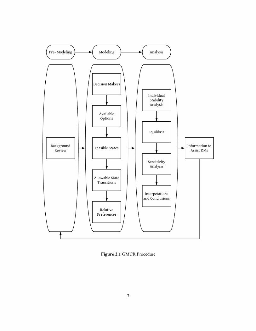
Fig 2.1 based on Hipel & Walker (2011) shows the GMCR procedure which includes the

following steps:

1) Identification of both the point in time at which the conflict is analyzed and the DMs

in the conflict.

2) Identification of the feasible scenarios, or states that may occur, in the conflict

because of option combinations available to the DMs. Options are also identified as

reversible or irreversible.

3) Elimination of any infeasible option combinations from the model, based on

conditions such as mutually exclusive options, specifying that at least one option must

be chosen within a set of options, dependency among options, or any other kind of

infeasibility that could arise (Fang et al., 2003a, 2003b). Then the allowable

transitions between feasible states are identified.

7

Figure 2.1 GMCR Procedure

8

4) Establishment of each DM’s relative preference over the feasible states. As a

consequence, unilateral improvements (UIs) and unilateral moves (UMs) can be

determined. UIs constitute allowable moves to preferred states, as compared to the

initial state; UMs constitute allowable moves from the initial state to another state,

regardless of preference.

After the fourth step of the modeling stage, the conflict model is ready for the analysis

stage. The analysis stage can be summarized as follows:

1) Individual stability analysis: This step is achieved by applying a variety of solution

concepts, including Nash stability (Nash, 1950; Nash, 1951), sequential (SEQ)

stability (Fraser & Hipel, 1979, 1984), general metarational (GMR) stability

(Howard, 1971), and symmetric metarational (SMR) stability (Howard, 1971). It

identifies the stability of each state in the model for each DM.

2) Equilibrium identification: The information gathered from the individual stability

analysis determines the equilibrium states. An equilibrium state is a state that is stable

for all DMs in the model under a given solution concept. For instance, if there are two

DMs, A and B, and if State S1 is stable for both A and B under SEQ stability then

State S1 is an equilibrium under the SEQ stability definition.

3) Sensitivity analysis: sensitivity analysis can be performed on a GMCR model by

changing, for example, the preference ranking of the states for a given DM, or by

adding or removing options.

9

4) Conclusions: The stability analysis and the sensitivity analysis help to form a strategic

understanding of the conflict, including how it may evolve and where it will resolve.

This understanding allows the DM to calculate the relative benefit of moving from

the current state.

Analyzing a conflict allows DMs to make better informed actions based on conclusions

drawn from the conflict analysis. The advantages of such analysis are listed below:

1) It permits a realistic and objective approach that analyzes complex situations based

on information retained and structured in the premodeling and modeling stages

2) It provides an easy and effective medium for communicating a conclusion about the

dispute.

3) It determines the gaps where further information is required.

4) It draws implications and conclusions from the information that was acquired during

the conflict investigation.

5) It provides clarity to the analyst or the DMs, regarding situational clarity and the

determination of a desirable course of action.

(Fraser & Hipel, 1984, p. 8)

Although the GMCR approach is simple, it is time-consuming in manual investigations of

large disputes. Software such as GMCR II (Hipel, Kilgour, Fang, & Peng, 1997; Fang et al.,

2003a, 2003b) and GMCR+ (Kinsara et al., 2015b) applies the GMCR methodology on real-

10

world conflicts and permits an easy-to-use automated approach for the understanding and

analysis of complex conflicts.

2.1.1 Fundamentals and Definitions of the Graph Model for Conflict Resolution

The GMCR methodology was first introduced by Kilgour, Hipel, and Fang (1987). The

methodology revolves around certain fundamental ideas and definitions that are explained

below. They are derived from Kilgour et al. (1987) and Kilgour & Hipel (2010).

• Decision-makers: the set of DMs is represented by N, satisfying 2 ≤ n = |N| < ∞. The

set N is usually written N = {1, 2, … , 𝑖, … , 𝑛}.

• Options: the set of options available in the conflict for each DM 𝑖 in N is represented

as 𝑂𝑖 = {𝑜�̅�𝑖 ∶ �̅� = 1, 2, … , 𝑀𝑖}, where 𝑜�̅�

𝑖 is the �̅�𝑡ℎ option for DM 𝑖 and 𝑀𝑖 is the total

number of options available for DM 𝑖.

Moreover, the set of options for all DMs in N is denoted by 𝑂 = ∪𝑖 ∈ 𝑁 𝑂𝑖.

• Strategy: The set of strategies for each DM 𝑖 is expressed by mapping function 𝑔𝑖 ∶

𝑂𝑖 → {0, 1}, where for each option �̅� = 1, 2, … , 𝑀𝑖,

𝑔𝑖(𝑜�̅�𝑖 ) = {

1, 𝑖𝑓 𝐷𝑀 𝑖 𝑠𝑒𝑙𝑒𝑐𝑡𝑠 𝑜�̅�𝑖

0, 𝑜𝑡ℎ𝑒𝑟𝑤𝑖𝑠𝑒

• States: The set of states is expressed by 𝑺 = {𝑠1, 𝑠2, … , 𝑠2𝜆}, where 2 ≤ 𝑀 = |S| <

∞, 𝑀is the total number of options available in the model and 2𝜆 is the total number of

states in the model (and will be explained later). Moreover, the status quo state is

11

represented by 𝑺𝟎. Note that a state can be represented by a mapping function 𝑓 ∶ 𝑂 →

{0, 1} such that,

𝑓(𝑜�̅�𝑖 ) = {

1, 𝑖𝑓 𝐷𝑀 𝑖 𝑠𝑒𝑙𝑒𝑐𝑡𝑠 𝑜�̅�𝑖 , 𝑓𝑜𝑟 𝑖 = 1, 2, … , 𝑛


Therefore, a state is expressed by a 𝜆-dimensional column vector, where 𝜆 is the total

number of options in 𝑂. Moreover, a state is defined by the 𝜆-dimensional column vector

in the form of (𝑓(𝑜11), 𝑓(𝑜2

1), … , 𝑓(𝑜𝑀1

1 ), … , 𝑓(𝑜1𝑛), 𝑓(𝑜2

𝑛), … , 𝑓(𝑜𝑀𝑛

𝑛 ))𝑇. The total number

of mathematically possible states in a model is 2𝜆, where 𝜆 = |𝑂|, since each option in 𝑂

can either be selected or not by the DM 𝑖 controlling it. Usually, one can eliminate some

states based on conditions such as mutual exclusivity of options, requiring that at least

one option must be selected in the scenarios, option dependency on other options, and

any other type of infeasibility that could occur (Fang et al., 2003a, 2003b). The

eliminated states constitute infeasible states, whereas the states that survived the

elimination process are feasible states. The DMs’ strategies associated with 𝑠1 are

represented as 𝑔1𝑠1 , 𝑔2

𝑠1 , … , 𝑔𝑖𝑠1 , … , 𝑔𝑛

𝑠1 ; for N = {1, 2, … , 𝑖, … , 𝑛} . Thus, states 𝑠1 is

represented by 𝑠1 = ((𝑔1𝑠1)

𝑇, (𝑔2

𝑠1)𝑇

, … , ( 𝑔𝑖𝑠1)

𝑇, … , (𝑔𝑛

𝑠1)𝑇

)𝑇

.

• Relative Preferences: For each DM 𝑖 in N, ⪰𝒊 is a complete set of binary relations on

S that express DM 𝑖’s preferences over S. Therefore, if s, t ∈ S then s ⪰𝒊 t indicates that

s is more preferred than t for DM 𝑖 or that DM 𝑖 equally prefers s to t. Following a

standard convention, DM 𝑖 firmly prefers s to t, which is mathematically expressed as s

12

≻𝑖 t, iff s ⪰𝑖 t but ¬ [t ⪰𝑖 s]. Moreover, the statement that DM 𝑖 is indifferent between s

and t, or that DM 𝑖 equally prefers s to t, is represented s ∼𝑖 t; it is valid if both s ⪰𝑖 t and

t ⪰𝑖 s.

• Transitions: For each DM 𝑖 in N, a directed graph is represented by 𝐺𝑖 = (𝑆, 𝐴𝑖)

where the arc set 𝐴𝑖 ⊆ S × S. The arc set 𝐴𝑖 does not contain loops because any entry (s,

t) ∊ 𝐴𝑖 has the property s ≠ t. Moreover, the entries or values of 𝐴𝑖(𝑘), such that 𝑘 ∊ 𝑺,

are state transitions or UMs controlled by DM 𝑖 from 𝑘. The set of UIs for DM 𝑖 from 𝑘

is denoted by 𝐴𝑖+(𝑘) where 𝑘 ∊ 𝑺.

• Graph model: the graph model of a conflict is represented by Equation 2.1.

𝐆 = ⟨𝐍, 𝐒, {𝐴𝑖: 𝑖 ∈ 𝐍}, {⪰𝑖 : 𝑖 ∈ 𝐍}⟩ (2.1)

2.1.2 Solution Concepts within GMCR

Solution concepts are a key part of the GMCR methodology, specifically for the analysis

stage. This section elaborates the attributes and properties of the solution concepts. Table 2.1

is derived from a table mentioned in “Interactive Decision Making: The Graph Model for

Conflict Resolution” published by Fang et al. (1993) and summarizes the key attributes of the

solution concepts.

2.1.2.1 Nash Stability

Nash stability revolves around the idea that a DM will always choose the alternative that

yields the most preferred possible scenario. Nash stability is formally defined in Definition

13

2.1 (Nash, 1950; Nash, 1951; Fang, Hipel, & Kilgour, 1989; Fang et al., 1993; Xu et al.,

2018). State 𝑘 is Nash stable, in a n-DM model where 𝑛 > 2, for DM 𝑖 iff 𝑖 does not have

any UIs to move to a more preferred state from 𝑘. The Nash solution concept considers only

one move in the future, requires self-knowledge of preferences, and ignores all strategic risks.

Definition 2.1 Let 𝑖 ∊ 𝐍. A state is Nash stable for DM 𝑖 , denoted by 𝑘 ∊ 𝑺𝑖𝑁𝑎𝑠ℎ , iff

𝐴𝑖+(𝑘) = ∅.

Table 2.1 Basic solution concept descriptions and attributes (Fang et al., 1993)

Solution Concepts Description

Foresight

(Future

Steps)

Knowledge

of

Preferences

Dis-

improvement

Strategic

Risk

Nash Stability

Principal DM can’t

move unilaterally to a

more preferred state

1 Own Never Ignores risk

Sequential

Stability (SEQ)

Opponents’ unilateral

improvements sanction

all concerned DM’s

unilateral improvements

2 All Never

Takes some

risks;

satisfice

Symmetric

Metarationality

(SMR)


moves sanction all

principal DM’s

unilateral improvements,

even after response by

the principal DM

3 Own By opponents’

sanctions Avoids risks

General

Metarationality

(GMR)


moves sanction all

concerned DM’s

unilateral improvements

2 Own By opponents’

sanctions Avoids risk

2.1.2.2 Sequential Stability

The SEQ stability concept is formally expressed by Definition 2.2 (Fang et al., 1993; Xu et

al., 2018). In an n-DM model where 𝑛 > 2, state 𝑘 is SEQ stable for DM 𝑖 if all the opposing

14

DMs 𝐍\{𝒊} can sanction all the UIs of 𝑖 from 𝑘 using UIs that will move 𝐍\{𝒊} to a more

preferred state 𝑣, where 𝑣 is less preferred for 𝑖 than 𝑘. SEQ stability considers two steps in

the future, requires knowledge of self and opponent’s preference rankings, and satisfices the

focal DM with respect to the outcomes.

Definition 2.2 For 𝑖 ∊ 𝐍, a state is sequentially stable (SEQ) for DM 𝑖, expressed as 𝑘 ∊

𝑺𝑖𝑆𝐸𝑄

, iff for every 𝑘1 ∊ 𝐴𝑖+(𝑘), there exists at least one 𝑘2 ∊ 𝐴𝐍\{𝒊}

+ (𝑘1 ) with 𝑘 ⪰𝑖 𝑘2.

2.1.2.3 General Metarational Stability

The GMR solution concept is formally defined in Definition 2.3 (Howard, 1971; Fang et al.,

1989; Fang et al., 1993; Xu et al., 2018) which explains that state 𝑘, in an n-DM model

where 𝑛 > 2, is GMR stable for DM 𝑖 if all the remaining DMs 𝐍\{𝒊} can sanction all the

UIs of 𝑖 from 𝑘 by UMs to another state 𝑣 which is less preferred for 𝑖 than 𝑘. GMR stability

is similar to SEQ stability; however, it does not require UIs for the DMs 𝐍\{𝒊}. GMR stability

considers two moves in the future, requires knowledge of self-preference rankings only, and

avoids all risks.

Definition 2.3 For 𝑖 ∊ 𝐍, a state is general metarational (GMR) for DM 𝑖, denoted by 𝑘 ∊

𝑺𝑖𝐺𝑀𝑅, iff for every 𝑘1 ∊ 𝐴𝑖

+(𝑘) there exists at least one 𝑘2 ∊ 𝐴𝐍\{𝒊}(𝑘1 ) with 𝑘 ⪰𝑖 𝑘2.

2.1.2.4 Symmetric Metarational Stability

The SMR solution concept is formally described in Definition 2.4 (Howard, 1971; Fang et

al., 1989; Fang et al., 1993; Xu et al., 2018). This stability definition is similar to GMR but

with an addition that allows the focal DM to consider an alternative to escape harm caused

15

by the opponents’ sanction. Thus, state 𝑘 in a n-DM model, where 𝑛 > 2, is SMR stable iff

DMs 𝐍\{𝒊} can sanction all the UIs of 𝑖 from 𝑘 using UMs to another state 𝑣, such that 𝑣 is

less preferred for 𝑖 than 𝑘, and such that there are no UIs for 𝑖 to escape from 𝑣. SMR

stability studies three moves in the future, requires knowledge of self-preference rankings,

and avoids all risks.

Definition 2.4 For 𝑖 ∊ 𝐍, a state is symmetric metarational (SMR) for DM 𝑖 denoted by

𝑘 ∊ 𝑺𝑖𝑆𝑀𝑅 , iff for every 𝑘1 ∊ 𝐴𝑖

+(𝑘) there exists at least one 𝑘2 ∊ 𝐴𝐍\{𝒊}(𝑘1 ), such that

𝑘 ⪰𝑖 𝑘2 and 𝑘 ⪰𝑖 𝑘3 for all 𝑘3 ∊ 𝐴𝑖 (𝑘2 ).

When stability has been determined for every state for all the DMs, the equilibria of the

model follow. A state is an equilibrium under a stability concept if it is stable under that

stability concept for all the DMs in the conflict. This idea can be expressed formally as in

Definition 2.5

Definition 2.5 A state 𝑘 ∊ 𝐒 is an equilibrium state under a specific solution concept, if 𝑘

is stable for all DMs in the model under the same solution concept. E is the set of all

equilibria in the conflict.

If 𝐸 ∊ E then the values of 𝑡𝑁𝑎𝑠ℎ(𝐸), 𝑡𝑆𝐸𝑄(𝐸), 𝑡𝑆𝑀𝑅(𝐸), 𝑡𝐺𝑀𝑅(𝐸) identify the type of

equilibrium. See Chapter 3 for details.

2.2 Summary

The GMCR methodology is a well-established tool for analyzing real world disputes and

predicting its possible resolutions. A conflict model within the GMCR approach constitutes

16

mainly of relative DMs in the conflict and the options they control, a set of feasible states,

and the state preference order of the DMs in the conflict. It analyzes the conflict based on

solution concepts, or behaviors under conflict, such as Nash, SEQ, SMR and GMR. The

GMCR approach enhances the DMs understanding of the conflict and allows them to take

more informed decisions in resolving conflicts.

17

Chapter 3

Methodology: Option Effectiveness

The GMCR approach has been shown to be a robust and effective method to analyze disputes

and conflicts involving two or more DMs (Fang et al., 1993; Xu et al., 2018). Previous

studies conducted by Alhindi et al. concluded that options could, in fact, be used as means to

influence the conflict and reach a more desirable resolution (Alhindi et al., 2017a, 2017b,

2018b). Therefore, knowing the effectiveness and importance of the options available at

hand for the DMs would allow a better understanding of the conflict’s direction and where it

is heading in order to resolve it. The present research proposes a novel approach to measure

options effectiveness which relies on stability analysis using GMCR (Alhindi et al., 2018a,

2018c). This approach is only usable subsequent to the stability analysis. GMCR model has

to be used first in order to conduct Nash, SEQ, GMR, and SMR Stability analyses of the

conflict, which will identify the equilibria states. Then, the strength of each equilibrium state

can be calculated. The strengths of the equilibria are then used to measure the option

effectiveness. The following subsections explain the method of calculating the strength of

an equilibrium and the option effectiveness. The procedure for Option Effectiveness is

delineated in Fig. 3.1.

This chapter includes published contents from “A Measure for Option Effectiveness in the

Graph Model for Conflict Resolution” (Alhindi et al., 2018a) and “Option Effectiveness in

Conflict Resolution” (Alhindi et al., 2018c) © 2018 IEEE.

18

Figure 3.1 Procedure for calculating the Option Effectiveness

3.1 Strength of Equilibria

For measuring the strength of the identified equilibria, a simple weighting technique is

proposed. This approach is inspired by the work of Matbouli, Kilgour, and Hipel (2015) in

measuring the robustness of an equilibrium. The strength of each equilibrium is calculated

by assigning weight points for each equilibrium state according to the solution concept that

has identified it as being an equilibrium. Certain fundamentals of GMCR are defined before

calculating the strength of the equilibria:

• Equilibrium States: Let the set of all equilibria in a conflict be represented by 𝑬 =

{𝐸1, 𝐸2, … , 𝐸𝑦, … , 𝐸𝑌}, where 𝐸𝑦 is the is the 𝑦𝑡ℎ equilibrium state and 𝑌 is the total

number of equilibrium states in a conflict.

• Equilibrium State representation in terms of the solution concepts: an equilibrium state

𝐸𝑦 is represented by the set 𝐸𝑦 = (𝑡𝑁𝑎𝑠ℎ, 𝑡𝑆𝐸𝑄 , 𝑡𝑆𝑀𝑅 , 𝑡𝐺𝑀𝑅), where:

𝑡𝑁𝑎𝑠ℎ = {1, 𝑖𝑓 𝐸𝑦 𝑖𝑠 𝑎𝑛 𝑒𝑞𝑢𝑖𝑙𝑖𝑏𝑟𝑖𝑢𝑚 𝑢𝑛𝑑𝑒𝑟 𝑁𝑎𝑠ℎ

0, 𝑜𝑡ℎ𝑒𝑟𝑤𝑖𝑠𝑒,

GMCR model stability analysis

Calculation of Strength of the Equilibria

Option Effectiveness calculation

19

𝑡𝑆𝐸𝑄 = {1, 𝑖𝑓 𝐸𝑦 𝑖𝑠 𝑎𝑛 𝑒𝑞𝑢𝑖𝑙𝑖𝑏𝑟𝑖𝑢𝑚 𝑢𝑛𝑑𝑒𝑟 𝑆𝐸𝑄


𝑡𝑆𝑀𝑅 = {1, 𝑖𝑓 𝐸𝑦 𝑖𝑠 𝑎𝑛 𝑒𝑞𝑢𝑖𝑙𝑖𝑏𝑟𝑖𝑢𝑚 𝑢𝑛𝑑𝑒𝑟 𝑆𝑀𝑅


𝑡𝐺𝑀𝑅 = {1, 𝑖𝑓 𝐸𝑦 𝑖𝑠 𝑎𝑛 𝑒𝑞𝑢𝑖𝑙𝑖𝑏𝑟𝑖𝑢𝑚 𝑢𝑛𝑑𝑒𝑟 𝐺𝑀𝑅


Once all the equilibria states are defined with respect to the stability concepts, one can

calculate the strength of an equilibrium state 𝐸 by using Equation 3.1

𝑆𝑇𝑅(𝐸𝑦) = [(𝑡𝑁𝑎𝑠ℎ × 4) + (𝑡𝑆𝐸𝑄 × 3) + (𝑡𝑆𝑀𝑅 × 2) + ( 𝑡𝐺𝑀𝑅 × 1)] (3.1)

Therefore, 𝑆𝑇𝑅(𝐸𝑦) is a numerical representation of the equilibrium strength. In this

approach, the Nash equilibrium is considered the strongest solution concept, and is given

four points since there are no UIs by which the focal DM can consider moving to a more

preferred state. The SEQ equilibrium has been ranked 2nd in terms of equilibria strength and

is assigned three points because the UIs of the focal DM can be sanctioned by UIs from the

opponent. The 3rd-ranked equilibrium is SMR, which is allotted two points, as it allows the

focal DM the chance to escape the opponent’s sanction. The weakest equilibrium states are

the ones which are GMR equilibrium and they are given one point, because the GMR stability

considers the UMs only for the focal DM and for the opponent by which he or she can

sanction the focal DM’s UMs, and unlike the SMR stability, GMR stability does not allow

the chance to escape a sanction. It can be noticed that the strength of an equilibrium state

cannot exceed 10 points. A tabular representation for calculating the equilibrium is proposed

20

which makes it easier for an analyst to perform the calculation and the comparison among

the equilibria. Table 3.1, which is named “Equilibrium Strength”, shows the proper structure

of the tabular representation of the equilibrium strength calculation in GMCR. The equilibria

of the model are listed row-wise below the “Equilibrium” heading in Table 3.1. The

equilibrium representations, in terms of the solution concepts, are listed from the 2nd to the

5th column of the table. The last column in Table 3.1 shows the strength of the equilibrium

state which is calculated by Equation 3.1. Furthermore, Table 3.2 summarizes the points

allocation criteria for the equilibrium state with respect to the solution concepts that found

the state as an equilibrium.

Table 3.1 Strength of Equilibria (Alhindi et al., 2018c), © 2018 IEEE

Equilibrium

Equilibrium representation using the solution

concepts Strength of Equilibrium

Nash (4) SEQ (3) SMR (2) GMR (1)

𝐸1 𝑡𝑁𝑎𝑠ℎ(𝐸1) 𝑡𝑆𝐸𝑄(𝐸1) 𝑡𝑆𝑀𝑅(𝐸1) 𝑡𝐺𝑀𝑅(𝐸1) 𝑆𝑇𝑅 (𝐸1)

𝐸2 𝑡𝑁𝑎𝑠ℎ(𝐸2) 𝑡𝑆𝐸𝑄(𝐸2) 𝑡𝑆𝑀𝑅(𝐸2) 𝑡𝐺𝑀𝑅(𝐸2) 𝑆𝑇𝑅 (𝐸2)

⋮ ⋮ ⋮ ⋮ ⋮ ⋮

𝐸𝑌 𝑡𝑁𝑎𝑠ℎ(𝐸𝑌) 𝑡𝑆𝐸𝑄(𝐸𝑌) 𝑡𝑆𝑀𝑅(𝐸𝑌) 𝑡𝐺𝑀𝑅(𝐸𝑌) 𝑆𝑇𝑅 (𝐸𝑌)

A state that has been identified as Nash equilibrium is also considered SEQ, SMR, and

GMR equilibrium, while a state that is SEQ equilibrium is also recognized as GMR

equilibrium and often, but not always, as SMR equilibrium. Moreover, a state that is SMR

equilibrium is always a GMR equilibrium too. Figure 3.2, which is based on a figure in an

21

article authored by Fang et al. (1989), shows a Venn diagram that illustrates the

aforementioned relationships among the equilibrium types.

Figure 3.2 Relationships among equilibrium types

22

Table 3.2 Criteria for point assignment to each equilibrium state for measuring its strength

(Alhindi et al., 2018c), © 2018 IEEE

Solution concept that

identified the state as

an equilibrium

Points

allotted Explanation

Nash 4 4 strength points are given if the state is found to be Nash

equilibrium

SEQ 3 3 strength points are assigned if the state is found to be SEQ

equilibrium

SMR 2 2 strength points are allocated if the state is found to be SMR

equilibrium

GMR 1 1 strength point is given if the state is found to be GMR

equilibrium

3.2 Option Effectiveness

The information gained by calculating the strength of the equilibria allows a general

understanding of the conflict and the possibility of an equilibrium to occur in real life.

Moreover, it is also of great importance to understand the conflict at the option level, since

the options are the basic unit on which a GMCR model is built. The Option Effectiveness

aims to provide information about the contribution of each option towards the equilibria of

the model, which would ultimately help the DMs to understand the conflict better and allow

them to rank the options in terms of their effectiveness and importance in a dispute. However,

prior to the Option Effectiveness calculation, certain fundamentals must be defined:

• Set of options in a conflict model: the set of options is {𝑂1, 𝑂2, … , 𝑂𝑚, … , 𝑂𝑀}.

• Options of an equilibrium: Equilibrium state 𝐸𝑦 can be expressed as

𝐸𝑦 = {𝑎𝑦1, 𝑎𝑦2, … , 𝑎𝑦𝑚, … , 𝑂𝑦𝑀} where

23

𝑎𝑦𝑚 = {1, 𝑖𝑓 𝑂𝑝𝑡𝑖𝑜𝑛 𝑚 𝑖𝑠 𝑠𝑒𝑙𝑒𝑐𝑡𝑒𝑑0, 𝑜𝑡ℎ𝑒𝑟𝑤𝑖𝑠𝑒

,

𝐸𝑦 is the equilibrium state, 𝑂𝑚 is the 𝑚𝑡ℎ option, which may be selected or not under

𝐸𝑦, and 𝑀 is the total number of options available.

Once the strengths of the equilibria have been calculated and the aforementioned

fundamentals established, one can calculate the effectiveness of each option. The procedure

is to sum up the strengths of the equilibrium states used to select a given option. A tabular

representation is suggested in order to ease the process of Option Effectiveness computation.

Table 3.3 is a general representation of the Option Effectiveness calculation where the

equilibrium states are listed row-wise and the options are listed column-wise. The last

column of the table shows the strength of the equilibria row-wise, calculated by Equation

3.1, and the last row shows the Option Effectiveness column-wise. In Table 3.3

The option effectiveness, denoted by 𝐸𝐹𝐹 (𝑂𝑚), can be calculated by Equation 3.2. The

values obtained using this equation are used to fill in the cells in the last row of Table 3.3 for

each option next to “Option Effectiveness”.

𝐸𝐹𝐹 (𝑂𝑚) = ∑ 𝑎𝑦𝑚

𝑌

𝑦=1

𝑆𝑇𝑅(𝐸𝑦) (3.2)

When the Option Effectiveness has been computed, one can rank the options in a model

from most important to least important in descending order, such that the options that have

higher effectiveness values are more important than the options with lower effectiveness

24

values. A tie between options in terms of effectiveness values is possible and indicates that

these options have similar importance.

Table 3.3 Tabular form of the Option Effectiveness approach (Alhindi et al., 2018c), ©

2018 IEEE

𝑂1 𝑂2 … 𝑂𝑀 Strength of

Equilibrium

𝐸1 𝑎11 𝑎12 … 𝑎1𝑀 𝑆𝑇𝑅 (𝐸1)

𝐸2 𝑎21 𝑎22 … 𝑎2𝑀 𝑆𝑇𝑅 (𝐸2)

⋮ ⋮ ⋮ ⋮ ⋮

𝐸𝑌 𝑎𝑌1 𝑎𝑌2 … 𝑎𝑌𝑀 𝑆𝑇𝑅 (𝐸𝑌)

Option Effectiveness 𝐸𝐹𝐹 (𝑂1) 𝐸𝐹𝐹 (𝑂2) … 𝐸𝐹𝐹(𝑂𝑀)

3.3 Summary

The Option Effectiveness approach is developed and designed in this thesis as an expansion

to the GMCR methodology. The procedure determines the importance or impact of each

option based on its selection within each equilibrium state in the conflict model, as well as

the types of solution concepts, or behavior under conflict, that form the equilibria. More

specifically, the strength of an equilibrium type from strongest to weakest is Nash, SEQ,

SMR, and GMR. Based on this, the effectiveness or impact of a given option is computed

according to its presence in each equilibrium state. This permits the options to be ranked

according to their importance or effectiveness in resolving the dispute under consideration.

The Option Effectiveness procedure enhances a given DM’s understanding of the impacts of

25

the options in the conflict, and in turn allowing the DM to focus his or her efforts in selecting

options that will have a larger influence in resolving the conflict.

26

Chapter 4

Shifting Paradigms in the Global Political and Economic Arena

The achievement of superpower status has been the goal of many countries around the globe

and is the underlying reason for the conflict between China and the United States (US) over

global trade agreements. The conflict is thoroughly investigated in Chapter 5. However, to

reach a sound understanding of the nature of this conflict, one needs to understand the

political history of these two nations. This chapter explains the aftermath of World War II

and the US path to global dominance, as well as the struggles of China in the mid-1900s and

its actions to improve its economy.

4.1 The Emergence of the United States as a Global Superpower

The US began to emerge as a superpower long before World War I (WWI). The main

contributing factor was the economic drive and expansion of the US. America’s geographical

presence played a vital role in its economic expansion. American soil was rich in minerals

and oil, and great for agriculture and later for industrial production. This paved the way for

international trade and commerce, which caused US ideologies, beliefs, and culture to be

transferred across the world (Mead, 2002, p. 103). Consequently, proceeds from trade were

used to strengthen US defense, particularly the navy, which was helpful in transporting its

produce internationally. Furthermore, this wealth was accompanied with advanced

technological innovation, research and development, which led to increased production and

enhanced output quality, further improving the economic capabilities of the US (Abramovitz

27

& David, 1973). As a result, rising US economic prosperity and national security enabled its

leaders to undertake crucial local and international projects that were implemented through

the use of “soft power”, resulting in US dominance in world politics (Efthymiou, 2013).

The US did not strengthen its military capacities to actively participate in world conflicts,

but rather to prevent other nations from challenging the US militarily (McDougall, 1997).

Many saw the US as being a patrolling agent that would use its military might only as a force

of good. Its leaders used mediation and soft power to further American interests and deter

conflicts amongst other nations, reinforcing its leadership and giving the US an edge in

international diplomacy (Efthymiou, 2013).

An example of the point made above can be seen in the US reluctance to participate in

WWI. It took three years for the US to join in the war, predominantly because Germany’s

naval-based warfare threatened US trade with Britain and France, and strained American

banks that had loaned substantial funds to Britain (Stevenson, 2004, p. 318; Schulzinger,

2008, p. 63). The US aim in WWI was to bring an end to the war, victory to its allies and

peace to the world, and to establish a foundation for the League of Nations to safeguard

American interests. The outcome of WWI demonstrated US supremacy, leading to its

recognition as a global superpower. Its aid to the Allies, without which victory would have

been unachievable, gave it a leading role in international affairs, particularly in European

(Stevenson, 2004, p. 319; Efthymiou, 2013).

28

With WWI coming to an end, most Americans were of the opinion that participating in

international affairs would be detrimental to America’s economy, and thus the US adopted a

policy of isolationism, a national policy that would keep the US from engaging in politically

and militarily complicated affairs. The US followed this policy throughout the 1920s up to

World War II (WWII). As a result of this policy, America’s political relations in Latin

America improved tremendously (Weisberger et al., 2018). Despite political tensions in

Europe, America persisted in its isolationist policy. In 1935, Congress passed the Neutrality

Act, which barred the supply of munitions to belligerent countries, whether they were the

target or the attacker. The same course of international policy was also maintained in the

Pacific region, where America continued to refrain from intervening in Japan’s invasion of

China in 1937. Instead, it continued to focus on peace-building and defense, strengthening

its navy and establishing security treaties with the other North and South American

governments (Weisberger et al., 2018).

However, as the world drew closer to the rise of another world-wide catastrophe after the

invasion of Poland in 1939 by Germany, known as WWII, America was compelled to revise

its neutrality act, and with the defeat of France in 1940 by Germany, it decided to supply

armaments to the Allies, specifically Britain and France, on a cash and carry basis. In fact,

the topic of the quantity of arms to be supplied to the Allies became a bone of contention

during the US election in 1940, which was won by the incumbent, Franklin Roosevelt. As

Roosevelt returned to office, he passed Lend-Lease legislation in March of 1941 which

29

further guaranteed US aid to the Allies on credit and which was also later extended to the

Soviet Union, making the US an undeclared war participant (Weisberger et al., 2018).

Moreover, the situation in the Pacific, in regard to Japan’s involvement in the war, made

US participation in the war ever more likely. Although the US had always supported China,

at the same time it was supplying Japan with commodities such as scrap metal, gas, lubricants

etc. that were crucial in Japan’s war against China. Thus, in order to support China against

Japan, the US loaned funds to China and banned the supply of scrap metal and all other types

of commodities to Japan that would prove helpful in producing munitions. From that point

in time, US relations with Japan deteriorated, as a series of events unfolded depicting Japan’s

retaliation. The biggest example of this involved Japan joining hands with Germany and

Italy and the subsequent surprise attack at Pearl Harbor which left the US with more than

three thousand casualties and confirmed the US belief that participation in the war was

unavoidable. Thus, the US formally declared war on Japan, and Germany and Italy

responded by declaring war against the US (Weisberger et al., 2018).

Although the US officially declared war when Pearl Harbor was attacked, it was not

adequately prepared for it. President Roosevelt along with his advisors had been able to

devise military plans, but due to lack of public support, sufficient expenditures had not been

allocated to the production of weaponry except for the navy, whose size was inadequate to

fight a two-ocean war. Nonetheless, the situation improved later in the war, when more than

15 million people were hired in defense services, and resources were reallocated to

30

augmenting the production of the defense industry. Consequently, an Office of War

Mobilization was founded to oversee the defense industry. The supply of raw materials was

redirected towards supporting defense production, and gradually other industries were set up

such as for synthetic rubber. Moreover, the Office of Price Administration was also

established to monitor inflation levels. Eventually, by 1944, the defense industry flourished

and arms production more than doubled the capabilities of all the opposing nations combined.

Furthermore, from the technological aspect, breakthroughs were made, and innovative

products were developed such as radar, sonar, rockets, proximity fuses, and most importantly

the atomic bomb (Weisberger et al., 2018).

Socially conditions improved as well, as unemployment declined drastically, with

employment figures reaching 53 million by 1945, leading to a shortage of manpower. The

Fair Employment Practices Committee was also founded, abolishing racial discrimination

and giving equal rights to everyone to participate in defense services, which further enhanced

production. As such, near-zero unemployment led to higher income levels, which ultimately

translated into economic prosperity for the country (Weisberger et al., 2018).

US involvement in WWII carved a new role for it in the domain of international affairs, as

it led to termination of the isolation policy and brought about the establishment of the United

Nations (UN) in 1941 by President Roosevelt and Prime Minister Winston Churchill, which

was an extension of the cooperation of the 26 Allied nations during the war. Backed with

public support for the UN, planning for the post-war structure of the UN went ahead.

https://www.britannica.com/topic/Fair-Employment-Practices-Committee

31

Eventually, on October 24th, 1945, 50 nations collaborated to lay the foundation for a

permanent United Nations, pledging the US’s commitment to a global organization with

sufficient authority to maintain an “everlasting” peace. The UN is headquartered in New

York City and is a successor to the former League of Nations, which was established during

WWI and later terminated in 1946, displaying a shift of world power from Europe to the

United States of America (Weisberger et al., 2018).

Besides the establishment of a united political charter, the UN, President Roosevelt also

encouraged economic collaboration through the creation of the two most significant

international financial bodies in the world, the World Bank and the International Monetary

Fund (IMF), at the Bretton Woods conference, the purpose of which was to eradicate the

culture of economic nationalism which placed the interests of one nation above all others

(Wan, 2016, p. 60; Weisberger et al., 2018).

The next subsection explains how the US was able to maintain its global supremacy

through utilizing the World Bank and the IMF to its political and economic advantage.

4.1.1 The World Bank and the International Monetary Fund

The World Bank is associated with the UN, and provides financial assistance to member

countries as well as developing countries by funding projects that are vital to their local

economic prosperity. It also aids developing countries with the creation of economic policies

and reorganization of their government institutions, and is responsible for setting the global

economic agenda. The IMF is also affiliated with the UN and works in collaboration with

32

the World Bank (Chossudovsky, 2018; What We Do, n.d.). According to the official IMF

website, “the primary purpose of IMF is to ensure the stability of the international monetary

system—the system of exchange rates and international payments that enables countries (and

their citizens) to transact with each other” (About the IMF, n.d., “Why the IMF was created

and how it works” para. 2). Both the World Bank and the IMF are headquartered in

Washington DC, and are together known as the Bretton Woods Institutions.

The location of the headquarters of the two largest international financial agencies in the

world expresses the magnitude of the influence the United States has on their operations.

This was one of the issues that the nations participating at the Bretton Woods conference

disagreed upon. As noted by Catherine Gwin, “the United States has viewed all multilateral

organizations, including the World Bank, as instruments of foreign policy to be used for

specific U.S. aims and objectives” (Gwin, 1997, p. 195). The US Treasury desired for the

headquarters to be located in the capital, Washington DC, which was close to the US

Congress, as opposed to the other participating nations, which favored New York City as the

better location due to its future proximity to UN headquarters. Initially, John Maynard

Keynes, a renowned British economist, proposed London as a suitable location for the

headquarters of World Bank and IMF; however, the US Secretary of the Treasury at the time,

Henry Morgenthau, was smart enough to persuade the other foreign delegations present at

the conference that locating the headquarters of the new financial institutions close to an

already established leading financial center of the world, the City of London, would cause it

33

to be dominated by the British Empire. Hence, Washington DC was looked upon as the ideal

location for the global financial institutions, situated close to the White House (Toussaint,

2014a).

Relatedly, the US Treasury also ensured that the members of the Board of Directors of the

World Bank were permanent residents in Washington DC, an idea which was greatly opposed

by Keynes, who suggested that this would cause the US government to exercise unnecessary

influence over its members. As argued by Gwin,

throughout the history of the International Bank for Reconstruction and Development

(the World bank), the United States has been the largest shareholder and the most

influential member country. U.S. support for, pressure on, and criticisms of the Bank

have been central to its growth and the evolution of its policies, programs, and

practices. (1997, p. 195)

Also, Gwin (1997) commented that “the top management of the Bank spends much more

time meeting with, consulting, and responding to the United States than it does with any other

member country. Although this intense interaction has changed little over the years” (p. 248).

Moreover, Toussaint (2014a) argued that the US government has proposed the candidate to

be elected as the president of the World Bank, which is a decision always supported by the

Board of Directors, since a representative of another member state has never been given

consideration by the Board (Toussaint, 2014a).

34

Furthermore, although reconstruction of the nations that were destroyed by WWII had been

the primary motive for why the Bank was created, nonetheless, the US government

announced the launch of the Marshall Plan (officially the European Recovery Program) to

regulate the lending operations of the World Bank (Toussaint, 2014a). In order to better

understand this notion, one must peek further into the events of 1920. At the end of WWI,

the Treaty of Versailles was signed at the Paris Peace Conference, which accused Germany

of being responsible for the War (MacMillan, 2002).

As compensation for the destruction WWI had caused, Germany became heavily indebted

to Belgium, Britain, and France, who were in turn indebted to the United States and thus

relied heavily on Germany to pay its debts so they could repay their own debts to the US.

This led to the onset of a worldwide economic recession whereby Wall Street crashed in

1929, causing Germany to default on its debts to the Allies and they to in turn default on their

US loans, leading to the Great Depression. Therefore, in order to avoid another economic

catastrophe after WWII, the US created the Marshall Plan, which was an initiative to offer

funds in the form of grants and not loans to European countries to help rebuild their

economies. This initiative would then help the US to maintain the full employment level that

was achieved during the war years due to the astronomical growth of its defense industry,

and also uphold the level of international trade. As a result, through the World Bank, the US

between 1948 and 1951 offered grants worth more than 13 billion US dollars to help

reconstruct 17 European economies, which translates to 120 billion US dollars as of today in

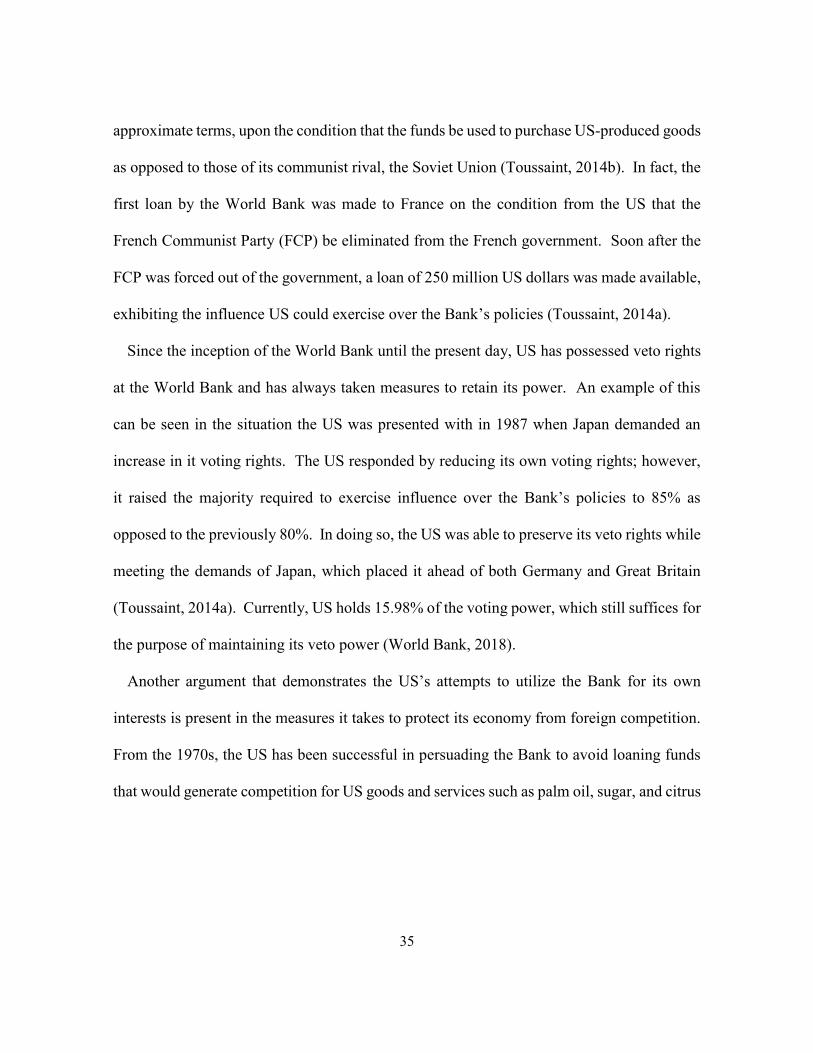
35

approximate terms, upon the condition that the funds be used to purchase US-produced goods

as opposed to those of its communist rival, the Soviet Union (Toussaint, 2014b). In fact, the

first loan by the World Bank was made to France on the condition from the US that the

French Communist Party (FCP) be eliminated from the French government. Soon after the

FCP was forced out of the government, a loan of 250 million US dollars was made available,

exhibiting the influence US could exercise over the Bank’s policies (Toussaint, 2014a).

Since the inception of the World Bank until the present day, US has possessed veto rights

at the World Bank and has always taken measures to retain its power. An example of this

can be seen in the situation the US was presented with in 1987 when Japan demanded an

increase in it voting rights. The US responded by reducing its own voting rights; however,

it raised the majority required to exercise influence over the Bank’s policies to 85% as

opposed to the previously 80%. In doing so, the US was able to preserve its veto rights while

meeting the demands of Japan, which placed it ahead of both Germany and Great Britain

(Toussaint, 2014a). Currently, US holds 15.98% of the voting power, which still suffices for

the purpose of maintaining its veto power (World Bank, 2018).

Another argument that demonstrates the US’s attempts to utilize the Bank for its own

interests is present in the measures it takes to protect its economy from foreign competition.

From the 1970s, the US has been successful in persuading the Bank to avoid loaning funds

that would generate competition for US goods and services such as palm oil, sugar, and citrus

36

fruits, and in 1987 loans to steel manufacturers in both India and Pakistan were greatly

curtailed in favor of the US economy (Toussaint, 2014a).

Conclusively, the presence of the World Bank is not only utilized as an instrument of

foreign policy by the US, but it also provides favorable financial implications for the US.

Since its inception, US contributions to the World Bank are estimated to be 1.85 billion US

dollars, whereas the Bank’s lending have amounted to 218.21 billion US dollars in total

(Toussaint, 2014a; Gwin, 1997, pp. 271-272). As further estimated by Gwin (1997), between

the period 1947 to 1992, the income of the Bank raised through the issuance of World Bank

bonds to US citizens amounted to 20.2 billion US dollars while the outlay within the US

amounted to 11 billion US dollars (pp. 271-272). This clearly demonstrates that US firms in

particular have largely benefitted from these loans (Toussaint, 2014a).

In recent years the US had been working on the Trans Pacific Partnership (TPP)

Agreement, a trade agreement to stimulate trade by reducing tariffs among participating

countries (Ablow, 2016). Negotiations regarding the TPP started under the Obama

administration, but US involvement in the TPP came to an end when President Donald Trump

withdrew the US from it in 2017 (Evans, 2017). The US withdrawal from the TPP caused a

vacuum on the global economic stage and might have paved the way for China to succeed as

the next global economic leader through China’s own international trading agreements,

which will be covered in the next section of this chapter (Wong, 2017; Sink, Olorunnipa, &

Curran, 2017).

37

For the last 100 years, the US has been able to maintain its predominance on the global

stage, backed by the influence it is capable of exerting through the World Bank and the IMF

as well as its military might. However, that predominance is being challenged by the

economic, technological, and military emergence of China, which might overshadow the

global supremacy of the US in the future.

4.2 China’s Rise and Its Emergence as a World Superpower in the 21st Century

For many centuries prior to the 18th, China was recognized as the biggest economic

superpower in the world. Hence, it can be considered that China is only re-emerging, in the

21st century, to its rightful place on the global stage. For instance, in 1078 China produced

what is estimated to be 125,000 tons of steel compared to Britain’s production, in year 1788,

of 76,000 tons. China was also leading technological innovation in the textile industry seven

centuries prior to Britain’s textile revolution in the 18th century, and China was ahead of

many nations in the trading sector with its advanced navigation systems, consisting of trade

networks reaching Europe, Africa, South Asia, and the Middle East, which helped in the

transportation of its innovative goods such as paper, weapons, book printing, and tools,

making it a manufacturing superpower. As well, China’s agricultural industry was second to

none until the 18th century. China also controlled a fleet of commercial ships considered to

be the world’s largest at the time, able to carry 3,000 tons of goods in 1588, whereas Britain’s

ships could only displace 600 tons by the end of the 18th century. The Chinese at one time

possessed around 130,000 private transport ships, and China matched Great Britain’s per

38

capita income due its robust banking industry and the high returns from the agricultural sector

(Hobson, 2004, pp. 51-73). China’s esteemed economic status was unchallenged until the

end of the 19th century (Petras, 2012).

China suffered the most from British and Western colonization of the East, which was of

a militaristic nature. These colonizing nations followed a scheme of non-equal economic

relations, and dominated opposition by military force whereas China’s prosperity was

achieved by its belief in reciprocal benefits in its trading relations (Gott, 2011). However,

failing to dominate the Chinese market by economic competition, Britain used its military

power to force its goods on China and enforcing non-reciprocal deals to lower the tariffs on

its goods. This resulted in British opium, produced in India, to overflow in China, despite

Chinese law forbidding imports of narcotics. Consequently, the Chinese suffered from the

Opium Wars with the British and millions hence being enslaved by opium. As the Chinese

rulers failed to realize the military strength of the colonizing countries, China’s esteemed

economic status met its end. As for the militaristic aspect, the British secured their

dominance over China through the enormous militarization of its economy, which was

dependent on resources apprehended from its massive colonies (Hobson, 2004). The 20th

century was devastating for China as not only had it lost its global supremacy to the West,

but most of its population was suffering from poverty and destitution. Furthermore, its main

ports were in the possession of Western countries, whereas the countryside was ruled by cruel

and immoral warlords (Petras, 2012).

39

The beginning of China's remarkable new rise can be traced back to the year 1945, when

China achieved its independence following the defeat of Japan by the US at the end of World

War II. At the time, the leadership of China was mainly divided between Mao Zedong’s

Communist Party and the Kuomintang regime of Chiang Kai-shek; this situation elevated

concerns over a new civil war (Bernstein, 2015; Kamrany & Jiang, 2015). A civil war broke

out in 1946 between the Communists and the Kuomintang, in which Mao and his communist

party emerged victorious in 1949. On October 1st, 1949 the People's Republic of China was

founded by Mao marking the beginning of the one-party government in China (BBC, n.d.;

Yu, 2015). The Communist Party’s regime worked on eradicating countryside warlords and

gangster rule, stopping the advantages of Western imperialists, and chasing down the rich

owners of blacklisted businesses such as brothels and drug- and people-trafficking. The

Chinese revolution under the Communist government was crucial in forging the current state

of China (Petras, 2012). The economic reforms were initiated by the new leaders under the

“Great Leap Forward” program aimed towards improving industrial and agricultural

productivity through mobilizing labour in order to uplift the devastated Chinese economy.

This resulted in a huge decline leading to massive casualties, and in turn, the program was

abandoned (BBC, n.d.).

The start of 1980 marked the beginning of a new era where communist China shifted its

economic policy towards a more capitalism-oriented one. In the coming decades, China

would open its market to foreign investment and privatize many state-owned industries. In

40

addition, the Chinese leadership embraced the idea of transferring technical knowledge by

providing a low-cost workforce for overseas firms. The leniency towards a capitalist

economic vision allowed China’s economy to prosper rapidly. The continued growth of

China’s manufacturing industry was a product of public investment, technological

advancement, and a firmly regulated domestic market in which both local and foreign

investment would be profiting. The Chinese government’s bold export policy and the

liberalization of the Chinese market made China one of the major exporters in the world

(Petras, 2012).

The importance of the US was evident to China, and in the 1980s, it became the main

destination for its exports (Jacques, 2012, p. 179). In 2007, China had an unprecedented

trade surplus resulting in China becoming one of the biggest creditors in the world (Hirst,

2015; Petras, 2012). In order to continue its economic dominance, China required

procurement of raw materials in huge quantities, which resulted in China investing overseas

and partnering in international trade agreements focusing on nations in Latin America and

Africa. China has maintained its policy of not interfering in the internal affairs of its trading

partners, contrary to the policy followed by its rival, the US (Petras, 2012). Furthermore,

China has started to participate in international financial organizations. For instance, it joined

the IMF and the World Bank in 1980 (Wan, 2016, p. 62) and the Asian Development Bank

(ADB) in 1986 (Wan, 2016, p. 68). However, with China being a communist country and so

viewed as suspicious by the US, delayed its participation in the World Trade Organization

41

(WTO) by almost 15 years, and after finalizing the most detailed agreements of any country,

China was able to join the WTO (Jacques, 2012, p. 178).

In the last three decades, China’s gross domestic product growth rate has averaged about

9% annually (Husna, 2018). Meanwhile, it continues to invest in energy and mineral sectors

throughout Africa. China has also been replacing US- and European-led international

financial institutions such as the IMF and the World Bank as the principle lender (Petras,

2012). As a result, Chinese influence in the last decade has grown to be tangible and real

rather than a set of statistics and speculations (Jacques, 2012, p. 409).

4.2.1 Chinese Global Economic Initiatives

In 2013, China formally initiated the idea of establishing an international bank that would

finance infrastructure projects around Asia and the world, named the Asian Infrastructure

Investment Bank, involving 57 countries in which China was the largest shareholder (About

AIIB Overview - AIIB, n.d.; Wan, 2016, pp. 44, 75). The AIIB along with China’s ever-

growing economic power is considered a direct challenge to the US and Japan, rivaling the

World Bank, the IMF, and the ADB, and increasing Chinese influence in Asia and the World

(Wan, 2016, p. 11). Some consider that the idea of establishing the AIIB was driven by the

grand Chinese plan of the Belt and Road (B&R), formally known as the One Belt One Road

(OBOR) initiative (Wan, 2016, pp. 51-52). Moreover, China’s voting share in the AIIB is

around 26%, permitting it to exercise veto rights in the bank’s decisions, as 75% of total

voting shares are needed to pass important actions (Wan, 2016, p. 50). Moreover, China’s

42

veto rights could be revoked in the case that more countries, such as the US and Japan, joined

the AIIB (Mie, 2016; Wan, 2016, p. 50). The bank’s primary focus is to finance projects

launched by the B&R (Mitrovic, 2018).

The B&R initiative, launched in 2013, involves more than 65 counties and a collective

population of 4.4 billion people. Its objective is to develop connectivity in five main areas:

people, currency, trade, infrastructure, and policy, with priority assigned to the development

of transportation networks including seaports, roads, and railways (Mitrovic, 2018).

Building infrastructure for connectivity of energy is another area of focus for the Belt and

Road initiative (Mitrovic, 2018). The initiative aims to connect Southeast Asia with Western

Europe through Chinese infrastructure, which will supposedly stimulate economic growth

across China, Asia, and the globe (Cheng, 2018; Mitrovic, 2018). The term “Belt” refers to

the Silk Road Economic Belt, similar to the ancient silk road, stretching all over Eurasia

(Cheng, 2018). The “Road” is the 21st-century Maritime Silk Road intended to connect China

to the Mediterranean Sea (Cheng, 2018). It is estimated that China is willing to invest 150

billion US dollars annually into the B&R initiative (Phillips, 2017). In fact, analysts are

indicating that this initiative has the capability to overshadow the US Marshall Plan post-

World War II (“China’s One,” 2016).

Recently, China has also been engaged in the launch of the Regional Comprehensive

Economic Partnership (RCEP) Agreement, which involves US allies such as South Korea

and Japan and is intended to be the world’s largest free-trade agreement (Brinkley, 2017).

43

The agreement focuses on free trade and lower tariffs among participating countries

(Regional Comprehensive Economic Partnership (RCEP), 2016; Regional Comprehensive

Economic Partnership, n.d.; Mathieson, 2017).

Backed by the highest foreign currency reserves in the world, valued in excess of 3.1

trillion US dollars (Picardo, 2018; IMF Data, n.d.), the AIIB, B&R, and the RCEP

agreements will enable China’s vision to emerge as the strongest economic power in the

world, surpassing the US, is clear, and its objectives to achieve that are in motion. One can

only wait and see how the future will unfold and whether the US will be able to retain its

supremacy over China.

4.3 Summary

The US has emerged as an economic and military global superpower since after WWII. It

established global financial institutions such as the IMF and the World Bank to demonstrate

its global economic influence. However, China’s unprecedented economic rise through its

economic reforms that started in the 1980s allowed it to challenge the US supremacy. It

launched its own led financial institution, the AIIB, and a unique global initiative the B&R

connecting Southeast Asia with Western Europe to increase global trade through massive

infrastructure investment. The Chinese are also working on implementing the RCEP trade

agreement to increase its economic dominance. The US withdrawal from the TPP at the start

of 2017 may have paved the way for China to act as a global economic leader. However, it

44

is yet to be seen how the future will be revealed and whether China will be able to overshadow

US dominance.

45

Chapter 5

The Conflict Between China and the US over Global Trade Agreements

In recent years, China has surprised the world with its economic and military rise. This rise

has put the United States (US) status as the world’s strongest economic superpower in

jeopardy. China is clearly in line to at least share this status with the US, if not claiming

solely for itself (Ahmed, 2011). It all started when China announced an initiative to launch

a financial institution named the Asian Infrastructure Investment Bank (AIIB) along with its

complementary initiative the Belt and Road (B&R), which would rival the US-influenced

World Bank and the Asian Development Bank (ADB), The Regional Comprehensive

Economic Partnership (RCEP) is another agreement that China is working on in parallel,

which is expected to be the world’s largest free trade agreement (Brinkley, 2017). It involves

16 countries including China and Japan (Regional Comprehensive Economic Partnership,

n.d.). Interesting facts about China’s continued rise include China becoming the world’s

second-largest economy in 2010 just behind the US, and China becoming the biggest US

creditor in recent years. As for the military aspect, China’s military spending reached more

than 45 billion dollars in 2007 (“Timeline: U.S. Relations,” n.d.). However, the US had plans

of its own such as the Trans Pacific Partnership (TPP) Agreement, a trade agreement focusing

on increasing trade by lowering tariffs among participating countries. Negotiations regarding

the TPP started under the Obama administration, but US involvement in the TPP came to an

end when President Donald Trump withdrew the US from it in 2017. The trade war between

46

China and the US was ignited when the Trump administration put forward an act to enforce

tariffs, estimated to be in the region of 60 billion US dollars, on Chinese imports (Breuninger

& Tausche, 2018), whereas China countered the act by threatening to impose tariffs on US

imports (Thomas & Wiseman, 2018).

The trade dispute between China and the US is of great importance, and a thorough

investigation of this conflict would allow a better understanding of global politics and

international economics. The conflict is studied using the Graph Model for Conflict

Resolution (GMCR) methodology to gain critical understanding and clarity about the

possible resolutions of this dispute. Examination of the AIIB, TPP, and RCEP initiatives is

the main focus of the analysis, as both China and the US are heavily involved in dialogue

with each other regarding them, whereas the B&R initiative is removed from the conflict

model since it does not involve the US.

The investigation of this conflict uses the idea of the Option Effectiveness approach as an

extension to the GMCR methodology, which was explained in Chapter 3. The approach is

applied to this conflict as means of evaluating the novel method. As mentioned earlier, the

Option Effectiveness approach allows the examination of options, which allows DMs to rank

these options according to their importance in contributing to the resolutions predicted by

GMCR. This would, ultimately, permit the DMs to make more informed strategic decisions.

The background of the trading conflict between China and the US is discussed in Section

5.2, while the methodology followed in the study is explained in Section 5.3. The modeling

47

and analyses for the three phases of the conflict are presented in Sections 5.4, 5.5, and 5.6.

The application of the Option Effectiveness approach on the three phases of the conflict is

shown in Section 5.7, and overall strategic insights are then revealed in Section 5.8.

This chapter of the thesis includes contents from published and unpublished manuscripts

“The Conflict Over the Asian Infrastructure Investment Bank Involving China, USA, and

Japan” (Alhindi et al., 2017b) © 2017 IEEE, “Option Effectiveness in Conflict Resolution”

(Alhindi et al., 2018c) © 2018 IEEE and “The Conflict over Global Trade Agreements

Between China and the United States” (Alhindi et al., 2018b).

5.1 Conflict Background

The expanding economic and military strength of China have established it as a rising world

superpower. China became the biggest US creditor in September 2008, indicating that China

is the largest US debt-holder at around 600 billion US dollars (“Timeline: U.S. Relations,”

n.d.). Furthermore, China became the second-ranked economy of the world in 2010, valued

at 1.33 trillion US dollars (“Timeline: U.S. Relations,” n.d.). In fact, Mr. Jim O'Neill, the

head of Goldman Sachs Asset Management, expects China to surpass the US as the largest

economy in the world by 2027 (Ahmed, 2011). In parallel to its economic growth, China

also increased its military expenditure by 18% back in 2007, to reach overall spending of

around 45 billion US dollars (“Timeline: U.S. Relations,” n.d.). China is undoubtedly a

highly influential nation in East Asia, where it dominates economically, and it is extending

48

its control over the South China Sea. When its economy surpasses that of the US and its

military strength further increases, China will clearly be established as a global superpower.

The trade conflict between the US and China is considered as a long-term and time-

evolving conflict in this research (Matbouli, Kilgour, & Hipel, 2015), and is divided into

three phases. The first phase is when China and its partners establish the AIIB and the US

and Japan apply counter-moves. The second part is when the US considers launching the

TPP and offers terms to China over the AIIB. The third phase comes after US President

Trump entered the Oval Office in early 2017, followed by his withdrawal of the US from the

TPP and China’s commitment to launching the RCEP. In the second phase, a hypergame

model is used to capture misperceptions by both DMs: China, and the US and Japan.

5.1.1 Implementation of AIIB prior to US Terms

The proposal to establish the AIIB was officially made by China in October 2013. It was

widely acknowledged and encouraged both regionally and globally (Wong, 2016). However,

the US has strongly opposed the idea as it fears that its Chinese counterpart would use the

bank as means to set its own economic schemes and agendas globally (Perlez, 2015).

Therefore, the US and Japan lobbied their allies against joining the AIIB (Perlez, 2015).

However, this lobbying was not effective, as many of their allies, including the United

Kingdom, France, Germany, and Italy, joined the AIIB, which was officially launched in

October 2014 (Goh, 2014; Huang, 2015; “France, Germany, Italy to,” 2015).

49

5.1.2 Introduction of TPP and US Terms for China over the AIIB

China is considered one of the world’s fastest-emerging superpowers, especially after the

establishment of the AIIB, which allowed it increased influence in the Asia-Pacific region

(Perlez, 2015). This rapid influence gain for China is a major concern for the US and Japan

(Perlez, 2015). Hence, the US, led by Obama at the time, and its allies in the region wanted

to bind their economic relationships further. The TPP, a regional trade agreement, emerged

as the binding instrument (Ablow, 2016). The TPP agreement involves open trade and low

tariffs among the twelve contributing nations (Ablow, 2016). The TPP was perceived to be

of major significance by the Obama administration to help the US economy and gain further

influence over the Asia-Pacific region (Ablow, 2016). Also, it was considered as a key factor

in reducing the ever-growing Chinese influence over the region (Ablow, 2016). However,

some experts believe that the TPP agreement may actually prove beneficial to China, as it

will improve economic prospects in the region (Wang, 2016).

The AIIB is interpreted by the US, Japan, and other nations as being a direct competitor to

the world’s current leading organizations and banks, such as the International Monetary Fund

(IMF) (About the IMF, n.d.), the World Bank (What We Do, n.d.), and the ADB (Who We

Are, n.d.). The US and Japan are major shareholders and DMs in these organizations (Asian

Development Bank, 2015; “IMF Members' Quotas,” 2018; World Bank Group, 2015), and

hence, having another competitor like the AIIB would adversely affect the influence of the

US and Japan through these organizations.

50

According to The Financial Times, the US in 2015 declared a truce in its campaign to block

the Chinese-led AIIB (as cited in Donnan, 2015). However, while the US maintained its

decision to not join the AIIB, it claimed that it had received assurances from China that China

would address US doubts regarding the AIIB. These assurances included that China would

increase its grants and investments to the World Bank. China also committed to the AIIB

functioning under proper environmental and governance standards (Donnan, 2015).

The membership of the US and Japan in the AIIB is, in fact, a threat to China (Mie, 2016).

Kawai, from University of Tokyo, expects that the US and Japan joining the AIIB may block

China from its veto rights in the organization since the duo would have around a 20% voting

share (Mie, 2016). Instead, to impact decisions in the organization, China would have to rely

on its alliance with Russia, which controls about 5% of the voting share (Mie, 2016).

5.1.3 Post-Obama Era and Implementation of RCEP

In January 2017, after winning the US presidential election in November 2016, the Trump

administration decided to withdraw from the TPP by signing an Executive Order (Evans,

2017). This order created a void and made it possible for another trading entity to emerge

and to fill the leadership role in global trade (Sink et al., 2017). In fact, this trading entity

can be China since it has the capability of filling the void caused by the US withdrawal from

the TPP (Sink et al., 2017).

The US withdrawal from the TPP allowed China to expand its influence in the Asia-Pacific

region (Wong, 2017), which it is actively doing. As stated by Zhang Jun, an economic affairs

51

official at the Chinese foreign ministry, “If China has taken up a leadership role, it is because

the front-runners have stepped back, leaving that place to China” (as cited in Sink et al.,

2017). The implementation of the RCEP would undoubtedly strengthen the Chinese

leadership role. Other countries that were participating in the TPP may have no other choice

but to join the RCEP in order to benefit from other trade agreements after the collapse of the

TPP (Brinkley, 2017).

The RCEP is a trade agreement that involves sixteen nations including China and Japan

(Regional Comprehensive Economic Partnership (RCEP), 2016; Regional Comprehensive

Economic Partnership, n.d.). This agreement excludes the US because the US was promoting

its own trade agenda, the TPP, which collapsed under the Trump administration, as just

mentioned.

China has also launched the Belt and Road (B&R) initiative, an ambitious program running

parallel to the RCEP (Jin, 2017). The Belt and Road initiative focuses on infrastructure

investments in massive transportation systems linking China with other nations by roads,

railways, airports, and sea navigation, as well as building economic ties among the

participating countries by encouraging market integration (Jin, 2017). The Belt and Road

initiative will allow further Chinese dominance on a global scale.

5.2 Methodology

The formal strategic investigation of the conflicts arising over trading agreements in the Asia-

Pacific region is divided into three key periods of time. The first involves the establishment

52

of the AIIB prior to the announcement of the US terms. The second is concerned with the

inclusion of the US stipulations in the AIIB and the founding of the TPP as a counter-move

by the US and Japan. The possibility of misperceptions occurring at this time is also

considered in what is called a hypergame analysis. Within the third time period, the evolution

of the conflict into the era of the Trump administration in early 2017 is studied by removing

the launch of the TPP by the US and including the implementation of the RCEP by China.

For a given point in time, each phase of the conflict is separately modeled and analyzed

using GMCR (Fang et al., 1993; Kilgour & Hipel, 2005; Kilgour & Hipel, 2010; Xu et al.,

2018). In the modeling stage, what has to be determined first are the DMs holding real

decision-making power in the conflict, plus each DM’s courses of action or options,

representing their power. The second step is to establish the relative state rankings of each

DM in terms of feasible states or scenarios which could arise based on the DMs decidisions

about which option to select. A well-established approach for ranking these states is the

option prioritization method, which satisfies all the rules of first-order logic (Fang et al.,

2003a, 2003b). By knowing the possible moves and counter-moves that each DM could

make in a conflict, one can carry out what is called stability analysis for a given state using

a range of solution concepts, which include Nash (Nash, 1950; Nash, 1951), SEQ (Fraser &

Hipel, 1979, 1984), GMR (Howard, 1971), and SMR (Howard, 1971) stability, which are

explained thoroughly in Chapter 2 of this thesis. Stability analysis of a conflict allows a DM

to understand whether it is beneficial for the DM to move to a more preferred situation.

53

Following the novel approach explained in Chapter 3, the strength of the equilibria and

Option Effectiveness can be calculated after the stability analysis of a conflict, which permits

ranking of the options with respect to their contributions towards the equilibrium states of

the model, thereby allowing the DMs a better understanding of the options and their

importance.

5.3 Implementation of the Asian Infrastructure Investment Bank prior to United States

Terms

As mentioned earlier, the conflict is divided into three phases in time. The first phase starts

when China establishes the AIIB, preceding the time when the US proposes its terms

concerning the AIIB. The stability analysis is carried out by building the conflict model for

the first phase. The model is based on several key factors that have to be determined and

identified. First, a point in time is considered. Then, the DMs involved and the options they

control are identified, the DMs’ relative preferences are determined, and the reversible and

irreversible moves are clarified. This section thoroughly explains the model construction in

the first phase of the conflict followed by the stability analysis.

5.3.1 Conflict Model for First Phase

5.3.1.1 Point in Time

The conflict started in October 2013 when China proposed the launch of the AIIB. However,

the model constructed for the first time period considers February 2014 as the point in time

at which to study the conflict. By this date, the US counter-move to oppose the AIIB had

54

been already revealed and tension over it was growing between China on the one side, and

the US and Japan on the other.

5.3.1.2 Decision-Makers

China and the US and Japan are the key DMs in the conflict. Moreover, the background of

the conflict reveals that the US and Japan have a mutual interest in the conflict and possess

similar options. Hence, the pair is considered as a single DM. The conflict model, therefore,

only considers two main DMs: China and the US. Accordingly, the other DMs who may

have played a vital role in establishing the AIIB in terms of joining the AIIB and contributing

to its capital even against the will of the US and Japan, like France, Germany, Italy, and the

United Kingdom (“France, Germany, Italy to,” 2015), have been excluded from the model.

5.3.1.3 Decision-Makers’ Options

The options at this point in time are summarized in Table 5.1, which explains the options that

each DM controls in the conflict.

Table 5.1 First phase DMs’ options

DM # Options Explanation

China 1 Establish the AIIB Formation of the AIIB by China and participating members while

functioning under the best environmental and governance standards.

US

2 Join the AIIB The participation of the US and Japan in the AIIB could result in

nullifying the veto rights of China in the organization.

3 Oppose the AIIB The US and Japan will lobby and influence their allies against joining

the AIIB.

55

5.3.1.4 Option Form

The conflict at this stage consists of three options, for which China controls one option and

the US two, as listed in Table 5.2. Each option can either be chosen or not selected, and

therefore the conflict has 23 = 8 mathematically possible scenarios or states. Scenarios or

states which cannot occur in the real world are referred to as infeasible states and should be

removed from the model. Often, infeasibilities can be expressed in terms of options, which,

as explained later, are used to define states. Some sets of options are mutually exclusive so

that at most only one from a set can be selected. Other infeasibilities can be expressed using

what is called option interdependencies. The infeasibilities of the first phase of the AIIB

conflict will now be explained.

a. The United States:

o Option 2 and Option 3 are mutually exclusive, as the US cannot join the AIIB

while it opposes the AIIB at the same time.

b. China – The United States:

o Joining the AIIB or opposing it for the US is dependent on China establishing

the AIIB.

After removing the infeasible situations expressed in terms of options, four feasible states

remain in the model, as indicated by the columns containing Ys and Ns given in Table 5.2.

The option form, illustrated in this table, is used to represent these states within the GMCR

model. Each state in the model constitutes a unique set of selected and unselected options.

56

A chosen option is assigned the entry ‘Y’ in Table 5.2 and an unselected option is assigned

the entry ‘N’. For example, State 4 in Table 5.2 can be represented by the state written

horizontally in text as (Y N Y), in which China decides to establish the AIIB (as indicated

by the Y opposite Option 1), the US does not join the AIIB (as shown by the N opposite

Option 2) and the US opposes the AIIB (as expressed by the Y against Option 3). The four

states are numbered in the top row of Table 5.2 simply for the convenience of easily referring

to them. Hence, the numbers are labels and have no quantitative meaning. The ranking of

states shown in the lower part of the table orders every state from most preferred on the left

to least preferred to the right for each DM in terms of their preferences, which are based on

option prioritization statements described in the next sub-section.

Table 5.2 First phase option form

DM # States (Ordered) 1 2 3 4

China 1 Establish the AIIB N Y Y Y

US

2 Join the AIIB N N Y N

3 Oppose the AIIB N N N Y

5.3.1.5 Decision-Makers’ Preferences:

The goal for any rational DM in a conflict is to reach the most preferred scenario or state by

appropriately exercising the options it controls. Often a DM may prioritize one option over

another in terms of choosing it or not selecting it over the duration of the conflict. In other

situations, a DM’s selection of options in terms of its importance may be conditional upon

57

what another DM does. Assuming ordinal preferences, whereby states are ranked from most

to least preferred with ties allowed, a simple algorithm takes the hierarchical preference

statements and converts them to a ranking of states or preference rankings for a given DM.

This approach is referred to as Option Prioritization (Fang et al., 2003a, 2003b). Often, after

obtaining the initial states’ ranking from the option prioritization approach, a manual sorting

of the states is required to reach the final states’ ranking order. The manual sorting allows

the analyst to reach a ranking of states which would be similar to reality. However, manual

sorting was not required for the first phase.

The ranking of states for each DM allows the determination of the UIs in the conflict from

each state with respect to that DM. “UI” is a term explicitly used for referring to a move that

will improve the DM’s situation by shifting the conflict to a more preferred state than the

current one for the DM that controls the UI. However, “UM” is a general term to express all

the available moves from a given state. Therefore, all the UIs fall under the UMs, but the

opposite is not true.

The option prioritization approach shown in Table 5.3 prioritizes each option based on

preference statements. These statements are prioritized in Table 5.3 from most prioritized at

the top to least prioritized at the bottom. A preference statement may include more than one

option in which these options are conditionally prioritized. Table 5.3 shows the option

prioritization for this conflict. The third column shows the short form of the preference

statement as entered in GMCR II software. A positive number means that the option is

58

selected, while a negative number reflects that the option is unselected. For example, the

short form of Statement #1 for China, which has Option 1 as selected and Options 2 and 3 as

not selected, can be written as 1 & -2 & -3. The preference statement for each DM is shown

in the fourth column of the table, with their priority rankings shown in the third column. For

convenience, each statement has been numbered in the second column of the table.

Table 5.3 First phase option prioritization for each DM

DM #

Short form of

the preference

statements

Preference Statements Comments

China

1 1 & -2 & -3

Establishing the AIIB while the

US does not exercise any

counter-move

China will gain influence through the

establishment of the AIIB, although

this influence can be affected

negatively if the US joins or opposes

the AIIB.

2 3 IF 1 The US to oppose the AIIB

China prefers that the US keeps

opposing the AIIB rather than joining

the AIIB.

3 2 IF 1 The US and Japan to join the

AIIB

This option might nullify the veto

rights of China, and that is why it is the

least prioritized option.

US

4 -1 China to remain at status quo The US prefers that China does not

take any action.

5 3 IF 1 Oppose the AIIB if China

establishes the AIIB

This action may result in fewer

participants in the AIIB, reducing

Chinese influence in the region.

6 2 IF 1 Join the AIIB if China

implements the AIIB

China’s veto rights in the AIIB could

be revoked, given that the US and

Japan join the AIIB together.

59

Table 5.4 First phase preference ranking of states for China

DM # Options Strategies

China 1 Establish the AIIB Y Y Y N

US 2 Join the AIIB N N Y N

3 Oppose the AIIB N Y N N

State Ranking China 2 4 3 1

Table 5.5 First phase preference ranking of states for the US




3 Oppose the AIIB N Y N N

State Ranking US 1 4 3 2

The state rankings shown in Tables 5.4 and 5.5 for China and the US respectively are the

final product of the option prioritization method. For example, State 2 in Table 5.4 is the

most preferred for China since it is well aligned with Statement 1 in Table 5.5, while State 1

is considered the least preferred because maintaining the status quo for the Chinese

contradicts the priorities set by Statements 1, 2, and 3.

5.3.1.6 Reversible and Irreversible Moves:

The identification of reversible and irreversible moves, once an option is selected, is essential

in the stability analysis, since the irreversible moves cancel out the UI or UM for any state

60

that can be achieved by withdrawing the selection of an option. The following assumptions

are made for the DMs with respect to option reversals if they are selected.

• China: The move to select Option 1 (i.e., establishing the AIIB) is irreversible because

withdrawal from a large organization, having almost US 100 billion dollars in capital,

is assumed to be difficult and tends to require complicated procedures.

• The US:

o The decision to implement Option 2 (joining the AIIB) is irreversible, as capital

withdrawal from a large and controlled organization such as the AIIB is a difficult

process since it may require voting from members.

o The action of selecting Option 3 (opposing China over AIIB) is reversible, which

is an independent move. The US may stop opposing the AIIB if its conditions

are met, which will be further explained in later phases of the conflict.

5.3.2 Stability Analysis of the First Phase

A rational DM will look to improve his or her position in a conflict. This can be done through

option selections or counter-moves. For instance, if the conflict is currently in status quo,

which is State 1 in Table 5.2, China would be tempted to improve its position through a UI

to State 2 by establishing the AIIB. As such, the conflict will be in a temporary situation at

State 2, at which the US can sanction China’s UI via its own UIs through either selecting

Option 2 or 3, which will shift the conflict to either State 3 (reached by opposing the AIIB)

or State 4 (reached by joining the AIIB). However, it is most likely that the US will choose

61

State 4 over State 3 since State 4 is more preferred than State 3. States 3 or 4 are the likeliest

resolution of the conflict at this stage since China has no way to escape these states to a more

preferred state as it does not have the means to do so. Another thing to note is that China

prefers State 3 and 4 more than State 1 for any given case, which makes it very likely that

China will make the move to select Option 1, establishing the AIIB. Similarly, the GMCR

method can be used as a formal approach to study the conflict in a comparable manner. The

GMCR methodology uses the Nash, SEQ, GMR, and SMR solution concepts to determine

the possible resolutions of the conflict. These solution concepts conduct a thorough analysis

of the model with respect to the UIs and the UMs for every state under each DM. Tables 5.6

and 5.7 show the individual stability analyses for China and the US respectively, and Table

5.8 shows the equilibrium states obtained through the analyses using the GMCR approach.

Table 5.8 reveals that States 3 and 4 are strong equilibrium states, since they are Nash, SEQ,

GMR, and SMR equilibria. Therefore, the conflict may end up in one of these states. Table

5.8 also shows that State 2 is Nash stable for China; therefore, China cannot take any UI to

reach a more preferred state, while the US has a UI to States 3 and 4, which are considered

the equilibrium states for the conflict.

Section 5.2 reveals that ever since China proposed and then implemented the AIIB, the US

has opposed and lobbied against it, which represents State 4 in the model. Moreover, if the

move to join the AIIB is reversible for the US and Japan, then State 4 is the only equilibrium

predicted by the analysis.

62

Table 5.6 First phase individual stability analysis with respect to China





Individual

Stability

Nash - ✓ ✓ ✓

SEQ - ✓ ✓ ✓

GMR - ✓ ✓ ✓

SMR - ✓ ✓ ✓

Table 5.7 First phase individual stability analysis with respect to the US





Individual

Stability

Nash ✓ - ✓ ✓

SEQ ✓ - ✓ ✓

GMR ✓ - ✓ ✓

SMR ✓ - ✓ ✓

63

Table 5.8 First phase stability analysis





State Ranking

China 2 4 3 1

US 1 4 3 2

Equilibria

Nash - - ✓ ✓

SEQ - - ✓ ✓

GMR - - ✓ ✓

SMR - - ✓ ✓

5.4 Introduction of the Trans Pacific Partnership agreement and the United States

Terms for the Asian Infrastructure Investment Bank

The conflict between China and the US over global trade agreements was categorized into

three phases. This section carries out a thorough study of the second phase in the conflict

where three new options in total are introduced in the GMCR model. The US has new options

in terms of proposing the terms for China over the AIIB and the launch of the TPP agreement,

while China is only limited to either accepting or rejecting the US terms over the AIIB. The

model in this phase is constructed and analyzed based on the methods mentioned and used in

the first phase. A hypergame analysis (Aljefri, Fang, & Hipel, 2014; Aljefri, Bashar, Fang,

& Hipel, 2017), which allows misperceptions, is applied in the second phase with regard to

64

the implementation of the TPP, since there are claims that the DMs are misperceiving the

effect of the TPP.

5.4.1 Model of Second Phase

5.4.1.1 Point in Time:

By February 2016 the information about the launch of the TPP agreement was revealed and

the US terms for China over the AIIB were publicized. Therefore, the point in time of the

second phase of the conflict is considered as February 2016.

5.4.1.2 Decision-Makers:

The DMs from the first phase of the conflict, i.e., China and the US, are carried into the

second phase, since the presented study is only concerned with the US and China. Although

there might be other DMs who may play a role in the conflict, for the sake of simplicity they

are not considered at this point.

5.4.1.3 Decision-Makers’ Options:

The second phase of the conflict introduces a new option for China, which is accepting the

US terms over the AIIB, while two more options are introduced for the US, which are

launching the AIIB and proposing US terms for China over the AIIB. Table 5.9 lists all the

options that each DM controls along with the explanation of each option.

65

Table 5.9 DMs’ options (Alhindi et al., 2017b), © 2017 IEEE


China

1 Establish the AIIB Refer to Table 5.1

2 Accept US terms over the

AIIB

The terms include increased contribution to the World Bank and

governance of the AIIB to the highest standards

US

3 Join the AIIB Refer to Table 5.1

4 Request China to accept

the terms The terms as mentioned in Option 2

5 Oppose the AIIB Refer to Table 5.1

6 Launch the TPP Establishment of the TPP by the US and the participating nations

5.4.1.4 Option Form of the Standard Model:

The option form is used again for presenting the feasible states of the conflict at this stage,

which are shown in Table 5.12. The states constitute the selected and unselected options,

where ‘Y’ is assigned for chosen options and ‘N’ is assigned for unchosen options. Given

that the conflict has 6 options at this stage, then there are 26 = 64 mathematically possible

states in the conflict. Table 5.12 lists the remaining 18 states (feasible states) after the

removal of the infeasible states from the model. For identifying the infeasible states in the

second state of the conflict, the following is assumed for each DM.

• China: China accepting the US terms over the AIIB, which is Option 2, is dependent

on establishing the AIIB.

• The United States: Option 3 and Option 5 are mutually exclusive. It is not possible

for the US to join the AIIB while they keep opposing it.

66

• China - The United States:

o Options 3, 4, and 5 (Joining the AIIB, Requesting China to accept the US terms

over AIIB, and Opposing the AIIB and lobbying allies against joining it) are

dependent on the formation of the AIIB by China.

o China can only accept the US terms if the US offers them.

o The US will not further oppose the AIIB if China accepts the terms.

The top row of Table 5.12 orders the states of the conflict from 1 to 18. The lower part shows

the states’ preference rankings, which ranks the states from most preferred on the left to least

preferred on the right for each DM. These rankings are obtained through the use of the option

prioritization method.

5.4.1.5 Decision-Makers’ Preferences:

The option prioritization method, shown in Table 5.10 for China and Table 5.11 for the US,

is used for establishing the states’ preference rankings for each DM, which was explained

earlier. However, manual sorting of the initial states’ rankings was required for it to be well-

aligned with reality. Tables 5.10 and 5.11 list the preference statement used to build the

preference ranking for each DM respectively. The lower part of Table 5.12 shows the

preference ranking for each DM involved in the conflict from most preferred to the left to

least preferred to the right. The states shown in the same bracket in Table 5.12 are equally

preferred. For example, China’s state preference ranking is as follows: 2, 4 > 11 > 13 > 5 >

8, 9 > 18, 17 >14 > 3, 6 > 1 >12, 15 > 7 > 16 > 10.

67

Table 5.10 China’s second phase option prioritization (Alhindi et al., 2017b), © 2017 IEEE

#

Short form of

the preference

statements


1 1 & -2 & -3

Establishing the AIIB without

accepting the US terms and the US

and Japan do not join it.

The formation of the AIIB promotes China’s

influence regionally and globally.

2 2 IF 4 Accept US terms over establishing

the AIIB when the US offers them.

The increased contributions of China in the

World Bank may appease the US since the US

majorly influences it.

3 -5 The US does not oppose the AIIB The opposition from the US may lead to lesser

participants in the AIIB.

4 -6 The US does not launch the TPP The launch of the TPP may reduce the Chinese

influence in the region.

Table 5.11 The US’s second phase option prioritization (Alhindi et al., 2017b), © 2017

IEEE

#

Short form of

the preference

statements


1 -1 & 6 China to remain at status quo and

the US to launch the TPP

The US prefers that China does not take any

action, and the TPP will promote US influence

in the region.

2 2 IF 4 China to accept the US terms over

the AIIB when proposed by the US

Increased contributions by China to the World

Bank are preferred by the US, as the

organization is highly influenced by it.

3 5 IF -2 Oppose the AIIB if China is not

willing to accept the terms

This action may result in lesser participants in

the AIIB, reducing Chinese influence in the

region.

4 3 IF -2 Join the AIIB China’s veto right in the AIIB could be

nullified, given that the US and Japan join the

AIIB together.

68


In addition to the following assumptions for the option reversibility for each DM, the

assumptions from the previous phase are also considered.

• China: The choice of accepting the US terms over the AIIB (i.e., Option 2) is

reversible. This action can be exercised by China without any dependencies on other

DMs; therefore, reversing this action is solely China’s decision, which would mean

that reversing it is a valid option for China. However, the consequences of reversing

this move might possibly be very drastic.

• The United States:

o The decision to request China to accept the US terms (Option 4) is reversible,

as it is an independent decision for the US, which would allow the possibility of

reversing this action.

o The action to launch the TPP (Option 6) is irreversible, since withdrawing from

such an agreement is a long and difficult process, as it may require the approval

of the US Congress.

69

5.4.2 Stability Analysis of the Second Phase

The individual stability analysis for China and the US is shown in Tables 5.13 and 5.14

respectively, and the equilibrium states obtained by the implementation of the Nash, SEQ,

GMR, SMR solution concepts are shown in Table 5.15. The analysis reveals that there is

one weak equilibrium state (14) and six strong equilibria states (1, 5, 12, 15, 17, and 18).

Moreover, since States 1 and 5 are SEQ equilibria and State 1 is the status quo at which the

conflict will not have occurred, therefore State 5 can be considered as the most realistic and

likely resolution of the conflict at this phase.

The SEQ solution concept considers a state to be in equilibrium if the given state is SEQ-

stable for all the involved DMs. A state is identified as being SEQ-stable when the focal DM

cannot take advantage of a UI to improve their situation and move to a more preferred state

because the opponent has the ability to sanction the UI. As such, if the focal DM selects the

Figure 5.1 SEQ stability analysis of state 5 with respect to China

70

move, then the conflict will end up in a less preferred state for the focal DM. For example,

if the conflict is at State 5, in Figure 5.1, China is tempted to improve its position in the

conflict by reversing Option 2 by considering a UI to move to State 4, which is a more

preferred state than State 5 for the Chinese. However, if China moves to State 4 through its

UI, then the US has the possibility of sanctioning the Chinese UI and moving to a state more

preferred than State 4, US UIs from State 4 may lead to States 6, 8, 9, 15, 17, and 18 which

are all less preferred than State 5 for China as shown in Figure 5.1. Therefore, State 5 is

SEQ-stable for China. Figure 5.1 illustrates the SEQ stability for China.

State 5 is also identified to be SEQ-stable for the US. The US has a UI, by selecting the

option to launch the TPP, to State 14, which is more preferred than State 5, as shown in

Figure 5.2. However, China has the capability of sanctioning this UI by unselecting Option

Figure 5.2 SEQ stability analysis of state 5 with respect to the US

71

2 (i.e., accepting the US terms over the AIIB), which leads to a less preferred state for the

US.

72

Table 5.12 Second phase option form (Alhindi et al., 2017b), © 2017 IEEE

DM # States

(Ordered) 1 2 3 4 5 6 7 8 9 10 11 12 13 14 15 16 17 18

China

1 Establish the

AIIB N Y Y Y Y Y Y Y Y N Y Y Y Y Y Y Y Y

2

Accept the US

terms over

AIIB

N N N N Y N Y N N N N N N Y N Y N N

US

3 Join the AIIB N N Y N N Y Y N N N N Y N N Y Y N N

4

Request China

to accept the

US terms over

AIIB

N N N Y Y Y Y N Y N N N Y Y Y Y N Y

5 Oppose the

AIIB N N N N N N N Y Y N N N N N N N Y Y

6 Launch the

TPP N N N N N N N N N Y Y Y Y Y Y Y Y Y

State

Ranking

China [2 4] 11 13 5 [8 9] [17 18] 14 1 [3 6] [12 15] 7 16 10

US 10 1 14 5 16 [17 18] 13 [12 15] [8 9] 7 6 11 3 [2 4]

73

Table 5.13 Second phase standard individual stability analysis for China

DM # States

(Ordered) 1 2 3 4 5 6 7 8 9 10 11 12 13 14 15 16 17 18

China

1 Establish the


2

Accept US

terms over

AIIB


US


4

Request China

to accept the

US terms over

AIIB


5 Oppose the


6 Launch the


State

Ranking

China [2 4] 11 13 5 [8 9] [17 18] 14 1 [3 6] [12 15] 7 16 10

US 10 1 14 5 16 [17 18] 13 [12 15] [8 9] 7 6 11 3 [2 4]

Individual

Stability

Nash - ✓ ✓ ✓ - ✓ - ✓ ✓ - ✓ ✓ ✓ - ✓ - ✓ ✓

SEQ ✓ ✓ ✓ ✓ ✓ ✓ - ✓ ✓ - ✓ ✓ ✓ - ✓ - ✓ ✓

GMR ✓ ✓ ✓ ✓ ✓ ✓ - ✓ ✓ - ✓ ✓ ✓ ✓ ✓ - ✓ ✓

SMR ✓ ✓ ✓ ✓ ✓ ✓ - ✓ ✓ - ✓ ✓ ✓ ✓ ✓ - ✓ ✓

74

Table 5.14 Second phase standard individual stability analysis for the US

DM # States

(Ordered) 1 2 3 4 5 6 7 8 9 10 11 12 13 14 15 16 17 18

China

1 Establish the


2

Accept US

terms over

AIIB


US


4

Request China

to accept the

US terms over

AIIB


5 Oppose the


6 Launch the


State

Ranking

China [2 4] 11 13 5 [8 9] [17 18] 14 1 [3 6] [12 15] 7 16 10

US 10 1 14 5 16 [17 18] 13 [12 15] [8 9] 7 6 11 3 [2 4]

Individual

Stability

Nash - - - - - - - - - ✓ - ✓ - ✓ ✓ ✓ ✓ ✓

SEQ ✓ - - - ✓ - ✓ - - ✓ - ✓ - ✓ ✓ ✓ ✓ ✓

GMR ✓ - - - ✓ - ✓ - - ✓ - ✓ - ✓ ✓ ✓ ✓ ✓

SMR ✓ - - - ✓ - ✓ - - ✓ - ✓ - ✓ ✓ ✓ ✓ ✓

75

Table 5.15 Second phase standard stability analysis – Equilibria (Alhindi et al., 2017b), © 2017 IEEE

DM # States

(Ordered) 1 2 3 4 5 6 7 8 9 10 11 12 13 14 15 16 17 18

China

1 Establish the


2

Accept US

terms over

AIIB


US


4

Request China

to accept the

US terms over

AIIB


5 Oppose the


6 Launch the


State

Ranking

China [2 4] 11 13 5 [8 9] [17 18] 14 1 [3 6] [12 15] 7 16 10

US 10 1 14 5 16 [17 18] 13 [12 15] [8 9] 7 6 11 3 [2 4]

Equilibria

Nash - - - - - - - - - - - ✓ - - ✓ - ✓ ✓

SEQ ✓ - - - ✓ - - - - - - ✓ - - ✓ - ✓ ✓

GMR ✓ - - - ✓ - - - - - - ✓ - ✓ ✓ - ✓ ✓

SMR ✓ - - - ✓ - - - - - - ✓ - ✓ ✓ - ✓ ✓

76

5.4.3 Hypergame Investigation of the Second Phase

Section 5.2 revealed that some analysts claimed that the implementation of the TPP agreement

would be beneficial to China. The TPP is a trade agreement which will eventually improve

the economic prospects in the region, leading to an indirect benefit for China (Wang, 2016).

Hence, the option of launching the TPP may prove to be a blessing in disguise for China, and

that is the opposite of what is expected by both DMs. Henceforth, both China and the US are

misperceiving their own preferences in terms of the TPP. The equilibrium states that result

from the standard GMCR model investigation are valid only when genuine information

regarding the effect of launching the TPP is not available for by the DMs. However, once the

information is exposed, these equilibrium states will be invalid. Consequently, the conflict

can be analyzed further by a hypergame model (Aljefri et al., 2014, 2017). A first-level

hypergame model could be used to analyze the conflict, since both DMs are misperceiving

their own preferences. For constructing the hypergame model, the option of launching the

TPP is removed. Meanwhile, for the remaining options, the point in time, feasible and

infeasible states, option prioritization for each DM, and reversible and irreversible moves

continue to be the same as in the standard model.

5.4.3.1 Option Form:

The hypergame model is created by removing all the states that have the TPP option selected,

since the option of launching the TPP is assumed to be invalid if the US recognizes that it is

beneficial to China. Table 5.16 shows the option form of the hypergame, which consists of

77

9 states after removing the states where the option of launching the TPP is enabled. The

states’ preference rankings for each DM are listed in the lower part of Table 5.16, under the

state's rankings, which are from most preferred to the left to least preferred to the right.

Table 5.16 Second phase hypergame option form (Alhindi et al., 2017b), © 2017 IEEE

States 1 2 3 4 5 6 7 8 9

China Establish the AIIB N Y Y Y Y Y Y Y Y

Accept the US terms over AIIB N N N N Y N Y N N

US

Join the AIIB N N Y N N Y Y N N

Request China to accept the terms N N N Y Y Y Y N Y

Oppose the AIIB N N N N N N N Y Y

State

Ranking

China [2 4] [8 9] 5 1 [3 6] 7

US 1 5 [8 9] 7 6 3 [2 4]

Table 5.17 Second phase hypergame individual stability analysis for China

States 1 2 3 4 5 6 7 8 9


Accept US terms over N N N N Y N Y N N

US




Individual

Stability

Nash - ✓ ✓ ✓ - ✓ - ✓ ✓

SEQ ✓ ✓ ✓ ✓ ✓ ✓ - ✓ ✓

GMR ✓ ✓ ✓ ✓ ✓ ✓ - ✓ ✓

SMR ✓ ✓ ✓ ✓ ✓ ✓ - ✓ ✓

78

5.4.3.2 Stability Analysis of the Hypergame:

The model is investigated via the same solution concepts that were applied to study the

standard model. The individual stabilities are shown in Tables 5.17 and 5.18 for China and

the US respectively. Table 5.19 demonstrates the equilibrium states predicted by the stability

analysis after the elimination of launching the TPP option from the game. The results reveal

that States 1, 5, 6, 8, and 9 are equilibrium states. States 1 and 5 are also identified as

equilibrium states from the standard model’s investigation, while States 6, 8, and 9 are new

emerging equilibria.

State 5 as shown in Table 5.19 is in SEQ, GMR, and SMR equilibrium. The same results

were obtained from the standard model’s analysis, which further confirms that State 5 is the

most probable resolution for this phase of the conflict.

Table 5.18 Second phase hypergame individual stability analysis for the US

States 1 2 3 4 5 6 7 8 9



US




Individual

Stability

Nash ✓ - - - ✓ ✓ ✓ ✓ ✓

SEQ ✓ - - - ✓ ✓ ✓ ✓ ✓

GMR ✓ - - - ✓ ✓ ✓ ✓ ✓

SMR ✓ - - - ✓ ✓ ✓ ✓ ✓

79

Table 5.19 Second phase hypergame stability analysis – Equilibria (Alhindi et al., 2017b),

© 2017 IEEE

States 1 2 3 4 5 6 7 8 9



US




State

Ranking

China [2 4] [8 9] 5 1 [3 6] 7

US 1 5 [8 9] 7 6 3 [2 4]

Equilibria

Nash - - - - - ✓ - ✓ ✓

SEQ ✓ - - - ✓ ✓ - ✓ ✓

GMR ✓ - - - ✓ ✓ - ✓ ✓

SMR ✓ - - - ✓ ✓ - ✓ ✓

5.5 Post-Obama Era and Implementation of the Regional Comprehensive Economic

Partnership

The third phase of the conflict between China and the US over the global trade agreements

considers the period after the election and inauguration of Mr. Trump as the president of the

US. Mr. Trump has signed an executive order to withdraw the US from the TPP, and the

withdrawal of the US from the TPP has allowed China to emerge as the leader in global trade

by the introduction of the RCEP agreement, as explained earlier in Section 5.2.

80

5.5.1 Model of Third Phase

5.5.1.1 Point in Time:

The point in time selected for the third phase is February 2017. By this time, Mr. Trump is

the president of the US and has decided to withdraw from the TPP, while China was already

engaged in negotiations for implementing the RCEP among the participating countries.

5.5.1.2 Decision-Makers:

The key DMs, i.e., China and the US, in the third phase are essentially the same as the

previous phases. The background of the conflict section elaborated that Japan is, in fact,

participating in the RCEP. Therefore, in this stage, Japan has a different vision in terms of

their relationship with China. However, the option of joining the AIIB along with the US is

still possible for Japan.

Table 5.20 Third phase DMs’ options


China

1 Continue the AIIB China continues the AIIB while maintaining the highest

international environmental and governance standards.

2 Launch the RCEP China and participating countries to implement the RCEP.

US 3 Join the AIIB China’s veto right in the AIIB could be revoked, given that the

US and Japan join the AIIB together.

5.5.1.3 Decision-Makers’ Options:

The options of establishing the AIIB by China and accepting the US terms over the AIIB,

from the previous phase, are combined into a new option for China which is continuing with

81

the AIIB. China has one more addition to the options it controls, which is launching the

RCEP. Moreover, the US has only one option at this point, which is joining the AIIB, as all

other options from the previous phases are considered outdated. Table 5.20 lists the options

that each DM can exercise along with the explanation of each option.

5.5.1.4 Option Form:

The option form is used to present the six feasible states of the model in Table 14. Similar

to the option forms of the previous phases, the states have an entry of ‘Y’ for selected options

and ‘N’ for unselected options. The lower part of Table 5.21, under the state rankings, shows

the preference rankings for each state from most preferred on the left to least preferred on the

right, where the states within the same brackets are equally preferred (e.g., for the US, the

ranking is as follows: 1> 2, 3 > 4 > 5 > 6, where States 2 and 3 are indifferent and have the

same priority). The feasible states were obtained after removing the infeasible states under

the following assumption.

• China – The United States

o Joining the AIIB for the US is dependent on China continuing with the AIIB.

Therefore, the states in which Option 1 is not selected and Option 3 is chosen

are removed.

82

Table 5.21 Third phase option form

DM # States (Ordered) 1 2 3 4 5 6

China 1 Continue the AIIB N Y N Y Y Y

2 Launch the RCEP N N Y Y N Y

US 3 Join the AIIB N N N N Y Y

5.5.1.5 Decision Makers’ Option Prioritization:

The option prioritization approach, which was explained earlier in the first phase of the

conflict, is used to identify the states’ preference rankings for each DM in the third phase,

followed by manual sorting to mimic reality. Table 5.22 represents the option prioritization

for the DMs involved in the conflict in a similar manner to that mentioned for the first phase

of the conflict. Tables 5.23 and 5.24 show the preference rankings for China and the US in

the third phase respectively.

Table 5.22 Third phase option prioritization

DM #

Short form of

the preference

statements


China

1 1 & 2 & -3

China to continue the AIIB and

launch the RCEP, and the US

does not join the AIIB.

Continuation of the AIIB and the

launch of the RCEP will keep

promoting China’s influence

regionally and globally.

2 3 The US to join the AIIB Refer to Table 5.1

US

4 -1 & -2 China to remain at status quo Refer to Table 5.1

5 -1 | -2 China to continue the AIIB or

launch the RCEP -

6 1 & 2 China to continue the AIIB and

launch the RCEP -

7 4 Join the AIIB Refer to Table 5.1

83


The options in the third phase are all related to establishing or joining organizations and

partnerships. Actions to withdraw or pull out from these organizations and partnerships are

difficult and have lengthy and complicated processes. Therefore, all the moves in this phase

are assumed to be irreversible.

Table 5.23 Third phase preference ranking of states for China


China 1 Continue the AIIB Y Y N Y Y N

2 Launch the RCEP Y N Y Y N N

US 3 Join the AIIB N N N Y Y N

State

Ranking China 4 2 3 6 5 1

Table 5.24 Third phase preference ranking of states for the US





State

Ranking US 1 [2 3] 4 5 6

5.5.2 Stability Analysis of the Third Phase

The investigations with respect to Nash, SEQ, GMR, and SMR solution concepts are shown

individually for China and the US in Tables 5.25 and 5.26 respectively. The equilibrium

states of the third phase forecasted by the stability analyses are illustrated in Table 5.27. The

84

analyses reveal that States 4 and 6 are strong equilibrium states since both are Nash equilibria.

Therefore, according to the model, the conflict may end up in one of these states.

The conflict has yet to reach its resolution in real life. However, considering the current

situation, it may end up in State 4, where China continues with the AIIB and launches the

RCEP while the US does nothing. One more thing to note is that State 4 is the only strong

equilibrium if the move to join the AIIB is assumed as reversible.

Table 5.25 Third phase individual stability analysis for China





State

Ranking

China 4 2 3 6 5 1

US 1 [2 3] 4 5 6

Individual

Stability

Nash - - - ✓ - ✓

SEQ - - - ✓ - ✓

GMR - ✓ ✓ ✓ - ✓

SMR - ✓ ✓ ✓ - ✓

85

Table 5.26 Third phase individual stability analysis for the US





State

Ranking

China 4 2 3 6 5 1

US 1 [2 3] 4 5 6

Equilibria

Nash ✓ ✓ ✓ ✓ ✓ ✓

SEQ ✓ ✓ ✓ ✓ ✓ ✓

GMR ✓ ✓ ✓ ✓ ✓ ✓

SMR ✓ ✓ ✓ ✓ ✓ ✓

Table 5.27 Third phase stability analysis - Equilibria





State

Ranking

China 4 2 3 6 5 1

US 1 [2 3] 4 5 6

Equilibria

Nash - - - ✓ - ✓

SEQ - - - ✓ - ✓

GMR - ✓ ✓ ✓ - ✓

SMR - ✓ ✓ ✓ - ✓

86

5.6 Options Effectiveness

The proposed approach is applied on the GMCR model that was constructed to analyze the

conflict between the US and China over global trade agreements (Alhindi et al., 2017a, b;

2018b). The conflict was divided into three phases and a GMCR model was established for

each phase.

5.6.1 First Phase Option Effectiveness

The first phase of the conflict under study started when China proposed the initiative to

launch the AIIB in 2013, an initiative that would strengthen China’s position in the world’s

economic politics. The US had two alternatives at the time, either to join the AIIB or oppose

it and lobby its allies against being part of it. As explained in Chapter 3, the Option

Effectiveness approach is divided into two major steps. The first step is to calculate the

strength of the equilibrium states and the second step is to measure the option effectiveness.

The stability analysis that was done using the GMCR model of the first phase will be the

basis of measuring the Option Effectiveness for the first phase of the conflict.

The strength of equilibria calculations can be carried out using Equation 3.1 for each of the

equilibrium states, and will be used to compute the Option Effectiveness. To start, one needs

to ascertain the solution concept under which an equilibrium state is an equilibrium. Strength

points for a state are assigned based on the solution concepts under which the state is

equilibrium. For instance, if a state is in equilibrium under Nash stability then is it given 4

points; 3 points for SEQ equilibrium; 2 points for SMR equilibrium; and 1 point for GMR

87

equilibrium, as indicated in Table 3.2. For a given equilibrium state, all these points are

accumulated using Equation 3.1. Table 5.28 shows the tabular approach for calculating the

strength of equilibrium states in the first phase of this conflict. The middle four columns in

the table under Nash, SEQ, SMR, and GMR solution concepts show the type of the

equilibrium, where “1” is entered for the states that are equilibrium under that stability

definition and “0” otherwise. The last column in Table 5.28 displays the strength of

equilibrium states. The stability analysis of the first phase conflict model revealed two

equilibrium states, which are Nash, SEQ, SMR, and GMR equilibria. Hence, both states

accumulated 10 strength points.

Table 5.28 Strength of Equilibria calculation for the first phase GMCR model of the conflict

between China and the US over global trade agreements

Equilibrium

Equilibrium representation using the

solution concepts Strength of

Equilibrium Nash

(4)

SEQ

(3)

SMR

(2)

GMR

(1)

𝐸1 = 𝑆3 1 1 1 1 10

𝐸2 = 𝑆4 1 1 1 1 10

The Option Effectiveness computation, Equation 3.2, can be carried out once the strengths

of all equilibrium states have been identified. For a given option, the Option Effectiveness

is calculated by summing the strengths of all the equilibrium states in which the option is

selected. Table 5.29 explains the option selection occurrences and the effectiveness of each

option in the conflict. The option selection is presented by “1”, for selected, and “0”

88

otherwise, next to each equilibrium state row-wise, and under a given option column-wise.

The last column in the table summarizes the strength of the equilibrium state extracted from

Table 5.28, and the last row in Table 5.29 lists the Option Effectiveness value for each option

in the conflict model.

For instance, Option 1, denoted by 𝑶1, establishing the AIIB by China, is selected under

both equilibrium states of the first phase. Therefore, its option effectiveness is calculated by

summing 𝑆𝑇𝑅(𝑆3) and 𝑆𝑇𝑅(𝑆4), as shown in the first column of Table 5.28, and can be

mathematically expressed as:

𝐸𝐹𝐹 (𝑂1) = 𝑎11 𝑆𝑇𝑅(𝑆3) + 𝑎21 𝑆𝑇𝑅(𝑆4) = (1) ∗ 10 + (1) ∗ 10 = 20

The same approach is followed to calculate the effectiveness of the remaining options in

the model. As indicated in Table 5.29, Option 1 has an option effectiveness value of 20;

Option 2, joining the AIIB by the US and Japan, has an option effectiveness value of 10; and

Option 3, opposing the AIIB by the US, has a total option effectiveness value of 10. Option

1 can be considered as the main reason for the conflict, and it achieved the highest option

effectiveness. Meanwhile, Options 2 and 3 have a tie in their effectiveness, as both achieved

the same value, meaning that either of these options is likely to be part of the final resolution,

along with Option 1.

Historically, in this phase of the dispute China was well on its way to establishing the AIIB.

In the meantime, the US, along with Japan, was lobbying to keep its allies from joining the

AIIB.

89

Table 5.29 Tabular approach for computing the Option Effectiveness for the first phase

GMCR model of the conflict between China and the US over global trade agreements

𝑶𝟏 𝑶𝟐 𝑶𝟑 Strength of

Equilibrium

𝑬𝟏 = 𝑺𝟑 1 1 0 10

𝑬𝟐 = 𝑺𝟒 1 0 1 10

Option

Effectiveness 20 10 10

5.6.2 Second Phase Option Effectiveness

The conflict model of the second phase includes six options. Two of these options are

controlled by China and the remainder by the US. The general option form of the conflict,

including the available options and the preference ranking for each DM, is shown in Table

5.12. The stability analysis of the second phase model found seven equilibrium states, as

shown in Table 5.13. For calculating the Option Effectiveness of this GMCR model, the

strength of each equilibrium state needs to be computed. Therefore, the first step is to assign

strength points to each equilibrium state, denoted by 𝑆𝑇𝑅(𝐸), as shown in Table 5.30, based

on the criteria shown in Table 3.2, by applying Equation 3.1. Table 5.30 lists the strengths

of the equilibrium states in the last column. The strong equilibrium states, States 12, 15, 17,

and 18, have 10 strength points, since they are found to be Nash, SEQ, SMR, and GMR

equilibria. Meanwhile, States 1 and 5 are SEQ, SMR, and GMR equilibria and have 6

strength points each. State 14 is the weakest equilibrium in the conflict model and has only

3 strength points.

90

Table 5.30 Strength of Equilibria calculation for the second phase standard GMCR model

of the conflict between China and the US over global trade agreements (Alhindi et al., 2018c),

© 2018 IEEE

Equilibrium

Equilibrium representation using the

solution concepts Strength of

Equilibrium Nash

(4)

SEQ

(3)

SMR

(2)

GMR

(1)

𝐸1 = 𝑆1 0 1 1 1 6

𝐸2 = 𝑆5 0 1 1 1 6

𝐸3 = 𝑆12 1 1 1 1 10

𝐸4 = 𝑆14 0 0 1 1 3

𝐸5 = 𝑆15 1 1 1 1 10

𝐸6 = 𝑆17 1 1 1 1 10

𝐸7 = 𝑆18 1 1 1 1 10

Accordingly, the effectiveness of each option in the conflict model can be computed using

Equation 3.2 by summing up the strength of the equilibrium states in which a given option is

selected. Table 5.31 illustrates the tabular approach for calculating the Option Effectiveness.

Therefore, the effectiveness of Option 1, establishing the AIIB by China, is

𝐸𝐹𝐹 (𝑂1) = 𝑎21 𝑆𝑇𝑅(𝑆5) + 𝑎31 𝑆𝑇𝑅(𝑆12) + 𝑎41 𝑆𝑇𝑅(𝑆14) + 𝑎51 𝑆𝑇𝑅(𝑆15) + 𝑎61 𝑆𝑇𝑅(𝑆17)

+ 𝑎71 𝑆𝑇𝑅(𝑆18) = (1) ∗ 6 + (1) ∗ 10 + (1) ∗ 3 + (1) ∗ 10 + (1) ∗ 10 + (1) ∗ 10

= 49

91


standard GMCR model of the conflict between China and the US over global trade

agreements (Alhindi et al., 2018c), © 2018 IEEE

𝑶𝟏 𝑶𝟐 𝑶𝟑 𝑶𝟒 𝑶𝟓 𝑶𝟔 Strength of

Equilibrium

𝑬𝟏 = 𝑺𝟏 0 0 0 0 0 0 6

𝑬𝟐 = 𝑺𝟓 1 1 0 1 0 0 6

𝑬𝟑 = 𝑺𝟏𝟐 1 0 1 0 0 1 10

𝑬𝟒 = 𝑺𝟏𝟒 1 1 0 1 0 1 3

𝑬𝟓 = 𝑺𝟏𝟓 1 0 1 1 0 1 10

𝑬𝟔 = 𝑺𝟏𝟕 1 0 0 0 1 1 10

𝑬𝟕 = 𝑺𝟏𝟖 1 0 0 1 1 1 10

Option

Effectiveness 49 9 20 29 20 43

The Option Effectiveness for the remaining options in the conflict can be similarly

calculated. Option 1 has the highest effectiveness, since it contributes to six of the seven

equilibrium states. An argument can be made that this option is essentially the reason for the

conflict; the conflict probably would not exist if this option was removed. Furthermore,

Option 6, launching the TPP agreement by the US, has an effectiveness value of 43, which

is the 2nd-highest among all the options, indicating that it is the most effective counter-move

by the US. Option 4, requesting China to accept the terms offered by the US, is ranked 3rd,

with an effectiveness value of 29. In the meantime, the 4th rank in terms of option

effectiveness belongs to Option 3, the US to join the AIIB, and Option 5, the US to oppose

the AIIB, indicating a tie. Surprisingly, these two options had the same effectiveness ranking

in the first phase as well. The least effective action in the second phase is Option 2, China

92

accepting the US terms over the AIIB. Option 2 being the least effective option makes sense,

since it puts China under US influence by accepting the terms over the AIIB while also

increasing their contribution to the World Bank, rather than having the freedom to do so of

their own will. Another thing to note is that this option is dependent on Option 5, meaning

that it can only be selected if Option 5 is selected by the US.

The hypergame analysis of the second phase of this conflict has shown that the TPP’s

effects are misperceived by both DMs, China and the US, and therefore these resolutions are

compromised and are only valid if the real information about the TPP is inaccessible for the

DMs. Hence, to accurately analyze the second phase of the conflict, the Option Effectiveness

approach needs to be applied on the hypergame model of the second phase.

The hypergame investigation, in which the option of launching the TPP by the US is

removed, predicted five equilibrium states. Table 5.17 shows the stability analysis of the

hypergame model for the second phase of the conflict. States 6, 8, and 9 were all found to

be Nash, SEQ, SMR, and GMR equilibria, whereas States 1 and 5 are SEQ, SMR, and GMR

equilibria. Strength points can be assigned to each of the equilibrium states in the hypergame

conflict model in the second phase based on the criteria mentioned in Table 3.2. By applying

Equation 3.1, States 6, 8, and 9 are assigned 10 strength points each, since they are in

equilibrium under each of the Nash, SEQ, SMR, and GMR solution concepts. Meanwhile,

States 1 and 5 accumulate 6 strength points each, as they are SEQ, SMR, and GMR equilibria.

93

Table 5.32 shows the strength of equilibria calculations of the hypergame model and the

associated strength points given to each equilibrium.

Table 5.32 Strength of Equilibria calculation for the second phase hypergame GMCR

model of the conflict between China and the US over global trade agreements (Alhindi et

al., 2018c), © 2018 IEEE

Equilibrium

Equilibrium representation

using the solution concepts Strength of

Equilibrium Nash

(4)

SEQ

(3)

SMR

(2)

GMR

(1)

𝐸1 = 𝑆1 0 1 1 1 6

𝐸2 = 𝑆5 0 1 1 1 6

𝐸3 = 𝑆6 1 1 1 1 10

𝐸4 = 𝑆8 1 1 1 1 10

𝐸5 = 𝑆9 1 1 1 1 10

The Option Effectiveness is calculated using Equation 3.2 for the hypergame model, and

the tabular approach for calculating it for the hypergame is shown in Table 5.33. Similar to

the Option Effectiveness of the standard GMCR model of the second phase, Option 1,

establishing the AIIB by China, has the highest effectiveness and is found to be the root of

the dispute. However, the 2nd-highest effectiveness is achieved by Option 4, the US offering

China terms over the AIIB, which is selected in three of the five equilibrium states, and in

fact, in real life, this option was the reason that the US withheld its opposition after the

Chinese acceptance of the US terms over the AIIB. By accepting these terms, China had to

increase its contributions to the World Bank. The 3rd-highest effectiveness is achieved by

Option 5, opposing the AIIB, and it is controlled by the US, whereas the 4th-highest

94

effectiveness is reached by Option 3, the US joining the AIIB. The ranking order of Option

5 and Option 3 means that Option 5 is more effective than Option 3, which is why the US

opposed the AIIB as mean to press China in accepting their terms over the AIIB rather than

joining the AIIB itself.

The counter-move, opposing the AIIB, exercised by the US was successful, and it lured

China into accept the US terms, which may not have been the case if the US had joined the

AIIB. Similar to the option effectiveness of the standard GMCR model of the second phase,

the least effective option in the hypergame model is Option 2, China accepting the US terms

over the AIIB, since it only contributed to a single equilibrium state. As mentioned earlier,

Option 2 being the least effective option can rather be justified, as it allows the US to impose

terms on China and force it to increase its contributions to the World Bank.


hypergame GMCR model of the conflict between China and the US over global trade

agreements (Alhindi et al., 2018c), © 2018 IEEE

𝑶𝟏 𝑶𝟐 𝑶𝟑 𝑶𝟒 𝑶𝟓 Strength of

Equilibrium

𝑬𝟏 = 𝑺𝟏 0 0 0 0 0 6

𝑬𝟐 = 𝑺𝟓 1 1 0 1 0 6

𝑬𝟑 = 𝑺𝟔 1 0 1 1 0 10

𝑬𝟒 = 𝑺𝟖 1 0 0 0 1 10

𝑬𝟓 = 𝑺𝟗 1 0 0 1 1 10

Option

Effectiveness 36 6 10 26 20

95

5.6.3 Third Phase Option Effectiveness

The third phase of the conflict has some options combined, another newly introduced, and

some removed. The options to establish the AIIB and to accept the US terms over the AIIB,

both controlled by China, are combined into continuation of the AIIB, and which is controlled

by China. The new option, controlled by China, is to Launch the RCEP. As for the US, all

the options were eliminated from the conflict model besides the option to join the AIIB, as

described previously, resulting in a conflict model with only three options in total.

The stability analysis of the third phase, shown in Table 5.27, indicates that there are four

equilibrium states, in which States 4 and 6 are Nash, SEQ, SMR, and GMR equilibrium and

States 2 and 3 are SMR and GMR equilibrium only. Therefore, by applying Equation 3.1,

the strength of equilibrium States 4 and 6 is 10 strength points each, whereas equilibrium

States 2 and 3 have 3 strength points each. Table 5.34 illustrates the tabular approach for

calculating strengths of equilibrium for the third phase of the conflict.

Table 5.34 Strength of Equilibria calculation for the third phase GMCR model of the

conflict between China and the US over global trade agreements

Equilibrium



Equilibrium Nash

(4)

SEQ

(3)

SMR

(2)

GMR

(1)

𝐸1 = 𝑆2 0 0 1 1 3

𝐸2 = 𝑆3 0 0 1 1 3

𝐸3 = 𝑆4 1 1 1 1 10

𝐸4 = 𝑆6 1 1 1 1 10

96

Subsequently, the option effectiveness for an option in the third phase of the conflict can

be calculated by summing up the strength of the equilibrium states in which that option has

been selected. For example, the option effectiveness for Option 1, China to continue with

the AIIB, can be calculated using Equation 3.2 and can be expressed mathematically as:

𝐸𝐹𝐹 (𝑂1) = 𝑎11 𝑆𝑇𝑅(𝑆2) + 𝑎31 𝑆𝑇𝑅(𝑆4) + 𝑎41 𝑆𝑇𝑅(𝑆6) = (1) ∗ 3 + (1) ∗ 10 + (1) ∗ 10 = 23

Accordingly, the effectiveness of the remaining option can be computed in a similar manner.

Table 5.35 explains the tabular approach for calculating the effectiveness of the options

involved in the third phase of the conflict. Option 1, China to continue with the AIIB, and

Option 2, launching the RCEP by China, are both ranked as the most effective options in the

conflict, since both scored an effectiveness value of 23. Meanwhile, Option 3, the US and

Japan to join the AIIB, is ranked the least effective, only accumulating a value of 10.

However, one can argue that the importance of unselecting the option could be included. In

fact, in this case, the action of unselecting Option 3 is deemed to be more effective than

selecting it. The strategies or equilibrium states in which Option 3 is unselecting are States

2, 3, and 4, which have 3, 3, and 10 strength points respectively. Therefore, the action of

unselecting Option 3 will result in an effectiveness value of 16 when applying Equation 3.2,

and consequently, the action of unselecting Option 3 is ranked higher than choosing Option

3 for the US in terms of effectiveness.

In the third phase of the conflict, China has continued its endeavor in running the AIIB

and is seriously considering the launch of the RCEP trade agreement as well. In the

97

meantime, the US has neglected the idea of participating in the AIIB. The historic events of

the conflict justify the ranking of the options involved with respect to Option Effectiveness,

especially for the case of the US unselecting Option 3 in comparison to choosing it.

Table 5.35 Tabular approach for computing the Option Effectiveness for the third phase

GMCR model of the conflict between China and the US over global trade agreements

𝑶𝟏 𝑶𝟐 𝑶𝟑 Strength of

Equilibrium

𝑬𝟏 = 𝑺𝟐 1 0 0 3

𝑬𝟐 = 𝑺𝟑 0 1 0 3

𝑬𝟑 = 𝑺𝟒 1 1 0 10

𝑬𝟒 = 𝑺𝟔 1 1 1 10

Option

Effectiveness 23 23 10

5.7 Overall Strategic Insights

The stability analysis of the first phase indicated that States 3 and State 4 are possible

resolutions for that point in time. Moreover, if the move to join the AIIB by the US and

Japan is considered reversible, then State 4 is the only equilibrium for the first phase of the

conflict. In State 4, China establishes the AIIB and the US opposes it while lobbying its

allies against joining it, which represents the exact resolution for that period in real life.

The standard GMCR and hypergame investigation of the models for the second phase

indicates that State 5 could be a resolution, where China forms the AIIB and acknowledges

the US terms over the AIIB. Moreover, State 5 is identical to the situation under the Obama

Administration in the US, in which China established the AIIB and accepted the US terms

regarding the AIIB. Meanwhile, the US stopped their opposition towards the AIIB and did

98

not launch the TPP agreement. The hypergame analysis shows that the Trump administration

was right about withdrawing from the TPP. The conflict reached a temporary resolution in

State 4 in the Trump Administration era, where China has established the AIIB and is looking

forward to launching the RCEP.

The investigation reveals that China might become the leader in global trade and fill the

gap caused by the US by its withdrawal from the TPP, given that the Trump administration

does not consider an alternative for the TPP. Moreover, the conflict between the US and

China is a major conflict in the 21st century, and does not seem to be ending anytime soon.

It can actually be considered a long-term conflict, since changes in governments and

leadership within these countries will significantly affect the outcomes of the conflict

(Matbouli et al., 2015).

The models developed for the three different points in time indicate that it is possible for a

DM to include an option for influencing other DMs’ preferences. This results in a change of

the states’ preference rankings for the DMs, which may ultimately cause the equilibrium to

shift to another state. These new equilibrium states may be desired resolutions for the DM

that influenced the preferences. In the current study, the US included the option of launching

the TPP and offering to negotiate terms with China over the establishment of the AIIB in

exchange for a truce over the AIIB in the second phase. These new options caused a change

in preferences for the DMs and shifted the equilibrium to other states which are more

practical and desirable for the US. However, in the third phase, China had a new option, that

99

of establishing the RCEP trade agreement, which changed the preferences for the DMs and

caused a shift in the equilibrium, leading to desirable resolutions for the Chinese.

Figure 5.3 Historical evolution of the conflict over the three phases

Table 5.36 Evolution of the conflict over the three phases

The novel approach of measuring option effectiveness has been applied to the three phases

of the conflict between China and the US over global trade agreements. It demonstrates the

100

capability of the approach in investigating the conflict model at the option level. The ranking

of the options with respect to their effectiveness could indicate the option causing the conflict,

the best counter-moves, and the least important option(s). Moreover, it permits the effective

comparison of a single option in terms of choosing it or unselecting it, as demonstrated in the

case of Option 3 in the third phase of the conflict.

Figure 5.3 illustrates the evolution of the conflict, and Table 5.36 presents the evolution of

the conflict, starting from the left and ending at the right end of the table, as well as the

equilibrium changes affected by the addition and removal of options by the DMs over the

course of the conflict. The dark gray-colored cells in the table show that the colored options

are excluded from the conflict in that phase. The arrows in the table indicate a change in the

status of the options. The table reveals that the conflict starts when China establishes the

AIIB and reaches State 2 of the first phase and then the US opposes the AIIB, a move that

resolves the conflict at State 4 in the first phase. The US then introduces the options of

proposing terms to China over the AIIB and launching the TPP, which is referred to as the

second phase of the conflict in the present study. In this phase, the US requests China to

accept terms over the AIIB in exchange for a truce and the withdrawal of US opposition over

the AIIB, China agrees to the US terms, and the conflict reaches a resolution at State 5 in the

second phase in both GMCR and the hypergame models. In the third phase of the conflict,

the options for establishing the AIIB and accepting the US terms are combined into a single

option mentioned as continuing the AIIB for China, whereas launching the RCEP is a new

101

option introduced for China. Meanwhile, the US is only left with the option to join the AIIB.

The conflict reaches a temporary equilibrium in the third phase in State 4, where China

continues with the AIIB and works toward launching the RCEP agreement while the US

remains calm and does nothing to counter-move.

5.8 Summary

The GMCR methodology and the Option Effectiveness advancement has been demonstrated

by applying it to the three phases in time of the trade dispute between China and the US. The

first phase of the conflict started in 2013 when China announced the establishment of the

AIIB, and the US has countered it by lobbying its allies against joining it. The stability

analysis predicted two equilibria at this phase. The Option Effectiveness has indicated that

the option to establish the AIIB is the main reason behind this conflict. At the second stage

of the conflict, which starts when the US proposed its terms to China over the AIIB, several

equilibrium states were recognized as well as the resolution that occurred in real-world was

identified. The Option Effectiveness procedure revealed that the establishing the AIIB still

was the primary cause of the dispute and launching the TPP by the US was the best counter-

move. However, the application of the Option Effectiveness to the hypergame model, which

removes the TPP option from the conflict model, showed that offering US terms to China

over the AIIB would be the best move by the US. Four equilibria were revealed at the third

stage of the conflict, which starts after Mr. Donald Trump’s inauguration as the President of

the US. In this phase, he withdrew the US from the TPP trade agreement, and China was

102

working on launching the RCEP trade agreement. The Option Effectiveness approach

confirms that the US act of not participating in the AIIB has a higher impact in resolving the

conflict rather than joining it. The procedure has also revealed that launching the RCEP and

continuing with the AIIB are two significant steps for the Chinese to resolve this trade

conflict in their favor. China appears to be well on its way to overshadow US economic

supremacy if the US does not fill the economic leadership void caused by its withdrawal from

the TPP.

103

Chapter 6

Option Effectiveness: Case Studies

The Option Effectiveness approach is demonstrated further by applying it to the models of

real-world conflicts such as the Elmira Conflict (Hipel, Kilgour, Fang, & Peng, 1999), the

Cuban Missile Crisis (Fraser & Hipel, 1982, 1984; Hipel, 2011), and the Garrison Diversion

Unit conflict (Fraser & Hipel, 1984). These applications will allow a concrete evaluation of

the Option Effectiveness method and its practicality in investigating real-world conflict

models at the option level.

6.1 Elmira Groundwater Contamination Conflict

The Elmira groundwater contamination conflict started in late 1989 in the town of Elmira,

located in southwestern Ontario, Canada. The town, which lies in an agricultural region, is

close to three of the Great Lakes and relies on an underground aquifer for its municipal water

supply. The aquifer was found to be contaminated by a carcinogen, N-nitroso dimethylamine

(NDMA), in an investigation carried out by the Ontario Ministry of Environment (MoE) in

late 1989. Uniroyal Chemical Ltd. (Uniroyal) had a production plant for pesticides and

rubber products in the area, which was considered as the likely source of the contaminating

agent in the aquifer. Moreover, Uniroyal had previous environmental issues and was

associated with processes for producing NDMA (Hipel et al., 1999).

A control order was issued by the MoE under the Environment Protection Act of Ontario

that required Uniroyal to correct the problem by carrying out studies to evaluate the necessity

104

for a cleanup, conducting any required cleanup under the supervision of MoE, and

implementing a long-term system that guaranteed the safe collection and treatment of waste.

An appeal was filed immediately by Uniroyal against the MoE. Moreover, the Regional

Municipality of Waterloo and the Township of Woolwich (local governments) had a

significant role in the dispute and took a common stance in the conflict, in which they

recruited consultants and acquired legal advice about the situation at a considerable price

(Hipel et al., 1999).

Negotiations among the participating DMs in the dispute started in mid-1991. The

participants were, as described earlier, MoE, Uniroyal, and the local governments. Every

DM had a goal that they wanted to achieve. For instance, the MoE’s goal was to continue

carrying out its order; Uniroyal was seeking to alter or overturn the order; and the local

governments’ objective was to safeguard their inhabitants and the industrial sector (Hipel et

al., 1999).

6.1.1 The Conflict Model

This conflict model constitutes three DMs, MoE, Uniroyal, and local governments, with

each having its own objective in the conflict, as explained earlier. Certain options were

considered for each DM. For instance, the MoE had the option to modify its mandate;

Uniroyal’s options constituted of delaying the process, accepting the mandate, or abandoning

the plant; and the local governments had only one option, which was to insist on carrying out

the mandate put forward by the MoE. Table 6.1 shows the option form of the conflict where

105

all the options are listed next to the DM that controlled it. The preference ranking of the

states for MoE, Uniroyal, and local governments are shown in Tables 6.2, 6.3, and 6.4

respectively. These preference rankings were obtained directly from the study published by

Hipel et al. in 1999.

Table 6.1 Option form of the Elmira Groundwater water contamination conflict

DM # States

(Ordered) 1 2 3 4 5 6 7 8 9

MoE 1 Modify N Y N Y N Y N Y -

Uniroyal

2 Delay Y Y N N Y Y N N N

3 Accept N N Y Y N N Y Y N

4 Abandon N N N N N N N N Y

Local

Governments 5 Insist N N N N Y Y Y Y -

Table 6.2 Preference ranking of MoE in the Elmira groundwater water contamination

conflict


MoE 1 Modify N N Y Y N N Y Y -

Uniroyal

2 Delay N N N N Y Y Y Y N

3 Accept Y Y Y Y N N N N N


Local

Governments 5 Insist Y N N Y Y N N Y -

Preference (Ordered) 7 3 4 8 5 1 2 6 9

106

Table 6.3 Preference ranking of Uniroyal in the Elmira groundwater water contamination

conflict


MoE 1 Modify N Y Y N - N N Y Y

Uniroyal

2 Delay Y N N Y N N N Y Y

3 Accept N Y Y N N Y Y N N

4 Abandon N N N N Y N N N N

Local

Governments 5 Insist N N Y Y - N Y N Y


Table 6.4 Preference ranking of Local Governments in the Elmira groundwater water

contamination conflict


MoE 1 Modify N N N N Y Y Y Y -

Uniroyal

2 Delay N N Y Y N Y N Y N

3 Accept Y Y N N Y N Y N N


Local

Governments 5 Insist Y N Y N Y Y N N -


107

6.1.2 Stability Analysis

The individual stability analysis of the conflict model was carried out using GMCR+

(Kinsara et al., 2015b). The results are identical to what was obtained by the study conducted

by Hipel et al. in 1999. Tables 6.5, 6.6, and 6.7 show the individual stability analysis results

for the MoE, Uniroyal, and local governments respectively. These results are used to

determine the equilibrium states of the conflict model, as shown in Table 6.8.


conflict with respect to MoE

DM # States

(Ordered) 1 2 3 4 5 6 7 8 9


Uniroyal




Local


Solution concepts

Nash ✓ ✓ ✓ ✓ ✓ ✓ ✓ ✓ ✓

SEQ ✓ ✓ ✓ ✓ ✓ ✓ ✓ ✓ ✓

SMR ✓ ✓ ✓ ✓ ✓ ✓ ✓ ✓ ✓

GMR ✓ ✓ ✓ ✓ ✓ ✓ ✓ ✓ ✓

108


conflict with respect to Uniroyal

DM # States

(Ordered) 1 2 3 4 5 6 7 8 9


Uniroyal




Local


Solution concepts

Nash ✓ - - ✓ ✓ - - ✓ ✓

SEQ ✓ - - ✓ ✓ - - ✓ ✓

SMR ✓ - - ✓ ✓ - - ✓ ✓

GMR ✓ - - ✓ ✓ - - ✓ ✓

109


conflict with respect to Local Governments

DM # States

(Ordered) 1 2 3 4 5 6 7 8 9


Uniroyal




Local


Solution concepts

Nash - - - - ✓ ✓ ✓ ✓ ✓

SEQ - ✓ ✓ - ✓ ✓ ✓ ✓ ✓

SMR ✓ ✓ ✓ ✓ ✓ ✓ ✓ ✓ ✓

GMR ✓ ✓ ✓ ✓ ✓ ✓ ✓ ✓ ✓

110

Table 6.8 Stability analysis of the Elmira groundwater water contamination conflict showing

the equilibrium states

DM # States

(Ordered) 1 2 3 4 5 6 7 8 9


Uniroyal




Local


Solution concepts

Nash - - - - ✓ - - ✓ ✓

SEQ - - - - ✓ - - ✓ ✓

SMR ✓ - - ✓ ✓ - - ✓ ✓

GMR ✓ - - ✓ ✓ - - ✓ ✓

6.1.3 Strength of Equilibria

Stability analysis is a key component of the Option Effectiveness methodology, as mentioned

in Chapter 3. The results obtained by the stability analysis of the conflict model are used as

a basis to calculate the strength of the equilibria and the option effectiveness. Equation 3.1

is applied to calculate the strength of each equilibrium state, and Table 6.9 shows the strength

of the equilibrium states in the last column to the right. The type of an equilibrium state is

shown under Nash, SEQ, SMR, and GMR solution concepts columns in Table 6.9, where

“1” indicates that the state is equilibrium under the solution concept and “0” indicates that its

not an equilibrium with regards to that stability definition. States 1 and 4 have a strength

111

value of 3 due to only being equilibrium states under SMR and GMR stability concepts, while

States 5, 8, and 9 have a strength value of 10 since they are Nash, SEQ, SMR, GMR

equilibria.

Table 6.9 Strength of Equilibria calculation of the Elmira groundwater water contamination

conflict model

Equilibrium



Equilibrium Nash

(4)

SEQ

(3)

SMR

(2)

GMR

(1)

𝐸1 = 𝑆1 0 0 1 1 3

𝐸2 = 𝑆4 0 0 1 1 3

𝐸3 = 𝑆5 1 1 1 1 10

𝐸4 = 𝑆8 1 1 1 1 10

𝐸5 = 𝑆9 1 1 1 1 10

6.1.4 Option Effectiveness

Option effectiveness can only be calculated after the computation of the equilibria strengths.

Therefore, the results shown in Table 6.9 are used for measuring the option effectiveness for

each option in the conflict using Equation 3.2. Option 1 and Option 5 in State 9 can either

be selected or unselected, and therefore they are given a constant value of 0.5 which is to be

multiplied by the strength of State 9. Table 6.10 summarized the Option Effectiveness

calculations for all the options in the model. The option selection is presented by “1”, for

chosen, and “0”, for unselected, next to each equilibrium state row-wise, and under a given

option, column-wise. The last column in the table lists the strength of the equilibrium state

112

extracted from Table 6.9, and the last row in Table 6.10 shows the option effectiveness each

option in the conflict model.

The highest importance based on Equation 3.2 is achieved by Option 5, which is the option

to insist on the mandate by the Local Governments; Option 1, modify the order, controlled

by MoE, is ranked 2nd in terms of importance. A tie for the 3rd rank has occurred for Option

2, delay the process, and Option 3, accept the mandate, which are controlled by Uniroyal.

Option 4, Uniroyal abandoning the plant, is considered the least important based on option

effectiveness.

Table 6.10 Option Effectiveness calculation of the Elmira groundwater water contamination

conflict model

𝑶𝟏 𝑶𝟐 𝑶𝟑 𝑶𝟒 𝑶𝟓 Strength of

Equilibrium

𝑬𝟏 = 𝑺𝟏 0 1 0 0 0 3

𝑬𝟐 = 𝑺𝟒 1 0 1 0 0 3

𝑬𝟑 = 𝑺𝟓 0 1 0 0 1 10

𝑬𝟒 = 𝑺𝟖 1 0 1 0 1 10

𝑬𝟓 = 𝑺𝟗

-

(0.5) 0 0 1

-

(0.5) 10

Option

Effectiveness 18 13 13 10 25

For an extended period of time State 5 was the resolution of the conflict at which Option 2

and Option 5 are selected by the relevant DMs. However, due to a coalition between the

MoE and Uniroyal, the resolution shifted to State 8, where Options 1, 3, and 5 are selected.

It can be noticed that Option 5, which is to insist on the mandate by the local governments,

113

has the highest importance ranking, is selected in both equilibrium states. Meanwhile, Option

4 is not chosen in any of the real-world resolutions. Thus, Option 5 having the highest

importance and Option 4 having the lowest effectiveness in the dispute is justified.

6.2 The Cuban Missile Crisis

The United States (US) had complete control over Cuba politically and economically prior

to 1957. The control was achieved by influencing the government of Fulgencio Batista.

Cuba was also a hub for many American agricultural and tourism companies. However, in

late 1956 an uprising by Fidel Castro began in order to remove Batista’s regime and

overthrow his government. Castro was successful in seizing control of Cuba in 1959. During

this time, the Cuban government leaned towards an alliance with the Soviet Union (USSR);

all American property was nationalized and many American economic investments were lost,

making Cuba a hot issue in the US (Fraser & Hipel, 1982, 1984; Hipel, 2011).

In April 1961, Cuban exiles began the Bay of Pigs invasion with the backing of the US.

However, the invasion failed as US President Kennedy withdrew support after the USSR

threatened to support Cuba in defending itself, including supplying missiles to the Cuban

military, even if it meant a nuclear war between the US and USSR. Later, on October 14th,

1962, the US found concrete evidence of USSR missiles located in Cuba. Consequently,

President Kennedy ordered the establishment of the Executive Committee of the National

Security Council. According to Fraser and Hipel (1982, 1984), the committee was tasked

with formulating possible actions, which included:

114

• Aggressive options are not to be performed, which would result in an increased USSR

missile power, the American early warning systems to be outmaneuvered, and

damage credibility in American foreign promises. All these concerns could be

mitigated by using the United Nations or the Organization of American States, or by

a summit meeting with Khrushchev as a means for diplomatic pressure on the USSR

to withdraw its missiles from Cuba and avoid an escalation to an all-out nuclear war.

• Conduct an air strike, which would destroy the bases that hold the missiles. This

action will quite possible require an inland invasion as a follow-up.

• Enforce a blockade by the American navy which would cut off all military supplies

to Cuba.

(Fraser & Hipel, 1982, 1984)

Meanwhile, the USSR had three possible options in the dispute:

• Keep the missiles in Cuba

• Withdraw the missiles from Cuba

• Escalate the dispute by considering one of the following actions:

o Attack the US navy ships

o Launch missiles on American inland targets from Cuba

o Launch an Inter-Continental Ballistic Missile attack on the US.

o Attack West Berlin

(Fraser & Hipel, 1982, 1984; Hipel, 2011)

115

Historically, the US imposed a strategic military blockade on Cuba, and the USSR

withdrew its missiles from Cuba (Fraser & Hipel, 1982, 1984).


Essentially all the key inputs were the same, as shown in the study published by Fraser and

Hipel in 1982. The point in time considered for the conflict is October 17th, 1962. The

relevant DMs in the conflict were the US and USSR, and Cuba was neglected since it had no

independent action available at this time. Table 6.11 shows the option form of the Cuban

Missile Crisis conflict. The preference ranking for the DMs was obtained from the same

1982 study published by Fraser and Hipel, which are explained in Tables 6.12, and 6.13 for

the US and USSR respectively.

Table 6.11 Option form of the Cuban missile crisis conflict

DM # Ordered 1 2 3 4 5 6 7 8 9 10 11 12

US 1 Air Strike N Y N Y N Y N Y N Y N Y

2 Blockade N N Y Y N N Y Y N N Y Y

USSR 3 Withdraw N N N N Y Y Y Y N N N N

4 Escalate N N N N N N N N Y Y Y Y

116

Table 6.12 Preference ranking of the US in the Cuban missile crisis conflict


US 1 Air Strike N N Y Y N Y Y N Y Y N N

2 Blockade N Y N Y Y N Y N Y N Y N

USSR 3 Withdraw Y Y Y Y N N N N N N N N


Preference (Ordered) 5 7 6 8 3 2 4 1 12 10 11 9

Table 6.13 Preference ranking of the USSR in the Cuban missile crisis conflict


US 1 Air Strike N N N N Y Y Y Y Y Y N N

2 Blockade N N Y Y N N Y Y Y N Y N

USSR 3 Withdraw N Y Y N Y N Y N N N N N


Preference (Ordered) 1 5 7 3 6 2 8 4 12 10 11 9


Similar to the stability analysis of the previous conflicts shown in this study, GMCR+

(Kinsara et al., 2015b) was used to carry out the stability analysis of the conflict model. The

individual stabilities are shown in Table 6.14 for the US, whereas Table 6.15 shows the

individual stability of the USSR.

117

Table 6.14 Individual stability analysis of the Cuban missile crisis conflict with respect to

the US

DM # Ordered 1 2 3 4 5 6 7 8 9 10 11 12





Solution

concepts

Nash - - ✓ - ✓ - - - - - - ✓

SEQ - - ✓ - ✓ - ✓ - - - - ✓

SMR ✓ ✓ ✓ ✓ ✓ ✓ ✓ ✓ - - - ✓

GMR ✓ ✓ ✓ ✓ ✓ ✓ ✓ ✓ - - - ✓

Table 6.15 Individual stability analysis of the Cuban missile crisis Conflict with respect to

the USSR

DM # Ordered 1 2 3 4 5 6 7 8 9 10 11 12





Solution

concepts

Nash ✓ - - - - ✓ ✓ ✓ - - - -

SEQ ✓ - - - ✓ ✓ ✓ ✓ - - - -

SMR ✓ ✓ ✓ - ✓ ✓ ✓ ✓ - - - -

GMR ✓ ✓ ✓ - ✓ ✓ ✓ ✓ - - - -

The equilibrium states are shown in Table 6.16, wherein States 5 and 7 are considered

strong equilibrium states because the states are equilibria under SEQ stability. However,

118

States 1, 2, 3, 6, and 8 are all weak equilibria since they are considered as equilibria under

SMR and GMR only. Historically, State 7 was the actual resolution in this dispute, where

the US chose to impose a blockade on all military shipments to Cuba, and, in return, the

USSR withdrew its missiles from Cuba.

Table 6.16 Stability analysis of the Cuban missile crisis conflict showing the equilibrium

states

DM # Ordered 1 2 3 4 5 6 7 8 9 10 11 12





Solution

concepts

Nash - - - - - - - - - - - -

SEQ - - - - ✓ - ✓ - - - - -

SMR ✓ ✓ ✓ - ✓ ✓ ✓ ✓ - - - -

GMR ✓ ✓ ✓ - ✓ ✓ ✓ ✓ - - - -


With the equilibrium states in the conflict model identified, one can calculate the strength of

each equilibrium state using Equation 3.1. As mentioned earlier, States 1, 2, 3, 6, and 8 are

equilibria under SMR and GMR only, meaning that each of these states accumulates 3

strength points. Meanwhile, States 5 and 7 are both SEQ, SMR, and GMR equilibria and

thus accumulate 6 points each. The strength of equilibria computation is shown in Table

6.17. As previously explained, States 5 and 7 are strong equilibria and hence both have the

119

highest strength, whereas States 1, 2, 3, 6, and 8 have lower strength since they are considered

weak equilibria.

Table 6.17 Strength of Equilibria calculation of the Cuban missile crisis conflict model

Equilibrium



Equilibrium Nash

(4)

SEQ

(3)

SMR

(2)

GMR

(1)

𝐸1 = 𝑆1 0 0 1 1 3

𝐸2 = 𝑆2 0 0 1 1 3

𝐸3 = 𝑆3 0 0 1 1 3

𝐸4 = 𝑆5 0 1 1 1 6

𝐸5 = 𝑆6 0 0 1 1 3

𝐸6 = 𝑆7 0 1 1 1 6

𝐸7 = 𝑆8 0 0 1 1 3


One can calculate the Option Effectiveness for all the options available in the conflict model

once the strength of each equilibrium state has been computed Equation 3.2. The strength of

the equilibria values shown in Table 6.17 are considered to calculate the Option Effectiveness

of the Cuban Missile Crisis conflict model. Table 6.18 explains the option selection

occurrences and the effectiveness of each option in the conflict.

120

Table 6.18 Option Effectiveness calculation of the Cuban Missile Crisis conflict model

𝑶𝟏 𝑶𝟐 𝑶𝟑 𝑶𝟒 Strength of

Equilibrium

𝑬𝟏 = 𝑺𝟏 0 0 0 0 3

𝑬𝟐 = 𝑺𝟐 1 0 0 0 3

𝑬𝟑 = 𝑺𝟑 0 1 0 0 3

𝑬𝟒 = 𝑺𝟓 0 0 1 0 6

𝑬𝟓 = 𝑺𝟔 1 0 1 0 3

𝑬𝟔 = 𝑺𝟕 0 1 1 0 6

𝑬𝟕 = 𝑺𝟖 1 1 1 0 3

Option

Effectiveness 9 12 18 0

One can rank the options in terms of their importance based on the option effectiveness

values achieved by each of the options (from most important to least important), starting with

the option that has highest value of option effectiveness towards the option that has the lowest

value. In case of the Cuban Missile Crisis conflict, Option 3, withdrawal of the missiles form

Cuba by the USSR, is the option that achieved the highest option effectiveness value of 18,

and can be considered the most important option. Option 3 is selected in four of the seven

equilibrium states, and two of these states have strong equilibria. Also, Option 3 is the main

objective of the US and secretly of the USSR as well, in order to avoid an all-out nuclear

war. Option 3 was also part of the real-world resolution of the conflict, thus making it the

most important option in the model and justifying its position as the option with the highest

option effectiveness value in the conflict. Furthermore, Option 2, the enforcement of a

blockade by the US, is ranked 2nd with respect to option importance and effectiveness, since

it accumulated an option effectiveness value of 12. Is it considered that Option 3 is not

121

available without the selection of Option 2. The 3rd-ranked option is Option 1, launching an

airstrike by the US, since it achieved a value of 9. Moreover, Option 4, escalation towards a

nuclear war by the USSR, is ranked the lowest as it is not a part of any of the equilibrium

states, as shown in Table 6.18. In fact, scenarios involving Option 4 are least preferred by

both DMs, which justifies Option 4 having the least effectiveness value in the conflict model.

The most effective option is withdrawal by the USSR, and next to it is the blockade option

by the US.

6.3 The Garrison Diversion Unit

The Option Effectiveness approach has shown its capabilities in analyzing conflict models at

the option level by its application in the previous mentioned case studies. However, applying

the Option Effectiveness approach to a more complex conflict will strengthen the

understanding of it and show its capabilities in investigating conflicts at the option level.

Therefore, the Garrison Diversion Unit (GDU) dispute, which is considered a very complex

conflict model (Fraser & Hipel, 1984), is used to demonstrate the Option Effectiveness

procedure on a complex conflict model.

The GDU is a multipurpose water resource project which involves transferring water from

the Missouri River to regions in central and eastern North Dakota located in the Hudson Bay

drainage basin. Irrigation is one of the major benefits of water for the Americans, while some

of the other benefits are the provision of municipal and industrial water supplies, increased

employment, and wildlife and recreational areas (Fraser & Hipel, 1984).

122

The GDU dispute arose when the Canadians feared that substantial environmental harm

and danger may result from the GDU project due to polluted irrigation water flowing into

Canada through the Souris and Red Rivers. Also, concerns of American environmentalists

that the environmental damage in the US had been underestimated were another cause of the

conflict. International Joint Commission (IJC), an entity that deals with political disputes

between the US and Canada which are related to water boundaries (Fraser & Hipel, 1984).


The point in time considered for the conflict model is April 1976 (Hipel & Fraser, 1980), and

the parties with interests in the conflict involve:

• United States Support for Garrison (US Support): a group of entities that expressed

support for the GDU project, which include: the Bureau of Reclamation of the US

Department of the Interior, which gave the greatest support; the Oversight

Management Group within the US Department of the Interior; The Garrison

Diversion Conservancy District, which is a highly-funded politically strong

organization; the State of North Dakota; the Garrison Diversion Irrigation Council;

the National Park Service; and the North Dakota State Game and Fish Department

(Fraser & Hipel, 1984).

• United States Opposition to Garrison (US Opposition): consisting mainly of

environmental activists and organizations. The participating environmental

organizations are the National Audubon Society, the Environmental Protection

123

Agency, the Bureau of Sports Fisheries and Wildlife, and the President’s Council on

Environmental Quality (Fraser & Hipel, 1984).

• Canadian Opposition to Garrison (Canadian Opposition): many Canadian

organization have expressed their opposition to the GDU project, and include the

Canadian Federal Government, the Manitoba Provincial Government, Environment

Canada, the Manitoba Environmental Council, the Prairie Environmental Defense

League, the Manitoba Wildlife Federation, the Manitoba Ministry of Mines,

Resources, and Environmental Management, and other industries, municipalities, and

activists (Fraser & Hipel, 1984).

• International Joint Commission: the commission was established within Article VI of

the “treaty Between the United States and Great Britain Relating to Boundary Waters

and Questions Arising Between the United States and Canada” in 1909 (Fraser &

Hipel, 1984).

The conflict model considers several possible options for the DMs involved; these options

are summarized in Table 6.19, which is based on a table from (Fraser & Hipel, 1984). The

conflict model has a possible 512 states of which 489 are deemed to be infeasible based on

the elimination criteria mentioned in the book. The general option form including 23 feasible

states is shown in Table 6.20. The preference rankings for each DM are listed in Table 6.21,

from “most preferred” on the left to “least preferred” on the right.

124

Table 6.19 The possible options available for the decision makers in the Garrison Diversion

Unit conflict (Fraser & Hipel, 1984)

DMs # Options

US Support

1 Continue with the completion of the full GDU project

2 Modify the GDU project to reduce Canadian environmental

impacts

3 Modify the GDU project to please American environmentalists

US Opposition 4 Pursue legal action based on environmental legislation

Canadian Opposition 5 Pursue legal action based on the Boundary Treaty of 1909

IJC

6 Back the accomplishment of the full GDU project

7 Back the accomplishment of a modified GDU to reduce

Canadian environmental impacts

8 Back the cancellation of the GDU project with an exception for

the Lonetree Reservoir project

9 Back the complete cancellation of the GDU project

125

Table 6.20 Option form of the Garrison Diversion Unit conflict

DM #

States

(Ordered) 1 2 3 4 5 6 7 8 9 10 11 12 13 14 15 16 17 18 19 20 21 22 23

States

(Decimal) 34 36 41 42 50 52 57 58 66 68 74 82 84 89 90 146 148 153 154 274 276 281 282

US Support

1 Full N N Y N N N Y N N N N N N Y N N N Y N N N Y N

2 Reduced Y N N Y Y N N Y Y N Y Y N N Y Y N N Y Y N N Y

3 Appease N Y N N N Y N N N Y N N Y N N N Y N N N Y N N

US

Opposition 4 Legal N N Y Y N N Y Y N N Y N N Y Y N N Y Y N N Y Y

Canadian

Opposition 5 Treaty N N N N Y Y Y Y N N N Y Y Y Y Y Y Y Y Y Y Y Y

IJC

6 Full Y Y Y Y Y Y Y Y N N N N N N N N N N N N N N N

7 Reduced N N N N N N N N Y Y Y Y Y Y Y N N N N N N N N

8 Lonetree N N N N N N N N N N N N N N N Y Y Y Y N N N N

9 Suspended N N N N N N N N N N N N N N N N N N N Y Y Y Y

126

Table 6.21 Preference ranking of US Support, US Opposition, Canadian Opposition, and IJC in the Garrison Diversion Unit

conflict

Preference Ranking

(States are ranked from most preferred to the left to least preferred to the right)

US

Support 3 7 [1 2] 4 [5 6] 8 9 12 11 15 10 13 14 17 16 18 19 21 20 22 23

US

Opposition [2 6 10 13 17 21] [19 23] 15 11 8 4 22 18 14 7 3 20 16 12 9 5 1

Canadian

Opposition 23 [20 21] 19 [16 17] 11 [9 10] 15 [12 13] 2 4 1 8 [5 6] 22 18 14 3 7

IJC [1 2 3 4 5 6 7 8 9 10 11 12 13 14 15 16 17 18 19 20 21 22 23]

127


The stability analysis of the GDU conflict model was done using GMCR+ (Kinsara et al.,

2015b). Tables 6.22, 6.23, 6.24, and 6.25 show the results of the individual stability analyses

for US Support, US Opposition, Canadian Opposition, and IJC respectively. The states found

to be stable under a given solution concept, such as Nash, SEQ, SMR, and GMR, for all the

DMs are considered equilibria under those solution concepts. Table 6.26 shows the

equilibrium states in the conflict model for all the solution concepts. The investigation

revealed that States 2, 3, 11, 17, 18, 21, and 22 are strong equilibrium states, since each of

these states is an equilibrium under the Nash solution concept; hence, they are also considered

as equilibria under the remaining solution concepts. Moreover, States 8, 13, 14, 15, and 19

are weak equilibria, since they are only found as equilibrium states under the SMR and GMR

solution concepts.

128

Table 6.22 Individual stability analysis of the Garrison Diversion Unit conflict with respect to US Support

DM # States

(Ordered) 1 2 3 4 5 6 7 8 9 10 11 12 13 14 15 16 17 18 19 20 21 22 23

US Support




US


Canadian


IJC





Solution

concepts

Nash ✓ ✓ ✓ - ✓ ✓ ✓ - ✓ - ✓ ✓ - - ✓ - ✓ ✓ - - ✓ ✓ -

SEQ ✓ ✓ ✓ - ✓ ✓ ✓ - ✓ - ✓ ✓ - - ✓ - ✓ ✓ - - ✓ ✓ -

SMR ✓ ✓ ✓ - ✓ ✓ ✓ ✓ ✓ - ✓ ✓ ✓ ✓ ✓ ✓ ✓ ✓ ✓ - ✓ ✓ -

GMR ✓ ✓ ✓ - ✓ ✓ ✓ ✓ ✓ - ✓ ✓ ✓ ✓ ✓ ✓ ✓ ✓ ✓ - ✓ ✓ -

129

Table 6.23 Individual stability analysis of the Garrison Diversion Unit conflict with respect to US Opposition

DM # States

(Ordered) 1 2 3 4 5 6 7 8 9 10 11 12 13 14 15 16 17 18 19 20 21 22 23

US Support




US


Canadian


IJC





Solution

concepts

Nash - ✓ ✓ ✓ - ✓ ✓ ✓ - ✓ ✓ - ✓ ✓ ✓ - ✓ ✓ ✓ - ✓ ✓ ✓

SEQ - ✓ ✓ ✓ - ✓ ✓ ✓ - ✓ ✓ - ✓ ✓ ✓ - ✓ ✓ ✓ - ✓ ✓ ✓

SMR - ✓ ✓ ✓ - ✓ ✓ ✓ - ✓ ✓ - ✓ ✓ ✓ - ✓ ✓ ✓ - ✓ ✓ ✓

GMR - ✓ ✓ ✓ - ✓ ✓ ✓ - ✓ ✓ - ✓ ✓ ✓ - ✓ ✓ ✓ - ✓ ✓ ✓

130

Table 6.24 Individual stability analysis of the Garrison Diversion Unit conflict with respect to Canadian Opposition

DM # States

(Ordered) 1 2 3 4 5 6 7 8 9 10 11 12 13 14 15 16 17 18 19 20 21 22 23

US Support




US


Canadian


IJC





Solution

concepts

Nash ✓ ✓ ✓ ✓ - - - - ✓ ✓ ✓ - - ✓ - ✓ ✓ ✓ ✓ ✓ ✓ ✓ ✓

SEQ ✓ ✓ ✓ ✓ - - - ✓ ✓ ✓ ✓ - - ✓ - ✓ ✓ ✓ ✓ ✓ ✓ ✓ ✓

SMR ✓ ✓ ✓ ✓ - - - ✓ ✓ ✓ ✓ ✓ ✓ ✓ ✓ ✓ ✓ ✓ ✓ ✓ ✓ ✓ ✓

GMR ✓ ✓ ✓ ✓ - - - ✓ ✓ ✓ ✓ ✓ ✓ ✓ ✓ ✓ ✓ ✓ ✓ ✓ ✓ ✓ ✓

131

Table 6.25 Individual stability analysis of the Garrison Diversion Unit conflict with respect to IJC

DM # States

(Ordered) 1 2 3 4 5 6 7 8 9 10 11 12 13 14 15 16 17 18 19 20 21 22 23

US Support




US


Canadian


IJC





Solution

concepts

Nash ✓ ✓ ✓ ✓ ✓ ✓ ✓ ✓ ✓ ✓ ✓ ✓ ✓ ✓ ✓ ✓ ✓ ✓ ✓ ✓ ✓ ✓ ✓

SEQ ✓ ✓ ✓ ✓ ✓ ✓ ✓ ✓ ✓ ✓ ✓ ✓ ✓ ✓ ✓ ✓ ✓ ✓ ✓ ✓ ✓ ✓ ✓

SMR ✓ ✓ ✓ ✓ ✓ ✓ ✓ ✓ ✓ ✓ ✓ ✓ ✓ ✓ ✓ ✓ ✓ ✓ ✓ ✓ ✓ ✓ ✓

GMR ✓ ✓ ✓ ✓ ✓ ✓ ✓ ✓ ✓ ✓ ✓ ✓ ✓ ✓ ✓ ✓ ✓ ✓ ✓ ✓ ✓ ✓ ✓

132

Table 6.26 Stability analysis of the Garrison Diversion Unit conflict showing the equilibrium states

DM # States

(Ordered) 1 2 3 4 5 6 7 8 9 10 11 12 13 14 15 16 17 18 19 20 21 22 23

US Support




US


Canadian


IJC





Solution

concepts

Nash - ✓ ✓ - - - - - - - ✓ - - - - - ✓ ✓ - - ✓ ✓ -

SEQ - ✓ ✓ - - - - - - - ✓ - - - - - ✓ ✓ - - ✓ ✓ -

SMR - ✓ ✓ - - - - ✓ - - ✓ - ✓ ✓ ✓ - ✓ ✓ ✓ - ✓ ✓ -

GMR - ✓ ✓ - - - - ✓ - - ✓ - ✓ ✓ ✓ - ✓ ✓ ✓ - ✓ ✓ -

133


The calculation of the strength of each equilibrium state was carried out using Equation 3.1.

Since States 2, 3, 11, 17, 18, 21, and 22 have been found to equilibria under Nash, SEQ,

SMR, and GMR solution concept, they accumulate 10 strength points each. As for the

remaining equilibrium states, States 8, 13, 14, 15, and 19, have 3 points each due to the fact

that they are equilibria under SMR and GMR solution concepts only.

Table 6.27 Strength of Equilibria calculation of the Garrison Diversion Unit conflict model

Equilibrium

Equilibrium representation using the solution

concepts Strength of

Equilibrium Nash

(4)

SEQ

(3)

SMR

(2)

GMR

(1)

𝐸1 = 𝑆2 1 1 1 1 10

𝐸2 = 𝑆3 1 1 1 1 10

𝐸3 = 𝑆8 0 0 1 1 3

𝐸4 = 𝑆11 1 1 1 1 10

𝐸5 = 𝑆13 0 0 1 1 3

𝐸6 = 𝑆14 0 0 1 1 3

𝐸7 = 𝑆15 0 0 1 1 3

𝐸8 = 𝑆17 1 1 1 1 10

𝐸9 = 𝑆18 1 1 1 1 10

𝐸10 = 𝑆19 0 0 1 1 3

𝐸11 = 𝑆21 1 1 1 1 10

𝐸12 = 𝑆22 1 1 1 1 10


The Option Effectiveness computation can be carried out using Equation 3.2 for all the

options available in the conflict model for the purpose of ranking them with respect to their

134

importance towards contributing to the resolution of the conflict. As mentioned earlier, the

strength of each equilibrium state serves as the basis for calculating the Option Effectiveness.

Table 6.28 shows the option selection of each option in the columns next to each equilibrium

state, mentioned in the left side of the table, whereas the strength of the equilibrium state is

shown in the last column to the right. The last row in the table computes the Option

Effectiveness for the options available in the conflict model.

The options can be ranked according to their importance in the conflict model. Table 6.29

shows the ranking of the options with respect to their importance in the conflict from “most

important” on the left to “least important” on the right. Options listed in the same bracket

are tied in terms of their importance, since they have the same option effectiveness value.

Option 5, pursuing legal action by the Canadian Opposition, is ranked as the most important

option. One can argue that Option 5 is the cause of the conflict, an argument that justifies

Option 5 having the highest importance. On the other hand, Option 4, pursuing legal action

by US Opposition, which is ranked 2nd in Table 6.29, can be seen as a secondary cause of the

conflict, so its 2nd rank in the importance aspect can be defended.

Historically, the conflict ends in State 17, or 148 in decimal numbering, where the US

Support appeases the US Opposition, and in return, the US Opposition does not pursue legal

action. Meanwhile, the Canadian Opposition pursues its legal action based on the Boundary

Treaty of 1909 and IJC recommends the suspension of the whole GDU project with an

exception for the Lonetree Reservoir.

135

Option 1, completion of the full GDU project by US Support, and Option 3, pleasing the

US Opposition by US Support, are tied at 3rd in importance, meaning that they have a similar

contribution towards the equilibrium states of the conflict. Similarly, Option 6, backing the

full completion of the GDU project by IJC, and Option 8, backing the suspension of the

whole GDU project except the Lonetree Reservoir by the IJC, are both ranked 4th and have a

similar contribution to the equilibria of the conflict model. Also, Option 2, modify the GDU

project to reduce Canadian environmental impacts by the US Support, and Option 7, backing

the reduced scope of the GDU project by IJC to reduce Canadian environmental impacts, are

both ranked as the options with least importance.

For the Canadian Opposition to reach its objective of reducing the environmental dangers

and impacts that could be caused by the GDU project, it has to make Option 2 more important

for the US opposition. But it is currently their least important option. The conflict ending in

State 17 justifies the option importance ranking. This state has Option 1 as selected, which

is the most important option in the whole dispute; Option 3 is chosen, which is the most

important option for US Support; and Option 8 as exercised by IJC, which is their most

important option. Option 4, which is ranked 2nd in option importance, is not selected because

US Support has decided to appease US Opposition, and in return, US Opposition would not

pursue any legal action.

136

Table 6.28 Option Effectiveness calculation of the Garrison Diversion Unit conflict model

𝑶𝟏 𝑶𝟐 𝑶𝟑 𝑶𝟒 𝑶𝟓 𝑶𝟔 𝑶𝟕 𝑶𝟖 𝑶𝟗 Strength of

Equilibrium

𝑬𝟏 = 𝑺𝟐 0 0 1 0 0 1 0 0 0 10

𝑬𝟐 = 𝑺𝟑 1 0 0 1 0 1 0 0 0 10

𝑬𝟑 = 𝑺𝟖 0 1 0 1 1 1 0 0 0 3

𝑬𝟒 = 𝑺𝟏𝟏 0 1 0 1 0 0 1 0 0 10

𝑬𝟓 = 𝑺𝟏𝟑 0 0 1 0 1 0 1 0 0 3

𝑬𝟔 = 𝑺𝟏𝟒 1 0 0 1 1 0 1 0 0 3

𝑬𝟕 = 𝑺𝟏𝟓 0 1 0 1 1 0 1 0 0 3

𝑬𝟖 = 𝑺𝟏𝟕 0 0 1 0 1 0 0 1 0 10

𝑬𝟗 = 𝑺𝟏𝟖 1 0 0 1 1 0 0 1 0 10

𝑬𝟏𝟎 = 𝑺𝟏𝟗 0 1 0 1 1 0 0 1 0 3

𝑬𝟏𝟏 = 𝑺𝟐𝟏 0 0 1 0 1 0 0 0 1 10

𝑬𝟏𝟐 = 𝑺𝟐𝟐 1 0 0 1 1 0 0 0 1 10

Option

Effectiveness 33 19 33 52 55 23 19 23 20

Table 6.29 Option importance ranking in the Garrison Diversion Unit conflict model

𝑶𝟓 𝑶𝟒 [𝑶𝟏 𝑶𝟑] [𝑶𝟔 𝑶𝟖] 𝑶𝟗 [𝑶𝟐 𝑶𝟕]

Action

Description Treaty Legal Full Appease Full Lonetree Suspended Reduced Reduced

Option

Effectiveness 55 52 33 33 23 23 20 19 19

DM Canadian

Opposition US

Opposition US

Support US

Support IJC IJC IJC

US Support

IJC

6.4 Summary

The Option Effectiveness approach has been applied to three real-world conflict models and

has demonstrated its capacity to illuminate conflicts at the option level. The approach has

137

shown promising conclusions, and seems to allow a better understanding for analysts about

options and their importance in a conflict.

The approach has shown that it can identify options that are the root cause of conflicts and

usually have the highest option effectiveness values. Meanwhile, options that are less likely

to be part of any resolution tend to have very low option effectiveness values, indicating their

insignificance in the conflict model. The Option Effectiveness has been able to predict which

option would be a better counter-move among a set of options. In many cases, an option that

can be used as an effective counter-move for the opposing DM is ranked 2nd among all the

options. Furthermore, options selected in the real-world resolution of a dispute tend to be

ranked higher than other options in the Option Effectiveness ranking order. The information

revealed by this approach allows DMs clarity about the options in-hand and may focus their

efforts to resolve conflicts in their favor.

138

Chapter 7

Conclusions and Future Work

The investigation of the economic conflict between China and the US was carried out by

using the GMCR methodology. The results indicate that China is well on its way to overcome

the US as the world’s largest economic superpower. In fact, the study revealed that

establishing the AIIB by China was the root cause of the conflict, while forcing China to

accept US terms was the best counter-move in the second phase of the dispute. The analysis

of the third phase of the conflict has shown that China is strengthening its economic position

by implementing the RCEP agreement.

The newly introduced method, Option Effectiveness, has shown satisfactory results and

allowed further understanding when applied to the real-world conflict models of the Elmira

Groundwater Contamination conflict, the Cuban Missile Crisis conflict, and the Garrison

Diversion Unit conflict. In fact, the approach has helped in achieving a strategic

understanding at the option level of the conflicts. The approach has illustrated its capability

of ranking the options with respect to their importance. Option Effectiveness can help DMs

in a dispute in turning the tides of the conflict in their favor.

The classification of states by a pattern which can be used in categorizing states into groups

was proposed by Fang et al. (2003a, 2003b). Automation of the proposed classification can

be handled by the Option Effectiveness approach, and the novel approach can classify the

equilibrium states through the importance of the options. For instance, a category can consist

139

of the states in which the most effective option is chosen, whereas the states where the least

effective option is selected can form another category. To sum up, the Option Effectiveness

procedure is able to automate the initial categorization process for the equilibrium states.

7.1 Future Work

The preferences of the DMs involved in a conflict play an essential role in constructing a

conflict model using the GMCR methodology constructs. The stability analysis of the

conflict model is entirely dependent on these preferences, as it is the only way to determine

the UIs for a DM in a conflict model. Therefore, an extension of the Option Effectiveness

approach can be modeled which considers the preferences of the DMs in the computation of

option effectiveness. A preliminary approach is mentioned in Appendix A which considers

the preferences of DMs for the equilibrium states of the conflict model and includes it in the

option effectiveness computations. Further research can be directed in this area to optimize

the approach and apply it to real-world conflict models for evaluation.

140

Bibliography

Ablow, G. (2016, September 1). Why is Obama Pushing the TPP?: Moyers & Company.

Retrieved December 12, 2017, from: http://billmoyers.com/story/obamas-push-tpp/

About AIIB Overview - AIIB. (n.d.). Asian Infrastructure Investment Bank. Retrieved

December 12, 2017, from: https://www.aiib.org/en/about-aiib/index.html

About the IMF. (n.d.). International Monetary Fund. Retrieved May 2, 2018, from:

http://www.imf.org/en/About

Abramovitz, M., & David, P. A. (1973). Reinterpreting economic growth: parables and

realities. The American Economic Review, 63(2), 428-439.

Ahmed, K. (2011, November 19). Jim O'Neill: China could overtake US economy by 2027.

The Telegraph. Retrieved December 12, 2017, from:

http://www.telegraph.co.uk/finance/economics/8901828/Jim-ONeill-China-could-

overtake-US-economy-by-2027.html

Alhindi, T. J., Hipel, K. W., & and Kilgour, D. M. (2017a). China, USA, Japan and the

Asian Infrastructure Investment Bank. (M. Schoop, & D. M. Kilgour, Eds.)

extended abstract published in the Proceedings of the 17th International

Conference on Group Decision and Negotiation, 167-173.

Alhindi, T. J., Hipel, K. W., & Kilgour, D. M. (2017b). The Conflict over the Asian

Infrastructure Investment Bank involving China, USA and Japan. Invited paper

published in the special session on Conflict Resolution in the Proceedings of the

141

2017 IEEE International Conference on Systems, Man, and Cybernetics, 3584-

3589. © 2017 IEEE. Reprinted, with permission, from Alhindi, T. J., Hipel, K. W.,

& Kilgour, D. M, "The Conflict over the Asian Infrastructure Investment Bank

involving China, USA and Japan", 2017 IEEE International Conference on Systems,

Man, and Cybernetics (SMC), Oct. 2017.

Alhindi, T. J., Hipel, K. W., & Kilgour, D. M. (2018a). A Measure for Option Effectiveness

in the Graph Model for Conflict Resolution. Extended abstract to be published in

the Proceedings of the 18th International Conference on Group Decision and

Negotiation.

Alhindi, T. J., Hipel, K. W., & Kilgour, D. M. (2018b). The conflict over global trade

agreements between China and the United States. Unpublished Manuscript. Dept. of

Systems Design Engineering, University of Waterloo, Waterloo, ON, Canada.

Alhindi, T. J., Kilgour, D. M., & Hipel, K. W. (2018c). Option Effectiveness in Conflict

Resolution. Invited paper to be published in the special session on Conflict

Resolution in the Proceedings of the 2018 IEEE International Conference on

Systems, Man, and Cybernetics. © 2018 IEEE. Reprinted, with permission, from

Alhindi, T. J., Kilgour, D. M., & Hipel, K. W, "Option Effectiveness in Conflict

Resolution ", 2018 IEEE International Conference on Systems, Man, and

Cybernetics (SMC), Oct. 2018.

142

Aljefri, Y. M., Fang, L., & Hipel, K. W. (2014). Modeling Misperception of Options and

Preferences in the Graph Model for Conflict Resolution. Proceedings of the IEEE

International Conference on Systems, Man, and Cybernetics, (pp. 1592-1597). San

Diego, CA, USA.

Aljefri, Y., Bashar, M., Fang, L., & Hipel, K. W. (2017). First-Level Hypergame for

Investigating Misperception in Conflicts. IEEE Transactions on Systems, Man, and

Cybernetics: Systems, DOI: 10.1109/TSMC.2017.2690619

Asian Development Bank. (2015). ANNUAL REPORT 2015. Retrieved December 12, 2017,

from: https://www.adb.org/sites/default/files/institutional-document/218696/oi-

appendix1.pdf

BBC. (n.d.). BBC - History - Mao Zedong (1893-1976). Retrieved May 9, 2018, from:

http://www.bbc.co.uk/history/historic_figures/mao_zedong.shtml

Bernstein, R. (2015). China 1945: Mao's Revolution and America's Fateful Choice.

Vintage.

Breuninger, K., & Tausche, K. (2018, March 22). Trump slaps China with tariffs on up to

$60 billion in imports. CNBC. Retrieved April 30, 2018, from:

https://www.cnbc.com/2018/03/22/trump-moves-to-slap-china-with-50-billion-in-

tariffs-over-intellectual-property-theft.html

Brinkley, J. (2017, January 24). Trump Hands China A Gift In Dumping Trans-Pacific

Partnership. Forbes. Retrieved December 12, 2017, from:

143

https://www.forbes.com/sites/johnbrinkley/2017/01/24/trump-dumps-trans-pacific-

partnership-sad/#6fd8dd2c75dc

Cheng, Y. (2018). Public Opinions on the Belt and Road Initiative: A Cross-Cultural Study.

In Y. Cheng, L. Song, & L. Huang (Eds.), The Belt & Road Initiative in the Global

Arena (pp. 3-15). Palgrave Macmillan.

China’s One Belt, One Road: Will it reshape global trade?. (2016, July).

McKinsey & Company. Retrieved May 2, 2018, from:

https://www.mckinsey.com/featured-insights/china/chinas-one-belt-one-road-will-

it-reshape-global-trade

Chossudovsky, M. (2018). World Bank. In Encyclopædia Britannica. Retrieved May 2,

2018, from: https://www.britannica.com/topic/World-Bank

Donnan, S. (2015, September 27). White House declares truce with China over AIIB.

Financial Times. Retrieved December 2016, from:

https://www.ft.com/content/23c51438-64ca-11e5-a28b-50226830d644

Efthymiou, P. (2013, February 12). The Emergence Of The United States As A Global

Power. Theriskyshift.com. Retrieved May 2, 2018, from:

http://theriskyshift.com/2013/02/the-emergence-of-the-united-states-as-a-global-

power/#_ftn1

144

Evans, P. (2017, January 23). Trump pulls U.S. out of TPP, will renegotiate NAFTA 'at the

appropriate time'. CBC. Retrieved December 12, 2017, from:

http://www.cbc.ca/news/business/donald-trump-trade-nafta-1.3947989

Fang, L., Hipel, K. W., & Kilgour, D. M. (1989). Conflict models in graph form: Solution

concepts and their interrelationships. European Journal of Operational Research,

41, 86-100.

Fang, L., Hipel, K. W., & Kilgour, D. M. (1993). Interactive Decision Making: The Graph

Model for Conflict Resolution. New York: Wiley.

Fang, L., Hipel, K. W., Kilgour, D. M., & Peng, X. (2003a). A Decision Support System

for Interactive Decision Making, Part 1: Model Formulation. IEEE Transactions on

Systems, Man and Cybernetics, Part C: Applications and Reviews, 33(1), 42-55.

Fang, L., Hipel, K. W., Kilgour, D. M., & Peng, X. (2003b). A Decision Support System

for Interactive Decision Making, Part 2: Analysis and Output Interpretation. IEEE

Transactions on Systems, Man and Cybernetics, Part C: Applications and Reviews,

33(1), 56-66.

France, Germany, Italy to Join China-led $50bn Infrastructure Bank. (2015, March 19). RT.

Retrieved December 12, 2017, from: https://www.rt.com/business/241365-china-

bank-eu-usa/

Fraser, N. M., & Hipel, K. W. (1979). Solving Complex Conflicts. IEEE Transactions on

Systems, Man, and Cybernetics, 9(12), 805-816.

145

Fraser, N. M., & Hipel, K. W. (1982). Dynamic Modelling of the Cuban Missile Crisis.

Conflict Management and Peace Science, 6(2), 1-18.

Fraser, N. M., & Hipel, K. W. (1984). Conflict Analysis: Models and Resolutions (Vol. 11).

New York, NY, USA: North-Holland.

Goh, B. (2014, November 5). Three major nations absent as China launches World Bank

rival in Asia. Reuters. Retrieved December 12, 2017, from:

http://www.reuters.com/article/us-china-aiib-idUSKCN0ID08U20141105

Gott, R. (2011). Britain’s Empire: Resistance, Repression and Revolt. Verso Books.

Gwin, C. (1997). The World Bank: its First Half Century (Vol. 2). (D. Kapur, J. P. Lewis,

& R. C. Webb, Eds.)

Hipel, K. W. (2011). A Systems Engineering Approach to Conflict Resolution in Command

and Control. The International C2 Journal, 5(1), 1-56

Hipel, K. W., & Fraser, N. M. (1980). Metagame Analysis of the Garrison Conflict. Water

Resources Research, 16(4), 629-637.

Hipel, K. W., & Walker, S. (2011). Conflict Analysis in Environmental Management.

Environmetrics, 22(3), 279-293.

Hipel, K. W., Kilgour, D. M., Fang, L., & Peng, X. (1997). The Decision Support System

GMCR in Environmental Conflict Management. Applied Mathematics and

Computation, 83(2,3), 117-152.

146

Hipel, K. W., Kilgour, D. M., Fang, L., & Peng, X. (1999). The Decision Support System

GMCR II in Negotiations over Groundwater Contamination. Invited paper

published in the special session on Conflict and Risk Analysis in Regional

Management in the Proceedings of the 1999 IEEE International Conference on

Systems, Man and Cybernetics held at the Tokyo International Forum, V942-V948.

Hirst, T. (2015, July 30). A brief history of China’s economic growth. World Economic

Forum. Retrieved May 1, 2018, from:

https://www.weforum.org/agenda/2015/07/brief-history-of-china-economic-growth/

Hobson, J. M. (2004). The Eastern Origins of Western Civilization. Cambridge, UK:

Cambridge University Press.

Howard, N. (1971). Paradoxes of Rationality: Theory of Metagames and Political

Behavior. Cambridge, MA, USA: MIT Press.

Huang, C. (2015, April 15). 57 nations approved as founder members of China-led AIIB.

South China Morning Post. Retrieved December 12, 2017, from:

http://www.scmp.com/news/china/diplomacy-defence/article/1766970/57-nations-

approved-founder-members-china-led-aiib

Husna, Rida. (2018, May 17). China GDP Annual Growth Rate. Trading Economics.

Retrieved May 2, 2018 from: https://tradingeconomics.com/china/gdp-growth-

annual

147

IMF Data. (n.d.). International Monetary Fund. Retrieved from:

http://data.imf.org/?sk=388DFA60-1D26-4ADE-B505-A05A558D9A42

IMF Members' Quotas and Voting Power, and IMF Board of Governors. (2018).

International Monetary Fund. Retrieved May 17, 2018, from:

https://www.imf.org/external/np/sec/memdir/members.aspx#1

Jacques, M. (2012). When China rules the world : The end of the western world and the

birth of a new global order. New York: Penguin Books.

Jin, K. (2017, May 21). What Belt and Road mean for the world. Chinadaily.com.cn.

Retrieved December 12, 2017, from: http://europe.chinadaily.com.cn/opinion/2017-

04/21/content_29020824.htm

Kamrany, N. M., & Jiang, F. (2015, February 2). China’s Rise to Global Economic

Superpower. HuffPost. Retrieved April 24, 2018, from:

https://www.huffingtonpost.com/nake-m-kamrany/chinas-rise-to-global-

eco_b_6544924.html

Kilgour, D. M., & Hipel, K. W. (2005). The Graph Model for Conflict Resolution: Past,

Present, and Future. Group Decision and Negotiation, 14(6), 441-460.

Kilgour, D. M., & Hipel, K. W. (2010). Conflict Analysis Methods: The Graph Model for

Conflict Resolution. In D. M. Kilgour, & C. Eden (Eds.), Handbook of Group

Decision and Negotiation. Dordrecht, Netherlands: Springer.

148

Kilgour, D. M., Hipel, K. W., & Fang, L. (1987). The Graph Model for Conflicts.

Automatica, 23(1), 41-55.

Kinsara, R., Kilgour, D. M., & Hipel, K. W. (2015a). Inverse Approach to the Graph Model

for Conflict Resolution. IEEE Transactions on Systems, Man, and Cybernetics:

Systems, 45(5), 734-742. DOI: 10.1109/TSMC.2014.2376473

Kinsara, R. A., Petersons, O., Hipel, K. W., & Kilgour, D. M. (2015b). Advanced Decision

Support for the Graph Model for Conflict Resolution. Journal of Decision Systems,

24(2), 117-145.

MacMillan, M. (2002). Paris 1919 : Six Months That Changed the World (1st U.S. ed.).

New York: Random House.

Matbouli, Y., Kilgour, D. M., & Hipel, K. W. (2015). Robustness of Equilibria in the

Graph Model for Conflict Resolution. Journal of Systems Science and Systems

Engineering, 24(4), 450-465.

Mathieson, R. (2017, November 14). Agreeing on RCEP — China’s favorite trade deal —

set to drag into 2018. The Japan Times. Retrieved May 2, 2018, from:

https://www.japantimes.co.jp/news/2017/11/14/business/agreeing-rcep-chinas-

favorite-trade-deal-set-drag-2018/#.WulBnogvwuU

McDougall, W. A. (1997). Promised Land, Crusader State: The American Encounter with

the World since 1776. New York: Houghton Mifflin.

149

Mead, W. R. (2002). Special Providence: American Foreign Policy and How It Changed

the World. New York: Routledge.

Mie, A. (2016, September 22). AIIB holdout Japan risks missing out on the infrastructure

contracts it seeks. The Japan Times. Retrieved December 12, 2017, from:

http://www.japantimes.co.jp/news/2016/09/22/national/politics-diplomacy/aiib-

holdout-japan-risks-missing-infrastructure-contracts-seeks/#.WDHmS-YrIuU

Mitrovic, D. (2018). China's Belt and Road Initiative: Connecting and Transforming

Initiative. In Y. Cheng, L. Song, & L. Huang (Eds.), The Belt and Road Initiative in

the Global Arena (pp. 17-34). Palgrave Macmillan.

Nash, J. F. (1950). Equilibrium Points in N-Person Games. Proceedings of the National

Academy of Sciences of the United States of America, 36(1), 48-49.

Nash, J. (1951). Non-Cooperative Games. Annals of Mathematics, 54(2), 286-295.

Perlez, J. (2015, December 4). China Creates a World Bank of Its Own, and the U.S. Balks.

The New York Times. Retrieved January 6, 2018, from:

http://www.nytimes.com/2015/12/05/business/international/china-creates-an-asian-

bank-as-the-us-stands-aloof.html?_r=0

Petras, J. (2012, March 7). China: Rise, Fall and Re-Emergence as a Global Power. Global

Research. Retrieved May 1, 2018, from: https://www.globalresearch.ca/china-rise-

fall-and-re-emergence-as-a-global-power/29644

150

Phillips, T. (2017, May 12). The $900bn question: What is the Belt and Road initiative?

The Guardian. Retrieved May 2, 2018, from:

https://www.theguardian.com/world/2017/may/12/the-900bn-question-what-is-the-

belt-and-road-initiative

Picardo, E. (2018, April 5). 10 Countries With The Biggest Forex Reserves. Investopedia.

Retrieved May 2, 2018, from:

https://www.investopedia.com/articles/investing/033115/10-countries-biggest-

forex-reserves.asp

Regional Comprehensive Economic Partnership. (n.d.). Australian Government:

Department of Foreign Affairs and Trade. Retrieved December 12, 2017, from:

http://dfat.gov.au/trade/agreements/rcep/pages/regional-comprehensive-economic-

partnership.aspx

Regional Comprehensive Economic Partnership (RCEP). (2016, October 3). Association of

Southeast Asian Nations. Retrieved December 12, 2017, from:

http://asean.org/?static_post=rcep-regional-comprehensive-economic-partnership

Schulzinger, R. D. (2008). U.S. Diplomacy since 1900 (6th Ed.). Oxford: Oxford

University Press.

Sink, J., Olorunnipa, T., & Curran, E. (2017, January 24). China Eager to Fill Political

Vacuum Created by Trump’s TPP Withdrawal. Bloomberg. Retrieved December 12,

151

2017, from: https://www.bloomberg.com/politics/articles/2017-01-23/trump-s-

withdrawal-from-asia-trade-deal-viewed-as-boon-for-china

Stevenson, D. (2004). 1914-1918: the history of the First World War. London, UK:

Penguin.

Thomas, K., & Wiseman, P. (2018, March 23). Trump orders huge tariffs on China, raises

trade war worries. AP News. Retrieved April 30, 2018, from:

https://apnews.com/73e5e5aa7be2408892e9904d642d2137

Timeline: U.S. Relations With China 1949 - 2018. (n.d.). Council on Foreign Relations.

Retrieved April 30, 2018, from: https://www.cfr.org/timeline/us-relations-china

Toussaint, E. (2014a, September 1). Domination of the United States on the World Bank.

Committee for the Abolition of Illegitimate Debt. Retrieved May 2, 2018, from:

http://www.cadtm.org/Domination-of-the-United-States-on

Toussaint, E. (2014b, August 5). Why the Marshall Plan? Committee for the Abolition of

Illegitimate Debt. Retrieved May 2, 2018, from: http://www.cadtm.org/Why-the-

Marshall-Plan

Wan, M. (2016). The Asian Infrastructure Investment Bank: The Construction of Power

and the Struggle for the East Asian International Order. New York: Palgrave

Macmillan.

Wang, X. (2016, November 17). Good News For China? No TPP For The U.S., And Now

Vietnam. Forbes. Retrieved December 12, 2017, from:

152

http://www.forbes.com/sites/xiangwang/2016/11/17/good-news-for-china-no-tpp-

for-the-u-s-and-now-vietnam/#157cbb343dc8

Weisberger, B. A., Rollins, R. C., Robinson, E. E., Lewis, P. F., Freidel, F., Gopnik, A.,

...Zelinsky, W. (2018). United States. In Encyclopædia Britannica. Retrieved May

2, 2018, from: https://www.britannica.com/place/United-States/World-War-II

What We Do. (n.d.). World Bank. Retrieved May 2, 2018, from:

http://www.worldbank.org/en/what-we-do

Who We Are. (n.d.). Asian Development Bank. Retrieved December 12, 2017, from:

https://www.adb.org/about/main

Wong, C. (2017, January 25). China to push forward own trade vision after Trump

withdraws from Pacific deal. South China Morning Post. Retrieved December 12,

2017, from: http://www.scmp.com/news/china/diplomacy-

defence/article/2064956/chinese-analysts-cautious-over-whether-us-withdrawal

Wong, S.-L. (2016, January 17). China launches new AIIB development bank as power

balance shifts. Reuters. Retrieved December 12, 2017, from:

http://www.reuters.com/article/us-asia-aiib-investment-idUSKCN0UU03Y

World Bank. (2018). International Bank for Reconstruction and Development

Subscriptions and Voting Power of Member Countries. Retrieved May 2, 2018,

from: http://siteresources.worldbank.org/BODINT/Resources/278027-

1215524804501/IBRDCountryVotingTable.pdf

153

World Bank Group. (2015, September 28). 2015 Shareholding Review: Report to

Governors. (DC2015-0007). Retrieved December 12, 2017, from:

http://siteresources.worldbank.org/DEVCOMMINT/Documentation/23689867/DC2

015-0007(E)Shareholding.pdf

Xu, H., Hipel, K. W., Kilgour, D. M., & Fang, L. (2018). Conflict Resolution Using the

Graph Model: Strategic Interactions in Competition and Cooperation. Studies in

Systems, Decision and Control 153. Cham, Switzerland: Springer.

Yu, V. (2015, October 12). Communist Party powered by history? Why China's one-party

rule is facing a legitimacy crisis. South China Morning Post. Retrieved May 1,

2018, from: http://www.scmp.com/news/china/policies-

politics/article/1865965/legitimacy-crisis-facing-chinas-communist-party

154

Appendix A

Preferential Option Effectiveness

The preference ranking of states is an integral aspect of the GMCR methodology, especially

for stability analysis. An extension of the Option Effectiveness approach mentioned in

Section 3.2 can be considered in terms of its importance to conclude the conflict into the

preferred states by the DMs. Considering the preference ranking of the states that should

have been established during GMCR modeling stage, one can rank the equilibria in

accordance to the state-preference rankings that they represent. The equilibria preference

ranking can then be used to further strengthen an equilibrium state, meaning that not only is

the stability analysis considered in the proposed approach, but also that the DM's preferences

play an important role in measuring option effectiveness. Assuming that DM 𝑖’s preferences

are 𝑆𝐷𝑀𝑖

𝑃𝑟𝑒𝑓= 𝑆1 ⪰𝒊 𝑆2 ⪰𝒊 … ⪰𝒊 𝑆𝑛, where 𝑛 is the total number of states and the states are

ranked from most important to least important, one can map the equilibria states in the same

manner such that they are ranked from most important to least important, where each 𝐸𝑖 is

mapped to its corresponding 𝑆𝑛 in the model. For example, a GMCR model of four feasible

states has the preference ranking for a DM 𝑖 as 𝑆𝐷𝑀𝑖

𝑃𝑟𝑒𝑓= 𝑆3 ≻𝑖 𝑆2 ≻𝑖 𝑆4 ≻𝑖 𝑆1 and has two

equilibria states such that 𝐸1 = 𝑆2 and 𝐸2 = 𝑆3 then 𝐸𝐷𝑀𝑖

𝑝𝑟𝑒𝑓= 𝐸2 ≻𝑖 𝐸1 , since for DM 𝑖, 𝑆3

≻𝑖 𝑆2. Moreover, the equilibria states are allowed to have equal preference rankings such

that the DM is impartial about them. In the previous example, if 𝑆𝐷𝑀𝑖

𝑃𝑟𝑒𝑓=

155

𝑆3 ∼𝑖 𝑆2 ≻𝑖 𝑆4 ≻𝑖 𝑆1DM 𝑖, then accordingly 𝐸2 ∼𝑖 𝐸1, meaning that DM 𝑖 equally prefers

𝐸1 and 𝐸2.

Now that the process of ranking the equilibria in terms of DMs’ preferences is clear, a

weight can be assigned for each equilibrium state in terms of its preference for the DM such

that the most preferred equilibria is assigned a weight 𝑤𝐷𝑀𝑖= 𝑌 where 𝑌 is the total number

equilibria states in the model. Subsequently, the next preferred equilibrium state is assigned

a weight of 𝑤𝐷𝑀𝑖 = (𝑌 − 1) and so on for all the remaining equilibria. Equilibria states with

mutual preference rankings are assigned the same weight. Hence, the preferential strength

of an equilibrium state with respect to DM 𝑖 is denoted by:

𝑆𝑇𝑅𝑃𝑅𝐸𝐹𝐷𝑀𝑖(𝐸𝑦) = 𝑆𝑇𝑅(𝐸𝑦) × 𝑤𝐷𝑀𝑖

(𝐸𝑦) (A.1)

Accordingly, the Preferential Option Effectiveness is computed by substituting 𝑆𝑇𝑅(𝐸𝑦) in

Equation 3.2 with 𝑆𝑇𝑅𝑃𝑅𝐸𝐹𝐷𝑀𝑖(𝐸𝑦):

𝐸𝐹𝐹𝑃𝑅𝐸𝐹𝐷𝑀𝑖 (𝑂𝑚) = ∑ 𝑎𝑦𝑚

𝑌

y=1

𝑆𝑇𝑅𝑃𝑅𝐸𝐹𝐷𝑀𝑖(𝐸𝑦) (A.2)

where

𝑎𝑦𝑚 = {1, 𝑖𝑓 𝑂𝑝𝑡𝑖𝑜𝑛 𝑚 𝑖𝑠 𝑠𝑒𝑙𝑒𝑐𝑡𝑒𝑑0, 𝑜𝑡ℎ𝑒𝑟𝑤𝑖𝑠𝑒

,

𝐸𝑦 is the equilibrium state, 𝑂𝑚 is the 𝑚𝑡ℎ option, which may be selected or not under

𝐸𝑦, 𝑌 is the total number of equilibrium states, and 𝑀 is the total number of options

available.

156

Similar to the tabular approach for calculating the standard Option Effectiveness, one can

use a tabular approach shown in Table A.1 to calculate the Preferential Option Effectiveness.

Table A.1 is essentially the same as Table 3.3 with the addition of a new column at the end

to represent the preferential strength of each equilibria and a new row below the option

effectiveness to represent the Preferential Option Effectiveness.

Table A.1 Tabular form of Preferential Option Effectiveness approach for DM 𝑖

𝑂1 𝑂2 … 𝑂𝑀 Strength of

Equilibrium

Preference

Weight

Preferential Strength of

Equilibrium

𝐸1 𝑎11 𝑎12 … 𝑎1𝑚 𝑆𝑇𝑅 (𝐸1) 𝑤(𝐸1) 𝑆𝑇𝑅𝑃𝑅𝐸𝐹𝐷𝑀𝑖(𝐸1)

𝐸2 𝑎21 𝑎22 … 𝑎2𝑚 𝑆𝑇𝑅 (𝐸2) 𝑤(𝐸2) 𝑆𝑇𝑅𝑃𝑅𝐸𝐹𝐷𝑀𝑖(𝐸2)

⋮ ⋮ ⋮ ⋮ ⋮ ⋮

𝐸𝑌 𝑎𝑌,1 𝑎𝑌,2 … 𝑎𝑌𝑀 𝑆𝑇𝑅 (𝐸𝑌) 𝑤(𝐸𝑌) 𝑆𝑇𝑅𝑃𝑅𝐸𝐹𝐷𝑀𝑖(𝐸𝑌)

Option

Effectiveness 𝐸𝐹𝐹 (𝑂1) 𝐸𝐹𝐹 (𝑂2) … 𝐸𝐹𝐹(𝑂𝑀)

Preferential Option

Effectiveness

𝐸𝐹𝐹𝑃𝑅𝐸𝐹𝐷𝑀𝑖 (𝑂1) 𝐸𝐹𝐹𝑃𝑅𝐸𝐹𝐷𝑀𝑖

(𝑂2) … 𝐸𝐹𝐹𝑃𝑅𝐸𝐹𝐷𝑀𝑖(𝑂𝑀)

Option Effectiveness in the Graph Model for Conflict ...

Documents

Transcript of Option Effectiveness in the Graph Model for Conflict ...