OPTIMUM IMPURITY CONCENTRATION IN

SEMICONDUCTOR THERMOELEMENTS

by

Jose Maria Borrego Larrald6

I. M. E., I. T. E. S. M.(1955)

M. S., M. I. T.(1957)

SUBMITTED IN PARTIAL FULFILLMENT OF THE

REQUIREMENTS FOR THE DEGREE OF

DOCTOR OF SCIENCE

at the

MASSACHUSETTS INSTITUTE OF TECHNOLOGY

September, 1961

Signature of Author

Deja/tment of Electrical Ergineering, Sept. 5, 1961

Certified byThesis Supervisor

Accepted by

Chairman, Department( Committ e on Graduate Students

OPTIMUM IMPURITY CONCENTRATION IN

SEMICONDUCTOR THERMOELEMENTS

by

Jose Maria Borrego Larralde

Submitted to the Department of ElectricalEngineering ot September 5, 1961 in partialfulfillment of the requirements for the de-gree of Doctor of Science.

ABSTRACT

This research study offers an analytical solution to the problemof optimizing the carrier concentration in the semiconductor thermo-elements of a thermoelectric generator for maximum efficiency. Nospecial assumption is made on the temperature dependence of the ma-terial parameters. An experimental program was carried out in orderto verify some of the results from the theory.

An approximate analysis of the efficiency of thermoelectric gen-erators with temperature dependent parameters is presented. Ex-pressions for the optimum current, maximum efficiency and optimumarea to length ratio are obtained A figure of merit is defined usingthe average value of the parameters which has the same form as thefigure of merit of the temperature independent parameter case.

General equations are derived for the carrier concentrationswhich yield the figure of merit a stationary value. Conditions arefound for the stationary value to be a maximum.

Solutions to the equations for the optimum carrier concentrationin a non-degenerate semiconductor are given. No special assumptionis made about the band structure of the semiconductor. The solutionsare valid for the case in which carrier mobility and the lattice thermalconductivity are independent of the carrier concentration.

The materials chosen for the experimental verification of the ana-lysis were n and p-type cast lead telluride. Account is given of theprocedure fbr prFparing the materials by vacuum induction meltingtechniques. The apparatus used for measuring thermoelectric power,electric conductivity and thermal conductivity in the temperature range30 0 C - 275 0 C are described.

Correlation is given between the results obtained from the analyti-cal study and from the experimental data. The experimental figures ofmerit obtained with the carrier concentrations predicted by the theoryare within 10% of the maximum experimental figures of merit.

Thesis Supervisor David C. White

Title Professor of Electrical Engineering

TABLE OF CONTENTS

Page

Abstract i1

Table of Contents iii

Table of Figures v

Acknowledgments vii

CHAPTER I A Research Proposal 11.0 Introduction 11.1 Review of the Literature 21.2 Scope of the Research Study 31.3 Presentation of the Results 4

CHAPTER II Efficiency with Temperature DependentParameters 6

2.0 Introduction 62.1 Efficiency with Temperature Dependent

Parameters 62.2 Thermoelectric Generator with Legs of

Dissimilar Materials 13

CHAPTER III Optimum Carrier Concentration:Derivation of Equations 21

3.0 Introduction 213.1 Figure of Merit as Quantity to be Maximized 213.2 Equations to be Satisfied by the Optimum

Carrier Concentration in the Case of Generatorswith Legs of Similar Materials 24

3.3 Equations to be Satisfied by the OptimumCarrier Concentration in the Case of aThermoelectric Generator with DissimilarMaterials 27

CHAPTER IV Optimum Carrier ConcentrationSolution to the Equation in the Case of aNon-Degenerate Extrinsic Semiconductor 33

4.0 Introduction 334.1 Parameters of a Non-Degenerate Extrinsic

Semiconductor 334.2 Optimum Carrier Concentration in the Case of a

Thermoelectric Generator with Legs of SimilarMaterials 35

4.3 Optimum Carrier Concentration in the Case of aThermoelectric Generator with Legs of DissimilarMaterials 43

CHAPTER V Experimental Part 485.0 Introduction 485.1 Material Preparation 485.2 Thermoelectric Power and Electric Conductivity

Measurements 525.3 Thermal Conductivity Measurements 55

-iii -

TABLE OF CONTENTS

Page

5.4 Discussion of the Experimental Data 585.5 Optimum Carrier Concentration 705.6 Analysis of the Results and Conclusions 85

CHAPTER VI Conclusions 886.0 Introduction 886.1 Conclusions from the Analytical Study 886.2 Conclusions from the Experimental Results 956.3 Suggestions for Further Work 99

BIBLIOGRAPHY 100

APPENDIX A 101

APPENDIX B 103

APPENDIX C 107

BIOGRAPHICAL NOTE 110

-iv -

= --fk- - -1 "I

TABLE OF FIGURES

Page

Figure 2.1 Thermoelectric Generator with Legs ofSimilar Materials 7

2.2 Thermoelectric Generator with Legs ofDissimilar Materials 7

2.3 Temperature Distribution in the Legs ofThermoelectric Generator 19

4.1 Solution of the Equation xinx = A 385.1 Schematic Diagram of the Reaction Chamber

Assembly and Graphite Crucibles 505.2 Schematic Diagram of the Thermoelectric

Power and Electric Conductivity Apparatus 535.3 Schematic Diagram of the Thermal Conduc-

tivity Apparatus 575.4 Thermoelectric Power of N-type Cast PbTe 605.5 Thermoelectric Power of P-type Cast PbTe 615.6 Electric Conductivity vs Temperature for

N-type Cast PbTe 625.7 Electric Conductivity vs Temperature for

P-type Cast PbTe 635.8 Electric Resistivity vs Temperature for

N-type Cast PbTe 645.9 Electric Resistivity vs Temperature for

P-type Cast PbTe 655.10 Total Thermal Conductivity (313 K) as a

Function of the Electric Conductivity(3130K) 66

5.11 Total Thermal Conductivity vs Temperature 675.12 Calculated Lattice Thermal Conductivity vs

Temperature (0C) 685.13 Calculated L;ttice Thermal Conductivity vs

10~3 /T (T in K) 695.14 Average Thermoelectric Power of N-type

Cast Pb Te as a Function of ElectricConductivity 71

5.15 Average Thermoelectric Power of P -typeCast Pb Te as a Function of ElectricConductivity 72

5.16 pKL in (volts)2 / C vs Temperature forN-type Cast PbTe 73

5.17 PKL in (volts)2 /0C vs Temperature forP-type Cast PbTe 74

5.18Plot of (PKL)av x 106 in (volts)2 /C vsElectric Conductivity for N and P-type CastPbTe 75

5.19Plot Of (pKja x 10 in(volts)/ C vsElectric Conductivity for N and P-type CastPbTe 76

5.20 Average Parameters Figure of Merit as aFunctionof Electric Conductivity 77

5.21 PK L x 10 in (volts) / C for P-type CastPb Te at Constant Temperature as a Functionof Electric Conductivity at 300 K 82

TABLE OF FIGURESPage

5.22 Thermoelectric Power of P -type CastPb Te as a Function of Electric Conduc -tivity at 300 0 K for Several Temperatures 83

5.23 Predicted Optimum Carriers Concentra-tion for P-type Cast PbTe 84

-vi -

ACKNOWLEDGMENTS

The author wishes to express his most sincere gratitude to

Professor David C. White, Supervisor of this thesis, for his sup-

port, guidance and encouragement all through the progress of

this work. Thanks are given to Professors R. B. Adler and H. H.

Woodson who kindly accepted to serve as thesis readers. The

many constructive discussions with Professor A. C. Smith are

acknowledged.

Special thanks are rendered to Professor John Blair for the

many valuable suggestions related to the preparation and evaluation

of the material. The constant cooperation of Mr. Henry Lyden during

the thermal conductivity measurements is acknowledged. Thanks are

given to Mr. D. Puotinen for his help with many of the details during

the experimental part of the work.

The author is grateful to Miss Sandra-Jean Bergstrom for her

effort and hours spent on the preparation of the manuscript. Thanks

are given to the staff of the drafting room of the Electronic Systems

Laboratory, and in particular, to Mr. H. Tonsing for the preparation

of the illustrations.

The sponsorship of the United States Air Force, who supported

this program through an Air Force Cambridge Research Contract

No. AF19(604)4153 is acknowledged.

-vii-

CHAPTER I

A RESEARCH PROPOSAL

1.0 Introduction

This research study considers the problem of obtaining the maxi-

mum efficiency of a thermoelectric generator. The approach followed

is that of determining the impurity or carrier concentration of the

thermoelements giving attention to the temperature dependence of the

parameters.

The generator design problem has assumed increased importance

due to recent possibilities of the practical exploitation of thermoelec-

tric devices on a large scale. This has resulted primarily from the

following two advances in the field of device production:

a. Development of practical methods for the production and

quality control of thermoelectric material makes their

production on a large scale at a reduced cost feasible.

b. Construction of thermoelectric devices by means of

thermoelectric modules. With this innovation, prefabri-

cated modules are used in the assembly of the device.

At the present time the cost of the modules is relatively excessive,

due to the necessity of a careful manual assembly of the module in

order to reduce contact resistances. However, it can be foreseen that

innovations will appear in the next few years for the large scale produc -tion of the modules.

The result of the technological advances in the fabrication of the de-

vice has resulted in a state of affairs where the knowledge in the field

of device design is not longer adequate to satisfy the needs demanded by

the device production.

In order to have a profitable and rational exploitation of thermoelec -tric devices, it is necessary to have not only materials with good thermo-

electric properties and inexpensive production methods, but it is necessary

also to know how to optimize the properties of the material for each

specific application.

In semiconductor materials, the optimization of the material para-

meters can be achieved by a proper control of the carrier concentra-

tion which depends upon the amount of impurity introduced in the material.

In thermoelectric materials the thermoelectric power, electric conduc -tivity and electronic component of the thermal conductivity are depen-dent upon the carrier concentration which can be controlled by the addi-tion of impurities. It is possible then, to optimize the carrier concen-tration for each specific application. This research investigation fallswithin this area.

Before defining the scope of this investigation, a review will begiven of the literature in the field of material optimization and deviceanalysis.

1. 1 Review of the Literature

Telkes in 1945(1) made an analysis of thermoelectric generators

and determined a condition for the optimum values of the parameters

for maximum efficiency. Her analysis, although erroneous, containedit athe figure of merit -- as the important quantity of the material para-

meters. She concluded her analysis by assuming the Wiedmann-Franz-

Lorentz law to be valid so that the optimum conditions were obtained witha thermoelectric power as large as possible. Ioffee in 1957(2) wrote the

first comprehensive analysis of thermoelectric devices. His analysiswas carried out with the assumption of temperature independent para-

meters and obtained the result that the figure of merit is the important

quantity in determining the maximum efficiency of the device. Using

classical semiconductor theory he obtained the carrier concentration

for maximum figure of merit. Although he suggested, without proof,

a figure of merit using average values of the parameters, no attempt

was made to optimize the carrier concentration for that case. Blair,

Borrego and Lyden(3) in 1958 performed an analysis of thermoelectric

generators taking into account the Thompson effect. The figure of

*The superscript numerals refer to the bibliography.

3.

merit obtained by the authors contained the average value of the thermo-

electric power but the other parameters were assumed temperature in-

dependent. Conditions for the optimum carrier concentration were ob-

tained in their analysis. In the last chapter, the authors obtained a first

order approximation to the efficiency of thermoelectric generators with

temperature dependent parameters. Although their analysis contained a

figure of merit for the case of temperature dependent parameters, no

attempt was made to optimize the carrier concentration. In 1959, Sherman,

Heikes and Ure developed computer programs for the exact calculationof optimum current and maximum efficiency of thermoelectric devices.

Chasmar and Stratton(5 ) in 1959, obtained the conditions for maximumfigure of merit in the case of Fermi-Dirac Statistics by performing

numerical calculations and presenting the results in a graphical manner.

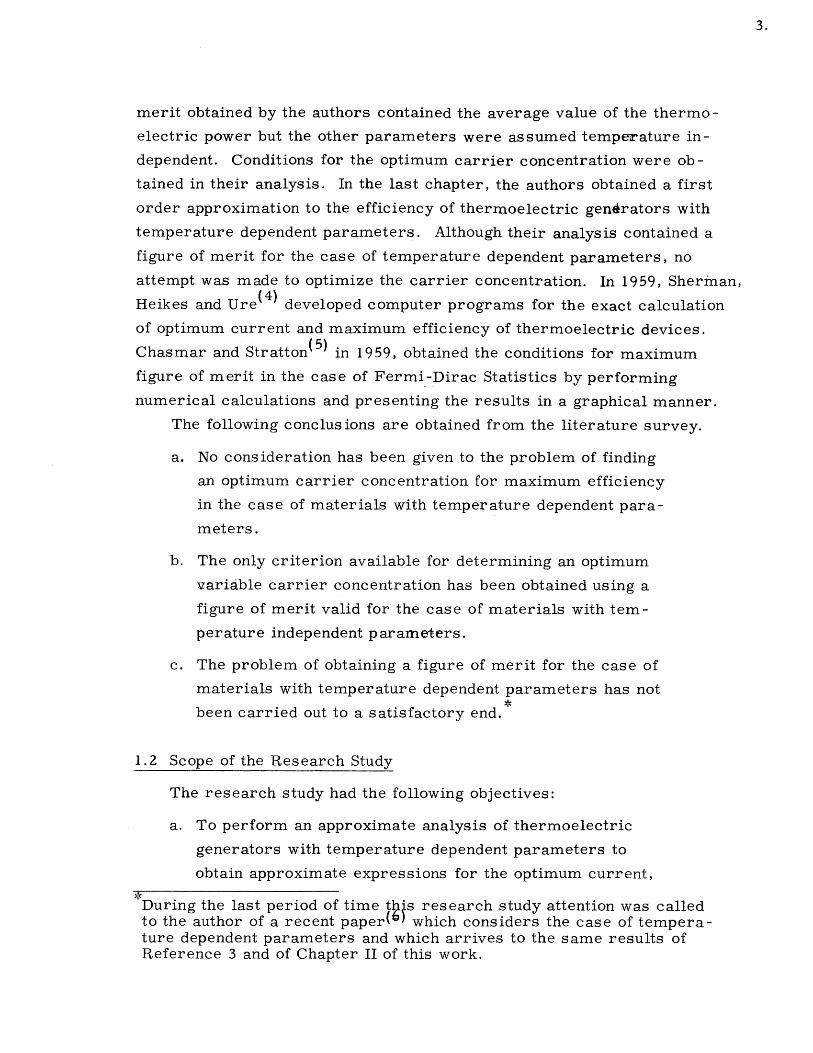
The following conclusions are obtained from the literature survey.

a. No consideration has been given to the problem of finding

an optimum carrier concentration for maximum efficiency

in the case of materials with temperature dependent para-

meters.

b. The only criterion available for determining an optimum

variable carrier concentration has been obtained using a

figure of merit valid for the case of materials with tem-

perature independent parameters.

c. The problem of obtaining a figure of merit for the case of

materials with temperature dependent parameters has not

been carried out to a satisfactory end.

1.2 Scope of the Research Study

The research study had the following objectives:

a. To perform an approximate analysis of thermoelectric

generators with temperature dependent parameters to

obtain approximate expressions for the optimum current,

During the last period of time t hs research study attention was calledto the author of a recent paper(v) which considers the case of tempera-ture dependent parameters and which arrives to the same results ofReference 3 and of Chapter II of this work.

4.

the maximum efficiency of the device, and a figure of

merit in terms of the material parameters. The ana-

lysis was carried out without restriction on the tempera-

ture dependence of the parameters.

b. To obtain general equations for the optimum constant and

variable carrier concentration in order to obtain maxi-

mum figure of merit. The equations had to be in general

form so that they could be applied to any semiconductor

model.

c. To apply the above equations to the case of a non-degenerate

extrinsic semiconductor. No assumption was made about

the band structure or temperature dependence of the para-

meters of the semiconductor.

d. To carry out an experimental program to verify the predic -

tions of part c on the optimum carrier concentration. The

verification was done by performing the necessary measure-

ments in a given material.

This report presents the results of these investigations.

1.3 Presentation of the Results

The results are presented in the same sequence as they were ob-

tained. The content of the report by chapter is as follows:

Chapter II: Expressions for the optimum current and maximum effi-

ciency are obtained for the case of temperature dependent parameters

by using a first order approximate solution to the heat conduction equa-

tion. A figure of merit is defined for the case of temperature dependent

parameters.

Chapter III: Equations are derived for the optimum carrier concentration

which yield a stationary value for the figure of merit. Conditions that are

mathematically sufficient are obtained for the stationary value to be a

maximum.

..- U -

5.

Chapter IV: Solutions of the equations for the optimum carrier concen-

trations are given for a non-degenerate extrinsic semiconductor. It

was assumed that the lattice thermal conductivity and the carrier mo-

bility were independent of the carrier concentration. The maximum

figures of merit for both constant and variable carrier concentrations

were compared.

Chapter V: The experimental program undertaken to verify the conclu-

sions of Chapter IV is repornted. The materials chosen for the experi-

mental program were n and p-type cast lead telluride. The procedure

for preparing the material by vacuum induction melting techniques and

the heat treatments necessary to produce uniform samples and to im-

prove the mechanical properties of the p-type material are described.

A detailed account is given of the apparatus used for measuririg thermo-

electric power, electric conductivity and thermal conductivity in the

range 300C - 275 0C. The experimental data are presented in graphical

form. The end of the chapter correlates the results obtained from the

theory in Chapter IV and the results deduced from the measurements.

Chapter VI: The general conclusions are reviewed and suggestions for

further work made.

CHAPTER II

EFFICIENCY WITH TEMPERATURE

DEPENDENT PARAMETERS

2.0 Introduction

The purpose of this chapter is to derive efficiency expressions

for thermoelectric generators with temperature dependent parameters.

Efficiency expressions are derived for the following two cases:

a. Thermoelectric generators with legs of similar

materials except for the sign of the thermoelec-

tric power.

b. Thermoelectric generators with legs of dissimilar

materials.

The principal assumption made in the derivations is that the tempera-

ture distribution along the legs is determined, to the first order of ap-

proximation, by the thermal conductivity of the material. This assump-

tion proves to be valid for thermoelectric generators but not for thermo-

electric coolers.

2.1 Efficiency with Temperature Dependent Parameters

The configuration pertinent to the analysis is shown in Fig. 2.1.

For this particular case, where both legs are of similar materials ex-

cept for the sign of the thermoelectric power, the efficiency of the de-

vice is the same as the efficiency n of one of its legs:

P0 (2.1)

where: Th P = power output = I adT -If2 O dx (2.2)

c

Q. = power input = Ia(Th )Th + Qh (2.3)

I = electric current

/LL/I/44/ "MATERIAL PARAMETERSa = ABSOLUTE VALUE OF THERMO-

P ELECTRIC POWERTYPE p = ELECTRIC RESISTIVITY

K = THERMAL CONDUCTIVITYCROSS SECTIONAL AREA A

Tc

Thermoelectric Generator with Legs of Similar Materials

Th MATERIAL PARAMETERS

~~ 2 a :,2 ABSOLUTE VALUE OFTHERMOELECTRIC POWER

2 TYPE PI'P2 = ELECTRIC RESISTIVITYK,,KL2 THERMAL CONDUCTIVITY

/. IICROSS SECTIONAL

AREA AiCROSS SECTIONAL

AREA A2

Fig. 2.2 Thermoelectric Generator with Legs of Dissimilar Materials

Qh = heat conducted at the hot end by one of the legs.

Qh =-(K A -) x=0

T = temperature.

The quantity of heat (Qh is determined by the heat conduction equationh

d(K.A ) + IT 12 = 0JR a-X ~ a-

with boundary conditions:

x= 0 T = Th ; x= I T = T,

Double integration of Eq. (2.4) and use of boundary conditions (2.5) give

the heat Qh the expression:

(2.5)

Th~cTQh" =d

fdxS ~A

dx xf Td 2

dxo KA

I f dx

dx

fo A

which can be written as follows:

Th dT TTh T f JThTdaQh h-Tc +I TC ThTda

h dT h dT-c T cc

2Th T71hPKdT hdT

_-2 Te c QI' dT

Th dT

fTc

where Q is defined as

Q= -KA

Substitution of Eqs. (2.2), (2.3) and (2.7) in Eq. (2.1) results in the

following expression for the efficiency of the device:

Th-Tc +IThdTT cq

dT

'Lh-LhdT Lhp KfhadT _fQ f-J-qdT

dT fdT

(2.4)

(2.6)

(2.7)

(2.8)

(2.9)

9.

where use has been made of Eq. (2.8) and of the identity:

T T

fThTda = aT - a(Th )Th + fTha dT (2.10)

Equation (2.9) is the expression for the efficiency of a thermoelectric

generator with temperature dependent parameters. It is valid for the

case of position dependent parameters as well as for the case of tem-

perature dependent parameters.

In order to evaluate the efficiency by means of Eq. (2.9) it is

necessary to know Q as a function of T and I. This dependence may be

found, at least in principle, from the solution of the heat conduction equa-

tion (2.4) and Eq. (2.8). Several authors have studied the solubility

conditions of Eq. (2.4) and have concluded that, in the most general case,

the solution cannot be represented in closed form. Therefore, in order

to carry the analysis any further without restricting the temperature

variation of the parameters, it is necessary to introduce an approxima-

tion for the evaluation of the efficiency. The simplest approximation

is to assume Q a constant:

Q Q = hKdT (2.11)c

An interpretation of this assumption is that the effects of the Joule heat,

Thompson heat and distributed Peltier heat upon the heat input are cal-

culated using the temperature distribution under no-load conditions.

This approximation is valid for thermoelectric generators but not for

thermoelectric coolers where the Joule heat distorts to a large extent

the no-load temperature distribution.

Substitution of Eq. (2.11) into Eq. (2.9) gives:

Th I 2 ThI adT- pKdT

c 0 c (2.12)

aTdT dT T adT 12 fhdTfhpKdTQ+I c + ICo AT AT Q AT

10.

where:

A T = Th - T (2.13)

Equation (2.12) is the first order approximation to the efficiency of a

thermoelectric generator with temperature dependent parameters and

has a form which makes it possible to find the optimum current for

maximum efficiency. The results of such optimization are as follows:

T

op cQ~~ T

0 1+M)hf pK dTc

(2.14)

AT.Emax 7h

(M+1)

M-1T T -T

aTdT fdT f a dT

c + c Thfh TIThf adT Thf adT

c c

T T

fThdT fjhpKdT

2 ,Th f pK dT

C

(2.15)

where:

T

( h adT) 2

M2=1+ TAT ST pKdT

c

Thf hadT

c

T TfhdT f adT

c

Thh adT

c

T TJdT f, PK dTc

T (2.16)

fhpK dT

The following changes in the order of integration:

T T T T TfThdT fadT = fadT f~ dT = f aTdT - Tc adT

c c c c c

T T T T T Tf, dT fh pKdT= fh p KdT f' dT = fTpKdT-Tcfh pKdT

c c c c c

(2.17)

11.

transform Eqs. (2.15) and (2.16) into:

ATEmax T~h

M - 1TdJh TadT

2(M+1) c Th

Th T adTc

T2f )ipKdT

hThJT pKdT

c

T -T T-

(f adT)2 ZThTadT fJTpKdT

M2 c c cATf pKdT L ShdT fhpKdT

c C. c c

Equations (2.14), (2.18) and (2.19) are similar in form to the equations

obtained with temperature independent parameters. The expression

(f hadT)2

c

AT T pK dTc

(2.20)

plays the role of figure of merit and the expression

2 Th TadT 4 TpxdT

C C

h h2f Ta dT f T pK dT

C CJadT f IpK dT

c c

(2.21)

plays the role of average temperature. A simple interpretation may be

given to Eq. (2.20) by multiplying both numerator and denominator by AT:

(2.18)

TS (M -1)

h

(2.19)

-- i-M - -

12.

fh 2 Th(fhdT) f adT a 2

c c 2 AT av (2.22)

h ThaAT f pKdT JTpKdT

c c

where the indicated averages are averages with respect to temperature.

This figure of merit using average parameters was suggested by Ioffe

but without any justification. It should be pointed out that there is not a

priori justification to consider expression (2.20) as the figure of merit

for the temperature dependent parameter case since the so-called

"average temperature" depends also upon the material parameters.

The only justification at this point of the analysis is the similarity of

the expression (2.20) to the figure of merit for the case of temperature

independent parameter. A more complete argument is presented in

Chapter III.

It is a surprising result that Eqs. (2.14), (2.18) and (2.19), which are

obtained by means of an approximation, give the right expressions for the

temperature independent parameter case. This "anomaly" in our results

can be explained as follows. One of the consequences of the approximation

expressed by Eq. (2.11) is to neglect the dependence of Q upon the current

I. If we take this dependence into account in the evaluation of the deri-

vative of Eq. (2.9) with respect to the current I, we find that the neglected

terms contain either of the following quantities as factors:

Th h_ a Th 1 aQ dT T Th a 8Q f h pK 8Q fh 18T 2 IdT, JT 2 aI dT, JT __ M dT (2.23)

cQ cQ cQ

These terms have the property that they vanish in the temperature in-

dependent parameter case. This property is shown as follows: Integra-

tion of Eq. (2.8) gives:

T dT4T K d (2.24)

c

Taking the derivitive on both sides of the above equation with respect

13.

to I, we obtain:

fhT 0

c Q(2.25)

This last equation is valid for any dependence of K upon T; in particu-

lar for K independent of T we obtain:

hl dT = 0c Q

(2.26)

From the above equation it follows that the expressions in (2.23) vanish

in the temperature independent parameter case.

2.2 Thermoelectric Generator with Legs of Dissimilar Materials

The configuration pertinent to the analysis is shown in Fig. 2.2.

We choose, without any loss in generality, leg 1 an n-type semiconductor

rod and leg 2 a p-type semiconductor rod. Many of the steps of the

analysis presented here are omitted since the development follows along

the same lines as the one presented in the previous paragraph.

The efficiency of the device, that is, the ratio of the power output

to the power input is given by:

ThI (a + a2)dT - Ic

AT

h dTcT2

TdT + fh

c

-hdT

c

fTjdT aT'a2 dT

+ c

hdT

cz

oth T Th ( I l)f hdT h dT

-12 c T Q dTL hdTf h dT

- Tc6

1~7=

AT

hdT

c 1

TTh dTf -q

Th (p d)2f h dT

2 QTfh dTTcT

(2.27)

14.

where Q and Q2 are defined as:

Q= -K A1 dT A T 2= 2 A2 ax

The numerator of Eq. (2.27) is the power output of the device and the

denominator is the power input. Introducing the simplifying approxi-

mations

A T

Q Q 1 0 T f KdT1 c

A T

Q2 Qzo 2r fhKdTa2 20 T2 d T2 c

and maximizing the efficiency with respect to the current I, we obtain:

I =

Th (a +a2 )dTc

TI (PK) dT

10 c

1+M

(2.28)

(2.29)

(2.30)T

+ 2 (1p)2 dTc

AT

max Th

M-1T

T(a 1 +a2 )dT

2(M+1) c -2

Thf h(al+a2)dTc

T1 hT(pK) dT+ 1

Thi Th ~Th Th

10 c 20 c

Tfh)

c C(M-1)h

pK) 2 I

(2.31)

where:

S+ d 2jTh(a + a 2)dT

To I

T2fThT(a+a,2)dT

c

AT Q0 +Qz1 fh( pK) 1 dT+ 1

c QZOT (pK) 2 dT]

2M = 1+

+a2 )dT

T TT I 1dT+ (p.K)20T

Qj- fT'(IPK)dT+-£TTpzd10 T 20 Tc

T Tfp(K)dT+ (pK)2dT

10c 20 c

We assume that the expression:

h(a + a2)dT2c I

AT (Q10+ Q20) [Q1Th

fT (pK),dT +c

(2.33)

(PK) 2dTI

CzO-

represents the figure of merit for this case. This choice is based upon

the similarity between expression (2.33) and the expression obtained for

the temperature independent parameter case. Expression (2.33) can be

maximized by a proper choice of the ratio Q10 to Q2 0.denominator in expression (2.33), we obtain:

T T Q2 Tfh (pK),dT + f (p K)2dT + QIf (p

c c '10 cK)1 dT+

Expanding the

Th(pK)2dT

Expression (2.34) reaches a minimum when

Q2o 2T

f h (pK) 2 dTc

f (pK) dT

Substitution of Eq. (2.28) into Eq. (2.35) gives the optimum ratio between

the areas and lengths of the legs:

T

fr,(pK)2dT

c

T

J hI dTc

ThT K2 dT

c

15.

(2.32)

(2.34)

(2.35)

(2.36)

16.

Substitution of the optimum ratio (2.35) into Eqs. (2.30), (2.31), (2.32)

and (2.33) gives:

Iop _

Th (ac

+ a2 )dT1

1+ M(2.37)

AT

Smax ThM - 1

ThT(a +a2 )dT

2(M+1) Tc

fh(a +a2)dTc

TfhT(pK)dT

-2 c

f h(pK),dTc

J (pK) 2 dTC

T- (M-1)h

(2.38)

T2 hT(a + a2)dT

Cf h

fT (al +a 2 )dTC

TfhT( pK)dT

c

h( pK),dTc

1

fTh pK)2 dT1+ c

fTh(pK),dTc

Figure of merit =

Tf hT(pK)2dT

C

fh (pK)dTc

(2.39)

f (a,+ a,)dT (a )+ (a) 2]2 av 2avj

'h ----- , T2a+ avK 2AT[ f,,h(p)1 dT fh(pK)2dT

c c4 ~

Equations (2.35), (2.37), (2.38) and (2.39) are the equations to the first

order of approximation for the optimum current, maximum efficiency

and optimum areas to lengths ratio of a generator with temperature de-

pendent parameters.

The last point in our analysis of the efficiency of thermoelectric

generators with temperature dependent parameters is to apply our equa-

tions to a particular solvable case. In this way, we may obtain an esti-

mate of the accuracy of our results. Sherman, Heikes and Ure4 have

2M = 1

17.

(2L.40U)

18.

developed computer programs for the calculation of the efficiency of

thermoelectric devices and have applied these computer programs to

some solvable cases in order to check their results. Here, we take

one of their cases and compare the exact results given by those authors

with the results obtained by our approximate analysis. The material

parameters of the example to consider are given in table 2. 1.

Table 2.1

Material Parameters

a p K A i

leg (pv/*C) (Q - cm) (watt/ cm 0 C) (cm ) (cm)

n -- 400 10 -5T T 110T

p 200 - 10T T

T = temperature in okelvin.

The cold and hot temperature of the device are 400 0, and 1500

respectively. The tabulation of the results obtained by means of Eqs.

(2.35), (2.37), (2.38), (2.39) and (2.40) is given in Table 2-2 together

with the exact values reported in reference (4)

Table 2.2

Comparison between exact and approximate values

Quantity Our Results Ref ence Error%

A (cm ) 4.47 4.50 -0.7%n

I (amps) 52.5 55.0 -5N

rmax(*/) 27.6 26.0 +6%

19.

1000

LULU

U

S500 -s ~

- --- P ARM (EXACT)- - - N ARM (EX ACT)

- o P AND N ARMS (OUR RESULTS)-0d\

~o 0.5 1.'0

Dx

NORMALIZED DISTANCE

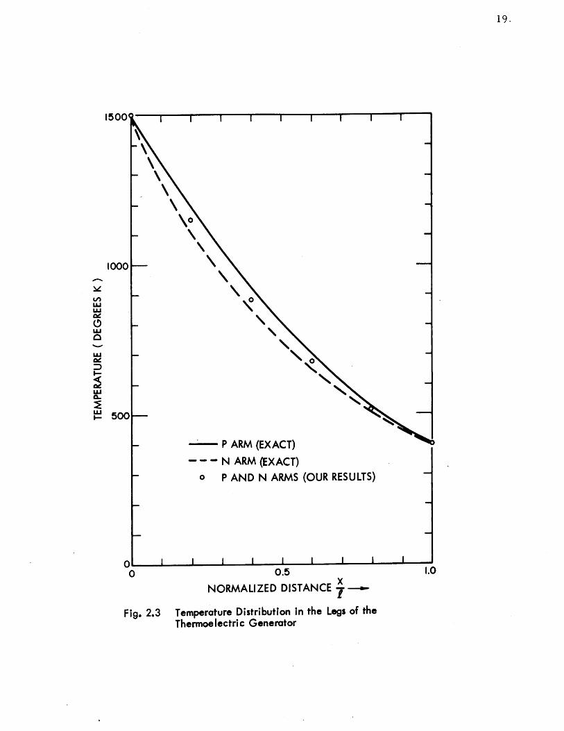
Fig. 2.3 Temperature Distribution In the Legs of theThermoelectric Generator

1500'

20.

The calculated values are in good agreement with the reported exact

values. The temperature distribution along the n and p arms calcu-

lated from Eqs. (2.29) and the temperature distribution reported in

reference (4) are shown in Fig 2.3. It is concluded that the flow of

current distorts in a small measure the temperature distribution under

no load conditions. The reason why the temperature distribution under

no load conditions falls below the exact temperature distribution for

the p arm and above the exact temperature distribution for the n arm

is next explained. In the p arm there is no Thompson heat, since the

thermoelectric power is constant; or in other words, the holes do not

exchange heat as they move from the hot source to the cold source

since their entropy remains constant. However, the Joule heat in the

p arm increases the temperature distribution above the temperature

distribution under no load conditions. The thermoelectric power in the

n arm has a lower absolute value at the hot than at the cold end. There-

fore, the electrons increase their entropy as they move from the hot

source to the cold source; this requires heat to be absorbed from the

material. This heat absorbed is larger than the heat generated by the

Joule effect and causes the temperature to fall below the temperature

distribution under no load conditions.

Conclusions:

In this chapter we have derived using first order approximation

the equation for the optimum current, maximum efficiency and opti-

mum area to length ratio of thermoelectric generators with tempera-

ture dependent parameters. We have shown by means of an example,

the accuracy of our equations. A figure of merit using average para-

meters has been defined. This figure of merit is used in subsequent

chapters for optimizing the thermoelectric properties of semiconduc-

tor materials.

21.

CHAPTER III

OPTIMUM CARRIER CONCENTRATION:

DERIVATION OF EQUATIONS

3.0 Introduction

The preceding chapter has shown that the efficiency of a thermo-

electric generator depends upon the material parameters a, p, and K.

It is well known that in semiconductor materials it is possible to exert

control upon these parameters by means of the carrier concentration

in the material. Even more, semiconductor materials can be produced

with carrier concentration constant along the length of the material, and

also with carrier concentration varying along the length . The determina-

tion of the optimum constant and optimum variable carrier concentra-

tion in order to achieve maximum efficiency is a very important tech-

nological problem in the application of semiconductors to thermoelec-

tricity. The purpose of this chapter is to derive the equations to be

satisfied by the optimum constant and optimum variable carrier con-

centrations in order to obtain maximum figure of merit. The reasons

for choosing the figure of merit as the quantity to be maximized are

discussed in Section 3.1 . The equations are obtained with a maximum

amount of detail for thermoelectric generators with legs of similar

materials. The equations for thermoelectric generators with legs of

dissimilar materials are given omitting some of the intermediate steps

in the derivation.

Before starting the discussion, we will introduce a simplification

in the writing of the equations. The limits of integration will be omitted

in all the integrals. It will be assumed that all the integrals are definite

integrals with limits of integration Th and T unless shown otherwise.

3.1 Figure of Merit as Quantity to be Maximized

For the matter of convenience, we restrict our discussion to the

case of thermoelectric generators with legs of similar materials. The

analysis in Section 2.1 indicates that the dependence of the efficiency

upon the material parameters is not as simple as in the case of tempera-

ture independent parameters. Equation (2.18) shows that the whole

efficiency expression, with the exception of the CaTrtot efficiency, de-

pends upon the parameters of the material. To consider Eq. (2.18) as

the expression to be maximized, would be a formidable task. The

quantity M is a better choice if it is shown that the efficiency is an

increasing function of M. We propose to do this next.

can be written:

M-1BM+C

where

fTadT cB= 2 Th1 adT T

,f TadTT

+h

The efficiency

(3.1)

(3.2)

(3.3)fTp KdT2 ThFp KdT

Taking the derivative of Ti with respect to M, we obtain:

dr7 _AT B+C

Th (BM+C)2

Equation (3.4) is non-negative as long as:

Th(B+C) = 2 2 fTadT fTpK dT 1> 0ThLfadT JpKdT

(3.4)

(3.5)

The interpretation to be given to the above equation is that the efficiency

is an increasing function of M as long as the average temperature, given

by Eq. (2.21), is positive. Condition (3.5) is satisfied if:

fa(2T - Th)dT : 0 (3.6)

which is valid for each of the following two cases:

a>0, daT? S0, Th > T (3.7)

(3.8)>O0, >ThT->,2>

c

Condition (3.7) is valid for a material used in the temperature range

AT

h

22.

23.

where the thermoelectric power increases with T. Condition (3.8) does

not set any restriction on the temperature depejdence of the thermoelec-

tric power, but sets a restriction on the ratio . Condition (3.8) is

always satisfied with the presently available materials. Since conditions

(3.7) and (3.8) do not impose any restrictions on the materials under

discussion, we conclude that the efficiency is an increasing function of

M.

Equation (2.19) shows that M is an increasing function of the product

of expressions (2.20) by (2.21). Therefore, maximum efficiency is ob-

tained when the product of the here called "figure of merit" by "average

temperature" is a maximum. It is important to notice the different way

in which the material parameters appear in the figure of merit and in the

average temperature. The figure of merit is the ratio of (aav)2 to (pK) av'In the average temperature we find the ratios:

(Ta) av (TpK) (9(a) ' (p K) av(3.9)

av av

where the dependence upon the material parameters seems to cancel. In

effect, let us consider the dependence of the above quantities upon the

carrier concentration n of a non-degenerate extrinsic semiconductor with-*

out electronic thermal conductivity. In this particular case:

a eC a - inn

(3.10)

n

Therefore, the average temperature becomes directly proportional to a

quantity of the form:

bd + b (3.11)

c -Inn

and the figure of merit becomes directly proportional to n. The weaker

dependence of the average temperature upon n favors the choice of the

figure of merit as the quantity to be maximized in order to obtain maxi-

mum efficiency. Without any further justification, we assume that the

figure of merit is the quantity to be maximized. For the matter of com-

pleteness, we derive in Appendix A the equations to be satisfied by the

*The material parameters for a non-degenerate extrinsic semiconductorare given in Chapter IV.

24.

constant and variables carrier concentrations in order to maximize the

product figure of merit by average temperature.

3.2 Equations to be Satisfied by the Optimum Carrier Concentrationin the Case of a Generator with Legs of Similar Materials.

Let it be assumed that a and p K are functions of the carrier con-

centration n as well as of the temperature T. We assume n to be an

independent variable constant along the material. The figure of merit

I becomes, then, a function of n:

I(n) = (fadT) (3.12)AT fpKc1'1

The optimum constant carrier concentration is determined by the

equation:

dI(n) = 0 (3.13)dn-

Performing the operation indicated in Eq. (3.13), we obtain

dI(n) 2fa a d - (a d)- fPK dT=0 (3.14)n ATfpKdT dT AT(fpKdT)2 an

which gives the following two equations:

f dT - C fa dT = 0 (3.15)

C = 1 fadT (3.16)

Since n and T are independent variables, we can write the above equations

as follows:

a(a ) a( pK)av - C av = 0 (3.17)

C = a v (3.18)1 av

25.

In order for Eqs. (3.17) and (3.18) to give a maximum, it is sufficient

that:

d2i < 0 (3.19)dn,

n = optimum

Taking the derivative of Eq. (3.14) we obtain:

d21 2a 1fdT- a 2 1~ 7 AT(pK) av -(K 2dTdn av Ln av an

2 a ta a av ftPKd 2+ a v a dT _ av LIpa dT (3.20)(AT) (pK) a n ( av

Evaluation of Eq. (3.20), as well as the solution of Eqs. (3.17) and (3.18),

cannot be carried out without knowing the explicit dependence of the

material parameters upon n. Equations (3.17), (3.18) and (3.19) are the

equations to be satisfied by the optimum constant carrier concentration.

In order to obtain the equations for the optimum variable carrier

concentration, it is necessary to use the techniques of the calculus of

variations. Let it be assumed that n is a function of T. This is not a

restriction since once we have found the concentration as a function of

T, we can find the no-load temperature distribution along the material

and obtain the dependence of the concentration upon the distance. Let

n('I) designate the optimum concentration which maximizes Eq. (2.20);

and let N(T) designate any other concentration given by:

N(T) = n(T) + E m(T) (3.21)

where e is a real number and m(T) an arbitrary function of T. Substi-

tution of Eq. (3.21) into a and p K makes Eq. (2.20) a function of c:

2I(E) = (fadT) (3.22)

AT J pK dT

26.

Since n(T) is by assumption the optimum concentration, I(E) must have

a stationary value at e = 0. Therefore:

I(e) 1E=O

= 0 (3.23)

Taking the partial derivative of I with respect to E, we obtain:

aJ(E) 2 fadT f-N mdT

Ie) AT fpKdT

Evaluation of Eq. (3.23) gives:

where

(fadT) 2

£ 8N mdTAT(fpKdT)(3.24)

(3.25)fadT aa CaPK)mdT = 0fpKdT- f-6-n an

C _ I fadT = aav

2 Ip dT 2~ (pK)av(3.26)

Since m(T) is an arbitrary function, it follows that:

aa C pK= 0an (3.27)

Equation (3.27) is similar to Eq. (3.17) without the averages. In order

for Eq. (3.27) to represent a maximum, it is sufficient that:

2 1a 2I(E)

aE Z E=O< 0 (3.28)

The expression for the second derivative of I with respect to E is:

2

a - =0

2aav a a 2 aav 2p K 2dTAT(PK) L an av an

+ 2 a mdT - av

(AT) (pK) an (pK)avaPK mdTJ' n I

(3.29)

27.

Equations (3.27) and (3.28) are the equations to be satisfied by the

optimum variable carrier concentration.

Before bringing to an end the discussion in this paragraph, we

obtain the equations for the carrier concentration which maximizes

the conventional figure of merit:

2z = (3.30)

pK

Taking the partial derivative of z with respect to n, we obtain:

28z = 2a aa a apK

n 2 n (3.31)I, (Kp)The optimum carrier concentration is given by:

- C' anK = 0 (3.32)

where:

C'= 1 a (3.33)Z pK

Equations (3.27) and (3.32) are similar except for the difference in the

factors C and C'. The quantity C contains the average values of the

parameters and the quantity C the point-values.

3.3 Equations to be Satisfied by the Optimum Carrier Concentration

in the Case of a Thermoelectric Generator with Dissimilar

Materials

Let it be assumed that the a's and 0 K's of legs 1 and 2 are func -

tions of the respective concentrations n and n2 as well as of the tem-

perature T. Then, the figure of merit given by Eq. (3.40) becomes a

function ofn 1 and n2:

2

fIa +a2dT1I(n 1 , n2) (a+az/l 2 (3.34)

AT [(pK) IdT+ f(pI+2 dij

28.

Let us consider first the case where n and n2 are constants along the

material and independent of T. The equations which determine the op-

timum values of n_ and n2 are:

aI(n ,n 2 ) =0 aI(n , n 2) =an 1 n2

Substitution of Eq. (3.34) into Eq. (3.35) gives the following two equations:

fC lxoni] dT = 0 (3.36)an 1a

aa a pK)?

fan2 - C2 an dT = 0 (3.37)

where

1 (a1 + a2 )dTC = I _ (3.38)

1 f(a +a 2 )dTC 2 y T -p -T+ (3.39)

The results indicate that the optimum carrier concentration of leg 1

depends upon the optimum carrier concentration of leg 2 and vice

versa. Furthermore, the carrier concentrations given by Eqs. (3.36)

and (3.37) are not the same as the carrier concentrations obtained

from solving Eq. (3.15) for each leg. The solutions are the same if and

only if:

a 1)a 2 av 2 (3.40)

p KJav 2 zlav

29.

The sufficient conditions for Eqs. (3.36) and (3.37) to represent a

maximum are given by:

2Z 2 8Ian 2 n 2 a n 1~an I an) a 2 < 0

an-

(3.41)a-I

7:< 0

Evaluation of the second order partial derivatives of Eq. (3.34) at the

optimum carrier concentrations gives the following results:

2

1 2 op

2f -dT -C f

an

82a2 K

ann1

(3.42)

dT

a 8(pK),dT 2f -dT - 2C1 a

(AT)2 [Y(pK) 1 a(pK) 2 a

21 2 a )av+ (a2 a 22dTCfan 2

dT AT Cp K) '+ 4/(27lF'22lop 1. av p 2 a 2

+- f dT -(AT) (pK) ~jaf 2 adT

2 pK)2an 2

Equations (3.36), (3.37) and (3.41) are the equations to be satisfied by

(3.43)

12dT J (3.44)

30.

the optimum constant carrier concentrations.

The equations to be satisfied by the optimum variable carrier con-

centrations are obtained by using similar techniques as in the calculus

of variations. Since the derivation follows the same procedure as the

one in the previous section, we merely state the results. The equations

which determine the optimum carrier concentrations are:

aa- a(pK) 1 = 0 (3.45)

a1 1an1

- C =? 0 (3.46)o-n 2 an

where C 1 and C2 are given by Eqs. (3.38) and (3.39). It follows from the

results that the optimum carrier concentration of leg 1 depends upon the

optimum carrier concentration of leg 2 and vice versa. The solutions to

Eqs. (3.45) and (3.46) are not the same as the solutions to Eq. (3.27) for

each leg unless Eq. (3.40) is satisfied. The sufficient conditions for

Eqs. (3.45) and (3.46) to represent a maximum are expressed by:

aI_)_ aI < 0 (3.47)a1 ae22 2 a2 1=0

-? 2=0

2 < 0 (3.48)

1 j E =0.. 1=0

where

2 = 0 (3.49)

1 2c e =0

- 2 =

31.

2

=0

2 2Sal 2 a(pK) 1 2f[7m dT -C f m dT

an-

2 dT2fp)1 2+ a dT - 2C f dT (3.50

(A&T) 2( 1p KT, a- 4M2 a 2 n11 an

82

ac2 E1 0E2 =0

- 22 a2 2 ) 2 2

f--m dT-C 2 f8 2 m dTan 2 an2 j

+ 2A)[~r ~f aa 2 mdT-2C2f a m dT (3.51)(AT) (pxav 2 j 2 n2,n

Conclus ions:

In this chapter we have obtained the equations to be satisfied by the

optimum carrier concentration which give a stationary value to the figure

of merit. We have obtained sufficient conditions for the stationary value

to be a maximum. The equations have been obtained in a general form

so that they can be applied to any particular semiconductor model. Two

important features of the equations obtained for the case of dissimilar

materials are as follows;

a. The optimum carrier concentration for material 1 depends upon

the material parameter of materials 1 and 2 (and similarly for optimum

32.

carrier concentration for material 2).

b. The optimum carrier concentrations for materials 1 and 2 op-

timized together do not correspond to the optimum carrier concentra-

tions for materials 1 and 2 optimized by separate, unless the figure of

merit of the materials are equal one to each other.

33.

CHAPTER IV

OPTIMUM CARRIER CONCENTRATION

SOLUTION TO THE EQUATIONS IN THE CASE OF

A NON-DEGENERATE EXTRINSIC SEMICONDUCTOR

4.0 Introduction

In Chapter III we obtained the general equations to be satisfied by

the optimum constant and variable carrier concentrations in order to

achieve maximum figure of merit. The explicit solution of those equa-

tions is not possible without knowing the dependence of the parameters

a, p, and K upon the carrier concentration n. The purpose of this

chapter is twofold.

a. To introduce the dependence of a, p, and K upon n for the case of

a non-degenerate extrinsic semiconductor.

b. To solve the equations of the optimum constant and variable

carrier concentration for the assumed semiconductor model.

The equations are solved for thermoelectric generators with legs of

similar materials. The model assumed for the semiconductor material

is the most general one.consistent with the conditions of being non-de-

generate and extrinsic, except for the assumption that the lattice com-

ponent of the thermal conductivity is independent of the carrier concen-

tration. Although the condition of non-degeneracy is somewhat restric-

tive, no attempt is made to carry out the analysis without this assumption.

Appendices B and C complement the discussion of this chapter. In Ap-

pendix B, the equations obtained in Appendix A are solved for a non-de-

generate extrinsic semiconductor with parabolic energy bands. In Ap-

pendix C, equations (3.26) and (3.27) are applied to a degenerate semi-

conductor using Fermi-DiTmi statistics, but no attempt is made to solve

them exactly.

4.1 Parameters of a non-degenerate extrinsic semiconductor:

The important parameters of non-degenerate extrinsic semiconduc-

tor are given by the equations:

n = Ne~r (4.1)

34.

a = (-)(s+rl)=( )(s+in ) (4.2)q q n

I - O'= nqp (4.3)p

K = KL +La-T (4.4)

where:

n = carrier concentration

N = total effective number of states

l = reduced Fermi-level (taken positive if it fallswithin the gap.)

s kI = average kinetic energy of the carriers.

p = mobility

K L = lattice thermal conductivity

= Lorentz number s( )2q

k = Boltzman constant

q = electronic charge.

It is assumed that 1, KL, and s are independent of the carrier concentra-

tion n. The parameters given by Eqs. (4.1) - (4.4) describe the proper-

ties of the semiconductor material as long as the following conditions are

valid:

a. The carrier concentration is determined by the number of impur-

ities and is independent of temperature.

b. The carrier mobility and the lattice thermal conductivity are

independent of carrier concentration.

c. The semiconductor material is in the non-degenerate range,;i.e.

Maxwell-Boltzman statistics tiS valid. Of these three conditions, the

last one is the most liable to be violated. However, removal of this as -

sumption brings the problem into the realm of numerical analysis.

It is pointed out that Eqs. (4.1)-(4.4) apply to semiconductors with

non-parabolic energy bands and to semiconductors where the shape of

the energy bands change with temperature.

If the semiconductor has parabolic energy bands, the values of N

35.

and s are given by:

N 2(27rm*KT)3/2 (4.5)h3

5S= 5+ X

where:

m* = density of states effective mass.

X = scattering parameter

h = Planck constant.

As a last part of this paragraph, we list some properties of Eqs. (4.1)-

(4.4) which will be used in the rest of the chapter:

aa _-k 1(4)-( ) (4.6)

(-) 2

an qn

2a a ~k. 1472 . = 2) L (4.9)an n

apK.... L (4.8)an n

2 p n2Lan n

n k PKL)l1a = a+ ( k)In 2 = a +( ) in (4.10)1 2 q n1 2 q FpK, T,

where a I and a2 are the thermoelectric powers of the respective concen-

trations n and n 2 . Equations (4.6)-(4.10) are a direct consequence of

the properties assumed for the semiconductor material.

4.2 Optimum Carrier Concentration in the Case of a ThermoelectricGenerator with Legs of Similar Materials.

Let us consider first the case of constant carrier concentration.

uu~a

36.

Substitution of Eqs. (4.6) and (4.8) into Eq. (3.15) gives:

f-()!dT +fadT fPKL dT = 0q n 2 JpKdT n(4.11)

Taking n out of the integrals and solving for (a) av, we obtain:

(a) = 2(k)av q

+ (LT)1L (PKL)avEquation (4.12) is the condition to be satisfied by the optimum carrier

concentration. Equation (4.12) can be solved for n in the following manner:

Let n be a constant carrier concentration with a thermoelectric a such

that:

(a ) = 2 k( )o av q

The relation between a and a is given by Eq. (4.10):

a = a +( k) in 00 q n

Taking averages on both sides of the above equation, we obtain:

k k n(a) = 2(k) + ( ) in -

av q q n

Substitution of Eq. (4.15) into Eq. (4.12) gives:

n 2(aT)in- o av

n (p 'av

since:

n0 (PK L)av

n pl o) tav

it follows that:

(4.13)

(4.14)

(4.15)

(4.16)

(4.17)

n n 2 (LT)av0 0

nin -= (pKlav

2(LT) avn

2 av

(4.12)

(4.18)

Equation (4.18) is a transcendental equation of the type

x in x = A (4.19)

nwhich can be solved for 0 as soon as n is known. The value of n is-_o -oobtained from substitution of Eq. (4.2) in Eq. (4.13):

In n = (s)av -2 + (in N)av (4.20)

Equation (4.18) can be written in the following equivalent form:

(pK )av in(pK )av 2(LT)avPL oa La L oav (4.21)

LyoP' EL)o]av 1J) pL)a

For the matter of completeness, the plot of Eq. (4.19) is given in Fig. 4.1.

In order to determine if the solution to Eq. (4.12) gives a maximum to

the figure of merit, the second derivative given by Eq. (3.20) is evaluated.

Substitution of Eqs. (4.6)-(4.9) and (4.12) into Eq. (3.20) gives:

d2I 2 26 T vd = - 2 1 + V < 0 (4.22)dn n (pL)av L Lav

Therefore, the figure of merit reaches a maximum. The expression for

the figure of merit at the optimum concentrate is given by:

k2-4( ) (LT)

(I) q 1 + av (4.23)o max (PK v L av

where it is understood that the quantities are to be evaluated at the opti-

mum carrier concentration.

Let us consider now the equations which determine the optimum vari-

able carrier concentration. Substitution of Eqs. (4.6)-(4.9) into Eq. (3.27)

gives:

k1 C L-()-+ C -=0 (4.24)qn n

Therefore:

PL= (k ) 1 = constant (4.25)

----- ---------

0.5 1.0 1.5

A

Fig. 4.1 Solution of the Equation XknX = A

38.

2.5

2.0

2.0

39.

Substitution of Eqs. (3.26) and (4.25) into (4.24) gives the following value

for (a)av

kI (LT) a(a) =2(-) + a 4.26)

av q PK

Equation (4.25) means that the temperature variation of the optimum

carrier concentration has to be such as to cancel the temperature vari-KL

KLation of the ratio -. For example, if the temperature variation ofp p

is of the type TP, then the optimum carrier concentration is of the type:

n = BTP (4.27)

where the constant B is determined by Eq. (4.26). In the particular case

of (LT) av= 0, the value of B obtained from substitution of Eqs. (4 27) and

(4.2) in Eq. (4.26) is given by:

in B = (s) av- 2 (in N) av p(in T)av (4.28)

The constant value of pK indicated by Eq. (4.25) be found as follows:

Let n be the constant carrier concentration defined by Eq. (4.13) and

given by Eq. (4.20). The relation between a and a. is given by Eq. (4.10):

k PKLa = a + ( ) in (4.29)

Taking averages on both sides of the above equation, we obtain:

(a)a= 2( )+( ) in p K - ( )fin(pKLdT (4.30)av q q L2T q Lo0

Equation (4.30) can be expressed in the form:

(a)a= 2( ) + (k) in _ L (4.31)av q q (TpK)

where:

in (pKL)= fln(pK dT (4.32)

40.

Substitution of Eq. (4.31) in Eq. (4.26) gives the following equation

for pK 2

pK pK- r L =

tT-ro FPKLo 0

2(LT) av

(~p~KL)o(4.33)

Equation (4.33) is of the same type as Eq. (4.19).VL The value of pK,7 from

Eq. (4.33) and the ratio - determine the optimum variable carrier con-qp

centration.

In order to determine if the solution given by Eq. (4.26) gives the

figure of merit a maximum value, it is necessary to evaluate the second

derivative given by Eq. (3.29). Substitution of Eqs. (4.6)-(4.9) and (4.26)

in Eq. (3.29) gives:

k 2 1= 2(-)

q PKavLaav-( q

2m-7Zn

dT av 2 mdT2+( -1)(f - )

(4.34)

By Schwartz inequality:

2mdT dT m dT 2

(f M 2d )(f d ) >: (f m d ) (4.35)

Therefore:

2Ii

a c=J E=u

k 2 1 aav_ -2(5) R (

av

m dT 2f n T) < 0

which indicates that the figure of merit attains a maximum value.

maximum value for the figure of merit is given by:

k24(-)

v ax q~1~ax P PKL

(LT)p avp"L

As a last point in this paragraph, we compare the maximum figures of

merit obtained with optimum constant and variable carrier concentrations.

(4.36)

The

(4.37)

E=O

aav-1) f

41.

For the matter of simplicity, we consider the case where:

(LT)av

KLo,- py1

= 0 (4.38)

(4.39)

The ratio between the maximum figures of merit is obtained from Eqs.

(4.23) and (4.37). After cancellation of the constant factors, we obtain:

v max

(ldmax

Bn

fT dTAT (4.40)

where B is given by Eq. (4.28) and n by Eq. (4.20). Subtraction of Eq. (4.20)

from Eq. (4.28) gives for the ratio B/n 0 :

in B = -p(in T)n av= finTdT

AKT

ThereforefinTdT

B

Substitution of Eq. (4.42) in Eq. (4.40) and evaluation of integrals gives

as a final result:

(Iv~max - _

(I ) x p+ 1c max

Tc

1 -

h

T T

p Th h

h (4.43)

The two limiting values of Eq. (4.43) are as follows:

(Iv)max

cI maxj

(4.41)

(4.42)

= 1

Tc

h

(4.44)

42.

(Imax(4.45)

C max

0h

The evaluation of Eq. (4.45) for several values of p is given in Table (4. 1)

Table 4.1

Evaluation of P

p p+11/2. 1.100

1 1.359

3/2 1.800

2 2.463

The results in the above table indicate that the larger the temperatureKL

dependence of upon the temperature the larger the gain obtained iny

figure of merit by means of variable carrier concentration. However,

the values given in Table 4.1 are for the limit condition of Tc /Th = 0.

The evaluation of the Eq. (4.43) for p = 3/2 and p = 2 as a function of

Th /Tc is given in Table 4.2.

Table 4.2

Evaluation of Eq. (4.43)

Th Eq. (4.43)

c p=l p=2_

1 1.000 1.000

1.5 1.035 1.050

3 1.050 1.185

The results of Table 4.2 show that for the usual values of Th/Tc there

is no appreciable gain in the figure of merit with variable carrier con-

centration over the figure of merit with constant carrier concentration.

- - 7, - -, - I Z"A

43.

4.3 Optimum Carrier Concentration in the case of a ThermoelectricGenerator with Legs of Dissimilar Materials

The analysis in this section is carried on with the additional assump-

tion that the Lorentz number is the same for both materials; other-

wise, the parameters of the materials are assumed to be different. We

follow the convention that subindex 1 and 2 refer to the respective ma-

terials 1 and 2. In view of the fact that the analysis in this seetion follows

very closely the analysis in section (4.2), many of the steps in the deriva-

tions are omitted.

To start the analysis, let us consider the case of constant carrier

concentration. Substitution of Eqs. (4.6) and (4.8) in Eqs. (3.36) and (3.37)

give the following two equations:

ClL(PKL1Ja - (L)A)T = 0 (4.46)

C2 [ 2Kav - () AT = 0 (4.47)

Substitution of Eqs. (3.38) and (3.39) in Eqs. (4.46) and (4.47) gives as a

result:

1pK)1 av OK) ]av (4.48)

or

[PKL av =[1K L)2av (4.49)

Equation (4.48) indicates that the optimum carrier concentrations are

such as to make (pK)av of the two legs equal. Let (pK)av and (pK L)avdesignate the respective values of Eqs. (4.48) and (4.49). Substitution

of Eqs. (4.48), (3.38) and (3.39) in Eq. (4.46) results in the equation:

(pKL) +(LT)(a av + (a 2) av4( L av av 4.50)

q (10L av

Equations (4.48) and (4.50) determine the optimum carrier concentrations.

The solution of Eq. (4.50) for (p0 ) is obtained as follows: Let (n )Iand (n 2 )o the constant carrier concentration be determindd by the conditions:

a )o av= 2( )L1~I av q[a o av

From Eq. (4.10) we obtain:

(n )a +a2 = (a) +(a2 ) + ( )In 1

1 2 1)+ q n1+ (!kS)In (n2)0

q (n )

Taking the average on both sides of the above equation, we obtain:

[[ (n1)O(n2Io(53(a )a+(a2av =a + (a2)1 v+ ( ) in n n2 (4.53)

Substitution of Eqs. (4.48) and (4.50) into Eq. (4.53) gives as final result:

(PKL) In (PK Lav

[PKL o av KL o av

(LT) av= 2

L~ o a0 Jv

PK L)J av PKL)1lav [IPKL)2 o av (4.55)

The carrier concentrations (n1 )o and (n2 )o are obtained from substitution

of Eq. (4.2) in Eqs. (4.51):

in(n )o = (s) av 2 + (in N )av (4.56)

in(N 2 o = (s) av 2 + (in N 2 )av (4.57)

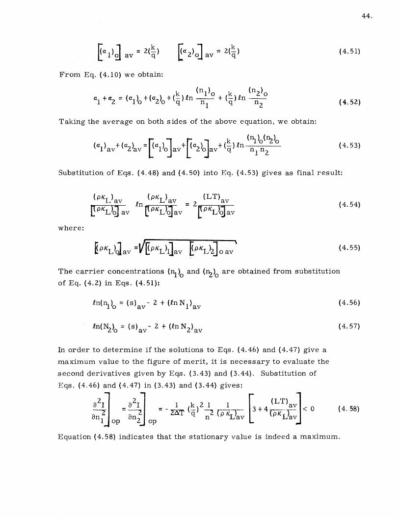
In order to determine if the solutions to Eqs. (4.46) and (4.47) give a

maximum value to the figure of merit, it is necessary to evaluate the

second derivatives given by Eqs. (3.43) and (3.44). Substitution of

Eqs. (4.46) and (4.47) in (3.43) and (3.44) gives:

821 2I12an1 op 2 op

I k 2 1 1~T

vn (pKL

F (LT)av3+4 (P LIav < 0

L- (pA

Equation (4.58) indicates that the stationary value is indeed a maximum.

44.

2(q (4.51)

(4.52)

where:

(4.54)

(4.58)

45.

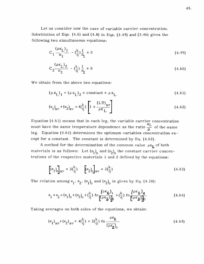
Let us consider now the case of variable carrier concentration.

Substitution of Eqs. (4.6) and (4.8) in Eqs. (3.45) and (3.46) gives the

following two simultaneous equations:

(KL) 1 k 1C1 n_ -)!i = 0 (4.59)1 1 qn 1

C -L ) =0 (4.60)2 n 2 q n 2

We obtain from the above two equations:

(p KL) 1 (PKL ) = constant = P KL (4.61)

k L (LT) avi(a1 ) + (a2 =4( ) + v (4.62)

Equation (4.61) means that in each leg, the variable carrier concentrationKL

must have the same temperature dependence as the ratio - of the same

leg. Equation (4.61) determines the optimum variables concentration ex-

cept for a constant. The constant is determined by Eq. (4.62).

A method for the determination of the common value pK of both

materials is as follows: Let (n)o and (n2 )o the constant carrier concen-

trations of the respective materials 1 and 2 defined by the equations:

a ) = 2 ( ) a2oa = 2 (k) (4.63)

The relation among a1 , a2, (a )o and (a2) 0 is given by Eq. (4.10):

(a)+a2+ (pKnf~) k (pKL (.4a +a =(a )o+(a ) +( ) In +( ) In (4.64)1 2 1 2 opKr)1) p" 20

Taking averages on both sides of the equations, we obtain:

(a ) +(a2 ) = 4( ) + 2( ) In (4.65)q q 2( pKq

WAS WAAU'

46.

where:

in(pKL)o = 1 [f Ip L)10 dT + fin[(pK L)} dT]

Substitution of (4.62) in Eq. (4.65) gives:

PKL nPK (LT)av_(n = 20

{ pKL) jo ( Y0j (pLjo

Equation (4.67) gives the value of p KL in terms of (K Jo. The expres -

sions for the carrier concentrations (n1 )o and (n2 )o are given by Eqs.

(4.56) and (4.57).

Finally, in order to determine if the solutions of Eqs. (4.59) and (4.60)

give a maximum value for the figure of merit, we perform the evaluation

of Eqs. (3.50) and (3.51). Substitution of Eqs. (4.6) - (4.59) and (4.60) in

Eqs. (3.50) and (3.51) gives the result:

E28E

2 _1 k 2 1

nC1 =0

2 =0

m2 dT

n

By Schwarz inequality:

(fm dT)2]-n )

fdT( m dT 2AT n T

It follows that:

2I 1 k2 1 1 av+21av= n (PKL) 2 k/q

e=02

(4.66)

(4.67)

1

(pK L)

m2 dT

(4.68)

(4.69)

V.13mdT 2

) IS<0

(4.70)

47.

We conclude that the solution represents a maximum.

Conclusions:

The principal conclusions that we can obtain from the analysis in

this chapter are as follows: For the semiconductor model assumed,

there are always optimum constant and variable carrier concentrations

which maximize the figure of merit. Although the model assumes the

semiconductor to be non-degenerate, the solutions for the average value

of the thermoelectric power [ 2()] show that this assumption may not

be valid. A characteristic of the solutions, is that the material parameters

enter as averages over the temperature range. This indicates that in

order to determine the relevant parameters for optimization purposes,

it is not necessary to perform a detailed evaluation of the material.

Direct measurement of the average value of the parameters for a sam-

ple may be sufficient. A possible method is suggested in Chapter VI.

Another very important conclusion is that variable carrier concentration

brings no improvement in the figure of merit obtained with constant

carrier concentration unless the ratio KL/p has a very strong tempera-

ture dependence and the ratio Th /Tc is larger than 3. Unfortunately,

these conditions are not met with presently available materials.

48.

CHAPTER V

EXPERIMENTAL PART

5.0 Introduction

It is the purpose of this chapter to report on the experimental re-

search program undertaken to verify the predictions of Chapter IV. A

detailed account is given of the procedure for the successful prepara-

tion of n-type and p-type cast lead telluride by means of a vacuum in-

duction furnace. Indication is given of the necessary heat treatments

on the n-type samples in order to obtain uniform materials and also on

the heat treatments of the p -type material in order to improve the

mechanical properties. A detailed description is given of the instru-

ments used for the measurement of the electric conductivity, thermo-

electric power and thermal conductivity, and of the tests performed on

the instruments in order to determine any anomalous errors. The re-

sults of the measurements performed on the cast samples in the tem-

perature range 300C - 2750C are reported and compared with the data

available in the literature. The thermoelectric properties of the n and

p type material are compared and plausible explanations are given to

account for the difference in behaviour.

The last part of the chapter correlates the results predicted by

Chapter IV with the results derived from the measurements. The op-

timum constant carrier concentration and the maximum figure of merit

obtained from the equations of Chapter IV are compared with the values

derived from the experimental data. The optimum variable carrier con-

centration is determined for the p -type material using the criterion of

Chapter IV. The figure of merit obtained using this carrier concentra-

tion distribution is compared with the figure of merit obtained with op-

timum constant carrier concentration.

5.1 Material Preparation

Lead telluride was prepared by direct reaction of high purity lead

(99.999%) and high purity tellurium (99.999%) in a helium atmosphere

49.

using a vacuum induction furnace. The vacuum induction furnace con-

sisted of a vacuum system with a cold trap, a reaction chamber, a

graphite crucible and an induction heating unit. The graphite crucibles

were machined from high purity graphite rod (A. E. C. grade). The

schematic diagrams of the reaction chamber assembly and graphite

crucibles are shown in Fig. 5.1. Inside of the reaction chamber there

was a stainless steel rod with a graphite tip at the end. This rod had

vertical movement inside the quartz tube and extended to the outside by

means of a teflon seal. The first step in preparing the material was

to remove the surface oxide from the lead and the tellurium. This was

accomplished with tellurium by vacuum distillation of the material and

with lead by surface etching with hydrochloric acid for 1/2 hour followed

by several rinses with hot water and hand drying with a lintless cloth.

The crucible containing the materials was capped and placed inside of

the reaction chamber and the whole system evacuated. With the vacuum

at 1 micron the system was flushed with helium. The helium was intro-

duced in the system through a valve placed before the cold trap and was

vented in a hood by means of the exhaust valve. After 2 or 3 cubic feet

of helium had passed through the system, the exhaust and helium inlet

valves were closed and the system evacuated again. Helium was again

admitted to the system when the vacuum reached 1 micron. Once the

system was filled with helium, the graphite crucible was closed with

the graphite tip and the reaction started. The crucible was heated by

the induction coil located around the reaction tube. The material was

reacted for 10 minutes at temperatures not less than 925 0 C and not

more than 950 0 C as measured by an optical pyrometer. After comple-

tion of the reaction, the power was turned off and the material quenched

in air. The material prepared by this method was polycrystalline with

large grains (4 mm long or more) and a bright appearance. The material

was not uniform due to a lack of mixing during the reaction. Because of

this fact, the material had to be crushed and then cast. The casting was

carried out in a second graphite crucible following the same steps as

in the reaction of the material. The cast samples were rods 1/2" in

diameter and 1 1/2" long. The samples obtained were uniform within

± 10% or better as determined by a thermoelectric probe. The proce-

dure explained above was used for both p and n type samples.

LESS STEEL ROD

TO VACUUM SYSTEMAND HELIUM INLET

- TO EXHAUST VALVE

O-RING SEAL

GRAPHITE -CRUCIBLE

NICKE L-PLATED--w COVER PLATES

QUARTZ TUBE

GRAPHITE TIP

0INDUCTION HEATING

COIL0

REACTION CHAMBER

HOLE

: z

CAP i-- -ETI

REACTING CRUCIBLE

HOLE

I |Ti i

i-4 - - n

CAP

CASTING CRUCIBLE

Fig. 5.1 Schematic Diagram of the Reaction Chamber Assembly and Graphite Crucibles

TEF

50.

SEAL

51.

The n-type material was prepared by using an excess of lead(7 ) over

the stoichiometric composition and by adding bismuth as impurity. The

ratio in weight of lead to tellurium was 1.6350. The bismuth was of high

purity (99.999%) and was used in the range of 0.027 to 0.4% by weight.

A ten hour annealing period at 800 0 C, using the same vacuum induction

furnace, gave samples uniform within ±5% as determined by a thermo-

electric probe. The p-type samples were obtained with a composition

rich in tellurium and by adding sodium as impurity. The ratio of Pb to

Tewas 1.6109 (. The high purity sodium (99.99%) was used in the range

of 0.003% to 0.076% by weight. The p-type samples obtained were very

uniform without additional heat-treatment. However, the p-type material

had very poor mechanical properties to the extent that it was not possible

to make cuts of less than 6 mm. The strong retrograde solubiliy exhibitedby the solidus line of the tellurium 8 ) indicated the possibility of age-

hardening the material in order to improve its mechanical properties.

The p-type material was slowly cooled from 8000C to room temperature.

The cooling time was around 11 hours. This heat treatment improved

the mechanical properties of the material. However, the p-type material,

especially the sodium rich samples, still did not show the same mechani-

cal properties as well as the n-type samples. This difference in the

mechanical properties of the n and p type material may be explained by

the difference in their composition. The n-type material had an excess

of lead which could precipitate in the grain boundaries. In the case of

the p-type samples, the excess tellurium was precipitated in the grain

boundaries giving a weaker bonding strength. This matter of improving

the mechanical properties of polycrystalline p-type lead telluride re-

quires further additional study. Perhaps an increase in the tellurium

excess or a better heat treatment could give the desired results.

Since the sodium is a very active material, it was stored in a jar

filled with kerosene. The material was cut under the kerosene with

help of a pair of tweezers and an x-acto knife. The material was

weighted in a weighting bottle containing kerosene. The change in

weight in the weighting bottle due to evaporation of the kerosene in the

process of removing its cap was found very consistent and of the order

a.tThis rationstoichiometry is 1.6237

52.

of 1/10 of a milligram. Once the sodium was weighted, it was placed

at the bottom of the reacting crucible adding a small amount of hexane

to cover the sodium and avoid oxidation. The other elements were

added to the crucible and placed inside the reaction chamber. The

hexane was boiled out in the process of evacuating the system. The

disadvantage of the hexane is that after several operations the oil of the

vacuum pump is contaminated. With enough practice in the assembling

of the system, it may not be necessary to use the hexane.

5.2 Thermoelectric Power and Electric Conductivity Measurements

Thermoelectric power and electric conductivity measurements

were performed on five n-type and five p-type samples of cast PbTe

covering the temperature range 300C - 275 0 C. All the samples had

different composition. The measurements were performed in a high-

temperature electric conductivity probe, already described in the litera-

ture, which was modified in order to allow for thermoelectric powermeasurements.

The modifications consisted of the addition of a small heater and a

thermocouple at the bottom contact. The sample holder was located

in a vacuum tight enclosure which allowed the measurements to be

carried out in a nitrogen atmosphere in order to avoid oxidation of the

samples. A schematic diagram of the system is shown in Fig. 5.2.

In this system the top and bottom contacts were stainless steel pressure

contacts with chromel-alumel thermocouples imbeded in them. The

thermocouple holes at the contacts extended a distance of 0.020" from

the surface. The thermocouples were electrically insulated from the

contacts with insalute cement. The current leads, which were also

used to measure the thermoelectric voltage, were stainless steel wire

0.010" in diameter and were spot welded to the contacts. The small

heater at the bottom contact consisted of 10 turns of No. 28 cupron wire

electrically insulated from the contact. The voltage contacts were

knife-like pressure contacts made from 0.010" thick nickel sheet.

These contacts were mounted in a piece of lava with a separation be-

tween the centers of the contacts of 4.06 mm. as determined by a

TOCONSTANTVOLTAGE

TRANSFORMER

VARIAC

zw A

SW0oz ~D <

VACUUM TIGHTENCLOSURE\ARIAC

A

I1S

Fig. 5.2 Schematic Diagram of the Thermoelectric Power and Electric Conductivity Apparatus

54.

micrometer. The leads welded to the voltage contacts were of 0.010"

diameter stainless steel wire. All the leads were brought out to a

switching box where by a proper switch arrangement, it was possible

to connect the thermocouple and thermoelectric power leads to a po-

tentiometer. By observing proper care in the electrical shielding of

the leads and in avoiding ground loops, the electrical noise level in

the system was better than 10 sv.To make satisfactory measurements in the equipment, it was neces -

sary to reduce the thermal resistance between the sample ends and the

sample holder contacts. To do this the sample ends were covered with

silver paint just before mounting. Once the sample was mounted, the

voltage contacts were set in place observing great care not to change

the position of the sample which could disturb the end contacts. The

voltage contacts were formed by discharging a capacitor between the

contacts and the sample. By this method, it was possible to obtain a

total contact resistance of less than 2 ohms. This procedure in the

mounting of the sample gave reproducible results of the order of ± 5%.

Sample sizes were on the average 8x2x3 mm. with the exception of

samples having a high electric conductivity in which case the area was

made smaller in order to avoid the use of a high current. The electrical

conductivity measurements were performed by measuring the current

which produced a voltage drop of 500 pv; with the exception of the high

electric conductivity samples which were measured with a voltage

drop of 200 pv. The current necessary to produce the required voltage

drop was below 200 ma. and the Joule heating of the sample did not

produce a temperature drift of more than a 1/4 0 C. Thermoelectric

power measurements were carried on by applying enough power to the

bottom contact heater to produce a temperature drop not less than 80 C

and not more than 10 0C. The temperature difference between the con-

tacts of the sample holder was always smaller than 1/4 0 C under equal-

ibrium conditions. This situation was obtained by a careful positioning

of the sample holder with respect to the ambient heater.

In order to determine possible errors in the measuring system,

some tests were performed as follows: a. All the n-type samples were

checked for reproducibility of the thermoelectric power measurement.

-- - Ooo MAIM,

55.

The samples were unmounted, the contacts cleaned and the sample

mounted again. The points reproduced were at the low, middle and

high ends of the temperature range. The reproduced values came

within ± 5%. b. In order to determine if the sample length affected

the thermoelectric power measurements, sample No. 19 was cut in

half and its thermoelectric power measured. The value came within

8% of the original measurements. c. Linearity tests were performed

on sample No. 19 of the voltage drop with current and of the Seebeck

voltage with temperature difference. The linearity tests were per-

formed at the low and high ends of the temperature range. Plots of

voltage versus current gave straight lines with non-zero crossings

of 1pv. The plots of Seebeck voltage versus temperature difference

were straight lines passing through the origin. Therefore, there were

no errors due to non-linearity. The estimated accuracy of our measure-

ments is as follows: Thermoelectric power measurements are esti-

mated to be withifll0%. It is very difficult to have an idea of the order

of magnitude of the contact thermal resistances. However, the fact

that our results reproduce within ± 5% lead us to the conclusion that

± 10% is a conservative value. The electric conductivity measurements

are believed to be within ± 10%. There are two sources of error in

this case: First, there is the determination of the length to area ratio.

Although the dimensions were measured with a micrometer, the non-

uniform shape of the cross Isection causes an error of the order of 4%.

Second, the voltmeter instrument (V.T.V.M. H.P.-400D) has a maximum

accuracy. The manufacturer specifies an accuracy of 2% at full scale,

which means, 4 or 5% at the middle of the scale. A voltmeter model

400H would have been a better choice.

The results of our measurements are given in Figs. (5.4) to (5.9).

The thermoelectric power is given with respect to stainless steel. A

discussion of these data is given in section (5.4).

5.3 Thermal Conductivity Measurements

The object of the thermal conductivity measurements was to

The thermoelectric power of stainless steel with respect to copperis 15 pv/ 0 C as measured by a thermoelectric probe.

56.

determine the lattice thermal conductivity KL and the Lorentz number

L for n-type and p-type cast lead telluride. This was accomplished by

performing the following two types of measurements: a. Measurement

of the thermal conductivity of an n-type and a p-type sample in the tem-

perature range 30 0C - 250 0C. b. Measurement of the thermal conduc-

tivity at 40 0 C of five n-type samples and three p-type samples. (The

samples used were taken from the same ingots as were the samples

used for electric conductivity and thermoelectric power measurements.)

The measurements were carried out in an apparatus described already

in the literature. 1 0 ) For completeness, a brief description of the ap-

paratus will be given. Fig. 5.3 shows schematic diagram of the thermal

conductivity apparatus. The apparatus consists of a bottom plate, the

sample, a top heater and a copper can. The space inside of the copper

can is filled with micro-quartz insulation.. The copper can is surrounded

by a heater to control the ambient temperature. The whole system is

located in a vacuum tight enclosure. Thermocouples are placed at the

top heater, the top end of the sample, the bottom end of the sample, the

copper base, the copper can and the ambient heater. The thermocouples

are platinum - platinum + 10% rhodium with the exception of the ambient

heater thermocouple which is chromel-alumel. The thermocouples are

brought out of the system through glass-to-metal seals to an ice-bath

and then to a switching box. The temperature of the ambient heater is

controlled by means of an automatic controller. At equilibrium condi-

tions, the temperature remains constant within a ± 1/4 0 C.

The samples used in the measurements were cylindrical rods 1/2"

long and 1/2" in diameter. Slots 1/2 mm. deep and 1/2 mm. wide were

cut at both ends of the samples to hold the sample thermocouples. The

sample thermocouples had glass insulation along their length, except

at the bead, to avoid short circuited paths. The procedure for mounting

the sample was as follows: The bottom contact was made first. The

bottom of the sample was painted with silver paint avoiding the silver

paint in the slot. The thermocouple, with a drop of silver paint at its

bead, was placed in the bottom slot and the sample pressed against the

bottom copper plate. The top contact was made in the same way.

To measure the thermal conductivity, the apparatus was calibrated

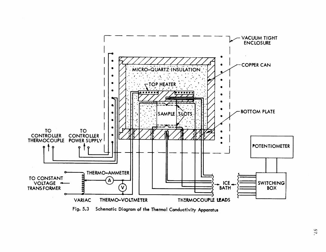
~~~ ~ VACUUM TIGHTENCLOSURE

TOCONTROLLER

THERMOCOUPLEtTO CONSTANT

VOLTAGETRANS FORMER

TOCONTROLLER*POWER SUPPLY

tL

THERMO-AMMETER- A

V11 1

*1 COPPER CAN

BOTTOM PLATE

MCRO-QUARTZ .IN SULATION-"

- OP HEATER-

.SAMPLE .5L6TS - -

- - 4 4 - - -L 0~~ TENTIOMETER

ICE., BATHi

2

VARIAC THERMO-VOLTMETER THERMOCOUPLE LEADS

Fig. 5.3 Schematic Diagram of the Thermal Conductivity Apparatus

PO

%.r-

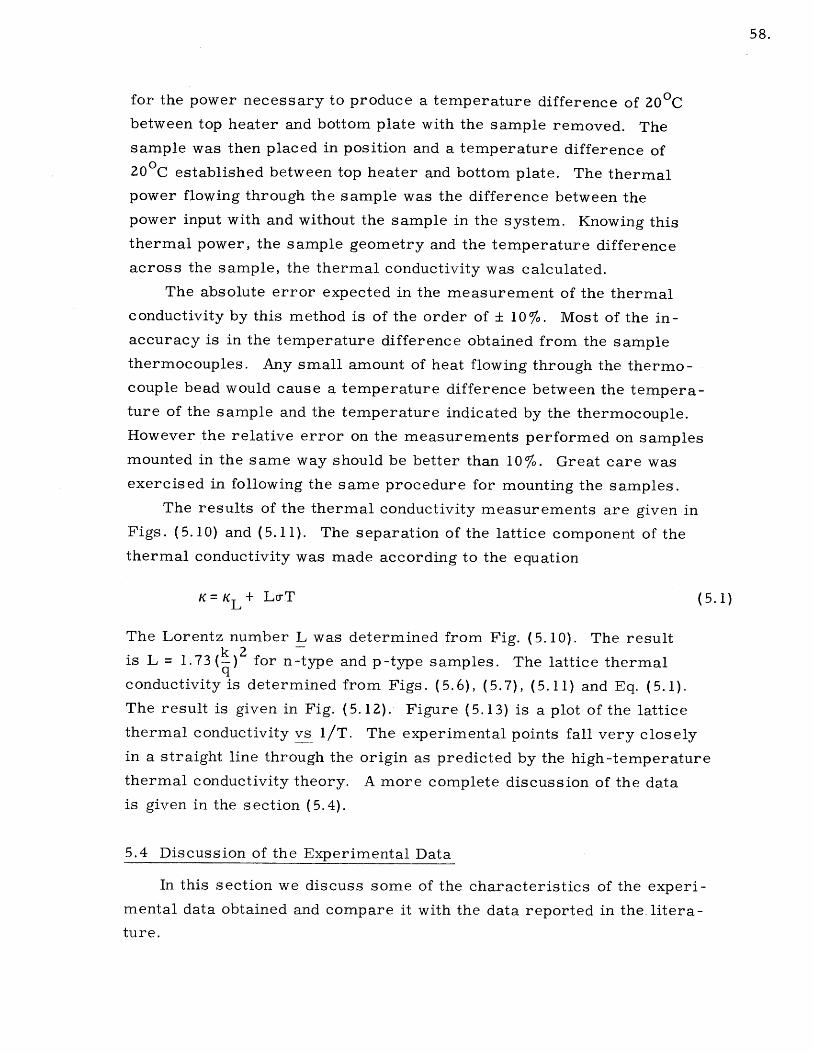
58.

for the power necessary to produce a temperature difference of 200Cbetween top heater and bottom plate with the sample removed. The

sample was then placed in position and a temperature difference of

20 0C established between top heater and bottom plate. The thermalpower flowing through the sample was the difference between the

power input with and without the sample in the system. Knowing this

thermal power, the sample geometry and the temperature difference

across the sample, the thermal conductivity was calculated.

The absolute error expected in the measurement of the thermal

conductivity by this method is of the order of ± 10%. Most of the in-

accuracy is in the temperature difference obtained from the sample

thermocouples. Any small amount of heat flowing through the thermo-

couple bead would cause a temperature difference between the tempera-

ture of the sample and the temperature indicated by the thermocouple.

However the relative error on the measurements performed on samples

mounted in the same way should be better than 10%. Great care was

exercised in following the same procedure for mounting the samples.

The results of the thermal conductivity measurements are given in

Figs. (5.10) and (5.11). The separation of the lattice component of the

thermal conductivity was made according to the equation

K= KL + Lo-T (5.1)

The Lorentz number L was determined from Fig. (5.10). The resultk 2-is L = 1.73( q) for n type and p-type samples. The lattice thermal

conductivity is determined from Figs. (5.6), (5.7), (5.11) and Eq. (5.1).

The result is given in Fig. (5.12). Figure (5.13) is a plot of the lattice

thermal conductivity vs 1/T. The experimental points fall very closely

in a straight line through the origin as predicted by the high-temperature

thermal conductivity theory. A more complete discussion of the data

is given in the section (5.4).

5.4 Discussion of the Experimental Data

In this section we discuss some of the characteristics of the experi-

mental data obtained and compare it with the data reported in the. litera-

ture.

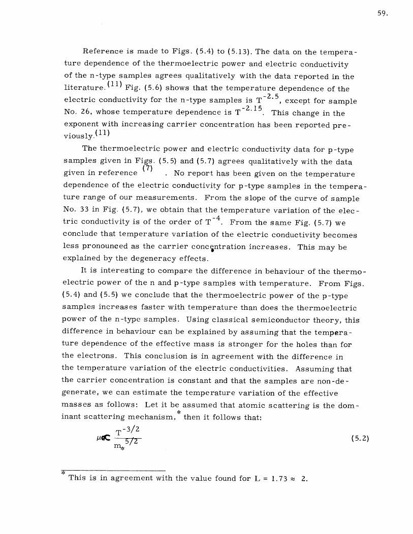
59.

Reference is made to Figs. (5.4) to (5.13). The data on the tempera-

ture dependence of the thermoelectric power and electric conductivity

of the n-type samples agrees qualitatively with the data reported in the

literature."" Fig. (5.6) shows that the temperature dependence of the

electric conductivity for the n-type samples is T 2.5, except for sample-2.15No. 26, whose temperature dependence is T . This change in the

exponent with increasing carrier concentration has been reported pre-

viously. 11)

The thermoelectric power and electric conductivity data for p-type

samples given in Figs. (5.5) and (5.7) agrees qualitatively with the data(7)given in reference . No report has been given on the temperature

dependence of the electric conductivity for p-type samples in the tempera-

ture range of our measurements. From the slope of the curve of sample

No. 33 in Fig. (5.7), we obtain that the temperature variation of the elec-

tric conductivity is of the order of T 4. From the same Fig. (5.7) we

conclude that temperature variation of the electric conductivity becomes

less pronounced as the carrier concgntration increases. This may be

explained by the degeneracy effects.

It is interesting to compare the difference in behaviour of the thermo-

electric power of the n and p-type samples with temperature. From Figs.

(5.4) and (5.5) we conclude that the thermoelectric power of the p-type

samples increases faster with temperature than does the thermoelectric

power of the n-type samples. Using classical semiconductor theory, this

difference in behaviour can be explained by assuming that the tempera-

ture dependence of the effective mass is stronger for the holes than for

the electrons. This conclusion is in agreement with the difference in

the temperature variation of the electric conductivities. Assuming that

the carrier concentration is constant and that the samples are non-de-

generate, we can estimate the temperature variation of the effective

masses as follows: Let it be assumed that atomic scattering is the dom-

inant scattering mechanism, then it follows that:

T -3/2P4C 5/2 (5.2)

This is in agreement with the value found for L = 1.73 ~ 2.

60.

400 i i i ia REPRODUCED POINTS 0 1

0 SAMPLE LENGTH CUT IN HALF

350 -

3002

0

0 22::L 250 -

0a-200 *29S200-

W26150-

N-TYPESAMPLE +19 - 0.027%IN WT OF Bi

100 -I #20 - 0.048% " "

#22 - 0.10 % " " "I

#29 - 0.24 % " " " "

-26 - 0.40 % s " " "

0 100 200 300

TEMPERATURE ( DEGREES C ) T

Fig. 5.4 Thermoelectric Power of N-type Cast Pb Te

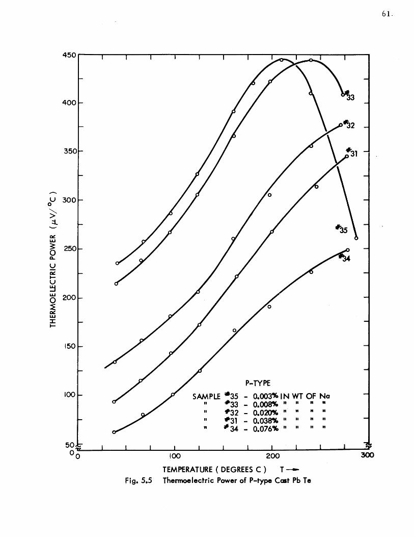
61.3

450-

400-

350-

U 300-0

3250-0C-

uL4

I0200 --

150

150-

P-TYPE100 - SAMPLE *35 -0.003% IN WT OF No

" *33 -0.008%""""" #32 -0.020%""""

- "t #31 -0.038% "1 "o " "sIN 34 -0.076% "f " 1 ""

50 10o 100 200 300

TEMPERATURE ( DEGREES C) T

Fig. 5.5 Thermoelectric Power of P-type Cast Pb Te

62.

500

2

300-

OU200--

20 0

b'100

50--~

30 --

300 350 400 450 500 550 60)

TEMPERATURE (DEGREES K) T -o

Fig. 5.6 Electric Conductivity vs Temperature for N-type Cost Pb Te

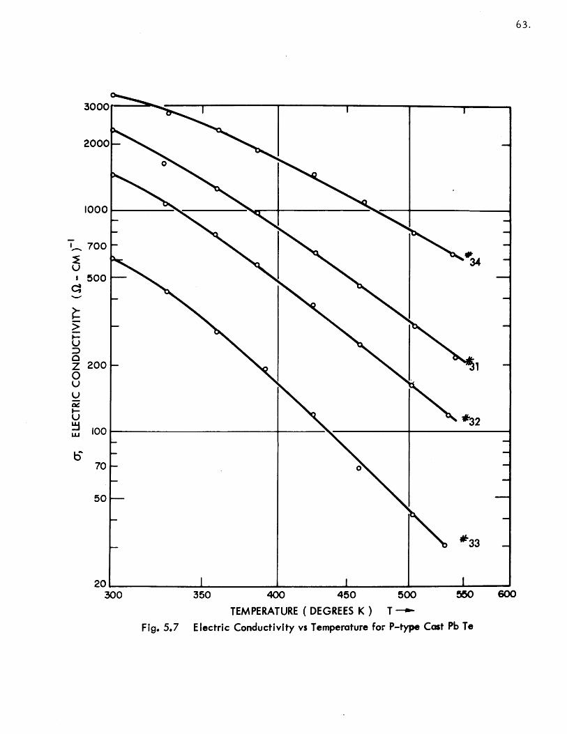
63.

3000-

2000--

10 0 0 - - - - - - - - -- - - - - - - - - - -- - -

700

IE 34-UI 500

C:

0Z 200-0UV

*32LU 100

70- -

50

033

?01300 350 400 450 500 550 600

TEMPERATURE (DEGREES K) T -

Fig. 5.7 Electric Conductivity vs Temperature for P-type Cast Pb Te

64.

0.02

19

0.01

.005 --

U 0 *22

I

C: 0

002- 29

'U

U0.001

U

.0005 -

.00021 1 t I

0 100 200 300

TEMPERATURE (DEGREES C) T-

FIg. 5.8 Electric Resistivity vs Temperature for N-type Cast Pb To

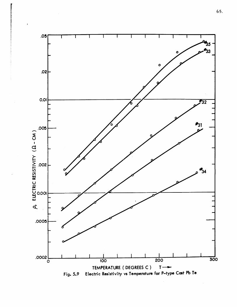
U

C:

> .002-I-

LLJU

U 0 .0 0 1LU

.0005T

0 100

TEMPERATURE (DEGREES C )Fig. 5.9 Electric Resistivity vs Temperature for P-type Cast Pb To

65.

T --

0-, ELECTRIC CONDUCTIVITY (91- CM)~Fig. 5.10 Total Thermal Conductivity ( 313 0 K ) as a Function of the Electric Conductivity ( 313 0 K)

25

20

15

0

E

z0

25

100

TEMPERATURE ( DEGREES C)

200

T

Fig. 5.11 Total Thermal Conductivity vs Temperature

201-

15F

0

E5

D

O

z0U

10-

51 -

010 300

SAMPLE #19 - N-TYPE

SAMPLE *35 - P-TYPE

I I * l I II I I-

100

TEMPERATURE (DEGREES C)Fig. 5.12 Calculated Lattice Thermal Conductivity vs Tempenrature (*C )

20

151-

I-

0

E

I-

z0

LU

Lu

5 k

101-

T -

-

I I I I I , I I I I I I I I I

-TYPE

P-TYPE

300

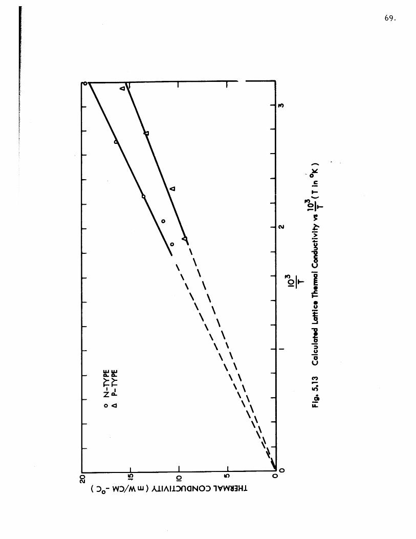
o -T

P

0 N

-TY

PEA

P-T

YP

E

-0*

20

0

15E st

0 0 z 0 U _j

5 0

-e

'00

-v-v

S I

I I

I I

I I

I I

I

T

Fig.

5.1

3 C

alcu

late

d L

attic

e Th

erm

al C

ondu

ctiv

ity v

0s (

T I

n OK

)

0-0

do

00:.

-

70.

From the above equation we obtain:

(m )nCT O.4 (n C T (5. 3)

where we have assumed that mobility of the electrons proportional to

T -2and the mobility of the holes proportional to T~4. However,

these conclusions need the support of Hall effect data. Next we discuss

our thermal conductivity data. Reference(12) reports a value of 2 for

the Lorentz number. This is in agreement with our value of 1.73 taking

into account inaccuracy in the measurements. With respect to the tem-(1 2)

perature dependence of the thermal conductivity, reference 2 reports

that above room temperature the thermal conductivity does not follow

the law 1/T. This result is in opposition to our measurements. However,

reference (13) has reported, by performing thermal diffusivity measure-

ments, that the thermal conductivity follows the law 1/T up to 250 0 C.

Since the results of reference (13) and our results were obtained by dif-

ferent methods and are in close agreement, we may assume the validity

of our measurements.

The data given in Fig. (5.12) shows that the lattice thermal conduc -

tivities for the n and p type are different at the lower end of temperature

range but become closer at the high temperature end. This difference

in the lattice thermal conductivity may be due to a difference in the struc-

tures of the materials. This assumption is supported by the fact that the

n-type samples were prepared with an excess of lead and the p-type sam-

ples with an excess of tellurium. Additional measurements performed

on samples prepared with different amounts of lead and tellurium are

necessary in support of this explanation.

5.5 Optimum Carrier Concentration

In order to compare the optimum carrier concentration for maximum

figure of merit predicted by the equations of Chapter IV with the one ob-

tained from our measurements, it is necessary to calculate the quantities

(a) av (pK Lav and (LT)av for a given temperature interval. We have

chosen the temperature interval 750C - 275 0 C. This is a reasonable tem-

perature interval for the operation of a thermoelectric generator. Fig-

ures (5.14) - (5.19) give the results of the calculations which were performed

400

"0

TEMPERATURE INTERVAL 750 C - 2754CS300- SAMPLES NO'S. 19, 20, 22, 26, 29

0

I--

U

0- 200-e PREDICTED OPTIMUM CARRIER CONCENTRATIONS

= 172 -U- --- N-LEG ALONE0I

- - P AND N COMBINED

100 -

I .

0 I | I I I | II I0 1000 2000 3000

0-, ELECTRIC CONDUCTIVITY AT 3000 K (g-CM)Fig. 5.14 Average Thermoelectric Power of N-type Cast Pb Te as a Function of Electric Conductivity

400

TEM

PER

ATU

RE

INT

ER

VA

L 75

*-

2750

C

SAM

PLE

NO

'S.

35,

33,

32,

31,

34-

30

0ce 0 I- U 2

200-

0 : 17

2

LU

PRED

ICTE

D O

PTIM

UM

CA

RRIE

R C

ON

CE

NTR

ATI

ON

S

P-LE

G A

LO

NE

P A

ND

N C

OM

BIN

ED

0I0

1000

20

00

3000

0;

ELEC

TRIC

C

ON

DU

CTI

VIT

Y

AT

3000

K

(,-

CM

)~

Fig.

5.1

5 A

vera

ge T

herm

oele

ctric

Pow

er o

f P

-type

Cas

t Pb

Te

as a

Fun

ctio

n of

Ele

ctric

Con

duct

ivity

300

200

0 20x r.30-

2

20-

10 26

7-

5

3

0 100 200 300

TEMPERATURE (DEGREES C) T

Fig. 5.16 pKL in (VOLTS) / *C vs Temperature for N-type Cast Pb Te

73.

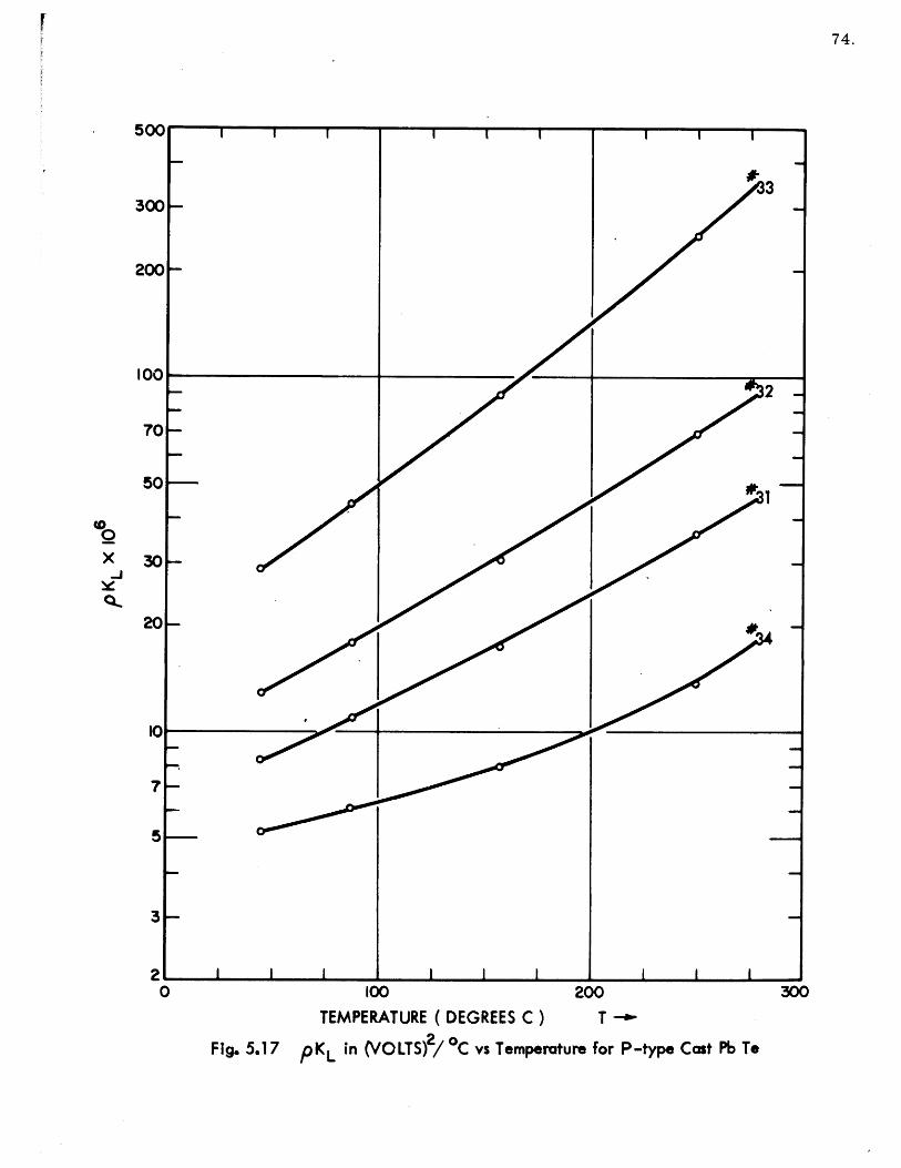
74.

500

3300

200-

1002

70-

50-

0

X 301

20-

170

5-

3-

2 I I I i

0 100 200 300TEMPERATURE (DEGREES C) T -+

2 oFig. 5.17 PKL in (VOLTS) / C vs Temperature for P-type Cast Pb To

WWWbNbNAlb-- - 1--- 1-1 - -- --- --- .

0, ELECTRIC CONDUCTIVITY AT 3004K (91 - CM) 1

Fig. 5.18 Plot of (pKL)v X 106 in (VOLTS) / *C vs Electric Conductivity for N and P-type Cast Pb Te

U-I

1000

x

Q,

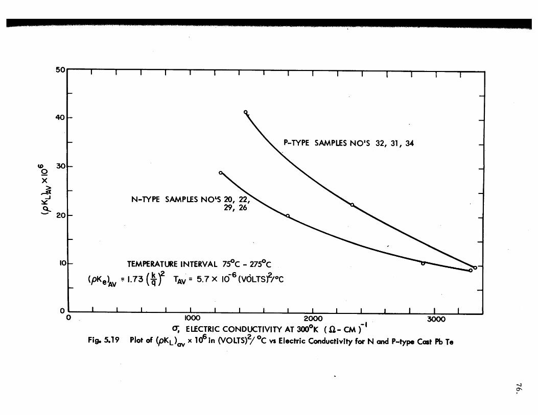
50 I I I I I

40

P-TYPE SAMPLES NO'S 32, 31, 34

N-TYPE SAMPLES NOLS 20, 22,29, 26

TEMPERATURE INTERVAL 750C - 2750C

(pKe)= 1.73 (if TAV = 5.7 X i0-6 (VOLTS)/OC

III - I I I I I . I I I I I I I I1000 2000 3000

0; ELECTRIC CONDUCTIVITY AT 3000 K (a- CM )'Fig. 5.19 Plot of (pKL)ao X 1O6 in (VOLTS) 2/ *C vs Electric Conductivity for N and P-type Cast Pb To

30k0x

20-

101-

I50 I I I I I I I I I I I I I I I I

2.0

P-TYPE

N-TYPE

1.50

1 .0-t - II I I I I I I I I I I00 1000 2000

q; ELECTRIC CONDUCTIVITY AT 3000K (I - CM)Fig. 5.20 Average Parameters Figure of Merit as a Function of Electric Conductivity

78.

by using numerical integration using Simpson's rule. Figure (5.20)

shows a plot of the figure of merit for n and P type samples as a func -

tion of the room temperature electric conductivity. The optimum values

for the room temperature electric conductivities as determined from

Fig. (5.20) are:

(- )op = 1250 (Q - cm) (5.4)

(c- ) = 2700 (0 - cm)

The optimum values predicted by Eq. (4.21) are obtained as follows.

From Figs. (5.14) and (5.15) we obtain a- for (a )a=Zr() = 172piv/ 0 C:-o oav q

(ono = 2520 (Q -cm) (5.5)

(o )o = 3340 (Q - cm)

The values of (pKL)o av from Figs. (5.18) and (5.19) are:

{ pKL) av = 13.25 x 10 6 volt2 / C (5.6)

£L( PKLp av = 9.5 x 10 volt / C

Therefore:

2 (LT)av _ 2x5.7

p KL no av 13.25

2(LT)av 2 x 5.7

{pKL)p o} av

From Eq. (4.21) and Fig. (4.1) we obtain:

(p KL optimum = 222 x 10 6 volts 2/ oC (5.8)

-6 2o(DKTV~ 18.0OxlO0 volts P C

LIp optimum

79.

From the above values and Figs. (5.18) and (5.18), we obtain:

(n optimum

(p)optimum

= 1650 (Q -cm)~

= 2650 (Q - cm)-

These values should be compared with the values given in (5.4).

(5.9)

The

error in the predicted n-type concentration is of the order 30%. The

error in the predicted p-type concentration is of the order of 2%.

The predicted maximum figures of merit by Eq. (4.23) are:

(Ic n max -3 o ) -l=1.63 x 10 (K (5.10)

(Ic) ma = 2.16 x 16-3 (ox) -

The maximum figures of merit corresponding to (5.4) are:

(Ic nmax = 1.96 x 10-3 (oK)-

(Ic p max

(5.11)

= 2.01 x 10 3 (o -1

We summarize the results in Table (5.1).

Table 5.1

Comparison between predicted and actual values

The largest error obtained is for the n--type sample. This is explained

by looking to the plot of the thermoelectric power n temperature in

80.

Fig. (5.4). The data of Fig. (5.4) shows that the n-type sanmples weremore degenerate than the p samples. The agreement for the p-type

samples is excellent. Although the predictions for the n-type samples

are inaccurate, it is important to notice that if the predicted concentra-

tion were used, the true figure of merit would be 1.84 x 10 -3 O) - as

obtained from Fig. (5.20). We discuss next the case where the n and p

legs are optimized simultaneously. In order to determine the optimum

concentrations from the experimental data, it would be necessary to

have a three-dimensional plot of the figure of merit given by Eq. (3.34)

as a function of Yn and a- . However, from Fig. (5.20) we conclude that

both materials have the same maximum figure of merit and therefore

the optimum concentrations should be very close to the concentrations

(5.4).- On this basis we compare the solution given by Eq. (4.55). The

results of the calculations are given in Table 5.2.

Table 5.2

Simultaneous Optimization of n and p material

Theory Experiment Error %(Eq. 5.4)

*p n 1800 1250 +43%

opt.

(Q-cm)~ p 2500 2700 -7.3%

I 1.90x10- 3 1.98x10 3 -4%max

(OK)

* Measure at 300 OK

The error in the predicted concentrations is large. However, the error

in the figure of merit is acceptable. The reason for a better agreement

in the figure of merit in this case, may be due to a very flat maximum

in the figure of merit when both materials are optimized together.

As a last case in the check between the theory developed in Chapter

IV and the experimental results, we consider the case of optimum vari-

able carrier concentration for p-type lead tebluride. We do not consider

81.

n-type material because by our previous calculations we arrived at the

conclusion that the p-type material satisfies more closely the model of

semiconductor postulate in Chapter IV. The optimum variable carrier

concentration is given by Eq. (4.33). In order to solve this equation, it

is necessary to know the value of (K ) . The value of this quantity is

obtained from Eq. (4.32). The evaluation of Eq. (4.32) is done as follows:-1

From Fig. (5.15) the value of T is 3300 (0-cm)-. With this value and

with help of Fig. (5.21), we obtain (pKL o as a function of temperature.

Performing the integration indicated in Eq. (4.32), we obtain:

(KL)o = 9.05 x 10 (volts) / C (5.12)

Using this value in Eq. (4.33) we obtain:

(p K ) . = 17.4 x 10- 6 (volts)2 / C. (5.13)L optimum

This value is indicated in Fig. 5.21. The above value of (p KL) determines

the dependence of the optimum variable carrier concentration upon tem-

perature. This dependence is shown in Fig. 5.23 which was obtained with

the help of Fig. 5.21. For the matter of comparison, the optimum con-

stant carrier concentration is shown in the same Fig. 5.23. Evaluation

of the predicted maximum figure of merit according to Eq. (4.37) gives

the following result:

-30 -1(IV)max = 2.25 x 10 - K) (5.14)

The relation between the maximum figures of merit obtained with variable

and constant carrier concentrations is given by:

(Ivmax - 2.25 = 1.04 (5.15)(I ) - 2.16c max

The value of (I ) was obtained from Table 5.1. The value given byc maxEq. (5.15) falls within the limits predicted by Table 4.2.

It is interesting to calculate the actual figure of merit which could

be obtained with the optimum variable concentration. This calculation

82.

500 7 0C |.05X | 2

275*C (p0KL)=9.05 x0 (VOLTS)2/*C

250 0C (p KL) 17.4 X 1c6 (VOLTS) 2/oC

200 2250C

200*C

17540C100

-1 50*C

~125*0C

50 -100*C -

(000 - 75*C-x

~ (p KL)O

20-

10

0 500 1000 2000 30000; ELECTRIC CONDUCTIVITY AT 300K ( - CM )

Fig. 5.21 pKL x 106 in (VOLTS)/ *C for P-type Cast Pb Te at Constant Temperatureas a Function of Electric Conductivity at 3000 K

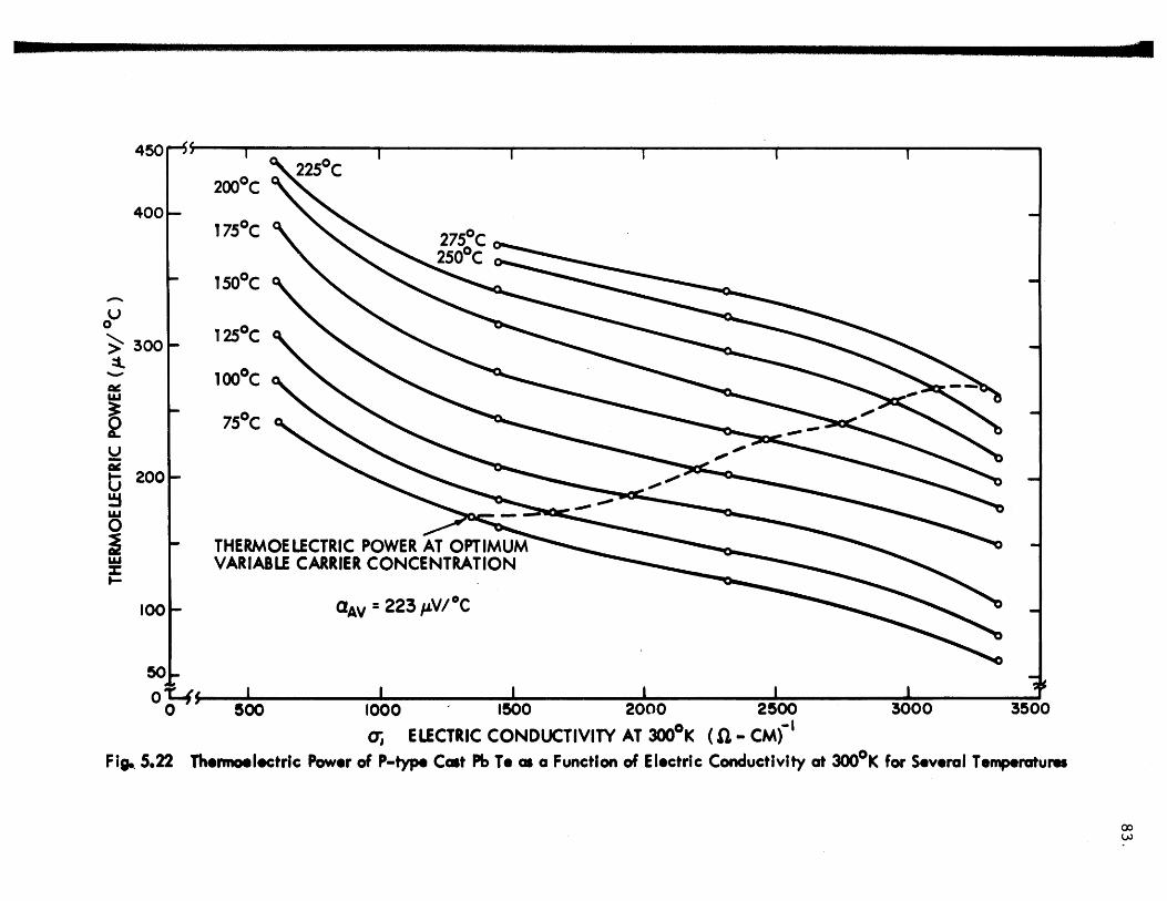
I I I I I

2000C

1750C

~ 1500C

- THERMOELECTRIC POWER AT OPTIMUMVARIABLE CARRIER CONCENTRATION

|000I I I

2000 2500

(l- CM)-500

a; ELECTRIC CONDUCTIVITY AT 3000KFig. 5.22 Thermoelectric Power of P-type Cast Pb To as a Function of Electric Conductivity at 3000 K for Several Temperatures

450-r

400F-

300 1- 1250C

1004C

750C

LU0

2U4IM

0

200 I-

100 1-

rf09

500 3000 3500

4

1

I

0

a0 ,

Lu

84.

3500

:3000

OPTIMUM CONSTANT CARRIERCONCENTRATION

2500-

D 2000 -z0

U1500 - OPTIMUM VARIABLE CARRIER CONCENTRATION -LU

-- "V!) =x 1.04

1000- (Ic)m

00 100 200 30

TEMPERATURE (DEGREES C) T-+-

Fig. 5.23 Predicted Optimum Carriers Concentration for P-type Cast Pb Te

-U

85.

is done by means of the equation:

2(a

av-(pC) av(5.16)

Since the carrier concentration is such as to make pKL a constant, itfollows that:

(pKa) + + LT 17.4 x 10 +5.7 x 10 6 = 23.1 (volts)2 /oC(5.17)x 10 6

The value of (a)av for this optimum variable carrier concentration is ob-tained with the help of Figs. (5.21) and (5.22). Performing the numericalintegration, we obtain:

(a)av = 223 pv/0C

Therefore, the figure of merit (5.16) has a value of:2

(a)-3o-(P )av = 2.16 x 10 3 (0K-1 (5.18)(P p K1av

This value should be compared with the value 2.01 x 10 -3 obtained fromTable 5.1. The increase in figure of merit is 7%.

5.6 Analysis of the results and conclusions

Before discussing the results, it is convenient to define the meaningof the terms degenerate and non-degenerate. We will define degenerateto mean that the Fermi-level is within the band and non-degenerate tomean that the Fermi level is within the gap. In the case of our material,where we found a Lorentz number of approximately 2 (i.e. atomic scat-tering), the material is non degenerate when the thermoelectric poweris larger than 2( ) and degenerate when the thermoelectric power isless than 2( ).

qFrom Figs. (5.4) and (5.5) we can conclude that the p-type samples

are less degenerate than the n-type samples in the temperature range

The value of 2( ) is 172 Pv/ 0 C.q

86.

0 075 - 275 C. The reason for this is the large increase in the thermo-electric power with temperature in the case of p-type material. Forexample, samples No. 34 and No. 26 start with, approximately the sameFermi-level at room temperature; sample No. 34 becomes non-degenerate

0at a temperature of 175 C, however, sample No. 26 always remains inthe degenerate region. This difference in behavior was explained on thebasis of tetemperature dependence of the effective mass larger in thep-type than in the n-type. Another important difference is obtainedfrom Figs. (5.14) and (5.15). From those figures we concluded the (a)k avfor the p-type samples was always larger than 2( ). For some of the

qn-type samples this condition was not satisfied.

I. Having in mind the above remarks we can arrive at the followingconclusion from table 5.1:

la. For materials which demain slightly degenerate, theEqs. (4.12) and (4.21) give good results with errorsbetter than 10 %.

lb. For materials which remain medium degenerate, theEqs. (4.12) and (4.21) give errors of 40 % in the car-rier concentration and of 20% in the figure of merit.The value predicted for the figure of merit is alwaysconservative.

1c. The actual figures of merit obtained with the predictedcarrier concentration are within less than 8% of themaximum figures of merit. This is due to the flatnessof the curve of the figure of merit n carrier concentra-tion at the optimum carrier concentration.

ld. The larger the temperature dependence of the effectivemass with temperature, the better the agreement be -tween the predicted values and the actual values.

le. If the temperature dependence of the effective mass isT, the errors are better than 10%.

I f. If the temperature dependence of the effective mass is1/2T ,the error in the carrier concentration is within

87.

20% and the error in the figure of merit is within 4.%.

II. From the results of Table 5.2 we can obtain the following conclusions:

2a. If one of the materials is slightly degenerate andthe other medium degenerate, then the error in thefigure of merit, in the simultaneous optimization ofboth materials, is less than 10%. This conditionoccurs because the flatness of the curve of the figureof merit versus concentration increases when bothmaterials are optimized together.

III. With respect to the case of Variable carrier concentration we canstate the following conclusions:

3a. For the case of a material which remains slightly degenerate,the value of the ratio of the figure-of merit at optimum vari-able carrier concentration to the figure of merit at optimumconstant concentration is within the predicted values.

3b. For materials which are medium degenerate even if thefigures of merit are in error by 20%, the ratio of themwill partially compensate the errors and give resultswithin the predicted values.

88.

CHAPTER VI

CONCLUSIONS

6.0 Introduction

The general conclusions of this research study are divided into

two parts:

a. The conclusions obtained from the analytical

study.

b. The conclusions obtained from the experimen-

tal verification of the analytical results.

6.1 Conclusions from the Analytical Study

An exact expression for the efficiency of thermoelectric generators

with temperature dependent paramters can be written with the help of a

repeated integration of the heat conduction equation. Exact evaluation

of the expression for the efficiency cannot be carried out without the

solution of the heat conduction equation. In the general case theheat con-

duction equation cannot be solved in closed form. Evaluation of the ef-

ficiency expression is possible by assuming that the temperature distri-

bution in the material is given to a first order of approximation by the

no load temperature distribution. Assuming this approximation to be

valid, the equivalent internal resistance of the generator is equal to the

equivalent internal resistance under no load conditions and the amount

of heat supplied at the hot source is equal to the heat conducted through

the material under no load conditions minus the Joule and Thompson

heats returned to the hot source, calculated for a temperature distribu-

tion equal to the no-load temperature distribution.

The approximate expression for the efficiency can be optimized with

respect to current. The expressions for the optimum current and maxi-

mum efficiency have the same form as in the case of temperature inde-

pendent parameters. An important property of the approximate expres -

sions is that they reduce to the exact expressions in the case of tempera-

ture independent parameters. This "anomaly" was explained to be a

89.

consequence of a general property of the quantity of heat flowing

through the material.

Application of the approximate equations to an exact solvable

case gave errors less than 10% in the values of the optimum current,

maximum efficiency and optimum area to length ratio.

The approximate efficiency expression is an increasing function

of the quantity:

2 (fadT) 2faTdT _FpKTdTM - =j APpKdT adT -pKdT (2.19)

The first factor is interpreted as a figure of merit with average para-(a) 2meters (- -3v and the second term in brackets interpreted as an average

Pavtemperature.

The problem of finding the optimum value of a material variable in

order to obtain maximum efficiency is eqUivalent to the problem of finding

the value of the material variable which maximizes Eq. (2.19). In the

particular case in which the material considered is a non-degenerate ex-

trinsic semiconductor and the material variable is the carrier concentra-

tion, the dependence of the average temperature upon the carrier concen-

tration is weaker than the dependence of the figure of merit upon the

same variable. The error committed in neglecting the variation of the

average temperature upon the carrier concentration in maximizing'Eq.

(2.19) with respect to the carrier concentration is of the order of 104/

for Th /Tc < 2. Therefore, to the first order of approximation, the pro-

blem of finding the optimum carrier concentration in a non-degenerate

extrinsic semi-conductor for maximum efficiency is reduced to the

problem of maximizing the expression:

2

(fadT) 2 a (2.20)AT( pmdT) ( pK)

av

with respect to carrier concentration.

In the case of thermoelectric generators with legs of similar

90.

materials, the equation for the optimum carrier concentration is:

8aav a( ava C =av 0 (3.17)anav- an (.8

where

C 1 avS (pK) av (318)

The equation for optimum variable carrier concentration is:

- C PK= 0 (3.27)

where C is given by Eq. (3.18). Equations (3.17) and (3.27) are the con-

ditions for Eq. (2.20) to have stationary value. Sufficient conditions for

Eq. (3.17) and (3.27) to represent a maximum are given by Eqs. (3.20)

and (3.29). The corresponding equations for thermoelectric generators

with legs of dissimilar materials are:

n - C 1 aI ) = 0 (3 .36 )1 1

a(a 2) avpK2 aven -C2 o = 0(3.37)an 2 2 a2

for the case of constant carrier concentrationland:

aa - C an = 0 (3 45)1 1an 1 1 an 1I

aa 1 C a(pK) 2 0 (3.46)an 2 2 an 2

91.

for the case of variable carrier concentration, where:

1; (a )av + (a2) av(3.38)av 1 av 2 avj

1(a ) + (a2 av (339)J K) 2 av (P 1 av 2V(K a v

Sufficient conditions for Eqs. (3.36) and (3.37) to represent a maximum

are given by Eqs. (3.41) to (3.43). Sufficient conditions for Eqs. (3.45)

and (3.46) to represent a maximum are given by Eqs. (3.47) to (3.51).The optimum constant carrier concentrations obtained from Eqs. (3.36)and (3.37) are the same as the optimum constant carrier concentrations

obtained from the solution of Eq. (3.17) for materials 1 and 2 if and only

if the figures of merit are the same;

2 (a2(a ) a v (a 2) a va1 Z 2av (3.40)

1 av 0K2av

A similar statement is valid for the optimum variable concentrations.

Explicit solution of Eqs. (3.17) to (3.39) requires the dependence

of the material parameters upon the carrier concentration; i.e. the as -sumption of a model for the semi-conductor. Exact solution of Eqs. (3.17)

to (3.39) is possible for the case of a non-degenerate extrinsic semicon-

ductor in which the mobility and lattice thermal conductivity are inde-

pendent of carrier concentration. The properties of a semiconductor

which satisfies the above assumptions are contained in the following

equations:

a = - k 1 (4.6)-q n

apOK -0 PKL (4.8)6-n- n

92.

where:

K = KL + L-T (4.4)

L = Lorentz number

na 1 a + ( ) in (4.10)

where a 1 and a2 are the thermoelectric powers corresponding to the

respective carrier concentrations n and n 2 . If Eqs. (4.6) to (4.10)

are satisfied by the semiconductor model, it is concluded that:

a. There is always an optimum constant and variable

carrier concentration which gives maximum figure

of merit.

b. The solution of Eqs. (3.17) to (3.39) reduces to the

solution of an equation of the type

xin x = A (4.19)

Equations (4.6) to (4.10) are very general in the sense that they are

satisfied for semiconductors with non-parabolic bands as well as for

semiconductors with temperature dependent effective mass.

A solution of the equations for the case which the material starts

to be intrinsic seems to' be possible. Additional work in this area is

desirable.

Solutions of Eqs. (3.17) to (3.39) have been worked out in detail

in Chapter IV for the case in which those Eqs. are valid. Here we will

give the principal conclusions t6f the solutions of Eqs. (3.17) to (3.39).

The optimum constant carrier concentration is given by the condition

that:

kr (LT) 1(a) = 2(-) 1 + av (4.11)

av q (PK L )av

The optimum variable carrier concentration is given by the condition

that:

pK L = constant independent of T (4.25)

93.

F LT(a) k2( L I + av (4.26)av q p KL

The value of the quantity in the equal brackets in Eqs. (4.11) and (4.25)

is usually of the order of 1.2. A safe value is 1.5. Therefore, the opti-

mum concentrations are such as to have

2(-k) < (a)k < 3(- (6.1)q av q

This result indicates that the non-degeneracy condition may not be quite

valid. Removal of this assumption would bring the problem within the

region of Fermi-Dirac Statistics, i.e. within the realm of numerical cal-

culations. The meaning of Eq. (4.25) is that the optimum variable carrier

concentration has to be such as to cancel the temperature variation of the

ratio KL/p . For example, if the variation of KL/ is as Tp, the optimum

variable carrier concentration is of the type TP. The Ioffe criterion for

optimum variable carrier concentration and the criterion expressed by

Eq. (4.25) gave different results. The Ioffe criterion determines the

optimum variable carrier concentration from the equqation:

a = 2() [1 + LT (6.2)q[ pK L

For the case of L = 0 and parabolic bands, we obtain from Eq. (6.2):

n Cm, T 3/2 (6.3)

which is compared with the solution given by Eq. (4.25):

ALn oC L(4.25)

A very important question in the problem of optimizing the carrier con-

centration, is the problem of knowing the gain which can be achieved in

the figure of merit by using variable carrier concentration. We con-

sider the case where:

(LT)av = 0 (4.38)

KL_L oC TP (4.39)A

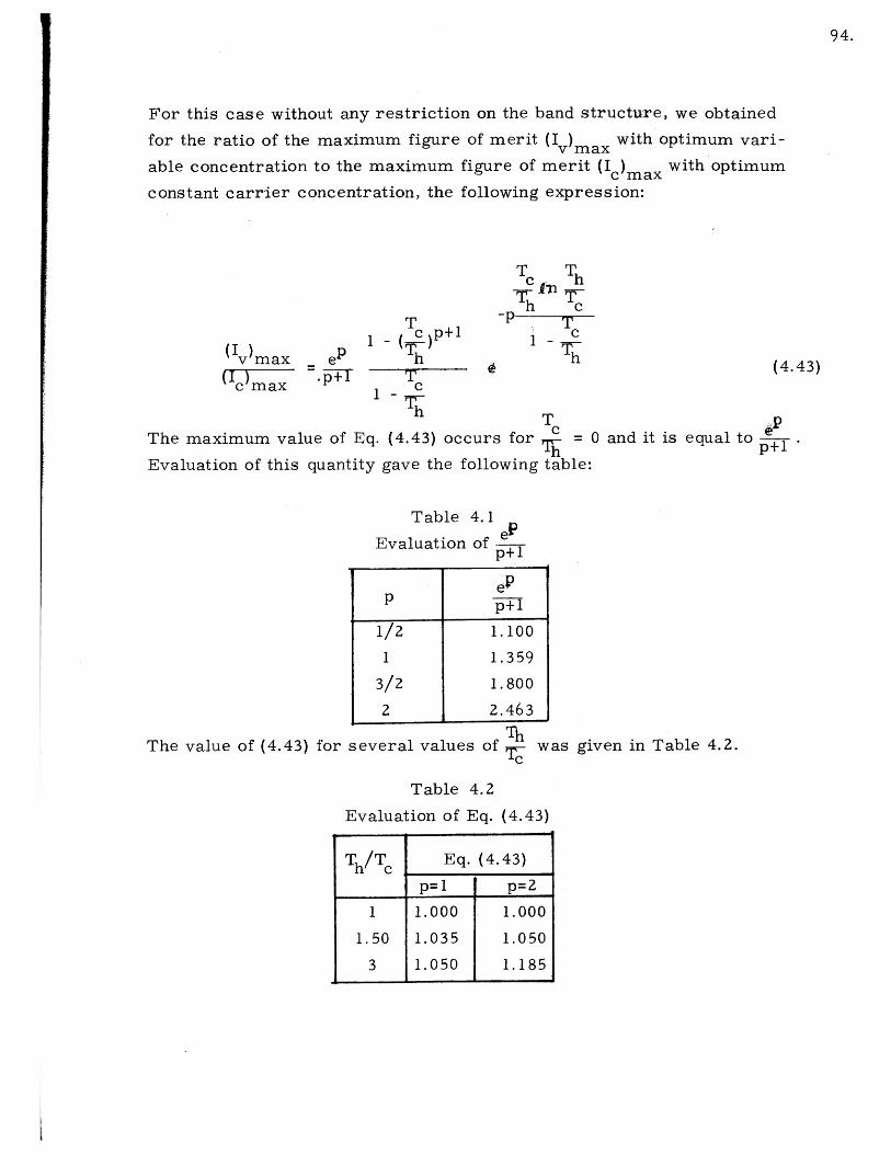
94.

For this case without any restriction on the band structure, we obtained

for the ratio of the maximum figure of merit (IV)max with optimum vari-

able concentration to the maximum figure of merit (I )max with optimum

constant carrier concentration, the following expression:

ep

T1- (c)P+l

ThTc

h

T Tch

h c

c

h

The maximum value of Eq. (4.43) occurs for c

Evaluation of this quantity gave the following tab

Table 4.1

Evaluation of e

p+p

p p+11/2 1.100

1 1.359

3/2 1.800

2 2.463

The value of (4.43) for several values of was

= 0 and it is equal to

Le:

given in Table 4.2.

Table 4.2

Evaluation of Eq. (4.43)

Th /Tc Eq. (4.43)

p=1 p=2

1 1.000 1.000

1.50 1.035 1.050

3 1.050 1.185

(Iv)v max

c max(4.43)

p+1

1-1-1- Mi

=1 -_____________ __________________

95.

The conclusion drawn from Tables 4.1 and 4.2 is that there is no es -

sential gain in the figure of merit by the use of variable carrier con-

centration except for the case of a strong dependence of the ratio KLupon temperature and for the case of a large ratio of Th to T

6.2 Conclusions from the Experimental Results

First we shall state the conclusions about the properties of p+type

and n-type cast lead telluride deduced from the measurements performed

on the material:

a. The Lorentz number for p and n type material was found

to be 1.73 from thermal conductivity measurements (Fig.

5.10). Considering possible experimental errors, it was

concluded that the scattering in the material is predom-

inantly atomic scattering.

b. The thermoelectric power of p-type material had a larger

rate of increase with respect to temperature than did the

n-type material (Figs. (5.4) and (5.5)). Assuming classical

semiconductor theory, a plausible explanation was that the

effective mass had a stronger temperature dependence in

the p-type material than in the n-type material.

c. The temperature dependence of the electric conductivity

upon temperature for the less degenerate p and n-type

material was found to be T~ for the p-type material and-2 5

T 'for the n-type material (Figs. (5.6) and (5.7)). Al-

though we did not have Hall data for the material to deter -

mine the temperature dependence of the mobility, we ob-

tained an estimate of the temperature variation of the ef-

fective mass assuming atomic scattering and constant

carrier concentration. With these assumptions, we con-

cluded that the temperature variations of the effective

masses were:

(m*)p oC T (m*) nC T0 .4 (5.3)

96.

This result is in qualitative agreement with (b).

d. The temperature dependence of the lattice thermal

conductivity was found to follow very closely the law

1/T for both p and n-type material (Fig. (5.13). Next,

we gAve in Table (5.1) the results obtained for the op-

timum constant carrier concentrations and the maxi-

mum figures of merit obtained from Eqs. (4.21) and

(4.23), and from the experimental data Figs. (5.14),

(5.15), and Fig. (5.20):

Table 5.1

Optimization of n and p-type materials

Theory Experiment Error %c n 1650 1250 +32%

op -(0-cm) p 2650 2700 -1.8%

I x n 1.63x10 3 1.96 x 10 3 -16%max3 3

(OK) -__ p 2.16x10 2.01 x 10- +7.5%

*Measured at 300 K.

As additional data to Table 5.1, the actual figure of merit for the n-type

material with a conductivity of 1650 (Q7e-cm) was 1.84 x 10-3 (ck) as ob-

tained from Fig. (5.20). Similarly for the p-type the figure of merit for

a conductivity of 2650 (0-cm)-I was 1.98 x 10 3 ( K) . In Table (5.2)

we gave the results for the optimum constant carrier concentrations for

simultaneous optimization of the n and p-type materials obtained from

Eqs. (4.54) and Fig. (5.19), and from the experimental data obtained by

assuming that optimum constant carrier concentrations are the same as

the carrier concentrations given in Table 5.2.

Table 5.2Simultaneous optimization of the n and p-type materials

Theory Experiment Error%*

n 1800 1250 +43%op -1

(0-cm) p 2500 2700 -7.3%

Ima 1.90x10 1.98x10 -4%

(OK) - a-

* Measured at 300 0K

I -- ' 0 Eh 0 -- ft 1, - --

97.

-1The actual figure of merit obtained using un = 1800(02-cm) and

-1 -3a- = 2500(0-cm) is 1.83 x 10 as determined from Eq. (2.40) andp

Figs. (5.14), (5.15), and (5.19).

Let us consider next the results for the optimum variable carrier

concentration for the p-type material. The ratio between the maximum

figure of merit obtained by using variable carrier concentration to the

maximum figure of merit with optimum constant carrier concentration

from Eqs. (4.23) and (4.37) was found to be:

(I)v max = 1.04c max

The actual figure of merit obtained with variable carrier concentration

according to Eq. (4.33) was found to be:

(I)actual = 2.16 x 10 -3 o )1

This last value should be compared with the value of the actual figure of

merit obtained with constant carrier concentration given in Table 5.1.

(Ic max actual = 2.01 x 10 3 oK)

The improvement in the figure of merit was found to be:

(I)Vactual = 1.08c max actual

Having summarized the numerical results from the theory and the re -

sults from the experimental data, the following general conclusions can

be drawn:

I. From Table 5.1 (Theoretical values from Eqs. (4.21) and (4.33) ex-

perimental values from Fig. 5.20)

la. For materials whose thermoelectric power has a temperature

dependence of the type 3( k) in T, the values for the optimumq

carrier concentration and for the maximum figure of merit

98.

given by the theory are within 10% of the values given

by the experimental data.

2a. For materials whose thermoelectric power has a tem-

perature dependence of the type 2( ) YnT, the value for theqoptimum carrier concentration given by the theory is within

40% of the experimental value, and the value for the maxi-

mum figure of merit given by the theory is within 20% of

the experimental value.

3a. If the theoretical constant carrier concentrations are used,

the experimental figures of merit obtained with them are

within less than 10% of the maximum experimental figures

of merit.

II. From Table 5.2 (Theoretical values from Eqs. (4.54) and (4.50) ex-

perimental values from Fig. 5.20)

2a. In the case of simultaneous optimization of both materials,

the carrier concentrations given by the theory may have an

error as large as 50% with respect to the experimental ones,

but the figure of merit given by the theory is within 10% of

the experimental one.

2b. If in the case of simultan-ous optimization of both materials,

the carrier concentrations given by the theory are used, thewItkn

experimental figure of merit obtained with them isAl0% of

the maximum experimental one.

III. From the results of the optimum variable carrier concentration

(Theoretical values from Eqs. (4.21), (4.23), (4.33), (4.26) and Fig. (5.21))

Experimental values from Figs. (5.21) and (5.22)

3a. The theoretical gain in the figure of merit obtained with the

use of the theoretical variable carrier concentration is within

5% of the experimental gain obtained using the theoretical vari-

able carrier concentration.

99.

From (3a) and (2b) we conclude that, although the theoretical carrier

concentrations may be in large error, the experimental figures of

merit obtained with them differ at most by 10% from the maximum

experimental figures of merit. Therefore, this theory is useful for

determining optimum carrier concentrations.

6.3 Suggestions for Further Work

In conducting the experimental program, some problems were not

investigated because of a lack of time or because they did not have a

close relation to our work. Since the solution to these problems is im-

portant in the field of applied thermoelectricity, the following suggestions

for future studies are made:

a. To develop a method for the direct measurement of the

average values of the parameters. An apparatus similar

to the one used in thermal conductivity measurements may

be adequate. (Fig. 5.3).

b. To perform more experiments in order to determine if the

difference in the thermal conductitrity of the n-type and

p-type lead telluride is caused by the difference in their

composition.

c. To make a careful study of the age-hardening time as 6afunc -

tion of annealing temperature needed to improve the mech-

anical properties of the p-type cast lead telluride.

d. To determine if the mechanical properties of the p-type

cast lead telluride are improved by the addition of tel-

lurium to the highly doped material.

100.

BIBLIOGRAPHY

1. Telkes, M., The Efficiency of Thermoelectric Generators I, Journalof App. Phys., 18, 1116, (1947).

2. Ioffe, A. F., Semiconductor Thermoelements and ThermoelectricCooling (Infosearch Ltd. London), 1957.

3. Borrego, J. M., Lyden, H. A., Blair, J., The Efficiency of Thermo-electric Generators, WADC Technical Note 58-200, Project 6058,M. I. T., DSR 7672, September, 1958.

4. Sherman, B., Heikes, R. R., Ure, R. W., Jr., Computation of Effi-ciency of Thermoelectric Devices, Scientific Paper 431FD410-P3,Westinghouse Research Laboratories, March, 1959.

5. Chasmar, R. P., Stratton, R., The Thermoelectric Figure of Meritand its Relation to Thermoelectric Generators, Journal of Elec. andContr.,7, 52 (1959).

6. Moizhes, B. Ya., The Influence of the Temperature Dependence ofPhysical Parameters on the Efficiency of Thermoelectric Generatorsand Refrigerators, Soviet Physics-Solid State, 4, 671, (1960).

7. Fritts, R. W., Lead Telluride Alloys and Junctions, (ThermoelectricMaterials and Devices, Edited by I. B. Cadoff and E. Miller, ReinholdPublishing Co., New York) 1960.

8. Brebrick, R. F., Allgier, R. S., Composition Limits of Stability ofPbTe, Journal of Chem. Phys., 32, 1826 (1960).

9. Wedlock, B., Measurement of Electrical Conductivity at ElevatedTemperatures, Theoretical and Experimental Research in Thermo-electricity, M. I. T. Energy Conversion Group, Scientific Report no. 1Contract AF19(604)-4153, December, 1959.

10. Lyden, H. A., High Temperature Thermal Conductivity and SeebeckCoefficient Measurements, Theoretical and Experimental Researchin Thermoelectricity, M. I. T., Energy Conversion Group, ScientificReport No. 1, Contract AF19(604)-4153, December, 1959.

11. Gershtein, E. Z, Stavitskaia, T. S., Stil' bans, L. S., A Study of theThermoelectric Properties of Lead Telluride, Sov. Phys., Tech.Phys, 2, 2302, (1951).

12. Deviatkova, E. D., A Study of the Thermal Conductivity of Lead Tel-luride, Sov. Phys., Tech. Phys, 2, 414, (1957).

13. Kanaii, Y, Nii, R., Experimental Studies on the Thermal Conductivityin Semiconductors, Phys. and Chem. of Solids, 8, 338, (1958).

101.

APPENDIX A

Optimum Carrier Concentration for Maximizing the

Product of the Figure of Merit and the Average

Temperature: Derivation of Equations

Appendix A derives the equations to be satisfied by the optimum

constant and variable carrier concentrations in order to maximize the

product I of Eqs. (2.20) and (2.21). Multiplication of the above equa-

tions gives:

= 2(fadT)(fTcdT)AT(f pK dT)2

_ (fadT) 2 (fTpKdT)

AT(f p K dT)(A.1)

Consider first the case of constant carrier concentration. Taking

the derivative of (A.1) with respect to n and equating to zero, we obtain:

~f fTdT

-f 2fadT fTadT2

L(fpKdT)

fadT JTpKdT

(fpKdT)2

2(fadT) 2fTpKdT

(fpKdT)

fadT aa dTTfpxdT ai KT

T(fadT) 2 apK dT - 0

(fpKdT) an S=

From the above equation it follows that:

f(1 + ) - - dT - Cf(2+ ) -P' dT = 0

C - 1 fadT2 JpKdT

D fTadTf dT=-

(A.4)

(A.5)fTpKdTfpKdT

Equation (A.3), (A.4) and (A.5) are the necessary conditions for (A.1) to

have a stationary value.

The derivation of the equations for the optimum variable carrier

dT0

dn

(A. 2)

where:

(A.3)

102.

concentration follow the same lines as in Chapter III. The result is anexpression identical to (A.2) but with the function m(T)) Inside of theintegral. Since m(T) is, by hypothesis, arbitrary it follows that:

(+T Ba T &pK+ ) a - C(2+T) n = 0

which can be written:

aa - C(1+D+T n

(A. 6)

(A.7)

Equations (A.4), (A.5) and (A.7) determine the optimum variable carrierconcentration.

103.

APPENDIX B

Optimum Carrier Concentration for Maximizing the

Product of the Figure of Merit and the Average

Temperature: Approximate Solution for a

Non-Degenerate Semiconductor

The equations derived in Appendix A are applied to a non-degenerate

semiconductor with parabolic bands and with no electronic thermal con-

ductivity. We give a first order approximate solution and show that the

solution is very approximate to the Equations of Sec. (4.2).

The material parameters of a non-degenerate semiconductor with

parabolic bands and without electronic thermal conductivity are:

a= (k )[/2+ X +In N](B.1)

KLpKL (B.2)

where:

27r M /(jT 3/2N = 2(- h2 -)'(B.3).

X = scattering parameter.

All the above terms have been defined in Sec. (4.1) .

Let us consider first the case of constant carrier concentration.

Substitution of Eqs. (B.1) and (B.2) into Eq. (A.3) gives:

k )(1 + T) dT + C f(2+ ) L dT = 0 (B.4)

from which we obtain

Th+T (aT)h c _av2 (a)

(a) =2( ) 1 + av (B.5)av q (a T)av (TpK)av

2 av av

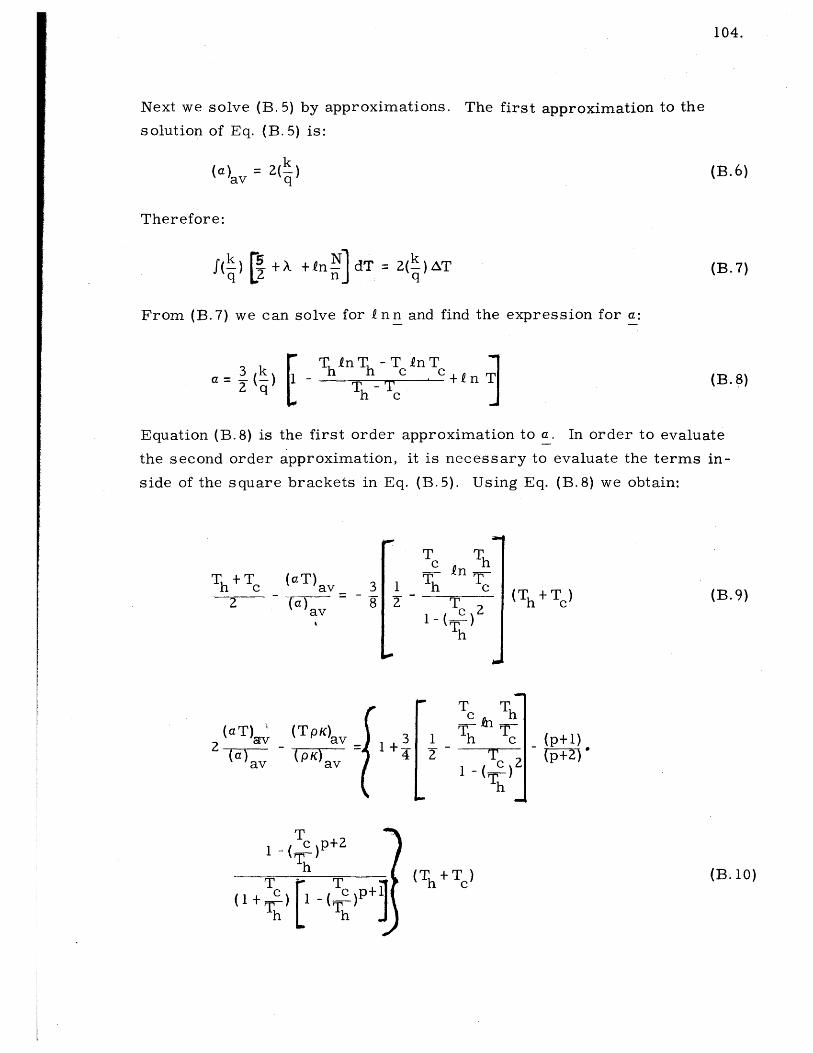
Next we solve (B. 5) by approximations. The first approximation to the

solution of Eq. (B.5) is:

(a)av 2()aveoq

Therefore:

f(k) +X +in dT 2( k)AT

(B.6)

(B.7)

From (B.7) we can solve for Inn and find the expression for a:

3k[ ThinT -T inTThT c+T

(B.8)

Equation (B.8) is the first order approximation to a. In order to evaluate

the second order approximation, it is necessary to evaluate the terms in-

side of the square brackets in Eq. (B.5).

(a T) av

~(a) aav

(T p K)av

av

T1 - p+2

h

Using Eq. (B.8) we obtain:

Tc Th

Th Tc

TS c2

Th

T Tc 1hh

Th Tc

1 -()

(Th + T)

_ (p+1)

(p+ 2 )'

(Th + Tc)

104.

Th+TcTh c

2

(a T)av

av

(B.9)

(1 +

(B. 10)

-U

105.

where we have assumed eKLC TP.

In Table (B. 1) the values are given of the ratio of Eq. (B.9) to Eq.

(B.10) for the case p=2 as n function of Th /Tc

Table B.1

Values of Eq. jB.9)/Eq. (B.10) for p=2

Th Eq. (B.9)

T~ Eq. (B.10)C

1 0

2 -0.028

3 -0.068

From the above values we conclude that the value of (a)av is within 100

of the value given by Eq. (4.12).

Let us consider now the case of variable carrier concentration.

Substitution of Eqs. (B.1) and (B.2) in Eq. (A.7) gives:

pK (-) -____)

PKL~q 1 D+T 2D+T

Equation (B. 11) shows that now PKL is not constant but depends upon T,

however, we will show that this dependence can be neglected. The first

order approximate solution of Eq. (B.11) is:

PKL =( )

(B.11)

(B.12)

Therefore the carrier concentration is of the type BTP if the temperature

dependence of pK L is TP. The carrier concentration BTP is determined

from the condition that:

(a)av = 2( ) (B.13)av q

which is obtained from (B.12). the expression for the first order approxi-

mation in a obtained from Eq. (].13) is:

TkInT -T inT 1k 3 h h c c ~3_a= ( ) 2 - a p) T c v +( -p)fnrT

Using the above value of a_ we obtain the value for D:

D = faTdTD adT

fTpKdTfpKdT

TiTc I

.h + Tc) 1 3 P) Th Tn

21-T

Th

For p = 3/2 the value of D is zero. In this case (B. 13) is the exact solution.

The reason is that the thermoelectric power is independent of tempera-

ture at the optimum variable carrier concentration.

In Table (B.2) the values of the quantity:

D2D+T

at T = T and Tc =Th for the case p=2 as a function of Tc /Th are listed.

Table B.2D

Range of Variation of 2D+T for p=2

D

Th/TC 2D+TTh c

T=T T=Tc h

1 -0.167 -0.167

2 -0.225 -0.107

3 -0.735 -0.122

From the above values we conclude that for Th /Tc < 2 and for p=2 the

solution given by Eq. (B. 11) is very close to the solution given by

Eq. (4.25).

(B.14)

(B.15)

106.

107.

APPENDIX C

Optimum Impurity Distribution for Maximizing the

Figure of Merit: Equations for the Reduced

Fermi Level in a Degenerate Semiconductor

Appendix C derives the equation to be satisfied by the reduced

Fermi level of the optimum variable carrier concentration in a de-

generate semiconductor. The discussion is restricted to the case

of parabolic bands and no electronic component in the thermal con-

ductivity.

The material parameters for a degenerate semiconductor with

parabolic bands are given by:

2n N F 1 /2() (C.1)

( + )Fa= ( )Z F 3 /2 +r (C.2)

q (3) +X)F

3 ( +XA) KLr p+) (C. 3)pKL Npo F1/2+(

where:

p = mobility in the non-degenerate material.

f'(x) = gamma function of x.

Fx(r) = Fermi function = f f(r)deX 1 r

o 1+ exp(e+rj)

Our convention regarding r7 as positive within the gap and negative if

within the band. Properties of the Fermi functions are as follows:

F (ri) = in(l + e) (C.4)

dF( (r5)dr = - X Fx _(r;) (C.5)

JI K b"' -

108.

Equations (C.1), (C.2) and (C.3) indicate that in this case the carrier

concentration A is not a suitable variable to be optimized. The re-

duced Fermi level is a better choice. For the case of the optimum

constant carrier concentration, the optimum reduced Fermi level is

that function of temperature which maximizes the figure of merit

with the additional condition of making Eq. (C. 1) a constant for any

temperature. In the case of the optimum variable carrier concentra-

tion no additional restriction is set on the reduced Fermi level. For

this last case, a similar reasoning as in Sec. 3.2 gives:

a P C K L 0 (C.6)

as the equation to be satisfied by the optimum reduced Fermi level.

Substitution of Eqs. (C.2) and (C.3) in (C.6) give:

k F 5 1/(1 3/2+X FpKL C 1 F L 3X (C. 7)

('+X )F + X) F + X1 _ 12+X L1/2

where use has been made of Eq. (C.5).

It is less important to discuss the solution of Eq. (C.7) than it is to

determine how well the solution given by Eq. (4.25) satisfies Eq. (C.7).

Let us consider the case of atomic scattering, i.e. X = -1/2. For this

case, Eq. (C.7) reduces to:

pKL () 2 F (rj)(1 +e) (C.8)

A plot of the factor in square brackets in Eq. (C. 8) is given in Table C. 1

Table C.1

Value of C(q) p/< from Eq. (C 8)k Ln

2 - F(rj) (1+e")

1 1.003

. 0.5 0.993

0 0.986

-0.5 0.972

-1.0 0.956

109.

The above values show that if the reduced Fermi level is between -1

and 1, the value of pKL is approximately constant.

In Fig. (5.22) the value of the thermoelectric power is plotted for

the optimum variable. carrier concentration given by Eq. (4.25). From

the figure and Eq. (C.2) for X= - 1/2, we find that the reduced Fermi

level is between -1 and 1. Therefore, we conclude that the solution with

Maxwell-Boltzman statistics is very close to the solution with Fermi-

Divac statistics. This is one of the reasons of the close agreement

between Eqs. (5.14) and (5.18).

110

Biographical Note

Jose M. Borrego Larralde was born in 1931 in Ojuela, Durango;

Mexico. He received the Ing. Mecanico-Electricista Degree from the

Institute Tecnologico y de Estudios Superiores de Monterrey in June,

1955. During the year 1955-1956 he came to M.I.T. as a Fullbright

student. In September, 1956, he was appointed Teaching Assistant

in Electrical Engineering at M. I. T. He received the S. M. Degree

in June, 1957 and the E. E. Degree in June, 1958. With a leave of ab-

scence from M. I. T., he spent the last six months of 1958 in Mexico

teaching courses in Electric Machinery. During January, 1959, his

staff rank at M. I. T. was raised to that of Instructor. Since then, he

has been associated with the Energy Conversion Group where he has

been working on thermoelectric device analysis and lately on thermo-

electric materials.

As a staff member, he has taught laboratory courses in energy

conversion and recitation sections on circuit theory and energy con-

version.

He is a member of I. R. E., A. I. E. E., Tau Beta Pi, and Sigma

Xi.

Publications: "Efficiency of Thermoelectric Generators", (co-authors

J. Blair, H. Lyden). W. A. D. C. -Technical Note 58-200,

(1958).