Optimizing the trajectory of a wheel loader working in short loading cycles

R. Filla

Emerging Technologies, Volvo Construction Equipment, Eskilstuna, Sweden E-mail: reno.filla@volvo.com

Abstract A study into alternative trajectories for wheel loaders working in short loading cycles has been conducted, examining other patterns than the traditional V- or Y-cycle. Depending on workplace setup and target function of the optimisation other trajectories can indeed prove beneficial. The results of this study can be used in operator models for offline simulations as well as for operator assistance or even in controllers for autonomous machines or energy management systems for non-conventional machines like hybrids.

Keywords: wheel loader, working cycle, trajectory, work pattern, simulation, operator model, control, operator assistance

1 Introduction Figure 1, published in its first version in [1] and quoted in several publications, shows the classic short loading cycle with the characteristic driving pattern in the shape of a V, possible to extend to a Y, if necessary.

Figure 1: Short loading cycle in classic V- or Y-pattern.

From phase 1 to 6, the wheel loader operator first fills the bucket in the gravel pile, then drives backwards towards the reversing point (phase 4) and steers the wheel loader to accomplish the aforementioned characteristic V-pattern. The lifting function is engaged the whole time. The operator chooses the reversing point such that having arrived at the load receiver and starting to empty the bucket (phase 6), the

lifting height will be sufficient to do so without delay. In case of a bad matching between the machine’s travelling speed and the lifting speed of the bucket, the operator needs to drive back the wheel loader even further than necessary for manoeuvring alone. This additional leg transforms the V-pattern into a Y-pattern.

In the remaining phases 7 to 10, the bucket needs to be lowered and the operator steers the wheel loader back to the initial position in order to fill the bucket again in the next cycle.

While the different phases of the depicted loading cycle are generally applicable (even though in other circumstances it might be meaningful to introduce new phases and events or combine some of the phases shown in Figure 1), the driving pattern does not necessarily have to resemble a V or Y. It appears that this pattern has emerged from the operators’ desire to minimise the personal workload, rather than maximise energy efficiency, for a required productivity.

For new non-conventional systems like (semi)autonomous machines or hybrids, where the operator’s requirements are less dominant or taken out of the loop completely, the traditional cycle in Figure 1 is not necessarily the most productive or the most energy-efficient way, either. Improved energy management for such machines may involve some kind of optimal control scheme along a pre-defined trajectory – so the obvious question would be whether there is optimisation potential in the trajectory itself.

Even if accepting the V/Y-cycle as the trajectory to use, it is an interesting question how to best orient the load receiver for a given position. The traditional recommendations are a 90° or 135° angle, given not only by Volvo but also other players in the industry [2][3]. However, also these recom-mendations are based on the performance of conventional

307

The 13th Scandinavian International Conference on Fluid Power, SICFP2013, June 3-5, 2013, Linköping, Sweden

systems and might not be valid for autonomous machines or hybrids.

There is therefore a need to examine this in more detail and the results can have various applications, from improved dynamic simulations by adding planning capabilities to operator models [4] over off-line use for education or site planning purposes [5][6], on-line operator assistance functions [7] to autonomous machines [8] and improved energy management in advanced systems [9][10][11][12].

2 Problems of the classic V-/Y-cycle A first attempt at examining different driving patterns has been made by the author in [4] – however the work then focused on a specific variant of the classic V-cycle without further consideration of alternatives. When using this trajectory in various workplace setups it becomes apparent that its use is limited to tight places with loading and unloading spot in close vicinity. For larger distances and other orientations of the load receiver, the classic V-cycle with equal steering to both sides very quickly results in unreasonable long transporting distances (Figure 2 left and right).

Figure 2: Classic V-cycle for different locations of the load receiver (left) and different orientations (right).

This stems from the cycle being modelled as simply two circular arcs meeting tangential in the reversal point. For larger workplaces an experienced operator would gradually vary the curve radius or at the very least extend the classic trajectory with line segments rather than travel such long distances in a curve with a very large radius.

Furthermore, above a certain transport distance any operator will start using the wheel loader in a Load & Carry cycle instead (Figure 3). In the “grey” area between tight working places and wide ones other shapes of loading cycle trajectories can serve as a smooth transition. Several possible candidates have been examined in this study; equations have been derived for easy implementation both on-line and off-line.

Figure 3: Load & Carry cycle.

3 Overview of examined cycle variants Expanding upon the variants briefly touched upon in [4] Figure 4 shows the main cycle types and their respective sub-variants that have been examined in this study.

Figure 4: Main cycle types and sub-variants examined in this study. (Depicted load receiver position and orientation

is just an example.)

10− 0 10 20

60−

40−

20−

0

10− 0 10 20

60−

40−

20−

0generic (g) compact (c)

(min #sections)extreme (x)(min turn radius)

A

B

C

D

E

F

G

Sub-variant

Mai

n ty

pe

H

I

(classic)

(same as Cc)

(same as Cc)

308

The first five main types “A” to “E” constitute a systematic exploration of the classic V-/Y-cycle (which is labelled “C”), while “F” and “G” represent a more intricate type with one S-shaped leg and the other one straight. Finally, “H” and “I” are permutations of the “C”-type with reversed order of line and arc section in the second leg (“H”-type), and first leg (“I”-type), respectively.

All cycles types studied can actually be seen as special cases of one unified cycle type with the following properties:

• S-shaped legs with a linear section in between the arc segments

• Length of linear segments can vary in interval (-∞, ∞)

• Radius of arc segments can vary in interval {[-∞, -Rmin_turn) , [Rmin_turn, ∞]}

• Section angle of arc segments can vary in interval [0, 360°)

However, this unified cycle would have seven degrees of freedom and an extremely large search space, due to the parameter intervals also covering negative values. With the current approach and the current tools at hand this seems infeasible to solve in a reasonable amount of time.

Apart from the generic variant (sub-labelled “g”) with the highest amount of degrees of freedom, each cycle type can also be realised either as a compact cycle (sub-labelled “c”) with as few segments per leg as possible or as an extreme variant (“x”) where all curves are executed with highest articulation angle and therefore smallest possible turning radius.

4 Analysis Table 1 shows the amount of degrees of freedom for each cycle variant. While for example “Bc”, the compact variant of the “B”-type, is fully constrained by the three parameters of the workplace setup: orientation of the load receiver and its vertical and horizontal distance from the loading spot, the “Cg” variant has three degrees of freedom left to constrain, which means that a parameter optimisation needs to be performed, for example varying the angle of reversing and the turning radii of both legs.

The equations for all cycle variants have been derived analytically in order to achieve fast calculation. They have been implemented in a collection of MathCad worksheets and verified with parametric profiles in SolidEdge.

The high amount of degrees of freedom for certain cycle variants and thus the necessity of parameter optimisation has an impact on calculation times, however. Even though each individual cycle variant can be calculated fairly quickly, finding the optimal cycle with an optimal load receiver orientation (i.e. an additional degree of freedom) for a given load receiver position takes some seconds nonetheless. Performing a massive workplace sweep as in Figure 15 and Figure 16 takes several days on an average PC.

Table 1: Degrees of freedom for each cycle variant.

All cycle variants can be calculated in “strict” and “non-strict” mode. In the former, the wheel loader is forced to always arrive perpendicular to the load receiver, i.e. in a 90° angle. An example from the field for such a scenario is an immobile crusher with a ramp: neither can the crusher be moved or rotated, nor can the wheel loader enter the ramp other than reasonably aligned.

In contrast to this a conveyor belt, a pit or a submerged truck are all fixed in position and orientation, but the wheel loader serving them has some freedom in the approach for un-loading. In “non-strict” calculations a permitted interval for the angle of arrival is introduced, which adds an additional degree of freedom and therefore increases calculation time even more.

4.1 Delimitations

We only consider the part of the cycle between bucket filling and bucket emptying, i.e. phases 2-5 according to Figure 1.

The intended use of the results of this study for, among others, on-line operator assistance functions, autonomous machines, and improved energy management in advanced systems excludes the possibility to perform detailed dynamic simulations due to a limited time budget. The focus has therefore been on calculations by means of explicit equations for the trajectory parameters and properties.

However, this has the consequence that the effects of the intricate dynamical interaction of engine, drive train and hydraulics cannot be studied. One result is that all curve trajectories are simplified as circular arcs. While circular arcs merging tangential into each other seems smooth to the outside observer, for the wheel loader it is not a smooth manoeuvre at all. Any sudden change of curve radius requires an equally sudden change of articulation angle. With the masses of front and rear frame of a wheel loader, this not only requires a certain amount of energy, but also produces violent jerking. The use of arcs with a constant radius is therefore only correct for a constant articulation angle (Figure 5).

Sub-variant

g c x

A 2 1 0

B 1 0 0

C 3 1 1

D 1 0 0

E 2 1 0

F 3 2 1

G 3 2 1

H 3 (1) 1

I 3 (1) 1

Mai

n ty

pes

309

Figure 5: Wheel loader in a turn, fixed articulation.

Any path transition needs to employ smooth changes of radii. In most situations the wheel loader will be in longitudinal motion while the steering function is used to slowly change the frame articulation from a start value to a value that results in the required turning radius (Figure 6)

Figure 6: Wheel loader in a turn, several stages from straight to full turn.

This means that instead of following an arc with a constant radius the wheel loader’s track will rather resemble a clothoid or Euler spiral (provided that the change in articulation angle is linear). Figure 7 shows in top view how the curvature of a wheel loader’s trajectory is affected by different machine speeds: in all traces (simulating a L120G wheel loader model for 20s) the steering angle is increased with a steering speed of 20% of maximum possible, beginning with a straight machine (0° articulation) and a cut-off at the machine’s maximum articulation angle. The dashed line represents the theoretical turning circle, which assumes an already established articulation angle of maximum value. It can be seen that the higher the machine speed, the higher the deviation of the actual trajectory from the theoretical turning circle.

Figure 7: Wheel loader trajectories for different machine speeds at constant steering speed (linearly increasing

articulation from 0° with cut-off at maximum).

Figure 8 shows how the curvature of a trajectory is affected by different steering speeds (again simulating a L120G wheel loader model for 20s). Not surprisingly, the lower the steering speed, the higher the deviation of the actual trajectory from the theoretical turning circle.

Figure 8: Wheel loader trajectories for different steering speeds (linearly increasing articulation from 0° with cut-off

at maximum) at constant machine speed.

Modelling the curve trajectories as clothoids would require a detailed simulation model that provides correct values for machine speed and steering angle over time, which in turn requires detailed modelling of the complete machine system including actuation by the operator, engine dynamics, and how hydraulics and drive train compete for the limited engine power available.

As mentioned before, several of the intended applications of the results of this study do not allow any detailed simulation to be used anyway. In the case of optimal control we also have arrived at a Catch-22 situation, where we would need a detailed simulation in order to optimally control for example energy management of a hybrid machine – in a simulation.

0 10 20

0

10

20

2.5 km/h, steeringspd 20%5 km/h, steeringspd 20%10 km/h, steeringspd 20%theor. turning circle

0 10 20

0

10

20

5 km/h, steeringspd 100%5 km/h, steeringspd 20%5 km/h, steeringspd 10%theor. turning circle

310

For this study we have therefore chosen to simplify and approximate curves as circular arcs nonetheless. This enables an analytical solution to all cycle variants to be examined, which has a beneficial effect on the calculation time that is required for optimisation.

This simplification leads to quite a significant deviation of the actual machine position from the theoretical turning radius when an established and maintained machine speed of typically 10km/h is considered (Figure 9).

Figure 9: Error in position calculation due to simplification (circular arcs instead of clothoids)

However, if we assume that for the most part a steering action coincides with an acceleration of the machine from stand-still (probably never attaining the typical speed of 10km/h), then the error caused by the simplification of clothoid segments to circular arcs is tolerable, especially for target steering angles of 20° and below (Figure 10).

Figure 10: Error in position calculation due to simplification (circular arcs instead of clothoids)

4.2 Boundary conditions

The equations for cycle variant are set up so that the wheel loader trajectory always joins perpendicular to the loading spot and load receiver. The non-strict calculation mode, in which the machine’s angle of arrival at the load receiver is allowed within a pre-specified interval, is realised by varying the load receiver orientation within the same interval and perform strict calculations.

The arc segments have to be executed with a radius at least equal to the specified wheel loader model’s minimum turning radius.

Line segments that are enclosed by arcs and connect to the reversing point are allowed to have negative length, so that they can be executed either before or after reversing. This applies to variants of cycle types “A”, “E”, “H” and “I”.

Additional boundary conditions ensure that prohibited territory is not violated. For example, the trajectory is only allowed to approach both load receiver and loading spot from the front. It may also not go behind either one. The left image in Figure 11 shows all such invalid trajectories (in grey) for cycle variant “Cg” in a specific workplace setup. The red trajectory is the optimal one.

Figure 11: Examples of valid and invalid trajectories

A safety perimeter (dotted circle in Figure 11) is established around the load receiver, ensuring that trajectories do not collide with the dump truck or crusher placed there. The right image in Figure 11 shows all such invalid trajectories (in grey) for cycle variant “Ec” in a specific workplace setup. In the calculations performed in this study the safety radius has been set to 3 meters.

4.3 Optimisation of cycle parameters

The degrees of freedom shown in Table 1 for each cycle variant mean that the cycle trajectory is not fully constrained just by knowing the load receiver position and orientation (as discussed previously, these can become additional degrees of freedom). Instead, some cycle parameters need to be set explicitly – not by chance with a random value but through optimisation with a value that maximises or minimises a chosen property of the cycle.

Since most (if not all) optimisation problem in this study are ill-conditioned and also non-smooth due to the boundary conditions, after initial trial runs with different optimisation algorithms it was decided to implement brute force opti-misation instead. In most cases the optimisation parameter was an angle that was to be varied in an interval of 180° or less. Sweeping this interval in steps of one degree was easy to do and improved performance noticeably. It was reasoned that this would be precise enough because a human operator is hardly able to perform a turn with even this precision.

But which target function to use for optimisation, i.e. what distinguishes a better cycle in comparison to another variant? The properties listed below are good candidates:

4− 2− 0 2 4

0

2

4

6

Position error in (x, y)

Δx (m)

Δ y (m

)

0 5 10 15 200

2

4

6steer to 10°steer to 20°steer to 30°steer to 40°

Total position error over time

time (s)

Δ (m)

4− 2− 0 2 4

0

2

4

6

Position error in (x, y)

Δx (m)

Δ y (m

)

0 5 10 15 200

2

4

6steer to 10°steer to 20°steer to 30°steer to 40°

Total position error over time

time (s)

Δ (m)

311

1. driving distance 2. driving time 3. driving time including time for steering 4. productivity 5. energy efficiency 6. operator workload

We will discuss these proposals in the following sections.

4.4 Optimisation for driving distance

This is the most simple target function as it involves only the calculation of the length of each individual segment, which has to be done anyway.

It can be argued that optimising for “driving distance” also covers the fuel consumption caused by energy requirements of the drive train – at least to a certain extent, though not in any greater detail.

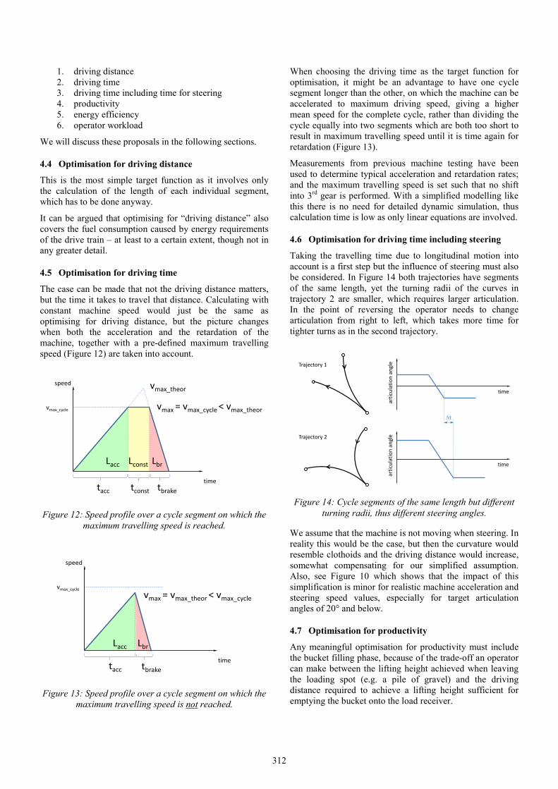
4.5 Optimisation for driving time

The case can be made that not the driving distance matters, but the time it takes to travel that distance. Calculating with constant machine speed would just be the same as optimising for driving distance, but the picture changes when both the acceleration and the retardation of the machine, together with a pre-defined maximum travelling speed (Figure 12) are taken into account.

Figure 12: Speed profile over a cycle segment on which the maximum travelling speed is reached.

Figure 13: Speed profile over a cycle segment on which the maximum travelling speed is not reached.

When choosing the driving time as the target function for optimisation, it might be an advantage to have one cycle segment longer than the other, on which the machine can be accelerated to maximum driving speed, giving a higher mean speed for the complete cycle, rather than dividing the cycle equally into two segments which are both too short to result in maximum travelling speed until it is time again for retardation (Figure 13).

Measurements from previous machine testing have been used to determine typical acceleration and retardation rates; and the maximum travelling speed is set such that no shift into 3rd gear is performed. With a simplified modelling like this there is no need for detailed dynamic simulation, thus calculation time is low as only linear equations are involved.

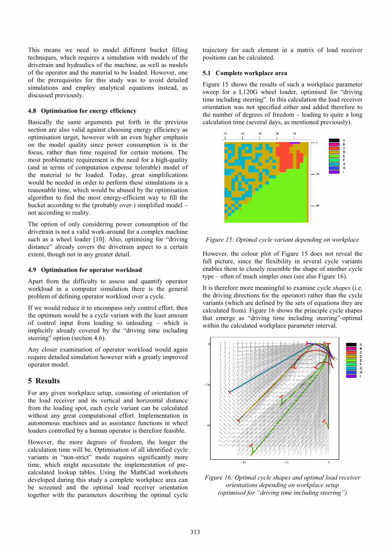
4.6 Optimisation for driving time including steering

Taking the travelling time due to longitudinal motion into account is a first step but the influence of steering must also be considered. In Figure 14 both trajectories have segments of the same length, yet the turning radii of the curves in trajectory 2 are smaller, which requires larger articulation. In the point of reversing the operator needs to change articulation from right to left, which takes more time for tighter turns as in the second trajectory.

Figure 14: Cycle segments of the same length but different turning radii, thus different steering angles.

We assume that the machine is not moving when steering. In reality this would be the case, but then the curvature would resemble clothoids and the driving distance would increase, somewhat compensating for our simplified assumption. Also, see Figure 10 which shows that the impact of this simplification is minor for realistic machine acceleration and steering speed values, especially for target articulation angles of 20° and below.

4.7 Optimisation for productivity

Any meaningful optimisation for productivity must include the bucket filling phase, because of the trade-off an operator can make between the lifting height achieved when leaving the loading spot (e.g. a pile of gravel) and the driving distance required to achieve a lifting height sufficient for emptying the bucket onto the load receiver.

vmax_theor

vmax = vmax_cycle < vmax_theor

time

speed

tacc tconst tbrake

vmax_cycle

Lacc Lconst Lbr

vmax = vmax_theor < vmax_cycle

time

speed

tacc tbrake

vmax_cycle

Lacc Lbr

Trajectory 1

Trajectory 2

timear

ticul

atio

nan

gle

time

artic

ulat

ion

angl

e

∆t

312

This means we need to model different bucket filling techniques, which requires a simulation with models of the drivetrain and hydraulics of the machine, as well as models of the operator and the material to be loaded. However, one of the prerequisites for this study was to avoid detailed simulations and employ analytical equations instead, as discussed previously.

4.8 Optimisation for energy efficiency

Basically the same arguments put forth in the previous section are also valid against choosing energy efficiency as optimisation target, however with an even higher emphasis on the model quality since power consumption is in the focus, rather than time required for certain motions. The most problematic requirement is the need for a high-quality (and in terms of computation expense tolerable) model of the material to be loaded. Today, great simplifications would be needed in order to perform these simulations in a reasonable time, which would be abused by the optimisation algorithm to find the most energy-efficient way to fill the bucket according to the (probably over-) simplified model – not according to reality.

The option of only considering power consumption of the drivetrain is not a valid work-around for a complex machine such as a wheel loader [10]. Also, optimising for “driving distance” already covers the drivetrain aspect to a certain extent, though not in any greater detail.

4.9 Optimisation for operator workload

Apart from the difficulty to assess and quantify operator workload in a computer simulation there is the general problem of defining operator workload over a cycle.

If we would reduce it to encompass only control effort, then the optimum would be a cycle variant with the least amount of control input from loading to unloading – which is implicitly already covered by the “driving time including steering” option (section 4.6).

Any closer examination of operator workload would again require detailed simulation however with a greatly improved operator model.

5 Results For any given workplace setup, consisting of orientation of the load receiver and its vertical and horizontal distance from the loading spot, each cycle variant can be calculated without any great computational effort. Implementation in autonomous machines and as assistance functions in wheel loaders controlled by a human operator is therefore feasible.

However, the more degrees of freedom, the longer the calculation time will be. Optimisation of all identified cycle variants in “non-strict” mode requires significantly more time, which might necessitate the implementation of pre-calculated lookup tables. Using the MathCad worksheets developed during this study a complete workplace area can be screened and the optimal load receiver orientation together with the parameters describing the optimal cycle

trajectory for each element in a matrix of load receiver positions can be calculated.

5.1 Complete workplace area

Figure 15 shows the results of such a workplace parameter sweep for a L120G wheel loader, optimised for “driving time including steering”. In this calculation the load receiver orientation was not specified either and added therefore to the number of degrees of freedom – leading to quite a long calculation time (several days, as mentioned previously).

Figure 15: Optimal cycle variant depending on workplace

However, the colour plot of Figure 15 does not reveal the full picture, since the flexibility in several cycle variants enables them to closely resemble the shape of another cycle type – often of much simpler ones (see also Figure 16).

It is therefore more meaningful to examine cycle shapes (i.e. the driving directions for the operator) rather than the cycle variants (which are defined by the sets of equations they are calculated from). Figure 16 shows the principle cycle shapes that emerge as “driving time including steering”-optimal within the calculated workplace parameter interval.

Figure 16: Optimal cycle shapes and optimal load receiver orientations depending on workplace setup

(optimised for “driving time including steering”)

313

Judging from Figure 16 it seems clear that in the lower right half of the workplace it is better to drive in reverse for most of the distance. This is confirmed by plotting the relative performance of single cycle types such as in Figure 17. It can be seen that cycle type “C” is optimal (or very close to) in the entire upper left area of the workplace, but not so in the lower right area where “E” is optimal (except on the very right edge where “E” is restricted by the safety radius around the load receiver, leaving the field open to “C”).

Figure 17: Relative performance of cycle type “C” compared to optimum in each single location

(optimised for “driving time including steering”)

Figure 17 also reveals that even though cycles types “D” and “G” were presented as optimal in the upper left area of Figure 15, cycle type “C” is more or less equally good. This is again due to the actual shape of cycle types “G” and “C” being optimised to resemble “D” – a sign that the additional degrees of freedom in these cycles are not always needed. However, Figure 18 shows that the area where cycle type “D” is the optimum is not as large as for “C”.

Figure 18: Relative performance of cycle type “D” compared to optimum in each single location

(optimised for “driving time including steering”)

Using such plots it can be shown that cycle type “E” is far from being optimal in the upper left area of the workplace, as well as that cycle types “A” and “B” are inferior in

generally all situations, provided the orientation of the load receiver is not fixed.

However, it is difficult to generalise, since the observations made above are valid for a specific wheel loader model and a specific situation (safety radius, variable load receiver orientation, etc.). In another setup with perhaps a more restrictive safety perimeter around the load receiver and a fixed orientation of the latter it might very well be the case that cycles type “A” is superior to all others.

5.2 Specific load receiver locations, strict

In order to not use overly academic examples we designed a test case that followed the recommendations given in the literature. Acting upon the advice in [2][3] and others that a tight “C”-type cycle shall be driven with no more than 1.5 wheel revolutions per leg or better ¾ to 1¼ (as experienced professionals do), the load receiver, angled at 135° as recommended, was positioned 3m to the side at 2m distance from the loading spot.

Due to the tight work place setup some cycle variants are prevented from reaching a valid solution. Figure 19 shows that no valid solutions could be found for cycle types “E” and “F” when optimising for driving distance. The optimal cycle in this setup is a “C”-type cycle optimised as variant “Cx” (trajectory and bar in red colour in Figure 19).

Figure 19: Test case optimised for driving distance

The blue trajectory and bar in Figure 19 belongs to “CcSR”, a special case of a “Cc” cycle with a boundary condition that both arcs shall have the same radius. This gives the same articulation angle right and left for the wheel loaders operator to steer to – probably a workload-minimising way an operator might want to choose. It is presumed that this (or the rather similar “CcSA”) is close to the classic V/Y-cycle as depicted in Figure 1, where both legs are clearly noticeable arcs (whereas a common “Cc” variant has one degree of freedom left and can be optimised into having the radius of one leg as nearly infinite, thus approaching a straight line).

Driving a cycle according to this classic case “CcSR” would have increased driving distance by 70% compared to the optimal solution (blue trajectory and blue bar in Figure 19).

In comparison to the optimum “Cx”, an optimised “Dg” cycle would have increased driving distance by 20%.

Optimising for driving time instead of driving distance does not result in a significantly different outcome. Those cycle variants with degrees of freedom get optimised into

314

basically the same shape. However, it is interesting to note that the advantage of the optimal variant of “Cx” decreases, so that classic case “CcSR” now only features a 30% higher value for the driving time as opposed to a 70% higher driving distance. The difference is due to the wheel loader using the longer legs to accelerate to higher machine speed, which greatly improves the average cycle speed.

The picture changes more significantly when optimising for driving time including steering. Now there is also a penalty on turning radii which require a lot of steering. Figure 20 shows that this favours a “D”-type cycle (but not “Dc” or “Dx”), presumably because this cycle only requires the wheel loader operator to use the steering function one time during reversing. However, the advantage over, for example the classic case “CcSR” is even smaller than previously: the latter only suffers from a 10% increase in driving time when the effects of steering are included.

Figure 20: Test case optimised for driving time including steering

It is interesting to examine how the result changes with different machine parameter values. For example, in the calculation to the results in Figure 21 the wheel loader’s steering speed has been reduced to half of its original value. This has a profound negative impact on the “x” variants in which all turns are executed with minimum radius, i.e. maximum machine articulation. Cycle “Cx” takes now twice the time to drive compared to the optimised “Dg”. The latter now requires 17.8s to drive, compared to only 11.6s with the original machine.

Figure 21: Test case optimised for driving time including steering, machine with halved steering speed

In Figure 22 the machine performance has been boosted by 100% so that the values for typical acceleration, retardation and steering speed are doubled. This favours a “Cg”-variant that almost resembles the shape of a “D”-type cycle, but not quite (though the driving time including steering is stated as 8.7s in both cases, so the difference is marginal). It is

interesting to see that the relative performance of all cycles now varies less than when calculating with the original machine parameters (Figure 20).

Figure 22: Test case optimised for driving time including steering, machine with doubled acceleration, retardation

and steering speed

5.3 Specific load receiver locations, non-strict

In “non-strict” mode the wheel loader is permitted to arrive at the load receiver with an angular deviation from the exact 90° that the “strict” scenario stipulates.

In the calculations in this study the interval is set to ±15°. Figure 23 shows that this helps cycle type “F” to find a valid solution when optimising for driving distance. The angle deviation utilised by “Fx” is 11°, meaning that the best value of this cycle type is calculated for arrival at 101°. All other cycle types were able to find valid solutions already in “strict” mode and prefer therefore to arrive at 75° instead.

Figure 23: Test case optimised for driving distance, non-strict

In general, Figure 23 shows that “Cx” is still optimal when driving distance is considered – however the classic case “CcSR” now only shows a 50% higher value. It seems that “Cx” profits more from the “non-strict” mode than “Dg”, because the relative performance of the latter is 30% higher than “Cx”, while it was only 20% higher in “strict” mode (for comparison: in “strict” mode the “Cx” cycle resulted in 10.9m driving distance, compared to 9.4m in “non-strict”).

When optimising for driving time including steering, we see that “Dg” is marked as the optimum in Figure 24 (in red), however “Dc”, “Cc” and “Cg” do perform equally well. The conclusion is that in this setup the optimal cycle shape is that of “Dc” and the other cycles resemble that shape in their

315

respective optimised form. The angle deviation utilised is -15°, i.e. the approach angle to the load receiver was 75°.

Figure 24: Test case optimised for driving time including steering, non-strict

In general, “non-strict” calculations will result in less variation in the relative performance of the cycle variants, since each variant competes with many more individuals than in “strict” mode. In the case of “F”-type cycles for our chosen workplace setup we have seen that “non-strict” is required to find a valid solution at all.

5.4 Specific load receiver locations, free orientation

In another set of MathCad worksheets calculations can be performed where the load receiver location is still fixed, but its orientation is considered an additional degree of freedom, also to be optimised. This is in principle a serial execution of the previously described calculations, conducted for all possible load receiver angles in the interval [0°, 180°]. The previously discussed calculation of a complete workplace area is nothing more than a massive application of this, performed for a matrix of load receiver locations.

Also these calculations too can be performed in “strict” or “non-strict” setting, but in order to save space this paper will not feature any example.

6 Discussion The operator model published in [4] can adapt the cycle trajectory to the working place, but the simulated wheel loader will always be made to follow a resembling of the classic “CcSR” case. The example calculations presented in this paper show that this special case is not really optimal in any scenario. The operator model can thus benefit from at least implementing the full “C”-type.

Another application could be optimisation of the layout of a construction site and even education of operators in how to cooperate. Since several cycle types of different shape can turn out to lead to approximately similar results, there might be an opportunity for a sort of traffic management by letting different wheel loaders take different trajectories in order to avoid congestions.

However, it is easy to get carried away by mathematical models, forgetting the delimitations. In this case it is important to remember that in a real wheel loader the

trajectories will be clothoids rather than circular arc, with a curvature that is dependent on the machine speed and the steering speed, which in turn are both dependent on the engine speed, controlled by the operator.

Also the balance of speed of the hydraulic functions and machine speed is important to consider. As discussed earlier, the operator chooses the reversing point such that upon arrival at the load receiver the lifting height will be sufficient to do start emptying the bucket immediately. In case of a bad matching between the machine’s travelling speed and the lifting speed of the bucket, the operator needs to drive back the wheel loader even further than necessary for manoeuvring alone. It is thus not guaranteed that a theoretically optimal cycle variant is actually usable, because the calculations employ static values for important machine parameters such as steering speed and acceleration rate.

It has been discussed in the beginning of this paper that one application could be to give the operator tips in case the machine detects a driving pattern that is perceived to be inefficient. By employing machine learning techniques the limitations of the use of static values may be overcome, at least for a specific machine in a specific application (and perhaps a specific operator, too).

Some, in certain cases slightly better, cycle variants can be hard for a human operator to execute, for example the “E”-type cycle in Figure 16 which involves backing the machine at full speed, passing the load receiver at minimum distance (as prescribed by the safety perimeter, in our examples set to 3m radius). An autonomous machine, on the other hand would have no difficulties at performing this, thus being able to realise even the small improvement potentials that might lie in an optimised cycle pattern.

The example calculations discussed in this report were made for a conventional wheel loader, but there might be a difference for unconventional machines like hydraulic or electric hybrids or a wheel loader equipped with a CVT transmission. In any case energy management in these advanced systems can profit from a higher degree of situation awareness: knowledge about the current working cycle and optimisation possibilities.

7 Conclusions A study into alternative trajectories for short loading cycles of wheel loaders has been conducted, examining other patterns than the traditional V- or Y-cycle. Depending on workplace setup and target function of the optimisation other trajectories can indeed prove beneficial.

The results of this study can be used in operator models for offline simulations as well as for operator assistance or even in controllers for autonomous machines or energy management systems for non-conventional machines like hybrids.

However, the limitations of the approach utilised should be taken into consideration.

316

References [1] R Filla (2003) “Anläggningsmaskiner: Hydraulik-

system i multidomäna miljöer”. Proc. of Hydraulik-dagar 2003, Linköping, Sweden. http://urn.kb.se/resolve?urn=urn:nbn:se:liu:diva-13371

[2] L Stewart (2005) ”Production Heroes: Wheel Loaders. Take-Charge Loader Operators – Fill Trucks Faster”. Construction Equipment, pp 42-46, no. 3, 2005. http://www.constructionequipment.com/take-charge-wheel-loader-operators-fill-trucks-faster

[3] North Pacific Training and Performance, Inc (2008) “Loader Operator Training Manual (Sample Pages) 992G Wheel Loader”. Downloaded 2012-12-15. http://www.north-pacific.ca/LoaderManual-Sample-English.pdf

[4] R Filla (2005) “An Event-driven Operator Model for Dynamic Simulation of Construction Machinery”. Proc. of The Ninth Scandinavian International Conference on Fluid Power, Linköping, Sweden. http://www.arxiv.org/abs/cs.CE/0506033

[5] J Fu (2012) “A Microsopic Simulation Model for Earthmoving Operations”. World Academy of Science, Engineering and Technology, issue 67, pp 218-223. https://www.waset.org/journals/waset/v67/v67-38.pdf

[6] E Uhlin (2012) “Microsimulation of Total Cost of Ownership in Quarries”. Proc. of 17th International Conference of Hong Kong Society for Transportation Studies, Hong Kong.

[7] B Frank, L Skogh, R Filla, A Fröberg, and M Alaküla (2012) “On Increasing Fuel Efficiency by Operator Assistance Systems in a Wheel Loader”. Proc. of International Conference on Advanced Vehicle Technologies and Integration, pp 155-161, ISBN 978-7-111-39909-4, Changchun, China.

[8] J Blom (2010) “Autonomous Hauler Loading”. Master Thesis. Dept. of Innovation, Design and Engineering, Mälardalen University, Västerås, Sweden. http://www.idt.mdh.se/examensarbete/index.php?choice=show&lang=en&id=1019

[9] K Heybroek, G Vael, J-O Palmberg (2012) “Towards Resistance-free Hydraulics in Construction Machinery”. Proc. of 8th International Fluid Power Conference, Dresden, Germany.

[10] R Filla (2009) “Hybrid Power Systems for Construction Machinery: Aspects of System Design and Operability of Wheel Loaders”. Proc. of ASME 2009 International Mechanical Engineering Congress and Exhibition, Vol. 13, pp 611-620. http://dx.doi.org/10.1115/IMECE2009-10458

[11] K Pettersson, K-E Rydberg, P Krus (2011) “Comparative Study of Multiple Mode Power Split Transmissions for Wheel Loaders”. Proc. of The Twelfth Scandinavian International Conference on Fluid Power, Tampere, Finland. http://urn.kb.se/resolve?urn=urn:nbn:se:liu:diva-72630

[12] T Nilsson (2012) “Optimal Engine Operation in a Multi-Mode CVT Wheel Loader”. Licentiate thesis, Linköping University, Linköping, Sweden, 2012. http://urn.kb.se/resolve?urn=urn:nbn:se:liu:diva-80838

317