Optimizing the Open Pit-to-Underground Mining Transition

Barry Kinga, Marcos Goycooleab, A. Newmanc,∗

aColorado School of Mines, Operations Research with Engineering (ORwE) PhD Program, Golden, Colorado, 80401, USAbUniversidad Adolfo Ibanez, School of Business, Penalolen, Santiago, 7941169, Chile

cColorado School of Mines, Mechanical Engineering Department, Golden, Colorado, 80401, USA

Abstract

A large number of metal deposits are initially extracted via surface methods, but then transition under-

ground without necessarily ceasing to operate above ground. Currently, most mine operators schedule the

open pit and underground operations independently and then merge the two, creating a myopic solution. We

present a methodology to maximize the NPV for an entire metal deposit by determining the spatial expanse

and production quantities of both the open pit and underground mines while adhering to operational pro-

duction and processing constraints. By taking advantage of a new linear programming solution algorithm

and using an ad-hoc branch-and-bound scheme, we solve real-world scenarios of our transition model to

near optimality in a few hours, where such scenarios were otherwise completely intractable. The decision of

where and when to transition changes the net present value of the mine by hundreds of millions of dollars.

Keywords: Mining/metals industries: optimal extraction sequence; production scheduling: transition

problem; integer programming applications: exact and heuristic approaches

1. Introduction and Literature Review

The mining industry contributes trillions of dollars annually to the global economy by providing miner-

als, metals, and aggregates. This, and volatile metal prices, make it critical that mines possess an efficient

production schedule, which can be categorized as: (i) short-term (days to months), (ii) long-term (years),

and (iii) strategic (life-of-mine) (Gershon, 1983). A short-term schedule might determine what material to

process on a given day; a long-term schedule may examine production rate changes (Epstein et al., 2014;

Alonso-Ayuso et al., 2015). Finally, a strategic schedule is used to evaluate large capital investments, and

∗Corresponding author: anewman@mines.edu

Preprint submitted to Elsevier July 9, 2016

other decisions that have long-ranging impacts. Because the transition from open pit to underground extrac-

tion affects a mine for the remainder of its operational life, it falls into the category of strategic scheduling.

At the time of this writing, a large number of metal deposits are being extracted via surface methods, but

plan to transition to concurrently or exclusively extracting ore via underground mining methods. For safety

reasons, the underground mine must be sufficiently geographically separated, with horizontally positioned in

situ rock, from the open pit mine via what is typically referred to as a crown pillar. Current industry practice

places the crown pillar based on: (i) largest economically viable open pit mine, or (ii) the extraction method

that results in the largest undiscounted profit for each three-dimensional discretization of the ore body and

surrounding rock. Mine operators tend to delay the transition, leading to NPV losses of up to hundreds of

millions of dollars. We provide a systematic means by which a mine operator can determine the highest

value of a combined open pit and underground design.

The most common method used to extract material is open pit, or surface, mining. Open pit mines vary

in both shape and size, and their design is based on the deposit’s block model, a model which discretizes the

orebody and surrounding rock, and assigns a series of attributes, including mining cost, degree of mineral-

ization (referred to as grade), location, and the cost or profit associated with processing the specific block.

Blocks can be categorized using a minimum cutoff grade; blocks at or above the cutoff grade are sent to the

processing plant, referred to as a mill, while those below the cutoff grade are sent to a waste dump. The slope

angle for the open pit mine, resulting from geotechnical constraints of the host rock, ensures the stability of

the pit’s walls (Crawford and Hustrulid, 1979).

Given the block attributes and slope angle, mine planners determine the largest economically viable

pit for a given deposit, i.e., the ultimate pit limit (Lerchs and Grossman, 1965; Underwood and Tolwinski,

1998). However, while the solution to the ultimate pit limit problem yields the size of the open pit mine,

it provides no indication of the extraction sequence required to maximize its discounted value. Johnson

(1968) originally formulated the open pit block sequencing problem as an integer program that schedules

the extraction of blocks such that the open pit’s value is maximized subject to resource and precedence

constraints.

Solution techniques for open pit block sequencing problems are still widely studied (Ramazan, 2007;

Osanlo et al., 2008; Souza et al., 2010; Topal and Ramazan, 2010; Chicoisne et al., 2012; Shishvan and

2

Sattarvand, 2015). One such recent significant advance for the linear programming relaxation of a general

version of the so-called precedence constrained production scheduling problem (PCPSP), i.e., the open pit

block sequencing problem, is with the use of an algorithm outlined in Bienstock and Zuckerberg (2010),

which exploits the problem structure (Munoz et al., 2015). Lambert et al. (2014) present a guide to formu-

lating and efficiently solving monolithic instances of the open pit block sequencing problem, i.e, without

decomposition.

Underground mining is used when an economically viable deposit is situated sufficiently deep such that

open pit mining is cost prohibitive. There exist many underground mining techniques: (i) open stoping

(Figure 1), (ii) room-and-pillar, (iii) sublevel caving, (iv) drift-and-fill, (v) longwall, and (vi) block caving.

Determining which method(s) to use is typically based on geotechnical constraints, size, and shape of the

deposit (Qinglin et al., 1996). For the purpose of this paper, we confine our discussion to open stoping

mining and its associated sequencing options.

A stope is a large, three-dimensional, mineable volume whose maximum size is correlated with the

geotechnical properties of the host rock, and is the basic unit for stoping methods. The void left by an

extracted stope is sometimes filled with an aggregate to provide structural stability, a process referred to

as backfilling. Most underground stoping mines are separated into vertically spaced levels based on the

maximum stope height, creating a near-regular grid of possible stope positions (Alford, 2006).

Figure 1: (Open Stoping) In this mining method, rib pillars provide stability, as does the backfilling of open voids left by extractedstopes. Stope advance shows the direction in which mining proceeds.

After determining possible locations from which the ore can economically be extracted, i.e., possible

stope locations, mine planners design the development (Alford, 2007; Brazil and Thomas, 2007), which is

required to gain access to the ore, provide haulage routes, and maintain proper ventilation within the under-

ground mine. All stoping activities require the completion of a specific set of development activities before

3

that stope’s extraction can commence. Underground sequencing constraints are created after the design, and

provide rules for the order in which the development and stopes are extracted. Given a fixed design and

sequencing method, we can schedule the underground mining activities to, e.g., maximize NPV, or min-

imize deviation from production targets (Carlyle and Eaves, 2001; Newman and Kuchta, 2007; Martinez

and Newman, 2011; Brickey, 2015; O’Sullivan and Newman, 2015). Trout (1997) provides one of the first

generalized formulations for underground stope scheduling; our formulation is a bit more streamlined than

his in that we do not differentiate between scheduled and actual decisions, and because we assume that once

an activity commences, it must continue at a prescribed rate until finished. The latter characteristic implies

that our model contains no continuous variables. On the other hand, we determine sill pillar placement, i.e.,

locations in which material is left in situ to allow for a change in mining direction, which adds a layer of

complexity.

An early transition model assigns large aggregated blocks to be extracted via open pit or underground

mining methods in order to maximize value of the deposit (Bakhtavar et al., 2008). This idea was later

improved to include the time element and to capture underground capital costs (Newman et al., 2013). In

both previous transition models, there is little differentiation between the mining units used above and below

ground. The mining industry comments on the difficulty of modeling the transition correctly (Finch, 2012);

however, decisions regarding the transition are becoming increasingly relevant (Araneda, 2015). Figure 2

shows an open pit atop an underground mine. The transition zone is depicted as the material that would be

extracted were it done via underground methods; the corresponding amount of material would greater were

open pit methods used in the transition zone.

We present a new model and corresponding solution techniques to determine the timing of a transition

from open pit to underground mining in both a spatial and a temporal sense. This transition incorporates

a crown pillar placement that separates the open pit from the underground mine, and of the sill pillars,

i.e., levels left in situ that can grant earlier access to stopes by creating a false bottom. Our methodology is

based on an ad-hoc branch-and-bound approach that incorporates decomposition methods for solving PCPSP

linear programming relaxations, and that includes rounding heuristics. We outline underlying models for the

transition in Section 2. Mathematical reformulations to enhance tractability are presented in Section 3,

and the solution strategy in Section 4. Sections 5 and 6 provide the numerical results and conclusions,

4

UndergroundOnly

Figure 2: (Transition Zone) The transition zone is an area where it is economically viable to extract material via open pit or undergroundmining methods. We see the open pit, black, encroaching on the underground mine, gray, in the transition zone.

respectively.

2. Underlying Models

In this section, we introduce three models that underlie our computationally tractable transition model.

We first present a surface extraction formulation, followed by an underground formulation, and conclude

with a preliminary transition formulation which is essentially a combination of the two.

2.1. Surface Model

We consider a surface model based on open pit mining with a multi-phase pit design (Figure 3), in which

a phase corresponds to a sub-region of the pit. A block within a phase consists of all of the material in the

phase that resides within a predefined vertical distance. (Note that some mine operators refer to our blocks

as benches.) Inside each block, there exists a series of bins that are differentiated by grade, categorized as

waste, low, medium, or high, and geological properties. This type phase-block-bin scheduling is common in

the mining industry and is the basis for the Minemax (2013) software package. Whittle Consulting (2013)

have developed multiple products for this type of scheduling.

The objective of the surface model, (S), is to schedule the extraction, stockpiling, and mill feed in such

a way that the NPV is maximized, while adhering to annual extraction and milling capacity constraints. In

addition, the desired shape of the open pit is maintained by precedence constraints, which can be categorized

into two types: (i) intra-phase precedence expresses that the blocks inside the phase be extracted from the

surface down and (ii) inter-phase precedence expresses that blocks inside a phase be extracted only after

a specific block in the predecessor phase has been fully extracted. A maximum sinking rate restricts the

5

Block

Phase 1

Phase 2

Phase 3

Mill

WasteLowGrade

Med.Grade

HighGrade

Figure 3: (Phase-block-bin Data Aggregation) The phases are shown as sub-pits with a block occupying a small vertical space withinthe phase. Each block is separated into bins based on grade. Material in the low- (stripes), medium- (checkered), and high- (waves)grade bins may go directly to the mill (dashed arrows), or to an individual stockpile (solid arrows). Waste is sent to the dump. Althoughnaturally occurring material of different grades is scattered within the block, for stylistic purposes, we group material of each grade.

number of blocks in each phase one can mine in a given time period based on operating constraints. We also

require that the material contained in each block and bin be extracted in equal proportion to prevent selective

extraction within the block. Once extracted, individual bins can be directed to one of three destinations:

waste dump, stockpile, or mill. All material that is below cutoff grade is sent to the waste dump.

Stockpiling is important in our application, because processing stockpiled material augments the under-

ground production to ensure that the mill remains at maximum capacity after extraction ceases in the open

pit mine. Bley et al. (2012) outline the formulation from which we construct our “warehouse-style” stock-

piling strategy, i.e., each stockpile contains only one block-bin combination; the objective function value

corresponding to an optimal solution subscribing to this strategy provides an upper bound on the NPV that

can be obtained. Material retrieved from the stockpile is identical to material placed in the stockpile. Some

authors have attempted to use “mixing constraints” to more accurately model the characteristics of material

retrieved from a stockpile (Bley et al., 2012), but Moreno (2016) show that there are both more accurate and

more tractable methods for modeling inventory; they also show that the warehouse model indeed provides a

reasonable approximation of reality, within a few percentage points of the “real” net present value for rep-

6

resentative data sets (not unlike our own). For ease of exposition and to enable us to use a special solution

strategy, we omit rehandling costs from our formulations. For our transition model, these costs prove to be

insignificant; post-processing them into the objective function value results in hundredths of a percentage

change, an amount that is not likely to significantly increase were we to impose the rehandling costs a priori

and certainly not sufficiently substantial to consider as part of strategic planning costs.

We define the notation below. In general, use of lower case letters is reserved for indices and parameters.

Upper case letters in Roman font represent variables, and sets are given in calligraphic font. An S super-

script on a parameter or variable denotes notation specific to the surface model; we use hats to differentiate

parameters and variables that represent similar entities.

Indices and sets:b ∈ B blocks bn ∈ Nb bins in block bb ∈ Bb blocks that must be mined directly before block bb ∈ Bp blocks in phase pd ∈ D bin destination (1 = mill, 2 = stockpile, 3 = waste)p ∈ P phases pr ∈ R resources (1 = mine, 2 = mill, 3 = sinking rate)t ∈ T time periods

Data:cS−nb mining cost for bin n in block b [$]cS+nb revenue generated after having milled bin n of block b [$]qSrnb quantity of resource r consumed by bin n of block b [1 & 2 = tonnes]r rt, rrt minimum, maximum amount of resource r available in time t [1 & 2 = tonnes, 3 = blocks]δt discount factor for time period t (fraction)

Decision variables:XSbt 1 if block b has finished being extracted by the end of time t; 0 otherwiseYSnbdt fraction of bin n in block b extracted by the end of time t and sent to destination dISnbt fraction of bin n from block b in the stockpile at the end of time tIS−nbt fraction of bin n from block b sent to the mill from stockpile at the beginning of time t

7

(S) max∑b∈B

∑n∈Nb

∑t∈T

δtcS+nb ((YSnb1t − YSnb1,t−1) + IS−nbt) −∑b∈B

∑n∈Nb

∑d∈D

∑t∈T

cS−nb (YSnbdt − YSnbd,t−1) (1a)

s.t.∑d∈D

YSnbd,t−1 ≤∑d∈D

YSnbdt ∀b ∈ B, n ∈ Nb, t ∈ T (1b)

XSb.t−1 ≤ XSbt ∀b ∈ B, t ∈ T (1c)∑d∈D

YSn−1,bdt =∑d∈D

YSnbdt ∀b ∈ B, n ∈ Nb, t ∈ T (1d)

XSbt ≤∑d∈D

YSnbdt ∀b ∈ B, n ∈ Nb, t ∈ T (1e)∑d∈D

YSnbdt ≤ XSbt∀b ∈ B, n ∈ Nb, b ∈ Bb, t ∈ T (1f)

ISnb,t+1 = ISnbt − IS−nbt + (YSnb2t − YSnb2,t−1) ∀b ∈ B, n ∈ Nb, t ∈ T (1g)

r rt ≤∑b∈B

∑n∈Nb

∑d∈D

qSrnb(YSnbdt − YSnbd,t−1) ≤ rrt ∀r ∈ R 3 r = 1, t ∈ T (1h)

r rt ≤∑b∈B

∑n∈Nb

qSrnb((YSnb1t − YSnb1,t−1) + IS−nbt) ≤ rrt ∀r ∈ R 3 r = 2, t ∈ T (1i)∑b∈Bp

(XSbt − XSb,t−1) ≤ rrt ∀p ∈ P, r ∈ R 3 r = 3, t ∈ T (1j)

0 ≤ YSnbdt, ISnbt, I

S−nbt ≤ 1; XSbt binary ∀b ∈ B, n ∈ Nb, d ∈ D, t ∈ T (1k)

The objective (1a) maximizes discounted revenue associated with mill profits, and mining costs. Con-

straints (1b) and (1c) ensure that once a bin-block combination is completed, it remains completed. Con-

straints (1d) preclude selective mining of any bin in a block, i.e., the constraint forces all bins to be mined

in equal proportion. Constraints (1e) relate the fractional and binary extraction variables. Constraints (1f)

enforce precedence by preventing the extraction of a block until its predecessors’ blocks have been fully ex-

tracted. Constraints (1g) balance the inventory in the stockpile at the end of every time period. Constraints

(1h) limit the capacity for extraction tonnes in each time period. Constraints (1i) bound processing at the

mill in each time period. Constraints (1j) prevent mining too rapidly in one phase. Constraints (1k) enforce

nonnegativity and integrality of the decision variables, as appropriate.

2.2. Underground Model

Our underground formulation incorporates a mine design based on pre-constructed stope shapes, orga-

nized into vertical levels. Drifts, i.e., tunnels that are only open at one end, are used to access the mine.

A vertical decline is a drift that descends from the surface to the lowest underground level. On each level,

horizontal drifts are constructed from the decline to the stope locations. Our method sequences stopes from

8

the bottom up such that extraction and backfilling on the level underneath the given level must be completed

before extraction on the given level can begin. The method advances such that mining proceeds away from

an initial stope determined a priori. The ore contained within a sill pillar (Figure 4) is partially sterilized

and can only be recovered, with significant dilution, at the end of the mine life. Sill pillar placement must

balance the sterilization of ore with the increase in net present value gained by earlier access to stopes.

Figure 4: (Regular Grid of Stopes) Sill pillar levels are black, and each block constitutes a designed stope. Any horizontal level ofstopes shown in the figure could act as a sill pillar.

The precedence relationships for an underground mine that uses this sequencing method can be catego-

rized as follows: (i) Fixed predecessors include the development required to access the stope, and stopes

on the same level. These predecessors ensure that with respect to the mining direction, the adjacent stope

on the same level be fully extracted and backfilled before extraction of the next stope can commence. If no

adjacent stope on the level exists, then the stope has only development activities as predecessors. (ii) Con-

ditional stope predecessors require that the stope directly below and the stopes on either side of the given

stope on the level below must be fully extracted and backfilled before the given stope can be extracted. If

the stopes on the level below act as a sill pillar, then the conditional predecessors are omitted (Figure 5). In

addition, every underground activity has a set of predecessor activities that are dictated by the mine design.

The underground mine scheduling model, (U), determines sill pillar placement and a life-of-mine sched-

ule consisting of development, stoping, and backfilling activities to maximize the underground mine’s NPV.

This model precludes specific pairs of activities from being completed in the same time period, and resource

constraints limit development, extraction, and backfilling. We assume fixed activity rates.

We maintain the same notation style as in the surface model, but use the superscript U to represent

9

Figure 5: (Sequencing Method) The initial stope location is labeled, with a black arrow, and Stope X’s predecessors are denoted bygray arcs. On the left is an example of standard precedence, i.e., both fixed and conditional predecessors. On the right is a stope thathas only fixed predecessors, because the sill pillar eliminated all of the conditional predecessors.

underground-specific parameters and variables; we use checks and bars as accents.

Indices and sets:a ∈ A set of all activitiess ∈ S ⊂ A set of stoping activitiesa ∈ Aa set of fixed predecessors for activity aa ∈ Aa set of fixed predecessor activities a that must be completed one time period

in advance of activity as ∈ Ss ⊂ As set of conditional predecessors s below stope ss ∈ Ss ⊂ As set of conditional predecessor stopes s that must be completed one or more

time periods in advance of stope sl ∈ L levels in the minel ∈ Ls level on which stope s exists (set has cardinality of one)r ∈ R resources (4 = mine/mill capacity, 5 = backfill capacity, 6 = development capacity)

Data:cUa monetary value associated with completing activity a [$]qUra quantity of resource r associated with activity a [2, 4 & 5 = tonnes, 6 = meters]r rt, rrt minimum, maximum level of resource r in time t [4–5 = Mtonnes/yr, 6 =m/yr]δt discount factor for time period t (fraction)

Decision variables:XUat 1 if activity a is finished by the end of time t; 0 otherwiseWU

l 1 if level l serves as a sill pillar; 0 otherwise

(U) max∑a∈A

∑t∈T

δtcUa (XUat − XUa,t−1) (2a)

s.t. XUa,t−1 ≤ XUat ∀ a ∈ A, t ∈ T (2b)

10

XUat ≤ XUat ∀ a ∈ A, a ∈ Aa, t ∈ T (2c)

XUst ≤ XUst + WUl ∀ s ∈ S, s ∈ S s, l ∈ Ls, t ∈ T (2d)

XUat ≤ XUa,t−1 ∀ a ∈ A, a ∈ Aa, t ∈ T (2e)

XUst ≤ XUs,t−1 +∑i≤ j≤k

WUj ∀ s ∈ S, s ∈ S s, i ∈ Ls, k ∈ Ls, t ∈ T (2f)

XUst + WUl ≤ 1 ∀ s ∈ S, l ∈ Ls, t ∈ T (2g)

r rt ≤∑a∈A

qUra(XUat − XUa,t−1) ≤ rrt ∀ r ∈ R 3 r ≥ 4, t ∈ T (2h)

XUat,WUl binary ∀a ∈ A, l ∈ L, t ∈ T (2i)

The objective function (2a) maximizes net present value. Constraints (2b) ensure that once an activity

is completed, it remains completed. Constraints (2c) enforce fixed precedence, and constraints (2d) enforce

conditional precedence based on sill pillar placement. Constraints (2e) ensure that at least one time period

elapses between the completion of the specified pair of activities. Constraints (2f) force at least one time

period to elapse between the completion of two given stoping activities unless a sill pillar exists on a level

inbetween them; these stoping activities need not be on consecutive levels because the precedence might

actually allow stopes on consecutive levels to be mined in the same time period. Constraints (2g) prevent

mining the stopes on level l, if level l acts as a sill pillar. Constraints (2h) bound extraction, backfill, and

development resource use. (Mill processing capacity is essentially unconstrained underground because of

the low production rate.) All variables are required to be binary by (2i).

Delay constraints, (2e) and (2f), capture sub-annual detail in our model with annual time fidelity, and ex-

clude two specified activities (a′, a) from being completed in the same time period, where a′ is a predecessor

of a, and the minimum time required to elapse between the start of a′ and the completion of a is greater than

the time fidelity of the model. It is important to construct a minimal number of delay constraints so as not to

unnecessarily increase the number of precedence constraints.

2.3. Basic Transition Model

The basic transition model, (Tb), may be formulated by combining of the surface, (S), and underground,

(U), models. The objective function maximizes the NPV of the combined open pit and underground oper-

ations, i.e., the sum of (1a) and (2a). A vast majority of the constraints, (1b)-(1h), (1j), (1k), and (2b)-(2i),

remain the same as in their respective models. The precedence constraints in both the open pit and un-

11

derground mine do not need to be changed based on the crown pillar location, because of the direction of

extraction for each method. Any non-zero lower bounds on the underground mine’s resource constraints are

removed to allow for a delayed start of the underground mine. The resource constraints must be altered to

accurately reflect that the open pit, stockpile, and/or underground mine may be sending material to the mill in

the same time period. Constraints associated with the additional variables, i.e., that represent the crown pillar

location, preclude any open pit or underground extraction of material located in the crown pillar. Additional

notation is shown below with the superscript Tb representing transition model-specific variables.

Indices and sets:v ∈ V set of crown pillar elevationsb ∈ Bv set of blocks that exist below the crown pillar if the crown pillar is located at elevation va ∈ Av set of activities that exist above the crown pillar if the crown pillar is located at elevation v

Decision variables:WTb

v 1 if the crown pillar is located a elevation v; 0 otherwise

(Tb) max∑b∈B

∑n∈Nb

∑t∈T

δtcS+nb ((YSnb1t − YSnb1,t−1) + IS−nbt) −∑b∈B

∑n∈Nb

∑d∈D

∑t∈T

δtcS−nb (YSnbdt − YSnbd,t−1)

+∑a∈A

∑t∈T

δtcUa (XUat − XUa,t−1) (3a)

s.t. XSbt ≤ 1 −WTb

v ∀b ∈ Bv, v ∈ V, t ∈ T (3b)

XUat ≤ 1 −WTb

v ∀a ∈ Av, v ∈ V, t ∈ T (3c)∑v∈V

WTb

v = 1 (3d)

r rt ≤∑b∈B

∑n∈Nb

qSrnb((YSnb1t − YSnb1,t−1) + IS−nbt) +∑a∈A

qUra(XUat − XUa,t−1) ≤ rrt ∀r ∈ R 3 r = 2, t ∈ T (3e)

WTb

v binary ∀v ∈ V (3f)

Retained constraints from (S): (1b), (1c), (1d), (1e), (1f), (1g), (1h), (1j), (1k)

Retained constraints from (U): (2b), (2c), (2d), (2e), (2f), (2g), (2h), (2i)

The objective function (3a) maximizes net present value of the entire deposit and replaces (1a) and (2a).

Constraints (3b) allow for open pit mining to only occur above the crown pillar. Constraints (3c) restrict

underground mining to only occur below the crown pillar. Constraint (3d) forces the placement of a crown

pillar. Constraints (3e) replace constraints (1i) with respect to mill capacity.

12

3. Reformulations

The basic transition model, (Tb), is theoretically NP-hard, and, in practice, real-world size problems are

intractable with current computer hardware and software. Our scenarios contain nearly 50,000 variables

and more than 1.5 million constraints, even after efficient variable elimination techniques are used (Lambert

et al., 2014; O’Sullivan, 2013).

Bienstock and Zuckerberg (2010) provide an algorithm, the “BZ algorithm,” for efficiently solving the

LP relaxation of problems with the math structure seen in PSPCP, i.e., a model in which a majority of the

constraints are precedence, rather than “side,” e.g., knapsack, constraints. In practice, the BZ algorithm’s

solution time is more sensitive to the latter type of constraints than to the number of precedence constraints.

Munoz et al. (2015) provide an implementation framework for solving the LP relaxation of open pit mining

problems using the BZ algorithm, and show that it is possible to obtain LP relaxation solutions to PCPSPs

with millions of variables and precedence constraints, but fewer than 200 “side” constraints, orders of mag-

nitude faster than simplex-based methods. With reformulation and an ad-hoc branch-and-bound strategy, we

are able to identify open pit-to-underground transition options with near-optimal NPVs.

We reformulate the basic transition model (Tb) by transforming some of the side constraints into prece-

dence constraints, specifically, a special knapsack, (1j), and the “warehouse-style” inventory, (1g), con-

straints in the surface model, (S). Mathematical proofs showing that these reformulations are no weaker

than the original formulations can be found in the appendix.

3.1. Special Knapsack Reformulations

We show how to transform sinking rate constraints, (1j), into precedence constraints by exploiting the

facts that: (i) the blocks within a phase are required to be completed in a fixed order, i.e., blocks must be

extracted in sequential order from the surface downwards, and (ii) the left-hand side is 0 for all time periods

in all scenarios. Constraints (1j) from the initial surface model (S) appear as follows:

∑b∈Bp

(XSbt − XSb,t−1) ≤ rrt ∀p ∈ P, r ∈ R 3 r = 3, t ∈ T (4)

The reformulation of constraint (4) prevents a block b that is r3t successor blocks away from the selected

13

block p in the phase from being completed in the same time period as block b. This requires the following

set definition:

p ∈ Pb predecessors for block b that must be completed at least one time period prior to block b

The reformulation is shown in (5):

XSbt ≤ XSp,t−1 ∀b ∈ B, p ∈ Pb, t ∈ T (5)

This constraint set, (5), has far greater cardinality than (4), but possesses precedence structure. Figure 6

shows an example of the constraint construction.

1 2 3 … +1 time period

Figure 6: (Special Knapsack Reformulation) An additional precedence arc, dashed, is added to prevent block p and the successor blockb from being completed in the same time period, because their precedence separates them by more blocks than can be completed in atime period. Immediate precedence is shown with solid arcs.

3.2. Inventory Balance Reformulations

In this section, we present a reformulation of the inventory balance constraints (1g):

ISnb,t+1 = ISnbt − IS−nbt + (YSnb2t − YSnb2,t−1) ∀b ∈ B, n ∈ Nb, t ∈ T (6)

Our reformulation implies that material must be placed in inventory before it is processed in the same

or in a later time period, and is mathematically equivalent to the original under the assumption that there

is no value lost for placing material in inventory, i.e., there is no mixing, degradation, or rehandling cost

associated with placing or retrieving material. We require the following variable definitions:

YSbt fraction of block b extracted and able to be processed by the end of time tZSnbt fraction of bin n in block b sent to the mill by the end of time t

14

We replace all instances of variables YSnbdt with the appropriate YSbt or ZSnbt variables, where the former

newly introduced variable represents the fraction of a block extracted in time t, without recognizing the

destination. The latter newly introduced variable ZSnbt tracks both the processing time period and destination

of each bin-block combination. If both variables for a given bin-block combination assume a value of 1 in the

same time period, that bin-block combination is immediately sent to the mill for processing after extraction.

For all periods in which a specific bin-block combination is in the stockpile, the variable representing that

block’s extraction, YSbt, assumes a value of 1 and the corresponding variable representing processing, ZSnbt,

assumes a value of 0. Any bin-block combination that is extracted and not processed is sent to the waste

dump, resulting in all corresponding ZSnbt variables possessing a value of 0. The reformulation of (6) is shown

in (7):

ZSnbt ≤ YSbt ∀b ∈ B, n ∈ Nb, t ∈ T (7)

Constraints (7) allow only material that has been extracted to be sent to the mill. This reformulation also

requires substituting the variables YSnbdt and IS−nbt in the objective function and mill capacity constraints with

YSbt and ZSnbt:

max∑b∈B

∑n∈Nb

∑t∈T

δtcS+nb (ZSnbt − ZSnb,t−1) −∑b∈B

∑n∈Nb

∑t∈T

δtcS−nb (YSbt − YSb,t−1) (8)

and

r rt ≤∑b∈B

∑n∈Nb

qSrnb(ZSnbt − ZSnb,t−1) ≤ rrt ∀r ∈ R 3 r = 2, t ∈ T (9)

For all other constraints, the variable YSbt replaces YSnbdt; and, the variables ISnbt and IS−nbt are eliminated.

15

3.3. Enhanced Transition Model

The enhanced transition model is the combination of the reformulated surface (S) and underground (U)

mine scheduling models, in which the crown and sill pillar placements are fixed a priori. All other constraints

are similar to those in the basic transition model, (Tb). The hat and tilde accents are reserved for open pit sets,

and bar accents for underground sets. Additional notation and the enhanced transition model (Te) follow:

Indices and sets:p ∈ Pa predecessors for activity a that must be completed at least one time period in advance of activity a

(Te) max∑b∈B

∑n∈Nb

∑t∈T

δtcS+nb (ZSnbt − ZSnb,t−1) −∑b∈B

∑t∈T

δtcS−b (YSbt − YSb,t−1) (10a)

+∑a∈A

∑t∈T

δtcUa (XUat − XUa,t−1)

s.t. XSb,t−1 ≤ XSbt ∀b ∈ B, t ∈ T (10b)

YSb,t−1 ≤ YSbt ∀b ∈ B, t ∈ T (10c)

ZSnb,t−1 ≤ ZSnbt ∀b ∈ B, n ∈ Nb, t ∈ T (10d)

XUa,t−1 ≤ XUat ∀a ∈ A, t ∈ T (10e)

XSbt ≤ YSbt ∀b ∈ B, t ∈ T (10f)

YSbt ≤ XSbt∀b ∈ B, b ∈ Bb, t ∈ T (10g)

ZSnbt ≤ YSbt ∀b ∈ B, n ∈ Nb, t ∈ T (10h)

XUat ≤ XUpt ∀a ∈ A, p ∈ Pa, t ∈ T (10i)

YSbt ≤ YSp,t−1 ∀b ∈ B, p ∈ Pb, t ∈ T (10j)

XUat ≤ XUp,t−1 ∀a ∈ A, p ∈ Pa, t ∈ T (10k)

r rt ≤∑b∈B

∑n∈Nb

qSrnb(YSbt − YSb,t−1) ≤ rrt ∀r ∈ R 3 r = 1, t ∈ T (10l)

r rt ≤∑b∈B

∑n∈Nb

qSrnb(ZSnbt − ZSnb,t−1) +∑a∈A

qUra(XUat − XUa,t−1) ≤ rrt ∀r ∈ R 3 r = 2, t ∈ T (10m)

r rt ≤∑a∈A

qUra(XUat − XUa,t−1) ≤ rrt ∀r ∈ R 3 r ≥ 4, t ∈ T (10n)

XUat, XSbt binary ∀a ∈ A, b ∈ B, t ∈ T (10o)

0 ≤ YSbt,ZSnbt ≤ 1 ∀b ∈ B, n ∈ Nb, t ∈ T (10p)

The objective function (10a) maximizes net present value, and replaces the objective function (3a). Con-

straints (10b), (10c), (10d), and (10e) ensure that each completed activity or block remains completed, and

are a substitute for (1b), (1c), and (2b). Constraints (10f) and (10g) enforce the precedence structure for the

open pit mine, and replace (1e) and (1f). Note that the replacement constraints do not sum on the destination

16

index because all material is sent to a stockpile, even if just instantaneously. Constraints (10h) ensure that

the fraction of a bin that is sent to the mill is no greater than the fraction extracted from the corresponding

block, and is a reformulation of (1g). Constraint (10i) enforces underground mine precedence, and is used

instead of constraints (2c), (2d), and (2g). Constraints (10j) and (10k) ensure that one time period elapses

between the completion of two specific activities or blocks, and are a replacement for constraints (1j), (2e),

and (2f). Constraint (10l) bounds open pit-specific resource use, and is a substitute for constraints (1h).

Constraint (10m) bounds the mill capacity, and is a substitute for constraints (3e). Constraint (10n) bounds

underground-specific resource consumption, and is equivalent to constraints (2h). Constraints (10o) and

(10p) enforce binary and variable bounds, where appropriate.

4. Solution Strategy

We obtain near-optimal solutions for the enhanced transition model, (Te), presented in §3.3, by: (i)

exhaustively searching possible crown and sill pillar placement options using an ad-hoc branch-and-bound

strategy and solving the resulting LP relaxations, (ii) using a rounding heuristic to convert the LP relaxation

solutions with favorable objective function values into integer solutions, and (iii) using integer solutions to

eliminate a number of possible crown and sill pillar placement options to reduce the amount of computation

required in (ii).

The reformulation in Subsections 3.1 and 3.2 reduces the number of side constraints in the basic transi-

tion model, (Tb), but the model is still not in the desired form for obtaining an efficient LP relaxation solution

using the BZ algorithm. By fixing, i.e., branching on, all of the variables associated with the placement of

the crown and sill pillars, WUl and WTb

v , respectively, we convert all of the conditional precedence constraints,

(2d) and (2f), in the underground model, (U), to standard precedence constraints, and the basic transition

model at each node to a model with a PCPSP mathematical structure. We branch as follows: For each

possible crown pillar placement (which, for our data set, is twelve), we consider all sill pillar placements

consisting of between zero and three such pillars, where three would be a maximum operationally feasible

number. The total number of viable crown and sill pillar placement options numbers in the thousands.

We first solve the LP relaxation of the transition model for each set of reasonable crown and sill pillar

placements, i.e., for each branch, using the BZ algorithm. We then sort these LP relaxation solutions,

17

decreasing by objective function value. Solutions with the best LP relaxation objective function values are

transformed into IP solutions using TopoSort (Chicoisne et al., 2012), which has been shown to provide

near-optimal solutions quickly for open pit mine scheduling problems that only have non-zero upper bounds

on resource constraints, and which is based on the premise that the earlier the expected completion time

of a block or activity in the LP solution, the earlier the block or activity is scheduled in the IP solution.

The algorithm maintains precedence constraints by the fact that the expected completion time of a block or

activity in the LP relaxation is always greater than or equal to that of its predecessors. Also employed in

our variant of TopoSort is an “alpha points” procedure in which activities are ordered not by their expected

completion time, but by the time period in which a specified fraction, i.e., alpha point, of the activity has

been completed. Therefore, an alpha point of 0.7 would set the order based on the first time period in

which the “by” variable obtains a value larger than 0.7. The TopoSort heuristic allows for us to match the

(Te) formulation exactly, i.e, create a mixed integer solution to the open pit portion, and a fully integral

solution to the underground portion. Once an IP solution is obtained from the LP relaxations with the largest

objective function values, we use bound dominance to eliminate a significant number of the crown and sill

pillar placement options. Specifically, every LP relaxation whose objective function value is less than that

of an existing feasible IP solution’s cannot correspond to an optimal integer placement of the crown and sill

pillar.

5. Data and Numerical Results

We introduce the data required for the enhanced transition model. Computational results highlight the

speed, effectiveness, and robustness of the methodology which yields consistent near-optimal solutions to

our multiple scenarios of the transition model.

5.1. Data

Our industry partner provided all of the data required for the transition model from an active mine in

Africa; grade and cost data are confidential. The deposit is known to extend over a large vertical expanse,

and the overlap between the upper-most designed stope and lowest-planned open pit extraction elevation is

over 400 meters; nearly 80% of the remaining recoverable material is located in this overlap, or transition

zone.

18

The open pit dataset consist of a four-phase design for a partially extracted open pit mine with a total

of 336 blocks ranging in weight from 20,000 to 5,500,000 tonnes. Blocks may contain a high-, medium-,

and low-grade bin for two material types based on processing properties, and a waste bin. This results in

a total of 1,312 bin-block combinations ranging from 250 to 1,100,000 tonnes. Extraction activities may

possess as many as three immediate predecessor activities. The cost of extraction increases as the depth of

the open pit increases. Subsection 2.1 provides a detailed description of the open pit precedence and physical

representation of the data.

Our basic underground model dataset consists of 1,123 development activities, 351 stoping activities and

an equal number of backfilling activities. Stopes range from approximately 5,000 to 40,000 tonnes, resulting

in 17 levels in the underground mine that are a maximum of 40 meters in height. The required development

and backfilling is estimated based on the stope properties. Each activity has up to 12 immediate predecessors

and up to 100 delay constraints. Subsection 2.2 provides a description of the underground mine’s precedence

structure. For our analysis, we construct ten distinct scenarios, each for a 24-year time horizon with decisions

made at yearly fidelity, and each defined as a set of upper bounds on the resource constraints and a given

discount rate (Table 1). We set the underground backfilling capacity equal to the underground extraction

capacity.

Table 1: (Scenario Summary) Capacities and discount rates used in each scenario, with equation numbers from the enhanced transitionmodel also given in the column headers.

Annual Capacities AnnualScenario Extraction Development Discount

Open Pit (t) (10l) Underground (t) (10n) (m) (10n) Mill (t) (10m) Rate1 50,000,000 2,000,000 5000 8,000,000 9%2 50,000,000 2,000,000 5000 7,000,000 9%3 50,000,000 2,000,000 2500 8,000,000 9%4 50,000,000 1,500,000 5000 8,000,000 9%5 40,000,000 2,000,000 5000 8,000,000 9%6 40,000,000 2,000,000 5000 7,000,000 9%7 50,000,000 2,000,000 5000 6,000,000 9%8 50,000,000 1,500,000 2500 8,000,000 9%9 50,000,000 2,000,000 5000 8,000,000 1%

10 50,000,000 2,000,000 5000 8,000,000 15 %

19

5.2. Numerical Results

We compare the performance of the OMP Solver (Munoz et al., 2015) to that of AMPL/CPLEX, (IBM

CPLEX Optimizer, 2014; AMPL Optimization LLC, 2014), using a Dell PowerEdge R410 with 16 proces-

sors (2.72 GHz each) and 28 GB of RAM. OMP, Version 1509 is an academic, customized solver that uses

standard preprocessing and exploits the mathematical structure of PCPSP to solve the LP relaxation quickly

using the BZ algorithm; then, we execute the TopoSort heuristic eleven times, each with a different alpha

point value between 0 and 1, inclusive, incremented by 0.1; this procedure transforms the LP relaxation

to an integer-feasible solution, of which we choose the best one. All other parameter settings are default.

CPLEX 12.6.0.0 uses default parameter settings other than memory emphasis, and 40,000-second time limit.

Variable elimination techniques are employed before passing the model to CPLEX (Lambert et al., 2014;

O’Sullivan, 2013). Both solvers provide solutions to the enhanced transition model, (Te), with the same

crown and sill pillar placement options available in each scenario. Depending on the crown and sill pillar

placement, for our dataset, the enhanced transition model, (Te), averages 50,000 variables and 1.5 million

constraints. (The numerical performance of (Tb) is dominated by that of (Te) using our methodology; see

Appendix.)

We first compare the performance using CPLEX to solve the enhanced transition model (Te) for a fixed

crown and sill pillar location (giving CPLEX the benefit of the faster LP solver) against that of the OMP

Solver. For a representative crown and sill pillar placement given as the ordered pair [(820), (460)], where

these elevations are relative to sea level, the enhanced transition model, (Te), contains approximately 60,000

variables and 1,200,000 constraints, of which 120 are “side” constraints. CPLEX averages 163.77 seconds

with the faster LP solver for each LP relaxation over the ten scenarios, and produces slightly better integer

solutions in only two of the ten scenarios (while CPLEX is unable to find an integer-feasible solution in

the other scenarios due either to memory or time limitations). By contrast, OMP is able to solve the LP

relaxations in fewer than ten seconds, regardless of the scenario, and produces an integer solution within 6%

of optimality or better in just a few additional seconds (Table 2).

Figure 7 depicts the LP relaxation objective function value and the best known IP objective function

value for each reasonable set of crown and sill pillar placements for Scenario 1 using the OMP Solver. Both

the LP relaxation objective function value and the best-known IP objective function value follow the same

20

Table 2: (OMP and CPLEX comparison) Comparison of solution times and optimality gaps between the OMP Solver and CPLEX for(Te) . All scenarios are run with a crown pillar located at elevation 820 and a sill pillar located at level 460.

Scenario CPLEX OMP SolverLP Solution Time (sec) IP Solution Optimality LP Solution TopoSort Solution OptimalityBarrier Simplex? Time (sec) Gap Time (sec) Time (sec) Gap

1 163.75 488.41 † — 9.72 3.59 2.78%2 163.68 490.24 † — 5.23 3.13 3.56%3 177.85 1631.15 † — 8.43 3.29 4.23%4 183.08 577.07 ‡ — 6.42 3.67 3.90%5 146.24 613.93 26,100 2.66% 6.28 3.62 4.49%6 172.88 783.70 34,728 2.67% 6.60 3.44 5.86%7 152.41 416.32 ‡ — 5.44 3.12 4.76 %8 152.00 1300.20 ‡ — 8.57 2.14 4.71%9 163.26 707.38 † — 4.80 2.41 0.64%

10 162.59 653.63 † — 5.10 2.87 4.24%?CPLEX is allowed to choose the variant of simplex to use, which results in employing dual simplex on the dualproblem† CPLEX was unable to produce an integer solution within a 5% gap before running out of memory‡CPLEX was unable to produce an an integer solution within a 5% gap before the 40,000 second limitNote: Optimality gaps are calculated as 100% ·

(1 −

( IP Obj. Func. ValueLP Relaxation Value

))

trend as we exhaustively enumerate all of the 3,500 crown and sill pillar placement options. The average

gap between the LP relaxation objective function value and the best-known IP objective function value is,

on average, 3.91%, and the time to obtain the integer solution is, on average, 9.78 seconds. This gap also

appears to be relatively consistent across all of the crown and sill pillar placement options for this scenario.

The LP relaxation with the largest objective function value produces the largest IP objective function value,

suggesting empirically that our solution methodology provides consistently high-quality IP solutions relative

to the LP solutions for the enhanced transition model, (Te).

Our ad-hoc branch-and-bound strategy supplies a wealth of information for the mine operator: Crown

pillar placement affects the NPV significantly more than sill pillar placement. Additional insights might

involve geology: if it is undesirable to have a crown pillar located at elevation 820, moving the crown pillar

to elevation 780 would have the least impact on the mine’s NPV (Figure 7).

21

Figure 7: (LP and IP Comparison) Left: LP relaxation values for all feasible crown and sill pillar placement options. Right: Best-known IP objective function value for the corresponding crown and sill pillar placement options. The vertical band of crosses at eachcrown pillar elevation is associated with the scaled NPV corresponding to all viable sill pillar location combinations. A horizontal lineindicates overall best-known IP objective function value for Scenario 1.

It is possible to heavily prune our ad-hoc branch-and-bound tree using bound dominance. For example,

for Scenario 1, after we obtain an IP objective function value associated with the crown and sill pillar

placement option that has the highest LP relaxation objective function value, we can eliminate solving the

integer program corresponding to all crown and sill pillar placements whose LP relaxation objective function

value is lower. Only 40 of the over 3,500 crown and sill pillar placement options have an LP relaxation

objective function value greater than the best known IP objective function value (Figure 8). The mine

planner interested in robust solutions might note that of those options, only one of them is not associated

with a crown pillar located a elevation 820, and the corresponding LP relaxation’s objective function value

is only 0.13% greater than the best-known IP objective function value.

22

Figure 8: (Zoom Comparison) Left: LP relaxation values associated with crown and sill pillar placements that produce a high objectivefunction relaxation value, and a horizontal line representing the best-known IP objective function value. Right: Corresponding IPobjective function values for models whose LP relaxation objective function value is greater than the best known IP objective functionvalue. Note: Circled is the best LP relaxation objective function value and its corresponding IP objective function value.

Table 3 summarizes the near optimal crown and sill pillar placement options associated with each sce-

nario. The average gap between the LP and IP objective function values is 5.55%. For any scenario with

a discount rate of 9%, the crown pillar associated with the highest IP objective function value is located at

the same elevation, 820. (Changing the discount rate affects the best-known crown and sill pillar locations.)

Techniques may be employed to reduce the gaps, but, for the scenarios we tested, it is unlikely that such

refinements would lead to solutions with a change to the crown pillar placement, because of the 40 solutions

not eliminated by bound dominance, only one had a placement at a level other than 820 (see Figure 8). We

report solution time as the CPU time required to solve the LP relaxations associated with all reasonable

crown and sill pillar placement options, plus that required to solve the necessary integer programs, i.e., those

not excluded by bound dominance. However, our procedure is massively parallelizable in that all LPs can be

solved simultaneously, as can all relevant IPs. Hence, on average, even the longest-running scenarios would

require fewer than ten seconds to solve with the appropriate hardware; our methodology efficiently provides

a way to identify near-optimal crown and sill pillar placements where no such methodology had existed.

Qualitatively, we can establish some generalities about the schedules for each scenario. The crown pillar

23

location that is chosen in a majority of the scenarios, 820, contains the fifth-highest amount of metal, and,

as such, does not correspond to an intuitive solution of minimizing lost metal. Additionally, for the best

schedule we report for each scenario, underground construction and production begins as soon as possible

owing to that fact that all underground mine production is sufficiently high grade that it displaces material

from the open pit at the mill. We do observe some fluctuations in both the open pit and underground

production, which is undesirable from an operational standpoint, and would require smoothing to create an

operationally feasible schedule. However, these fluctuations are not uncommon in a strategic plan.

Table 3: (Scenario Summary) Optimal solution, integrality gap, and total solution time for each scenario if enumerated crown and sillpillar placement solves are performed in serial.

Scenario Optimal Crown and Integrality Total SolutionNumber Sill Pillar Placement Gap Time (sec)

1 [(820), (500)] 2.51% 29,6522 [(820), (420)] 3.28% 28,2203 [(820), (500)] 3.25% 30,6424 [(820), (660)] 3.42% 31,4265 [(820), (500)] 4.40% 25,9936 [(820), (420)] 4.97% 27,4047 [(820), (460)] 4.76% 36,3128 [(820), (500)] 3.45% 41,6529 [(700),(420)] 0.70% 26,01610 [(820), (500,660)] 3.65% 23,825

Notes: Crown and sill pillar placement option format is [(Crown Pillar Elevation), (Sill Pillar Elevation(s))]Total solution time is the time required for the LPs associated with all possible crown and sill pillar locations, and theadditional time to obtain an IP solution for the non-dominated LP relaxations.

6. Conclusions and Future Work

The methodology developed in this paper provides a robust framework for solving a linear-integer pro-

gram representing an open-pit-to-underground transition model involving scenarios that contain 50,000 vari-

ables and over 1.5 million constraints. An ad-hoc branch-and-bound scheme fixes the variables that destroy

the PCPSP structure without compromising optimality. This methodology permits us to test a wide variety

of scenarios quickly and provides a better understanding of how crown and sill pillar placement affects NPV.

With our specialized technique, we are able to solve a relevant and economically significant problem

for the mining industry. As current open pit mines are required to extract an increasing number of tons of

waste material for every ton of ore, it becomes crucial to identify the proper transition location. Although,

for confidentiality reasons, the exact NPVs are not given, our results show that the NPV can change by

24

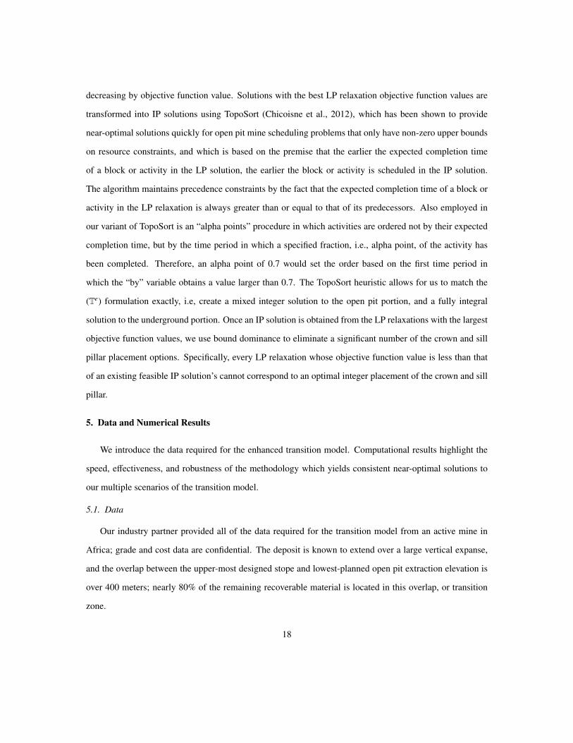
hundreds of millions of dollars depending on the crown pillar placement, and by tens of millions based on

the sill pillar placement. Our model provides not only a near-optimal solution, but identifies the economic

outcome of all possible crown and sill pillar placements.

Many mine operators defer underground mining until the open pit has finished production, resulting in

insufficient cash flow to justify an underground mine and an unmined portion of the deposit that could have

been extracted economically. By developing an efficient and tractable solution methodology, we can provide

mine operators with a tool to better understand the benefits of each transition elevation, and the ability to

confidently make a timely decision.

Additional work could address: (i) accuracy, (ii) applicability, and (iii) optimality gap. The accuracy

of the model would be improved with a better representation of the stockpiles. Since stockpiles contribute

significantly to the NPV, it would be beneficial to include mixing of ore in the stockpile and the degradation

of ore grade over time. The applicability of the model could be improved by adding blending requirements

at the mill and non-zero lower bounds on the knapsack constraints, which can be vital to maintain proper

mill feed, but that would destroy the mathematical structure that the TopoSort heuristic relies on. Finally,

we wish to incorporate a branch-and-bound algorithm within the OMP Solver to reduce the optimality gap

for a fixed crown and sill pillar placement option.

7. Acknowledgments

Alexandra Newman and Barry King received funding from the Center for Innovation in Earth Science

and Engineering at the Colorado School of Mines, and from Alford Mining Systems. Marcos Goycoolea

received funding from FONDECYT grant #1151098 and CONICYT PIA Anillo grant 1407. The authors

acknowledge Monica Dodd, Chris Alford, Xiaolin Wu, Hongliang Wang, Ralf Kintzel, Conor Meagher, and

many others for their continued support of and advocacy for this project. This research benefited significantly

from suggestions made by Daniel Espinoza (Universidad de Chile), Eduardo Moreno (Universidad Adolfo

Ibanez), Orlando Rivera (Universidad Adolfo Ibanez), and Andrea Brickey (South Dakota School of Mines).

25

C. Alford. Optimisation in underground mining. In Handbook of Operations Research in Natural Resources.

2007.

C. Alford. Optimization in underground mine design. PhD thesis, University of Melbourne, 2006.

A. Alonso-Ayuso, F. Carvallo, L.F. Escudero, M. Guignard, J. Pi, R. Puranmalka, and A. Weintraub. Medium

range optimization of copper extraction planning under uncertainty in future copper prices. European

Journal of Operational Research, 233(3):711–726, 2014.

AMPL Optimization LLC. Version 20140908, 2014. www.ampl.com.

O. Araneda. Opportunities and Challenges of the Transition from an Open Pit to an Underground Operation

in the Chuquicamata Mine. Presentation, Mine Planning 2015, Antofagasta, Chile, 2015.

M. Ataee-Pour. A Heuristic Algorithm to Optimise Stope Boundaries. PhD thesis, University of Wollongong,

2000.

E. Bakhtavar, K. Shahriar, and K. Oraee. A model for determining the optimal transition depth over from

open-pit to underground mining. 5th International Conference and Exhibition on Mass Mining, 2008.

D. Bienstock and M. Zuckerberg. Solving LP relaxations of large-scale precedence constrained problems.

Integer Programming and Combinatorial Optimization, 6080(1):1–14, 2010.

A. Bley, N. Boland, G. Froyland, and M. Zuckerberg. Solving mixed integer nonlinear programming prob-

lems for mine production planning with stockpiling. Optimization Online, Preprint:1–30, 2012.

M. Brazil and D.A. Thomas. Network optimization for the design of underground mines. Networks, 49(1):

40–50, 2007.

A. Brickey. Underground production scheduling optimization with ventilation constraints. PhD thesis,

Colorado School of Mines, 2015.

M. Carlyle and C. Eaves. Underground planning at Stillwater Mining Company. Interfaces, 31(4):50–60,

2001.

26

R. Chicoisne, D. Espinoza, M. Goycoolea, E. Moreno, and E. Rubio. A new algorithm for the open-pit mine

production scheduling problem. Operations Research, 60(3):517–528, 2012.

J. Crawford and W. Hustrulid. Open Pit Mine Planning and Design. Society of Mining Engineers, 1st

edition, 1979.

R. Epstein, M. Goic, A. Weintraub, J. Catalan, P. Santibanez, R. Urrutia, R. Cancino, S. Gaete, A. Aguayo,

and F. Caro. Optimizing long-term production plans in underground and open-pit copper mines. Opera-

tions Research, 60(1):4–17, 2014.

A. Finch. Open pit to underground. International Mining, January:88–89, 2012.

M.E. Gershon. Mine scheduling optimization with mixed integer programming. Min. Eng. (Littleton, Colo.),

35(4):351–354, 1983.

H. Hamrin. Guide to Underground Mining Methods and Applications. Atlas Copco, 1st edition, 1997.

IBM CPLEX Optimizer. Version 12.4.0.0. 2013. http://www-01.ibm.com/

software/commerce/optimization/cplex-optimizer/.

T. Johnson. Optimum open pit mine production scheduling. Technical report, University of California,

Berkeley, 1968.

B. Lambert, A. Brickey, A. Newman, and K. Eurek. Open pit sequencing formulations: A tutorial. Interfaces,

62(3):127–142, 2014.

H. Lerchs and Grossman. Optimum design of open-pit mines. Canadian Institute of Mining Bulletin, 58:

47–54, 1965.

M. Martinez, and A. Newman. A solution approach for optimizing long- and short-term production schedul-

ing at LKABs Kiruna mine. European Journal of Operational Research, 211(1):184–197, 2011.

Minemax. Mine Planning and Scheduling Solutions. 2013. www.minemax.com.

E. Moreno, M. Rezakhah, A. Newman, and F. Ferreira. Linear models for stockpiling in open-pit mining

production scheduling problems. Working Paper, 2016.

27

G. Munoz, D. Espinoza, M. Goycoolea, E. Moreno, M. Queyranne, and O. Rivera. Production scheduling

for strategic open pit mine planning, part I: A mixed integer programming approach. Working Paper,

2015.

A. Newman, and M. Kuchta. Using aggregation to optimize long-term production planning at an under-

ground mine. European Journal of Operational Research, 176(2):1205–1217, 2007.

A. Newman, E. Rubio, R. Caro, and A. Weintraub. A review of operations research in mine planning.

Interfaces, 40(3):222–245, 2010.

A. Newman, C. A. Yano, and E. Rubio. Mining above and below gorund: Timing the transition. IIE

Transactions, 45(8):865–882, 2013.

M. Osanlo, J. Gholamnejed, and B. Karimi. Long-term open pit mine production planning: a review of

models and algorithms. International Journal of Mining, Reclamation, and Environment, 22(1):3–35,

2008.

D. O’Sullivan. An optimization-based decomposition heuristic for solving complex underground mine

scheduling problems. PhD thesis, Colorado School of Mines, 2013.

D. O’Sullivan, and A. Newman. Optimization-based heuristics for underground mine scheduling. European

Journal of Operational Research, 241(1):248–259, 2015.

J. Picard. Maximal closure of a graph and applications to combinatorial problems. Management Science, 22

(11):1268–1272, 1976.

C. Qinglin, B. Stillborg, and C. Li. Optimisation of undergound mining methods using grey theory and

nerual networks. Balkema, Rotterdam, 1996. Mine Planning and Equipment Selection Conference.

S. Ramazan. The new fundamental tree algorithm for production scheduling of open pit mines. European

Journal of Operational Research, 177(2):1153–1166, 2007.

M. S. Shishvan, and J. Sattarvand. Long term production planning of open pit mines be any colony opti-

mization. European Journal of Operational Research, 240(3):825–836, 2015.

28

J. F. Souza, I. M. Coelho, S. Ribas, H. .G Santos, and L. H. C. Merschmann. A hybrid heuristic algo-

rithm for the open-pit-mining operational planning problem. European Journal of Operational Research,

207(2):1041–1051, 2010.

E. Topal, and S. Ramazan. A new MIP model for mine equipment scheduling by minimizing maintenance

cost. European Journal of Operational Research, 207(2):1065–1071, 2010.

L. Trout. Formulation and Application of New Underground Mine Scheduling Models. PhD thesis, The

University of Queensland, 1997.

R. Underwood, and B. Tolwinski. A mathematical programming viewpoint for solving the ultimate pit

problem European Journal of Operational Research, 107(1):96–107, 1998.

Whittle Consulting. Whittle consulting global optimization software, 2013.

http://www.whittleconsulting.com.au/.

29

8. Appendix

We demonstrate here computationally that, for the scenarios we examine, the LP relaxation of the basic

transition model (Tb) is weak relative to that of the enhanced transition model (Te), and we compare LP

solution times across standard algorithms. We also show that CPLEX is unable to solve the basic transition

model (Tb) for any scenario, i.e., that the basic transition model is intractable when solved with CPLEX.

Furthermore, two proofs – one each for the special knapsack and inventory balance constraints (see §3) –

show that our reformulations are no weaker than the original ones; moreover, computational results show

that the reformulations are strictly stronger.

8.1. Solutions to the Basic Transition Model (Tb)

Table 4 provides specific information regarding algorithmic performance and solution quality for our ten

test scenarios. We first compare solution times for standard LP algorithms when used to solve (Tb). All

computations were run on the same server as the enhanced transition model (Te). The barrier outperforms

the best version of simplex in all cases; the academic nature of the OMP Solver precludes it from handling

the complexity in the basic transition model, (Tb), in particular, the decisions regarding crown and sill pillar

placement (hence, our ad-hoc branch-and-bound strategy). Despite the ability of CPLEX (Version 12.6.0.0

using default parameter settings other than turning on memory emphasis) to solve the LP relaxation of (Tb),

the complexity of the problem proves intractable when seeking a good, integer-feasible solution. For all our

scenarios, CPLEX exhausts a 40,000-second time limit or runs out of memory before a solution within 5%

of optimality is found. We attribute this poor performance, in part, to the weak LP bound (as seen with a

comparison of the scaled net present values in the penultimate and last columns of Table 4). By contrast,

the results we obtain from using our reformulations and solution procedure on (Te) result not only in tighter

bounds, but also in near-optimal integer solutions, the latter stemming in large part from the the mathematical

structure of (Te) our TopoSort heuristic is able to exploit. The values for the tight LP relaxation solution

we obtain from (Te) in Table 4 result from the fixed crown and sill pillar combination that gives the best

objective function value for that scenario.

30

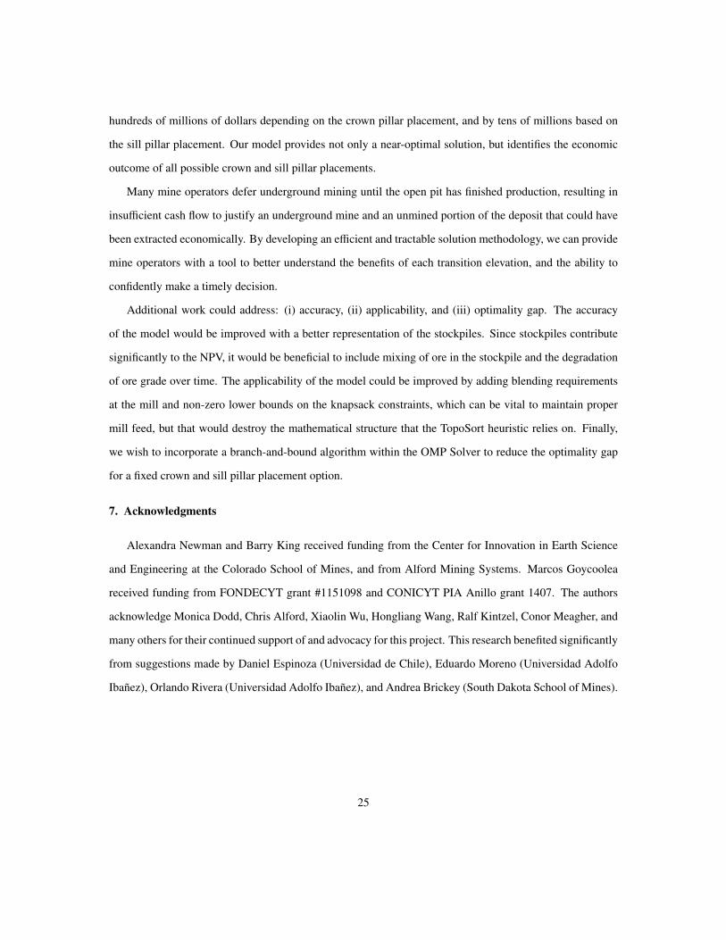
Table 4: (Basic and Enhanced Comparison) Comparison of solution times and solutions gaps between the basic transition model (Tb)and the enhanced transition model (Te) using CPLEX.

Scenario LP Solution Time for (Tb) (sec) IP Solution (Tb) LP Largest (Te)Barrier Simplex? Time (sec) Value LP Value

1 373.98 10343.09 † 3.20 2.722 359.53 8222.94 † 3.11 2.663 992.07 13821.83 ‡ 2.71 2.554 333.09 13163.29 ‡ 3.11 2.705 300.37 7451.82 † 3.20 2.706 338.96 8018.63 † 3.09 2.647 407.66 7792.96 † 3.01 2.588 756.81 25526.81 ‡ 2.71 2.559 383.78 8240.55 ‡ 6.24 4.86

10 369.52 7738.03 † 2.19 2.06?CPLEX is allowed to choose the variant of simplex to use, which results in employing dual simplex on the dualproblem† CPLEX was unable to produce an integer solution within 5% gap before running out of memory‡CPLEX was unable to produce an an integer solution within 5% gap before the 40,000 second limit of the LPrelaxation before running out of memory

8.2. On the strength of the Special Knapsack reformulation

In this section, we prove that the reformulation of the special knapsack constraints (1j), presented in

Section 3.1, is not weaker than the original formulation.

For simplicity, but without loss of generality, we consider the case of a single phase. For notation

purposes, assume that the blocks in the phase are numbered 1, . . . , |B| and that there is a limit of k blocks

that can be extracted in a given time period. (In Section 3.1, this term is represented as r). We assume

variables xbt are defined as before:

xbt =

1 if block b is extracted by time t

0 otherwise.

We can model the bound of k extractable blocks in a time period either by adding the knapsack constraint:

|B|∑b=1

(xbt − xb,t−1) ≤ k,∀t ∈ T 3 t > 1 (11)

or by adding precedence constraints:

xbt ≤ xb−k,t−1 ∀b ∈ B 3 b ≥ k + 1, t ∈ T 3 t > 1. (12)

We now show that (12) is at least as strong as (11).

31

Lemma Let X be the set of xbt variables such that:

xbt ≤ xb−1,t ∀t, b ∈ B 3 b ≥ 1 (13a)

xbt ≤ xb,t+1 ∀b ∈ B, t ≤ |T | − 1 (13b)

0 ≤ xbt ≤ 1 ∀b ∈ B, t ∈ T . (13c)

For sets:

P1 = {x ∈ X :|B|∑

b=1

(xbt − xb,t−1) ≤ k ∀t ∈ T }

P2 = {x ∈ X : xbt ≤ xb−k,t−1 ∀b ∈ B 3 b ≥ k + 1, ∀t ∈ T }

we wish to show that P2 ⊆ P1.

Proof.

We show that if xbt satisfies (12), then xbt satisfies (11). For each t ∈ T :

|B|∑b=1

(xbt − xb,t−1) =

k∑b=1

xbt −

|B|−k∑b=1

xb,t−1 +

|B|∑b=k+1

xbt −

|B|∑b=|B|−k+1

xb,t−1

≤

k∑b=1

xbt −

|B|−k∑b=1

xb,t−1 +

|B|∑b=k+1

xb−k,t−1 −

|B|∑b=|B|−k+1

xb,t−1

=

k∑b=1

xbt −

|B|−k∑b=1

xb,t−1 +

|B|−k∑b=1

xb,t−1 −

|B|∑b=|B|−k+1

xb,t−1

=

k∑b=1

xbt −

|B|∑b=|B|−k+1

xb,t−1

≤

k∑b=1

xbt

≤ k �

Combining the first and last expressions implies that|B|∑

b=1(xbt−xb,t−1) ≤ k. The reformulation of the special

knapsack constraints is done not only to enable the model to be more easily solved within a framework

the OMP Solver can handle, but also to improve the upper bound. For (S), the reformulation does not

improve the LP solution time over that obtained with the original model when using the OMP Solver for

32

both formulations; however, for the scenarios we test, the LP bound for (S) improves with the reformulation

by approximately 10%.

8.3. Inventory Balance Reformulation as Variable Substitution

In this subsection, we show that the reformulation of the inventory balance constraints (6) and the cor-

responding variable substitutions into expressions (7)-(9) presented in Section 3.2, is not weaker than the

original formulation. To this end, it suffices to show that for every integer-feasible solution of the reformu-

lation, there exists a corresponding feasible solution to the original formulation having the same objective

function value. Given a solution YSbt, ZSnbt of the reformulation, we construct a feasible solution in the original

space via the following linear mapping:

ISnbt = YSb,t−1 − ZSnb,t−1 ∀b ∈ B, n ∈ Nb, t ∈ T

IS−nbt = ZSnbt − ZSnb,t−1 ∀b ∈ B, n ∈ Nb, t ∈ T

YSnb2t = YSbt ∀b ∈ B, n ∈ Nb, t ∈ T

YSnb1t = 0 ∀b ∈ B, n ∈ Nb, t ∈ T

YSnb3t = 0 ∀b ∈ B, n ∈ Nb, t ∈ T

That is, substituting into (S) the expressions on the right-hand-side of the mapping for the variables listed

on the left-hand side results in true statements for each relevant set of constraints. (Constraints containing

only variables not involved in the mapping remain unchanged.) This implies that the solution involving YSbt

andZSnbt is feasible, and therefore valid, for (S). The same type of substitution, and the correct interpretation

of the new variables YSbt and ZSnbt yeilds the same objective function value as in the original formulation.

33