Optimizing Store-Brand Choices with Retail Competition

and Sourcing Options

By

Bo Liao

A dissertation submitted in partial satisfaction of the

requirements for the degree of

Doctor of Philosophy

in

Business Administration

in the

Graduate Division

of the

University of California, Berkeley

Committee in charge:

Professor Candace A. Yano, Chair

Professor Pnina Feldman

Professor Ying-Ju Chen

Spring 2014

Abstract

Optimizing Store-Brand Choices with Retail Competition and Sourcing Options

by

Bo Liao

Doctor of Philosphy in Business Administration

University of California, Berkeley

Professor Candace A. Yano, Chair

Retailers are introducing new store brands at a rapid pace, and annual sales of store brandsin the U.S. now exceeds $108 billion. In the literature on store brand decisions, it is com-monly assumed that (1) the retailer is a downstream monopolist; (2) either the store brandquality level is �xed, or, the marginal cost of production is constant and independent of thequality level of the store brand; and (3) the retailer either produces the store brand in-house,or sources it from a non-strategic manufacturer. Although these assumptions signi�cantlysimplify the analysis, they do not capture what is commonly seen in practice. As a conse-quence, the insights from these studies may not apply more broadly. Assumption (1) needsto be relaxed in order to study retailers' product assortment decisions (in terms of storeand national brands) and related pricing decisions at two competing retailers, along withpricing decisions of a leading national brand manufacturer. Assumption (1) and (2) need tobe simultaneously relaxed in order to investigate a retailer's store brand quality-positioningdecision when facing competition from another retailer that already carries a store brand.Assumptiona (2) and (3) need to be relaxed simultaneously in order to study how a re-tailer's optimal quality-positioning strategy changes across various sourcing arrangementsand various pricing power relationships among retailers and manufacurers. This disserta-tion contributes to the store brand literature by analyzing models based on more realisticassumptions than those in the literature.

This dissertation consists of three stand-alone papers. The �rst paper (in Chapter 2) inves-tigates a retailer's product assortment and pricing problem when she has the option to carrya store brand, a national brand, or both. I compare her decision when she is a downstreammonopolist and when she faces competition from another retailer who may also o�er the samenational brand and a competing store brand. Speci�cally, I assume the quality levels of theproducts are exogenous and analyze a manufacturer-Stackelberg game involving a nationalbrand manufacturer and two competing retailers. The national brand manufacturer sets awholesale price for the national brand product (the same for both retailers; I assume theyare similar in size and can therefore secure the same wholesale price). Then, observing thewholesale price, the retailers engage in a Nash game in which they set the retail prices for theproduct(s) they choose to carry. Finally, customers decide whether and what to purchase.Customers are heterogeneous in two dimensions: location, which can be interpreted as thedegree of loyalty to one retailer or the other, and willingness to pay per unit of quality. Eachcustomer visits the retailer where he can obtain the maximum surplus (willingness to payless purchasing and transportation costs) among the o�ered products. After the customer

1

arrives at the selected retailer, the transportation cost is now sunk, so he buys the o�eredproduct with the larger di�erence between his willingness to pay for the product and itsprice, if it is non-negative.

The second paper (in Chapter 3) addresses store brand quality-positioning decisions for re-tailers facing retail competition. Speci�cally, I assume one of the two retailers (Retailer 2)already carries a store brand product whose quality level is �xed, and both retailers mayo�er the national brand product with a �xed quality level. The representation of customerpreferences and the resultant demands are the same as in the �rst paper. I model the dynam-ics via a two-stage game. In the �rst stage, Retailer 1 decides whether to introduce a storebrand product, and if so, its quality level. Then the three parties engage in a manufacturer-Stackelberg pricing game. Finally, customers decide whether and what to purchase. In the�rst stage, Retailer 1 anticipates the outcome of the second-stage game. I analyzed thesecond stage game in the �rst paper; it is a subproblem in the second paper. I also analyzea setting in which both retailers may choose the quality levels of their store brand productssimultaneously.

The third paper (in Chapter 4) studies a retailer's equilibrium quality-positioning strategyunder three sourcing structures, and for each sourcing structure, I consider three types ofchannel price leadership. Speci�cally, I study games between (among) a retailer, a nationalbrand manufacturer and a strategic third-party manufacturer, where applicable. The retailercarries a product (with a �xed quality) o�ered by the national brand manufacturer, and isconsidering introducing a store brand whose quality can be decided. Customers are hetero-geneous in their willingness-to-pay (WTP) per unit of quality. The utility a customer derivesfrom either product equals her WTP per unit of quality times the product quality. Eachcustomer chooses the product that gives her the greatest surplus (utility less price), providedthat it is non-negative. The unit production cost of both products is strictly convex andincreasing in the quality level of the product. I derive the retailer's equilibrium store-brandquality decision under three sourcing arrangements and three pricing power scenarios. Thethree sourcing arrangements are in-house (IH), a leading national brand manufacturer (NM)(whose product the retailer also carries), and a strategic third-party manufacturer (SM). Thethree power scenarios are the ones most commonly seen in the literature: Manufacturer-Stackelberg (MS), Retailer-Stackelberg (RS), and Vertical Nash (VN). In sum, I examinenine (i.e., three times three) combinations of sourcing and pricing power (or �game�) scenar-ios, and compare the retailer's optimal quality positioning decision and other equilibriumresults (including prices) across the nine scenarios. In all nine combinations of sourcing andpricing power scenarios, the retailer moves �rst in setting the quality of her store-brand (dur-ing the product development phase) before any pricing decisions are made. I derive subgameperfect equilibria for all scenarios. To the best of my knowledge, I am the �rst to present acomparison of equilibria for these nine realistic combinations of sourcing and pricing powerin this context.

This dissertation makes several contributions to the literature on store brand strategies.First, the majority of papers on store brand strategies consider a monopolist retailer. Thefew papers that consider retail competition are based on restrictive assumptions concerningfactors such as product quality (e.g., assuming store brand products have equal quality levels)

2

or product o�ering (e.g., both retailers must o�er the national brand product). My workin papers 1 and 2 takes a �rst step in presenting a model that is general enough to allowme to study retailers' strategies in a context with store and national brands, and with retailcompetition. Second, prior research utilizes demand models that are limited in their abilityto capture customers' joint selection of a retailer and a product. My work in papers 1 and2 is based on a model of customer preferences that allows me to incorporate both qualitydi�erentiation among the products and the degree of customer loyalty to retailers, both ofwhich are important in my problem context. This model is �exible enough to support afairly rich representation of demands. Third, in paper 3, I take a �rst step in studying theinteraction between store-brand sourcing and positioning decisions, and the interplay of thesedecisions with the retailer's pricing power. From a comparison of the retailer's equilibriumstore brand quality levels for the nine combinations of sourcing and game structure, I obtaina full characterization of the ordering of store-brand quality, retailer's pro�t, retail prices andconsumer welfare across the nine combinations. To the best of my knowledge, I am the �rstto present a comparison of equilibria for these nine realistic combinations of sourcing andpricing power in the store brand context. I also show that sourcing of store brands plays akey role in the competitive interaction between a retailer and a national brand manufacturer.Whereas the marketing and economics literatures have emphasized the role of store brandsin helping retailers elicit price concessions from national brand manufacturers, I �nd thathaving a preferable sourcing arrangement for a store brand product is more valuable thanhaving pricing power.

3

CHAPTER 1

Introduction

Store brands account for a sizable percentage of sales at retailers. In 2012, sales ofstore brands in U.S. supermarkets alone totaled $59 billion, with a store brand unit shareof 23.1% and a dollar share of 19.1% (PLMA, 2013). Furthermore, industry experts saythat store brand sales could double in the next �ve to six years (Watson, 2012). Storebrands help retailers in various ways. First, a store brand serves as a strategic weapon forthe retailer by increasing the retailer's bargaining strength, thereby eliciting wholesale pricereductions and non-price concessions from suppliers of competing products (Mills 1995 and1999; Narasimhan and Wilcox 1998; Gabrielsen and Sorgard 2007). Second, they serve asdi�erentiating tools that distinguish a retailer from its competitors (Corstjens and Lal 2000).Third, they help retailers to build store loyalty if customers repeatedly visit to purchase store-brand products, which are not available elsewhere (Bell et al. 1998). As a result, retailersactively engage in store brand development. As one example, Kroger is expanding its storebrand selection, and this is contributing to its bottom line (Associated Press, 2013). Asthe trend of increasing store brand development continues, managing store-brand productshas become more challenging for retailers. For this reason, this dissertation aims to providemanagerial insights for retailers carrying store brands and to help them optimize their storebrand strategies.

In the literature on store brand decisions, it is commonly assumed that (1) the retailer isa downstream monopolist; (2) either the store brand quality level is �xed, or, the marginalcost of production is constant and independent of the quality level of the store brand; and(3) the retailer either produces the store brand in-house, or sources it from a non-strategicmanufacturer. Very few papers are based on substantially more general assumptions. Al-though the commonly-adopted assumptions signi�cantly simplify the analysis, they do notcapture what is typically seen in practice. As a consequence, the insights from these studiesmay not apply more broadly. We elaborate on this point below.

First, retail competition has become increasingly intense in recent years. For example,in June 2012, a few days after Kroger announced its plan to launch its store brand co�eepods for Keurig machines, Safeway launched Safeway brand Keurig co�ee pods. In such ascenario, both retailers need to respond to their competitor's strategies, but the literaturehas little to say about how they should respond. To provide insights on this issue, one hasto relax assumption (1) above. Second, each retailer needs to determine its quality level.As an example, Kroger has a �three-tier� store brand positioning strategy. Not only doesKroger need to decide the tier of a new store-brand product, but even for a given tier,it needs to decide the quality level at a more detailed level. This decision will not onlya�ect the unit production cost Kroger incurs, but it will also a�ect the competitivenessof its store brand vis-a-vis competing national brand product(s) and the products sold atcompeting retailers. Assumptions (1) and (2) above need to be relaxed simultaneously inorder to investigate optimal strategies in this commonly-occurring situation. Third, some

1

store brands are sourced from large national brand manufacturers who also produce and o�ercompeting products, and some are sourced from third-party manufacturers that have marketpower. For example, in the UK, the store-brand cola at a large supermarket chain is producedby Coca-Cola (Berges-Sennou 2006). And Overhill Farms, a third-party producer known forprocessing frozen foods, has been producing store-brand products for some major retailers(Mercury News, March 2013). Many such �rms have gained considerable market presenceand power as the demand for store brand products has grown. Given the variety of possiblesourcing arrangements and the consequent variations in pricing power among the parties,one would think that the retailer's optimal choice of store brand quality should depend uponthese factors. For one to investigate how the optimal store brand quality depends upon thesefactors, assumptions (2) and (3) above need to be relaxed simultaneously.

This dissertation contributes to the store brand literature by addressing some of thelimitations of models in the literature that were mentioned above. Speci�cally, this disser-tation consists of three stand-alone papers. The �rst paper investigates a retailer's productassortment and pricing problem when she has the option to carry a store brand, a nationalbrand, or both. I compare her decision when she is a downstream monopolist and when shefaces competition from another retailer who may also o�er the same national brand and acompeting store brand. The second paper addresses store brand quality-positioning deci-sions for retailers facing retail competition. The third paper studies a retailer's equilibriumquality-positioning strategy under three sourcing structures, and for each sourcing structure,I consider three types of channel price leadership. In the third paper, I assume the retailer isa downstream monopolist in order to isolate the interaction between the positioning decisionand sourcing structure from the e�ect of retail competition.

Below, I present overviews of the models in the three papers. I primarily use analytic(game theoretic) approaches, and derive the equilibrium strategies for all parties participatingin the game. In the �rst paper, I assume the quality levels of the products are exogenous andinvestigate a manufacturer-Stackelberg game between a national brand manufacturer andtwo retailers. The national brand manufacturer sets a wholesale price for the national brandproduct (the same for both retailers; I assume they are similar in size and can therefore securethe same wholesale price). Then, observing the wholesale price, the retailers engage in a Nashgame in which they set the retail prices for the product(s) they choose to carry. Finally,customers decide whether and what to purchase. In the model, customers are heterogeneousin two dimensions: location, which can be interpreted as the degree of loyalty to one retaileror the other, and willingness to pay per unit of quality. In the �rst dimension, customersare distributed uniformly along a Hotelling line between the two retailers and they incur atransportation cost for visiting either retailer. Due to the transportation cost, customers aremore loyal to the nearer retailer and the degree of loyalty increases as the transportationcost per unit distance increases. In the second dimension, customers' willingness to payper unit of quality is uniformly distributed within an interval. Each customer visits theretailer where he can obtain the maximum surplus (willingness to pay less purchasing andtransportation costs) among the o�ered products. Here, each customer's willingness to payis obtained by multiplying his willingness to pay per unit of quality by the product's qualitylevel. Likewise, the customer's transportation cost is equal to the transportation cost perunit distance multiplied by the customer's distance from the respective retailer. After thecustomer arrives at the selected retailer, the transportation cost is now sunk, so he buys the

2

o�ered product with the larger di�erence between his willingness to pay for the product andits price, if it is non-negative.

In the second paper, I assume one of the two retailers (Retailer 2) already carries astore brand product whose quality level I assume to be �xed; and I investigate the otherretailer's (Retailer 1's) store brand introduction decisions, speci�cally with respect to productquality and price. Both retailers can also o�er the national brand and select its price. Thequality of Retailer B's store brand is �xed, but he can adjust its price. The representationof customer preferences and the resultant demands are the same as in the �rst paper. Imodel the dynamics via a two-stage game. In the �rst stage, Retailer 1 decides whether tointroduce a store brand product, and if so, its quality level. Then the three parties engagein a manufacturer-Stackelberg pricing game: the national brand manufacturer �rst sets awholesale price for his product and the retailers then engage in a Nash game in which theyset retail price(s). Finally, customers decide whether and what to purchase. In the �rststage, Retailer 1 anticipates the outcome of the second-stage game. I analyzed the secondstage game in the �rst paper; it is a subproblem in the second paper. In the second paper, Ifocus on Retailer 1's decision regarding her store brand quality and the implications of thatchoice for the various pricing decisions. I also explore characteristics of the equilibrium whenthe two competing retailers can simultaneously choose their store brand quality levels.

In the third paper, I study games between (among) a retailer, a national brand manu-facturer and a strategic third-party manufacturer, where applicable. The retailer carries aproduct (with a �xed quality) o�ered by the national brand manufacturer, and is consider-ing introducing a store brand whose quality can be decided. Customers are heterogeneousin their willingness-to-pay (WTP) per unit of quality. The utility a customer derives fromeither product equals her WTP per unit of quality times the product quality. Each customerchooses the product that gives her the greatest surplus (utility less price), provided that it isnon-negative. The unit production cost of both products is strictly convex and increasing inthe quality level of the product. I derive the retailer's equilibrium store-brand quality decisionunder three sourcing arrangements and three pricing power scenarios. The three sourcing ar-rangements are in-house (IH), a leading national brand manufacturer (NM) (whose productthe retailer also carries), and a strategic third-party manufacturer (SM). The three power sce-narios are the ones most commonly seen in the literature: Manufacturer-Stackelberg (MS),Retailer-Stackelberg (RS), and Vertical Nash (VN). Under MS, the national-brand manu-facturer sets a wholesale price �rst, followed by the SM, where applicable. Under RS, theretailer sets her margin for the store- and the national brands before the manufacturer(s)set their wholesale prices. Under VN, the retailer and the manufacturer(s) engage in a Nashgame, in which the retailer sets her margins while the manufacturer(s) set the wholesaleprices. In sum, I examine nine (i.e., three times three) combinations of sourcing and pricingpower (or �game�) scenarios, and compare the retailer's optimal quality positioning decisionand other equilibrium results (including prices) across the nine scenarios. In all nine combi-nations of sourcing and pricing power scenarios, the retailer moves �rst in setting the qualityof her store-brand (during the product development phase) before any pricing decisions aremade. I derive subgame perfect equilibria for all scenarios. To the best of my knowledge,I am the �rst to present a comparison of equilibria for these nine realistic combinations ofsourcing and pricing power in this context.

This dissertation makes several contributions to the literature on store brand strategies.First, the majority of papers on store brand strategies consider a monopolist retailer. The

3

few papers that consider retail competition are based on restrictive assumptions concerningfactors such as product quality (e.g., assuming store brand products have equal quality levels)or product o�ering (e.g., both retailers must o�er the national brand product). My workin papers 1 and 2 takes a �rst step in presenting a model that is general enough to studyretailers' strategies in which store brands and national brands compete in the presence ofretail competition. Second, prior research utilizes demand models that are limited in theirability to capture customers' joint selection of a retailer and a product. My work in papers 1and 2 is based on a model of customer preferences that allows me to incorporate both qualitydi�erentiation among the products and the degree of customer loyalty to retailers, both ofwhich are important in my problem context. This model is �exible enough to support afairly rich representation of demand. Third, in paper 3, I take a �rst step in studying theinteraction between store-brand sourcing and positioning decisions, and the interplay of thesedecisions with the retailer's pricing power. From a comparison of the retailer's equilibriumstore brand quality levels for the nine combinations of sourcing and game structure, I obtaina full characterization of the ordering of store-brand quality, retailer's pro�t, retail prices andconsumer welfare across the nine combinations. To the best of my knowledge, I am the �rstto present a comparison of equilibria for these nine realistic combinations of sourcing andpricing power in the store brand context. I also show that sourcing of store brands plays akey role in the competitive interaction between a retailer and a national brand manufacturer.Whereas the marketing and economics literatures have emphasized the role of store brandsin helping retailers elicit price concessions from national brand manufacturers, I �nd thathaving a preferable sourcing arrangement for a store brand product is more valuable thanhaving pricing power. Chapter 5 provides further details on the research contributions ofthis dissertation.

The remainder of the dissertation is organized as follows. Chapters 2, 3 and 4 containpapers 1, 2, and 3, respectively. In these three chapters, the equation, �gure and Appendixreferencing pertain to equations, �gures and Appendices within the same chapter. Chapter5 concludes the dissertation by summarizing the key results.

4

CHAPTER 2

Product Assortment and Price in the Presence of Retail

Competition and Store Brands

1. Introduction

Sales of store brands have grown rapidly over the past decade, with an annual increase of4.9% annually between 2009 and 2012 to over $108 billion annually. By comparison, sales ofnational brands have grown 2.1% annually during the same period (PLMA 2013a). Whatare the reasons underlying this trend? News articles and research reports suggest thereis a positive reinforcement cycle of store brand growth leading to retailers' investments instore brands, which then leads to further growth. Speci�cally, during the recent economicrecession, many consumers dropped national brands for store brands as they tightened theirbudgets. But once they switched, they tended not to switch back as they were �happy with�the new choices. Indeed, 46% of consumers think �it's foolish to spend more if comparablequality is available from a store brand� (Consumer Edge Insight 2011). And 97% of con-sumers favorably compared store brand products to their previous national brand choices(PLMA 2010).

Increased customer acceptance has bene�ted retailers, as their stores have become betterdi�erentiated because of store brands. Stronger store brands have helped them increasestore tra�c and build store loyalty (see, e.g., Corstjens and Lal 2000; Ailawadi et al. 2008).Recognizing the bene�ts, retailers continue to invest in quality, merchandising and spaceallocation for store brands. For example, Supervalu plans to increase its Essential Everydaystore brand o�erings to 2700 products by 2013 (Store Brand Decisions 2012). At Safeway,store brands can be found alongside competing national brands in categories �from dry cerealand frozen foods to paper towels and laundry detergent� (www.safeway.com). On its website,Safeway claims that the store brands are �the same as national brands but at a much lowerprice� (www.safeway.com).

An interesting case study concerning store brand assortment is the practice at TraderJoe's. As much as 80% of the products carried there in 2010 were store brands (Kowitt 2010)and this strategy has been successful. Signi�cantly, 92.6% of shoppers there reported theywere �not bothered� by the lack of national brands and many of them even objected to theaddition of national brands there. On a news webpage about Trader Joe's product o�erings,one customer commented, �Adding national brand products would be a huge mistake. Whyo�er a commodity you could purchase at any other retailer and therefore be at risk for `pricecomparison'?� (Thayer 2009).

A key element missing from this picture of competition between store and national brandsis retail competition. When retailers try to win over customers from their competitors byo�ering store brands, their competitors are likely to do the same. For example, in June 2012,a few days after Kroger announced its plan to launch its store brand co�ee pods for Keurigmachines, Safeway launched Safeway brand Keurig co�ee pods. (Kroger owns the Ralph's

5

supermarket chain that competes with Safeway in several major metropolitan areas.) Indeed,retail competition has become even more intense in recent years with the expansion of non-traditional advertising channels such as social media, which allow very rapid disseminationof prices, perceptions of quality, etc.

Retailers have begun to realize the need to consider retail competition when devising storebrand strategies. Notably, 12% of retailers reported that the primary reason they acceleratedstore brand development was the need to respond to expanded e�orts by their competitors(Canning and Chanil 2011). Retailers are expanding their store brands into new categories.Categories such as refrigerated and frozen foods were considered �unbrandable� by retailersyears ago, but now they are among the fastest-growing store brand categories (PLMA 2012).Retailers are also eliminating national brands from some product categories: 60% of retailersreported that they either already or were planning to eliminate some national brands to makeroom for their store brands (Canning and Chanil 2011). But questions remain. How exactlyshould a retailer adjust her store brand strategies, or when should she drop a national brand,in response to related strategies at her competitors? Moreover, how does retail competitiona�ect the pricing strategy and the pro�t of an upstream national brand manufacturer? Fewanalytical models exist to aid in answering these questions, and none considers the generalitythat our model o�ers.

We consider a setting with a manufacturer of a leading national-brand product and tworetailers. Each retailer can o�er the national-brand product and a competing store-brandproduct in the same product category. Each store brand is produced either in-house by theretailer or by a third-party manufacturer which is a non-strategic player in the game. Majorgrocery chains including Safeway and Kroger own manufacturing facilities that produce someof their store-brand products. Also, there are regional brand manufacturers that producestore brands for speci�c markets (PLMA 2013b) and do not have enough power to noticeablya�ect the outcome, except for a small markup over their variable costs. We leave scenarioswith strategic store brand producers or production of store brands by the national brandmanufacturer for future research.

We model the dynamics via a national brand manufacturer-Stackelberg game. First, thenational brand manufacturer sets a single wholesale price o�ered to both retailers, takingretailers' reactions into consideration. Typically, it is large retailers who are able to o�ertheir own store brands, so we assume that the retailers are of similar size and therefore thenational brand manufacturer needs to o�er them the same wholesale price. We assume theproducer(s) of the store brand(s) is (are) non-strategic players. Given the wholesale price,the two retailers engage in a Nash pricing game for the products they choose to o�er. If aretailer sets a su�ciently high price, this has the same e�ect as not carrying the product atall. In this way, retailers' pricing decisions endogenize their product assortment decisions.Finally, customers decide whether and what to purchase.

Customers are heterogeneous in two dimensions: location and willingness to pay per unitof quality. In the �rst dimension, customers are distributed uniformly on a Hotelling linebetween two retailers and they incur a transportation cost for visiting each retailer, whichallows us to capture the degree of customer loyalty to one retailer or the other. In the seconddimension, customers' willingness to pay is uniformly distributed within an interval. Eachcustomer chooses a retailer to visit (if any) on the basis of which one o�ers the producto�ering the highest surplus (willingness to pay for the product less transportation cost lessprice). Upon arriving at the retailer, the transportation cost is sunk, so the customer then

6

purchases the product that provides the higher di�erence between the willingness to payfor the product and its price, as long as it is nonnegative. Groznik and Heese (2010) use asimilar model of demand; we explain the di�erences between their model and ours in moredetail later.

From our analysis of the model, we o�er insights into the following aspects of the equi-librium:

Product assortment at retailersWe study the product assortment and pricing problem facing competing retailers. We alsocompare how the retailer's decision di�ers under retail monopoly and duopoly settings. Notsurprisingly, we �nd that, ignoring the �xed cost of store brand introduction, a retailer shouldalways introduce her store brand unless the national brand manufacturer intentionally un-derprices the national brand to increase market share while ignoring pro�t considerations.There is also a threshold wholesale price for the national brand product above which theretailer does not o�er the national brand product. Surprisingly, although these thresholdwholesale prices di�er for the two retailers, under mild conditions on the customers' trans-portation cost (which re�ects the relative disutility of visiting the two retailers), for eachretailer, the threshold is the same whether she is a monopolist or whether she faces compe-tition from another retailer. If the national brand manufacturer o�ers a low wholesale price(below the smaller of the thresholds for two retailers), both retailers will o�er the nationalbrand. If the national brand manufacturer o�ers a high wholesale price (above the larger ofthe thresholds for the two retailers), neither retailer will o�er the national brand. Betweenthe two thresholds, only one retailer�the one with the store brand of lower quality�o�ersthe national brand. This implies that, as the wholesale price of the national brand increases,the retailer with the higher-quality store brand will stop o�ering the national brand earlier.This partly explains the product assortment practice at Trader Joe's: because the quality ofits own-label products is high, it does not carry national brands in as many categories as itscompetitors do.

Price gap between store and national brandsThe price gap between the national and store brands conveys the �value for the money� ofthe store brand, but it simultaneously signals the quality gap to consumers. Because ofthis, practitioners have been very interested in determining a good �price gap� between thenational and store brands.

Hoch and Lodish (1998) conducted a study of consumer's attitude toward prices of prod-ucts in the analgesics category. Their results show that the price gap does not a�ect theconsumers' choice of stores. Instead, only the price levels of the national and store brands ata retailer (compared to prices at the retailer's competitors) matter. Moreover, the nationalbrand price matters more in customers' overall store choice probability. The authors thusrecommended that retailers �gure out whether their current prices are above or below thetheoretical optimal values.

Our research can be used to aid in determining optimal prices for the national and storebrands for a retailer under competition. From our equilibrium results, we also �nd thatretailers should respond to competition by lowering the prices of both the store and nationalbrands, and should lower the price of the national brand to a greater extent. In other words,in the face of competition, retailers experience greater pressure on their price for the national

7

brand than on their price for store brands. This parallels the empirical �ndings of Hoch andLodish.

National brand manufacturer's product distributionThe launch of the store brand co�ee pods for Keurig machines described earlier caused thestock price of Green Mountain, a national brand, to plummet (Geller 2012). Thus, it isimportant for the national brand manufacturer to develop counterstrategies. A key questionis: when both retailers o�er store brands, should a national brand manufacturer sell throughonly one or both retailers?

We �nd that the answer to this question depends on the quality disparity between thetwo store brands. When the quality disparity is low, the national brand manufacturer pricesin such a way that both retailers continue to sell the national brand. But when the qualitydisparity is greater than a threshold, the national brand manufacturer prices so that onlythe retailer with the lower store brand quality continues to o�er the national brand product.

Sethuraman (2009) points out that few analytical papers derive results regarding nationalbrand counterstrategies when facing competition from store brands; one notable exception isMills (1999). Our work contributes to our understanding along these lines by characterizing,as part of our analysis of a three-party game, the national brand's optimal strategies andhow they change as costs, product quality, and market parameters change.

E�ect of customer loyaltyMany large retail chains invest heavily in customer loyalty programs; virtually every majorgrocery and drug store chain has one. What is the e�ect of greater customer loyalty inour environment? We �nd that when customers exhibit no loyalty, retailers end up in aprisoner's dilemma: both of them prefer a situation in which neither of them carries thenational brand product. But at the equilibrium, both of them carry it, yet the perfectlycompetitive environment leads both of the retailers to price the national brand at cost, soall of their pro�t comes from their store brands.

The remainder of this paper is organized as follows. We review the related literaturein Section 2. Our model is presented in Section 3. In Section 4, we present each retailer'sproblem of choosing her product assortment and prices, and properties of the equilibriumbetween the retailers for a given wholesale price of the national brand product. In Section5, we analyze and discuss the national brand manufacturer's optimal pricing policy, whichdetermines which retailer(s) choose to o�er the national brand. A discussion of special casesand extensions appears in Section 6. We conclude the paper in Section 7.

2. Literature Review

The literature on competition between national and store brands is extensive but, asmentioned earlier, very few analytical models consider competition between retailers, nordo they consider di�erential quality of the store brand products or loyalty of customers tothe retailers. In the interest of completeness, we �rst provide a comprehensive high-leveloverview of analytical (equilibrium) models of national- and store-brand competition. Nearthe end of this section, we provide more detail on the few papers that are closely-related toours.

8

A major stream within the literature on store brands investigates the strategic bene�tsthat retailers can gain from them. First, a store brand serves as a strategic weapon forthe retailer by increasing the retailer's bargaining strength, thereby eliciting wholesale pricereductions and non�price concessions (Du et al. 2005, Mills 1995, Narasimhan and Wilcox1998, Mills 1999, Pauwels and Srinivasan. 2004, Steiner 2004, Tarziján 2004, Gabrielsenand Sørgard 2007). Second, store brands can be instruments for retailers to enhance storedi�erentiation and store loyalty (Corstjens and Lal 2000, Sudhir and Talukdar 2004, Aveneland Caprice 2006, Geylani et al. 2009). Third, a store brand can help a retailer to betterdiscriminate among consumers by serving as one additional product version in its category(Wolinsky 1987, Soberman and Parker 2004, Soberman and Parker 2006). Finally, retailersmay carry a store brand because they have more control over its positioning and production(Bergès-Sennou and Rey 2008, Scott-Morton and Zettelmeyer 2004). We are most interestedin the role of store brands as a retailer's strategic weapon in the vertical interaction withnational brand manufacturers, particularly under retail competition.

We �rst discuss analytical models of the e�ect of store-brand introduction on nationalbrand wholesale prices. These models are based on a manufacturer-Stackelberg game be-tween a national brand manufacturer and one retailer whose store-brand product is availableat a constant marginal cost. Under the assumption that the national brand manufacturerand the store brand producer share the same constant marginal cost, Mills (1995, 1999) �ndsthat the wholesale price o�ered by the national brand manufacturer decreases as the qualityof the store brand increases. When the quality of the store brand is not too low, the optionof carrying a store brand imposes a threat, so the national brand manufacturer o�ers a lowerwholesale price than when the retailer does not have a store-brand option and thereby suc-cessfully forecloses the store brand. If the quality of the store brand is very high, the storebrand is sold, and as the quality of the store brand rises, the national brand manufacturerdecreases its wholesale price to provide an incentive for the retailer to sell a fair amount ofthe national brand instead of the store brand alternative.

Unlike Mills, Bontems et al. (1999) �nd that the wholesale price is not necessarily mono-tonically decreasing in the quality of the store brand when the unit production cost is convexand increasing with its quality. This is because the store brand su�ers from a cost disadvan-tage when its quality exceeds a threshold, so it no longer imposes a threat. Both Narasimhanand Wilcox (1998) and Gabrielsen and Sørgard (2007) consider a model with two customersegments: one is loyal to the national brand and the other (so-called �switchers�) may choosethe store brand if the price is attractive. Narasimhan and Wilcox (1998) assume that bothsegments have the same reservation price for the store and national brands, and obtainresults that indicate the introduction of a store brand can only lead to a decrease in thenational-brand wholesale price. Gabrielsen and Sørgard (2007) assume the loyal customershave a higher willingness to pay for quality, and their analysis indicates that the introductionof the store brand can lead to either an increase or a decrease in the wholesale price of thenational brand, depending on the fraction of loyal customers. Soberman and Parker (2004,2006) treat the level of advertising for the national brand as a decision variable and showthat the direction of change in the average price for the product category after the storebrand is introduced depends on whether advertising is expensive (with respect to its abilityto increase the utility of the national brand among brand seekers). Fousekis (2010) considersa three-stage game in which the national brand manufacturer and retailer simultaneously setthe quality level of their respective product (within a range) in the �rst stage of the game;

9

the author assumes the store brand quality is lower than that of the national brand. In thesecond stage, the national brand manufacturer chooses a wholesale price, and in the �nalstage the retailer sets prices. Consumers are heterogeneous in their willingness to pay perunit of quality and choose the product that gives them a higher surplus, if it is non-negative.He shows that, under his assumptions, it is optimal for both parties to choose the highestfeasible quality level for their respective products.

Characteristics of vertical channel structures in the presence of store brands are also per-tinent to our research. There are many analytical models of traditional vertical interactionsbetween manufacturers and retailers (McGuire and Staelin 1983, Shugan 1985, Choi 1991,Lee and Staelin 1997), but we are not aware of any that address the speci�c characteristics ofcompetition between store and national brands There is, however, substantial empirical re-search on the nature of competition between store and national brands, which suggests thatthe type of interaction and the degree of competition between national and store brands isidiosyncratic across categories: it depends on whether or not the national brand is a leadingproduct as well as the quality of the store brand. See Putsis and Dhar (1998), Cotterill andPutsis (2000), Sayman et al. (2002), Meza and Sudhir (2010) and the references therein.

How do consumers choose among di�erent stores? A rich stream of empirical researchaddresses this questions. Bell et al. (1998) develop and test an empirical model to investigatethe store choice behavior of households visiting a set of stores over a certain time horizon,based on the assumption that each shopper is most likely to visit the store with the lowesttotal shopping cost. They �nd that, in order to provide a comprehensive theory of storechoice, both �xed and variable costs are necessary. The �xed cost is the cost independentof the shopping list whereas the variable cost depends on the shopping list. The �xed costdepends upon the travel distance, the shopper's inherent preference for the store, and historicstore loyalty, whereas the variable cost is the total expected cost of the items on the shoppinglist if purchased at the store.

A stream of research also examines how customers perceive store brands. Richardsonet al. (1996) �nd that customers' reliance on extrinsic cues (such as price, packaging, andbrand) adversely a�ects customers' propensity to purchase store brands. Baltas and Argous-lidis (2007) �nd that quality plays a major role in the evaluation process from consumersdevelop their store brand preferences. Sayman et al. (2002) �nd that store brands are viewedas slightly more similar to secondary national brands than to the leading national brand. deWulf et al. (2005) �nd that national brands enjoy brand equity while store brands do not.

Next, we review analytical models of demand when store and national brand(s) compete.In the literature, there are roughly �ve groups of demand models developed for such acontext. Models in the �rst group derive demand from one representative consumer, orequivalently, by assuming consumers are homogenous (cf. Choi and Coughlan 2006 andBergès-Sennou and Rey 2008). The second group of models uses an aggregate demandfunction which is linear with respect to price and is parameterized by di�erentiation andsubstitution factors (cf. McGuire and Staelin 1983, Choi 1991, Raju et al. 1995, Cotterilland Putsis 2000 and Sayman et al. 2002). Linear demand functions allow researchers toconduct sensitivity analysis on the cross-price sensitivity parameters and examine how theya�ect the equilibrium channel structure. However, linear demand functions are limited intheir ability to accommodate the combination of complex customer choice behavior andinteractions among multiple parties in a vertical channel.

10

The third group of models derives demand from individual utility functions of customers,which are assumed to be increasing with product quality and the customer's willingness topay for quality, and decreasing with the product price (cf. Mills (1995 and 1999), Bontemset al. 1999, Tarziján 2004 and Avenel and Caprice 2006). When such a utility function isused, the store- and the national brands are assumed to di�er in their quality levels, and theconsumers' willingness to pay for quality varies among consumers (a uniform distributionis usually assumed). The fourth group of models segments customers into those who areloyal to the national brand and those who are more willing to switch (cf. Narasimhanand Wilcox 1998, Gabrielsen and Sørgard 2007, Soberman and Parker 2004, Soberman andParker 2006 and Corstjens and Lal 2000). Articles in this group examine the role of storebrand introduction and study how the equilibrium changes in response to a change in segmentsizes. Finally, the remaining models do not fall into any of the above categories and are morecontext-speci�c (e.g., Scott-Morton and Zettelmeyer 2004, Du et al. 2005 and Bergès-Sennou2006).

There has been little analytical research that incorporates retail competition when bothnational- and store-brand products are o�ered and the national brand manufacturer is astrategic player. Indeed, in a recent survey paper by Sethuraman (2009) on models ofnational- and store-brand competition, only one article with retail competition is mentioned(Corstjens and Lal (2000)), which we discuss later in this section. We o�er a few commentson relevant articles, including those published after 2009, here. First, we discuss articles inwhich the retailer does not have an explicit product assortment decision. In the model ofChoi and Fredj (2013), two retailers both o�er the national brand and their respective storebrand, so there is no product assortment decision. The authors assume there is competitionbetween the store- and national-brand at each retailer, but there is very little price com-petition between the store brands (which is a salient feature of our model). They deriveequilibrium prices under manufacturer-Stackelberg, Vertical Nash, Retailer Stackelberg andRetailer Double Stackelberg (in which one retailer moves �rst, then the other retailer, then�nally the national brand manufacturer). They provide a comparison of various parties'pro�ts under the four channel leadership arrangements. In general, the �ndings are similarto others in the literature: the retailers bene�t from greater leadership but the nationalbrand manufacturer is not necessarily better o� being the leader.

Corstjens and Lal (2000) analyze a two-period setting with two retailers who o�er thesame national brand product and their own store-brand product; the store brand productsare of similar quality, which is lower than that of the national brand. Customers are quality-sensitive and exhibit brand inertia. In each period, the retailer can choose which brand'sprice to advertise and how to set prices. Each customer's attraction to each retailer isin�uenced by the price information, but if he visits the same retailer in period 2 as he did inperiod 1, he will choose the same product unless the surplus di�erential exceeds the inertiathreshold. Owing to this e�ect, store brands introduced in the �rst period play a role instore-di�erentiation in the second period. Moreover, retail competition in the �rst periodis intensi�ed because retailers can later extract pro�ts from customers who tried and likedstore brands in the �rst period and then continue to buy the same product in the secondperiod due to inertia. We note that the retailers are essentially symmetric and the nationalbrand manufacturer is not a strategic player in this model.

Colangelo (2008) studies a setting with asymmetric retailers and assumes that relevantparties can choose the level of advertising (or analogously, the quality level) of each product

11

in the �rst stage of the game. Then the national brand manufacturer chooses wholesale price(or prices, when wholesale price discrimination is allowed) and �xed fees (if applicable), and�nally the retailers choose quantities in a Cournot subgame. Because the model involvesthree products, the authors utilize a variant of the Dobson-Waterson (1996) utility model(Dobson and Waterson 1996) to derive retail demands, thereby enabling them to obtainclosed-form solutions. Although the authors compare equilibria with and without private-label products, they do not explicitly incorporate the retailers' decisions regarding whetherto o�er a private label product.

We now turn to the few articles that address the assortment decision (including theoption not to o�er the national brand) in addition to pricing decisions. Fang et al. (2012)address this issue in a single-retailer setting. They derive conditions in which the retailercarries only the national brand product, only the store brand product, or both. They alsopropose a contract that coordinates the supply chain (i.e., achieves the �rst-best solution)when both products are o�ered.

Avenel and Caprice (2006) study a scenario in which two symmetric retailers can o�era (high quality) national brand product and/or an alternate low quality product (same forboth retailers); the quality levels of the products are �xed and procurement costs are linearin the quantity. Customers are heterogeneous in their willingness to pay per unit of qualityand choose the product that maximizes their surplus. The national brand manufacturero�ers the retailers identical two-part tari�s and the retailer then compete in a Nash-Cournotgame, choosing order quantities for the two products. (Prices are then implicitly de�nedas market-clearing prices.) In this framework, the national brand manufacturer implicitlychooses whether to sell to one or both retailers via his choice of the franchise fee (�xedportion of the two-part tari�).

Geylani et al. (2009) study store-brand introduction and pricing strategies for two com-peting retailers in the presence of �one-stop shopping� customers who visit only one retailerand view the national-brand and store-brand products as identical (except for price). Theauthors show that store brands enable a retailer to segment the market and thereby extracta higher price from national-brand loyal customers because the store brand can be sold toprice-sensitive one-stop shoppers. They assume the national brand manufacturer may o�erdi�erent wholesale prices to the two retailers, and do not focus on how the equilibrium isshaped by retail competition.

Groznik and Heese (2010) study the impact of retail competition on the retailers' decisionsregarding store brand introduction. They show that under non-discriminatory pricing, storebrand introductions (or the potential for them) increase the retailers' bargaining power vis�a�vis the national brand manufacturer, consistent with the result derived without retailcompetition. However, there are settings in which the retailers play a game of �chicken�.Neither wants to introduce a store brand product but instead prfers that the competitor bethe one to do so, thereby enabling both of them to secure a lower wholesale price.

To conclude, we emphasize that although competition between store- and national brandshas been studied extensively, to the best of our knowledge, no research has considered thefollowing factors simultaneously: (i) asymmetric store brand products; (ii) customers whoare heterogeneous in terms of their willingness to pay per unit of quality and their loyaltyto the retailers; (iii) national brand manufacturer is a strategic player (e.g., setting thewholesale price); (iv) retailers choose both product assortment (or store-brand introduction)and prices. All of these features are pervasive in practical settings.

12

3. The Model

We consider a scenario with a manufacturer of a leading national-brand product and tworetailers, Retailer 1 (R1) and Retailer 2 (R2). Each retailer can o�er the national-brandproduct and a competing store-brand product in the same product category. Each storebrand is produced either in-house by the retailer or by a third-party manufacturer which isa non-strategic player in the game. We derive the equilibrium assuming that each retaileralready has a store brand in place or that it is ready to be introduced. (If a retailer still needsto develop a store brand, then the �rm can consider the results of the equilibrium analysisalong with the �xed cost of store-brand introduction before making a decision.) Also, weassume that all parties have complete information.

The national brand manufacturer is the Stackelberg leader, and chooses the wholesaleprice, denoted by wn, to o�er to both retailers with the objective of maximizing his pro�t,taking into account both retailers' reactions. We assume that the national brand manufac-turer o�ers them same wholesale price. (In general, it is large retailers that are able to o�ertheir own store brands. We assume the two retailers are similar in size and can thereforesecure the same wholesale price. Various U.S. laws require the same pricing under the sameterms of trade.) For any wholesale price o�ered by the national brand manufacturer, theretailers engage in a Nash game, choosing which products to o�er and at what price(s), withthe objective of pro�t maximization. The retail prices of the national-brand product andthat of the store-brand product at retailer i (i = 1, 2) are denoted by pni and psi, respectively.In our model, choosing a very high price for either the store-brand or the national-brandproduct has the same e�ect as not o�ering the product at all. Therefore, when deriving theretail price equilibrium, we make the following assumption:Assumption. Whenever a retailer �nds it optimal not to o�er some product, she sets theprice at the lowest level that drives the customer demand for that product to zero.In this way, given any wholesale price o�ered by the national brand manufacturer, we are im-plicitly modeling the product assortment decision via the Nash equilibrium in prices betweenthe retailers.

The quality level of the national-brand product is denoted by qn, and those of the store-brand products at R1 and R2 are qs1 and qs2, respectively. Throughout our analysis, weassume these quality levels are exogenous, but we later explore how the quality levels andtheir di�erences a�ect the structure of the equilibrium. Without loss of generality, we assumeqs1 ≤ qs2. We also assume that both qs1 and qs2 are less than qn to concentrate our atten-tion on store brand products that have quality levels below that of similar national brandproducts. This applies to most store brands except so�called �premium store brands.� Themarginal production cost of the national-brand product is denoted by cn, and that of thestore-brand product at retailer i (i = 1, 2) is denoted by csi. We initially assume that theproduction cost of each product is proportional to its quality. That is, we assume csi = kqsifor i = 1, 2 and that cn = kqn for some production parameter k > 0. In Section 6, wediscuss results when this assumption is relaxed.

Customers are heterogeneous in two dimensions: location, which can be interpretedas the degree of loyalty to one retailer or the other, and willingness to pay per unit ofquality. We discuss each dimension in turn. For ease of exposition, we assume that in the�rst dimension, customers are distributed uniformly along a Hotelling line between the tworetailers. Customer loyalty is captured via a transportation cost for visiting either of the

13

retailers. Each customer's transportation cost is the transportation cost per unit distance, t,multiplied by his distance from the respective retailer. (Heterogeneity in per-unit-distancetransportation costs and a more general distribution of customers vis-a-vis loyalty to thetwo retailers can be captured by an appropriate adjustment of the customer's location. Wediscuss this further in Section 6. We assume t > 0 throughout the paper except in Section 6,where we consider the special case of of no customer loyalty.) Mathematically, a customer'slocation on a Hotelling line between the two retailers is denoted by x1(x1 ∈ [0, 1]), withR1 located at x1 = 0 and R2 at x1 = 1. The customer's distance from R2 is denoted byx2 = 1− x1.

In the second dimension, customers have a willingness to pay per unit of quality, θ, whichis uniformly distributed in the interval [0, θ]. We assume θ > k so that it is possible forthe supply chain to pro�tably o�er each product (in the absence of competition) to at leastsome customers. Mathematically, a customer with a willingness to pay per unit of quality θderives utility (willingness to pay for the product) θqn from a unit of the national brand, andutility θqsi from a unit of the store brand at retailer i (i = 1, 2). This representation of thesecond dimension of customer heterogeneity is a standard modeling approach and has beenused in Moorthy 1988 and many papers investigating store brand strategies. Let vn ≡ θqnand vsi ≡ θqsi, i.e., vn and vsi denote the highest utility derived from the national-brand andstore-brand products at R1 and R2, respectively.

The total number of potential customers is normalized to 1. Each customer visits onlyone retailer and purchases at most one unit in the product category, either the national-brandor the store-brand product. When deciding which retailer to visit, each customer evaluatesthe maximum surplus he can derive from going to each of the retailers. At this stage, thecustomer calculates his willing to pay for the product under consideration as his willingnessto pay per unit of quality multiplied by the product's quality level. The customer thensubtracts the sum of the transportation cost for visiting the relevant retailer and the priceof the product to determine his surplus from this product. Finally, he adds the expectedsurplus he can derive from purchasing products in other product categories, M , to determinethe total surplus from going to each of the retailers. We assume each customer derives thesame expected surplus from purchases in other product categories at either of the retailers,and that it is large enough that each customer visits one retailer or the other. Expressedmathematically, a customers' total surplus he can derive from going to retailer i (i = 1, 2) ismax{θqn−txi−pni+M, θqsi−txi−psi+M}. Ifmax{θqn−tx1−pn1+M, θqs1−tx1−ps1+M} ≥max{θqn − tx2 − pn2 +M, θqs2 − tx2 − ps2 +M}, a customer located at x1 chooses to visitR1. Otherwise, he/she visits R2.

After a customer located at a distance xi from retailer i (i = 1, 2) and a willingnessto pay per unit of quality θ arrives at his �preferred� retailer i, the transportation cost isnow sunk, so he buys the o�ered product that gives him the larger di�erence between hiswillingness to pay for the product and its price, if it is non-negative. That is, he buys thenational-brand product if qnθ−pni ≥ qsiθ−psi and qnθ−pni ≥ 0, or he buys the store-brandproduct if qnθ− pni < qsiθ− psi and qsiθ− psi ≥ 0. Otherwise, he does not buy a product inthis category.

We note that Groznik and Heese (2010) use a demand model that is identical in charac-terizing customer heterogeneity, but they assume that customers will not purchase unless thesingle product under purchase consideration provides the customer a surplus large enough tocompensate for the transportation cost. We assume, instead, that the product in question is

14

only one product in a market basket (as would be the case for a typical grocery shopper) andthat the surplus from the market basket will outweigh the transportation cost, so each cus-tomer will visit one retailer or the other. But the customer will buy one of the products onlyif her utility minus the price is non-negative. Our representation allows us to consider hightransportation costs, representing strong customer loyalty, without simultaneously drivingdemands down to negligible quantities. As such, our representation provides more �exibilityin exploring the e�ects of customer loyalty.

3.1. Customer Demand

Now we are ready to derive the customers' demands given (pni, psi) at retailer i = 1, 2.In the remainder of the paper, we use ni and si (i = 1, 2) to denote the national-brand and

the store-brand product at retailer i respectively. De�ne θi ≡ pni−psiqn−qsi

and θi ≡ psiqsi

for i = 1, 2.Then θi represents the threshold willingness to pay per unit of quality at which customersare indi�erent between purchasing the national-brand and store-brand products at retailer i,and θi represents the threshold willingness to pay per unit of quality at which customers areindi�erent between purchasing the store-brand product and purchasing nothing at retaileri. We then have:

Lemma 1. For any positive wholesale price wn, in any price equilibrium between theretailers, we have (i) θi ≥ θi for retailers i = 1, 2 and (ii) θ1, θ2, θ1, θ2 ∈ [0, θ].

All proofs are in the Appendices. Lemma 1 says that each retailer sets prices so thatcustomers with high willingness to pay per unit of quality purchase the national brand,those with low willingness to pay per unit of quality purchase nothing, and those in betweenpurchase the store brand.

De�ne xi ≡ t(xi − xj) for i = 1, 2, j = 3− i, i.e., the di�erence between the travel cost acustomer incurs from going to retailer i versus retailer j. Because customers' locations aredistributed uniformly on the Hotelling line between the retailers, xi is uniformly distributedon [−t, t]. Also de�ne bisn(θ) ≡ θ(qsi − qn) − (psi − pnj) for i = 1, 2, j = 3 − i. Then, fora customer with a willingness to pay per unit of quality θ who is located at xi, b

isn(θ) − xi

is the di�erence between the customer's surplus from purchasing a unit of the store-brandat retailer i, and purchasing a unit of the national-brand product at retailer j. Clearly,bisn(θ) − xi = 0 de�nes the customers who are indi�erent between purchasing products siand nj. De�ne biss(θ) ≡ θ(qsi − qsj) − (psi − psj). Then, analogously, biss(θ) − xi is thedi�erence in the customer's surplus from purchasing a unit of the store-brand product fromretailer i versus retailer j, and customers who are indi�erent between si and sj are de�nedby (θ, xi) that satisfy biss(θ)− xi = 0.

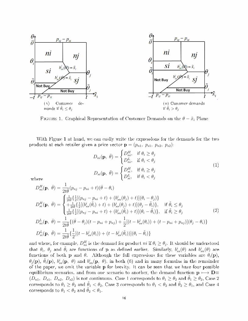
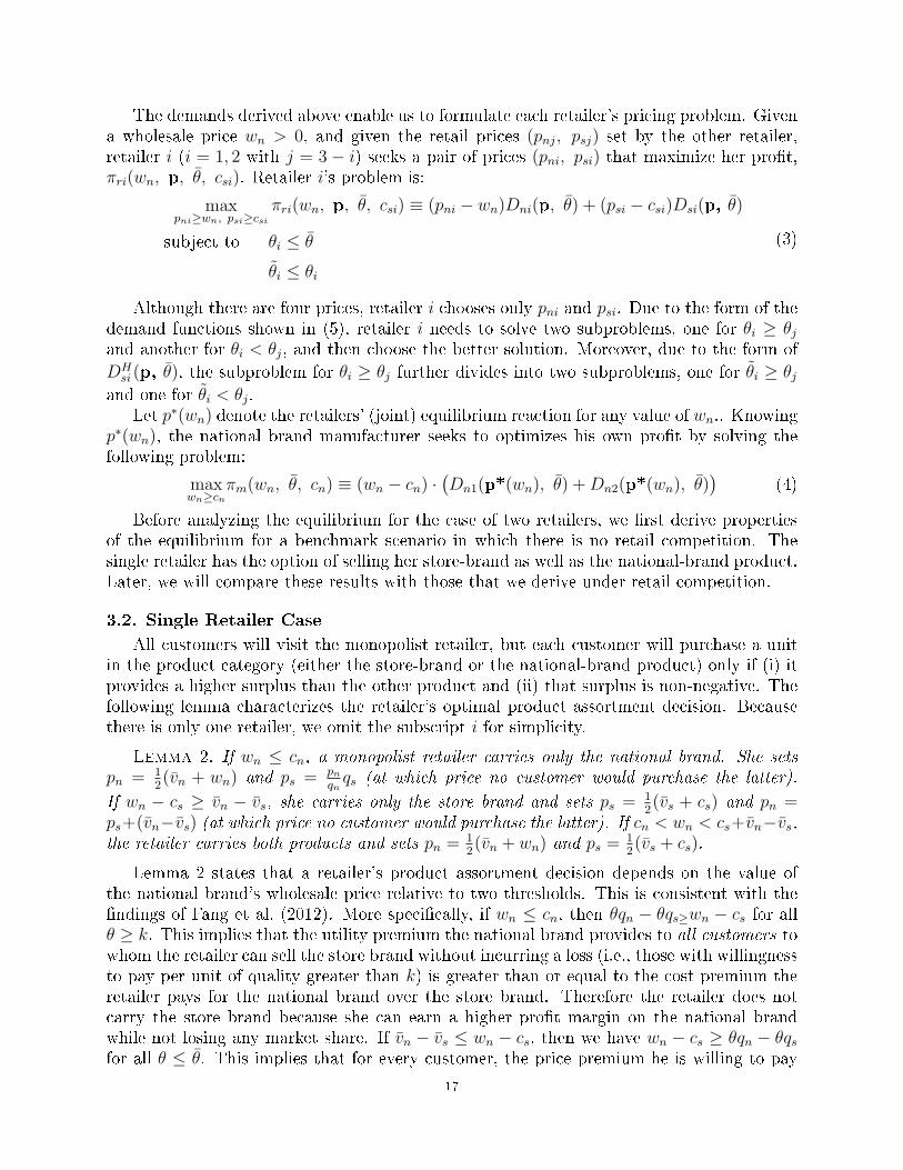
Figure 1 shows the partitioning of customer demand graphically on the θ − xi plane.Here, without loss of generality, we assume θi > θj (i = 1 or 2 and j = 3 − i). Under this

assumption, we need to divide our analysis into two cases: θi ≤ θj (shown in Figure 1(A))

and θi > θj (shown in Figure 1(B)). Note that in Figure 1, although it is not explicitly

stated, θi, θj, θi and θj are not parameters, but depend upon the retailers' pricing decisions.Expressions for the functions bisn(·) and biss(·) also depend upon the pricing decisions. Also,for the diagrams in Figure 1, we are implicitly assuming that t ≥ max{|pn2 − pn1|, |ps2 −ps1|, |bisn(θj)|}, i.e., the degree of customer loyalty is not too low, which guarantees thatnone of the demand regions represented in the diagrams vanish. For now, we proceed withour analysis under this assumption about t, but address other cases later in this section.

15

(a) Customer de-

mands if θi ≤ θj

(b) Customer demands

if θi > θj

Figure 1. Graphical Representation of Customer Demands on the θ − xi Plane

With Figure 1 at hand, we can easily write the expressions for the demands for the twoproducts at each retailer given a price vector p = (pn1, ps1, pn2, ps2):

Dni(p, θ) =

{DH

ni, if θi ≥ θj

DLni, if θi < θj

Dsi(p, θ) =

{DH

si , if θi ≥ θj

DLsi, if θi < θj

(1)

where

DHni(p, θ) =

1

2tθ(pnj − pni + t)(θ − θi)

DHsi (p, θ) =

12tθ

{12[(pnj − pni + t) + (bisn(θj) + t)](θi − θj)}

+ 12tθ

{12[(biss(θi) + t) + (biss(θj) + t)](θj − θi)}, if θi ≤ θj

12tθ

{12[(pnj − pni + t) + (bisn(θi) + t)](θi − θi)}, if θi ≥ θj

DLni(p, θ) =

1

2tθ{(θ − θj)(t− pni + pnj) +

1

2[(t− bjss(θi)) + (t− pni + pnj)](θj − θi)}

DLsi(p, θ) =

1

2tθ{12[(t− bjss(θi)) + (t− bjss(θi))](θi − θi)}

(2)

and where, for example, DHni is the demand for product ni if θi ≥ θj. It should be understood

that θi, θj and θi are functions of p as de�ned earlier. Similarly, biss(θ) and bisn(θ) arefunctions of both p and θ. Although the full expressions for these variables are θi(p),

θj(p), θi(p), biss(p, θ) and bisn(p, θ), in both (6) and in many formulas in the remainder

of the paper, we omit the variable p for brevity. It can be seen that we have four possibleequilibrium scenarios, and from one scenario to another, the demand function p 7−→ D≡(Dn1, Ds1, Dn2, Ds2) is not continuous. Case 1 corresponds to θ1 ≥ θ2 and θ1 ≥ θ2, Case 2

corresponds to θ1 ≥ θ2 and θ1 < θ2, Case 3 corresponds to θ1 < θ2 and θ2 ≥ θ1, and Case 4corresponds to θ1 < θ2 and θ2 < θ1.

16

The demands derived above enable us to formulate each retailer's pricing problem. Givena wholesale price wn > 0, and given the retail prices (pnj, psj) set by the other retailer,retailer i (i = 1, 2 with j = 3 − i) seeks a pair of prices (pni, psi) that maximize her pro�t,πri(wn, p, θ, csi). Retailer i's problem is:

maxpni≥wn, psi≥csi

πri(wn, p, θ, csi) ≡ (pni − wn)Dni(p, θ) + (psi − csi)Dsi(p, θ)

subject to θi ≤ θ

θi ≤ θi

(3)

Although there are four prices, retailer i chooses only pni and psi. Due to the form of thedemand functions shown in (5), retailer i needs to solve two subproblems, one for θi ≥ θjand another for θi < θj, and then choose the better solution. Moreover, due to the form of

DHsi (p, θ), the subproblem for θi ≥ θj further divides into two subproblems, one for θi ≥ θj

and one for θi < θj.Let p∗(wn) denote the retailers' (joint) equilibrium reaction for any value of wn.. Knowing

p∗(wn), the national brand manufacturer seeks to optimizes his own pro�t by solving thefollowing problem:

maxwn≥cn

πm(wn, θ, cn) ≡ (wn − cn) ·(Dn1(p*(wn), θ) +Dn2(p*(wn), θ)

)(4)

Before analyzing the equilibrium for the case of two retailers, we �rst derive propertiesof the equilibrium for a benchmark scenario in which there is no retail competition. Thesingle retailer has the option of selling her store-brand as well as the national-brand product.Later, we will compare these results with those that we derive under retail competition.

3.2. Single Retailer Case

All customers will visit the monopolist retailer, but each customer will purchase a unitin the product category (either the store-brand or the national-brand product) only if (i) itprovides a higher surplus than the other product and (ii) that surplus is non-negative. Thefollowing lemma characterizes the retailer's optimal product assortment decision. Becausethere is only one retailer, we omit the subscript i for simplicity.

Lemma 2. If wn ≤ cn, a monopolist retailer carries only the national brand. She setspn = 1

2(vn + wn) and ps = pn

qnqs (at which price no customer would purchase the latter).

If wn − cs ≥ vn − vs, she carries only the store brand and sets ps = 12(vs + cs) and pn =

ps+(vn−vs) (at which price no customer would purchase the latter). If cn < wn < cs+vn−vs,the retailer carries both products and sets pn = 1

2(vn + wn) and ps =

12(vs + cs).

Lemma 2 states that a retailer's product assortment decision depends on the value ofthe national brand's wholesale price relative to two thresholds. This is consistent with the�ndings of Fang et al. (2012). More speci�cally, if wn ≤ cn, then θqn − θqs≥wn − cs for allθ ≥ k. This implies that the utility premium the national brand provides to all customers towhom the retailer can sell the store brand without incurring a loss (i.e., those with willingnessto pay per unit of quality greater than k) is greater than or equal to the cost premium theretailer pays for the national brand over the store brand. Therefore the retailer does notcarry the store brand because she can earn a higher pro�t margin on the national brandwhile not losing any market share. If vn − vs ≤ wn − cs, then we have wn − cs ≥ θqn − θqsfor all θ ≤ θ. This implies that for every customer, the price premium he is willing to pay

17

for the national brand over the store brand is less than the cost premium the retailer incursby selling a unit of the national brand instead of the store brand. Therefore the retailercompletely forgoes the national-brand product.

If the wholesale price falls between cn and cs + vn − vs, it is more pro�table for theretailer to sell the national brand to the subset of customers who have a willingness to payper unit of quality above a threshold and the store brand to the remaining customers, sothe retailer carries both products. In this case, the retailer sets the retail prices in the sameway as if each product were the sole product she carries. That is, she sets the price of thenational (store) brand as half the sum of its procurement cost and the highest valuation for

the national (store) brand among customers. As the wholesale price increases, θ = ps/qs (setby the retailer implicitly via her choice of ps) stays the same whereas θ = (pn− ps)/(qn− qs)increases, leading to more store brand sales and fewer national brand sales while the totalsales stays the same.

We characterize the manufacturer's equilibrium strategy and other equilibrium outcomesunder this benchmark scenario in the following lemma.

Lemma 3. In a market with a monopolist retailer who has the option to o�er a storebrand, the equilibrium wholesale price is wn = 1

2(vn + cn) − 1

2(vs − cs). In response, the

retailer carries both products and sets prices according to Lemma 2. The resulting customerdemands are Dn = θ′

4θfor the national brand and Ds =

θ′

2θfor the store brand, and the pro�ts

of the manufacturer and the retailer are, respectively, πm = θ′

8θ[(vn − cn)− (vs − cs)] and

πr =θ′

16θ[(vn − cn) + 5(vs − cs)].

4. Assortment and Pricing under Retail Competition

The focus of this section is on the retailers' optimal assortment and pricing strategiesfor a given national brand wholesale price. In Section 4.1, we derive the equilibrium andin Section 4.2, we study how the equilibrium prices and pro�ts change with the level ofcustomer loyalty.

4.1. Retailers' Product Assortment and Pricing

To simplify the analysis and for ease of exposition, we assume that for both retailers,their respective pro�t functions are quasi-concave in their prices, subject to certain con-ditions that we will explain later in this section. This is a common assumption and issupported by our observations from numerical examples. Given this, from results in gametheory (see, for example, Osborne and Rubinstein (1994)) we know that a pure-strategy Nashequilibrium exists for the pricing game between the retailers. We now proceed to study itscharacteristics. The traditional approach to �nd a price equilibrium between two retailersis to (1) solve for the explicit expressions characterizing each retailer's best responses and(2) solve for the crossing points of the retailers' best responses and express them as explicitfunctions of wn. However, in our model, the demand functions are discontinuous and non-linear in the price variables (see the discussion in Section 3.2). Indeed, it is impossible toobtain explicit expressions for retailers' price responses and the equilibrium prices. We thustake an alternate approach: we derive and analyze the �rst-order-conditions for each re-tailer's pro�t-maximization problem to characterize the retailers' optimal strategies withoutexplicitly solving the �rst-order-conditions. Details can be found in Appendix D. Here, we

18

summarize the main results. We start by presenting each retailer's optimal product assort-ment strategy given any pricing and assortment strategy taken by the other retailer. Thisresult facilitates our proof (presented later) of the uniqueness of the equilibrium.

proposition 1. Each retailer's best response in terms of product assortment, givenany strategy taken by the other retailer, is to carry only the national brand if wn ≤ cn, tocarry only the store brand if wn ≥ csi + (vn − vsi), and to carry both products otherwise.

Proposition 1 implies that, under retail competition, for any given wholesale price, eachretailer makes the product assortment decision in the same way as if she were a downstreammonopolist. This result is certainly not intuitive. It implies that that a retailer's optimalproduct assortment decision is not a�ected by the existence of the other retailer, nor is ita�ected by the assortment or pricing decisions of the other retailer. Intuitively, we wouldimagine in a Nash game between the two retailers, one retailer's best response depends uponthe strategy of the other retailer. But Proposition 1 says this is not so, which is quitesurprising.

So what is the intuition behind Proposition 1? If it is less pro�table for a retailer to sellone product (versus the other) to all customers, the retailer will not carry the less pro�tableproduct at all. For example, if wn ≥ cs+(vn−vsi), the per-unit cost premium retailer i incursfrom selling the national brand (versus the store brand) is greater then the maximum per-unit price premium consumers are willing to pay. Thus, it is not worthwhile for the retailerto carry the national brand at all. This comparison between the two products remains thesame whether a retailer is a monopolist or is facing competition. We will see later, however,that the national brand manufacturer takes into account the retailers' reactions (includingthe assortment decisions) when choosing the wholesale price, so the introduction of retailcompetition may ultimately a�ect retailers' assortment decisions. We study this issue in thenext section.

Next, we establish the uniqueness of the equilibrium.

proposition 2. There exists a t0 with 0 < t0 < +∞ such that, whenever t > t0, theprice equilibrium between retailer is unique for all wn.

In Appendix E, we prove the result for values of t for which the demand segmentationdiagram has the form of Figure 1(A) or (B). As the value of t declines, the right and leftboundaries in Figure 1(B) move inward, as shown by the dashed lines in Figure 2(A). Theresulting extracted diagram is shown in Figure 2(B). Then �nally, as t becomes very small,the demand segmentation approaches the form shown in Figure 2(C): the diagonal lines�atten out and become horizontal at t = 0. When this happens, each retailer is able to seizea large share of the national brand demand from the other retailer by reducing the priceof the national brand slightly. As a result, at equilibrium each retailer sets the nationalbrand price at the wholesale price and gains pro�t exclusively from her store brand. Theequilibrium is also unique for 0 ≤ t ≤ t0 (i.e., for the demand segmentation diagrams shownin Figures 2(B) and 2(C)) but we have omitted the proofs for the sake of brevity.

How do the prices a retailer sets when facing competition compare to those she wouldset as a monopolist, and how do the respective demands compare? We answer this questionby �rst introducing the following proposition, in which θmi and θmi denote the optimal values

of θ and θ, respectively, that retailer i would set when she is a downstream monopolist (cf.Lemma 3).

19

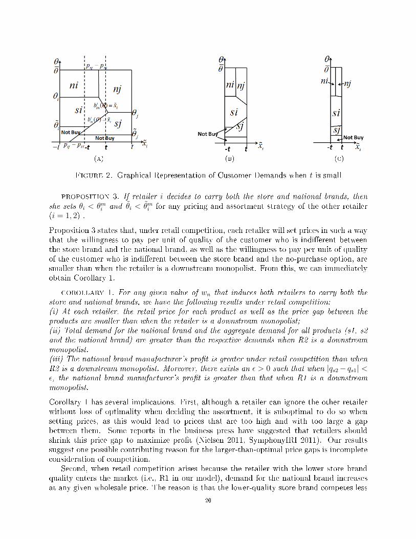
(a) (b) (c)

Figure 2. Graphical Representation of Customer Demands when t is small

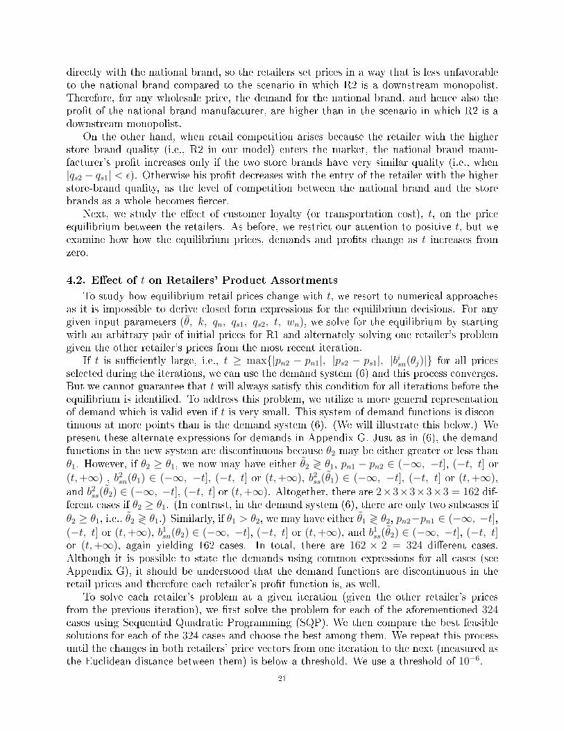
proposition 3. If retailer i decides to carry both the store and national brands, thenshe sets θi < θmi and θi < θmi for any pricing and assortment strategy of the other retailer(i = 1, 2) .

Proposition 3 states that, under retail competition, each retailer will set prices in such a waythat the willingness to pay per unit of quality of the customer who is indi�erent betweenthe store brand and the national brand, as well as the willingness to pay per unit of qualityof the customer who is indi�erent between the store brand and the no-purchase option, aresmaller than when the retailer is a downstream monopolist. From this, we can immediatelyobtain Corollary 1.

corollary 1. For any given value of wn that induces both retailers to carry both thestore and national brands, we have the following results under retail competition:(i) At each retailer, the retail price for each product as well as the price gap between theproducts are smaller than when the retailer is a downstream monopolist;(ii) Total demand for the national brand and the aggregate demand for all products (s1, s2and the national brand) are greater than the respective demands when R2 is a downstreammonopolist.(iii) The national brand manufacturer's pro�t is greater under retail competition than whenR2 is a downstream monopolist. Moreover, there exists an ϵ > 0 such that when |qs2− qs1| <ϵ, the national brand manufacturer's pro�t is greater than that when R1 is a downstreammonopolist.

Corollary 1 has several implications. First, although a retailer can ignore the other retailerwithout loss of optimality when deciding the assortment, it is suboptimal to do so whensetting prices, as this would lead to prices that are too high and with too large a gapbetween them. Some reports in the business press have suggested that retailers shouldshrink this price gap to maximize pro�t (Nielsen 2011, SymphonyIRI 2011). Our resultssuggest one possible contributing reason for the larger-than-optimal price gaps is incompleteconsideration of competition.

Second, when retail competition arises because the retailer with the lower store brandquality enters the market (i.e., R1 in our model), demand for the national brand increasesat any given wholesale price. The reason is that the lower-quality store brand competes less

20

directly with the national brand, so the retailers set prices in a way that is less unfavorableto the national brand compared to the scenario in which R2 is a downstream monopolist.Therefore, for any wholesale price, the demand for the national brand, and hence also thepro�t of the national brand manufacturer, are higher than in the scenario in which R2 is adownstream monopolist.

On the other hand, when retail competition arises because the retailer with the higherstore brand quality (i.e., R2 in our model) enters the market, the national brand manu-facturer's pro�t increases only if the two store brands have very similar quality (i.e., when|qs2 − qs1| < ϵ). Otherwise his pro�t decreases with the entry of the retailer with the higherstore-brand quality, as the level of competition between the national brand and the storebrands as a whole becomes �ercer.

Next, we study the e�ect of customer loyalty (or transportation cost), t, on the priceequilibrium between the retailers. As before, we restrict our attention to positive t, but weexamine how how the equilibrium prices, demands and pro�ts change as t increases fromzero.

4.2. E�ect of t on Retailers' Product Assortments

To study how equilibrium retail prices change with t, we resort to numerical approachesas it is impossible to derive closed form expressions for the equilibrium decisions. For anygiven input parameters (θ, k, qn, qs1, qs2, t, wn), we solve for the equilibrium by startingwith an arbitrary pair of initial prices for R1 and alternately solving one retailer's problemgiven the other retailer's prices from the most recent iteration.

If t is su�ciently large, i.e., t ≥ max{|pn2 − pn1|, |ps2 − ps1|, |bisn(θj)|} for all pricesselected during the iterations, we can use the demand system (6) and this process converges.But we cannot guarantee that t will always satisfy this condition for all iterations before theequilibrium is identi�ed. To address this problem, we utilize a more general representationof demand which is valid even if t is very small. This system of demand functions is discon-tinuous at more points than is the demand system (6). (We will illustrate this below.) Wepresent these alternate expressions for demands in Appendix G. Just as in (6), the demandfunctions in the new system are discontinuous because θ2 may be either greater or less thanθ1. However, if θ2 ≥ θ1, we now may have either θ2 ≷ θ1, pn1 − pn2 ∈ (−∞, −t], (−t, t] or

(t,+∞) , b2sn(θ1) ∈ (−∞, −t], (−t, t] or (t,+∞), b2ss(θ1) ∈ (−∞, −t], (−t, t] or (t,+∞),

and b2ss(θ2) ∈ (−∞, −t], (−t, t] or (t,+∞). Altogether, there are 2×3×3×3×3 = 162 dif-ferent cases if θ2 ≥ θ1. (In contrast, in the demand system (6), there are only two subcases if

θ2 ≥ θ1, i.e., θ2 ≷ θ1.) Similarly, if θ1 > θ2, we may have either θ1 ≷ θ2, pn2−pn1 ∈ (−∞, −t],

(−t, t] or (t,+∞), b1sn(θ2) ∈ (−∞, −t], (−t, t] or (t,+∞), and b1ss(θ2) ∈ (−∞, −t], (−t, t]or (t,+∞), again yielding 162 cases. In total, there are 162 × 2 = 324 di�erent cases.Although it is possible to state the demands using common expressions for all cases (seeAppendix G), it should be understood that the demand functions are discontinuous in theretail prices and therefore each retailer's pro�t function is, as well.

To solve each retailer's problem at a given iteration (given the other retailer's pricesfrom the previous iteration), we �rst solve the problem for each of the aforementioned 324cases using Sequential Quadratic Programming (SQP). We then compare the best feasiblesolutions for each of the 324 cases and choose the best among them. We repeat this processuntil the changes in both retailers' price vectors from one iteration to the next (measured asthe Euclidean distance between them) is below a threshold. We use a threshold of 10−6.

21

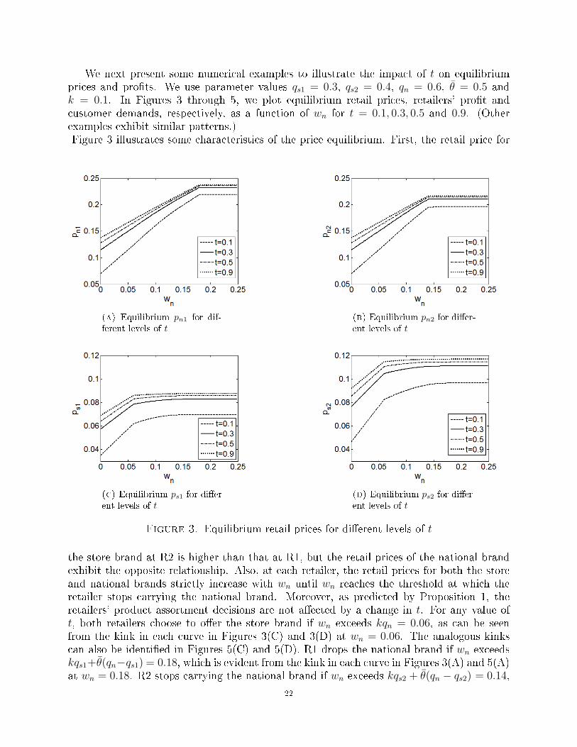
We next present some numerical examples to illustrate the impact of t on equilibriumprices and pro�ts. We use parameter values qs1 = 0.3, qs2 = 0.4, qn = 0.6, θ = 0.5 andk = 0.1. In Figures 3 through 5, we plot equilibrium retail prices, retailers' pro�t andcustomer demands, respectively, as a function of wn for t = 0.1, 0.3, 0.5 and 0.9. (Otherexamples exhibit similar patterns.)Figure 3 illustrates some characteristics of the price equilibrium. First, the retail price for

(a) Equilibrium pn1 for dif-ferent levels of t

(b) Equilibrium pn2 for di�er-ent levels of t

(c) Equilibrium ps1 for di�er-ent levels of t

(d) Equilibrium ps2 for di�er-ent levels of t

Figure 3. Equilibrium retail prices for di�erent levels of t

the store brand at R2 is higher than that at R1, but the retail prices of the national brandexhibit the opposite relationship. Also, at each retailer, the retail prices for both the storeand national brands strictly increase with wn until wn reaches the threshold at which theretailer stops carrying the national brand. Moreover, as predicted by Proposition 1, theretailers' product assortment decisions are not a�ected by a change in t. For any value oft, both retailers choose to o�er the store brand if wn exceeds kqn = 0.06, as can be seenfrom the kink in each curve in Figures 3(C) and 3(D) at wn = 0.06. The analogous kinkscan also be identi�ed in Figures 5(C) and 5(D). R1 drops the national brand if wn exceedskqs1+θ(qn−qs1) = 0.18, which is evident from the kink in each curve in Figures 3(A) and 5(A)at wn = 0.18. R2 stops carrying the national brand if wn exceeds kqs2 + θ(qn − qs2) = 0.14,

22

as can be identi�ed from the kinks in the curves in Figures 3(B) and 5(B) at wn = 0.14.These thresholds do not vary with the value of t. However, all of the retail prices increasewith t, as expected, due to reduced competition.

(a) Equilibrium πr1 for dif-ferent levels of t

(b) Equilibrium πr2 for di�er-ent levels of t

Figure 4. Retailers' pro�t for di�erent levels of t

The retailers' pro�ts for di�erent values of t are shown in Figure 4. Comparing Figures4(A) and 4(B), it can be seen that the pro�ts of the two retailers are equal and both aredecreasing with wn for wn ≤ 0.06 (that is, when both of them carry only the national brand).For wn > 0.06, R1's pro�t is smaller than that of R2. R1's pro�t keeps decreasing with wn

until the retailer stops carrying the national brand (at about wn = 0.18). In comparison,R2's pro�t �rst decreases and then increases with wn until both retailers stop carrying thenational brand. The fact that R2's pro�t increases with wn for a range of wn is quitecounterintuitive, as one would conjecture that both retailers should become worse o� as wn

increases. What is happening here is the following: as wn increases in this range, R2 pricesso as to sell greater quantities of her store brand. This not only shields her from the decliningmargin on the national brand as wn increases, but also lessens the degree of competition shefaces from R1. As a result, R2 may be better o� as wn increases in this range. Note thatthis would never happen if R2 were a downstream monopolist. Finally, as t increases, bothretailers' pro�ts increase for all values of wn as the level of retail competition declines.

Figure 5 shows the customer demands at the equilibrium prices for di�erent values oft. The national brand demand at each retailer strictly decreases with wn before it reacheszero, as expected. The store brand demand at each retailer increases with wn for the intervalof wn in which the retailer carries both products. Also, as t increases, the demands for allproducts decline due to lessened competition which drives up retail prices, which in turndrives down customer demands.

5. Manufacturer's Strategy under Retail Competition

In this section, we investigate the manufacturer's strategy regarding the breadth of prod-uct distribution, i.e., whether to distribute through both retailers or only one. Due to thestructure of each retailer's product assortment strategy (see Proposition 1), the nationalbrand manufacturer can either sell through both retailers by setting the wholesale price in

23

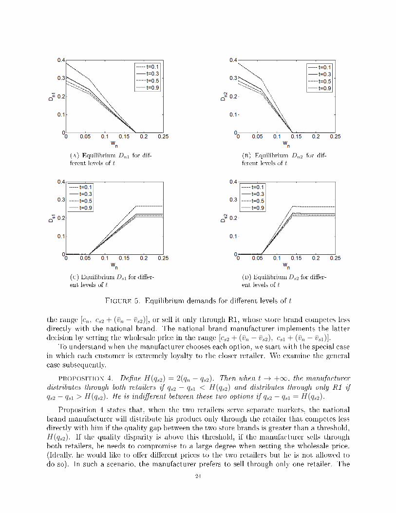
(a) Equilibrium Dn1 for dif-ferent levels of t

(b) Equilibrium Dn2 for dif-ferent levels of t

(c) EquilibriumDs1 for di�er-ent levels of t

(d) EquilibriumDs2 for di�er-ent levels of t

Figure 5. Equilibrium demands for di�erent levels of t

the range [cn, cs2 + (vn − vs2)], or sell it only through R1, whose store brand competes lessdirectly with the national brand. The national brand manufacturer implements the latterdecision by setting the wholesale price in the range [cs2 + (vn − vs2), cs1 + (vn − vs1)].

To understand when the manufacturer chooses each option, we start with the special casein which each customer is extremely loyalty to the closer retailer. We examine the generalcase subsequently.

proposition 4. De�ne H(qs2) = 2(qn − qs2). Then when t → +∞, the manufacturerdistributes through both retailers if qs2 − qs1 < H(qs2) and distributes through only R1 ifqs2 − qs1 > H(qs2). He is indi�erent between these two options if qs2 − qs1 = H(qs2).

Proposition 4 states that, when the two retailers serve separate markets, the nationalbrand manufacturer will distribute his product only through the retailer that competes lessdirectly with him if the quality gap between the two store brands is greater than a threshold,H(qs2). If the quality disparity is above this threshold, if the manufacturer sells throughboth retailers, he needs to compromise to a large degree when setting the wholesale price.(Ideally, he would like to o�er di�erent prices to the two retailers but he is not allowed todo so). In such a scenario, the manufacturer prefers to sell through only one retailer. The

24

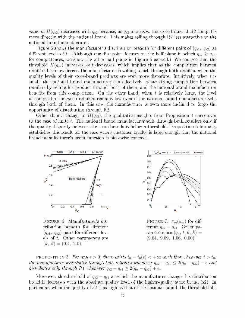
value of H(qs2) decreases with qs2 because, as qs2 increases, the store brand at R2 competesmore directly with the national brand. This makes selling through R2 less attractive to thenational brand manufacturer.

Figure 6 shows the manufacturer's distribution breadth for di�erent pairs of (qs1, qs2) atdi�erent levels of t. (Although our discussion focuses on the half plane in which qs2 ≥ qs1,for completeness, we show the other half plane in Figure 6 as well.) We can see that thethreshold H(qs2) increases as t decreases, which implies that as the competition betweenretailers becomes �ercer, the manufacturer is willing to sell through both retailers when thequality levels of their store-brand products are even more disparate. Intuitively, when t issmall, the national brand manufacturer can e�ectively create strong competition betweenretailers by selling his product through both of them, and the national brand manufacturerbene�ts from this competition. On the other hand, when t is relatively large, the levelof competition between retailers remains low even if the national brand manufacturer sellsthrough both of them. In this case the manufacturer is even more inclined to forgo theopportunity of distributing through R2.

Other than a change in H(qs2), the qualitative insights from Proposition 4 carry overto the case of �nite t. The national brand manufacturer sells through both retailers only ifthe quality disparity between the store brands is below a threshold. Proposition 5 formallyestablishes this result for the case where customer loyalty is large enough that the nationalbrand manufacturer's pro�t function is piecewise concave.

Figure 6. Manufacturer's dis-tribution breadth for di�erent(qs1, qs2) pairs for di�erent lev-els of t. Other parameters are(k, θ) = (0.4, 2.0).

Figure 7. πm(wn) for dif-ferent qs2 − qs1. Other pa-rameters are (qn, t, θ, k) =(9.64, 9.09, 1.06, 0.00).

proposition 5. For any ϵ > 0, there exists t0 = t0(ϵ) < +∞ such that whenever t > t0,the manufacturer distributes through both retailers whenever qs2 − qs1 ≤ 2(qn − qs2)− ϵ anddistributes only through R1 whenever qs2 − qs1 ≥ 2(qn − qs2) + ϵ.

Moreover, the threshold of qs2 − qs1 at which the manufacturer changes his distributionbreadth decreases with the absolute quality level of the higher-quality store brand (s2). Inparticular, when the quality of s2 is as high as that of the national brand, the threshold falls

25

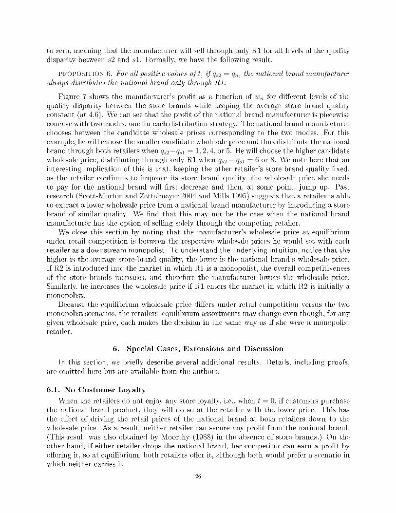
to zero, meaning that the manufacturer will sell through only R1 for all levels of the qualitydisparity between s2 and s1. Formally, we have the following result.

proposition 6. For all positive values of t, if qs2 = qn, the national brand manufactureralways distributes the national brand only through R1.

Figure 7 shows the manufacturer's pro�t as a function of wn for di�erent levels of thequality disparity between the store brands while keeping the average store brand qualityconstant (at 4.6). We can see that the pro�t of the national brand manufacturer is piecewiseconcave with two modes, one for each distribution strategy. The national brand manufacturerchooses between the candidate wholesale prices corresponding to the two modes. For thisexample, he will choose the smaller candidate wholesale price and thus distribute the nationalbrand through both retailers when qs2−qs1 = 1, 2, 4, or 5. He will choose the higher candidatewholesale price, distributing through only R1 when qs2 − qs1 = 6 or 8. We note here that aninteresting implication of this is that, keeping the other retailer's store brand quality �xed,as the retailer continues to improve its store brand quality, the wholesale price she needsto pay for the national brand will �rst decrease and then, at some point, jump up. Pastresearch (Scott-Morton and Zettelmeyer 2004 and Mills 1995) suggests that a retailer is ableto extract a lower wholesale price from a national brand manufacturer by introducing a storebrand of similar quality. We �nd that this may not be the case when the national brandmanufacturer has the option of selling solely through the competing retailer.

We close this section by noting that the manufacturer's wholesale price at equilibriumunder retail competition is between the respective wholesale prices he would set with eachretailer as a downstream monopolist. To understand the underlying intuition, notice that thehigher is the average store-brand quality, the lower is the national brand's wholesale price.If R2 is introduced into the market in which R1 is a monopolist, the overall competitivenessof the store brands increases, and therefore the manufacturer lowers the wholesale price.Similarly, he increases the wholesale price if R1 enters the market in which R2 is initially amonopolist.

Because the equilibrium wholesale price di�ers under retail competition versus the twomonopolist scenarios, the retailers' equilibrium assortments may change even though, for anygiven wholesale price, each makes the decision in the same way as if she were a monopolistretailer.

6. Special Cases, Extensions and Discussion

In this section, we brie�y describe several additional results. Details, including proofs,are omitted here but are available from the authors.

6.1. No Customer Loyalty

When the retailers do not enjoy any store loyalty, i.e., when t = 0, if customers purchasethe national brand product, they will do so at the retailer with the lower price. This hasthe e�ect of driving the retail prices of the national brand at both retailers down to thewholesale price. As a result, neither retailer can secure any pro�t from the national brand.(This result was also obtained by Moorthy (1988) in the absence of store brands.) On theother hand, if either retailer drops the national brand, her competitor can earn a pro�t byo�ering it, so at equilibrium, both retailers o�er it, although both would prefer a scenario inwhich neither carries it.

26

With the national brand providing no pro�t, the store brands are the sole source of pro�tand the sole means by which the retailers are able to di�erentiate themselves. In practice,major retailers almost always enjoy some level of customer loyalty. Therefore we rarely seeretailers getting no margins from national brands. However, for retailers facing strong head-to-head competition, this result implies that the markup on national brands can be fairlylow and that retailers are essentially deriving most of their pro�t from store brands. Indeed,there is empirical evidence showing that some major retailers set high markup ratios on storebrands, while at the same time their markup ratios for national brands are close to 1 (seeBarsky et al. 2003). Although there may be other explanations for this phenomenon (forexample, di�erences in marginal costs for the products), it is consistent with our �ndings.Thus, retail competition could be one factor that leads to low markup ratios on nationalbrands compared to those on store brands.

We conclude that when retailers compete head-to-head, the structure of retailers' prod-uct assortment and pricing di�ers from when each enjoys some degree of customer loyalty.Therefore, for the sake of answering the questions raised in Section 1, it is important toinclude a positive parameter t in our model to capture reality.

6.2. Production Cost

Thus far, we have assumed that both retailers and the manufacturer share the sameproduction cost function, i.e., c = kq. If one retailer has a cost advantage over the other,we can let k1 = k2. Without loss of generality, we assume ki < kj (i ∈ {1, 2} and j =3− i). In this scenario, the retailers' product assortment strategy can be characterized as ageneralization of Proposition 2:

corollary 2. If csi = kiqsi for i = 1, 2 and k1 = k2, each retailer's best response interms of product assortment is to carry only the national brand if wn ≤ kiqn, to carry onlythe store brand if wn ≥ csi + (vn − vsi), and to carry both products otherwise.

Recall that when the retailers have the same production cost parameters, the lowernational brand wholesale price threshold (above which the retailers choose to carry a storebrand) coincide with each other. This no longer holds if their production cost parametersdi�er. Retailer i (i.e., the retailer with the smaller cost parameter) starts to carry the storebrand at a lower wholesale price than the other retailer. When wn ∈ (kiqn, kjqn], retaileri carries both the national and the store brand and retailer j carries the national brandonly. This phenomenon has additional implications for the national brand manufacturer'sstrategy, as we delineate below.Case (1): k ≥ max{k1, k2}. In this case, the national brand manufacturer never sets thewholesale price such that one or both retailer(s) only carry the national brand product.Therefore, just as in our basic model, he chooses between two candidate wholesale prices,which is equivalent to choosing between distributing the national-brand product throughone or both retailers. At either candidate wholesale price, both retailers will carry theirrespective store brand.Case (2): ki < k < kj. In this case, the national brand manufacturer chooses among threecandidate wholesale prices, each corresponding to a di�erent distribution strategy: sellingthrough both retailers while foreclosing the store brand at retailer j , selling through bothretailers but foreclosing neither of the store brands, and selling through only the retailerwith the lower-quality store brand while not foreclosing her store brand.

27

Case (3): k < ki < kj. In this case, the national brand manufacturer chooses amongfour candidate wholesale prices, each corresponding to a di�erent distribution strategy. Onestrategy is selling through both retailers while foreclosing the store brand at both of them.The other three are the same as those mentioned above for the case of ki < k < kj.

Mills (1995, 1999) �nds that it is optimal for the national brand manufacturer to foreclosethe store brand if its quality falls into a particular range. We note here that this result iscontingent on his assumption that the national brand has an advantage in terms of cost-per-unit-of-quality (as in Case (2) or (3) above). If the national brand does not enjoy a costadvantage over either of the store brands (as in Case (1)), the national brand manufacturerwould never �nd it optimal to foreclose a store brand because he would need to set thewholesale price below his production cost to accomplish this. This e�ect has been found byFang et al. (2012) in the case of a single retailer. We have shown that it also applies whenwhen retail competition is introduced.

6.3. Heterogeneity in Transportation Costs

In our basic model, we have assumed that customers are uniformly distributed on aHotelling line between the retailers. Our model can be extended to capture heterogeneityin transportation costs by an appropriate placement of each customer on the Hotelling linebetween the two retailers and using a general distribution of customers along the Hotellingline. To implement this, one can use the demand expressions in Appendix G and thensubstitute a general distribution of customers' locations into the demand expressions. Theanalysis could then be conducted in a similar fashion. From numerical examples, we havefound that retailers' product assortment strategy (i.e., Proposition 1) and the manufacturer'sstrategy regarding distribution breath (i.e., distributing through both retailers only if thequality disparity between the two store brands is low) remain valid for common symmetricbell-shaped distributions of customers along the Hotelling line.

6.4. Market Share versus Pro�tability

In Section 5, we establish that it is sometimes pro�table for the manufacturer to sellthrough only one of retailers. In reality, however, national brand manufacturers may stillsell through both retailers to maintain market share even though they realize that doingso may have an adverse e�ect on pro�t. Indeed, national brand manufacturers are facinga tradeo� between market share and pro�tability when making the decision of whether tosell through a retailer with a very high quality store brand. For example, a senior managerof a large national brand revealed to us that he chooses to continue to sell through all themajor retailers although pro�t may su�er in the short run. Maintaining a large marketshare has bene�ts if it reduces competition in the long-run, but whether this actually occursis an ongoing topic of discussion in the literature. Many researchers have suggested thatincreasing market share at a cost may not prove to be pro�table in the long-term (Fruhan1972, Hamermesh et al. 1978, Woo and Cooper 1981). For example, Wernerfelt (1986)showed that �rms do well by attacking in the early stages of the product life cycle but arebetter o� not overplaying their cards in the stable periods of the life cycle.

28

7. Conclusions

In this paper, we study a retailer's product assortment and pricing problem when she hasthe option to carry a store brand, a national brand, or both. We �rst derive the structure ofthe retailer's optimal assortment and prices in two settings: (1) when she is a downstreammonopolist and (2) when she faces competition from another retailer who may also o�er thesame national brand and a competing store brand. Past research has established that storebrands help generate store tra�c and help a store better di�erentiate itself. As a result, onewould expect that a retailer would be more likely to introduce a store brand as a competitivestrategy when she faces retail competition. In contrast, we �nd that in the presence of retailcompetition, for any given wholesale price of the national brand product, a retailer makesthe product assortment decision in the same way as if she were a downstream monopolist.The underlying reason for this result is that a retailer's assortment decision is determinedby a comparison between the pro�tability of her store and national brands, which does notinvolve the other retailer. However, the presence of multiple retailers a�ects the nationalbrand manufacturer's choice of a wholesale price, which then a�ects the ultimate assortmentsand prices at the retail level.

We also characterize how each retailer's optimal assortment decision depends on thenational brand's wholesale price. For wholesale prices below a lower threshold, the retailercarries only the national brand and for wholesale prices above an upper threshold, the retailercarries only the store brand. For wholesale prices between the lower and upper thresholds,the retailer carries both brands. The thresholds may, in general, di�er by retailer, but if theproduction cost per unit of quality is the same for both retailers, then the lower thresholdsare the same for both retailers. Although a retailer in a duopoly is able to make the optimalassortment decision in the same way as if she were a monopolist, she needs to take intoaccount retail prices set by her competitor to set the optimal retail prices. Failing to do somay have a sizable e�ect on pro�ts.

Not surprisingly, the equilibrium retail prices of all o�ered products decline with theintroduction of retail competition, but interestingly, the optimal gap between the prices ofthe store and national brands also decline. Thus, the introduction of retail competition putsgreater pressure on the retail price of the national brand than it does on the retail prices ofthe store brands. Several news reports and market research suggest that the retailers areessentially �leaving money on the table� by setting store-brand prices too low. (See, e.g.,Kumar and Steenkamp 2007).

We also study the national brand manufacturer's optimal pricing decision which a�ectsthe retailers' product assortments. From our characterization of how each retailer's assort-ment changes as a function of the wholesale price, we can infer that the national brandmanufacturer needs to choose between two regimes: (1) selling through both retailers andoptimizing the wholesale price within the interval in which both retailers choose to o�er thenational brand (along with their respective store brand), and (2) selling through only theretailer with the lower-quality store brand and optimizing the wholesale price within therelevant price interval.

Our results suggest that the manufacturer should sell his national brand through onlyone retailer if the quality disparity between the two store brands exceeds a threshold. Witha large quality disparity, the manufacturer would charge the retailers di�erent wholesaleprices if he were allowed to do so. He would need to compromise a lot when setting a singlewholesale price, so he may be better o� distributing through one retailer.

29

We also study the e�ect of customer loyalty. When there is no customer loyalty, bothretailers stop carrying the national brand when the wholesale price exceeds the same thresh-old. Thus, the national brand manufacturer always distributes through both retailers. Theretailers end up in a prisoner's dilemma at the equilibrium: both of them could have earneda higher pro�t if neither of them had carried the national brand, but they both end upcarrying it. As the degree of customer loyalty increases, the national brand manufacturermay or may not distribute through both retailers depending upon the quality levels of thetwo store-brand products, as discussed above.

As discussed, our model can be extended to handle di�erent production cost functions(as a function of quality) for the various products as well as heterogeneity in customer loyaltyto the retailers.

In this paper, we assume that store-brand quality levels are exogenous and that theretailers already o�er or are ready to o�er their respective store brands. Further research isneeded to determine how a retailer should choose the quality of a new store brand when facingcompetition from a retailer that has, or can o�er, her own store brand, along with the nationalbrand. We are pursuing research along these lines. Further research is also needed to studyretail competition in settings in which the manufacturers of the store-brand products�bothnational brand manufacturers and third-party producers�are strategic players. For thesesettings, equilibria are much more di�cult to derive because there will be four or more partiesin the competitive game.

APPENDICES

Appendix A: Proof of Lemma 1

If any of the relations in (i) or (ii) fails to hold for retailer i at the equilibrium, she coulddecrease one of the retail prices without a�ecting either her own pro�t or the pricing decisionsof the other retailer. Then given Assumption 1, she will decrease the relevant price.

Appendix B: Transformed Problems

In this Appendix, we establish the equivalence of a market with parameters (θ, k) and atransformed market with parameters (θ′, 0). De�ne p′ ≡ (p′n1, p

′s1, p

′n2, p

′s2) ≡ p− c where

c ≡ (cn, cs1, cn, cs2), w′n ≡ wn−cn, θ

′ ≡ θ−k , θ′i ≡ θi−k (=p′ni−p′siqn−qsi

) and θ′i = θi−k (=p′siqni

)for i = 1, 2. Then we have the following lemma, which can be obtained from straightforwardalgebraic manipulations.

Lemma 4. Dni(p, θ) =θ′

θDni(p

′, θ′). Moreover, πri(wn,p, θ, csi) =θ′

θπri(w

′n,p

′, θ′, 0) and

πm(wn, θ, cn) =θ′

θπm(w

′n, θ

′, 0).

As such, if the equilibrium prices for the transformed market are (w′n, p

′(w′n)), we can

immediately write the equilibrium prices of the original market as (w′n + cn, p

′(w′n) + c).

As such, here and throughout the remaining Appendices, we will only present proofs ofthe lemmas and propositions for a market with parameters (θ, 0) and omit the proofs forthe original markets (i.e., the markets with parameters (θ, k)). Nevertheless, the resultsimmediately generalize with appropriate transformations of the prices.

30

Appendix C: Proofs of Lemmas 2 and 3

The customer demands under this scenario are Dn(p, θ) = 1θ(θ − pn−ps

qn−qs) and Ds(p, θ) =

1θ(pn−psqn−qs

− psqs). It is easy to con�rm that πr(wn, p, θ, 0) is concave in the retail prices.

Setting the �rst derivatives of maxp=(pn,ps)≥0

πr(wn, p, θ, 0) with respect to the prices equal to

zero, we obtain pn(wn) =12(θqn + wn) and ps(wn) =

12θqs. It remains to verify whether the

solution is an interior point in the region of (pn, ps) satisfying

θ >pn − psqn − qs

(5)

andpnqn

>psqs

(6)

Otherwise, we have a boundary solution which corresponds to a case in which either thestore brand is not sold at equilibrium (which occurs if (6) is violated), or the national brandis not carried by the retailer (which occurs if (5) is violated). It is easy to con�rm that (6)is satis�ed if and if only wn > 0, and (5) is satis�ed if and only if wn ≤ (qn− qs)θ. Thereforethe retailer sells both products if 0 < wn < (qn − qs)θ and sets pn(wn) =

12(θqn + wn) and

ps(wn) =12θqs. She sells only the national brand if wn ≤ 0 and sets pn(wn) =

12(θqn+wn) and

pn(wn) = qs · pn(wn)qn

. She sells only the store brand if wn ≥ (qn − qs)θ and sets ps(wn) =12θqs

and pn(wn) = θ(qn − qs) + ps(wn). Taking the reaction of the retailer into account, the

objective of the national brand manufacturer is max(qn−qs)θ≥wn≥0

wn

θ(θ−

12(θqn+wn)− 1

2θqs

qn−qs). Solving

this optimization problem, we obtain the equilibrium wholesale price. Equilibrium demandsand pro�ts follow directly.

Appendix D: Proof of Proposition 1

We utilize the following change of variables: bi ≡ qsiqn, di ≡ qn−qsi

qn( = 1 − bi), α ≡ t/θ

qn,

β ≡ wn/θqn

, γi ≡ βdi, Dni = 2Dni and Dsi = 2Dsi for i = 1, 2. Also de�ne Dnsi ≡ Dni+ Dsi and

πri =2

θqnπri. Then the problem facing retailer i (i = 1, 2) can be written as

max0≤ϕi≤ϕi≤1

πri(ϕi, ϕi) = diDni(ϕi, ϕi) · (ϕi − γi) + biDnsi(ϕi, ϕi) · (ϕi) (7)

where Dni(ϕi, ϕi) and Dnsi(ϕi, ϕi) can be derived directly from (5) and (6). Without loss ofgenerality, assume the indices l, h ∈ {1, 2} are such that θl ≤ θh. Then we have:

Dnl = (1− ϕl) +1

α[(1− ϕl)Al +

1

2dh(1− ϕl)

2 − 1

2dh(1− ϕh)

2]

Dnsl = (1− ϕl) +1

α[(1− ϕl)Al +

1

2dh(1− ϕl)

2 − 1

2dh(1− ϕh)

2 − 1

2(bl − bh)(ϕl − ϕl)

2]

Dnh = (1− ϕh) +1

α[(1− ϕh)Ah]

Dnsh =

(1− ϕh) +

1α[(1− ϕh)Ah + (ϕl − ϕh)(dhϕh − dlϕl)

+12(ϕ2

l − ϕ2h)(dl − dh) +

12dh(ϕh − ϕl)

2] , ϕh ≤ ϕl

(1− ϕh) +1α

[(1− ϕh)Ah +

12dh(ϕh − ϕh)

2]

, ϕh > ϕl

(8)

31

where Al ≡ −(blϕl − bhϕh) + (bl − bh)ϕl and Ah ≡ (blϕl − bhϕh)− (dhϕh − dlϕl).To establish Proposition 1, we only need to show that the solution to (7) satis�es (i)

ϕi = 1 when γi ≥ 1 and ϕi < 1 when γi < 1; and (ii) ϕi = ϕi when γi ≤ 0 and ϕi < ϕi whenγi > 0.

We �rst prove (i). Notice that for any ϕi ∈ [0, ϕi] we have

∂πri

∂ϕi

|ϕi→1− = di[Dni(ϕi, ϕ1)|ϕi→1− +∂Dni

∂ϕi

|ϕi→1− × (ϕi − γi)|ϕi→1− ] + bi[ϕi∂Dnsi

∂ϕi

|ϕi→1− ]

It is easy to con�rm that Dni(ϕi, ϕ1)|ϕi→1− = 0, ∂Dnsi

∂ϕi|ϕi→1− = 0, and ∂Dni

∂ϕi|ϕi→1− = −1

t(t−

b2ss(θi)) < 0. Therefore

∂πri

∂ϕi

> 0 if γi > 1 and as ϕi → 1−;

< 0 if γi < 1, ϕi > γi and as ϕi → 1−;

= 0 if γi = 1 and as ϕi → 1−.

Thus, when γi > 1, a retailer i who chooses ϕi slightly less than 1 can locally improveher pro�t by increasing ϕi to 1. Along with the quasi-concavity of the pro�t function, thisimplies the solution to (7) satis�es ϕi = 1. Similarly, when γi < 1, retailer i can obtain alocal improvement by slightly decreasing ϕi Therefore the solution to (7) satis�es ϕi < 1.Finally, when γi = 1, we have ∂πri

∂ϕi|ϕi→1− = 0, and therefore the solution to (7) satis�es

ϕi = 1.We next show (ii). De�ne xi ≡ diϕi + biϕi and yi = diϕi − biϕi. Then problem (7) is

equivalent to one of maximizing πri(xi(ϕi, ϕi), yi(ϕi, ϕi)) ≡ πri(ϕi, ϕi) with respect to xi andyi subject to 0 ≤ xi ≤ bi + di and −(bi − di)xi ≤ yi ≤ 2bidi

bi+di− (bi − di)xi. So we have

∂πri

∂yi(xi(ϕi, ϕi), yi(ϕi, ϕi))

=1

2

[1

di· ∂πri

∂ϕi

− 1

bi· ∂πri

∂ϕi

]=1

2[Dsi(ϕi, ϕi) + (

∂Dsi

∂ϕi

ϕi +∂Dsi

∂ϕi

ϕi) + (∂Dni

∂ϕi

− bidi

∂Dnsi

∂ϕi

)ϕi

− (∂Dnsi

∂ϕi

− dibi

∂Dni

∂ϕi

)ϕi + (∂Dni

∂ϕi

− dibi

∂Dni

∂ϕi

)γi]

For any xi ∈ [0, bi + di], as yi → [−(bi − di)xi]+(equivalently, as ϕi → ϕ−

i ), it is easy to

con�rm that we have Dsi(ϕi, ϕi) → 0, ∂Dni

∂ϕi− bi

di

∂Dnsi

∂ϕi→ 0, ∂Dnsi

∂ϕi− di

bi

∂Dni

∂ϕi→ 0, ∂Dni

∂ϕi− di

bi

∂Dni

∂ϕi>

0, and ∂Dsi

∂ϕiϕi +

∂Dsi

∂ϕiϕi → 0. Therefore,

∂πri

∂yi

> 0 if γi < 0 and as yi → [−(bi − di)xi]

+ (equivalently, as ϕi → ϕ−i );

< 0 if γi > 0 and as yi → [−(bi − di)xi]+ (equivalently, as ϕi → ϕ−

i );

= 0 if γi = 0 and as yi → [−(bi − di)xi]+ (equivalently, as ϕi → ϕ−

i ).

In words, if γi < 0, a retailer i who sets her ϕi slightly less than ϕi can locally improveher pro�t by increasing ϕi. Along with the quasi-concavity of the pro�t function, this impliesthat if γi < 0, the solution to (7) satis�es ϕi = ϕi. Similarly, if γi > 0, retailer i can strictly

32

increase her pro�t by decreasing ϕi from a value very close to ϕi. Therefore the solution to(7) satis�es ϕi < ϕi. Finally, when γi = 0, the solution to (7) satis�es ϕi = ϕi.

Appendix E: Proof of Proposition 2

We present a proof for the assortment scenario in which both retailers carry both thestore and the national brands (i.e. when 0 ≤ γ1, γ2 ≤ 1). The uniqueness of the priceequilibrium under the other assortment scenarios can be shown in a similar way. Forthis case, the �rst order conditions of the two retailers can be written as ϕ = T (ϕ)

where ϕ represents vector (ϕ1, ϕ1, ϕ2, ϕ2)T ∈ [0, 1]4. We can con�rm that lim

α→+∞T (ϕ)=[

12(1 + γ1)

12

12(1 + γ2)

12

]T∈ [0, 1]4. Therefore there exists α1 with 0 < α1 < +∞such that for all α satisfying α > α1, T (ϕ) ∈ [0, 1]4. Therefore, for all α satisfyingα > α1, T (ϕ) is a mapping from [0, 1]4 to [0, 1]4. De�ne q(α) ≡ sup

ϕx,ϕy∈[0 ,1]4Γ(ϕx,ϕy)

where Γ(ϕx,ϕy) ≡

{ ||T (ϕx)−T (ϕy)||||ϕx−ϕy||

if ϕx = ϕy

dT (ϕ)dϕ

|ϕ=ϕxif ϕx = ϕy

.

Then, because limα→+∞

T (ϕ) =[

12(1 + γ1)

12

12(1 + γ2)

12

]Tfor any ϕ ∈ [0, 1]4, we have

limα→+∞

q(α) = 0. Then we can immediately establish that there exists α2 with 0 < α2 < +∞such that, for all α > α2, there exists a q ≡ q(α) with 0 < q < 1 such that ||T (ϕx)−T (ϕy)|| ≤q||ϕx − ϕy|| for any ϕx,ϕy ∈ [0 , 1]4. De�ne α0 ≡ max{α1, α2}. Then for all α > α0, T (·)is a contraction mapping on [0 , 1]4. By the Banach Fixed Point Theorem, there exists aunique solution to the system of the retailers' �rst order conditions. This implies that forall t > t0 ≡ α0qnθ, the price equilibrium between the retailers is unique.

Appendix F: Proof of Proposition 3

First, notice that Dni and Dnsi are both strictly decreasing and convex in ϕi, and thatgiven ϕi, Dni and Dnsi are both strictly decreasing and convex in ϕi (i = 1, 2). Next, from a

Taylor series expansion of Dni(1, ϕi), we have Dni(1, ϕi) = Dni(ϕi, ϕi)+∂Dni(ϕi,ϕi)

∂ϕi· (1−ϕi)+

∂2Dni(ηi, ϕi)

∂ϕ2i

· (1−ϕi)2

2where ηi ∈ (ϕi, 1). Because Dni(1, ϕi) = 0 and ∂2Dni(ηi, ϕi)

∂ϕ2i

> 0, we have

Dni(ϕi, ϕi) +∂Dni(ϕi,ϕi)

∂ϕi· (1 − ϕi) = −Dni(1, ϕi) − ∂2Dni(ηi, ϕi)

∂ϕ2i

· (1−ϕi)2

2< 0. This proves that

for any ϕi, we have Dni(ϕi, ϕi) +∂Dni

∂ϕi· (1 − ϕi) < 0. Similarly, we can show for any ϕi, we

have Dnsi +∂Dnsi

∂ϕi(1− ϕi) < 0. Now, the �rst order condition of problem (7) with respect to

ϕi can be written as 0 = di

[∂Dni

∂ϕi((ϕi − γi)− (1− ϕi))

]+ di

[Dni +

∂Dni

∂ϕi(1− ϕi)

]+ bi

∂Dnsi

∂ϕiϕi

after mathematical manipulation. Because ϕmi (≡ θmi /θ) = 1

2(1 + γi) as derived in Lemma

3, we have 2di∂Dni

∂ϕi(ϕm

i − ϕi) = di

[Dni +

∂Dni

∂ϕi(1− ϕi)

]+ bi

∂Dnsi

∂ϕiϕi. As we have just shown

above that Dni +∂Dni

∂ϕi(1 − ϕi) < 0, ∂Dnsi

∂ϕi< 0 and ∂Dni

∂ϕi< 0, we can see immediately that

ϕmi − ϕi > 0, which proves θmi > θi. The proof of θ

mi > θi follows similarly.

33

Appendix G: Another Way to Express Customer Demand

Denote the p.d.f. and c.d.f. of xi as f(·) and F (·), respectively, and suppose θi ≥ θj(i = 1, 2, j = 3− i). Then for all �nite and positive values of t, the demand functions are

Dni =

ˆ θ

θi

1

θdθ

ˆ pnj−pni

−∞dxf(x)

Dnj =

ˆ θ

θi

1

θdθ

ˆ +∞

pnj−pni

dxf(x) +

ˆ θi

θj

1

θdθ

ˆ +∞

bisn(θ)dxf(x)

Dsi =

´ θiθi

1θdθ´ bisn(θ)−∞ dxf(x) if θj < θi´ θi

θj1θdθ´ bisn(θ)−∞ dxf(x) if θj ≥ θi

Dsj =

ˆ θj

θj

1

θdθ

ˆ +∞

biss(θ)dxf(x)

These expressions can be integrated explicitly as θ is uniformly distributed on (0, θ). Weobtain the following demand functions:

DHni =

1

θ(θ − θi)F (pjnn)

DLni =

1

θ{(θjF (bjsn(θj))− θiF (bjsn(θi))) +

1

hjsnX(bjsn(θi), b

jsn(θj)) +

pjsn

hjsn(F (bjsn(θj))

− F (bjsn(θi))) +1

θ(θ − θj)F (pinn)}

DLsi =

1

θ{(θiF (bjss(θi))− θiF (bjss(θi))) +

1

hjssX(bjss(θi), b

jss(θi)) +

pjss

hjss(F (bjss(θi))

− F (bjss(θi)))}

DHsi =

1θ{θiF (bisn(θi))− θjF (bisn(θj))− 1

hisnX(bisn(θj), b

isn(θi))

− pisnhisn(F (bisn(θi))− F (bisn(θj))) + θjF (biss(θj))− θiF (biss(θi))

− 1hissX(biss(θi), b(θj))− piss

hiss(F (biss(θj))− F (biss(θi)))}, if θi ≤ θj

1θ{θiF (bisn(θi))− θiF (bisn(θi))− 1

hisnX(bisn(θi), bisn(θi))

− pisnhisn(F (bisn(θi))− F (bisn(θi)))} if θi ≥ θj

DHni, D

Hsi , D

Lni and DL

si were de�ned in (5) and X(a, b) ≡´ b

af(x)dx. The advantages of

the above demand functions in comparison to those in (6) are that (i) the above demandfunctions hold for any distribution of xi whereas (6) holds only when xi has a uniformdistribution; and (ii) (6) represents demands for the case where t ≥ max{|pn2 − pn1|, |ps2 −ps1|, |bisn(θj)|}, whereas the above demand functions are more general and are valid for allpositive, �nite values of t. We thus use the above demand functions when performing ournumerical analysis. In our numerical analysis, given all the exogenous parameters and aset of retail prices, we substitute expressions for F (x), f(x) and X(x1, x2) into the abovedemand functions to calculate the ultimate demand for each product. Speci�cally, for thecase of uniform distributions, F (x) = x+t

2t· 1{−t < x < t}, f(x) = 1

2t· 1{−t < x < t}, and

X(x1, x2) =X(−t, x2) · 1{x1 ≤ −t}+ x22−x2

1

4t· 1{−t < x1 < x2 < t}+X(x1, t) · {x2 ≥ t}.

34

Appendix H: Proof of Proposition 4

When t → +∞, we have Dni = 1−ϕi, Dnsi = 1− ϕi, πri = di(1−ϕi)(ϕi−γi)+bi(1− ϕi)ϕi

for i = 1, 2 and πm ≡ 2θqn

πm = [(1− ϕ1) + (1− ϕ2)] β. Given β , retailer i's problem is

maxϕi, ϕi

πri. The solution is (ϕi, ϕi) = (1, 12) if γi ≥ 1, (ϕi, ϕi) = (1+β/di

2, 1

2) if γi ∈ (0, 1)

and (1+β2, 1+β

2) if γi ≤ 0. Knowing retailers' responses given β, the manufacturer's problem

becomes maxβ∈[0, d2]

πm =[(1− 1+β/d1

2) + (1− 1+β/d2

2)]β and max

β∈[d2, d1]πm =

[0 + (1− β/d1

2)]β.

The solutions are β∗1 ≡ argmax

β∈[0, d2]

πm = d1d2d1+d2

, β∗2 ≡ argmax

β∈[dh, dl]

πm = d1/2 if 2d2 ≤ d1 and

β∗2 = d2 otherwise. Therefore πm(β

∗1) =

12· d1d2d1+d2

. πm(β∗2) =

18d1 if 2d2 ≤ d1 and πm(β

∗2) =

12d2(1− d2

d1) otherwise. It can be easily veri�ed that πm(β

∗1)− πm(β

∗2) > 0 whenever 2d2 > d1

or when 2d2 ≤ d1 ≤ 3d2. Therefore, the manufacturer sets his price at β∗ if d1 ≤ 3d2 (which

is equivalent to qs2 − qs1 < 2(qn − qs2)) or at β∗2 otherwise.

Appendix I: Proof of Proposition 5

When both retailers carry both the store and the national brands, the �rst order con-

ditions of two retailers can be simpli�ed to ϕl = 12

[(1 + γl) +

Bl

α+Cl

], ϕl = 1

2

[1 + Bl

α+Cl

],

ϕh = 12

[(1 + γh) +

Bh

α+Ch

], and ϕh = 1

2

[1 + Bh

α+Ch

]where Bl, Bl, Bh and Bh are quadratic

functions of ϕ. Cl, Cl, Ch and Ch are linear functions of ϕ. Observe that none is a functionof α. With the above expressions for the �rst order conditions, we next establish Proposition5 via a series of lemmas.

Lemma 5. There exists t1 < +∞ such that whenever t > t1, πm(β) is concave on [0, d2].

Proof. First, notice that ∀β ∈ [0, d2],

πm(β) = [Dn1 + Dn2]β

= (1− ϕ1(β)) + (1− ϕ2(β)) +1

αP (ϕ(β))

= 2−1 + β

d1

2−

1 + βd2

2− 1

2(

B1(ϕ(β))

α + C1(ϕ(β))+

B2(ϕ(β))

α + C2(ϕ(β))) +

1

αP (ϕ(β))

(9)

where P (ϕ) is a quadratic polynomial of ϕ1, ϕ2, ϕ1 and ϕ2. De�ne

p(β) ≡ −1

2

B1(ϕ(β))

α + C1(ϕ(β))(10)

Because P (ϕ(β)), C1(ϕ(β)), C2(ϕ(β)), B1(ϕ(β)) and C2(ϕ(β)) are bounded and continu-ously di�erentiable for ∀β ∈ [0, d2], we know that lim

α→+∞p(β) = 0, ∀β ∈ [0, d2]. Therefore, for

any ϵ > 0, there exists α1 = α1(ϵ) < +∞ such that whenever α > α1, |p′(β)| = |p′′(β)| < ϵfor ∀β ∈ [0, d2]. If we take ϵ = 2, then whenever α > α1(2), π

′′m(β) = −( 1

d1+ 1

d2)+ p′′(β) < 0

for ∀β ∈ [0, d2]. This implies that there exists t1 ≡ (θqn)α1(2) < +∞ such that whenevert > t1, πm(β) is concave on [0, d2].

Lemma 6. There exists t2 < +∞ such that whenever t > t2, πm(β) is concave on [d2, d1].

Proof. The proof is similar to that of Lemma 5 and is omitted here.

35

De�ne β∗1 = max

β∈[0, d2]πm(β) and β∗

1 = maxβ∈[d2, d1]

πm(β), we then have the following:

Lemma 7. There exists t3 < +∞ such that whenever t > t3, β∗1 is an interior point in

[0, d2].

Proof. Notice that π′m(β) = 1 − β( 1

d1+ 1

d2) + p′(β) for β ∈ (0, d2). Then for any

d1, d2 > 0, when β → 0+, π′m(β) = 1 + p′(β) > 0 whenever α > α1(1). When β → d−2 ,

π′m(β) = −d2

d1+ p′(β). Then whenever α > α1(d2), π

′m(β) < 0. Moreover, whenever α >

α1(d1), we also have α > α1(2), and hence from the proof of Lemma 5, πm(β) is concaveon [0, d2]. Therefore ∃t3 ≡ (θqn)α1(d2) < +∞ such that ∀t > t3, β

∗1 is an interior point in

[0, d2].

Lemma 8. For any ϵ > 0, there exists t4(ϵ) < +∞ such that whenever t > t4, β∗2 is an

interior point in (d2, d1) if d2 < (12− ϵ)d1 and equals d2 if d2 > (1

2+ ϵ)d1.

Proof. First, when β ∈ [d2, d1], πm(β) = [(1 −1+ β

d1

2) + p1(β)] in which p1(β) ≡

−12

B1(ϕ(β))α+C1(ϕ(β))

+ 1α[(1 − ϕ1(β))A1 +

12d2(1 − ϕ1(β))

2 − 12d2(1 − ϕ2(β))

2]. Because C1(ϕ(β)),

B1(ϕ(β)) and ϕ(β) are bounded and continuously di�erentiable for ∀β ∈ [d2, d1], we knowthat lim

α→+∞p1(β) = 0, ∀β ∈ [d2, d1]. Therefore, for any ϵ > 0, there exists α2 = α2(ϵ) < +∞

such that whenever α > α2, |p′1(β)| < ϵ for ∀β ∈ [d2, d1]. If we take ϵ = 12, then

π′m(d1)

(≡ ∂πm

∂β|β=d1

)= −1

2+ p′1(β) < 0 whenever α > α2(

12).

Now, because π′m(d2) = 1

2− d2

d1+ p′1(β). For ∀ϵ > 0, using the fact that |p′1(β)| < ϵ

whenever α > α2(ϵ), we have12+ |p′1(β)| ∈ [1

2− ϵ, 1

2+ ϵ] whenever α > α2(ϵ). Therefore, if

d2d1

> 12+ ϵ, we must have d2

d1> 1

2+ p′1(β) which gives π′

m(d2) < 0, and if d2d1

< 12− ϵ, we must

have d2d1

< 12+ p′1(β) which gives π′

m(d2) > 0. If π′m(d2) < 0, β∗

2 is set at d2. If π′m(d2) > 0,

β∗2 is an interior point in (d2, d1).Finally, ∀ϵ > 0, if we take t4(ϵ) ≡ (θqn)max{α2(

12), α2(ϵ)}, then we have established

Lemma 8.

Lemma 9. For any ϵ > 0, there exists t0 = t0(ϵ) < +∞ such that whenever t > t0, themanufacturer sets β∗

1 whenever 3d2 > d1 + ϵ and sets β∗2 whenever 3d2 < d1 − ϵ.

Proof. ∀ϵ > 0, de�ne ϵ0 =ϵ16. From the lemmas above, we know that β∗

1 = d1d2d1+d2

+O(1t),

β∗2 = d1

2+ O(1

t) if d2

d1< 1

2− ϵ0 and β∗

2 = d2 if d2d1

> 12+ ϵ0. We can thus conclude that

πm(β∗1)− πm(β

∗2) =

12

d1d2d1+d2

− 18d1 +O(1

t) if d2

d1< 1

2− ϵ0. If

d2d1

< 12− ϵ0 fails to hold, we know

that πm(β∗1)− πm(β

∗2) ≥ 1

2d1d2d1+d2

− 18d1+O(1

t) because β∗

2 sometimes cannot assume the valueyielding the interior local optimum. When this happens, from mathematical manipulationwe get πm(β

∗1)− πm(β

∗2) ≥ 1

2d1d2d1+d2

− 18d1+O(1

t) = 1

2d1(

34− 1

1+d2/d1)+O(1

t) ≥ 1

2d1(

34− 2

1+ 12−ϵ0

)+

O(1t) > 0 for small ϵ0 values. Therefore the manufacturer always sets the wholesale price at

β∗1 when d2

d1< 1

2− ϵ0 fails to hold.

If d2d1

< 12− ϵ0, there exists t5 = t5(ϵ0) < +∞ such that whenever t > t5 ≡ t0(ϵ),

12

d1d2d1+d2

− 18d1 − ϵ0 ≤ πm(β

∗1)− πm(β

∗2) ≤ 1

2d1d2d1+d2

− 18d1 + ϵ0. With this, if 3d2 ≥ d1 + 8ϵ0

d1+d2d1

,

then 12

d1d2d1+d2

− 18d1− ϵ0 ≥ 0, which leads to πm(β

∗1)− πm(β

∗2) ≥ 0. If 3d2 ≤ d1−8ϵ0

d1+d2d1

, then

12

d1d2d1+d2

− 18d1 + ϵ0 ≤ 0, which leads to πm(β

∗1)− πm(β

∗2) ≤ 0. De�ne ϵ1 = 8ϵ0

∣∣∣∣∣ sup{d1,d2}

d1+d2d1

∣∣∣∣∣ =36

16ϵ0 and ϵ2 = 8ϵ0

∣∣∣∣ inf{d1,d2}

d1+d2d1

∣∣∣∣= 8ϵ0; then πm(β∗1) − πm(β

∗2) ≥ 0 if 3d2 ≥ d1 + ϵ1 and

πm(β∗1) − πm(β

∗2) ≤ 0 if 3d2 ≤ d1 − ϵ2. Recall that ϵ = 16ϵ0, so πm(β

∗1) − πm(β

∗2) ≥ 0 if

3d2 ≥ d1 + ϵ and πm(β∗1)− πm(β

∗2) ≤ 0 if 3d2 ≤ d1 − ϵ.

Recall that di =qn−qsi

qnfor i = 1, 2. With this, we can immediately obtain Proposition 5

from Lemma 9.

Appendix J: Proof of Proposition 6

If qs1 < qs2 = qn, the store brand and the national brand are treated as exactly thesame product by R2. She will carry only the one with the lower variable cost. Therefore thenational brand manufacturer needs to set a wholesale price less than cn in order to distributethe national brand through R2, but then he will get a nonpositive pro�t. Hence the nationalbrand manufacturer distributes the national brand through R1 only.

37

CHAPTER 3

Positioning a Store Brand against National and Store Brands

under Retail Competition

1. Introduction

Store brands account for a sizable percentage of sales at retailers. In 2012, sales ofstore brands in the U.S. totaled $108 billion, with a 23.1 percent unit share (PLMA, 2014).Furthermore, industry experts say that store brand sales could double in the next �ve to sixyears (Watson, 2012). Store brands help retailers in various ways. First, a store brand servesas a strategic weapon for the retailer by increasing the retailer's bargaining strength, therebyeliciting wholesale price reductions and non-price concessions from suppliers of competingproducts. Second, they serve as di�erentiating tools that distinguish a retailer from itscompetitors. Third, they help retailers to build store loyalty if customers repeatedly visitto purchase store-brand products, which are not available elsewhere. As a result, retailersactively engage in store brand development. As one example, Kroger is expanding its storebrand selection, and this is contributing to its bottom line (Associated Press, 2013). SeeKumar and Steenkamp (2007) for a discussion of these and other related bene�ts of o�eringstore brands.

Before launching a store-brand product, the retailer needs to design and position it. Thisinvolves choosing a quality level, which entails both the physical design of the product andthe associated product tier or �image.� In parallel with these decisions, retailers also seeksto choose a pro�t maximizing price, considering customers' willingness to pay for a productof the chosen quality level and the associated production cost. In this paper, we study howa retailer should position and price its store brand product when that retailer may o�er theleading national brand product, and faces competition against a retailer that o�ers its ownstore brand product and the leading national brand product in the same product category.

Recently, many retailers have introduced high quality store brands. For example, Target'sArcher Farms has successfully established itself as an a�ordable luxury convenience brand,o�ering gourmet goat cheese pizza, Key Lime Cookie Straws and organic milk. Walgreen isalso trying to turn its Nice! into a �high quality everyday product at a way-better price�(Davis, 2013). High-quality store brands build a good store image and also increase the re-tailer's negotiating power versus the national brand manufacturer. However, a lower-qualitystore brand might be a better choice if the retailer can gain market share by di�erentiating itsstore brand from both the national brand and the store brand at the other retailer. In short,the optimal brand positioning of a store brand may change with the quality positioning ofthe retail competitor's store brand.

Many researchers have studied the question of how a retailer should position its storebrand versus a competing national brand product (or in a few articles, two national brandproducts), but to the best of our knowledge, there is very little research on settings in whicha retailer wants to introduce a store brand and needs to position the product not only against

38

national brands but also against existing store brand products at other retailers. Indeed,prior literature does not provide complete equilibrium analysis of the retailer's quality posi-tioning decisions, in concert with relevant pricing equilibria, when there are two competingretailers, both of which can o�er their own store band. This paper aims to answer thisquestion. Speci�cally, we focus on vertical product positioning in which product quality isthe key decision variable, along with related pricing decisions, but we also capture customerheterogeneity in terms of their loyalty to competing retailers.

The problem of positioning a store brand against both national and competing storebrands di�ers from the problem of positioning it against only national brands because astore brand product at a competing retailer enhances customers' tendencies to visit thatretailer, as store-brand products increase store di�erentiation and build store loyalty, whereasa leading national brand product does not have such features, as it is available almosteverywhere. By positioning a store brand e�ectively against incumbent national brands, aretailer addresses only vertical competition. But when positioning its store brand e�ectivelyagainst both national and store brands, a retailer needs to address competition both in thevertical (quality) and the horizontal (competing retail channels) dimensions. We captureboth of these dimensions in our model.

For retailers, setting the �right� quality level for store brand products is more challengingwhen competing retailers may o�er both their respective store brand as well as the nationalbrand. One reason is that the national brand manufacturer is now both a supplier andcompetitor to both retailers. Moreover, the retailers become not only competitors, but also�collaborators,� because the combined power of the two retailers contributes to eliciting agood wholesale price from the national brand manufacturer. The power of the two retailersdepends upon the quality levels of the two store-brand products and the prices that theretailers set for the products that they choose to o�er.

To analyze this problem, we develop a game-theoretic, two-retailer model in which oneof the retailers chooses the quality level of its store brand given the quality levels of thenational brand product (which either retailer may o�er) and a store brand at a competingretailer. In the �rst stage of the game, the retailer of interest decides whether to introduce astore brand product, and if so, what its quality level should be. With the quality levels of allthree products now �xed, in the second stage of the game, the national brand manufacturerand the retailers engage in a manufacturer-Stackelberg game in which the national brandmanufacturer chooses a single wholesale price for its product to o�er to both retailers. Mostretailers that are able to o�er store brands are relatively large, and we consequently assumethat they can secure the same wholesale price for the the national brand product. Then,observing the wholesale price, the retailers engage in a Nash game in which they simulta-neously set retail prices for they products they carry. Finally customers make purchasingdecisions. The second stage game has been studied in Chapter 2. In this paper, we focus onthe retailer's decision of setting the store brand quality in the �rst stage of the game. Weassume complete and perfect information and seek subgame perfect equilibria. We derive afull characterization of the equilibria which then helps us to identify how the store brandpositioning decision should be made.

It is not intuitively obvious how such a decision should be made. Past literature suggeststhat a monopolist retailer often has an incentive to position its store brand as close to theleading national brand as possible, as this endows the retailer with bargaining power whichenables her to get a lower wholesale price from the national brand manufacturer. However,

39

when there are two competing retailers, carrying a store brand with too high a quality levelcould result in the national brand manufacturer increasing its wholesale price to a levelthat is unattractive to the retailer in question but still acceptable to the competing retailer.The national brand manufacturer would choose such a high wholesale price if it prefersto distribute its product only through the retailer whose store brand competes less directlywith the national brand product. If this occurs, the retailer's introduction of his high-qualitystore brand could back�re, leading to lower, rather than higher, pro�ts. Via our analysis inSections 4 and 5, we explore what types of equilibria can arise and the conditions that leadto those outcomes.

The remainder of this paper is organized as follows. In Section 2, we present a review ofclosely-related literature. In Section 3, we describe our basic model and present a formulationof each party's decision problem. Section 4 presents a full equilibrium analysis for the caseof t → ∞ , i.e., when each retailer has an ample number of loyal customers and the retailerscannot compete on price alone. In Section 5, we discuss the case of �nite t. We show thatthe qualitative structure of the equilibrium remains the same and explain how the retailershould optimally adjust the quality level of her store brand product for smaller t (greatercompetition). In Section 6, we study the retailer's preference regarding the quality of hercompetitor's store brand product. In Section 7, we discuss how our results can be generalizedto handle scenarios in which the national brand manufacturer and the two retailers havedi�erent production cost parameters. We also discuss how our results can be used to obtainthe equilibrium for a simultaneous quality-setting game between two retailers. We concludethe paper in Section 8.

2. Related Literature

Although a substantial literature exists on store brand strategies, including introduction,positioning, pricing, and the competitive response of national brand manufacturers, littleresearch has been done to analyze settings with competing retailers, each of which cano�er its own store brand in addition to the leading national brand. Before discussing thisliterature, we �rst brie�y discuss research on store brand positioning at a monopolist retailer.

Models with One or Two National Brands and without Competing RetailersA few papers present equilibrium positioning (quality) and/or pricing results for settings

with one retailer who is introducing a store brand that will compete against a single producto�ered by a one national brand manufacturer. We refer the reader to Bontems et al. (1999)),Sethuraman (2009), Fousekis (2010) and Chen et al. (2011). In these settings, the optimalpositioning of the store brand depends heavily upon the relationship between the unit cost ofthe product and its quality. Generally speaking, when the unit cost is linear in the quality ofthe product, the retailer sets a high quality level to gain negotiating leverage, but if the unitcost is convex increasing in the quality, then the retailer sets a lower quality level, which alsoprovides some bene�ts of gaining greater market share via o�ering a di�erentiated product.

Scott-Morton and Zettelmeyer (2004) study a setting in which a retailer currently sellstwo competing national brands targeted at distinct customer segments of di�erent sizes andmust decide which one to eliminate when introducing a new store brand. Customers' utilityfor the store brand product is less than that for the national brand, and all products areassumed to have zero variable cost. From their equilibrium analysis, the authors concludethat the retailer should eliminate the weaker national brand and position its store brandas close to the leading national brand as possible. The authors also present results from

40

an empirical study which suggests that retailers are trying to imitate the national brand:they often choose packaging features such as color, size and shape to mimic the nationalbrand. Furthermore, retailers often place the store brand adjacent to the national brand itis mimicking. Du et al. (2005) extend Scott Morton and Zettelmeyer's model to incorporatea more general representation of customer heterogeneity and describe scenarios in which itis optimal to position the store brand below the quality level of the leading national brand.

Other researchers have addressed the problem of positioning a store brand against twonational brand products that will continue to be o�ered. Within this stream, the retailer�rst chooses the positioning of the store brand, the national brand manufacturers next setwholesale prices, and �nally the retailer sets retail prices. Sayman et al. (2002) examinea setting in which the e�ect of product characteristics on demands is modeled (indirectly)via cross-price sensitivity parameters. His analysis is based on the assumption that allvariable costs are zero and therefore are not a�ected by product quality levels. He derivesconditions in which the retailer has an incentive to position the store brand as close to thestronger national brand as possible. Sayman also reports results from an empirical study.Two �ndings are pertinent to our research. First, Sayman's results regarding the targetingand/or imitation of the leading national brand�also focusing on extrinsic features and notexplicitly on product quality�parallel those of Scott Morton and Zettelmeyer. Second, hisresults also indicate that consumers perceive the quality of the store brand to be lower thanthat of the leading national brand, even when the retailer has targeted the store brand at theleading national brand. Choi and Coughlan (2006) present a model in which products aredi�erentiated both vertically and horizontally, with the horizontal di�erentiation capturingproduct features. Consumers' utility functions are parameterized by the quality levels ofthe products and the degree of substitutability between pairs of products. Although theauthors o�er a general model in terms of di�erentiation, nearly all of their analysis is basedon the assumption of zero, and therefore equal, marginal costs for the products. Under thissimplifying assumption, they show that (i) when the national brands are di�erentiated interms of quality, the retailer should maximize the quality of the store brand; (ii) when thenational brands are di�erentiated in terms of features, the retailer should aim for minimumfeature di�erentiation from one of the national brands; and (iii) when the national brandproducts have undi�erentiated features, the retailer should feature-di�erentiate its storebrand.

None of the papers discussed above considers competition between retailers. Indeed,Sethuraman (2009) points out that �almost all analytical models that recommend close storebrand positioning to the national brand: (i) assumed demand is linear in price; (ii) were basedon aggregate demand function that did not evolve from individual consumer behavior; (iii)did not explicitly incorporate consumer heterogeneity; (iv) assumed marginal cost of nationalbrand and store brand to be equal and set it to 0; (v) did not explicitly consider categoryexpansion; (vi) did not incorporate non-price variables such as advertising, and (vii) did notconsider store competition.� The author also says of his own model that �our analytical modelattempts to investigate this (the store brand positioning) question by relaxing assumptions(i)-(vi), but we do not consider store competition.� Our model relaxes all of the assumptionsabove except that we do not consider advertising and category expansion.

Models with a National Brand and a Retailer with a Competing Store BrandThe stream of research on settings involving two competing retailers and both national

and store brands is limited and much of it is fairly recent. As we will see, although several

41

articles present equilibrium pricing results that account for product quality via parametersin the demand functions, none of the articles explicitly addresses the retailers' decisionsregarding store brand quality.

Corstjens and Lal (2000) study a two-period game between two retailers, both of whomcarry the same national brand product and a store brand of their own. In each period,each retailer decides the retail price for both products and chooses to advertise the priceof either the national or the store brand. The authors do not address the retailers' qualitydecisions directly. They do, however, show that even if the store brand is of similar qualityto the national brand, has no cost advantage over the national brand and does not a�ectthe wholesale price of the national brand, if customers exhibit heterogenous levels of brandinertia, the competing retailers can still be better o� if both introduce a store brand. Weexplain why this may occur. In the �rst period, retailers compete intensively with respectto the price of the store brand to induce customers try the store brand. Once customershave tried the store brand and a portion of them like it, the store brand serves as a tool forstore di�erentiation for the retailer in the second period and thus increases retailers' pro�tover the two periods. Indeed, brand inertia keeps some customers from purchasing from theother store even if the quality and price are more favorable.

Colangelo (2008) investigates the welfare implications of retailers carrying store brands,which may be di�erentiated due to quality and/or advertising. He analyzes a manufacturer-Stackelberg game between a national brand manufacturer and one or two retailers. In hismodel, product di�erentiation is captured via two parameters, one representing the di�eren-tiation between the national brand and one of the store brands, and the other representingthe di�erentiation between the two store brands. He shows that when the retailer(s) carry astore brand(s), the channel pro�t under a downstream duopoly is sometimes lower than thechannel pro�t with a downstream monopoly. Moreover, when the national brand manufac-turer is able to engage in perfect price discrimination, it sometimes sets highly discriminatorywholesale prices, even when the downstream retailers are symmetric, to induce only one re-tailer to carry the national brand. The author also considers a game in which the nationalbrand can choose a level of �advertising� at the outset that a�ects the extent of productdi�erentiation; this is accomplished indirectly by optimizing the substitution factors in thedemand functions. Explicit optimization of product quality and any associated increase inthe variable cost are not incorporated into this game.

Geylani et al. (2009) study store-brand introduction and pricing strategies for competingretailers in the presence of �one-stop� customers who visit only one retailer and view the storeand the national brand as exactly the same except for price. The authors show that bothretailers have an incentive to introduce a store brand because they can then segment themarket: they can sell the national brand product with a high price and margin to customerswith high willingness to pay while selling the store-brand product to the price-sensitive �one-stop� shoppers. They assume the wholesale prices o�ered to the two retailers may di�er.They do not explore in depth how the equilibrium is shaped by retail competition, nor dothey study the retailers' quality decisions for their store brands.

Groznik and Heese (2010) show that introducing a store brand increases a retailer'sbargaining power in the supply chain vis-a-vis the national brand manufacturer just as inthe single-retailer case. However, under retail competition, each retailer prefers that theother retailer introduce a store brand because the other retailer then would incur the �xedcost of store-brand introduction and yet both retailers bene�t from a reduced wholesale

42

price for the national brand. The authors assume exogenous quality levels for the storebrand products.

Choi and Fredj (2013) study a setting with two retailers, both of which o�er a nationalbrand product and their own (potentially) di�erentiated store brand product. They developequilibrium results for pricing problems, implicitly assuming that the quality levels of theproducts are exogenous. More speci�cally, they assume a linear demand function in whichtwo parameters capture the substitutability between (i) the national brands at the twostores, and (ii) the national brand and the store brand at a given store. There is no pricecompetition between the two retailers' store brands in their model. The authors compare theequilibrium outcome for four games with di�erent forms of price leadership: Manufacturer-Stackelberg, Retailer-Stackelberg, Vertical Nash and Retailer Double Stackelberg (in whichone of the retailers has price leadership over the other retailer). The authors show thateach party earns more pro�t with greater price leadership. Via sensitivity analysis on thesubstitutability factors in the demand functions, they show that each retailer should seekminimum di�erentiation between their own store brand and the national brand.

Other work on models involving two retailers who o�er the same national brand productas well as their own store brand has been done by Avenel and Caprice (2006)) whose modeldoes not incorporate direct competition between the retailers, and Moner-Colonques et al.(2011) who investigate conditions in which duopolist retailers will replace a national brandproduct with a store brand product in their product lines.

When a retailer has the �exibility to choose (or adjust) his store brand quality, he needs toconsider the product assortment at the competing retailer as well as the quality levels of theproducts o�ered there, and the degree of loyalty of customers to him and/or his competitor.We consider all of these factors in our model.

3. Model

3.1. Basic Setup

We consider a scenario with one manufacturer of a leading national-brand product andtwo retailers, retailer 1 (R1) and retailer 2 (R2). Retailer 2 o�ers the national-brand productwhose quality is qn and a competing store-brand product in the same product category whosequality is qs2. We initially assume that R2 cannot change qs2 in the short term but welater explore a situation in which both retailers can set their quality levels simultaneously.Retailer 1 currently carries only the national brand and is considering the possibility ofintroducing a store brand whose quality level can be chosen, and all parties (the nationalbrand manufacturer and retailers) can set prices. Therefore, we treat qn and qs2 as exogenousparameters whereas qs1 is to be decided by R1. We assume that R1 seeks to maximizeequilibrium pro�ts in two ways, with and without the introduction of the store brand, inorder to assess whether the di�erence covers the �xed cost of introduction. In the concludingsection, we explain how our results have immediate implications for the structure of theequilibrium in a setting in which both retailers can choose the quality levels of their storebrands simultaneously. Such a situation can occur when store brand products are �rstintroduced, or when retailers are in a phase of repositioning their store brand products. Weassume that each store brand is produced either in-house by the retailer or by a third-partymanufacturer which is a non-strategic player in the game. Also, we assume that all partieshave complete and perfect information.

43

The sequence of events in the game is as follows. First, R1 decides whether to introducea store-brand product, and if so, what its quality level (qs1) should be. Second, the nationalbrand manufacturer chooses the wholesale price, denoted by wn, to o�er to both retailers.We assume the wholesale price o�ered to both retailers is the same. (Typically, it is onlylarge retailers that are able to o�er their own store brands, so it is reasonable to assume thatthe national brand manufacturer needs to o�er the same price to both retailers.) Third, theretailers observe the wholesale price and engage in a Nash game, choosing which product(s)to o�er and at what price(s). Finally customers make purchase decisions. Both retailers andthe national brand manufacturer make decisions with the objective of pro�t maximization.In all of our analysis, we seek subgame perfect equilibria.

The retail prices of the national-brand and store-brand products at retailer i (i = 1, 2)are pni and psi, respectively. Notice that choosing a very high price for any product hasthe same e�ect as not o�ering the product at all. Therefore, when deriving the retail priceequilibrium, we assume that whenever a retailer �nds it optimal not to o�er some product,it sets the price at the lowest value that drives the demand for that product to zero. In thisway, we are implicitly modeling the product assortment decision via the prices chosen by theretailers.

We focus our attention on store brand products whose quality levels are at or belowthat of leading national brand products. We therefore assume qs2 < qn and that R1 setsqs1 constrained to qs1 ≤ qn. This assumption applies to most store brands except for thosecalled �premium store brands.� The marginal production cost of the national-brand productis denoted by cn, and that of the store-brand product at retailer i (i = 1, 2) is denoted bycsi. We assume that the unit production cost of each product is an increasing and convexfunction of its quality. That is, we assume csi = kq2x for x ∈ {s1, s2, n} for some productionparameter k > 0 . However, we will compare our results with those for the case where theunit cost is linear in quality, i.e., csi = kqx for x ∈ {s1, s2, n}.

We use the same demand model as in Chapter 2. For completeness, in the followingsubsection, we summarize the structure of customers' preferences and how they make buyingdecisions. For a more detailed treatment of this material, see their paper.

3.2. Customer-Demand

We begin this section with a description of our customer choice model. We assume thateach consumer derives enough utility from other items to be purchased on his/her shoppingtrip that he will visit one retailer, but he/she does not necessarily make a purchase in thecategory under study. If the customer chooses to buy a product in the category, he purchasesat most one unit of the product, either the national-brand or the store-brand product. Wecapture the e�ect of customer loyalty via a transportation cost, which represents the disutilityof visiting a more distant retailer. When deciding which retailer to visit, each customerevaluates the maximum surplus that he/she can derive from going to each of the retailers.At this stage, the customer calculates his willingness to pay for the product being studiedas the utility derived from the product's quality less the sum of the transportation cost forvisiting the relevant retailer and the price of the product to determine his surplus from thisproduct category. The customer then visits the retailer o�ering the product that providesthe highest surplus. After the customer arrives at the store, the transportation cost is nowsunk, so he/she purchases the o�ered product with the higher surplus (if there is more than

44

one product available), provided that the surplus (not considering transportation cost) ispositive. We now provide a more detailed description of our customer choice model.

Customers are heterogeneous in two dimensions: location, which also can be interpretedas the degree of loyalty to one retailer or the other, and taste (or willingness to pay) forquality. In the �rst dimension, customers are distributed uniformly along a Hotelling lineconnecting the two retailers. A customer's location on the Hotelling line is denoted by x1

(x1 ∈ [0, 1]), with R1 located at x1 = 0 and R2 at x1 = 1. We use x2 = 1−x1 to denote thecustomer's distance from R2. On the second dimension, customers have a willingness to pay(WTP) per unit of quality, θ, which is uniformly distributed within an interval [0, θ]. Thetotal number of potential customers is normalized to 1. We assume θ > 2kqn so that the�e�ciency� of producing a product (highest utility provided to consumers less productioncost) increases with the product quality within [0, qn]. If this e�ciency of producing aproduct is not increasing on the entire interval [0, qn], then the retailer would never considersetting the store brand quality equal to that of the national brand, and there would be adi�erent upper bound on the quality of the store brand.

Customers' utility derived from each product is the product of the quality level andhis/her WTP per unit of quality. That is, a customer with a WTP for quality θ derivesutility θqn from a unit of the national brand, and utility θqsi from a unit of the store brandat retailer i (i = 1, 2). Let vn ≡ θqn and vsi ≡ θqsi, i.e., vn and vsi denote the highest utilityderived from the national-brand product and the store-brand product at retailer i (i = 1, 2)respectively.

The customer's transportation cost is equal to the transportation cost per unit distancemultiplied by the customer's distance from the respective retailer. We denote the trans-portation cost per unit distance by t, which is the same for all customers.

The surplus a customer derives from purchasing products in other product categoriesin the shopping basket, denoted by M , is assumed to be the same from going to eitherof the retailers for all customers. We assume M is large enough so that it guarantees allcustomers bene�t from a shopping trip. Summing up, a customer's total surplus he/she canderive from going to retailer i (i = 1, 2) is max{θqn − txi − pni +M, θqsi − txi − psi +M}.Because M is large enough, a customer always derives positive total surplus from goingto at least one of the retailers. Each customer chooses to visit the retailer who o�ers theproduct that provides the customer the highest net surplus, taking the transportation costinto consideration. More speci�cally, if max{θqn − tx1 − pn1 +M, θqs1 − tx1 − ps1 +M} ≥max{θqn − tx2 − pn2 +M, θqs2 − tx2 − ps2 +M}, a customer located at x1 chooses to visitR1. Otherwise, he/she visits R2.

After a customer with distance xi from retailer i (i = 1, 2) and a WTP for quality ofθ arrives at his �preferred� retailer i, the transportation cost is now sunk, so he buys theo�ered product that gives him the larger di�erence between his willingness to pay for theproduct and its price, if it is non-negative. That is, he buys the national-brand product ifqnθ − pni ≥ qsiθ − psi and qnθ − pni ≥ 0, or he buys the store-brand product if qnθ − pni <qsiθ − psi and qsiθ − psi ≥ 0. Otherwise, he walks away from the product category beingstudied (but keeps shopping from other product categories before ending the shopping trip).

Now we are ready to present the customers' demands given a set of prices (pni, psi) atretailer i = 1, 2. In the remainder of the paper, we use ni and si (i = 1, 2) to denote thenational-brand and the store-brand product at retailer i, respectively, and use Dni and Dsi

to represent the customer demand for the corresponding product at retailer i. A complete

45

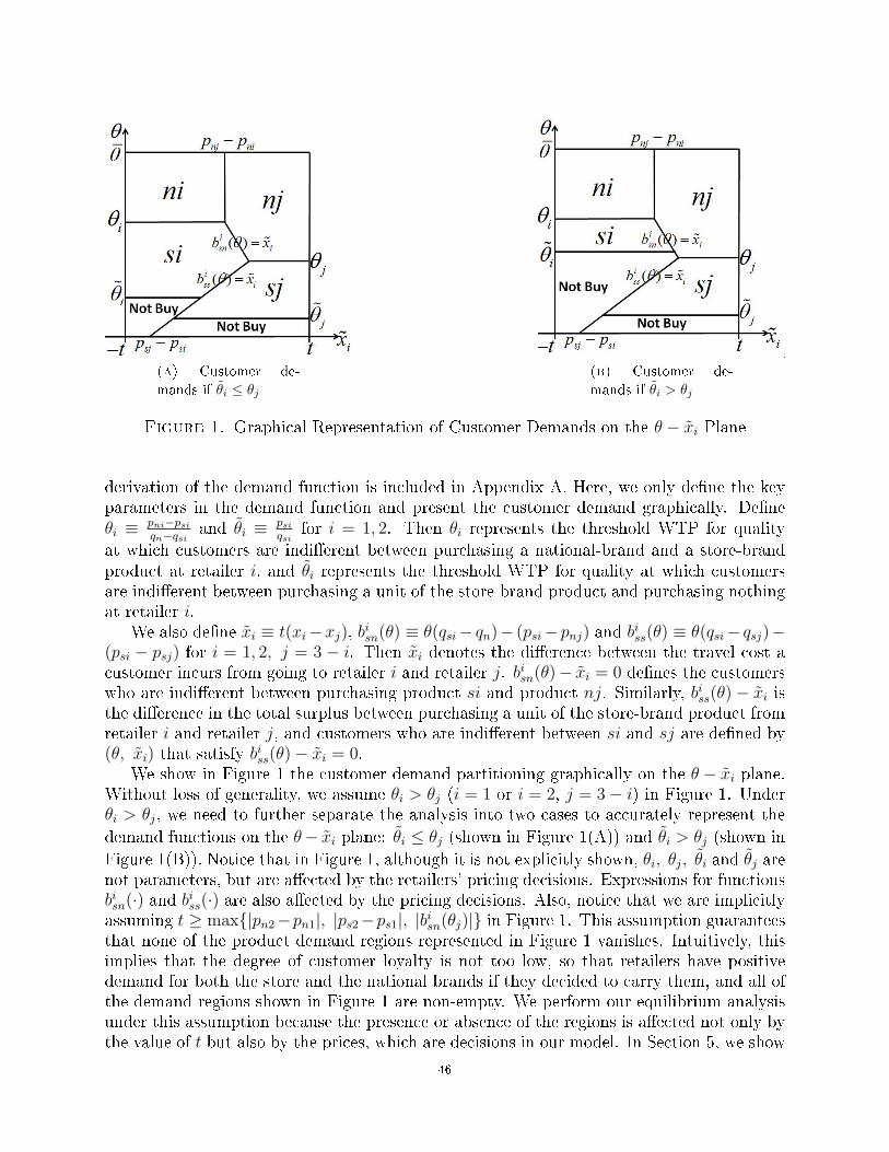
(a) Customer de-

mands if θi ≤ θj

(b) Customer de-

mands if θi > θj

Figure 1. Graphical Representation of Customer Demands on the θ − xi Plane

derivation of the demand function is included in Appendix A. Here, we only de�ne the keyparameters in the demand function and present the customer demand graphically. De�neθi ≡ pni−psi

qn−qsiand θi ≡ psi

qsifor i = 1, 2. Then θi represents the threshold WTP for quality

at which customers are indi�erent between purchasing a national-brand and a store-brandproduct at retailer i, and θi represents the threshold WTP for quality at which customersare indi�erent between purchasing a unit of the store-brand product and purchasing nothingat retailer i.

We also de�ne xi ≡ t(xi−xj), bisn(θ) ≡ θ(qsi− qn)− (psi−pnj) and biss(θ) ≡ θ(qsi− qsj)−

(psi − psj) for i = 1, 2, j = 3 − i. Then xi denotes the di�erence between the travel cost acustomer incurs from going to retailer i and retailer j. bisn(θ)− xi = 0 de�nes the customerswho are indi�erent between purchasing product si and product nj. Similarly, biss(θ)− xi isthe di�erence in the total surplus between purchasing a unit of the store-brand product fromretailer i and retailer j, and customers who are indi�erent between si and sj are de�ned by(θ, xi) that satisfy biss(θ)− xi = 0.

We show in Figure 1 the customer demand partitioning graphically on the θ − xi plane.Without loss of generality, we assume θi > θj (i = 1 or i = 2, j = 3− i) in Figure 1. Underθi > θj, we need to further separate the analysis into two cases to accurately represent the

demand functions on the θ− xi plane: θi ≤ θj (shown in Figure 1(A)) and θi > θj (shown in

Figure 1(B)). Notice that in Figure 1, although it is not explicitly shown, θi, θj, θi and θj arenot parameters, but are a�ected by the retailers' pricing decisions. Expressions for functionsbisn(·) and biss(·) are also a�ected by the pricing decisions. Also, notice that we are implicitlyassuming t ≥ max{|pn2−pn1|, |ps2−ps1|, |bisn(θj)|} in Figure 1. This assumption guaranteesthat none of the product demand regions represented in Figure 1 vanishes. Intuitively, thisimplies that the degree of customer loyalty is not too low, so that retailers have positivedemand for both the store and the national brands if they decided to carry them, and all ofthe demand regions shown in Figure 1 are non-empty. We perform our equilibrium analysisunder this assumption because the presence or absence of the regions is a�ected not only bythe value of t but also by the prices, which are decisions in our model. In Section 5, we show

46

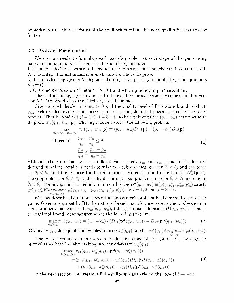
numerically that characteristics of the equilibrium retain the same qualitative features for�nite t.

3.3. Problem Formulation

We are now ready to formulate each party's problem at each stage of the game usingbackward induction. Recall that the stages in the game are:1. Retailer 1 decides whether to introduce a store brand and if so, chooses its quality level.2. The national brand manufacturer chooses its wholesale price.3. The retailers engage in a Nash game, choosing retail prices (and implicitly, which productsto o�er).4. Customers choose which retailer to visit and which product to purchase, if any.

The customers' aggregate response to the retailer's price decisions was presented in Sec-tion 3.2. We now discuss the third stage of the game.

Given any wholesale price wn > 0 and the quality level of R1's store brand product,qs1, each retailer sets its retail prices while observing the retail prices selected by the otherretailer. That is, retailer i (i = 1, 2, j = 3− i) seeks a pair of prices (pni, psi) that maximizeits pro�t πri(qs1, wn, p). That is, retailer i solves the following problem:

maxpni≥wn, psi≥csi

πri(qs1, wn, p) ≡ (pni − wn)Dni(p) + (psi − csi)Dsi(p)

subject topni − psiqn − qsi

≤ θ

psiqsi

≤ pni − psiqn − qsi

(1)

Although there are four prices, retailer i chooses only pni and psi. Due to the form ofdemand functions, retailer i needs to solve two subproblems, one for θi ≥ θj and the otherfor θi < θj, and then choose the better solution. Moreover, due to the form of DH

si (p, θ),

the subproblem for θi ≥ θj further divides into two subproblems, one for θi ≥ θj and one for

θi < θj. For any qs1 and wn, equilibrium retail prices p*(qs1, wn) ≡(p∗n1, p∗s1, p

∗n2, p

∗s2) satisfy

(p∗ni, p∗si)∈argmaxpni,psi≥0

πri(qs1, wn, (pni, psi, p∗nj, p

∗sj)) for i = 1, 2 and j = 3− i.

We now describe the national brand manufacturer's problem in the second stage of thegame. Given any qs1 set by R1, the national brand manufacturer selects the wholesale pricethat optimizes his own pro�t, πm(qs1, wn), taking into consideration p*(qs1, wn). That is,the national brand manufacturer solves the following problem:

maxwn≥cn

πm(qs1, wn) ≡ (wn − cn) · (Dn1(p*(qs1, wn)) +Dn2(p*(qs1, wn))) (2)

Given any qs1, the equilibrium wholesale price w∗n(qs1) satis�es w

∗n(qs1)∈argmax

wn≥0πm(qs1, wn).

Finally, we formulate R1's problem in the �rst stage of the game, i.e., choosing theoptimal store brand quality, taking into consideration w∗

n(qs1):

max0≤qs1≤qn

πr1(qs1, w∗n(qs1), p*(qs1, w∗

n(qs1)))

≡(pn1(qs1, w∗n(qs1))− w∗

n(qs1))Dn1(p*(qs1, w∗n(qs1)))

+ (ps1(qs1, w∗n(qs1))− cs1)Ds1(p*(qs1, w∗

n(qs1)))

(3)

In the next section, we present a full equilibrium analysis for the case of t → +∞.

47

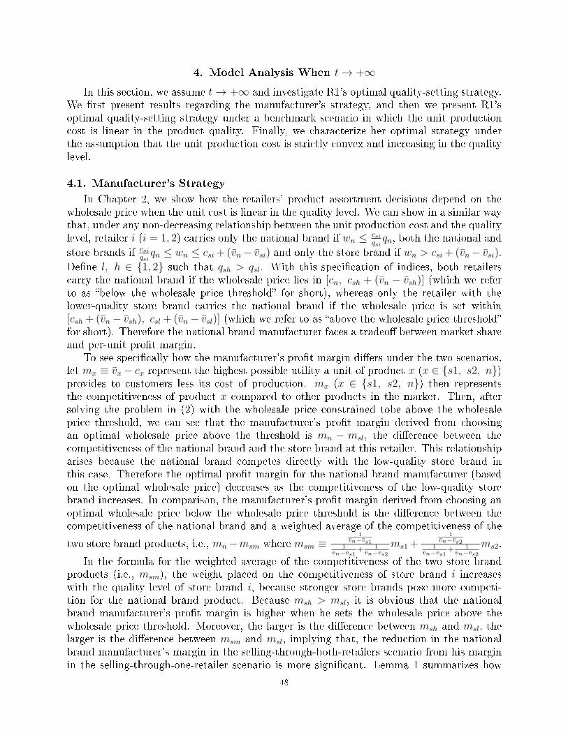
4. Model Analysis When t → +∞

In this section, we assume t → +∞ and investigate R1's optimal quality-setting strategy.We �rst present results regarding the manufacturer's strategy, and then we present R1'soptimal quality-setting strategy under a benchmark scenario in which the unit productioncost is linear in the product quality. Finally, we characterize her optimal strategy underthe assumption that the unit production cost is strictly convex and increasing in the qualitylevel.

4.1. Manufacturer's Strategy

In Chapter 2, we show how the retailers' product assortment decisions depend on thewholesale price when the unit cost is linear in the quality level. We can show in a similar waythat, under any non-decreasing relationship between the unit production cost and the qualitylevel, retailer i (i = 1, 2) carries only the national brand if wn ≤ csi

qsiqn, both the national and

store brands if csiqsiqn ≤ wn ≤ csi + (vn − vsi) and only the store brand if wn > csi + (vn − vsi).

De�ne l, h ∈ {1, 2} such that qsh > qsl. With this speci�cation of indices, both retailerscarry the national brand if the wholesale price lies in [cn, csh + (vn − vsh)] (which we referto as �below the wholesale price threshold� for short), whereas only the retailer with thelower-quality store brand carries the national brand if the wholesale price is set within[csh + (vn − vsh), csl + (vn − vsl)] (which we refer to as �above the wholesale price threshold�for short). Therefore the national brand manufacturer faces a tradeo� between market shareand per-unit pro�t margin.

To see speci�cally how the manufacturer's pro�t margin di�ers under the two scenarios,let mx ≡ vx − cx represent the highest possible utility a unit of product x (x ∈ {s1, s2, n})provides to customers less its cost of production. mx (x ∈ {s1, s2, n}) then representsthe competitiveness of product x compared to other products in the market. Then, aftersolving the problem in (2) with the wholesale price constrained tobe above the wholesaleprice threshold, we can see that the manufacturer's pro�t margin derived from choosingan optimal wholesale price above the threshold is mn − msl, the di�erence between thecompetitiveness of the national brand and the store brand at this retailer. This relationshiparises because the national brand competes directly with the low-quality store brand inthis case. Therefore the optimal pro�t margin for the national brand manufacturer (basedon the optimal wholesale price) decreases as the competitiveness of the low-quality storebrand increases. In comparison, the manufacturer's pro�t margin derived from choosing anoptimal wholesale price below the wholesale price threshold is the di�erence between thecompetitiveness of the national brand and a weighted average of the competitiveness of the

two store brand products, i.e., mn−msm where msm ≡1

vn−vs11

vn−vs1+ 1

vn−vs2

ms1+1

vn−vs21

vn−vs1+ 1

vn−vs2

ms2.

In the formula for the weighted average of the competitiveness of the two store brandproducts (i.e., msm), the weight placed on the competitiveness of store brand i increaseswith the quality level of store brand i, because stronger store brands pose more competi-tion for the national brand product. Because msh > msl, it is obvious that the nationalbrand manufacturer's pro�t margin is higher when he sets the wholesale price above thewholesale price threshold. Moreover, the larger is the di�erence between msh and msl, thelarger is the di�erence between msm and msl, implying that, the reduction in the nationalbrand manufacturer's margin in the selling-through-both-retailers scenario from his marginin the selling-through-one-retailer scenario is more signi�cant. Lemma 1 summarizes how

48

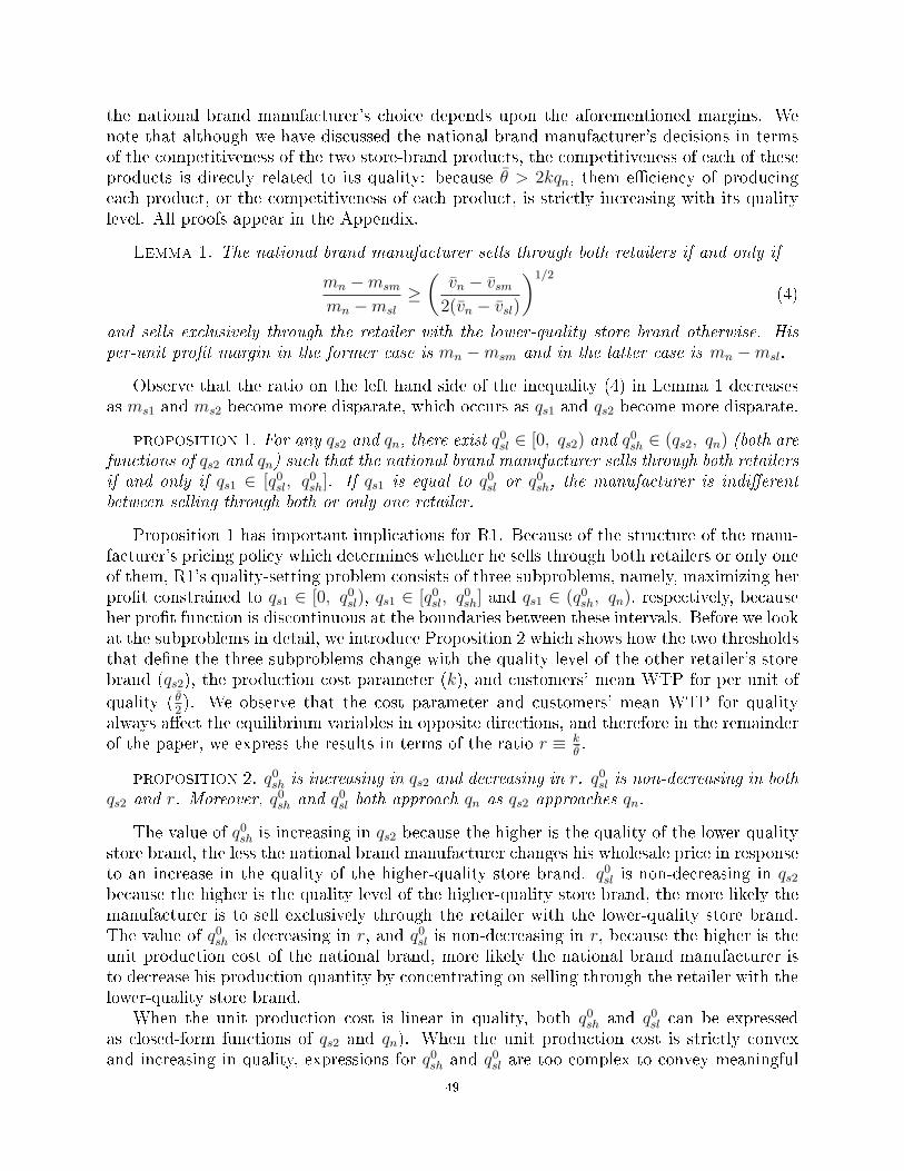
the national brand manufacturer's choice depends upon the aforementioned margins. Wenote that although we have discussed the national brand manufacturer's decisions in termsof the competitiveness of the two store-brand products, the competitiveness of each of theseproducts is directly related to its quality: because θ > 2kqn, them e�ciency of producingeach product, or the competitiveness of each product, is strictly increasing with its qualitylevel. All proofs appear in the Appendix.

Lemma 1. The national brand manufacturer sells through both retailers if and only if

mn −msm

mn −msl

≥(

vn − vsm2(vn − vsl)

)1/2

(4)

and sells exclusively through the retailer with the lower-quality store brand otherwise. Hisper-unit pro�t margin in the former case is mn −msm and in the latter case is mn −msl.

Observe that the ratio on the left hand side of the inequality (4) in Lemma 1 decreasesas ms1 and ms2 become more disparate, which occurs as qs1 and qs2 become more disparate.

proposition 1. For any qs2 and qn, there exist q0sl ∈ [0, qs2) and q0sh ∈ (qs2, qn) (both are

functions of qs2 and qn) such that the national brand manufacturer sells through both retailersif and only if qs1 ∈ [q0sl, q0sh]. If qs1 is equal to q0sl or q0sh, the manufacturer is indi�erentbetween selling through both or only one retailer.

Proposition 1 has important implications for R1. Because of the structure of the manu-facturer's pricing policy which determines whether he sells through both retailers or only oneof them, R1's quality-setting problem consists of three subproblems, namely, maximizing herpro�t constrained to qs1 ∈ [0, q0sl), qs1 ∈ [q0sl, q0sh] and qs1 ∈ (q0sh, qn), respectively, becauseher pro�t function is discontinuous at the boundaries between these intervals. Before we lookat the subproblems in detail, we introduce Proposition 2 which shows how the two thresholdsthat de�ne the three subproblems change with the quality level of the other retailer's storebrand (qs2), the production cost parameter (k), and customers' mean WTP for per unit of

quality ( θ2). We observe that the cost parameter and customers' mean WTP for quality

always a�ect the equilibrium variables in opposite directions, and therefore in the remainderof the paper, we express the results in terms of the ratio r ≡ k

θ.

proposition 2. q0sh is increasing in qs2 and decreasing in r. q0sl is non-decreasing in bothqs2 and r. Moreover, q0sh and q0sl both approach qn as qs2 approaches qn.

The value of q0sh is increasing in qs2 because the higher is the quality of the lower-qualitystore brand, the less the national brand manufacturer changes his wholesale price in responseto an increase in the quality of the higher-quality store brand. q0sl is non-decreasing in qs2because the higher is the quality level of the higher-quality store brand, the more likely themanufacturer is to sell exclusively through the retailer with the lower-quality store brand.The value of q0sh is decreasing in r, and q0sl is non-decreasing in r, because the higher is theunit production cost of the national brand, more likely the national brand manufacturer isto decrease his production quantity by concentrating on selling through the retailer with thelower-quality store brand.

When the unit production cost is linear in quality, both q0sh and q0sl can be expressedas closed-form functions of qs2 and qn). When the unit production cost is strictly convexand increasing in quality, expressions for q0sh and q0sl are too complex to convey meaningful

49

insights. However, we are able to show that they are bounded by some simple closed-formexpressions. We present all of the relevant expressions in Proposition 3.

proposition 3. When the unit production cost is linear in quality, q0sh = 23qn+

13qs2 and

q0sl = 3qs2 − 2qn. When the unit production cost is strictly increasing and convex in quality,3−

√5

2qn +

√5−12

qs2 < q0sh < 23qn +

13qs2 and 3qs2 − 2qn < q0sl <

√5+12

qs2 −√5−12

qn.

When the production cost is linear in quality, we can reexpress q0sh implicitly via theequality q0sh − qs2 = 2(qn − qs2) and similarly, q0sl via the equality qs2 − q0sl = 2(qn − qs2).We can then conclude that the manufacturer sells through both retailers if and only ifqsh − qsl < 2(qn − qsh), i.e., only if the quality disparity between the two store brands isbelow a threshold. Furthermore, it is clear that the threshold decreases with quality of thehigher-quality store brand. When the unit production cost is a quadratic function of thequality level, expressions for q0sh and q0sl are much more complex. But Proposition 3 says thatq0sh is bounded above by

23qn+

13qs2, where

23qn+

13qs2 is exactly q0sh derived under the scenario

in which the unit production cost is linear. Also, q0sh is bounded below by 3−√5

2qn +

√5−12

qs2

(≈ 0.38qn + 0.62qs2). One can easily con�rm that 3−√5

2qn +

√5−12

qs2 is exactly q0sh derived

under the scenario in which k = θ2qn

. (Recall that we assume k < θ2qn

so that the �e�ciency�

of producing a product increases with the product quality.) Similarly, q0sl is bounded belowby q0sl derived under the scenario in which unit production cost is linear, and bounded above

by q0sl derived under the scenario in which k = θ2qn

.

We next explain why the linear-unit-production-cost scenario and the k = θ2qn

scenarios

provide upper (lower) and lower (upper) bounds on q0sh and q0sl, respectively. When the unitproduction cost is linear in quality, producing one unit of the national brand is less costlythan when the unit production cost is strictly convex and increasing, therefore the regionin which the national brand manufacturer prefers to sell through both retailers (and hence

obtains a higher demand) expands. On the other hand, the solution for k = θ2qn

provides

a bound because we are interested in the region in which k < θ2qn

, and by using k = θ2qn

,we obtain a smaller region in which the national brand manufacturer prefers to sell throughboth retailers. In Figure 2, we present a numerical example showing q0sh and q0sl as functionsof qs2 when the unit production cost is strictly convex and increasing in quality. We useparameter values r = 0.4 and qn = 1 in this example. Figure 2 also shows the upper andlower bounds on q0sh and q0sl.

4.2. Retailer 1's Quality-Setting Strategy

We now examine the three subproblems that R1 needs to solve; she needs to choosethe best solution among them. When qs1 ∈ [0, q0sl) (i.e., in the low range), the nationalbrand manufacturer sets his price above the wholesale price threshold so as to sell throughR1 only and R1's pro�t is derived from her sales of both the store and national brands.When qs1 ∈ [q0sl, q

0sh] (i.e., in the medium range), R1's pro�t still comes from both products,

but the national brand manufacturer sets his price below the wholesale price threshold tocater to both retailers. When qs1 ∈ (q0sh, qn] (i.e., in the high range), the national brandmanufacturer sets the wholesale price above the threshold, so R1 chooses not to carry thenational brand and only carries its store brand.

Let πlr1(qs1) denote R1's pro�t function when qs1 is in the low range and its unconstrained

maximizer as qls1. Similarly, let πmr1(qs1) (π

hr1(qs1)) denote R1's pro�t function when qs1 is in

50

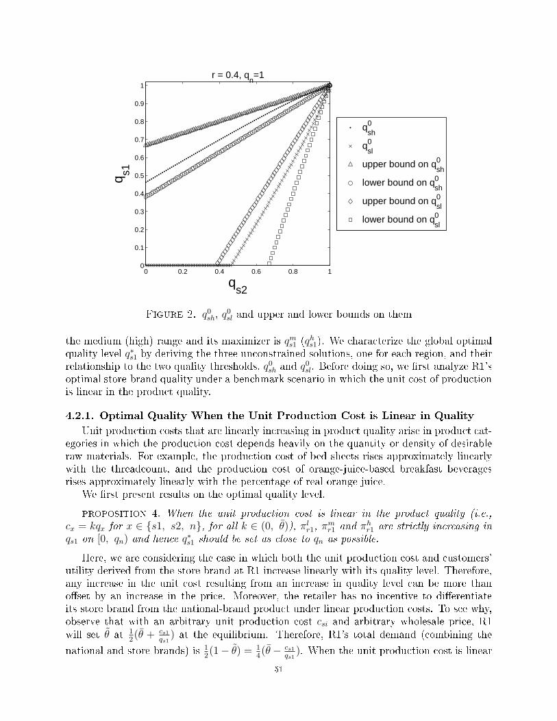
0 0.2 0.4 0.6 0.8 10

0.1

0.2

0.3

0.4

0.5

0.6

0.7

0.8

0.9

1

qs2

q s1

r = 0.4, qn=1

qsh0

qsl0

upper bound on qsh0

lower bound on qsh0

upper bound on qsl0

lower bound on qsl0

Figure 2. q0sh, q0sl and upper and lower bounds on them

the medium (high) range and its maximizer is qms1 (qhs1). We characterize the global optimal

quality level q∗s1 by deriving the three unconstrained solutions, one for each region, and theirrelationship to the two quality thresholds, q0sh and q0sl. Before doing so, we �rst analyze R1'soptimal store-brand quality under a benchmark scenario in which the unit cost of productionis linear in the product quality.

4.2.1. Optimal Quality When the Unit Production Cost is Linear in Quality

Unit production costs that are linearly increasing in product quality arise in product cat-egories in which the production cost depends heavily on the quantity or density of desirableraw materials. For example, the production cost of bed sheets rises approximately linearlywith the threadcount, and the production cost of orange-juice-based breakfast beveragesrises approximately linearly with the percentage of real orange juice.

We �rst present results on the optimal quality level.

proposition 4. When the unit production cost is linear in the product quality (i.e.,cx = kqx for x ∈ {s1, s2, n}, for all k ∈ (0, θ)), πl

r1, πmr1 and πh

r1 are strictly increasing inqs1 on [0, qn) and hence q∗s1 should be set as close to qn as possible.

Here, we are considering the case in which both the unit production cost and customers'utility derived from the store brand at R1 increase linearly with its quality level. Therefore,any increase in the unit cost resulting from an increase in quality level can be more thano�set by an increase in the price. Moreover, the retailer has no incentive to di�erentiateits store brand from the national-brand product under linear production costs. To see why,observe that with an arbitrary unit production cost csi and arbitrary wholesale price, R1will set θ at 1

2(θ + cs1

qs1) at the equilibrium. Therefore, R1's total demand (combining the

national and store brands) is 12(1− θ) = 1

4(θ− cs1

qs1). When the unit production cost is linear

51

in the product quality, cs1 = kqs1 and thus the total retail demand is 14(θ − k), which does

not change with the quality of her store brand. Thus, because quality di�erentiation hasno e�ect on total unit sales and R1 earns a higher pro�t margin from both the store-brandproduct (as explained above) and the national-brand product (because the national brandmanufacturer lowers his wholesale price in response to increased competition), R1 increasesthe quality of her store brand product to match that of the national brand product.

Although the retailer does not derive any value from di�erentiating her product fromthe national-brand product when the unit production cost is linear in the quality, she doesderive value from doing so when the unit production cost is strictly convex in the quality, aswe show in the next subsection.

4.2.2. Optimal Quality Level When the Unit Production Cost is StrictlyIncreasing and Convex in Quality

In this section, we discuss the optimal quality-setting strategy for R1 when the unit pro-duction cost is strictly convex and increasing in product quality. This cost relationship isapplicable in settings where increasingly higher quality requires increasingly rarer input ma-terials, skill, or technical sophistication to produce the product, such as cosmetics, computer�chips� or leather products. We assume costs have the form cs1 = kq2s1. Under this assump-tion, the total demand at R1 is 1

4(θ − cs1

qs1) = 1

4(θ − kqs1) which increases as qs1 decreases.

Therefore, under these conditions, by di�erentiating her store brand from the national brand,the retailer is able to achieve price discrimination between customers with high and low WTPper unit of quality and enjoy a larger demand base. However, the more di�erentiated thestore brand is from the national brand, the less competition the store brand poses for thenational brand manufacturer. Thus, R1 has an incentive to introduce a store brand that is aclose substitute for the national brand in order to gain the greatest price concession on thenational brand product. Thus, R1 faces a tradeo�; we elaborate further below.

When r is very low, the retailer incurs very low unit cost of producing a high-quality storebrand. She therefore always sets the quality level of her store brand at qn and sells the storebrand product exclusively. On the other hand, when r is greater than a threshold, the retailerprefers a quality level less than qn, which keeps the unit production cost down and allows theretailer to bene�t from some product di�erentiation. When making this decision, the retaileris aware that, depending on whether her store-brand quality level is much lower, much higher,or not much di�erent from the other store brand, the national brand manufacturer pricesdi�erently to induce either only her, only the other retailer, or both of them, to o�er thenational brand. The retailer's optimal choice of her store-brand quality therefore dependsheavily on the quality level of the store brand at the other retailer. Proposition 5 statesconditions under which the optimal quality level of the retailer in question falls into the low,medium and high intervals under the condition that r exceeds a threshold.

proposition 5. If r > 13qn

, there exist qs2(r) and qs2(r) such that q∗s1 takes a value in

[q0sh, qn] if qs2 ∈ [0, qs2(r)], a value in (q0sl, q0sh) if qs2 ∈ (qs2(r), qs2(r)) and a value in (0, q0sl]

if qs2 ∈ [qs2(r), qn).

This proposition states that for any r above the stated threshold, there is an interval ofhigh (medium, low) quality levels for R2's store brand product that maps to an interval oflow (medium, high) quality levels for R1's store brand product. It is also straightforward

52

to show that when R1's store brand quality takes a value in the medium range, the optimalvalue is strictly decreasing in qs2.

Intuitively, when the quality level of the other store brand is low (i.e., qs2 ∈ [0, qs2(r))),selling the national brand is not a good choice for R1. Recall that the national brandmanufacturer's optimal wholesale price increases as the weighted average of the competi-tiveness of the two store brands decreases. When qs2 is very low, the competitiveness ofthe store brand at R2 is very low, and hence the wholesale price charged by the nationalbrand manufacturer is very high because he faces little competition. R1 would prefer tocarry only her store brand in this scenario. If the quality level of the other store brand(s2) is moderate (qs2 ∈ (qs2(r), qs2(r))), on the other hand, not only is its competitivenesshigher, but the national brand manufacturer also puts more weight on it when calculat-ing the weighted average of the competitiveness of the two store brand products (because

msm =1

vn−vs11

vn−vs1+ 1

vn−vs2

ms1 +1

vn−vs21

vn−vs1+ 1

vn−vs2

ms2). As a result, R1 is able to obtain a fairly low

wholesale price from the national brand manufacturer. In this case she will carry both thenational brand and her store brand, while at the same time R2 also carries both products.Finally, if the quality level of the store brand at R2 is very high (qs2 ∈ (qs2(r), qn)), thenational brand manufacturer �nds it optimal to distribute through R1 exclusively and heaccomplishes this by setting a high wholesale price that only R1 �nds acceptable. Therefore,in this case, R1's optimal quality level is the one that maximizes πl

r1, and she is the onlyretailer to carry both products.

Now that we have established the conditions under which R1's optimal quality falls intoeach of the three intervals, we turn to the question of what value the optimal quality levelshould take in each region and how it changes with qs2 and r. Proposition 6 provides answersto these questions.

proposition 6. The optimal quality levels have the following properties: (i) Magnitudes

of qhs1 and qls1: qhs1 = 13r

and qh∗s1 = min{qhs1, qn}, qls1 = 19r[6 + qnr − (9 + 12qnr − 8q2nr

2)12 ]

and ql∗s1 = min{qls1, qn}. (ii) Relationship among qhs1, qls1 and qms1: qms1, q

ls1 < qhs1. Moreover,

if qs2 > qls1, then qms1 < qls1 < qhs1. (iii) How qhs1, qls1 and qms1 change with qs2: qhs1 and qls1 are

invariant in qs2, whereas qms1 is strictly decreasing in qs2; (iv) How qhs1, qls1 and qms1 change

with r: if qh∗s1 < qn, qh∗s1 and ql∗s1 are strictly decreasing in r. qms1 is decreasing in r if and only

if (qn − qms1)(qn − qms1 + 2(qn − qs2)) > q2n − q2s2.

Proposition 6 has several implications. First, from (iii), we see that qsh and qsl areinvariant in qs2. This can be explained as follows. First, when t → +∞ (so each retailerhas a large number of loyal customers), the level of customer demand at R1 is not a�ectedby the value of qs2. So a change in qs2 can only a�ect R1's pro�t through a change in thenational brand wholesale price. But, if R1 sets qs1 in the high range, R1 does not carrythe national brand at all. Therefore, R1's pro�t (when she sets qs1 in the high range) isinvariant in qs2. On the other hand, if R1 sets qs1 in the low range, the wholesale priceitself is invariant in qs2 (as the national brand manufacturer does not sell through R2). Asa result, R1's pro�t is also invariant in qs2 when qs1 is set in the low range. Second, from(ii), we see that qls1<q

hs1. The reason is that when R1 carries only the store brand, she sets

the quality at a level that caters to customers with relatively high WTP per unit of quality,but she is deterred from setting the quality level extremely high because of the convex andincreasing structure of the unit production cost. On the other hand, when R1 sets her qualitylevel in the low range, this corresponds to a setting in which she o�ers both products and

53

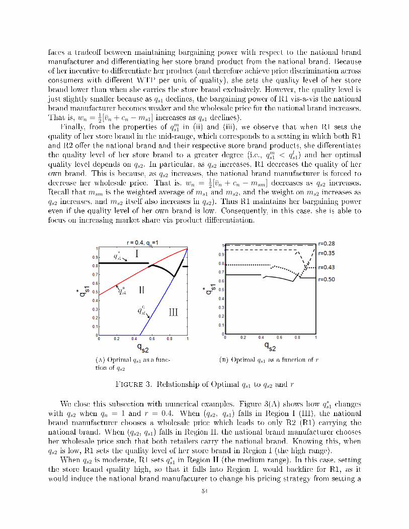
faces a tradeo� between maintaining bargaining power with respect to the national brandmanufacturer and di�erentiating her store-brand product from the national brand. Becauseof her incentive to di�erentiate her product (and therefore achieve price discrimination acrossconsumers with di�erent WTP per unit of quality), she sets the quality level of her storebrand lower than when she carries the store brand exclusively. However, the quality level isjust slightly smaller because as qs1 declines, the bargaining power of R1 vis-a-vis the nationalbrand manufacturer becomes weaker and the wholesale price for the national brand increases.That is, wn = 1

2[vn + cn −ms1] increases as qs1 declines).

Finally, from the properties of qms1 in (ii) and (iii), we observe that when R1 sets thequality of her store brand in the mid-range, which corresponds to a setting in which both R1and R2 o�er the national brand and their respective store brand products, she di�erentiatesthe quality level of her store brand to a greater degree (i.e., qms1 < qls1) and her optimalquality level depends on qs2. In particular, as qs2 increases, R1 decreases the quality of herown brand. This is because, as qs2 increases, the national brand manufacturer is forced todecrease her wholesale price. That is, wn = 1

2[vn + cn − msm] decreases as qs2 increases.

Recall that msm is the weighted average of ms1 and ms2, and the weight on ms2 increases asqs2 increases, and ms2 itself also increases in qs2). Thus R1 maintains her bargaining powereven if the quality level of her own brand is low. Consequently, in this case, she is able tofocus on increasing market share via product di�erentiation.

(a) Optimal qs1 as a func-tion of qs2

(b) Optimal qs1 as a function of r

Figure 3. Relationship of Optimal qs1 to qs2 and r

We close this subsection with numerical examples. Figure 3(A) shows how q∗s1 changeswith qs2 when qn = 1 and r = 0.4. When (qs2, qs1) falls in Region I (III), the nationalbrand manufacturer chooses a wholesale price which leads to only R2 (R1) carrying thenational brand. When (qs2, qs1) falls in Region II, the national brand manufacturer choosesher wholesale price such that both retailers carry the national brand. Knowing this, whenqs2 is low, R1 sets the quality level of her store brand in Region I (the high range).

When qs2 is moderate, R1 sets q∗s1 in Region II (the medium range). In this case, setting

the store brand quality high, so that it falls into Region I, would back�re for R1, as itwould induce the national brand manufacturer to change his pricing strategy from setting a

54

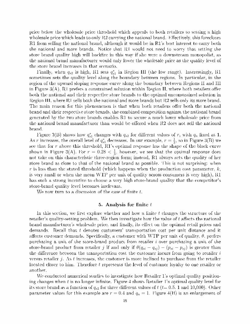
price below the wholesale price threshold which appeals to both retailers to setting a highwholesale price which leads to only R2 carrying the national brand. E�ectively, this foreclosesR1 from selling the national brand, although it would be in R1's best interest to carry boththe national and store brands. Notice that R1 would not need to worry that setting thestore brand quality high will back�re in this way if she were a downstream monopolist, asthe national brand manufacturer would only lower the wholesale price as the quality level ofthe store brand increases in that scenario.

Finally, when qs2 is high, R1 sets q∗s1 in Region III (the low range). Interestingly, R1sometimes sets the quality level along the boundary between regions. In particular, in theregion of the upward sloping response curve along the boundary between Regions II and IIIin Figure 3(A), R1 prefers a constrained solution within Region II, where both retailers o�erboth the national and their respective store brands to the optimal unconstrained solution inRegion III, where R1 sells both the national and store brands but R2 sells only its store brand.The main reason for this phenomenon is that when both retailers o�er both the nationalbrand and their respective store brands, the combined competition against the national brandgenerated by the two store brands enables R1 to secure a much lower wholesale price fromthe national brand manufacturer than would be o�ered when R2 does not sell the nationalbrand.

Figure 3(B) shows how q∗s1 changes with qs2 for di�erent values of r, with qn �xed at 1.As r increases, the overall level of q∗s1 decreases. In our example, r = 1

3, so in Figure 3(B) we

see that for r above this threshold, R1's optimal response has the shape of the black curveshown in Figure 3(A). For r = 0.28 < 1

3, however, we see that the optimal response does

not take on this characteristic three-region form; instead, R1 always sets the quality of herstore brand as close to that of the national brand as possible. This is not surprising: whenr is less than the stated threshold (which happens when the production cost parameter, k,is very small or when the mean WTP per unit of quality across consumers is very high), R1has such a strong incentive to choose a very high store-brand quality that the competitor'sstore-brand quality level becomes irrelevant.

We now turn to a discussion of the case of �nite t.

5. Analysis for �nite t

In this section, we �rst explore whether and how a �nite t changes the structure of theretailer's quality-setting problem. We then investigate how the value of t a�ects the nationalbrand manufacturer's wholesale price, and �nally, its e�ect on the optimal retail prices anddemands. Recall that t denotes customers' transportation cost per unit distance and ita�ects customer demands. Speci�cally, a customer with WTP per unit of quality, θ, preferspurchasing a unit of the store-brand product from retailer i over purchasing a unit of thestore-brand product from retailer j if and only if θ(qsi − qsj) − (psi − psj) is greater thanthe di�erence between the transportation cost the customer incurs from going to retailer iversus retailer j. As t increases, the customer is more inclined to purchase from the retailerlocated closer to him. Therefore t represents the level of customer loyalty to one retailer oranother.

We conducted numerical studies to investigate how Retailer 1's optimal quality position-ing changes when t is no longer in�nite. Figure 4 shows Retailer 1's optimal quality level forits store brand as a function of qs2 for three di�erent values of t (t= 0.5, 1 and 10,000). Otherparameter values for this example are r = 0.4 and qn = 1. Figure 4(B) is an enlargement of

55

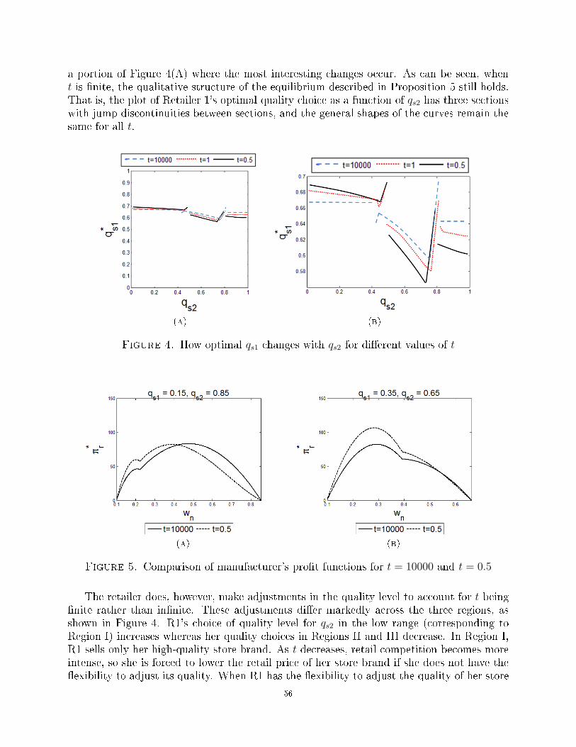
a portion of Figure 4(A) where the most interesting changes occur. As can be seen, whent is �nite, the qualitative structure of the equilibrium described in Proposition 5 still holds.That is, the plot of Retailer 1's optimal quality choice as a function of qs2 has three sectionswith jump discontinuities between sections, and the general shapes of the curves remain thesame for all t.

(a) (b)

Figure 4. How optimal qs1 changes with qs2 for di�erent values of t

(a) (b)

Figure 5. Comparison of manufacturer's pro�t functions for t = 10000 and t = 0.5

The retailer does, however, make adjustments in the quality level to account for t being�nite rather than in�nite. These adjustments di�er markedly across the three regions, asshown in Figure 4. R1's choice of quality level for qs2 in the low range (corresponding toRegion I) increases whereas her quality choices in Regions II and III decrease. In Region I,R1 sells only her high-quality store brand. As t decreases, retail competition becomes moreintense, so she is forced to lower the retail price of her store brand if she does not have the�exibility to adjust its quality. When R1 has the �exibility to adjust the quality of her store

56

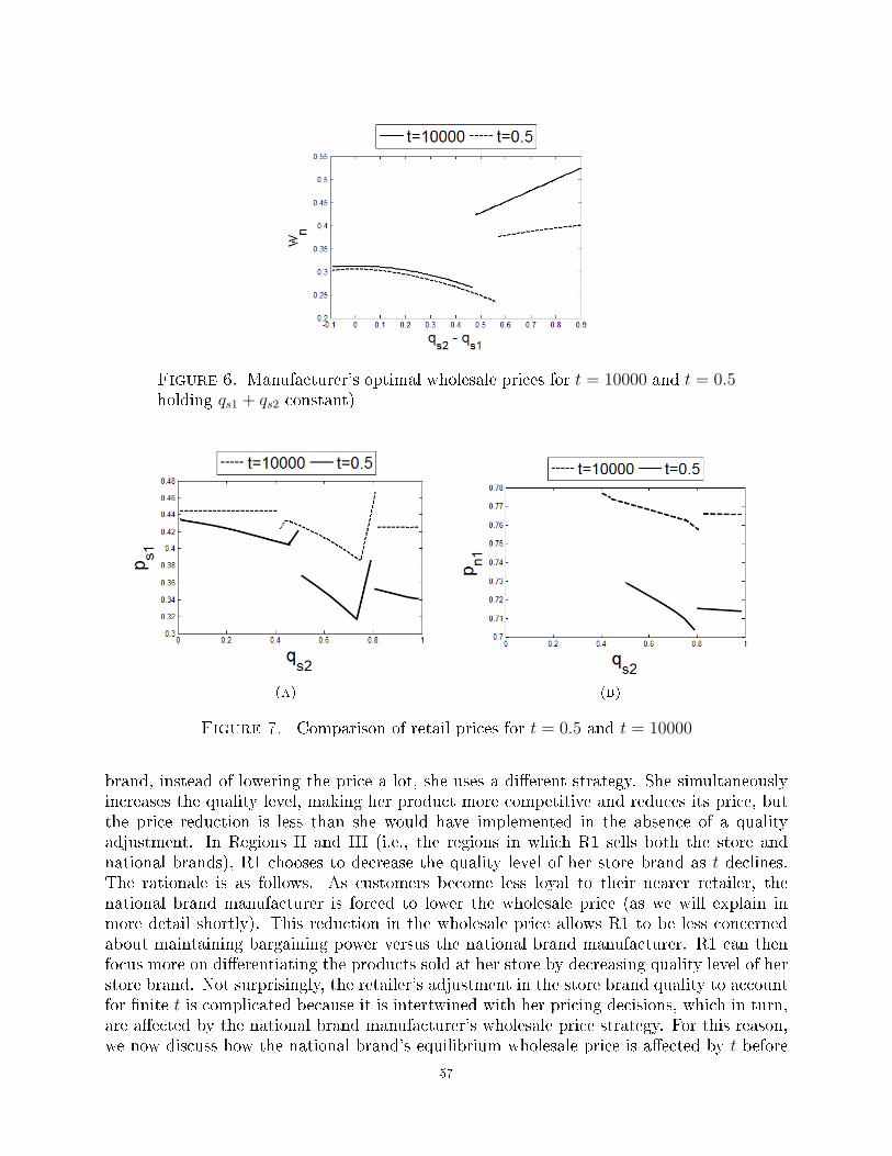
Figure 6. Manufacturer's optimal wholesale prices for t = 10000 and t = 0.5holding qs1 + qs2 constant)

(a) (b)

Figure 7. Comparison of retail prices for t = 0.5 and t = 10000

brand, instead of lowering the price a lot, she uses a di�erent strategy. She simultaneouslyincreases the quality level, making her product more competitive and reduces its price, butthe price reduction is less than she would have implemented in the absence of a qualityadjustment. In Regions II and III (i.e., the regions in which R1 sells both the store andnational brands), R1 chooses to decrease the quality level of her store brand as t declines.The rationale is as follows. As customers become less loyal to their nearer retailer, thenational brand manufacturer is forced to lower the wholesale price (as we will explain inmore detail shortly). This reduction in the wholesale price allows R1 to be less concernedabout maintaining bargaining power versus the national brand manufacturer. R1 can thenfocus more on di�erentiating the products sold at her store by decreasing quality level of herstore brand. Not surprisingly, the retailer's adjustment in the store brand quality to accountfor �nite t is complicated because it is intertwined with her pricing decisions, which in turn,are a�ected by the national brand manufacturer's wholesale price strategy. For this reason,we now discuss how the national brand's equilibrium wholesale price is a�ected by t before

57

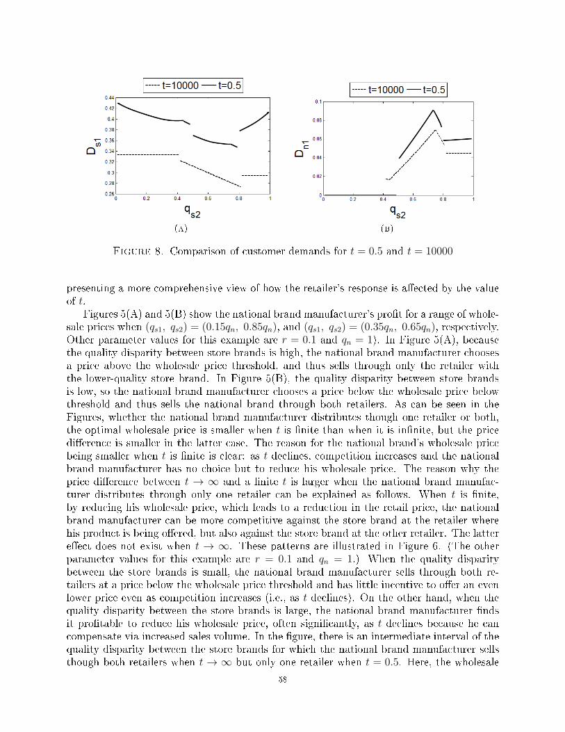
(a) (b)

Figure 8. Comparison of customer demands for t = 0.5 and t = 10000

presenting a more comprehensive view of how the retailer's response is a�ected by the valueof t.

Figures 5(A) and 5(B) show the national brand manufacturer's pro�t for a range of whole-sale prices when (qs1, qs2) = (0.15qn, 0.85qn), and (qs1, qs2) = (0.35qn, 0.65qn), respectively.Other parameter values for this example are r = 0.1 and qn = 1). In Figure 5(A), becausethe quality disparity between store brands is high, the national brand manufacturer choosesa price above the wholesale price threshold, and thus sells through only the retailer withthe lower-quality store brand. In Figure 5(B), the quality disparity between store brandsis low, so the national brand manufacturer chooses a price below the wholesale price belowthreshold and thus sells the national brand through both retailers. As can be seen in theFigures, whether the national brand manufacturer distributes though one retailer or both,the optimal wholesale price is smaller when t is �nite than when it is in�nite, but the pricedi�erence is smaller in the latter case. The reason for the national brand's wholesale pricebeing smaller when t is �nite is clear: as t declines, competition increases and the nationalbrand manufacturer has no choice but to reduce his wholesale price. The reason why theprice di�erence between t → ∞ and a �nite t is larger when the national brand manufac-turer distributes through only one retailer can be explained as follows. When t is �nite,by reducing his wholesale price, which leads to a reduction in the retail price, the nationalbrand manufacturer can be more competitive against the store brand at the retailer wherehis product is being o�ered, but also against the store brand at the other retailer. The lattere�ect does not exist when t → ∞. These patterns are illustrated in Figure 6. (The otherparameter values for this example are r = 0.1 and qn = 1.) When the quality disparitybetween the store brands is small, the national brand manufacturer sells through both re-tailers at a price below the wholesale price threshold and has little incentive to o�er an evenlower price even as competition increases (i.e., as t declines). On the other hand, when thequality disparity between the store brands is large, the national brand manufacturer �ndsit pro�table to reduce his wholesale price, often signi�cantly, as t declines because he cancompensate via increased sales volume. In the �gure, there is an intermediate interval of thequality disparity between the store brands for which the national brand manufacturer sellsthough both retailers when t → ∞ but only one retailer when t = 0.5. Here, the wholesale

58

price di�erential is signi�cant and is mostly due to a change in the national brand manu-facturer's retail distribution strategy and but also partly due to a change in the degree ofcompetition.

Now that we have a better understanding of how the national brand manufacturer'swholesale price is a�ected by t, we can examine how equilibrium retail prices and demanddemands are a�ected by t. With this as a backdrop, we next provide a more detailedexplanation of the reasons underlying the retailer's equilibrium quality choices, using Figures7 and 8 to illustrate our results. These two �gures show (1) R1's equilibrium retail prices(respectively, demands) at the optimal quality level for t → +∞ and (2) R1's optimal retailprices (demands) at the optimal quality level for t = 0.5. Other parameter values for thisexample are r = 0.5 and qn = 1.

Earlier in this section, we explained why R1 chooses a higher quality level in Region Iwhen t is �nite than when t is in�nite: she increases the quality to avoid a large price decreasein the face of increased competition. We now explain why the optimal quality level in RegionI is decreasing in qs2 for a �xed, �nite t. The logic is as follows. As the retailer increases herquality level in response to t being small, she su�ers from a reduction in customer demand(compared to that in the absence of a quality adjustment) As qs2 increases, R2's store brandbecomes more competitive, so each increment in qs1 (and the corresponding price increasefor product s1) causes a greater reduction in demand for R1. Therefore, when t is �nite, asqs2 increases in Region I, R1 decreases her optimal qs1. This, together with the phenomenonmentioned earlier, that is, R1's optimal qs1 in Region I when t is �nite is greater than thatwhen t is +∞ (for all value of qs2), explains the change in qs1 in Region I as t declines from+∞ to a �nite value.

In Regions II and III, R1's optimal reaction to a smaller t is dramatically di�erent thanin Region I: her store brand quality level is smaller for �nite t. In both of these regions,the retailer carries both the national and store brands. In Region I, R1 does not carry thenational brand. Therefore the change in the wholesale price does not a�ect her quality-positioning decision as directly as it did in Regions II and III. Due to the change in thenational brand manufacturer's wholesale price in Regions II and III, the retailer decreasesher quality. To complement the lower quality level, she sets a lower store brand retail priceand a higher national brand price than in the case of t → +∞, as illustrated in Figure7(B)). In essence, when there is sti� competition (small t), the retailer adopts a strategyof di�erentiating the two products so as to increase market share, and is aided by thenational brand manufacturer's choice of a relatively low wholesale price in response to thecompetition. We note that R1's demands in Region II di�er from those in Region III (seeFigure 8) because R2 o�ers a lower price on her store brand in Region II (where both retailero�er both the national brand and their respective store brand products) than in Region III(where R2 carries only the store brand).

We close this section by exploring whether R1 can safely choose her store brand qualitylevel assuming t → +∞ if all of the subsequent pricing decisions are made optimally con-ditional on the suboptimal quality level and the true t. Using the same numerical examplementioned above (with θ = 1, qn = 1), we calculate, for all values of qs2, the retailer's per-centage pro�t reduction when she ignores the �niteness of t when deciding the store-brandquality (but other decisions are made based on the true value of t) from the optimal pro�tlevel when all decisions are made optimally for t = 0.5. For our example, we �nd that

59

when the retailer's suboptimal quality level does not trigger the national brand manufac-turer to choose a di�erent distribution strategy, the retailer's pro�t reduction is less than0.3%. When the value of qs2 is such that, if the retailer makes quality positioning decisionsub-optimally, the national brand manufacturer uses a di�erent distribution strategy thanhe would when under the optimal quality decision, the percentage reduction in R1's pro�tis less than 0.96%. For this example, in both cases, the retailer's pro�t loss is small. Thissuggests that the optimal quality in the t → +∞ case can serve as a good starting point forthe retailer to search for optimal store brand quality when the true t is �nite.

6. Retailer 1's Preference about qs2

In the previous section, we derived R1's optimal quality decision when t → +∞ andshowed through numerical studies that the structure of her optimal quality decision does notchange signi�cantly when t is �nite. From a numerical example, we also observed that R1'spercentage pro�t reduction if she sets the quality level ignoring the �niteness of t but makesthe subsequent pricing decisions optimally, is relatively small.

One interesting question to ask is: what is R1's preference regarding the value of qs2?We present R1's equilibrium pro�t as a function of qs2 in Figures 9(A) and 9(B) for the casesof t → ∞ and t = 0.5, respectively. Other parameters for this example are r = 0.5 andqn = 1. In both �gures, the retailer's pro�t is calculated assuming that she sets quality andprices optimally. In Figure 9(C), we display the pro�t functions from Figures 9(A) and 9(B)together using the same scale to facilitate comparison.

When t → +∞, the retailer prefers that qs2 take the largest value within Region II. Thereason is that in Region II, any increase in qs2 forces the national brand manufacturer tolower the national brand wholesale price. As qs2 increases within Region II, R1 enjoys thebene�t of a lowered national brand wholesale price without having to increase her own storebrand quality level, which in turn, allows her to enjoy a larger market share. This bene�tdoes not exist in the other two regions. If the value of qs2 is high enough that it falls inRegion III, the national brand manufacturer sets a high wholesale price and sells throughR1 only. If the value of qs2 is low enough that it falls in Region I, R2's store brand productdoes not pose enough competition for the national brand product to induce the nationalbrand manufacturer to o�er a wholesale price that is su�ciently attractive to R1. Thus,although R2 o�ers a store brand product, R1 does not get the bene�t of a �free ride� fromprice concessions made by the national brand manufacturer in response to R2's store brandproduct. R1 thus chooses to sell her store brand only.

In contrast, when t = 0.5, R1 prefers qs2 to take the lowest possible value. There aretwo reasons. First, if qs2 is very low, the store brand at R2 is much less competitive thanthe store brand at R1. Therefore R1 is able to gain more market share. This e�ect does notexist when t is in�nite. Second, if qs2 is very low, the national brand manufacturer will seta very high wholesale price. This leads R2 to set a high price on the national brand, which,in turn, reduces the competitiveness of the national brand at R2. Many customers locatednear R2 will then choose to buy products at R1. This e�ect also does not exist when t isin�nite.

Comparing R1's pro�t when t is in�nity and when t is 0.5 in Figure 9(C), we �ndsome interesting phenomena. If qs2 is either very low or very high, R1's optimal pro�t whencustomers are not very loyal (represented by the t = 0.5 scenario) is greater than her optimalpro�t when customers are strictly loyal to the retailer located nearer them (represented by

60

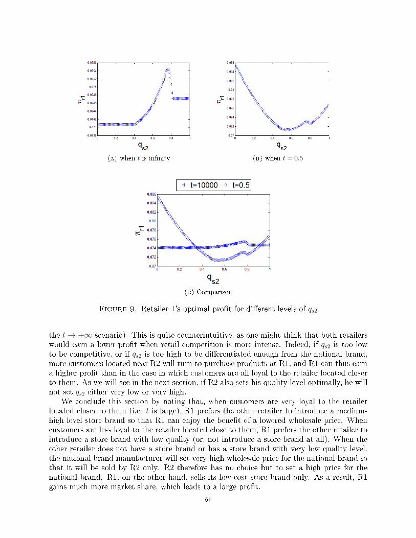
(a) when t is in�nity (b) when t = 0.5

(c) Comparison

Figure 9. Retailer 1's optimal pro�t for di�erent levels of qs2

the t → +∞ scenario). This is quite counterintuitive, as one might think that both retailerswould earn a lower pro�t when retail competition is more intense. Indeed, if qs2 is too lowto be competitive, or if qs2 is too high to be di�erentiated enough from the national brand,more customers located near R2 will turn to purchase products at R1, and R1 can thus earna higher pro�t than in the case in which customers are all loyal to the retailer located closerto them. As we will see in the next section, if R2 also sets his quality level optimally, he willnot set qs2 either very low or very high.

We conclude this section by noting that, when customers are very loyal to the retailerlocated closer to them (i.e. t is large), R1 prefers the other retailer to introduce a medium-high level store brand so that R1 can enjoy the bene�t of a lowered wholesale price. Whencustomers are less loyal to the retailer located close to them, R1 prefers the other retailer tointroduce a store brand with low quality (or, not introduce a store brand at all). When theother retailer does not have a store brand or has a store brand with very low quality level,the national brand manufacturer will set very high wholesale price for the national brand sothat it will be sold by R2 only. R2 therefore has no choice but to set a high price for thenational brand. R1, on the other hand, sells its low-cost store brand only. As a result, R1gains much more market share, which leads to a large pro�t.

61

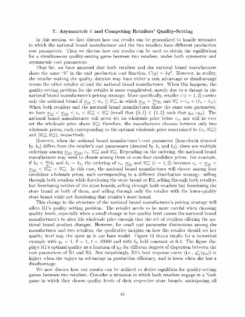
7. Asymmetric k and Competing Retailers' Quality-Setting

In this section, we �rst discuss how our results can be generalized to handle scenariosin which the national brand manufacturer and the two retailers have di�erent productioncost parameters. Then we discuss how our results can be used to obtain the equilibriumfor a simultaneous quality-setting game between two retailers, under both symmetric andasymmetric cost parameters.

Thus far, we have assumed that both retailers and the national brand manufacturershare the same �k� in the unit production cost function, C(q) = kq2. However, in reality,the retailer making the quality decision may have either a cost advantage or disadvantageversus the other retailer or/and the national brand manufacturer. When this happens, thequality-setting problem for the retailer is more complicated, mostly due to a change in thenational brand manufacturer's pricing strategy. More speci�cally, retailer i (i = 1, 2) carriesonly the national brand if wni ≤ wn ≤ wni, in which wni =

csiqsiqn and wn = csi + (vn − vsi).

When both retailers and the national brand manufacturer share the same cost parameter,we have wnl < wnh < cn < wnh < wnl (recall that {h, l} ∈ {1, 2} such that qsh>qsl). Thenational brand manufacturer will never set its wholesale price below cn, nor will he everset the wholesale price above wnl; therefore, the manufacturer chooses between only twowholesale prices, each corresponding to the optimal wholesale price constrained to (cn, wnh)and [wnh, wnl), respectively.

However, when the national brand manufacturer's cost parameter (henceforth denotedby k0) di�ers from the retailer's cost parameters (denoted by k1 and k2), there are multipleorderings among wnl, wnh, cn, wnh and wnl. Depending on the ordering, the national brandmanufacturer may need to choose among three or even four candidate prices. For example,if k0 < qsl

qnkl and k1 = k2, the ordering of cn, wni and wni (i = 1, 2) becomes cn < wnl <

wnh < wnh < wnl. In this case, the national brand manufacturer will choose among fourcandidate wholesale prices, each corresponding to a di�erent distribution strategy: sellingthrough both retailers while foreclosing the store brand at R2, selling through both retailersbut foreclosing neither of the store brands, selling through both retailers but foreclosing thestore brand at both of them, and selling through only the retailer with the lower-qualitystore brand while not foreclosing that retailer's store brand.

This change in the structure of the national brand manufacturer's pricing strategy willa�ect R1's quality setting problem. The retailer needs to be more careful when choosingquality levels, especially when a small change in her quality level causes the national brandmanufacturer's to alter his wholesale price enough that the set of retailers o�ering the na-tional brand product changes. However, for small cost parameter distinctions among themanufacturer and two retailers, the qualitative insights on how the retailer should set herquality level stay the same as in our base model. Figure 10 shows results for a numericalexample with qn = 1, θ = 1, t = 10000 and with k0 held constant at 0.4. The �gure dis-plays R1's optimal quality as a function of qs2 for di�erent degrees of dispersion between thecost parameters of R1 and R2. Not surprisingly, R1's best response curve (i.e., q∗s1(qs2)) ishigher when she enjoys an advantage in production e�ciency, and is lower when she has adisadvantage.

We now discuss how our results can be utilized to derive equilibria for quality-settinggames between two retailers. Consider a situation in which both retailers engage in a Nashgame in which they choose quality levels of their respective store brands, anticipating all

62

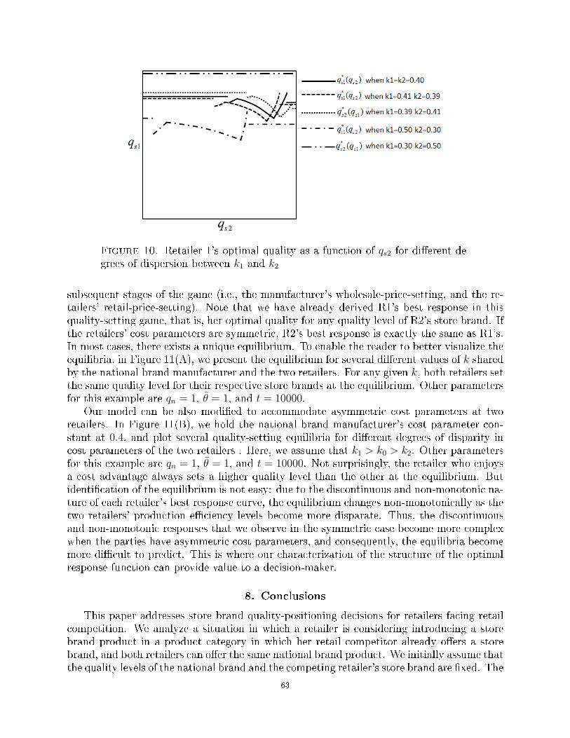
Figure 10. Retailer 1's optimal quality as a function of qs2 for di�erent de-grees of dispersion between k1 and k2

subsequent stages of the game (i.e., the manufacturer's wholesale-price-setting, and the re-tailers' retail-price-setting). Note that we have already derived R1's best response in thisquality-setting game, that is, her optimal quality for any quality level of R2's store brand. Ifthe retailers' cost parameters are symmetric, R2's best response is exactly the same as R1's.In most cases, there exists a unique equilibrium. To enable the reader to better visualize theequilibria, in Figure 11(A), we present the equilibrium for several di�erent values of k sharedby the national brand manufacturer and the two retailers. For any given k, both retailers setthe same quality level for their respective store brands at the equilibrium. Other parametersfor this example are qn = 1, θ = 1, and t = 10000.

Our model can be also modi�ed to accommodate asymmetric cost parameters at tworetailers. In Figure 11(B), we hold the national brand manufacturer's cost parameter con-stant at 0.4, and plot several quality-setting equilibria for di�erent degrees of disparity incost parameters of the two retailers . Here, we assume that k1 > k0 > k2. Other parametersfor this example are qn = 1, θ = 1, and t = 10000. Not surprisingly, the retailer who enjoysa cost advantage always sets a higher quality level than the other at the equilibrium. Butidenti�cation of the equilibrium is not easy: due to the discontinuous and non-monotonic na-ture of each retailer's best response curve, the equilibrium changes non-monotonically as thetwo retailers' production e�ciency levels become more disparate. Thus, the discontinuousand non-monotonic responses that we observe in the symmetric case become more complexwhen the parties have asymmetric cost parameters, and consequently, the equilibria becomemore di�cult to predict. This is where our characterization of the structure of the optimalresponse function can provide value to a decision-maker.

8. Conclusions

This paper addresses store brand quality-positioning decisions for retailers facing retailcompetition. We analyze a situation in which a retailer is considering introducing a storebrand product in a product category in which her retail competitor already o�ers a storebrand, and both retailers can o�er the same national brand product. We initially assume thatthe quality levels of the national brand and the competing retailer's store brand are �xed. The

63

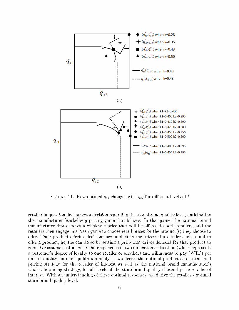
(a)

(b)

Figure 11. How optimal qs1 changes with qs2 for di�erent levels of t

retailer in question �rst makes a decision regarding the store-brand quality level, anticipatingthe manufacturer-Stackelberg pricing game that follows. In that game, the national brandmanufacturer �rst chooses a wholesale price that will be o�ered to both retailers, and theretailers then engage in a Nash game to choose retail prices for the product(s) they choose too�er. Their product o�ering decisions are implicit in the prices: if a retailer chooses not too�er a product, he/she can do so by setting a price that drives demand for that product tozero. We assume customers are heterogeneous in two dimensions�location (which representsa customer's degree of loyalty to one retailer or another) and willingness to pay (WTP) perunit of quality. in our equilibrium analysis, we derive the optimal product assortment andpricing strategy for the retailer of interest as well as the national brand manufacturer'swholesale pricing strategy, for all levels of the store brand quality chosen by the retailer ofinterest. With an understanding of these optimal responses, we derive the retailer's optimalstore-brand quality level.

64

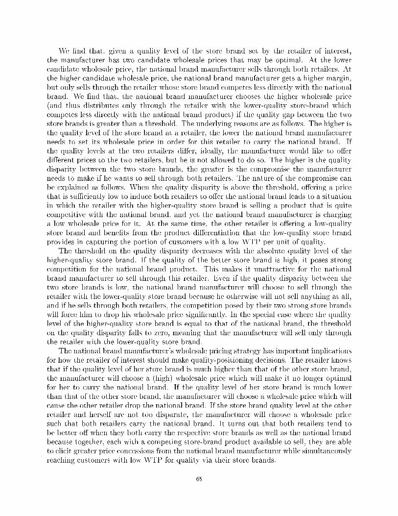
We �nd that, given a quality level of the store brand set by the retailer of interest,the manufacturer has two candidate wholesale prices that may be optimal. At the lowercandidate wholesale price, the national brand manufacturer sells through both retailers. Atthe higher candidate wholesale price, the national brand manufacturer gets a higher margin,but only sells through the retailer whose store brand competes less directly with the nationalbrand. We �nd that, the national brand manufacturer chooses the higher wholesale price(and thus distributes only through the retailer with the lower-quality store-brand whichcompetes less directly with the national brand product) if the quality gap between the twostore brands is greater than a threshold. The underlying reasons are as follows. The higher isthe quality level of the store brand at a retailer, the lower the national brand manufacturerneeds to set its wholesale price in order for this retailer to carry the national brand. Ifthe quality levels at the two retailers di�er, ideally, the manufacturer would like to o�erdi�erent prices to the two retailers, but he is not allowed to do so. The higher is the qualitydisparity between the two store brands, the greater is the compromise the manufacturerneeds to make if he wants to sell through both retailers. The nature of the compromise canbe explained as follows. When the quality disparity is above the threshold, o�ering a pricethat is su�ciently low to induce both retailers to o�er the national brand leads to a situationin which the retailer with the higher-quality store brand is selling a product that is quitecompetitive with the national brand, and yet the national brand manufacturer is charginga low wholesale price for it. At the same time, the other retailer is o�ering a low-qualitystore brand and bene�ts from the product di�erentiation that the low-quality store brandprovides in capturing the portion of customers with a low WTP per unit of quality.

The threshold on the quality disparity decreases with the absolute quality level of thehigher-quality store brand. If the quality of the better store brand is high, it poses strongcompetition for the national brand product. This makes it unattractive for the nationalbrand manufacturer to sell through this retailer. Even if the quality disparity between thetwo store brands is low, the national brand manufacturer will choose to sell through theretailer with the lower-quality store brand because he otherwise will not sell anything at all,and if he sells through both retailers, the competition posed by their two strong store brandswill force him to drop his wholesale price signi�cantly. In the special case where the qualitylevel of the higher-quality store brand is equal to that of the national brand, the thresholdon the quality disparity falls to zero, meaning that the manufacturer will sell only throughthe retailer with the lower-quality store brand.

The national brand manufacturer's wholesale pricing strategy has important implicationsfor how the retailer of interest should make quality-positioning decisions. The retailer knowsthat if the quality level of her store brand is much higher than that of the other store brand,the manufacturer will choose a (high) wholesale price which will make it no longer optimalfor her to carry the national brand. If the quality level of her store brand is much lowerthan that of the other store brand, the manufacturer will choose a wholesale price which willcause the other retailer drop the national brand. If the store brand quality level at the otherretailer and herself are not too disparate, the manufacturer will choose a wholesale pricesuch that both retailers carry the national brand. It turns out that both retailers tend tobe better o� when they both carry the respective store brands as well as the national brandbecause together, each with a competing store-brand product available to sell, they are ableto elicit greater price concessions from the national brand manufacturer while simultaneouslyreaching customers with low WTP for quality via their store brands.

65

The �ner details of the retailer's quality decision for her store-brand depend on how theunit production cost changes with the quality level. If the unit production cost of storebrand is linearly increasing in the product quality, the retailer always sets the quality levelof her store brand the same as that of the national brand. The underlying reason is thatwith a linear cost relationship, the retailer does not derive any value from di�erentiating herproduct from the national-brand product. Stated another way, the total number of unitsthat she sells does not change with the quality level of the store brand. The retailer thereforeincreases the quality level of the store brand and thus earns a higher pro�t margin on eachunit of the product sold.

On the other hand, if the unit production cost of is strictly convex and increasing inthe product quality, the retailer's quality decision becomes more complex, and it dependsheavily on the quality level of the store brand at the other retailer. Indeed, as the qualitylevel of the competing store brand increases, the optimal quality level set by the retailerof interest is non-monotonic and discontinuous. A small increase in the quality level of thecompeting store brand could lead to a �jump� in her optimal quality level. Speci�cally, ifthe quality level at the other retailer is low (high), the retailer will set the quality level ofher store brand in a high (low) range. If the quality level at the other retailer is moderate,the retailer will set the quality level of her store brand in the moderate range. When theretailer's quality level is within the either the high or the low range, her optimal qualitylevel is invariant with the quality level of the other store brand; whereas when her optimaloptimal quality level falls into the moderate range, the quality level is strictly decreasingwith the quality level of the store brand at the other retailer. Intuitively, as the quality levelof the other store brand increases, the national brand manufacturer is forced to reduce hiswholesale price. The retailer of interest thus has less incentive to increase quality, as herincentive to increase quality arises from her quest to obtain a lower wholesale price from thenational brand manufacturer.

Our results contribute to the literature by showing how the presence of retail competitionleads to optimal store brand quality-positioning strategies that can be quite di�erent from thecommon wisdom but also much more complex than what has been reported in past research..The past literature on store brand strategies has suggested that a monopolist retailer shouldset the quality level of her store brand as high as possible, as it can increase her bargainingpower versus the national brand manufacturer. We �nd this is not the case if the retaileris facing competition. Under retail competition, setting a high quality level for the storebrand can back�re. In particular, increasing the quality level of the store brand does notnecessarily increase a retailer's bargaining power. If the retailer sets too high a quality level,the national brand manufacturer could charge a high wholesale price, e�ectively foreclosingthe retailer of interest from selling the national brand (because it is uneconomical for theretailer to o�er the national brand product), although it would have been in the retailer'sbest interest to sell a moderate- or low-quality store brand product alongside the nationalbrand product.

We also study how the intensity of competition a�ects the equilibrium. As retail compe-tition becomes more heated, the retailer adjusts the quality level of her store brand in orderto alleviate price competition between the product(s) sold at her store and the product(s)sold at the other retailer. More speci�cally, if it is optimal for the retailer to carry only thestore brand at her store (which occurs if the other store brand is low in quality), she wouldincrease the quality level of her store brand to become more di�erentiated from the store

66

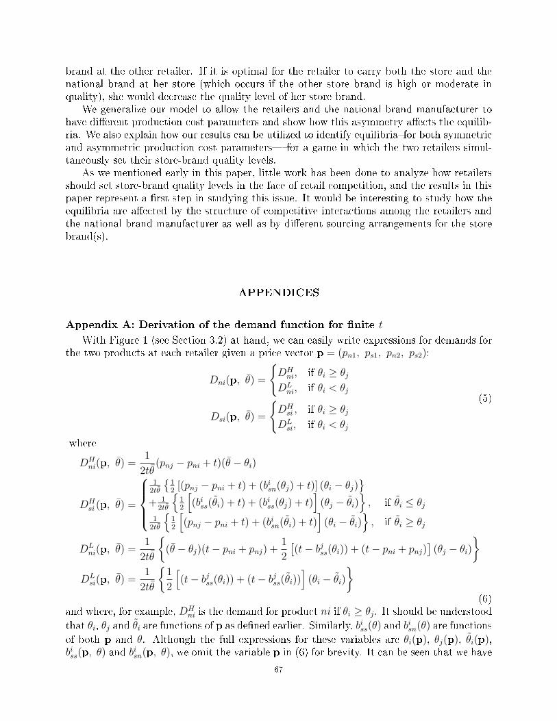
brand at the other retailer. If it is optimal for the retailer to carry both the store and thenational brand at her store (which occurs if the other store brand is high or moderate inquality), she would decrease the quality level of her store brand.

We generalize our model to allow the retailers and the national brand manufacturer tohave di�erent production cost parameters and show how this asymmetry a�ects the equilib-ria. We also explain how our results can be utilized to identify equilibria�for both symmetricand asymmetric production cost parameters� for a game in which the two retailers simul-taneously set their store-brand quality levels.

As we mentioned early in this paper, little work has been done to analyze how retailersshould set store-brand quality levels in the face of retail competition, and the results in thispaper represent a �rst step in studying this issue. It would be interesting to study how theequilibria are a�ected by the structure of competitive interactions among the retailers andthe national brand manufacturer as well as by di�erent sourcing arrangements for the storebrand(s).

APPENDICES

Appendix A: Derivation of the demand function for �nite t

With Figure 1 (see Section 3.2) at hand, we can easily write expressions for demands forthe two products at each retailer given a price vector p = (pn1, ps1, pn2, ps2):

Dni(p, θ) =

{DH

ni, if θi ≥ θj

DLni, if θi < θj

Dsi(p, θ) =

{DH

si , if θi ≥ θjDL

si, if θi < θj

(5)

where

DHni(p, θ) =

1

2tθ(pnj − pni + t)(θ − θi)

DHsi (p, θ) =

12tθ

{12[(pnj − pni + t) + (bisn(θj) + t)] (θi − θj)

}+ 1

2tθ

{12

[(biss(θi) + t) + (biss(θj) + t)

](θj − θi)

}, if θi ≤ θj

12tθ

{12

[(pnj − pni + t) + (bisn(θi) + t)

](θi − θi)

}, if θi ≥ θj

DLni(p, θ) =

1

2tθ

{(θ − θj)(t− pni + pnj) +

1

2

[(t− bjss(θi)) + (t− pni + pnj)

](θj − θi)

}DL

si(p, θ) =1

2tθ

{1

2

[(t− bjss(θi)) + (t− bjss(θi))

](θi − θi)

}(6)

and where, for example, DHni is the demand for product ni if θi ≥ θj. It should be understood

that θi, θj and θi are functions of p as de�ned earlier. Similarly, biss(θ) and bisn(θ) are functions

of both p and θ. Although the full expressions for these variables are θi(p), θj(p), θi(p),biss(p, θ) and bisn(p, θ), we omit the variable p in (6) for brevity. It can be seen that we have

67

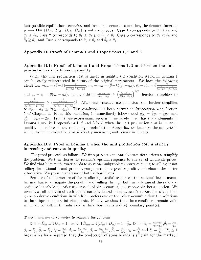
four possible equilibrium scenarios, and from one scenario to another, the demand functionp 7−→ D≡ (Dn1, Ds1, Dn2, Ds2) is not continuous. Case 1 corresponds to θ1 ≥ θ2 and

θ1 ≥ θ2, Case 2 corresponds to θ1 ≥ θ2 and θ1 < θ2, Case 3 corresponds to θ1 < θ2 andθ2 ≥ θ1, and Case 4 corresponds to θ1 < θ2 and θ2 < θ1.

Appendix B: Proofs of Lemma 1 and Propositions 1, 2 and 3

Appendix B.1: Proofs of Lemma 1 and Propositions 1, 2 and 3 when the unitproduction cost is linear in quality

When the unit production cost is linear in quality, the condition stated in Lemma 1can be easily reinterpreted in terms of the original parameters. We have the followingidentities: msm = (θ−k) 2

1qn−qs1

+ 1qn−qs2

, mn−msl = (θ−k)(qn−qsl), vn− ¯vsm = θ 21

qn−qs1+ 1

qn−qs2

and vn − vl = θ(qn − qsl). The condition mn−msm

mn−msl≥

(vn−vsm2(vn−vsl)

)1/2

therefore simpli�es to2

qn−qsl1

qn−qs1+ 1

qn−qs2

≥ (1

qn−qsl1

qn−qs1+ 1

qn−qs2

)12 . After mathematical manipulation, this further simpli�es

to qsh − qsl ≤ 2(qn − qsh). This condition has been derived in Proposition 4 in Section5 of Chapter 2. From this condition, it immediately follows that q0sh = 2

3qn + 1

3qs2 and

q0sl = 3qs2 − 2qn. From these expressions, we can immediately infer that the statements inLemma 1 and in Propositions 1, 2 and 3 hold when the unit production cost is linear inquality. Therefore, in the remaining proofs in this Appendix, we focus on the scenario inwhich the unit production cost is strictly increasing and convex in quality.

Appendix B.2: Proof of Lemma 1 when the unit production cost is strictlyincreasing and convex in quality

The proof proceeds as follows. We �rst present some variable transformations to simplifythe problem. We then derive the retailer's optimal response to any set of wholesale prices.We �nd that he manufacturer needs to solve two subproblems, corresponding to selling or notselling the national brand product, compare their respective pro�ts, and choose the betteralternative. We present analyses of both subproblems.

Because of the structure of the retailer's potential responses, the national brand manu-facturer has to anticipate the possibility of selling through both or only one of the retailers,optimize his wholesale price under each of the scenarios, and choose the better option. Wepresent a full analysis of each of the national brand manufacturer's subproblems and thengo on to derive conditions in which he prefers one or the other assuming that the solutionsto the subproblems are interior points. Finally, we show that these conditions remain validwhen one or both of the solutions to the subproblems is (are) boundary point(s).

Transformation of variables to simplify the problem

De�ne Dni ≡ 2Dni = 1−ϕi and Dnsi ≡ 2(Dni+Dsi) = 1− ϕi. De�ne θi =pni−psiqn−qsi

,θi =psiqsi,

ϕi =θiθ, ϕi =

θiθ, bi =

qsiqn, di =

qn−qsiqn

, βi =wn−csiθqn

, βi =csiθqn

, γi =βi

diand γi =

βi

bi. (γi ≤ 1

because we have assumed that the production of store brands is e�cient for the market.)

68

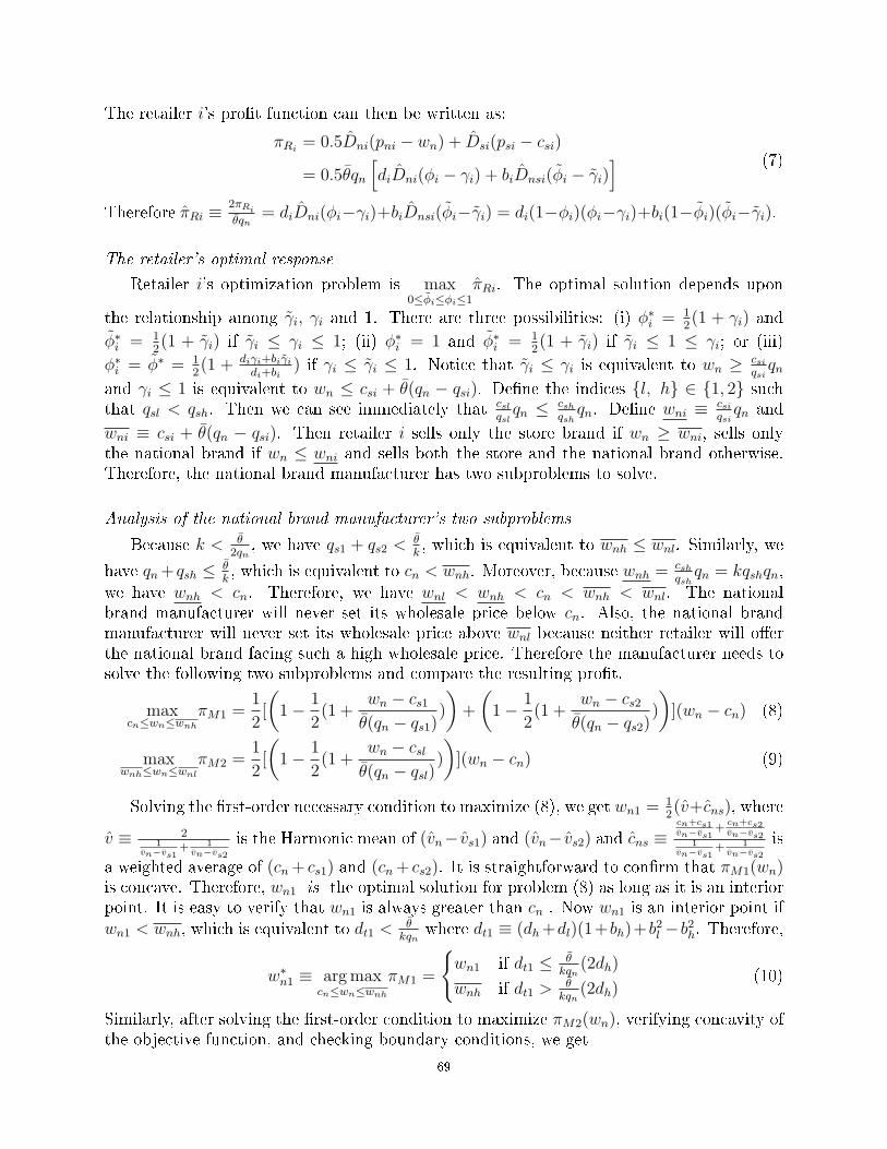
The retailer i's pro�t function can then be written as:

πRi= 0.5Dni(pni − wn) + Dsi(psi − csi)

= 0.5θqn

[diDni(ϕi − γi) + biDnsi(ϕi − γi)

] (7)

Therefore πRi ≡2πRi

θqn= diDni(ϕi−γi)+biDnsi(ϕi−γi) = di(1−ϕi)(ϕi−γi)+bi(1−ϕi)(ϕi−γi).

The retailer's optimal response

Retailer i's optimization problem is max0≤ϕi≤ϕi≤1

πRi. The optimal solution depends upon

the relationship among γi, γi and 1. There are three possibilities: (i) ϕ∗i = 1

2(1 + γi) and

ϕ∗i = 1

2(1 + γi) if γi ≤ γi ≤ 1; (ii) ϕ∗

i = 1 and ϕ∗i = 1

2(1 + γi) if γi ≤ 1 ≤ γi; or (iii)

ϕ∗i = ϕ∗ = 1

2(1 + diγi+biγi

di+bi) if γi ≤ γi ≤ 1. Notice that γi ≤ γi is equivalent to wn ≥ csi

qsiqn

and γi ≤ 1 is equivalent to wn ≤ csi + θ(qn − qsi). De�ne the indices {l, h} ∈ {1, 2} suchthat qsl < qsh. Then we can see immediately that csl

qslqn ≤ csh

qshqn. De�ne wni ≡ csi

qsiqn and

wni ≡ csi + θ(qn − qsi). Then retailer i sells only the store brand if wn ≥ wni, sells onlythe national brand if wn ≤ wni and sells both the store and the national brand otherwise.Therefore, the national brand manufacturer has two subproblems to solve.

Analysis of the national brand manufacturer's two subproblems

Because k < θ2qn

, we have qs1 + qs2 <θk, which is equivalent to wnh ≤ wnl. Similarly, we

have qn+ qsh ≤ θk, which is equivalent to cn < wnh. Moreover, because wnh = csh

qshqn = kqshqn,

we have wnh < cn. Therefore, we have wnl < wnh < cn < wnh < wnl. The nationalbrand manufacturer will never set its wholesale price below cn. Also, the national brandmanufacturer will never set its wholesale price above wnl because neither retailer will o�erthe national brand facing such a high wholesale price. Therefore the manufacturer needs tosolve the following two subproblems and compare the resulting pro�t.

maxcn≤wn≤wnh

πM1 =1

2[

(1− 1

2(1 +

wn − cs1θ(qn − qs1)

)

)+

(1− 1

2(1 +

wn − cs2θ(qn − qs2)

)

)](wn − cn) (8)

maxwnh≤wn≤wnl

πM2 =1

2[

(1− 1

2(1 +

wn − cslθ(qn − qsl)

)

)](wn − cn) (9)

Solving the �rst-order necessary condition to maximize (8), we get wn1 =12(v+cns), where

v ≡ 21

vn−vs1+ 1

vn−vs2

is the Harmonic mean of (vn− vs1) and (vn− vs2) and cns ≡cn+cs1vn−vs1

+cn+cs2vn−vs2

1vn−vs1

+ 1vn−vs2

is

a weighted average of (cn+ cs1) and (cn+ cs2). It is straightforward to con�rm that πM1(wn)is concave. Therefore, wn1 is the optimal solution for problem (8) as long as it is an interiorpoint. It is easy to verify that wn1 is always greater than cn . Now wn1 is an interior point ifwn1 < wnh, which is equivalent to dt1 <

θkqn

where dt1 ≡ (dh+dl)(1+bh)+b2l −b2h. Therefore,

w∗n1 ≡ argmax

cn≤wn≤wnh

πM1 =

{wn1 if dt1 ≤ θ

kqn(2dh)

wnh if dt1 >θ

kqn(2dh)

(10)

Similarly, after solving the �rst-order condition to maximize πM2(wn), verifying concavity ofthe objective function, and checking boundary conditions, we get

69

w∗n2 ≡ argmax

cn≤wnh≤wnl

πM2 =

{wn2 if dt2 ≥ θ

kqn(2dh − dl)

wnh if dt2 <θ

kqn(2dh − dl)

(11)

where wn2 =12[(cn + csl) + (vn − vsl)] and dt2 ≡ dh(1 + bh) + (b2l − b2h).

It is straightforward to show that if the condition for w∗n1 = wnh is satis�ed, then we

must have w∗n2 = wn2. Also, if the condition for w∗

n2 = wnh is satis�ed, then we must havew∗

n1 = wn1. Therefore, we have

(w∗n1, w∗

n2) =

(wn1, wn2) if dt1 ≤ θ

kqn(2dh) and dt2 ≥ θ

kqn(2dh − dl)

(wnh, wn2) if dt1 >θ

kqn(2dh)

(wn1, wnh) if dt2 <θ

kqn(2dh − dl)

(12)

Conditions in which the manufacturer prefers one of the subproblem solutions when bothare interior

Both w∗n1 and w∗

n2 take the corresponding interior solution when dt1 ≤ θkqn

(2dh) and

dt2 ≥ θkqn

(2dh − dl),. The manufacturer compares the pro�ts from the two solutions and

chooses the better one. The manufacturer's pro�t is π∗M1 = 1

8v(v + csm − cn)

2 at wn1 and

π∗M2 =

116(vn−vsl)

(vn− vsl+csl−cn)2 at wn2. De�ne vsm ≡ vn− v =

vs1vn−vs1

+vs2

vn−vs21

vn−vs1+ 1

vn−vs2

, the weighted

average of vs1 and vs2, and de�ne csm ascs1

vn−vs1+

cs2vn−vs2

1vn−vs1

+ 1vn−vs2

, that is, the weighted average of cs1 and

cs2. Then we can express π∗M1 as

18(vn−vsm)

((vn− cn)− (vm− csm))2. Also de�ne mx ≡ vx− cx

for x ∈ {n, s1, s2, sm}. That is, mx is the utility that product x provides to a customerless its production cost. Then{

π∗M1 = 1

8(vn−vsm)(mn −msm)

2

π∗M2 = 1

16(vn−vsl)(mn −msl)

2(13)

In this way, we have constructed an �aggregate� product, sm, whose competitiveness,msm, is

the weighted average of the competitiveness of s1 and s2. From (13), we conclude that whenthe solution to both of the manufacturer's subproblems, (8) and (9), are interior points,

the manufacturer sets the wholesale price at wn1 when mn−msm

mn−msl≥

(vn−vsm2(vn−vsl)

)1/2

and the

wholesale price at wn2 otherwise.

Proof that the results remain the same when the solution to either subproblem is on aboundary

As stated earlier, the manufacturer's pro�t functions with the wholesale price constrainedto either below or above the threshold, πM1(wn) and πM2(wn) (as de�ned in (8) and (9)),are both concave. Hence his pro�t function is piecewise concave. Also, his pro�t functionis continuous on [cn, wnl]. Therefore, when the solution of one subproblem is an interiorpoint and the solution of the other subproblem is a boundary solution, the interior solutionis optimal. We need to show that, when this is the case, the condition the �optimal solution

w∗n1 is chosen over w∗

n2 ifmn−msm

mn−msl≥

(vn−vsm2(vn−vsl)

)1/2

� still holds. That is, what remains to be

70

proved are two relationships: (1) w∗n1 = wnh ⇒ ( mn−msl

mn−msm)2 ≥ 2(vn−vsl)

vn−vsmand (2) w∗

n2 = wnh ⇒( mn−msl

mn−msm)2 ≤ 2(vn−vsl)

vn−vsm.

To facilitate the proof, we de�ne fi ≡ 1vn−vsi

for i = 1, 2; y ≡ qsh−qslqn−qsl

; α ≡1

vn−vsh1

vn−vsh+ 1

vn−vsl

and x ≡ msh−msl

mn−msl. Clearly, y ∈ (0, 1), α ∈ (1

2, 1) and x ∈ (0, 1). Moreover, we can

express relationships among fi, x, y, α and the mx's (for x ∈ {s1, s2, n}) as α ≡ 12−y

, x ≡y · (1−r·2qsl)−r(qn−qsl)y

1−r(qn+qsl), mn−msh

msh−msl≡ 1

x−1, (vn−vsm)

2(vn−vsl)= fl

f1+f2= 1−α, and (mn−msm

mn−msl)2 = (1−αx)2.

To show (1), note that w∗n1 = wnh if and only if f1+f2

fl< msh−msl

mn−msh. Moreover, 2(vn−vsl)

vn−vsm=

f1+f2fl

. Therefore we only need to show that ( mn−msl

mn−msm)2 ≥ msh−msl

mn−msh, which is equivalent to

mn−msh

msh−msl≥ (mn−msm

mn−msl)2. Rewriting the last inequality in terms of x and α, the condition

becomes 1x− 1 ≥ (1−αx)2. Now, because x ∈ (0, 1), a su�cient condition for the inequality

to hold is 1− x = x( 1x− 1) ≥ (1− αx)2, which is equivalent to x ≤ 2α−1

α2 = y(2− y). Now,substituting for x and dividing both sides of the inequality by y, the condition becomes(1−r·2qsl)−r(qn−qsl)y

1−r(qn+qsl)≤ 2− y, i.e., 2 ≥ (1−2rqsl)+y(1−2rqn)

1−r(qn+qsl). This is always true because the right-

hand-side in increasing in y and equals 2 when y = 1.To show (2), we �rst note that w∗

n2 = wnh if and only if mn − 2msh + msl > 0, orequivalently mn −msl > 2msh − 2msl, which can then be rewritten as msh−msl

mn−msl< 1

2. That is,

x < 12. Also, using the de�nition of α and x, we can express (vn−vsm)

2(vn−vsl)as 1 − α and express

(mn−msm

mn−msl)2 as (1 − αx)2. Hence, ( mn−msl

mn−msm)2 ≤ 2(vn−vsl)

vn−vsmis equivalent to (1 − αx)2 ≥ 1 − α.

Therefore, to establish our claim, we only need to show that x < 12⇒ (1 − αx)2 ≥ 1 − α.

This is obviously true because α ∈ (12, 1) and x ∈ (0, 1).

Appendix B.3: Proof of Proposition 1 when the unit production cost is strictlyincreasing and convex in quality

We need to show that for any �xed qsl and qn, there exists a unique q0sh ≡ q0sh(qsl, qn) ∈(qsl, qn) at which ( mn−msl

mn−msm)2 = 2(vn−vsl)

vn−vsmis satis�ed, and that for any �xed qsh and qn,

there exists a unique q0sl ≡ q0sl < qsh at which ( mn−msl

mn−msm)2 = 2(vn−vsl)

vn−vsmis satis�ed. We de�ne

y ≡ qsh−qslqn−qsl

as in the proof of Lemma 1. Also de�ne y ≡ 1− y = qn−qshqn−qsl

and z1 ≡ 1−2rqsl1−r(qn+qsl)

(∈(1, 2)). After tedious mathematical manipulation, one can show that (i) at any qsh ∈ (qsl, qn)

that constitutes a solution to ( mn−msl

mn−msm)2 = 2(vn−vsl)

vn−vsm, the corresponding y ≡ qsh−qsl

qn−qsl∈ (0, 1)

is the solution toz1y − (z1 − 1)y2 =

√2− y(

√2− y −

√1− y); (14)

and (ii) at any qsl < qsh that constitutes a solution to ( mn−msl

mn−msm)2 = 2(vn−vsl)

vn−vsm, the correspond-

ing y ≡ qn−qshqn−qsl

∈ (0, 1) is the solution to

1− y · 1− r(qn + qsh)

1− r(2qn − qn−qshy

)=

√1 + y(

√1 + y −

√y) (15)

Then we only need to show that both (14) and (15) have a unique solution (y and y,respectively) within (0, 1). The left hand side of (14) is increasing and concave in y andpasses though (0, 0) and (1, 1), whereas the right hand side is increasing and convex in y

71

and passes through (0, 2 −√2) and (1, 1). Therefore, for all z1 ∈ (1, 2), there exists a

unique y0 within (0, 1) that satis�es the above equation.Both the left and right hand sides of (15) are decreasing in y and both cross (0,1).

However, at y = 1, the left hand side is smaller than the right hand side. This implies thatthere exists a solution to (15) with y ∈ (0, 1) that value is the solution. It is straightforwardto verify that the left-hand-side is concave and the right-hand-side is convex. Therefore thesolution within (0,1) is unique. However, if the solution to (15) falls below 1 − qsh

qn, the qsl

corresponding to the solution y is negative. In this case, q0sl should be equal to zero. Astrictly positive q0sl exists if and only if the solution to (15) is greater than 1− qsh

qn.

Appendix B.4: Proof of Proposition 2 when the unit production cost is strictlyincreasing and convex in quality

In this proof, we show that q0sh(qsl, qn) is increasing in qsl and decreasing in r. The prooffor q0sl(qsl, qn) being an increasing function of both qsh and r is similar.

We �rst show that q0sh(qsl, qn) increases in qsl. The proof consists of three steps. First,we show z1 is decreasing in qsl. Second, we show that the solution to (14), y0, is decreasing inz1. These two statements together imply that y0 is increasing in qsl. Then, in the third step,we show that y0 being increasing in qsl implies that qsh is increasing in qsl. To establish thestatement in the �rst step, notice that d z1

d qsl= − r(1−2rqn)

[1−r(qn+qsl)]2< 0. Therefore z1 is decreasing

in qsl. To prove the claim in the second step, we can rewrite (14) as z1 = 1+ 1y(2−

√1 + 1

1−y).

As y increases, both 1 + 11−y

and 1ydecreases, therefore z1 decreases. For the statement in

the third step, we can rewrite the expression de�ning y, i.e., y = qsh−qslqn−qsl

, as qn − qsh =

(qn − qsl)(1− y). As we just showed, as qsl increases, y increases. Therefore, as qsl increases,(qn − qsl)(1 − y) increases (i.e., the right-hand side of the last equation increases), whichimplies that the left-hand side of the last equation (i.e., qn− qsh) increases. This proves thatqsh decreases as qsl increases, which is the statement in the third step.

Next, we show that q0sh(qsl, qn) is decreasing in r. As r increases, z1 increases, andtherefore the solution to (14), y0, decreases (because y0 is decreasing in z1, as noted earlier).This implies that q0sh is decreasing in r.

Appendix B.5: Proof of Proposition 3 when the unit production cost is strictlyincreasing and convex in quality

In this proof, we derive upper and lower bounds on q0sh and q0sl when the unit productioncost is strictly increasing and convex in quality. Expressions for q0sh and q0sl have been derivedin Chapter 2 when the unit production cost is linear and convex in quality, it is obvious thatqs1 = q0sl(qs2) and qs1 = q0sl(qs2) are symmetric on the qs1 − qs2 plane with respect to theline qs1 = qs2. In other words, qs1 = q0sl(qs2) and qs1 = q0sl(qs2) are inverse functions of eachother. Also, notice that the lower (upper) bound provided for qs1 = q0sl(qs2) is symmetricwith the upper (lower) bound provided for qs1 = q0sl(qs2) with respect to the line qs1 = qs2on the qs1 − qs2 plane. In other words, the lower (upper) bound provided for qs1 = q0sl(qs2)and the upper (lower) bound provided for qs1 = q0sl(qs2) are inverse functions of each other.Therefore, we only need to show that the upper and lower bound provided for q0sh are valid.

From the proof of Proposition 2, we know that q0sh can be found by solving z1 = 1 +1y[2 − (1 + 1

1−y)12 ]. From the de�nition of z1 in the proof of Proposition 1, we know z1 ∈

72

(1, 2). (We have z1 > 1 because qsl < qn and z1 < 2 because k < θ2qn

.) This implies that1y[2− (1+ 1

1−y)12 ] ∈ (0, 1). Via tedious mathematical manipulation, it can be shown that this

condition is equivalent to y ∈ (3−√5

2, 23). Using the fact that y = qsh−qsl

qn−qsl(as de�ned earlier),

y < 23and y > 3−

√5

2can be transformed to the respective upper and lower bounds on q0sh

provided in the statement of Proposition 3.

Appendix C: Proof of Proposition 4

The retailer solves three subproblems and chooses the one that provides the highestpro�t. In this proof, we �rst present the three subproblems R1 needs to solve, assumingan arbitrary increasing relationship between the unit production cost and the quality level.Then, we show that when the unit production cost is linearly increasing in product quality,R1's pro�t function is strictly increasing in the quality of her store brand.

Under unit production costs that are general increasing functions of the product quality,R1 solves the following three subproblems.

maxqs1

πhr1 ≡

qs14qn

(1− kqs1θ

)2 s.t. qs1 > q0sh(qs2, qn)

maxqs1

πlr1 ≡

d14(1−

12(vn − vs1 + cn + cs1)− cs1

vn − vs1)2 +

b14(1− cs1

vs1)2

s.t. qs1 < max(q0sl(qs2, qn), 0

)maxqs1

πmr1 ≡

d14(1−

12(vn − vsm + cn + csm)− cs1

vn − vs1)2 +

b14(1− cs1

vs1)2

s.t. max(q0sl(qs2, qn), 0

)≤ qs1 ≤ q0sh(qs2)

where πhr1 is R1's pro�t if qs1 is set at a (high) level such that the national brand manufacturer

responds with a wholesale price that is unattractive to R1, so R1 does not o�er the nationalbrand; πl

r1 is R1's pro�t if qs1 is in an intermediate range and the national brand manufacturerprices at wn1, leading both retailers to o�er the national brand product; πm

r1 is R1's pro�t ifqs1 is set low enough that the national brand manufacturer prices at wn2, which is attractiveto R1 but not to R2, so only R1 sells the national brand product.

Now, suppose that cx = kqx for x = s1, s2, n. Then, with some algebra, we obtain

πlr1 = qs1

4qn(1 − kqs1

θ)2 = qs1

4qn(1 − r)2, πh

r1 = d14(1 −

12(vn−vs1+cn+cs1)−cs1

vn−vs1)2 + b1

4(1 − cs1

vs1)2 =

qn−qs14qn

(1−r2)2 + qs1

4(1 − r)2 = (1−r)2(qn+3qs1)

16qnand πm

r1 = d14(1 −

12(vn−vsm+cn+csm)−cs1

vn−vs1)2 + b1

4(1 −

cs1vs1

)2 = qn−qs14qn

(1−r2

− 12

qs1−qs2qn−qs1+qn−qs2

(1 − r))2 + qs14(1 − r)2. Obviously the optimal solutions

to both πlr1 and πh

r1 is qn because these pro�t functions are strictly increasing in qsi. Now

πmr1 can be written as πm

r1 =(1−r)2

16qn[4qn − 2(qn − qs1) − 2(qn−qs2)

1+qn−qs2qn−qs1

]2, which is also increasing in

qs1. So we have established that when the unit production cost is linearly increasing in theproduct quality, R1 should set qs1 to the maximum possible quality level.

73

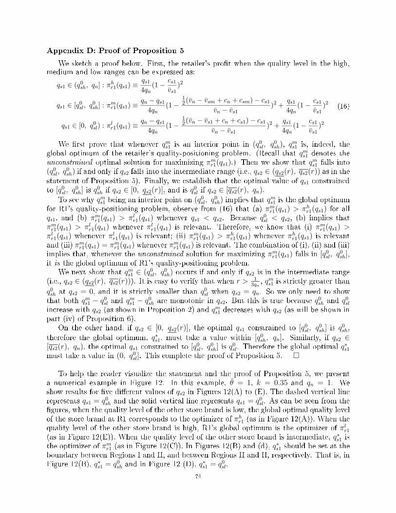
Appendix D: Proof of Proposition 5

We sketch a proof below. First, the retailer's pro�t when the quality level in the high,medium and low ranges can be expressed as:

qs1 ∈ (q0sh, qn] : πhr1(qs1) ≡

qs14qn

(1− cs1vs1

)2

qs1 ∈ [q0sl, q0sh] : πmr1(qs1) ≡

qn − qs14qn

(1−12(vn − vsm + cn + csm)− cs1

vn − vs1)2 +

qs14qn

(1− cs1vs1

)2

qs1 ∈ [0, q0sl) : πlr1(qs1) ≡

qn − qs14qn

(1−12(vn − vs1 + cn + cs1)− cs1

vn − vs1)2 +

qs14qn

(1− cs1vs1

)2

(16)

We �rst prove that whenever qms1 is an interior point in (q0sl, q0sh), qms1 is, indeed, the

global optimum of the retailer's quality-positioning problem. (Recall that qms1 denotes theunconstrained optimal solution for maximizing πm

r1(qs1).) Then we show that qms1 falls into(q0sl, q

0sh) if and only if qs2 falls into the intermediate range (i.e., qs2 ∈ (qs2(r), qs2(r)) as in the

statement of Proposition 5). Finally, we establish that the optimal value of qs1 constrainedto [q0sl, q0sh] is q

0sh if qs2 ∈ [0, qs2(r)], and is q0sl if qs2 ∈ [qs2(r), qn).

To see why qms1 being an interior point on (q0sl, q0sh) implies that q

ms1 is the global optimum

for R1's quality-positioning problem, observe from (16) that (a) πmr1(qs1) > πh

r1(qs1) for allqs1, and (b) πm

r1(qs1) > πlr1(qs1) whenever qs1 < qs2. Because q0sl < qs2, (b) implies that

πmr1(qs1) > πl

r1(qs1) whenever πlr1(qs1) is relevant. Therefore, we know that (i) πm

r1(qs1) >πlr1(qs1) whenever πl

r1(qs1) is relevant; (ii) πmr1(qs1) > πh

r1(qs1) whenever πhr1(qs1) is relevant

and (iii) πmr1(qs1) = πm

r1(qs1) whenever πmr1(qs1) is relevant. The combination of (i), (ii) and (iii)

implies that, whenever the unconstrained solution for maximizing πmr1(qs1) falls in [q0sl, q0sh],

it is the global optimum of R1's quality-positioning problem.We next show that qms1 ∈ (q0sl, q0sh) occurs if and only if qs2 is in the intermediate range

(i.e., qs2 ∈ (qs2(r), qs2(r))). It is easy to verify that when r > 13qn

, qms1 is strictly greater than

q0sh at qs2 = 0, and it is strictly smaller than q0sl when qs2 = qn. So we only need to showthat both qms1 − q0sl and qms1 − q0sh are monotonic in qs2. But this is true because q0sh and q0slincrease with qs2 (as shown in Proposition 2) and qms1 decreases with qs2 (as will be shown inpart (iv) of Proposition 6).

On the other hand, if qs2 ∈ [0, qs2(r)], the optimal qs1 constrained to [q0sl, q0sh] is q0sh,

therefore the global optimum, q∗s1, must take a value within [q0sh, qn]. Similarly, if qs2 ∈[qs2(r), qn), the optimal qs1 constrained to [q0sl, q0sh] is q

0sl. Therefore the global optimal q

∗s1

must take a value in (0, q0sl]. This complete the proof of Proposition 5. �

To help the reader visualize the statement and the proof of Proposition 5, we presenta numerical example in Figure 12. In this example, θ = 1, k = 0.35 and qn = 1. Weshow results for �ve di�erent values of qs2 in Figures 12(A) to (E). The dashed vertical linerepresents qs1 = q0sh and the solid vertical line represents qs1 = q0sl. As can be seen from the�gures, when the quality level of the other store brand is low, the global optimal quality levelof the store brand at R1 corresponds to the optimizer of πh

r1 (as in Figure 12(A)). When thequality level of the other store brand is high, R1's global optimum is the optimizer of πl

r1

(as in Figure 12(E)). When the quality level of the other store brand is intermediate, q∗s1 isthe optimizer of πm

r1 (as in Figure 12(C)). In Figures 12(B) and (d), q∗s1 should be set at theboundary between Regions I and II, and between Regions II and II, respectively. That is, inFigure 12(B), q∗s1 = q0sh and in Figure 12 (D), q∗s1 = q0sl.

74

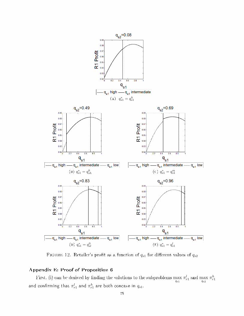
(a) q∗s1 = qhs1

(b) q∗s1 = q0sh (c) q∗s1 = qms1

(d) q∗s1 = q0sl (e) q∗s1 = qls1

Figure 12. Retailer's pro�t as a function of qs1 for di�erent values of qs2

Appendix E: Proof of Proposition 6

First, (i) can be derived by �nding the solutions to the subproblems maxqs1

πlr1 and max

qs2πhr1

and con�rming that πlr1 and πh

r1 are both concave in qs1.

75

We now prove (iv) because the result is also required in the proof of (ii). Notice that at

qms1, the sign of dqs1dqs2

is the same as the sign of ∂2πm

∂qs1∂qs2because dqs1

dqs2= −

∂∂qs2

( ∂πm∂qs1

)

∂∂qs1

( ∂πm∂qs1

)= −

∂2πm∂qs1∂qs2∂2πm∂q2s1

.

Therefore, we only need to show that at the solution to ∂πm(qs1, qs2)∂qs1

= 0, ∂2πm

∂qs1∂qs2is negative.

To facilitate the proof, we de�ne f ≡ (1− r(qn + qs1)) − qs1−qs2(qn−qs1)+(qn−qs2)

(1− r(qs1 + qs2))

and g ≡ (qn − qs1) + (qn − qs2), then after mathematical manipulations, we get

∂2πm

∂qs1∂qs2= 2qn

{∂f

∂qs2· (qn − qs1) ·

∂f

∂qs1+ f

[(qn − qs1)

∂2f

∂qs1∂qs2− ∂f

∂qs2

]}If qms1 > qs2,

∂2f∂qs1∂qs2

< 0, therefore we immediately get ∂2πm

∂qs1∂qs2< 0. If qms1 < qs2, because

(qn − qs1)∂2f

∂qs1∂qs2= −2(qs1−qs2)(1−2rqn)

g2·(1+ qn−qs2qn−qs1

)< − 2

g2(qs1 − qs2)(1 − 2rqn) (when qms1 < qs2) , we have

(qn − qs1)∂2f

∂qs1∂qs2− ∂f

∂qs2< 1

g2[2(qs2 − qs1)(1− 2rqn)− 2(qn − qs1)(1− 2rqs2)− r(qs1 − qs2)

2] =1g2[−2(qn − qs2)(1− 2rqs1)− r(qs1 − qs2)

2] < 0; therefore, we still get ∂2πm

∂qs1∂qs2< 0.

To show (ii), we only need to establish that qms1 < qhs1when qs2 = 0 because qms1 is decreasingin qs2 and qhs1 does not change with qs2. To demonstrate this, we only need to show that∂πm

r1

∂qs1< 0 at qhs1 = 1

3r. At qhs1 = 1

3r,

∂πmr1

∂qs1= qn−qs1

2f ∂f

∂qs1− 1

4f 2 + (1 − rqs1)(1 − 3rqs1) =

qn−qs12

f ∂f∂qs1

− 14f 2. Therefore we only need to con�rm that ∂f

∂qs1< 0. But when qs2 = 0, we

have ∂f∂qs1

= −r − (1−2rqs1)(2qn−qs1)+qs1(1−rqs1)(2qn−qs1)2

< 0. This shows that qms1 < qhs1 for all qs2.

We show (iii) by proving that at ql (i.e., at the unconstrained solution to maxqs1

πlr1),

∂πmr1/∂qs1 < 0. To facilitate the analysis, we further de�ne f = 1− r(qn + qs1). Then

πlr1 = 4qn

[qn − qs1

4f 2 + qs1(1− rqs1)

2

]πmr1 = 4qn

[qn − qs1

4f 2 + qs1(1− rqs1)

2

]and

∂πlr1

∂qs1= 4qn

[qn − qs1

2f∂f

∂qs1− 1

4f 2 + (1− rqs1)(1− 3rqs1)

]∂πm

r1

∂qs1= 4qn

[qn − qs1

2f∂f

∂qs1− 1

4f 2 + (1− rqs1)(1− 3rqs1)

]It is straightforward to con�rm that ∂f

∂qs1− ∂f

∂qs1= 1

g2[r · g2 + 2(qn − qs2)(1− 2rqs1)] > 0.

Therefore, if qs1 < qs2, we have f > f and f ∂f∂qs1

< f ∂f∂qs1

< 0, which then gives us∂πm

r1

∂qs1<

∂πlr1

∂qs1.

This implies that at qls1,∂πm

r1

∂qs1< 0, which then implies qms1 < qls1.

Next, we show (v). This is obvious for qls1 because qls1 =

13r. De�ne α ≡ 1

r. Then for qhs1, to

determine the sign ofdqls1dα

, we only need to determine the sign of∂2πl

r1

∂qs1∂αat qls1 because

dqs1dα

=

− ∂2πlr1

∂qs1∂α/

∂2πlr1

∂qs1∂αat qs1 = qls1. After mathematical manipulation, we get

∂2πlr1

∂qs1∂α= −8qn

α3 [34(α −

qs1)(α− 3qs1)− 2qnqs1 + q2n] +4qnα2 [

34((α− qs1) + (α− 3qs1))] =

4qnα2 [

34((α− qs1) + (α− 3qs1))]

76

at qls1. Because qls1 <13r

= α3, we have

∂2πlr1

∂qs1∂α> 0 at qls1. Therefore qls1 increases in α, which

means it decreases in r.To prove (vi), we note that

∂qms1∂ r

has the same sign as∂2πm

r1

∂qs1∂r. We have

∂2πmr1

∂qs1∂r= −8qn

g2[2qn(qn − qs1)− (qs1 + qs2) · g]

= −8qng2

[(qn − qs1) ((qn − qs1) + 2(qn − qs2))− (q2n − q2s2)

]which is negative if and only if (qn − qs1) ((qn − qs1) + 2(qn − qs2)) − (q2n − q2s2) > 0. Nowq2n−q2s2 is positive and qs1 ≤ qn so it is su�cient to show that at qn−qs1 = 0, (qn−qs1)((qn−qs1)+2(qn−qs2))−(q2n−q2s2) < 0 and when qn−qs1 = qn, (qn−qs1) ((qn − qs1) + 2(qn − qs2))−(q2n − q2s2) > 0, both of which are easy to con�rm. Therefore

∂2πmr1

∂qs1∂rmust change signs for at

some value of qs1 between zero and qn. This implies that, as qs1 increases from zero to qn,qms1 �rst decreases in r and then later increases in r.

77

CHAPTER 4

Store Brand Positioning under Various Sourcing Structures

1. Introduction

Managing store brands is very important for retailers. In 2012, store brand sales in U.S.supermarkets alone totaled $59 billion, with a store brand unit share of 23.1% and dollarshare of 19.1% (PLMA, 2013b). Retailers have spent heavily to develop their own brandsin recent years, building test kitchens, hiring culinary experts, improving packaging andtesting and retesting their products with consumers (Strom, 2013). New lines of store-brandproducts are introduced every year. For example, in 2010, Kroger more than doubled itso�erings of store-brand cosmetics and shampoos (Sewell, 2010).

Before introducing a store-brand product, the retailer needs to determine its qualitylevel. As an example, Kroger has a �three-tier� store brand positioning strategy. From theeconomy tier (i.e., the Value brand), to mid-tier store brands (such as Kroger, Ralphs andKing Soopers), to the Private Selection brand introduced in 2000, the quality level increases.Not only does Kroger need to decide the tier of a new store-brand product, but even for agiven tier, it needs to decide the quality level at a more detailed level, which would thendetermine the nature and quality of the ingredients, manufacturing processes, etc.

Some store brands are produced in-house in a manufacturing facility owned or controlledby the retailer; we call this arrangement �in-house� or IH. Some are sourced from largenational brand manufacturers who also produce and o�er competing products (�national(brand) manufacturer� or NM for short). As one example, in the UK, the large supermarketchain ASDA, has been having Coca-Cola produce its store-brand cola (Bergès-Sennou, 2006).Some are sourced from third-party manufacturers that have market power, either becauseof their overall size or because of their strength in a particular product category, and cantherefore price strategically (called �strategic (third-party) manufacturer� or SM for short).One example of a specialized store-brand manufacturer is Overhill Farms, a company knownfor making frozen foods (Choi, 2013). We note that relatively weak third-party manufacturersthat are not strategic players in their interactions with retailers can be represented in thesame way as as IH. We elaborate on this point in more detail later.

Choosing the quality level of a new store-brand product is an important strategic decisionthat the retailer is unlikely to change quickly. All of the existing literature is based on theassumption that the product is obtainable at an exogenously-speci�ed constant marginalcost. This representation is adequate if the retailer produces the product in-house or procuresit from a weak third-party producer who o�ers a �xed wholesale price (e.g., cost-plus pricing)that does not depend upon any competitive factors. Given the variety of possible sourcingarrangements and the consequent variations in pricing power among the parties, one wouldthink that the retailer's optimal choice of store brand quality should depend upon thesefactors. This is the focus of our study, and as our analysis proceeds, we show that theretailer's optimal decision di�ers markedly depending upon both the sourcing arrangementand pricing power situation.

78

More speci�cally, we study the retailer's equilibrium quality-positioning strategy underthe three sourcing structures mentioned above, and for each sourcing structure, we con-sider the three types of channel price leadership most commonly seen in the literature:Manufacturer-Stackelberg (MS), Retailer-Stackelberg (RS), and Vertical Nash (VN). Thus,we will examine nine (i.e., three times three) combinations of sourcing and pricing power (or�game�) scenarios, and compare the retailer's optimal quality positioning decision and otherequilibrium results (including prices) across the nine scenarios. In all nine combinations, theretailer moves �rst in setting the quality of her store-brand (during the product developmentphase) before any pricing decisions are made. We derive subgame perfect equilibria for allscenarios.

Typically, when a retailer is introducing a new store brand product, she has a choiceamong sources, even if she does not hold much pricing power. We build upon our analysis ofthe nine combinations of sourcing and game structure to show how the availability of othersources as outside options changes the equilibrium.

Our paper makes several contributions to the literature on store brand strategies. First,we take a �rst step in studying the interaction between store-brand sourcing and positioningdecisions, and the interplay of these decisions with the retailer's pricing power. From acomparison of the retailer's equilibrium store brand quality levels for the nine combinations ofsourcing and game structure, we obtain a full characterization of the ordering of store-brandquality level, retailer's pro�t, retail prices and consumer welfare across the nine combinations.To the best of our knowledge, we are the �rst to present a comparison of equilibria for thesenine realistic combinations of sourcing and pricing power in the store brand context. Second,we show that sourcing of store brands plays a key role in the interactions between a retailerand a national brand manufacturer. Whereas the marketing and economics literatures haveemphasized the role of store brands in helping retailers elicit price concessions from nationalbrand manufacturers, we �nd that having a preferable sourcing arrangement for a storebrand product is more valuable than having pricing power.

Our results also show that having a store brand product provides a retailer no additionalleverage in dealing with the national band manufacturer if the retailer sells the nationalbrand product and sources the store brand from the national brand manufacturer. This is incontrast to the vast majority of the literature on store-brand introduction, which concludesthat a retailer can use her store brand as a bargaining chip and thereby elicit price concessionfrom the national brand manufacturer. Finally, for two common scenarios, we show how theequilibrium�both the retailer's optimal store brand quality level and his pro�t� are a�ectedby the retailer's outside option of an alternate sourcing arrangement.

The remainder of this paper is organized as follows. In Section 2, we review the literaturethat is pertinent to our research. In Section 3, derive and compare the equilibria for thenine combinations of sourcing and game structures mentioned above. In Section 4, for twocommon scenarios, we investigate how the equilibrium is a�ected by the retailer's outsideoption vis-a-vis sourcing. In Section 5, we discuss the relationship between the results in ourpaper and those on outsourcing in similar contexts. We also discuss how supply chain pro�tdi�ers across the nine scenario. Section 6 concludes the paper.

2. Related Literature

In this literature review, we �rst brie�y discuss papers that investigate reasons why andconditions under which retailers introduce store brands. Then we review papers studying

79

store-brand positioning. We then discuss the literature on issues surrounding store brandsourcing. Finally, we discuss the only model of which we are aware that investigates chan-nel competition under di�erent price leadership structures when store brands and nationalbrands compete.

We concentrate on analytical papers, but also review a few empirical papers whose resultsare pertinent to the development of our models. For more extensive reviews on store brandstrategies, we refer readers to the book by Kumar and Steenkamp (2007), the review bySethuraman (2009) and the literature review in Chapter 2.

A major stream within the analytical literature on store brands investigates why a mo-nopolist retailer would introduce store brands. In this stream, the most well-accepted resultis that introducing a store brand (or having the option of introducing a store brand) helps aretailer elicit price concessions from upstream national brand manufacturers. In this stream,the models either do not incorporate store brand quality explicitly, or simply assume the storebrand quality level to be exogenous. Also, the models are based on the assumption of a con-stant marginal production cost for the store brand which is una�ected by the quality. Morespeci�cally, Mills (1995, 1999) under the same assumptions about demand as in our model,�nds that the wholesale price set by the national brand manufacturer is non-increasing inthe store brand quality We �nd that Mills' result depends heavily on his assumption thatthe store brand in his model is not supplied by the national brand manufacturer. In ourmodel, when the retailer sources the store brand from the national brand manufacturer, thenational brand manufacturer does not change his wholesale price for the national brand asstore brand quality increases.

Narasimhan and Wilcox (1998) and Gabrielsen and Sørgard (2007) segment customersinto those who only consider purchasing the national brand and those who consider bothbrands (�switchers�). Narasimhan and Wilcox �nd that if the number of switchers is large,the national brand manufacturer will reduce his wholesale price upon introduction of a storebrand. Gabrielsen and Sorgard allow the national brand manufacturer to condition hiswholesale price on whether the store brand is introduced. They �nd that, if the number ofswitchers is large, the national brand manufacturer will reduce its wholesale price in order toprevent the retailer from introducing the store brand. We �nd that if the retailer carries thenational brand product and outsources production of its store brand product to the nationalbrand manufacturer, the retailer is unable to elicit any price reductions, irrespective of thequality of the store brand product.

Other papers studying reasons why retailers introduce store brands have di�erent foci(and are less relevant to our research). Some focus on the role store brands play in coor-dinating a supply chain consisting of a national brand manufacturer and a retailer (Kurataet al. 2007, Colangelo 2008, Chen et al. 2011); some focus on retailers' store-brand assort-ment decisions, including the option not to o�er the national brand product (Fang et al.2012, Moner-Colonques et al. 2011, and Chapter 2 of this dissertation); some focus on theimpact of retail competition on the retailer's store brand introduction decisions (Lal andNarasimhan 1996, Corstjens and Lal 2000, Geylani et al. 2009, Groznik and Heese 2010).

Analytical papers on store-brand positioning when the store brand competes againstone or more national brands can be divided into two groups. Articles in the �rst (andlarger) group generally o�er the conclusion that store brands should seek minimal qualitydi�erentiation from the national brand(s), while articles in the other group o�er di�erentconclusions. We now discuss papers in the �rst group, followed by papers that falls into the

80

second. All of the papers discussed here are based on the assumption that the retailer andthe national brand manufacturer(s) engage in a manufacturer-Stackelberg (MS) game afterthe retailer makes the store-brand quality decision.

We �rst discuss papers whose results support minimal di�erentiation from the nationalbrand product. Sayman et al. (2002), Scott-Morton and Zettelmeyer (2004), Choi andCoughlan (2006) and Fousekis (2010) conclude that store brands should seek minimal qualitydi�erentiation from the national brand. Fousekis assumes the unit production cost of storebrand to be linearly increasing in the product quality, whereas all other authors assumethe unit production cost to be zero or constant (and therefore not a�ected by the qualitylevel). Sayman, Scott-Morton and Zettelmeyer, and Choi and Coughlan all study a retailer'sproblem of positioning a store brand against two national brands. Sayman assumes lineardemand functions and poses the retailer's quality positioning problem as one of choosingtwo parameters corresponding to the price sensitivity between the store brand and each ofthe national brands, respectively. Scott-Morton and Zettelmeyer assume the two existingnational brands are targeted at distinct customer segments. The retailer needs to eliminateone national brand if she decides to introduce the store brand. Both Sayman and Scott-Morton and Zettelmeyer show that the retailer has an incentive to position its store brandas close to the leading national brand as possible because doing so increases her bargainingpower versus the national brand. Choi and Coughlan study a retailer's problem of positioninga store brand against two national brands in both the quality and the feature dimensions.They assume a linear demand function, parameterized by the quality levels of the threeproducts and the degree of substitutability between each pair of them. The authors �nd thatthe retailer should maximize the quality level of its store brand. They also report results onstore brand positioning in the feature dimension. Fousekis (2010) studies a game in whicha national brand manufacturer and a retailer simultaneously choose the quality levels ofthe national and the store brand products, respectively, before a manufacturer-Stackelbergpricing game takes place. They �nd that the national brand manufacturer chooses thehighest quality level for the national brand irrespective of the choice of quality level madeby the retailer. The retailer also chooses the highest possible quality level for all levels ofthe national brand quality (but always smaller than the national brand quality, as assumedin their model). This implies that both the retailer and the national brand manufacturerchoose the highest quality level for their products, implying that the retailer seeks minimalquality di�erentiation from the national brand and the national brand manufacturer seeksmaximal quality di�erentiation from the store brand.

We now discuss the second group of articles on store-brand positioning. Both Du et al.(2005) and Sethuraman (2002) assume the marginal cost of production to be constant andindependent of the quality level of the product. Du et al. (2005) study an extension of ScottMorton and Scott-Morton and Zettelmeyer (2004) model with a more general representationof customer heterogeneity. They describe scenarios in which the retailer should positionthe store brand close to the weaker national brand or in between the two national brands.Sethuraman (2002) studies a game between a national brand manufacturer and one retailerin which the retailer �rst decides the quality of the store brand, then the national brand man-ufacturer sets an investment level for advertising (which will increase customers' reservationprices for products in the category). Following this, the parties engage in a manufacturer-Stackelberg pricing game. They �nd that positioning a store brand close to the nationalbrand may not be pro�table if the manufacturer can signi�cantly increase category demand

81

via advertising, or if a signi�cant portion of the market consists of consumers with low reser-vation prices who are unwilling to pay for the national brand. Bontems et al. (1999) alsostudy the store brand positioning problem by modeling a manufacturer-Stackelberg game be-tween a national brand manufacturer and a retailer. The authors assume the retailer incursa unit cost which is convex and increasing in the quality of the store brand, and identify twotypes of e�ects of increasing store brand quality: the retailer is able to get a lower wholesaleprice from the national brand manufacturer but the store brand is less competitive due toits increased marginal cost. They conclude that it is not always optimal for a retailer toposition its store brand close to the leading national brand. The authors do not report anyanalytical results on optimal store brand quality.

The academic literature on store-brand sourcing choices by retailers is sparse. The onlypaper of which we are aware on this topic is by Bergès-Sennou (2006). In this paper, tworetailers carry a national-brand product produced by a national brand manufacturer. Onlyone of the retailers has the option of carrying a store brand, whose quality level is �xed.This retailer needs to choose between producing the store brand in-house and outsourcingproduction to the national brand manufacturer, which can produce the store brand at alower unit production cost. There are four customer segments, and customers within asegment are homogenous. The �rst segment only considers buying the national brand atthe retailer without a store brand. The second segment only considers buying the storebrand from the retailer that carries a store brand. The third segment buys either the storebrand or the national brand at the retailer with a store brand, whichever provides them ahigher surplus, and the fourth segment considers buying all three products, choosing theproduct that provides them the highest surplus. The retailer with the option to o�er a storebrand �rst decides the store-brand sourcing. Then, she and the national brand manufacturernegotiate over the wholesale price for the national brand (and the store brand, if applicable),and a franchise fee, assuming an axiomatic Nash bargaining framework. If the parties failto reach an agreement after negotiating, the retailer will not sell any product(s) producedby the national brand manufacturer. Not surprisingly, the authors �nd that the retailer willentrust store brand production to the national brand manufacturer if the bargaining powerof the national brand manufacturer is below a threshold.

Finally, we brie�y review models investigating channel competition under di�erent priceleadership structures, with an emphasis on models that include store-brand products. Thereare many analytical models of traditional vertical interactions between manufacturers andretailers (e.g., McGuire and Staelin 1983, Shugan 1985, Moorthy and Fader 2012, Choi 1991,Lee and Staelin 1997). There is substantial empirical research on the nature of competitionbetween store and national brands in the presence of store brands, which suggests thatthe type of interaction and the degree of competition between national and store brandsis idiosyncratic across categories. See Putsis and Dhar (1998), Cotterill and Putsis (2000),Sayman et al. (2002), Meza and Sudhir (2010), Dhar and Ray (2004) and the referencestherein.

We are aware of only one paper that speci�cally studies the e�ect of di�erent price lead-ership structures in the context of store-national brand competition. Choi and Fredj (2013)study a game between a national brand manufacturer and two retailers. Each retailer of-fers the national brand and a store brand of their own. The store brands are assumed tohave a �xed quality level, and each retailer incurs zero marginal cost for their own storebrand. The national brand manufacturer is also assumed to incur zero marginal cost for

82

the national brand. They assume linear demand functions, in which there are two param-eters capturing the price substitutability between (1) the national brand at the two stores,and (2) the national brand and the store brand at each store. The authors compare theequilibrium outcomes among four types of games with di�erent price leadership structures:Manufacturer-Stackelberg, Retailer-Stackelberg, Vertical Nash and Retailer Double Stackel-berg. The authors show that each party earns more pro�t by having price leadership. Viasensitivity analysis on the substitubility factors in the demand functions, they show thateach retailer should seek minimum di�erentiation between their own store brand and thenational brand (in order to achieve a high demand level).

3. Quality Positioning under Various Sourcing Structures

We study games between (among) a retailer, a national brand manufacturer and a strate-gic third-party manufacturer, where applicable. The retailer carries a product (with a �xed,high quality) o�ered by the national brand manufacturer, and is considering introducing astore brand whose quality can be decided. The retailer also chooses retail prices. We de-rive and compare the retailer's equilibrium store-brand quality levels under three sourcingarrangements and three pricing power scenarios. As discussed in the Introduction, the threesources are in-house (IH), a leading national brand manufacturer (NM) whose product theretailer also carries, and a strategic third-party manufacturer (SM). The three power sce-narios are the ones most commonly seen in the literature: Manufacturer-Stackelberg (MS),Retailer-Stackelberg (RS), and Vertical Nash (VN).

Under MS with store-brand production in-house, NM �rst sets the national-brand whole-sale price, and then the retailer sets retail prices for both the national and the store brands.At this step, if the retailer decides to not introduce the store brand, she sets the retail pricefor the store brand high enough to drive demand to zero. In this way, we can implicitlymodel the store-brand introduction decision via the retailer's pricing decision. Under MSwith store-brand production by NM, NM sets the wholesale prices for both the store andnational brands, and the retailer then sets retail prices. Under MS with store-brand pro-duction by SM, NM and SM engage in a Nash game to set wholesale prices for the nationaland store brands, respectively, and the retailer then sets retail prices. Under RS, the retailersets her margins on the two products before the manufacturer(s) set their wholesale prices.Under VN, the retailer and the manufacturer(s) engage in a Nash game in which the retailersets her margins while the manufacturer(s) set the wholesale prices. In sum, we examinenine (i.e., 3 x 3) combinations of sourcing and pricing power (or �game�) scenarios, andcompare the retailer's optimal quality level and other equilibrium results (including prices)across the nine scenarios. In all nine scenarios, the retailer moves �rst in setting the qualityof her store-brand (during the product development phase) before any pricing decisions aremade, and, after all pricing decisions are made, customers make purchases. We seek subgameperfect equilibria.

Customers are heterogeneous in their willingness-to-pay (WTP) per unit of quality, whichis denoted by the parameter θ. We assume θ has a uniform distribution between 0 and θ.The utility a customer derives from either product equals her WTP per unit of qualitytimes the product quality. Each customer chooses the product that gives her the greatestsurplus (utility less price), provided that it is non-negative. We denote the quality levelof the national brand by qn, the quality level of the store brand by qs, the retail price ofthe national brand by pn and the retail price of the store brand by ps. Thus, a customer

83

with WTP for quality θ derives surplus θqn − pn from purchasing the national brand orθqs − ps from purchasing the store brand. She purchases the national brand if and onlyif θqn − pn ≥ max{θqs − ps, 0} and purchases the store brand if and only if θqs − ps ≥max{θqn−pn, 0}. Therefore, given the retail prices and the quality levels of the two products,customer demand for the store brand is Ds(pn, ps) = max{1

θ[pn−psqn−qs

− psqs], 0} and customer

demand for the national brand is Dn(pn, ps) = max{1θ[θ− pn−ps

qn−qs], 0}. We assume the quality

level of the store brand does not exceed qn. This assumption applies to the majority ofthe store brand products except for those which are called �premium store brands.� In ourmodel, this assumption is captured implicitly: the utility provided to consumers less the unitproduction cost of the store brand is decreasing in the product quality for qs > qn, so theretailer has no incentive to choose qs above this threshold.

We assume that each product has a unit production cost which is strictly convex andincreasing in the quality level. This cost relationship is applicable in settings where increas-ingly higher quality require increasingly rarer input materials, skill or processes to producethe product. Many consumer-packaged goods fall into this category. We also assume the na-tional and store brands share the same production cost function, and that the cost functionis identical across the nine scenarios studied. In reality, the national brand and third-partymanufacturers can sometimes produce the store brand at a lower unit production cost due toeconomies of scale or skill specialization. However, some major retailers have also investedheavily in their own production facilities and have strengthened their own production capa-bilities. Although they may still not be able to achieve the same level production e�ciencyas a NM or SM, the di�erence in the total variable cost (production plus transportation) perunit is likely to be small, especially when the cost of transportation to the retail stores isconsidered, as retailers tend to locate their manufacturing facilities close to the bulk of theirstore locations, whereas national brand manufacturers cannot locate their manufacturingfacilities close to every retail chain.

We denote the production cost of product x (x = s or n, denoting store and the nationalbrand respectively) as cx = C(qx), where C(·) is a convex and increasing function. For ease ofanalysis, we assume C(qx) = kq2x, where k is the production cost parameter. We also assume

that k ≤ θ2qn

, so that the �e�ciency� of producing a product (maximum utility provided to a

consumer less production cost) increases with the product quality within the interval [0, qn].This is a mild assumption that ensures sensible equilibria. If the e�ciency of producing aproduct is decreasing with the product quality, the retailer will set its quality level at zero.If the e�ciency of producing a product is �rst increasing with the product quality within[0, q′n] and then decreasing within (q′n, qn] for some q

′n < qn, the national brand manufacturer

would have an incentive to lower the quality of the national brand below qn. In our model, weassume the quality of the national brand product is �xed at qn, and our assumption ensuresthat this exogenous choice would also be incentive compatible if the choice were endogenized.

The remainder of this section is organized as follows. In Sections 3.1.1 through 3.1.3, wewe provide a detailed analysis of each party's decision problem and the equilibria under theMS game structure for sourcing under IH, SM, and NM, respectively. Next, in Section 3.1.4,we compare equilibrium quality and pro�t levels for these three scenarios. Then, in Section3.2, we present equilibria under the three sourcing structures under RS. In Section 3.3, wepresent equilibrium outcomes under all three sourcing structures under VN. We present onlysummaries of the equilibria for RS and VN; details appear in Appendix F. In Section 3.4, weprovide a comparison of equilibrium quality levels, pro�t levels, and consumer welfare across

84

all nine scenarios. Throughout the analysis, we use qn and qs to denote quality levels, wn andws to denote wholesale prices, pn and ps to denote retail prices, and, mn and ms to denoteretail margins, for the national and the store brands. respectively, where the superscript sdenotes the store brand and n denotes the national brand. Throughout most of the analysiswe omit the sourcing and game structures in the notation when this information is clearfrom the context.

3.1. Quality-positioning for the Three Sourcing Arrangements under MS

3.1.1. Quality Positioning under IH+MS

Given a wholesale price wn for the national brand product, for any store brand qualitylevel, qs, the retailer chooses retail prices to maximize pro�t:

maxps,pn

(pn − wn)Dn(pn, ps; qs) + (ps − C(qs)))Ds(pn, ps; qs) (1)

If wn < C(qs) + θ(qn − qs) and wn > C(qs)qs

qn, i.e., if the wholesale price is between lower and

upper threshold values, the retailer sells both products, setting pn(wn) =12(θqn + wn) and

ps(qs) =12(θqs + C(qs)). If wn ≥ C(qs) + θ(qn − qs), the retailer sells only her store brand.

If wn > C(qs)qs

qn, the retailer sells only the national brand.For any store brand quality level qs, the national brand manufacturer solves the following

problem to maximize his pro�t, taking into account the retailer's price reaction:

maxwn

(wn − cn) ·Dn(pn(wn), ps(qs); qs) (2)

Setting the �rst derivative with respect to wn equal to zero and con�rming concavity of theobjective function, we obtain wn(qs) =

12[θqn + cn − (θqs −C(qs))]. Because k ≤ θ

2qn, we can

verify that wn(qs) satis�es the conditions under which the retailer sells both products.Taking NM's wholesale pricing strategy into account, the retailer solves the following

quality-setting problem.

maxqs∈[0, qn]

πr(qs) ≡ [pn (wn(qs))− wn(qs)]Dn [pn (wn(qs)) , ps (qs) ; qs]

+ [ps (qs)− C(qs)]Ds [pn (wn(qs)) , ps (qs) ; qs](3)

Substituting for wn(qs), pn(wn), ps(qs) and the demand functions in πr(qs), we obtain πr(qs) =1

16θ[k2(q3n + q2nqs − qnq

2s +3q3s)− 2k(q2n +3q2s)θ+(qn +3qs)θ

2]. Therefore ∂πr(qs)∂qs

= 116θ

[9k2q2s −(2kqn + 12θ)kqs + (3θ2 + k2q2n)]. Solving ∂πr(qs)

∂qs= 0 and verifying that the solution is a

global maximum, we obtain the optimal quality level under IH+MS as min{qn, 19k[kqn +

6θ −√

−8k2q2n + 12kqnθ + 9θ2]}. The retailer never �nds it optimal to set the quality levelabove qn, because the only way this could happen is if the national brand manufacturerdecreases the national brand wholesale price below C(qs) + θ(qn − qs) which is less than itsproduction cost when qs > qn. The retailer therefore sells only the store brand, in which caseshe also has no incentive to set qs above qn because the utility provided to consumers lessthe unit production cost of the store brand is decreasing in the product quality for qs > qn.

85

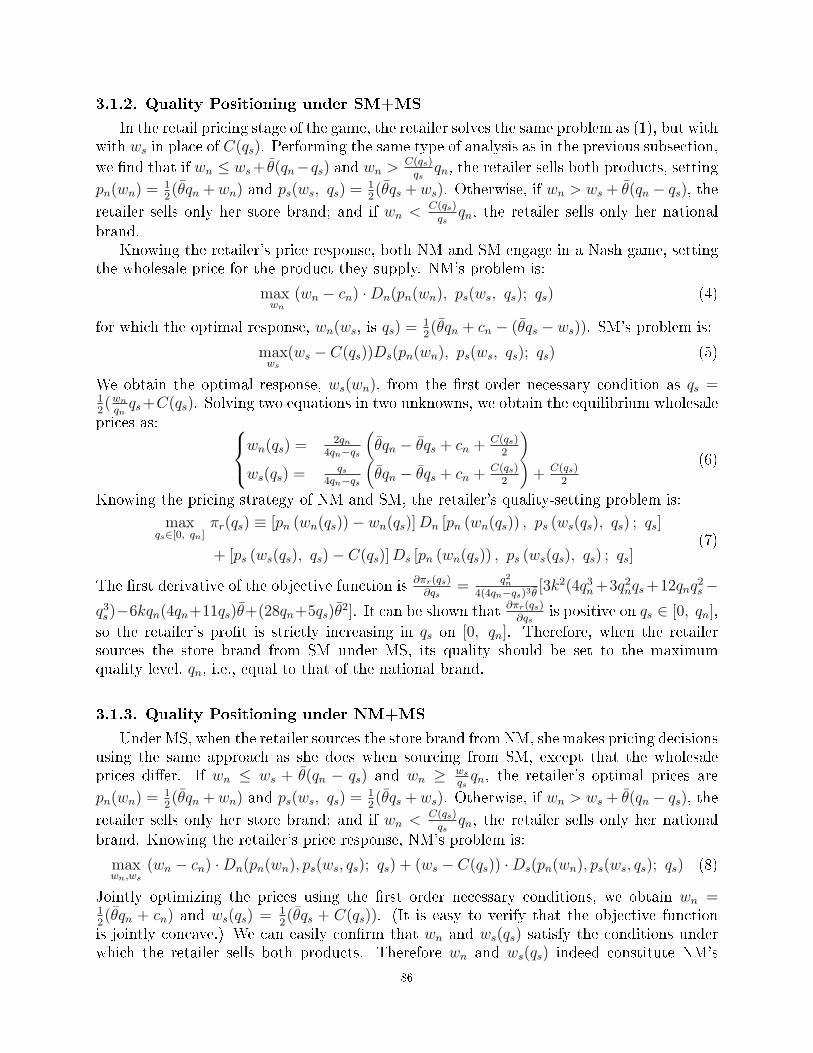
3.1.2. Quality Positioning under SM+MS

In the retail pricing stage of the game, the retailer solves the same problem as (1), but withwith ws in place of C(qs). Performing the same type of analysis as in the previous subsection,

we �nd that if wn ≤ ws+ θ(qn−qs) and wn > C(qs)qs

qn, the retailer sells both products, setting

pn(wn) =12(θqn +wn) and ps(ws, qs) =

12(θqs +ws). Otherwise, if wn > ws + θ(qn − qs), the

retailer sells only her store brand; and if wn < C(qs)qs

qn, the retailer sells only her nationalbrand.

Knowing the retailer's price response, both NM and SM engage in a Nash game, settingthe wholesale price for the product they supply. NM's problem is:

maxwn

(wn − cn) ·Dn(pn(wn), ps(ws, qs); qs) (4)

for which the optimal response, wn(ws, is qs) =12(θqn + cn − (θqs − ws)). SM's problem is:

maxws

(ws − C(qs))Ds(pn(wn), ps(ws, qs); qs) (5)

We obtain the optimal response, ws(wn), from the �rst-order necessary condition as qs =12(wn

qnqs+C(qs). Solving two equations in two unknowns, we obtain the equilibrium wholesale

prices as: wn(qs) =2qn

4qn−qs

(θqn − θqs + cn +

C(qs)2

)ws(qs) =

qs4qn−qs

(θqn − θqs + cn +

C(qs)2

)+ C(qs)

2

(6)

Knowing the pricing strategy of NM and SM, the retailer's quality-setting problem is:

maxqs∈[0, qn]

πr(qs) ≡ [pn (wn(qs))− wn(qs)]Dn [pn (wn(qs)) , ps (ws(qs), qs) ; qs]

+ [ps (ws(qs), qs)− C(qs)]Ds [pn (wn(qs)) , ps (ws(qs), qs) ; qs](7)

The �rst derivative of the objective function is ∂πr(qs)∂qs

= q2n4(4qn−qs)3θ

[3k2(4q3n+3q2nqs+12qnq2s −

q3s)−6kqn(4qn+11qs)θ+(28qn+5qs)θ2]. It can be shown that ∂πr(qs)

∂qsis positive on qs ∈ [0, qn],

so the retailer's pro�t is strictly increasing in qs on [0, qn]. Therefore, when the retailersources the store brand from SM under MS, its quality should be set to the maximumquality level, qn, i.e., equal to that of the national brand.

3.1.3. Quality Positioning under NM+MS

Under MS, when the retailer sources the store brand from NM, she makes pricing decisionsusing the same approach as she does when sourcing from SM, except that the wholesaleprices di�er. If wn ≤ ws + θ(qn − qs) and wn ≥ ws

qsqn, the retailer's optimal prices are

pn(wn) =12(θqn +wn) and ps(ws, qs) =

12(θqs +ws). Otherwise, if wn > ws + θ(qn − qs), the

retailer sells only her store brand; and if wn < C(qs)qs

qn, the retailer sells only her nationalbrand. Knowing the retailer's price response, NM's problem is:

maxwn,ws

(wn − cn) ·Dn(pn(wn), ps(ws, qs); qs) + (ws − C(qs)) ·Ds(pn(wn), ps(ws, qs); qs) (8)

Jointly optimizing the prices using the �rst order necessary conditions, we obtain wn =12(θqn + cn) and ws(qs) = 1

2(θqs + C(qs)). (It is easy to verify that the objective function

is jointly concave.) We can easily con�rm that wn and ws(qs) satisfy the conditions underwhich the retailer sells both products. Therefore wn and ws(qs) indeed constitute NM's

86

optimal solution. Given the NM's price response, the retailer's quality-setting problem is:

maxqs∈[0, qn]

πr(qs) ≡ [pn (wn)− wn]Dn [pn (wn) , ps (ws(qs), qs) ; qs]

+ [ps (ws(qs), qs)− C(qs)]Ds [pn (wn) , ps (ws(qs), qs) ; qs](9)

The objective function can be rewritten as πr(qs) =qn16θ

[k2(q2n+ qnqs− q2s)−2kqnθ+ θ2], from

which we obtain ∂πr(qs)∂qs

= k2qn16θ

(qn − 2qs). We can con�rm that πr(qs) is concave on [0, qn].

Therefore, setting the �rst derivative of the objective function to zero, we obtain qs =12qn.

3.1.4. Comparison of Equilibria for the Three Sourcing Arrangements underMS

In this section, we compare the retailer's optimal quality level across the three sourcingstructures. We use superscripts �IH�, �SM� and �NM� to distinguish the equilibria. Our ear-lier analysis established that the retailer's optimal quality levels are qIHs = min{qn, 1

9k[kqn+

6θ −√−8k2q2n + 12kqnθ + 9θ2]}, qSMs = qn and qNM

s = 12qn. The next proposition states

how they compare.

proposition 1. Under MS, qNMs < qIHs ≤ qSMs . Moreover, the last inequality holds

strictly for all k ≥ 3−√3

4θqn.

All proofs appear in the Appendix. Before discussing the intuition behind Proposition1, we introduce the following Lemma.

Lemma 1. The optimal quality level for the store brand in a centralized supply chainconsisting of the retailer and the supplier(s) of the national and store brands (as applicable),is qn/2.

Lemma 1 states that the optimal store brand quality level in a centralized supply chain isqn2. To understand this result, notice that the quality level of the store brand has two types of

e�ects on the pro�t of the supply chain. The �rst is product di�erentiation: as qs decreases,the store brand becomes more di�erentiated from the national brand, and thus total demandincreases. The second e�ect is to increase the e�ciency of the product. (Because k ≤ θ

2qn,

the maximum utility provided a customer less production cost increases with the productquality on [0, qn]). As a result, the maximum obtainable margin on store brand increases asqs increases. The centralized decision-maker must trade o� these two e�ects; the resultingoptimal quality level is qn

2.

In addition to the two e�ects just discussed, there is a third e�ect of qs when the re-tailer either produces the store brand IH or sources it from SM: a larger qs increases theretailer's negotiating power vis-a-vis the national brand manufacturer. Due to the increasedcompetition as the retailer raises qs, the national brand manufacturer is forced to decreasethe wholesale price as if the retailer had either produced the store brand IH or sourced itfrom SM. As a result, the retailer is able to get a bigger slice of the pie when she increasesqs above the optimal quality level for the centralized supply chain. Therefore, both qIHs andqSMs are greater than qn

2. In contrast, when the retailer sources the store brand from NM,

third e�ect does not exist because NM sets a same wholesale price for the national brandirrespective of qs. As such, the retailer sets q

NMs in exactly the same way as in the centralized

supply chain.

87

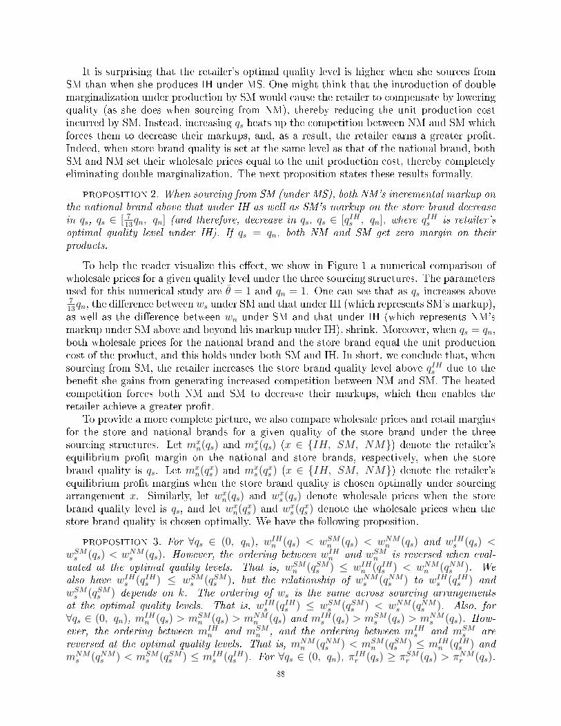
It is surprising that the retailer's optimal quality level is higher when she sources fromSM than when she produces IH under MS. One might think that the introduction of doublemarginalization under production by SM would cause the retailer to compensate by loweringquality (as she does when sourcing from NM), thereby reducing the unit production costincurred by SM. Instead, increasing qs heats up the competition between NM and SM whichforces them to decrease their markups, and, as a result, the retailer earns a greater pro�t.Indeed, when store brand quality is set at the same level as that of the national brand, bothSM and NM set their wholesale prices equal to the unit production cost, thereby completelyeliminating double marginalization. The next proposition states these results formally.

proposition 2. When sourcing from SM (under MS), both NM's incremental markup onthe national brand above that under IH as well as SM's markup on the store brand decreasein qs, qs ∈ [ 7

13qn, qn] (and therefore, decrease in qs, qs ∈ [qIHs , qn], where qIHs is retailer's

optimal quality level under IH). If qs = qn, both NM and SM get zero margin on theirproducts.

To help the reader visualize this e�ect, we show in Figure 1 a numerical comparison ofwholesale prices for a given quality level under the three sourcing structures. The parametersused for this numerical study are θ = 1 and qn = 1. One can see that as qs increases above713qn, the di�erence between ws under SM and that under IH (which represents SM's markup),

as well as the di�erence between wn under SM and that under IH (which represents NM'smarkup under SM above and beyond his markup under IH), shrink. Moreover, when qs = qn,both wholesale prices for the national brand and the store brand equal the unit productioncost of the product, and this holds under both SM and IH. In short, we conclude that, whensourcing from SM, the retailer increases the store brand quality level above qIHs due to thebene�t she gains from generating increased competition between NM and SM. The heatedcompetition forces both NM and SM to decrease their markups, which then enables theretailer achieve a greater pro�t.

To provide a more complete picture, we also compare wholesale prices and retail marginsfor the store and national brands for a given quality of the store brand under the threesourcing structures. Let mx

n(qs) and mxs(qs) (x ∈ {IH, SM, NM}) denote the retailer's

equilibrium pro�t margin on the national and store brands, respectively, when the storebrand quality is qs. Let mx

n(qxs ) and mx

s(qxs ) (x ∈ {IH, SM, NM}) denote the retailer's

equilibrium pro�t margins when the store brand quality is chosen optimally under sourcingarrangement x. Similarly, let wx

n(qs) and wxs (qs) denote wholesale prices when the store

brand quality level is qs, and let wxn(q

xs ) and wx

s (qxs ) denote the wholesale prices when the

store brand quality is chosen optimally. We have the following proposition.

proposition 3. For ∀qs ∈ (0, qn), wIHn (qs) < wSM

n (qs) < wNMn (qs) and wIH

s (qs) <wSM

s (qs) < wNMs (qs). However, the ordering between wIH

n and wSMn is reversed when eval-

uated at the optimal quality levels. That is, wSMn (qSMs ) ≤ wIH

n (qIHs ) < wNMn (qNM

s ). Wealso have wIH

s (qIHs ) ≤ wSMs (qSMs ), but the relationship of wNM

s (qNMs ) to wIH

s (qIHs ) andwSM

s (qSMs ) depends on k. The ordering of ws is the same across sourcing arrangementsat the optimal quality levels. That is, wIH

s (qIHs ) ≤ wSMs (qSMs ) < wNM

s (qNMs ). Also, for

∀qs ∈ (0, qn), mIHn (qs) > mSM

n (qs) > mNMn (qs) and mIH

s (qs) > mSMs (qs) > mNM

s (qs). How-ever, the ordering between mIH

n and mSMn , and the ordering between mIH

s and mSMs are

reversed at the optimal quality levels. That is, mNMn (qNM

s ) < mSMn (qSMs ) ≤ mIH

n (qIHs ) andmNM

s (qNMs ) < mSM

s (qSMs ) ≤ mIHs (qIHs ). For ∀qs ∈ (0, qn), π

IHr (qs) ≥ πSM

r (qs) > πNMr (qs).

88

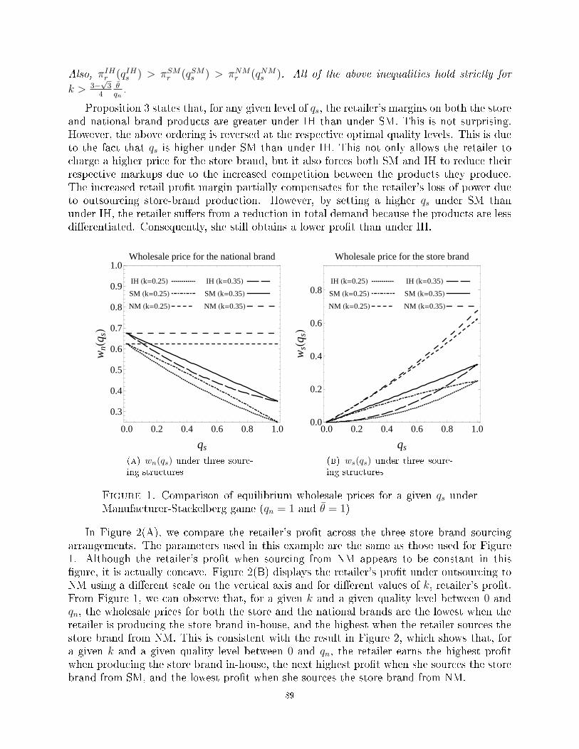
Also, πIHr (qIHs ) > πSM

r (qSMs ) > πNMr (qNM

s ). All of the above inequalities hold strictly for

k > 3−√3

4θqn.

Proposition 3 states that, for any given level of qs, the retailer's margins on both the storeand national brand products are greater under IH than under SM. This is not surprising.However, the above ordering is reversed at the respective optimal quality levels. This is dueto the fact that qs is higher under SM than under IH. This not only allows the retailer tocharge a higher price for the store brand, but it also forces both SM and IH to reduce theirrespective markups due to the increased competition between the products they produce.The increased retail pro�t margin partially compensates for the retailer's loss of power dueto outsourcing store-brand production. However, by setting a higher qs under SM thanunder IH, the retailer su�ers from a reduction in total demand because the products are lessdi�erentiated. Consequently, she still obtains a lower pro�t than under IH.

0.0 0.2 0.4 0.6 0.8 1.0

0.3

0.4

0.5

0.6

0.7

0.8

0.9

1.0

qs

wnH

q sL

Wholesale price for the national brand

IH Hk=0.25L

SM Hk=0.25L

NM Hk=0.25L

IH Hk=0.35L

SM Hk=0.35L

NM Hk=0.35L

(a) wn(qs) under three sourc-ing structures

0.0 0.2 0.4 0.6 0.8 1.00.0

0.2

0.4

0.6

0.8

qs

wsH

q sL

Wholesale price for the store brand

IH Hk=0.25L

SM Hk=0.25L

NM Hk=0.25L

IH Hk=0.35L

SM Hk=0.35L

NM Hk=0.35L

(b) ws(qs) under three sourc-ing structures

Figure 1. Comparison of equilibrium wholesale prices for a given qs underManufacturer-Stackelberg game (qn = 1 and θ = 1)

In Figure 2(A), we compare the retailer's pro�t across the three store brand sourcingarrangements. The parameters used in this example are the same as those used for Figure1. Although the retailer's pro�t when sourcing from NM appears to be constant in this�gure, it is actually concave. Figure 2(B) displays the retailer's pro�t under outsourcing toNM using a di�erent scale on the vertical axis and for di�erent values of k, retailer's pro�t.From Figure 1, we can observe that, for a given k and a given quality level between 0 andqn, the wholesale prices for both the store and the national brands are the lowest when theretailer is producing the store brand in-house, and the highest when the retailer sources thestore brand from NM. This is consistent with the result in Figure 2, which shows that, fora given k and a given quality level between 0 and qn, the retailer earns the highest pro�twhen producing the store brand in-house, the next highest pro�t when she sources the storebrand from SM, and the lowest pro�t when she sources the store brand from NM.

89

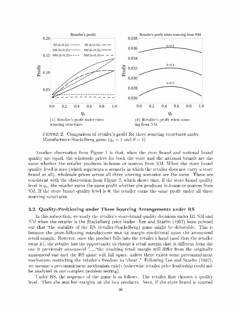
0.0 0.2 0.4 0.6 0.8 1.0

0.05

0.10

0.15

0.20

qs

Pro

fitRetailer's profit

IH Hk=0.25L

SM Hk=0.25L

NM Hk=0.25L

IH Hk=0.35L

SM Hk=0.35L

NM Hk=0.35L

(a) Retailer's pro�t under threesourcing structures

0.0 0.2 0.4 0.6 0.8 1.0

0.026

0.028

0.030

0.032

0.034

0.036

0.038

qs

Pro

fit

Retailer's profit when sourcing from NM

k=0.3

k=0.4

k=0.5

(b) Retailer's pro�t when sourc-ing from NM

Figure 2. Comparison of retailer's pro�t for three sourcing structures underManufacturer-Stackelberg game (qn = 1 and θ = 1)

Another observation from Figure 1 is that, when the store brand and national brandquality are equal, the wholesale prices for both the store and the national brands are thesame whether the retailer produces in-house or sources from SM. When the store brandquality level is zero (which represents a scenario in which the retailer does not carry a storebrand at all), wholesale prices across all three sourcing scenarios are the same. These areconsistent with the observation from Figure 2, which shows that, if the store brand qualitylevel is qn, the retailer earns the same pro�t whether she produces in-house or sources fromSM. If the store brand quality level is 0, the retailer earns the same pro�t under all threesourcing structures.

3.2. Quality-Positioning under Three Sourcing Arrangements under RS

In this subsection, we study the retailer's store-brand quality decisions under IH, SM andNM when the retailer is the Stackelberg price leader. Lee and Staelin (1997) have pointedout that �the stability of the RS (retailer-Stackelberg) game might be debatable. This isbecause the price-following manufacturer sets its margin conditional upon the announcedretail margin. However, once the product falls into the retailer's hand (and thus the retailerowns it), the retailer has the opportunity to charge a retail margin that is di�erent from theone it previously announced �.....�the resulting retail margin will di�er from the originallyannounced one and the RS game will fall apart, unless there exists some precommitmentmechanism restricting the retailer's freedom to `cheat'.� Following Lee and Staelin (1997),we assume a precommitment mechanism exists (otherwise retailer price leadership could notbe analyzed in our complex problem setting).

Under RS, the sequence of the game is as follows. The retailer �rst chooses a qualitylevel. Then she sets her margins on the two products. Next, if the store brand is sourced

90

in-house, NM sets the national-brand wholesale price. If the store brand is produced by NM,NM sets the wholesale prices for both the store and national brands. If the store brand isproduced by SM, NM and SM engage in a Nash game to set wholesale prices for the productsthey produce. Finally, customers make purchases. For brevity, we omit derivations here andrefer the reader to Appendix E for details.

proposition 4. Under RS, when the retailer produces the store brand IH, the optimalquality level for the store brand is qIHs = min{ 1

3k2[k2qn+2kθ−(−2k4q2n+4k3qnθ+k2θ2)

12 ], qn}.

When the retailer sources the store brand from SM, if k ≤ 3−√3

3θqn

≈ 0.42 θqn, the optimal

quality level for the store brand is qn, but if k ∈ [3−√3

3θqn, θ

2qn], the optimal store brand

quality, qSMs , is the smallest solution to −2k2(qSMs )3 + (13k2qn + 2kθ)(qSMs )2 − (8k2q2n +16kqnθ)q

SMs +(6k2q3n− 4kq2nθ+6qnθ

2) = 0 on (0, qn). There are three solutions to this cubic

equation. When k ≤ 3−√3

3θqn

≈ 0.42 θqn, all the three solutions are greater than qn, in which

case qn is the optimal solution. Otherwise, if k > 3−√3

3θqn, the smallest solution falls below

qn and is the optimal solution to the retailer's problem. When the retailer sources the storebrand from NM, the optimal quality is qNM

s = qn2.

We defer the comparison of qIHs , qSMs and qNMs under RS to Section 3.4. Next, we discuss

the retailer's quality setting strategy under another type of channel interaction: verticalNash.

3.3. Quality-positioning under Three Sourcing Arrangements under VN

Under our Vertical Nash pricing games, the retailer �rst chooses her store brand quality.Then, the retailer and the manufacturer(s) engage in a Nash game in which the retailer setsthe retail margins for both products, and the manufacturer(s) sets the wholesale price(s) forthe product(s) they produce. Finally, customers make purchase decisions. Below, we presentoptimal quality levels for the three sourcing arrangements under VN. We refer the reader tothe proof of Proposition 5 in Appendix F for a detailed derivations of these results.

proposition 5. Under VN, when the retailer produces the store brand IH, the optimalquality level for the store brand is qIHs = min{qn, 1

15k[4kqn + 10θ − (−44k2q2n + 80kqnθ +

25θ2)12 ]}. When the retailer sources the store brand from SM, k ≤ 17−4

√5

19θqn

≈ 0.424 θqn

the

optimal quality level for the store brand is qn . If k ∈ [17−4√5

19θqn, θ

2qn], the optimal store

brand quality, qSMs , is the smallest solution to −5k2q2n(qSMs )3 +135k2q3n(q

SMs )2 + (−32k2q4n −

218kq3nθ+7q2nθ2)qSMs +(54k2q5n− 54kq4nθ+81q3nθ

2) = 0 on (0, qn). There are three solutions

to this cubic function. When k ≤ 3−√3

3θqn

≈ 0.42 θqn, all the three solutions are greater than

qn, in which case qn is the optimal solution. Otherwise, if k > 3−√3

3θqn, the smallest solution

falls below qn and is the optimal solution to the retailer's problem. When the retailer sourcesthe store brand from NM, the optimal quality is qNM

s = qn2.

3.4. Comparison of Quality Positioning Across Nine Scenarios

We have now derived the optimal quality levels for the nine combinations of game-and-sourcing structures and can proceed to compare them. We have the following proposition.

91

proposition 6. When sourcing from NM under the three game structures, the optimalquality level is qn

2, for all three game structures, and the retailer's pro�t levels have the

ordering of MS+NM < VN+NM < RS+NM. Both the quality and pro�t levels are the lowestamong the nine combinations. For the remaining six combinations of game-and-sourcingstructures, the ordering of the retailer's optimal quality levels is MS+SM ≥ VN+SM ≥RS+SM ≥ MS+IH ≥ VN+IH ≥ RS+IH, whereas her pro�t levels are in the reverse order.Furthermore, ∃k1 ∈ (0, θ

2qn) such that, for ∀k ∈ (k1,

θ2qn

], all of the inequalities above holdstrictly.

Proposition 6 presents results on the relation among the retailer's optimal quality levelsand optimal pro�t levels across nine scenarios. We next discuss the intuition behind theseresults shortly. Before we do so, notice that from Proposition 6, if the retailer chooses theoptimal quality level for each scenario, her pro�t levels across the nine scenarios have theordering of RS + IH ≥ V N + IH ≥ MS + IH ≥ RS + SM ≥ V N + SM ≥ MS + SM >RS + NM > VN + NM > MS + NM . One might ask whether this ordering holds if theretailer does not have the �exibility to change quality levels across di�erent scenarios? Thefollowing corollary answers this question.

corollary 1. Suppose the quality level of the store brand is �xed and equal acrossscenarios. Then, given a sourcing structure, the retailer's pro�t level across the three gamestructures have the ordering of RS≥VN≥MS, with the inequality holding strictly for qs ∈(0, qn)). Given a game structure, the retailer's pro�t across the three sourcing structureshave the ordering of IH ≥ SM ≥ NM with the inequalities holding strictly for qs ∈ (0, qn)).These orderings are consistent with the ordering of optimal pro�t levels stated in Proposition6. However, di�erent from the ordering stated in Proposition 6, the retailer's pro�t levelunder MS+IH can be smaller than her pro�t under RS+SM, and the retailer's pro�t underMS+SM can be smaller than her pro�t under RS+NM. These orderings arise if qs is smallerthan a threshold.

We now discuss the intuition behind Proposition 6 and Corollary 1. Past literature onstore-brand introduction has established that introducing a store brand helps a retailer elicitprice concession from upstream NMs (Mills 1995 and 1999, Narasimhan and Wilcox 1998,Gabrielsen and Sørgard 2007, etc.). Proposition 6 states that this e�ect is not present if theretailer sources the store brand from NM, even if the retailer is the Stackelberg price leader.This occurs because if the retailer sources the store brand from NM, she confers pricingpower over the wholesale prices of both the store and national brands to NM. As a result,NM chooses the same wholesale price on the national brand product irrespective of the storebrand quality level, even if he is a Stackelberg follower when setting prices. Consequently,the retailer's only source of leverage provided by the store brand is product di�erentiation.As such, she chooses a low quality level that provides signi�cant di�erentiation from thenational brand product. The di�erentiation leads to an increase in overall pro�t for theretailer (versus having no store brand), so she adopts this low-quality choice. In this case,the retailer's optimal quality level is equal to that for the centralized supply chain consistingof the retailer and the national brand manufacturer, and the optimal quality level turns outto be lower than those in any of the other six scenarios. It appears that, in this case, theretailer is better o� trying to appeal to the portion of the market that the national brandmanufacturer cannot easily reach, rather than competing head-on with the national brandmanufacturer when he has no incentive to o�er the retailer a low price on her store brand

92

product. The retailer's resulting pro�t is also the lowest when she sources the store brandfrom NM than under any other sourcing arrangement.

Under the remaining six scenarios (i.e., under combinations involving IH or SM), the re-tailer uses the store-brand quality level more aggressively as a lever to (partially) compensatefor any reduction in leverage arising from a less advantageous sourcing arrangment or weakerpricing power. The optimal store-brand quality has a monotonic mapping to the game-and-sourcing combinations, with the optimal quality increasing along the following path: RS+IH−→VN+IH −→MS+IH −→RS+SM −→VN+SM −→MS+SM. Stated another way, the op-timal quality level for the centralized channel (consisting of the retailer and manufacturer(s))is low. But as the retailer's sourcing arrangement or pricing power becomes less advanta-geous, the retailer can wrest a larger portion of the supply chain pro�t by deviating fromthe optimal quality level for the centralized system.

As mentioned in Section 3.1.4, the retailer sets a higher quality level when sourcing fromSM than from IH under MS. We can also o�er a stronger result: the retailer sets a higherquality level under SM than under IH, even if her pricing power di�ers between the twoscenarios being compared. Surprisingly, this e�ect leads to the retailer even to choose ahigher quality level under SM when she has pricing power (i.e., under RS) than she doesunder IH when NM is the Stackelberg price leader (i.e. under MS). The main reason is thatwhen sourcing from SM, by increasing qs, the retailer can heat up the competition betweenthe national and the store brand manufacturers, which forces them to decrease their markups.This bene�t is not available under IH.

Above, we compared the retailer's optimal quality levels across the nine scenarios. Next,we discuss the intuition for results regarding the retailer's pro�t levels in Proposition 6 andCorollary 1 which state that (i) given a game structure, the retailer prefers IH over SM overNM; and (ii) given a sourcing structure, the retailer prefers RS over VN over MS. Results(i) and (ii) hold both when the retailer's store brand quality level is �xed, and when theretailer chooses an optimal quality level for each of the scenarios. Although these results areintuitive, we are (to the best of out knowledge) the �rst to formally establish comparisonacross store brand sourcing arrangements.

We note that (ii) is consistent with the past literature on the value of being a price leader.For example, Choi (1991) and Lee and Staelin (1997) �nd that if the type of interaction in achannel is such that a channel member's best response is to reduce its margin when its channelpartner increases its margin, then each channel member prefers having price leadership.This is exactly the type of channel interaction that arises in our model. In particular, ifthe national brand manufacturer experiences a cost increase (decrease) in our model andhence increases (decreases) its wholesale price, the retailer will not pass on the full amountof the change to customers. We are only aware of one paper involving store brand productsthat compares di�erent vertical price leadership structures. Choi and Fredj (2013) study theinteraction between a national brand manufacturer and two retailers (each o�ering a storebrand), and show that each party earns more pro�t by having price leadership. Because theauthors assume the retailers incur zero marginal cost on store brands, their model representsa special scenario in which the retailer produces the store brand IH and incurs no cost relatedto quality. We �nd that this result carries over to other sourcing arrangements as well. Thatis, given a sourcing structure, the retailer prefers RS over VN over MS.

We now turn to a comparison of the retailer's pro�t across scenarios when both pricingpower and sourcing structure vary. Proposition 6 states that at the optimal quality level

93

for store brand corresponding to each scenario, the retailer strictly prefers a scenario witha more preferable sourcing structure, even if she is a price follower in this scenario but aleader in the other. For example, retailer's pro�t under MS+IH is greater than her pro�tunder RS+SM. This �nding implies that, although past literature emphasizes how storebrands give a retailer more pricing power versus the national brand manufacturer, a morepreferable sourcing structure has greater value than a more favorable pricing power scenarioto the retailer, i.e., the power to choose the source is more important than than pricingpwer. One key reason for this result is that sourcing from an outside party confers powerover wholesale pricing even if that party is not the Stackelberg price leader. A less obviousreason is that sourcing from an outside party can cause the retailer to choose a lower qualityfor the store brand product than when it is produced in-house. This does occur whenthe retailer outsources to NM (but not when she outsources to SM). It is important toemphasize, however, that this result holds only when the retailer chooses the correspondingoptimal quality level for each scenario. If the store brand quality level is �xed, it is possiblethat the retailer prefers RS+SM over MS+IH, or prefers RS+NM over MS+SM. Intuitively,if the store brand quality is too low, it does not pose enough of threat to the national brandmanufacturer even if the retailer has a preferable sourcing arrangement for her store brand.In this case, the retailer does not gain much from having a preferable sourcing arrangement.Instead, she bene�ts more from having pricing leadership in the supply chain.

Next, we compare customer welfare at the optimal store brand quality levels, as well asequilibrium retail prices, across the nine combinations of game-and-sourcing structure.

proposition 7. Across the nine game-and-sourcing structures, the ordering of the con-sumer welfare is VN+IH ≥MS+IH ≥ RS+IH ≥ VN+SM ≥ MS+SM ≥ RS+SM ≥ VN+NM≥ RS+NM = MS+NM. Furthermore, ∃k2 ∈ (0, θ

2qn) such that, for ∀k ∈ (k2,

θ2qn

], all of theinequalities above hold strictly.

corollary 2. Suppose quality level of the store brand is �xed. Then, given a sourcingstructure, customer welfare across the three pricing power scenarios have the ordering ofV N ≥ MS = RS, and the inequalities hold strictly for qs ∈ (0, qn)). Given a pricing powerscenario, customer welfare across the three sourcing structures have the ordering of IH ≥SM ≥ NM and the inequalities hold strictly for qs ∈ (0, qn)). These orderings are consistentwith the ordering of the optimal quality levels stated in Proposition 7. However, di�erent fromthe ordering stated in Proposition 7, customer welfare under RS+IH can be smaller thanthat under VN+SM, and can be smaller under RS+SM than that under VN+NM. Theserelationships arise when qs is smaller than a threshold.

corollary 3. Given a sourcing structure, the qs that maximizes the retailer's pro�t un-der VN and MS also maximizes customer welfare under VN and MS, respectively. However,under RS, the retailer chooses a lower quality level than that which maximizes customerwelfare.

Proposition 7, and Corollaries 2 and 3 imply that:(i) Given a game structure, customers prefer IH over SM over NM (just as the retailer does).This result holds both when the quality level is �xed and when the retailer chooses her op-timal quality level for each scenario.(ii) When quality level is �xed and equal across scenarios, given a sourcing structure, cus-tomers prefer VN over MS or RS, and are indi�erent between MS and RS.(iii) When the retailer chooses the quality level optimally for each scenario, the quality level

94

is also optimal for consumers when the pricing scenario is VN or MS. Under RS, she choosesa quality level lower than the optimal quality level for consumers.

The combination of (ii) and (iii) implies that:(iv) when the retailer chooses her optimal quality level for each scenario, customers are bettero� under VN than they are under MS, and better o� under MS than under RS. Finally, theresults imply that:(v) when the retailer chooses her optimal quality for each scenario, customers prefer a �better�sourcing arrangement irrespective of the pricing power scenario.However, this result does not hold if the store brand quality level is �xed and equal acrossscenarios and is lower than a threshold. We elaborate each of these �ndings below.

Finding i) is consistent with the �ndings of Chen et al. (2010), who present results ofan empirical study to estimate parameters of the demand and supply functions in a modelof strategic interaction between two national brand manufacturers and two retailers for the�uid milk category in a major metropolitan area. They assume the type of competitionbetween store brands upstream to be Cournot-Nash. That is, they assume that store brandsare homogeneous at the wholesale level, producers (the national brand manufacturer andthe retailers) simultaneously choose their production quantities, and price is determined bymarket clearing. On the other hand, they assume national brand products are di�erentiatedupstream and compete in a Bertrand-Nash fashion. Downstream, all products are di�eren-tiated and compete in a Bertrand-Nash fashion. Their results indicate that consumers arebetter o� when the retailer produces the store brand in-house than when she sources thestore brand from a national brand manufacturer. This result would be expected in view ofthe e�ect of double marginalization.

Finding (ii) above is also consistent with results the literature. Choi (1991) and Leeand Staelin (1997) �nd that the equilibrium retail prices under MS and RS are the sameand are higher than the retail prices under VN. This result implies that customers strictlyprefer no channel leadership over the presence of channel leadership, and are indi�erent asto who takes channel price leadership. However, our results (iii) and (iv) state that this isnot true when the retailer chooses the optimal store brand quality level for each scenario.When she does so, the quality level she chooses under VN (MS) also maximizes consumerwelfare under VN (MS), while she chooses a quality level that is suboptimal for consumersunder RS. This means that customers strictly prefer MS over RS (even though they wouldhave secured the same welfare under the two game scenarios if the quality levels were thesame). Finally, our �nding (v) says that when the retailer chooses her quality level optimallyfor each of the nine scenarios, customers prefer a preferable sourcing structure irrespectiveof the pricing power scenario. This result contributes to the store brand literature by againsuggesting that managing sourcing is more important than gaining pricing power, because,not only the retailer, but also the customers, prefer the store brand being sourced in-house,irrespective of the pricing power scenario. However, one should understand that this resultmay not hold if the retailer does not have the �exibility to choose the optimal quality levelfor each scenario. If the quality level is lower than a threshold, the store brand does not poseenough of a threat to the national brand manufacturer, therefore a �good� sourcing structureis less valuable to both the retailer and customers.

While consumer welfare has the same ordering across the nine game-and-sourcing com-binations for all k, the ordering of equilibrium retail prices across the nine combinationsdepends on the value of k. Indeed, for a given qs ∈ (0, qn), the ordering of the equilibrium

95

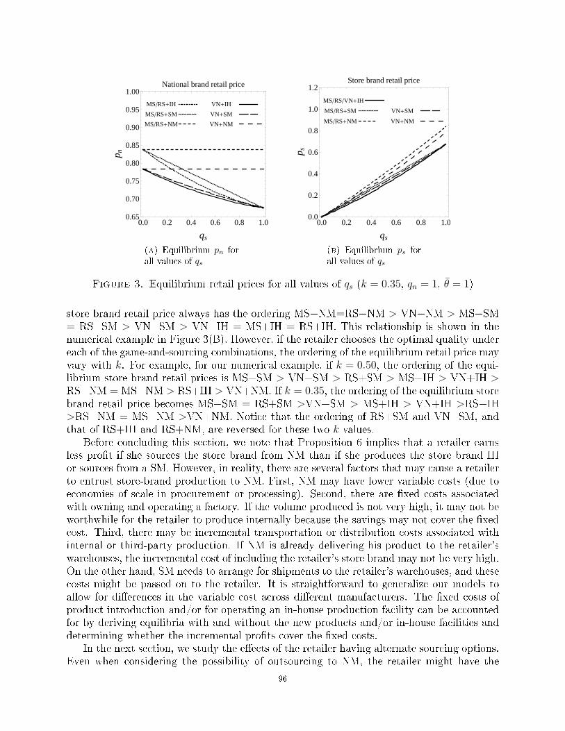
0.0 0.2 0.4 0.6 0.8 1.00.65

0.70

0.75

0.80

0.85

0.90

0.95

1.00

qs

p n

National brand retail price

MS�RS+IH

MS�RS+SM

MS�RS+NM

VN+IH

VN+SM

VN+NM

(a) Equilibrium pn forall values of qs

0.0 0.2 0.4 0.6 0.8 1.00.0

0.2

0.4

0.6

0.8

1.0

1.2

qs

p s

Store brand retail price

MS�RS�VN+IH

MS�RS+SM

MS�RS+NM

VN+SM

VN+NM

(b) Equilibrium ps forall values of qs

Figure 3. Equilibrium retail prices for all values of qs (k = 0.35, qn = 1, θ = 1)

store brand retail price always has the ordering MS+NM=RS+NM > VN+NM > MS+SM= RS+SM > VN+SM > VN+IH = MS+IH = RS+IH. This relationship is shown in thenumerical example in Figure 3(B). However, if the retailer chooses the optimal quality undereach of the game-and-sourcing combinations, the ordering of the equilibrium retail price mayvary with k. For example, for our numerical example, if k = 0.50, the ordering of the equi-librium store brand retail prices is MS+SM > VN+SM > RS+SM > MS+IH > VN+IH >RS+NM =MS+NM > RS+IH > VN+NM. If k = 0.35, the ordering of the equilibrium storebrand retail price becomes MS+SM = RS+SM >VN+SM > MS+IH > VN+IH >RS+IH>RS+NM = MS+NM >VN+NM. Notice that the ordering of RS+SM and VN+SM, andthat of RS+IH and RS+NM, are reversed for these two k values.

Before concluding this section, we note that Proposition 6 implies that a retailer earnsless pro�t if she sources the store brand from NM than if she produces the store brand IHor sources from a SM. However, in reality, there are several factors that may cause a retailerto entrust store-brand production to NM. First, NM may have lower variable costs (due toeconomies of scale in procurement or processing). Second, there are �xed costs associatedwith owning and operating a factory. If the volume produced is not very high, it may not beworthwhile for the retailer to produce internally because the savings may not cover the �xedcost. Third, there may be incremental transportation or distribution costs associated withinternal or third-party production. If NM is already delivering his product to the retailer'swarehouses, the incremental cost of including the retailer's store brand may not be very high.On the other hand, SM needs to arrange for shipments to the retailer's warehouses, and thesecosts might be passed on to the retailer. It is straightforward to generalize our models toallow for di�erences in the variable cost across di�erent manufacturers. The �xed costs ofproduct introduction and/or for operating an in-house production facility can be accountedfor by deriving equilibria with and without the new products and/or in-house facilities anddetermining whether the incremental pro�ts cover the �xed costs.

In the next section, we study the e�ects of the retailer having alternate sourcing options.Even when considering the possibility of outsourcing to NM, the retailer might have the

96

option of using a strategic third-party manufacturer or even producing in-house. We inves-tigate NM's optimal strategy under threat of the retailer choosing an alternate source, aswell as the retailer's optimal quality decisions in this environment.

4. National brand manufacturer's strategy and retailer's optimal quality levelwhen the retailer has alternate sources

In this section, we study two variants of the game between the national brand manufac-turer and the retailer. In the two variants, the retailer is asking the national brand man-ufacturer to produce both products under the implicit threat of using an alternate source,either IH or SM, to produce the store brand product. The retailer often has an alternatesource, so these games represent realistic market environments.

We next describe the sequence of decisions in these games. First, the retailer sets thestore brand quality level and asks the national brand manufacturer to quote wholesale pricesfor the national and store brand products, (wn, ws). The retailer then decides whetherto source both products from the national brand manufacturer. If she decides to do so,(wn, ws) becomes e�ective. Otherwise, the retailer can source the store brand from heralternate source, in which case she will ask the national brand manufacturer to quote awholesale price only on the national brand product. If SM is the alternate source for thestore brand product, then NM's quote is determined via a Nash pricing game between SM andNM (as in the models analyzed earlier in this paper). Finally, the retailer sets retail pricesand customer demands are realized. As before, we seek subgame-perfect Nash equilibria.We now proceed to analyze these two game variants using backward induction.

Given any qs, the national brand manufacturer solves the following problem to set thewholesale prices if he is producing both products:

maxwn, ws

πm(wn, ws) (10)

πr(wn, ws) ≥ πr0 (11)wn − ws

qn − qs≥ ws

qs(12)

cs ≤ ws ≤ wn

qnqs (13)

where, given (wn, ws) set by the national brand manufacturer, pn(wn, ws) =12(θqn + wn)

and ps(wn, ws) =12(θqs + ws) are the retailer's optimal price response, and

πm(wn, ws) ≡(wn − cn)Dn(pn(wn, ws), ps(wn, ws); qs)

+ (ws − cs)Ds(pn(wn, ws), ps(wn, ws); qs)

and

πr(wn, ws) ≡(pn(wn, ws)− wn)Dn(pn(wn, ws), ps(wn, ws); qs)

+ (ps(wn, ws)− ws)Ds(pn(wn, ws), ps(wn, ws); qs)

are NM's and retailer's pro�t respectively. De�ne πr0 in (11) as the retailer's �reservationpro�t,� which is the pro�t she would earn if she uses her alternate source to produce thestore brand. Constraint (11) is a participation constraint that ensures the national brandmanufacturer chooses wholesale prices so that the retailer earns at least her reservationpro�t. Thus, πr0 ≡ (pn(wn0, ws0) − wn0)Dn(pn(wn0, ws0), ps(wn0, ws0); qs) + (ps(wn0, ws0) −

97

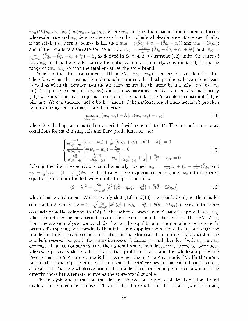
ws0)Ds(pn(wn0, ws0), ps(wn0, ws0); qs), where wn0 denotes the national brand manufacturer'swholesale price and ws0 denotes the store brand supplier's wholesale price. More speci�cally,if the retailer's alternate source is IH, then wn0 =

12(θqn + cn − (θqs − cs)) and ws0 = C(qs);

and if the retailer's alternate source is SM, wn0 = 2qn4qn−qs

(θqn − θqs + cn +

cs2

)and ws0 =

qs4qn−qs

(θqn − θqs + cn +

cs2

)+ cs

2, as derived in Section 3. Constraint (12) limits the range of

(wn, ws) so that the retailer carries the national brand. Similarly, constraint (13) limits therange of (wn, ws) so that the retailer carries the store brand.

Whether the alternate source is IH or SM, (wn0, ws0) is a feasible solution for (10).Therefore, when the national brand manufacturer supplies both products, he can do at leastas well as when the retailer uses the alternate source for the store brand. Also, because πm

in (10) is jointly concave in (wn, ws), and its unconstrained optimal solution does not satisfy(11), we know that, at the optimal solution of the manufacturer's problem, constraint (11) isbinding. We can therefore solve both variants of the national brand manufacturer's problemby maximizing an �auxiliary� pro�t function:

maxwn, ws

πm(wn, ws) + λ [πr(wn, ws)− πr0] (14)

where λ is the Lagrange multipliers associated with constraint (11). The �rst order necessaryconditions for maximizing this auxiliary pro�t function are:

λ−22θ(qn−qs)

(wn − ws) +12θ

[k(qn + qs) + θ(1− λ)

]= 0

λ−22θ(qn−qs)

( qnqsws − wn)− kqn

2θ= 0

w2n

4θ(qn−qs)+

qnqs

w2s

4θ(qn−qs)− wn

[ws

2θ(qn−qs)+ 1

2

]+ θqn

4− πr0 = 0

(15)

Solving the �rst two equations simultaneously, we get wn = 12−λ

cn + (1 − 12−λ

)θqn and

ws = 12−λ

cs + (1 − 12−λ

)θqs. Substituting these expressions for wn and ws into the thirdequation, we obtain the following implicit expression for λ:

(2− λ)2 =qn

4πr0θ

[k2

(q2n + qnqs − q2s

)+ θ(θ − 2kqn)

](16)

which has two solutions. We can verify that (12) and(13) are satis�ed only at the smaller

solution for λ, which is λ = 2−√

qn4πr0θ

[k2 (q2n + qnqs − q2s) + θ(θ − 2kqn)

]). We can therefore

conclude that the solution to (15) is the national brand manufacturer's optimal (wn, ws)when the retailer has an alternate source for the store brand, whether it is IH or SM. Also,from the above analysis, we conclude that at the equilibrium, the manufacturer is strictlybetter o� supplying both products than if he only supplies the national brand, although theretailer pro�t is the same as her reservation pro�t. Moreover, from (16), we know that as theretailer's reservation pro�t (i.e., πr0) increases, λ increases, and therefore both wn and ws

decrease. That is, not surprisingly, the national brand manufacturer is forced to lower bothwholesale prices as the retailer's reservation pro�t increases, and the wholesale prices arelower when the alternate source is IH than when the alternate source is SM. Furthermore,both of these sets of prices are lower than when the retailer does not have an alternate source,as expected. At these wholesale prices, the retailer earns the same pro�t as she would if shedirectly chose her alternate source as the store-brand supplier.

The analysis and discussion thus far in this section apply to all levels of store brandquality the retailer may choose. This includes the result that the retailer (when sourcing

98

from NM while she has an alternate source) earns the same pro�t as she would if she directlychose her alternate source. Therefore, the optimal quality level the retailer chooses, underthe modi�ed scenario discussed in this section, equals the optimal quality level she wouldchoose when using the alternate source.

corollary 4. Suppose the retailer sources both products from the national brand man-ufacturer while she has the option of using an alternate source, either IH or SM, to producethe store brand. Then the retailer makes the quality positioning decision in the same way asif she were securing the store brand from the alternate source.

Although the retailer's optimal quality is the same as if she were sourcing the store brandfrom the alternate source, the equilibrium prices are not the same in the two settings. Takingthe scenario in which the alternate source is IH as an example, when the retailer producesthe store brand in-house, the �wholesale price� for the store brand is cs and the wholesaleprice for the national brand is wn0 =

12cn +

12(θqn − (θqs − cs)). However, if the retailer were

sourcing both products from the national brand manufacturer under threat of the retailerusing IH, national brand manufacturer's wholesale prices would be wn = 1

2−λcn+(1− 1

2−λ)θqn

and ws =1

2−λcs+(1− 1

2−λ)θqs. For any given value of qs, ws is greater than cs and it is easy

to show that wn is less than wn0.Figure 4 shows the national brand manufacturer's pricing strategy and the retailer's

equilibrium pro�t for di�erent values of qs in the presence and absence of an alternate sourcefor the store brand. From the �gure, we can observe that in the presence of an alternatesource, the national brand manufacturer has an incentive to select the wholesale prices tosecure his position as the supplier of both the national and store brands. These prices arechosen so as to make the retailer indi�erent between the two sourcing options. The reasonwhy the retailer chooses the same quality level under both scenarios can be explained asfollows. Suppose the retailer's optimal quality level for the better alternate source is q. Thenational brand manufacturer has selected wholesale prices to make the retailer indi�erentbetween this option and NM, but the wholesale prices are di�erent under the two scenarios.The question is whether the retailer can improve her pro�t by choosing q = q given thewholesale prices selected by NM. We claim that the retailer cannot do so. The logic is asfollows. If the retailer could improve her pro�t by choosing q = q when sourcing the storebrand from NM, then she could also improve her pro�t by choosing q = q when sourcing fromher alternate source, as the retailer is indi�erent between sourcing from NM and sourcingfrom her alternate source (for all values of store brand quality). But this contradicts theoptimality of choosing q when the retailer is sourcing from her alternate source. In the proofof Corollary 4 (see Appendix I), we show that the retailer cannot increase her pro�t bydeviating from q even though the wholesale prices are di�erent under the two scenarios.

That the retailer is made indi�erent between di�erent sourcing structures under themodi�ed scenario studied in this section partly explains why di�erent retailers source storebrand products in di�erent ways, and a given retailer often sources the store brand di�erentlyfor di�erent categories of products. Indeed, the landscape of store-brand production has beenchanging. For example, Kroger has been attempting to purchase manufacturing capacity toproduce more store-brand products in-house (Chen, 2010). Safeway, on the other hand,recently sold one of its manufacturing plants to a third-party manufacturer that will takeover production of some of its store-brand products (Annie's, Inc., 2013). Moreover, whilethe store brand quality should be set di�erently under di�erent sourcing structures when

99

retailer does not have easy access to an alternate source, this is not true when she has suchan option, in which case the retailer would set the quality level equal to the optimal qualitylevel for the best of the available sourcing options.

0.0 0.2 0.4 0.6 0.8 1.00.0

0.2

0.4

0.6

0.8

1.0

qs

Who

lesa

lePr

ice

Wholesale prices

wn HnoneL

wn HIHL

wn HSML

ws HnoneL

ws HIHL

ws HSML

(a) Manufacturer'spricing when theretailer does or doesnot have an alter-nate source (alternatesource is shown inparentheses)

0.0 0.2 0.4 0.6 0.8 1.0

0.02

0.04

0.06

0.08

0.10

0.12

qs

Pro

fit

Retailer's profit

No alternative source

Alternate source is IH

Alternate source is SM

(b) Retailer's pro�twith and without anoutside option

Figure 4. Manufacturer's pricing strategy and retailer's pro�t for all valuesof qs (θ = 1, q = 1, k = 0.45)

5. Discussion

5.1. Outsourcing

In Section 3.4, we showed that retailers prefer producing store brands in-house over out-sourcing production to outside parties, irrespective of the channel price leadership. However,as discussed in the Introduction, in practice, many retailers still outsource production of storebrands to either large national brand manufacturers who also produce and o�er competingproducts or to specialized store-brand manufacturers that have market power. One may askwhy a retailer may choose to outsource production of its store brands, if producing themin-house is in her best interest. There are multiple answers to this question. First, as weshowed in Section 4, when the retailer is asking the national brand manufacturer to produceboth products under the implicit threat of producing the store brand in-house, the nationalbrand manufacturer makes the retailer indi�erent between IH and NM. In addition, thereare several bene�ts of outsourcing not modeled in this paper that may explain a retailer'sdecision to outsource store brand production. These bene�ts have been identi�ed in theextensive literature studying the operational advantages of a monopolist �rm's outsourcingchoice. For example, a �rm may choose to outsource production if that leads to an overallreduction in transaction costs. Also, a �rm may choose to outsource production to make

100

use of the resources or knowledge possessed by a third-party. While we acknowledge theexistence of these operational advantages, they are not the focus of this paper; we thereforerefer the readers to Kroes and Ghosh (2010) for an extensive review.

There is also a stream of literature that investigates the bene�t of outsourcing in com-petitive settings. These papers are related to our model to some extent, as we also study thebene�t a retailer can derive from a preferable sourcing structure in its competitive interactionwith a large national brand manufacturer. We brie�y discuss main results from these papersand then relate these results to ours. In these papers, two �rms compete in the same market,and each �rm may choose either to produce its product in-house or outsource production.Cachon and Harker (2002) �nd that, in the presence of scale economies, outsourcing canbene�t both �rms by mitigating price competition between them, as outsourcing eliminateseach �rm's need to cut prices in order to enjoy the bene�t of scale economies. In the absenceof scale economies, Liu and Tyagi (2011) �nd that outsourcing also bene�ts �rms by soften-ing price competition between them. This happens when the product positioning decisionsof the two �rms are endogenized (i.e., each �rm sets its location on a Hotelling line on whichcustomers are uniformly distributed). With outsourcing, the two �rms have more incentiveto di�erentiate from each other so as to enjoy the bene�t of a lowered wholesale price fromthe upstream supplier. Chen (2005) studies a game between two competing �rms, Firm Aand Firm B, where Firm A's upstream division supplies Firm A's downstream division, andit can also supply Firm B at a cost lower than what Firm B can obtain from its alternatesource. Chen �nds that Firm A has an incentive to disintegrate its upstream division from itsdownstream division. This is because the act of disintegrating implicitly commits to Firm Bthat Firm A's downstream division (with whom Firm B competes) cannot unilaterally enjoythe lower cost associated with scale economies at the upstream division. This implicit com-mitment gives Firm B more incentive to source from Firm A's upstream division comparedto a scenario in which Firm A does not disintegrate.

Models in the research stream discussed above resemble our model to some extent. In ourmodel, a retailer and NM compete, and the retailer might consider outsourcing production toSM. However, in the papers discussed above, both competing �rms are assumed to be sellingtheir products directly to consumers, whereas in our model, NM (i.e., one of the competing�rms in our model) distributes its product through a retailer (i.e., the other competing�rm in our model). Furthermore, in our model, the retailer carries another product andis considering whether to outsource its production to either NM or SM. In sum, there areconsiderable di�erences between the strategic interaction between a retailer and NM in thepresence of a store brand (as modeled in this paper) and the strategic interaction betweentwo competing �rms downstream (as modeled in the stream of research investigating thebene�t of outsourcing in competitive settings). This might explain why we obtain verydi�erent result from those in Cachon and Harker (2002), Liu and Tyagi (2011) and Chen(2005). Speci�cally, we �nd that, a retailer is worse o� when she outsources production ofher store brand to NM or SM than when she produces the store brand in-house.

5.2. Supply Chain Coordination

This section presents some comparisons of supply chain (SC) pro�t, i.e., the total pro�tof all parties in the supply chain, under the nine scenarios, Past literature suggests that ahigh quality store brand can be used as an implicit and successful mechanism for supplychain coordination (Corstjens and Lal 2000, Choi and Fredj 2013), when the quality level of

101

the store brand is assumed exogenous. The results presented in this section complement theliterature by investigating the e�ectiveness of store brand as a tool to coordinate the supplychain under di�erent sourcing and price leadership scenarios when the retailer can choosethe store brand quality level. We summarize our results below.

First, given a sourcing structure, SC pro�t under VN is greater than that under RS,which is greater than that under MS. Speci�cally, given a sourcing structure, if the qualityof the store brand is �xed, SC pro�t under VN is greater than that under either RS or MS.Consequently, it is straightforward to show that SC pro�t under VN is also greater thanthat under RS or MS at their respective optimal store brand quality levels. The logic is asfollows. SC pro�t is the same under MS and RS when the quality level of the store brandis �xed. But when the retailer can optimize her store brand quality, she chooses a qualitylevel under MS which is higher than that under RS, whereas the optimal quality level thatmaximizes SC pro�t is lower than the quality she chooses under either MS or RS. Therefore,SC pro�t level under VN is greater than that under RS, which is greater than that underMS.

Second, given a game structure, when the quality level of the store brand is �xed, SCpro�t is the lowest under NM whereas the ordering between SC pro�t under SM and IHdepends on the value of k. For small values of k, SC pro�t under SM is greater than thatunder IH (for all values of qs ∈ (0, qn)), whereas for large values of k, the ordering is reversed.This occurs because sourcing under SM introduces double marginalization on the store brand,which may hurt SC pro�t. But sourcing from SM may also increase SC pro�t as it increasesthe level of competition between NM and SM. The second e�ect leads to a reduction of NM'sand SM's markups on their respective product, which increases SC pro�t. The second e�ectdominates when k is small. However, when the retailer chooses the optimal quality level ofthe store brand for each scenario, SC pro�t is always the greatest under IH and the lowestunder NM. This is because, at the small values of k where SC pro�t is greater under SMthan that under IH, the retailer sets qs at qn, which then makes SC pro�t the same underSM as that under IH.

Comparing the nine scenarios simultaneously, not surprisingly, SC pro�t is the highestunder IH irrespective of the game structure. However, across the rest of the six scenariosinvolving SM and NM, it is not true that SC pro�t is higher under SM than under NMirrespective of the game structure. Speci�cally, for large values of k, SC pro�t is higher underVN+NM than it is under MS+SM. This is because, when k is large, the optimal quality levelthat maximizes SC pro�t under MS+SM is low, but the retailer, when optimizing her ownobjective, sets the highest possible quality level which has a signi�cant adverse e�ect on SCpro�t, therefore, SC pro�t may be lower than that under VN+NM.

We conclude this section by highlighting that the supply chain is better coordinatedwhen the store brand is produced in-house by the retailer, irrespective of the game structure.However, the supply chain is not always better coordinated when the store brand is sourcedfrom SM than when it is sourced from NM. If the value of k is larger than a threshold,the supply chain is better coordinated when the store brand is sourced from NM under adesirable game structure for the supply chain (i.e., VN) than when it is sourced from SMunder a less desirable game structure for the supply chain (i.e., MS).

102

6. Conclusions

In this paper, we study a retailer's equilibrium quality-positioning strategy under threesourcing structures, and for each sourcing structure, we consider three types of channel priceleadership. The three sources are in-house (IH), a leading national brand manufacturer whoseproduct the retailer also carries (NM), and a strategic third-party manufacturer (SM). Thethree types of channel price leadership are the ones most commonly seen in the literature:Manufacturer-Stackelberg (MS), Retailer-Stackelber (RS), and Vertical Nash (VN). Alto-gether, we examine nine combinations of sourcing and pricing power (or �game�) scenarios,and compare the retailer's optimal quality positioning decision and other equilibrium results(including prices, retailer's pro�ts, consumer welfare, and supply chain pro�ts) across thenine scenarios. To the best of our knowledge, we are the �rst to study the interaction be-tween store-brand sourcing and positioning decisions, and the interplay of these decisionswith the retailer's pricing power; we are also the �rst to present a comparison of equilibriafor the aforementioned nine realistic combinations of sourcing and pricing power in the storebrand context.

We �nd that, when sourcing from the national brand manufacturer under the threegame structures, the optimal quality level is the same for all three game structures, andboth the quality and pro�t levels are the lowest among the nine combinations, respectively.The intuition is as follows. First, when sourcing the store brand from the national brandmanufacturer, having a store brand product provides a retailer no additional leverage indealing with the national brand manufacturer. (This is in contrast to the vast majorityof the literature on store-brand introduction, which concludes that a retailer can use herstore brand as a bargaining chip and thereby elicit price concessions from the national brandmanufacturer.) Consequently, the retailer's only source of leverage provided by the storebrand is product di�erentiation. As such, she chooses a low quality level that providessigni�cant di�erentiation from the national brand product, which turns out to be lower thanthat in any of the other six scenarios. The di�erentiation leads to an increase in overallpro�t for the retailer (versus having no store brand), but the pro�t is still lower than whenshe sources the store brand from a strategic third-party or in-house.

Under the remaining six scenarios (i.e., under combinations involving in-house productionor sourcing to a third-party manufacturer), the retailer uses the store-brand quality level moreaggressively as a lever to (partially) compensate for any reduction in leverage arising from aless advantageous sourcing arrangement or weaker pricing power. The optimal store-brandquality has a monotonic mapping to the game-and-sourcing combinations, with the optimalquality increasing along the following path: RS+IH → VN+IH → MS+IH → RS+SM →VN+SM → MS+SM. However, an increase in the quality level only partially compensatesfor the retailer's reduction in leverage. Consequently, the retailer's pro�t levels under thesesix scenarios are in the reverse order of the optimal quality levels.

It is quite surprising that the retailer's optimal quality level is higher when she sourcesfrom a strategic third-party manufacturer than when she produces in-house, even if herpricing power di�ers between the two scenarios being compared. One might think thatthe introduction of double marginalization under production by the strategic third-partymanufacturer would cause the retailer to compensate by lowering the quality (as she doeswhen sourcing from the national brand manufacturer), thereby reducing the unit productioncost incurred by the third-party manufacturer. Instead, increasing the quality level heats upthe competition between the national brand manufacturer and the third-party manufacturer,

103

which forces them to decrease their markups, and, as a result, the retailer earns a higherpro�t. Surprisingly, this e�ect leads to the retailer even to choose a higher quality levelunder SM when she has pricing power (i.e., under RS) than she does under IH when thenational brand manufacturer is the Stackelberg leader (i.e., under MS).

The above results also imply that, at the optimal quality level for store brand correspond-ing to each scenario, the retailer strictly prefers a scenario with a more preferable sourcingstructure, even if she is a price follower in this scenario but a leader in the other. This �nd-ing implies that, although past literature emphasizes how store brands give a retailer morepricing power versus the national brand manufacturer, a more preferable sourcing structurehas greater value than a more favorable pricing power scenario to the retailer, i.e., the powerto choose the source is more important than pricing power. One key reason for this resultis that, sourcing from an outside party confers power over wholesale pricing even if thatparty is not the Stackelberg price leader. A less obvious reason is that sourcing from an out-side party can cause the retailer to choose a lower quality for the store brand product thanwhen it is produced in-house. It is important to emphasize, however, that this result holdsonly when the retailer chooses the corresponding optimal quality level for each scenario. Ifthe store brand quality level if �xed, it is possible that the retailer prefers sourcing froma strategic third-party manufacturer under Retailer-Stackelberg over producing the storebrand in-house under Manufacturer-Stackelberg.

We also provide a comparison of consumer welfare, equilibrium prices and supply chaincoordination across the nine scenarios. We �nd that, given a game structure, consumershave the same ordering of preferences across the three store-brand sourcing structures as theretailer does (i.e., they prefer IH over SM over NM). When the retailer chooses the qualitylevel optimally for each scenario, this preference ordering does not change even if the pricingpower scenario changes across the scenarios being compared. In other words, for consumers,pricing power di�erences cannot compensate for sourcing di�erences. But this does nothold if the store brand quality level is �xed and equal across scenarios and is lower thana threshold. Regarding supply chain coordination, we �nd that, the supply chain is bettercoordinated (i.e., the supply chain pro�t is higher) when the store brand is produced in-house than when the production is outsourced, irrespective of the game structure. However,comparing the two arrangements involving outsourcing (i.e., SM and NM), di�erences inpricing power can compensate for di�erences between these two sourcing structures. Thisarises when the value of k is greater than a threshold.

One may ask why, in practice, a retailer may outsource store brand production when ourmodel predicts otherwise. Note that the above result that the retailer prefers producing thestore brand in house irrespective of the pricing power scenario relies on the retailer havingthe �exibility to choose or adjust the store brand quality. Retailers whose store brandquality level is �xed might still choose to outsource production to a strategic third-party ora national brand manufacturer. Apart from this, the literature studying �rms' incentives foroutsourcing identi�es several operational bene�ts of outsourcing which we do not model inthis paper. The most obvious is that in-house production incurs capital-related costs suchas buildings and equipment in addition to �xed annual operating costs. Second, a �rm mayoutsource production if outsourcing results in a reduction in the �rm's size that leads toan overall reduction in transaction costs and/or if outsourcing brings in external resourcesor knowledge to the �rm that can then become a �rm's competitive advantage (Kroes andGhosh 2010). However, the literature on outsourcing does not consider the speci�c setting

104

in which store brands and national brands compete. In this paper, we show that, in theabsence of overriding strategic considerations of core competence and transaction costs, orsigni�cant �xed costs, the retailer is strictly better o� producing the store brand in-house.

We also study two variants of the game between the national brand manufacturer andthe retailer. In the two variants, the retailer is asking the national brand manufacturerto produce both products under the implicit threat of using an alternate source, either in-house or a strategic third-party manufacturer, to produce the store brand product. We�nd that, when the national brand manufacturer supplies both products, he can do at leastas well as when the retailer uses the alternate source for the store brand. Consequently,at the equilibrium, the national brand manufacturer lowers his wholesale prices on boththe store and the national brands below what he would have charged in the absence of analternate source. The national brand manufacture makes the retailer indi�erent between thetwo sourcing options for the store brand product, and consequently is able to provide bothproducts to the retailer. This result partly explains why di�erent retailers source store brandproducts in di�erent ways, and a given retailer often sources the store brand di�erently fordi�erent categories of products. This result also provides an explanation for why retailersmay choose to outsource store-brand production even though our base model predicts thatthey prefer otherwise.

An interesting direction for further research would be to study whether the retailer'spreference regarding store-brand sourcing may di�er in the presence of retail competition.Past literature on outsourcing suggests that, in the absence of store-brand products. a �rmmay have an incentive to outsource production due to considerations of softening competition(Cachon and Harker 2002, Liu and Tyagi 2011, Chen 2005, Wu and Zhang 2014). Whethersuch an e�ect carries over to the context in which two retailers compete (each carrying thesame national brand and a store brand of her own) might be an interesting line of research.It might be also interesting to study whether the main results in this paper apply underother contract forms between the retailer and the manufacturers or if the retailer and themanufacturers engage in a bargaining game.

APPENDICES

Appendix A: Proof of Proposition 1

As derived in the main text, qIHs = min{qn, f(k)} where f(k) ≡ 19k[kqn+6θ− (−8k2q2n+

12kqnθ + 9θ2)12 ], qSMs = qn and qNM

s = qn2. Because min{qn, f(k)} ≤ qn, q

IHs is less than

or equal to qSMs . To show that it is strictly smaller than qSMs when k ≥ 3−√3

4θqn, we �rst

note that f(k) is decreasing in k because f ′(k) = 2kqn + 3θ − 2√

−8k2q2n + 12kqnθ + 9θ2 =

− 4kqn(θ−kqn)+3θ2

2kqn+3θ+2√

−8k2q2n+12kqnθ+9θ2< 0. Second, f(k) = qn at k = 3−

√3

4θqn. This can be easily

veri�ed by replacing k by 3−√3

4θqn

in the expression for f(k). These two properties together

imply that f(k) < qn for k ≥ 3−√3

4θqn. Because qIHs = f(k) for k in this range, and qSMs = qn,

this proves that qIHs is strictly smaller than qSMs for k ≥ 3−√3

4θqn. What remains to be

105

shown is that qNMs < qIHs . Because f(k) is decreasing in k, the minimum value of qIHs is

f(k)|k= θ

2qn

= 13−2√13

9qn ≈ 0.643qn, which is greater than qn

2. Therefore, qNM

s < qIHs .

Appendix B: Proof of Lemma 1

The optimal quality level for the store brand in a centralized supply chain is the solutionto max

qs,pn,psπ0(qs, pn, ps) ≡ Dn(pn, ps; qs)(pn − cn) +Ds(pn, ps; qs)(ps −C(qs)). Substituting

the expressions for Dn(pn, ps; qs) and Ds(pn, ps; qs) into the objective, and deriving the �rstorder necessary conditions, we �nd that (q∗s , p∗n, p∗s) = ( qn

2, 1

2(cn + θqn),

12(C( qn

2) + θ qn

2)) is

the unique solution to the �rst-order necessary conditions. It can be easily veri�ed that theJacobian matrix of π0 evaluated at (q∗s , p∗n, p∗s) is negative de�nite. Therefore (q∗s , p∗n, p∗s)is the solution maximizing π0.

Appendix C: Proof of Proposition 2

First, we show that SM's markup is decreasing in qs for qs ∈ [ 713qn, qn]. Now

d wSMs (qs)−C(qs)

d qs=2k(2q3n−8q2nqs+7qnq2s−q3s)+(4q2n−8qnqs+q2s)θ

(qs−4qn)2. Therefore we only need to show that the numerator of

this expression, which we call f(qs), is negative for qs ∈ [ 713qn, qn]. Observe that f ′(qs) =

2k(−8q2n+14qnqs−3q2s)+(−8qn+2qs)θ is increasing in qs. Moreover, f ′(qn) = 6qn(kqn−θ) < 0.Therefore, f ′(qs) < 0 for all qs, so f(qs) is decreasing in qs. Therefore we only need to show

that f(qs) < 0 at qs = 713qn. But f(qs)|qs= 7

13qn

= −3q2n(636kqn+13θ)2197

, which is negative. This

shows that wSMs (qs) − C(qs) is decreasing in qs on qs ∈ [ 7

13qn, qn]. Second, we demonstrate

that NM's incremental markup under SM above and beyond his markup under IH, is de-

creasing in qs for qs ∈ [ 713qn, qn]. Notice that

d wSMn (qs)−wIH

n (qs)d qs

= f(qs)2(qs−4qn)2

where f(qs) was

de�ned earlier in this proof. Because f(qs) < 0 for qs ∈ [ 713qn, qn], w

SMn (qs) − wIH

n (qs) isdecreasing in qs on qs ∈ [ 7

13qn, qn]. What remains to be shown is that qIHs > 7

13qn. This is

true because the minimum value of qIHs is f(k)|k= θ

2qn

= 13−2√13

9qn ≈ 0.643qn, which is greater

than 713qn ≈ 0.538qn.

Appendix D: Proof of Proposition 3

We �rst establish the orderings among the wholesale prices and among the retail marginsfor the national brand product under the three sourcing structures for a given qs. We havederived the following equilibrium wholesale prices in the main text: wSM

n (qs) =2qn

4qn−qs(θqn −

θqs+ cn+cs2), wIH

n (qs) =12(θqn− θqs+ cn+ cs) and wNM

n (qs) =12(θqn+ cn). We seek to show

that wIHn (qs) < wSM

n (qs) < wNMn (qs) for ∀qs ∈ (0, qn). The �rst inequality is true because

wSMn (qs) − wIH

n (qs) =qs(qn−qs)[k(qn−qs)+θ]

8qn−2qs> 0 for all qs ∈ (0, qn), and the second inequality

holds because wSMn (qs)−wNM

n (qs) =qnqs[k(qn+2qs)−3θ]

8qn−2qs< 0 for all qs ∈ (0, qn). Under all three

sourcing structures, the retailer's pro�t margin is mxn = 1

2(wx

n + θqn) − wxn = 1

2(θqn − wx

n)(x ∈ {IH, SM, NM}), which is declining in the wholesale price. Therefore, mIH

n (qs) >mSM

n (qs) > mNMn (qs) for ∀qs ∈ (0, qn).

We now establish the ordering among the national brand wholesale prices and amongthe retail margins under the three sourcing structures at the corresponding optimal qualitylevels. First, we note wIH

n (qn) = wSMn (qn) = cn and wIH

n (qs),and wSMn (qs) are both strictly

106

decreasing in qs. Together with the fact that qSMs = qn and qIHs ≤ qn, this implies thatwIH

n (qIHs ) ≥ wSMn (qSMs ). Second, observe that wNM

n (0) = wIHn (0) and wNM

n (qs) are invariantin qs. This, combined with the fact that wIH

n (qs) is strictly decreasing in qs, implies thatwNM

n (qNMs ) > wIH

n (qIHs ). Therefore, wNMn (qNM

s ) > wIHn (qIHs ) ≥ wSM

n (qSMs ). Because theretailer's pro�t margin is declining in the wholesale price for all three sourcing structures,this also implies that mSM

n (qSMs ) ≥ mIHn (qIHs ) > mNM

n (qNMs ).

Next, we characterize the ordering among the wholesale prices and among the retailmargins for the store brand for three sourcing structures for a given qs. We have shown inthe main text of the paper that wSM

s (qs) =qs

4qn−qs(θqn − θqs + cn + cs

2) + cs

2, wIH

s (qs) = cs

and wNMs (qs) =

12(θqs + cs). So wSM

s (qs)− wIHs (qs) =

qs(qn−qs)[k(qn−qs)+θ]4qn−qs

> 0 and wSMs (qs)−

wNMs (qs) = qs[k(2q2n+q2s)−θ(2qn+qs)]

8qn−2qs< 0 for all qs ∈ (0, qn). This proves that wIH

s (qs) <

wSMs (qs) < wNM

s (qs). Under all three sourcing structures, the retailer's pro�t margin isdeclining in the wholesale price. Therefore, mCF

s (qs) > mSMs (qs) > mNM

s (qs).We now analyze the ordering among store brand wholesale prices for the three sourcing

structures at the respective optimal quality levels . Because wSMs (qs) > wIH

s (qs) ∀qs < qn,wSM

s (qs) is increasing in qs and qSMs ≥ qIHs , we know that wSMs (qSMs ) ≥ wSM

s (qIHs ) ≥wIH

s (qIHs ). We can also establish relationships among the pro�t margins. BecausemIHs (qIHs ) =

12(θqIHs −C(qIHs )) and mSM

s (qSMs ) = 12(θqn−C(qn)), we have m

SMs (qSMs ) ≥ mIH

s (qIHs ). More-

over, mNMs (qNM

s ) = 12(θqNM

s − 12(θqNM

s + C(qNMs ))) = 1

4(12θqn − 1

4kq2n), which, after tedious

mathematical manipulations, can be shown to be smaller than mIHs (qIHs ).

Finally, we establish the statement regarding relationships among the retailer'r pro�tunder the three sourcing structures. For ∀qs ∈ (0, qn], w

IHn (qs) ≤ wSM

n (qs) < wNMn (qs) and

wIHs (qs) ≤ wSM

s (qs) < wNMs (qs), do πIH

r (qs) ≥ πSMr (qs) > πNM

r (qs). This also implies thatmaxqs

πIHr (qs) ≥ max

qsπSMr (qs) > max

qsπNMr (qs), which proves the statement. All of the above

inequalities hold strictly for k > 3−√3

4θqn

because qIHs < qSMs for k > 3−√3

4θqn.

Appendix E: Proof of Proposition 4

In this proof, we derive the optimal quality level for the store brand under each of thesourcing structures by backward induction.

E.1. Producing the store brand IH under RS

E.1.1. Manufacturer's wholesale pricing problem

Given the retailer's margin, mn, on the national brand, the retail price, ps, on the storebrand, NM's problem is:

maxwn

(wn − cn)Dn(wn +mn, ps; qs) (17)

For mn ≤ vn− cn− (vs− ps), from the �rst-order necessary conditions and second-order suf-�cient conditions, we obtain w∗

n(mn, ps; qs) =12

[(θqn −mn) + cn − (vs − ps)

]. Otherwise,

it is not pro�table for the national brand manufacturer to o�er the national brand productto the retailer).

107

E.1.2 Retailer's retail pricing

Given a quality level for the store brand, the retailer solves the following problem antic-ipating the national brand manufacturer's response.

maxmn, ps

mnDn (w∗n(mn, ps; qs) +mn, ps; qs) + (ps − cs)Ds (w

∗n(mn, ps; qs) +mn, ps; qs) (18)

From the �rst-order necessary conditions for the objective in (18) and the correspondingsecond-order su�cient conditions, we obtain:{

m∗n(qs) = 1

2(θqn − cn)

p∗s(qs) = 12(θqs + cs)

(19)

Substituting for m∗n(qs) and p∗s(qs) in the expression for the national brand manufacturer's

optimal wholesale price given a qs (cf. Section E.1.1), we obtain:

w∗n(m

∗n(qs), p∗s(qs); qs) =

1

2

[(θqn − (

1

2(θqn − cn))) + cn − (θqs − (

1

2(θqs + cs)))

]=

1

4(3cn + cs + qnθ − qsθ)

With appropriate substitutions, we obtain the equilibrium retail price for the nationalbrand as p∗n(qs) ≡ w∗

n(m∗n(qs), p∗s(qs), qs) +m∗

n(qs) =14(cn + cs + 3qnθ − qsθ).

E.1.3 Retailer's quality-setting problem

Substituting for w∗n(qs) and m∗

n(qs) (as derived in Section E.1.2) in (18), the retailer'sproblem becomes

maxqs

1

2(θqn − cn)Dn (p

∗n(qs), p

∗s(qs); qs) + (p∗s(qs)− cs)Ds (p

∗n(qs), p

∗s(qs); qs) (20)

The �rst-order necessary condition for the above objective function is

c2n + 2cnkqs(qs − 2qn) + k2q2s(6q2n − 8qnqs + 3q2s)− 4k(qn − qs)

2qsθ + (qn − qs)2θ2

8(qn − qs)2θ= 0 (21)

Substituting kq2n for cn, (21) simpli�es to

3k2q2s − 2(k2qn + 2kθ)qs + k2q2n + θ2

8θ= 0 (22)

Solving the above equality, we get q∗s = 13k2

[k2qn + 2kθ −

√−2k4q2n + 4k3qnθ + k2θ2

]. We

can easily verify that the second derivative of the retailer's pro�t function at q∗s is negative.Therefore, if the retailer produces the store brand IH under RS, the optimal quality level ofthe store brand is: min{ 1

3k2[k2qn + 2kθ −

√−2k4q2n + 4k3qnθ + k2θ2], qn}.

E.2. Sourcing SB from a strategic third-party manufacturer under RS

E.2.1 Manufacturers' wholesale pricing

Given the retailer's margins, mn on the national brand and ms on the store brand, aswell as SM's wholesale price ws, NM's problem is

maxwn

(wn − cn)Dn(wn +mn, ws +ms; qs) (23)

108

From the �rst-order necessary and second-order su�cient conditions, we obtain w∗n(mn,ms,

ws; qs) =12

[(θqn −mn) + cn − (vs −ms − ws)

]if mn ≤ vn− cn− (vs−ms−ws). Otherwise,

it is not pro�table for the national brand manufacturer to o�er his product to the retailer.The third-party manufacturer's problem is:

maxws

(ws − cs)Ds(wn +mn, ws +ms; qs) (24)

From the �rst-order necessary and second-order su�cient conditions, we obtain w∗s(mn,ms,

wn; qs) = 12

[cs +

wn+mn

qnqs −ms

]. The equilibrium wholesale prices can be obtained by si-

multaneously solving NM and SM's response functions:{wn = 1

2

[(θqn −mn) + cn − (θqs −ms − ws)

]ws =

12

[cs +

wn+mn

qnqs −ms

] (25)

The equilibrium is:{w∗

n(mn, ms; qs) =2qn(cn−mn)+qn(cs+ms+2qnθ−2qsθ)+mnqs

4qn−qs

w∗s(mn, ms; qs) =

2qn(cs−ms)+qs(cn+mn+ms+qnθ−qsθ)4qn−qs

(26)

E.2.2 Retailer's pricing problem

Given the two manufacturers' wholesale pricing strategies derived above, the retailer'spricing problem is:

maxmn, ms

mnDn (w∗n(mn,ms; qs) +mn, w

∗s(mn,ms, qs) +ms; qs)

+msDs (w∗n(mn,ms; qs) +mn, w

∗s(mn,ms, qs) +ms; qs)

(27)

From the �rst-order necessary and second-order su�cient conditions, we obtain the optimalmargins, mn and ms, given qs: {

m∗n(qs) =

12(θqn − cn)

m∗s(qs) =

12(θqs − cs(qs))

(28)

E.2.3 Retailer's quality-setting problem

Substituting for m∗n(qs) and m∗

s(qs) in the retailer's objective (see Section E.1.2), theretailer's quality-setting problem becomes:

maxqs

m∗n(qs)Dn (w

∗n(m

∗n(qs), m∗

s(qs), qs) +m∗n(qs), w∗

s(m∗n(qs), m∗

s(qs), qs) +m∗s(qs))

+m∗s(qs)Ds (w

∗n(m

∗n(qs), m∗

s(qs), qs) +m∗n(qs), w∗

s(m∗n(qs), m∗

s(qs), qs) +m∗s(qs))

(29)The �rst derivative of the retailer's pro�t with respect to qs is:

qn4(4qn − qs)2θ

[−2k2q3s + (13k2qn + 2kθ)q2s − (8k2q2n + 16kqnθ)qs + (6k2q3n − 4kq2nθ + 6qnθ

2)]

(30)and the second derivative is −2kqn

4(4qn−qs)θ[k(qn − 3qs) + 2θ]. Because θ ≥ 2kqn, the second

derivative is negative on qs ∈ [0, qn] (so the retailer's pro�t function is concave in qs).Therefore the �rst derivative is decreasing in qs. When qs = qn, the �rst derivative takes its

smallest value, which is equal to 3q2n4(4qn−qs)2θ

[(3k2qn2−6kqnθ+2θ2)] = 9q2n

4(4qn−qs)2θ[(θ−kqn)

2− θ2

3],

109

which is positive if k ≤ θqn

· 3−√3

3≈ 0.42 θ

qn. This implies that the optimal quality level is

qn under these conditions. On the other hand, if k ∈ [3−√3

3θqn, θ

2qn], the value of the �rst

derivative of retailer's pro�t function is negative at qs = qn. Together with the concavity ofthe retailer's pro�t function, this implies that the optimal store brand quality is less thanqn.

E.3. Sourcing SB from NM under RS

E.3.1 Manufacturer's wholesale pricing problem

When the retailer sources its store brand from NM under RS, NM solves the followingproblem given mn and ms.

maxwn

(wn − cn)Dn(wn +mn, ws +ms; qs) + (ws − cs)Ds(wn +mn, ws +ms; qs) (31)

From the �rst-order necessary and second-order su�cient condition, we obtain the optimalsolution: {

wn(mn, ms; qs) = 12(cn + θqn −mn)

ws(mn, ms; qs) = 12(cs + θqs −ms)

(32)

E.3.2 Retailer's pricing problem

Given the wholesale prices, the retailer solves the following problem for a given qs:

maxmn, ms

mnDn (w∗n(mn, ms; qs) +mn, w∗

s(mn, ms, qs) +ms; qs)

+msDs (w∗n(mn, ms; qs) +mn, w∗

s(mn, ms, qs) +ms; qs)(33)

From the �rst order necessary and second order su�cient conditions, we obtain:{m∗

n(qs) = 12(θqn − cn)

m∗s(qs) = 1

2(θqs − cs)

(34)

E.3.3 Retailer's quality-setting problem

Finally, the retailer solves the following problem to optimize the store brand quality:

maxqs

m∗n(qs)Dn (w

∗n(m

∗n(qs), m∗

s(qs), qs) +m∗n(qs), w∗

s(m∗n(qs), m∗

s(qs), qs) +m∗s(qs))

+m∗s(qs)Ds (w

∗n(m

∗n(qs), m∗

s(qs), qs) +m∗n(qs), w∗

s(m∗n(qs), m∗

s(qs), qs) +m∗s(qs))

(35)The �rst-order necessary condition for the retailer's objective is:

c2n + k2qn(3qn − 2qs)q2s + 2cnkqs(qs − 2qn)

8θ(qn − qs)2= 0 (36)

Substituting kq2n for cn, the �rst-order necessary condition simpli�es to

k2qn(qn − 2qs)

8θ= 0 (37)

Solving the above equation, we obtain q∗s = qn2. It is straightforward to show that second

derivative of the retailer's pro�t is negative on qs ∈ [0, qn] Therefore, under RS, the optimalquality level for store brand when the retailer sources its store brand from NM is qn

2, which

110

is the same as her optimal quality choice when she sources the store brand from NM underMS.

Appendix F: Proof of Proposition 5

In this proof, we derive the optimal quality level for the store brand under each of thesourcing structures using backward induction.

F.1. Producing the store brand IH under VN

For any qs and wn, the retailer's pricing problem is:

maxmn,ps

mnDn(mn + wn, ps; qs) + (ps − cs)Ds(mn + wn, ps; qs) (38)

From the �rst-order neccessary and second-order su�cient conditions, we obtain the optimalsolution as mn(wn; qs) =

12(θqn−wn) and ps(qs) =

12(θqs+ cs) if the following two conditions

hold: wn ≤ cs + θ(qn − qs) andwn−csqn−qs

≥ csqs. If the �rst condition does not hold, the retailer

�nds it unpro�table to sell the national brand, and if the second condition does not hold,the retailer �nds it unpro�table to sell the store brand.

Given mn and ps, NM's pricing problem is

maxwn

(wn − cn)Dn(mn + wn, ps; qs) (39)

From the �rst-order necessary and second-order su�cient conditions, we obtain wn(mn, ps;qs) =

12[cn −mn + ps + θqn − θqs]. We solve the two following equations simultaneously{

mn = 12(θqn − wn)

wn = 12[cn −mn + ps + θqn − θqs]

to obtain the equilibrium wholesale price for the national brand: m∗n(qs) =

16[2(θqn − cn) +

(θqs − cs)] which implies that w∗n(qs) =

13[θqn + 2cn − (θqs − cs)].

The retailer's quality-setting problem is therefore

maxqs

m∗n(qs)Dn(m

∗n(qs) + w∗

n(qs), p∗s; qs) + (p∗s(qs)− cs)Ds(m∗n(qs) + w∗

n(qs), p∗s(qs)) (40)

The �rst-order necessary condition is

1

36θ[15k2q2s −

(8k2qn + 20kθ

)qs +

(4k2q2n + 5θ2

)] = 0 (41)

Solving this, we get q∗s = 115k

[4kqn + 10θ −

√−44k2q2n + 80kqnθ + 25θ2

]. It is straightfor-

ward to con�rm that the retailer's objective is concave, so the optimal quality level for the

store brand is qs = min{qn, 115k

[4kqn + 10θ −

√−44k2q2n + 80kqnθ + 25θ2

]}.

111

F.2. Sourcing SB from a strategic third-party manufacturer under VN

For any given qs, wn and ws, the retailer's pricing problem is:

maxmn,ms

mnDn(mn + wn, ms + ws; qs) +msDs(mn + wn, ms + ws; qs) (42)

From the �rst-order necessary and second-order su�cient conditions, we obtain mn(wn, ws;qs) =

12(θqn − wn) and ms(wn, ws; qs) =

12(θqs − ws).

For given qs, mn, ms and ws, the national brand manufacturer's problem is:

maxwn

(wn − cn)Dn(mn + wn, ms + ws; qs) (43)

From the �rst-order necessary and second-order su�cient conditions, we obtain wn(mn, ms,ws; qs) =

12[cn −mn +ms + ws + θqn − θqs].

SM's problem is:maxws

(ws − cs)Ds(mn + wn, ms + ws; qs) (44)

From the �rst order necessary and second order su�cient conditions, we obtain ws(mn, ms,wn; qs) =

12[cs −ms +

qsqn(mn + wn)].

The following equations, which constitute the three parties' optimal responses, must besolved simultaneously to �nd the equilibrium.

mn = 12(θqn − wn)

ms =12(θqs − ws)

wn = 12[cn −mn +ms + ws + θqn − θqs]

ws =12[cs −ms +

qsqn(mn + wn)]

We obtain the equilibrium retail margins and wholesale prices as:

m∗n(qs) =

qn9qn−qs

[3qnθ + qsθ − 3cn − cs

]m∗

s(qs) =qn

9qn−qs

[4qsθ − 3cs − cn

qsqn

]w∗

n(qs) =qn

9qn−qs

[6cn + 2cs + 3qnθ − 3qsθ

]w∗

s(qs) =qn

9qn−qs

[6cs +

qsqn

[2cn + qnθ − qsθ

]]The retailer's quality positioning problem therefore becomes:

maxqs

m∗n(qs)Dn (m

∗n(qs) + w∗

n(qs),m∗s(qs) + w∗

s(qs); qs)

+m∗s(qs)Ds (m

∗n(qs) + w∗

n(qs),m∗s(qs) + w∗

s(qs); qs)

The �rst derivative of the retailer's objective is

π′r(qs) =

1

(9qn − qs)3θ[−5k2q2nq

3s + 135k2q3nq

2s + (−32k2q4n − 218kq3nθ + 7q2nθ

2)qs

+ (54k2q5n − 54kq4nθ + 81q3nθ2)]

(45)

The second derivative is

π′′r (qs) =

−2q2n(7kqn − θ)

(9qn − qs)3θ

[(−169kqn + 7θ)qs + (9kq2n + 153θqn)

](46)

112

If k < θ7qn

, then π′′r (qs) > 0 for all qs ∈ [0, qn], which implies that π′

r(qs) is increasing on

qs ∈ [0, qn] and that πr(qs) is strictly convex on [0, qn]. We can easily con�rm that π′r(0) > 0.

Therefore πr is strictly increasing on qs ∈ [0, qn], so q∗s = qn. On the other hand, if k > θ7qn

,

then π′′r (qs) < 0 for all qs ∈ [0, qn], which implies that π

′r(qs) is decreasing on qs ∈ [0, qn] and

that πr(qs) is concave on [0, qn]. Therefore, if π′r(qn) ≥ 0, then q∗s = qn; and if π′

r(qn) < 0,then q∗s < qn. Note that π

′r(qn) =

164θ

[19k2 − 34kqnθ + 11θ2], which is greater or equal zero

if k ≤ 17−4√5

19θqn

≈ 0.424 θqn. Therefore, when the retailer sources the store brand from SM

under VN, the optimal quality for the store brand is qn if k ≤ 17−4√5

19θqn

≈ 0.424 θqn. On the

other hand, if k ∈ [17−4√5

19θqn, θ

2qn], then π′

r(qn) < 0. Together with the concavity of πr(qs)

on [0, qn], this implies that the optimal store brand quality is less than qn.

F.3. Sourcing the store brand from NM under VN

For any given qs, wn and ws, the retailer's problem is:

maxmn,ms

mnDn(mn + wn, ms + ws; qs) +msDs(mn + wn, ms + ws; qs) (47)

From the �rst-order necessary and second-order su�cient conditions, we obtain mn(wn, ws;qs) =

12(θqn − wn) and ms(wn, ws; qs) =

12(θqs − ws).

Given mn and ms, NM's problem becomes:

maxwn

(wn − cn)Dn(mn + wn, ms + ws; qs) + (ws − cs)Dn(mn + wn, ms + ws; qs) (48)

From the �rst-order necessary and second-order su�cient conditions we obtain{wn = 1

2(cn −mn + qnθ)

ws = 12(cs −ms + qsθ)

(49)

To identify the equilibrium prices, we need to solve the following equations simultaneouslyto ensure the prices and margins are mutually consistent:

mn = 12(θqn − wn)

ms = 12(θqs − ws)

wn = 12(cn −mn + qnθ)

ws = 12(cs −ms + qsθ)

(50)

The solution is: m∗

n(qs) = 13(θqn − cn)

m∗s(qs) = 1

3(θqs − cs)

w∗n(qs) = 1

3(θqn + 2cn)

w∗s(qs) = 1

3(θqs + 2cs)

(51)

Making appropriate substitutions, the retailer's quality positioning problem becomes:

maxqs

m∗n(qs)Dn (m

∗n(qs) + w∗

n(qs), m∗s(qs) + w∗

s(qs); qs)

+m∗s(qs)Ds (m

∗n(qs) + w∗

n(qs), m∗s(qs) + w∗

s(qs); qs)

The �rst derivative of the retailer's pro�t function above is

113

π′r(qs) =

k2qn9θ

(qn − 2qs) (52)

The second derivative is negative. Therefore, if the retailer sources the store brand from NMunder VN, the optimal quality level for the store brand is 1

2qn.

Appendix G: Proof of Proposition 6 and Corollary 1

In this proof, we �rst compare the optimal quality levels across the nine sourcing andpricing power scenarios. We �rst provide a detailed sketch of the proof; at the end of thissection, we present the mathematical details.

To prove the proposition, we �rst show that when the retailer produces IH, we have qRSs ≤

qV Ns ≤ qMS

s . Then, we show that when the retailer sources from SM, qRSs ≤ qV N

s ≤ qMSs .

Third, we show that the optimal quality level under RS+SM is greater than the optimalquality level under MS+IH. Fourth, we show that the optimal quality level under RS+IH isgreater than qn

2(which is the optimal quality level when the retailer sources from NM). The

combination of the above results establishes that optimal quality levels for the nine scenariossatisfy the ordering stated in Proposition 6.

Then we establish relationships among the retailer's pro�ts across the nine sourcing andpricing power scenarios. To achieve this, we �rst show that when the retailer producesIH, we have πRS

r (qs) ≥ πV Nr (qs) ≥ πMS

r (qs) for any given qs ∈ [0, qn]. This implies thatat the corresponding optimal quality levels under the three game structures, we also haveπRSr (qRS

s ) ≥ πV Nr (qV N

s ) ≥ πMSr (qMS

s ). Then we prove the same statement under sourcingfrom SM or NM. Next, we show that the retailer's optimal pro�t under MS+IH is greaterthan her optimal pro�t under RS+SM. Finally, we show that the retailer's optimal pro�tunder MS+SM is greater than her optimal pro�t under RS+NM.

Ordering of quality levels across nine sourcing and pricing power scenarios (technicaldetails)

We �rst show that when the retailer produces IH, we have qRSs ≤ qV N

s ≤ qMSs . When the

retailer produces IH, optimal quality levels under three game structures are, respectively,qMSs = min{qn, fMS(k)} where fMS(k) ≡ 1

9k[kqn + 6θ − (−8k2q2n + 12kqnθ + 9θ2)1/2], qRS =

min{qn, fRS(k)} where fRS(k) ≡ 13k2

[k2qn + 2kθ − (−2k4q2n + 4k3qnθ + k2θ2)1/2] and qV N =

min{qn, fV N(k)} where fV N(k) ≡ 115k

[4kqn +10θ− (−44k2q2n +80kqnθ+25θ2)1/2]. We needto show that fRS(k) ≤ fV N(k) ≤ fMS(k). A comparison of fRS(k) and fV N(k) reveals that

they are equal at k = 2θ3qn

and k = 2θqn

and that fRS(k) ≤ fV N(k) if k < 2θ3qn

or k > 2θqn.

Because k ≤ θ3qn

< 2θ3qn

, we have fRS(k) ≤ fV N(k) for all k in the parameter space of

interest. Similarly, a comparison of fV N(k) and fMS(k) reveals that they cross once and that

fV N(k) ≤ fMS(k) if k < 2θ3qn

. Because k ≤ θ3qn

< 2θ3qn

, we have fV N(k) ≤ fMS(k) for all k inthe parameter space of interest. Therefore qRS ≤ qV N ≤ qMS.

Next, we show that when the retailer sources from SM, we have qRSs ≤ qV N

s ≤ qMSs . When

the retailer sources from SM, the optimal quality level under MS is qMSs = qn. The optimal

quality level under RS(+SM) is qRSs = qn if k ≤ 3−

√3

3θqn

≈ 0.42 θqn. Otherwise, qRS

s < qn,

where qRSs is the solution to π

′RS(qs) = −2k2(qSMs )3 + (13k2qn + 2kθ)(qSMs )2 − (8k2q2n +

16kqnθ)qSMs + (6k2q3n − 4kq2nθ + 6qnθ

2) = 0 on (0, qn). The optimal quality level under

VN(+SM) is qV Ns = qn if k ≤ 17−4

√5

19θqn

≈ 0.424 θqn. If k ∈ [17−4

√5

19θqn, θ

2qn], qV N

s < qn where

114

qV Ns is the solution to π

′V N(qs) = −5k2q2n(q

SMs )3 + 135k2q3n(q

SMs )2 + (−32k2q4n − 218kq3nθ +

7q2nθ2)qSMs + (54k2q5n − 54kq4nθ + 81q3nθ

2) = 0. The second derivatives of the two pro�t

functions are π′′RS(qs) =

−2kqn4(4qn−qs)θ

[k(qn − 3qs) + 2θ] and π′′V N(qs) =

−2q2n(7kqn−θ)

(9qn−qs)3θ[(−169kqn +

7θ)qs+(9kq2n+153θqn)]. After tedious but straightforward mathematical manipulations, we

can show that (1) π′′V N(qs) < π

′′RS(qs) ∀qs if k ≥ 17−4

√5

19θqn

and (2) π′V N(qs) > π

′RS(qs) when

qs = qn. The combination of (1) and (2) implies that qRSs ≤ qV N

s . Also, because qMSs = qn,

we have qRSs ≤ qV N

s < qMSs when the retailer sources the store brand from SM.

Next, we show that the optimal quality level under RS+SM is greater than the optimalquality level under MS+IH. From our analysis in the main text and the proof of Proposition

4, the optimal qs under MS+IH equals qn for k ≤ 3−√3

4θqn

≈ 0.317 θqn

and equals 19k[kqn +

6θ −√

−8k2q2n + 12kqnθ + 9θ2] otherwise. The optimal qs under RS+SM equals qn for k ≤17−4

√5

19θqn

≈ 0.424 θqn, and otherwise is the solution to π

′RS(qs) = −2k2(qSMs )3 + (13k2qn +

2kθ)(qSMs )2 − (8k2q2n + 16kqnθ)qSMs + (6k2q3n − 4kq2nθ + 6qnθ

2) = 0 on (0, qn). With theseresults, to establish that the optimal quality level under RS+SM is greater than that under

MS+IH, we only need to show that when k > 17−4√5

19θqn, the solution to π

′RS(qs) is greater

than 19k[kqn + 6θ −

√−8k2q2n + 12kqnθ + 9θ2]. This can be shown by con�rming that �rst,

π′RS(qs) < 0 for all qs ∈ [0, qn], and second, π

′RS(

19k[kqn+6θ−

√−8k2q2n + 12kqnθ + 9θ2]) > 0.

It is straightforward to establish these two inequalities.To complete the proof of the relationships among the optimal quality levels for the nine

sourcing and pricing power scenarios, we now show that the optimal quality level underRS+IH is greater than qn

2. Under RS+IH, the optimal quality level is min{ 1

3k2[k2qn + 2kθ−√

−2k4q2n + 4k3qnθ + k2θ2], qn}. After tedious mathematical manipulation, we can show

that 13k2

[k2qn + 2kθ − (−2k4q2n + 4k3qnθ + k2θ2)12 ] is decreasing in k, and is greater than qn

2

at k = θ2qn

.

Ordering of retailer's pro�t levels across nine sourcing and pricing power scenarios

We �rst show that when the retailer produces IH, πRSr (qs) ≥ πV N

r (qs) ≥ πMSr (qs) for

all qs ∈ [0, qn]. From our analysis in Section 3.1 and the proofs of Propositions 4 and 5and a little algebra, we �nd that πRS

r (qs) − πV Nr (qs) = 1

72θ(qn − qs)(θ − k(qn + qs))

2 and

πV Nr (qs)− πMS

r (qs) =1

144θ(qn − qs)(θ − k(qn + qs))

2. Both of these di�erences are obviouslyequal to 0 if qs = qn. They are positive for all qs ∈ [0, qn) because, for qs ∈ [0, qn), we have

qn > qs and θ − k(qn + qs)>0. (Recall that we have assumed that k ≤ θ2qn

.) These results

imply that maxqs

πRSr (qs) ≥ max

qsπV Nr (qs) ≥ max

qsπMSr (qs) when the retailer produces IH. We

can show the same statement is true when the retailer is sourcing from SM or NM (detailsomitted). That is, πRS

r (qs) ≥ πV Nr (qs) ≥ πMS

r (qs) for all qs ∈ [0, qn], when the retailersources from SM, or NM. This completes the proof of the relationships among the optimalquality levels under RS.

Next, we show that the retailer's optimal pro�t level under MS+IH is greater than heroptimal pro�t level under RS+SM. We do so by showing the retailer's pro�t under MS+IHis greater than her pro�t under RS+SM for ∀qs ∈ [min{qMS+IH

s , qRS+SMs }, qn]. Notice that

min{qMS+IHs , qRS+SM

s } = qMS+IHs = min{qn, 1

9k(kqn + 6θ −

√−8k2q2n + 12kqnθ + 9θ2)}.

The di�erence between the retailer's pro�t under MS+IH and her pro�t under RS+SM for

115

a given qs is − (qn−qs)

16(4qn−qs)θ[k2(4q3n + 5q2nqs + 6qnq

2s − 3q3s) − 2k(4q2n + 5qnqs − 3q2s)θ + (4qn −

3qs)θ2], which can be shown (details omitted) to be strictly greater than zero for ∀qs ∈

[qMS+IHs , qn) and equal to zero for qs = qn. Now, because the retailer's pro�t under MS+IH

at any given qs ∈ [qMS+IHs , qn) is greater than her pro�t under RS+SM, the retailer's

optimal pro�t is also greater than or equal to her pro�t under RS+SM with qs selectedoptimally on qs ∈ [qMS+IH

s , qn] for each scenario. What remains is to show that the retailer'soptimal pro�t under MS+SM is greater than her optimal pro�t under RS+NM. Wedo so by showing that the statement holds for any given qs in [ qn

2, qn]. The di�erence

between the retailer's pro�t under MS+SM and her pro�t under RS+NM, for a given qs,

is − qn(k2(8q4n+6q3nqs−25q2nq2s+3qnq3s−q4s)+2kqn(−8q2n+10qnqs+7q2s)θ+(8q2n−18qnqs+q2s)θ

2)

8(qs−4qn)2θ, which we can show

(after tedious mathematical manipulations), is increasing with qs on [ qn2, qn], and its value

evaluated at qs = qn2is positive. Therefore, the retailer's pro�t under MS+SM is greater

than her pro�t under RS+NM for any given qs in [ qn2, qn], which implies that her optimal

pro�t level under MS+SM is greater than her optimal pro�t level under RS+NM.

Appendix H: Proofs of Proposition 7, Corollaries 2 and 3

We �rst provide a detailed sketch of the proof. Mathematical details appear at the endof this section.

Customer welfare under a sourcing and pricing power scenario can be represented as´ θpn−psqn−qs

(θqn−pn)f(θ)dθ+´ pn−ps

qn−qspsqs

(θqs−ps)f(θ)dθ. This function can be used to derive customer

welfare under a sourcing and pricing power scenario and a qs by substituting in the storebrand quality level qs and the retailer's equilibrium prices for that scenario. In this proof,we show that, (i) given a sourcing structure, customer welfare under VN is greater than thatunder MS for a given qs ∈ (0, qn); and (ii) given a sourcing structure, the optimal qualitylevel that maximizes customer welfare under VN and MS is the same as the quality levelthat maximizes retailer's pro�t under VN and MS, respectively. The combination of (i) and(ii) implies that, given a sourcing structure, customer welfare at the retailer's optimal storebrand quality under VN is greater than or equal to that under MS. Then we show that (iii)given a sourcing structure, customer welfare under MS equals customer welfare under RS fora given qs ∈ [0, qn]. Together, (ii) and (iii) imply that, given a sourcing structure, customerwelfare at the retailer's optimal store brand quality under MS is greater than or equal tothat under RS. Speci�cally, if the sourcing structure is NM, the retailer's optimal qualitylevel is the same under RS and MS, and therefore customer welfare under MS equals thatunder RS; whereas if the sourcing structure is IH or SM, the retailer's quality level underRS di�ers from her quality level under MS (see our analysis in the main text and the proofof Proposition 4). The fact that the retailer chooses the qs that maximizes customer welfareunder MS but chooses a di�erent qs under RS, together with (iii), implies that customerwelfare under MS is greater or equal to that under RS. In sum, the combination of (i),(ii) and (iii) shows that customer welfare under a given sourcing structure (at the retailer'scorresponding optimal quality) has the ordering of V N + IH ≥ MS + IH ≥ RS + IH,V N+SM ≥ MS+SM ≥ RS+SM , and furthermore, V N+NM ≥ MS+NM = RS+IH.Finally, to complete the proof of the proposition, we show that (iv) customer welfare underRS + IH is greater than that under V N + SM , and (v) customer welfare under RS + SMis greater than that under V N + NM . This completes the detailed sketch of the proof.Mathematical details appear below.

116

Proofs of (i), (ii) and (iii). We provide detailed proofs of (i), (ii) and (iii) only for the IHsourcing structure, as the proofs for the SM and NM sourcing structures are similar. UnderIH+VN, customer welfare for a given qs is 1

72θ[k2(4q3n + 4q2nqn − 4qnq

2s + 5q3s) − 2k(4q2n +

5q2s)θ + (4qn + 5qs)θ2]. Under IH+MS, customer welfare for a given qs is

132θ

[k2(q3n + q2nqs −qnq

2s + 3q3s) − 2k(q2n + 3q2s)θ + (qn + 3qs)θ

2]. The di�erence between these two functions

representing customer welfare is 7(qn−qs)(θ−k(qn+qs))2

288θ, which is positive for qs ∈ [0, qn) and is

equal to zero for qs = qn. Also, both of these functions are concave in qs. Taking the �rstderivative of each of them with respect to qs and setting them equal to zero, we �nd that foreach scenario, the same qs maximizes both customer welfare and the retailer's pro�t. (Thelatter was derived in the main text of the paper.) This establishes (i) and (ii) for the IHsourcing structure. Finally, we derive the customer welfare for a given qs under IH+RS as1

32θ[k2(q3n + q2nqs − qnq

2s + 3q3s) − 2k(q2n + 3q2s)θ + (qn + 3qs)θ

2]. This expression is exactlythe same as customer welfare for a given qs under IH+MS (which was derived earlier in thisparagraph). This establishes (iii) for the IH sourcing structure. The proofs of (i), (ii) and(iii) for the SM and NM sourcing structures are similar.

Proof of (iv). As discussed above, customer welfare under RS+IH for a given qs is u1(qs) ≡1

32θ[k2(q3n+q2nqs−qnq

2s+3q3s)−2k(q2n+3q2s)θ+(qn+3qs)θ

2]. Customer welfare under VN+SM

is u2(qs) ≡ q2n2(qs−9qn)2θ

[k2(9q3n + 4q2nqs − 2qnq2s + 5q3s)− 2k(9q2n + qnqs + 6q2s)θ + (9qn + 7qs)θ

2].

It is straightforward to show that u1(qs) at the retailer's optimal qs under RS+IH is greaterthan u2(qs) for all qs. This proves (iv).

Proof of (v). Customer welfare under RS+SM for a given qs is u3(qs) ≡ q2n8(4qn−qs)2θ

[k2(4q3n+

q2nqs+ qnq2s +3q3s)−2k(4q2n+ qnqs+4q2s)θ+(4qn+5qs)θ

2)]. Customer welfare under VN+NMfor a given qs is u4(qs) ≡ 1

18θ[qn(k

2(q2n + qnqs − q2s) − 2kqnθ + θ2)]. It is straightforward tocon�rm that u3(qs) at the retailer's optimal qs under RS+SM is greater than u4(qs) for allqs. This proves (v).

Appendix I: Proof of Corollary 4

Our analysis in the main text of Section 4 has established that, for a given quality level,the national brand manufacturer makes the retailer indi�erent between sourcing from NMand sourcing from her alternate source under the modi�ed scenario studied in this section.In other words, for a given quality level, the retailer's pro�t when she is sourcing from NMunder the modi�ed scenario is the same as her pro�t when is sourcing from her alternatesource. If we denote the retailer's pro�t function when she is sourcing from NM under themodi�ed scenario as πr(qs), and denote the retailer's pro�t function when is sourcing fromher alternate source as πr0(qs), we have πr(qs) = πr0(qs) for ∀qs ∈ [0, qn]. From this, weimmediately have argmax

qs

πr(qs) = argmaxqs

πr0(qs). In other words, optimal quality level

for the retailer is the same when she is sourcing from NM with alternate source available asher optimal quality level when sourcing from her alternate source.

117

CHAPTER 5

Conclusions

The goal of this dissertation is to develop optimal store brand strategies for retailerswho have the option to carry a store brand product, a national brand product, or both.In Chapters 2 and 3, I investigate a retailer's product assortment, pricing, and quality-positioning problems when she faces competition from another retailer who may also o�er thesame national brand and a competing store brand. In Chapter 4, I study a retail monopolist'squality-positioning strategy under three sourcing structures, and for each sourcing structure,I consider three types of channel price leadership. The three sources are in-house (IH), aleading national brand manufacturer whose product the retailer also carries (NM), and astrategic third-party manufacturer (SM). The three types of channel price leadership arethe ones most commonly seen in the literature: Manufacturer-Stackelberg (MS), Retailer-Stackelberg (RS), and Vertical Nash (VN).

In Chapter 2, I obtain a characterization of how each retailer's optimal assortment de-cision depends on the national brand's wholesale price. Past research has established thatstore brands help generate store brand tra�c and help a store better di�erentiate itself. Asa result, one would expect that a retailer would be more likely to introduce a store brandas a competitive strategy when she faces retail competition. In contrast, I �nd that, in thepresence of retail competition, for any given wholesale price of the national brand product, aretailer makes the product assortment decision in the same way as if she were a downstreammonopolist. The underlying reason for this result is that a retailer's assortment decision isdetermined by a comparison between the pro�tability of her store brand and the nationalbrand products, which does not involve the other retailer. However, the presence of multipleretailers a�ects the national brand manufacturer's choice of a wholesale price, which thena�ects the ultimate assortments and prices at the retail level.

I characterize how each retailer's optimal assortment decision depends on the nationalbrand's wholesale price. For wholesale prices below a lower threshold, the retailer carries onlythe national brand and for wholesale prices above an upper threshold, the retailer carriesonly the store brand. For wholesale prices between the lower and upper thresholds, theretailer carries both brands. Based on this characterization, I can infer that the nationalbrand manufacturer needs to choose between two regimes: (1) selling through both retailersand optimizing the wholesale price within the interval in which both retailers choose to o�erthe national brand (along with their respective store brand), and (2) selling through onlythe retailer with the lower-quality store brand and optimizing the wholesale price within therelevant price interval. (In the third (high) price interval, neither retailer would choose too�er the national brand product, which is suboptimal for the national brand manufacturer.)My results indicate that the national brand manufacturer should consider distributing itsproduct through only one retailer if the quality disparity between the two store brandsis larger than a threshold. The rationale is that when the quality disparity is large, themanufacturer would prefer to set quite di�erent wholesale prices for the two retailers if he

118

were allowed to do so. But if he needs to compromise and set a single wholesale price, hemay be better o� just distributing through one retailer.

The threshold on the quality disparity decreases with the absolute quality level of thehigher-quality store brand. If the quality of the better store brand is high, it poses strongcompetition for the national brand product. This makes it unattractive for the nationalbrand manufacturer to sell through this retailer. Even if the quality disparity between thetwo store brands is low, the national brand manufacturer will choose to sell through theretailer with the lower-quality store brand because he otherwise will not sell anything at all,and if he sells through both retailers, the competition posed by their two strong store brandswill force him to drop his wholesale price signi�cantly. In the special case where the qualitylevel of the higher-quality store brand is equal to that of the national brand, the thresholdon the quality disparity falls to zero, meaning that the manufacturer will sell only throughthe retailer with the lower-quality store brand.

In Chapter 2, I also study the e�ects of customer loyalty on the structure of the retailer'soptimal assortment decision. When there is no customer loyalty, both retailers stop carryingthe national brand when the wholesale price exceeds the same threshold. Thus, the nationalbrand manufacturer always distributes through both retailers. The retailers end up in aprisoner's dilemma at the equilibrium: both of them could have earned a higher pro�t ifneither of them had carried the national brand, but they both end up carrying it. Asthe degree of customer loyalty increases, the national brand manufacturer may or may notdistribute through both retailers depending upon the quality levels of the two store-brandproducts, as I discussed above. I also discuss how my model can be extended to handledi�erent production cost functions (as a function of quality) for the two store-brand productsas well as heterogeneity in customer loyalty to the retailers.

In Chapter 3, I �nd that the national brand manufacturer's wholesale pricing strategy(derived in Chapter 2) has important implications for how the retailer of interest shouldmake quality-positioning decisions. The retailer knows that if the quality level of her storebrand is much higher than that of the other store brand, the manufacturer will choose a(high) wholesale price that will make it no longer optimal for her to carry the nationalbrand. If the quality level of her store brand is much lower than that of the other storebrand, the manufacturer will choose a wholesale price that will cause the other retailer dropthe national brand. If the store brand quality levels at the two retailers are not too disparate,the manufacturer will choose a wholesale price such that both retailers carry the nationalbrand. It turns out that both retailers tend to be better o� when they both carry theirrespective store brands as well as the national brand because together, each with a competingstore-brand product available to sell, they are able to elicit greater price concessions from thenational brand manufacturer while simultaneously reaching customers with a low willingnessto pay per unit of quality via their store brands.

The �ner details of the retailer's quality decision for her store-brand depend on how theunit production cost changes with the quality level. If the unit production cost of storebrand is linearly increasing in the product quality, the retailer always sets the quality levelof her store brand equal to that of the national brand. The underlying reason is that witha linear cost relationship, the retailer does not derive any value from di�erentiating herproduct from the national-brand product. Stated another way, the total number of unitsthat she sells does not change with the quality level of the store brand. The retailer thereforeincreases the quality level of her store brand and thus earns a higher pro�t margin on each

119

unit of the product sold. On the other hand, if the unit production cost of is strictlyconvex and increasing in the product quality, the retailer's quality decision becomes morecomplex, and it depends heavily in the quality level of the store brand at the other retailer.Indeed, the optimal store-brand quality level for the retailer of interest is non-monotonic anddiscontinuous as the quality level of the competing store brand increases. A small increasein the quality level of the competing store brand could lead to a jump in her optimal qualitylevel. More speci�cally, if the quality level at the other retailer is low (high), the retailer willset the quality level of her store brand in the high (low) range. If the quality level of theother store brand is moderate, the retailer will set the quality level of her store brand in themoderate range. When the retailer's quality level is within the either the high or the lowrange, her optimal quality level is invariant with the quality level of the other store brand,whereas when her optimal quality level falls into the moderate range, the quality level isstrictly decreasing with the quality level of the store brand at the other retailer. Intuitively,as the quality level of the other store brand increases, the national brand manufacturer isforced to reduce his wholesale price. The retailer of interest thus has less incentive to increasequality, as she can �free ride� to some extent on the price concessions that the competingretailer's high-quality store brand is able to elicit from the national brand manufacturer.

My results in Chapter 3 contribute to the literature by showing how the presence ofretail competition leads to optimal store brand quality-positioning strategies that can bequite di�erent from the common wisdom and also much more complex than what has beenreported in past research. The past literature on store brand strategies has suggested thata monopolist retailer should set the quality level of her store brand as high as possible, asit can increase her bargaining power versus the national brand manufacturer. I �nd this isnot the case if the retailer is facing competition. Under retail competition, setting a highquality level for the store brand can back�re. In particular, increasing the quality level ofthe store brand does not necessarily increase a retailer's bargaining power. If the retailersets too high a quality level, the national brand manufacturer could charge a high wholesaleprice, e�ectively foreclosing the retailer of interest from selling the national brand (because itthen becomes uneconomical for the retailer to o�er the national brand product), although itwould have been in the retailer's best interest to sell a moderate- or low-quality store brandproduct alongside the national brand product.

I also study how the intensity of competition a�ects the equilibrium. As retail competitionbecomes more heated, the retailer adjusts the quality level of her store brand in order toalleviate price competition between the product(s) sold at her store and the product(s) soldat the other retailer. More speci�cally, if it is optimal for the retailer to carry only the storebrand at her store (which occurs if the quality of other store brand is low), she will increasethe quality level of her store brand to become more di�erentiated from the store brand atthe other retailer. If it is optimal for the retailer to carry both the store and the nationalbrands at her store (which occurs if the other store brand is high or moderate in quality),she will decrease the quality level of her store brand.

In Chapter 3, I also generalize my model to allow the retailers and the national brandmanufacturer to have di�erent production cost parameters and show how this asymmetrya�ects the equilibria. I also explain how my results can be utilized to identify equilibria�forboth symmetric and asymmetric production cost parameters�for a game in which the tworetailers simultaneously set their store-brand quality levels.

120

In Chapter 4, I examine nine (three sourcing structures times three pricing power sce-narios) combinations of sourcing and pricing power (or �game�) scenarios that I mentionedat the beginning of this chapter, and compare the retailer's optimal quality positioning deci-sion and other equilibrium results (including prices, retailer's pro�ts, consumer welfare, andsupply chain pro�ts) across the nine scenarios. To the best of my knowledge, I am the �rstto study the interaction between store-brand sourcing and positioning decisions, and theinterplay of these decisions with the retailer's pricing power; I am also the �rst to present acomparison of equilibria for the aforementioned nine realistic combinations of sourcing andpricing power in the store brand context.

I �nd that, when sourcing from the national brand manufacturer under the three gamestructures, the optimal quality level is the same for all three game structures, and both thequality and pro�t levels are the lowest among the nine combinations. The intuition is asfollows. First, when sourcing the store brand from the national brand manufacturer, havinga store brand product provides a retailer no additional leverage in dealing with the nationalbrand manufacturer. This is in contrast to the vast majority of the literature on store-brandintroduction, which concludes that a retailer can use her store brand as a bargaining chipand thereby elicit price concessions from the national brand manufacturer. Consequently, theretailer's only source of leverage provided by the store brand is product di�erentiation. Assuch, she chooses a low quality level that provides signi�cant di�erentiation from the nationalbrand product, which turns out to be lower than that in any of the other six scenarios. Thedi�erentiation leads to an increase in overall pro�t for the retailer (versus having no storebrand), but is still lower than when she sources the store brand from a strategic third-partyor produces in-house.

Under the remaining six scenarios (involving in-house production or sourcing from athird-party manufacturer), the retailer uses the store-brand quality level more aggressivelyas a lever to (partially) compensate for any reduction in leverage arising from a less ad-vantageous sourcing arrangement or weaker pricing power. The optimal store-brand qualityhas a monotonic mapping to the game-and-sourcing combinations, with the optimal qualityincreasing along the following path: RS+IH → VN+IH → MS+IH → RS+SM → VN+SM→ MS+SM. However, an increase in the quality level only partially compensates for theretailer's reduction in leverage. Consequently, the retailer's pro�t levels under these sixscenarios are in the reverse order of the optimal quality levels.

It is quite surprising that the retailer's optimal quality level is higher when she sourcesfrom a strategic third-party manufacturer than when she produces in-house, even if herpricing power di�ers between the two scenarios being compared. One might think thatthe introduction of double marginalization under production by the strategic third-partymanufacturer would cause the retailer to compensate by lowering the quality (as she doeswhen sourcing from the national brand manufacturer), thereby reducing the unit productioncost incurred by the third-party manufacturer. Instead, increasing the quality level heats upthe competition between the national brand manufacturer and the third-party manufacturer,which forces them to decrease their markups, and, as a result, the retailer earns a higherpro�t. Surprisingly, this e�ect leads to the retailer to choose an even higher quality levelunder SM when she has pricing power (i.e., under RS) than she does under IH when thenational brand manufacturer is the Stackelberg leader (i.e., under MS).

The above results also imply that, at the optimal quality level for store brand correspond-ing to each scenario, the retailer strictly prefers a scenario with a more preferable sourcing

121

structure, even if she is a price follower in this scenario but a leader in the other. This �nd-ing implies that, although past literature emphasizes how store brands give a retailer morepricing power versus the national brand manufacturer, a more preferable sourcing structurehas greater value than a more favorable pricing power scenario to the retailer, i.e., the powerto choose the source is more important than pricing power. One key reason for this resultis that, sourcing from an outside party confers power over wholesale pricing even if thatparty is not the Stackelberg price leader. A less obvious reason is that sourcing from an out-side party can cause the retailer to choose a lower quality for the store brand product thanwhen it is produced in-house. It is important to emphasize, however, that this result holdsonly when the retailer chooses the corresponding optimal quality level for each scenario. Ifthe store brand quality level if �xed, it is possible that the retailer prefers sourcing froma strategic third-party manufacturer under Retailer-Stackelberg over producing the storebrand in-house under Manufacturer-Stackelberg.

I also provide a comparison of consumer welfare, equilibrium prices and supply chaincoordination across the nine scenarios. I �nd that, given a game structure, consumers havethe same ordering of preferences across the three store-brand sourcing structures as theretailer does (i.e., they prefer IH over SM over NM). When the retailer chooses the qualitylevel optimally for each scenario, this ordering preference does not change even if the pricingpower scenario di�ers between the scenarios being compared. In other words, for consumers,pricing power di�erences cannot compensate for sourcing di�erences. But this does not holdif the store brand quality level is �xed and equal across scenarios and is lower than a thresholdbecause the store brand does not pose enough of a threat to the national brand manufacturerunder these conditions. Therefore a �good� sourcing structure is less valuable to both theretailer and customers in such an environment. I also �nd that the supply chain is bettercoordinated (i.e., the total supply chain pro�t is higher) when the store brand is produced in-house than when the production is outsourced, irrespective of the game structure. However,comparing the two arrangements involving outsourcing (i.e., SM and NM), di�erences inpricing power can compensate for di�erences between these two sourcing structures. Thisarises when the production cost parameter is greater than a threshold.

I also study two variants of the game between the national brand manufacturer andthe retailer. In the two variants, the retailer is asking the national brand manufacturerto produce both products under the implicit threat of using an alternate source, either in-house or a strategic third-party manufacturer, to produce the store brand product. I �ndthat when the national brand manufacturer supplies both products, he can do at least aswell as when the retailer uses the alternate source for the store brand. Consequently, atthe equilibrium, the national brand manufacturer lowers his wholesale prices on both thestore and the national brands below what he would have charged in the absence of analternate source. The national brand manufacture makes the retailer indi�erent between thetwo sourcing options for the store brand product, and consequently is able to provide bothproducts to the retailer. This result partly explains why di�erent retailers source store brandproducts in di�erent ways, and a given retailer often sources the store brand di�erently fordi�erent categories of products. This result also provides an explanation for why retailersmay choose to outsource store-brand production even though my base model predicts theyprefer otherwise.

An interesting direction for further research would be to study whether the retailer'spreference regarding store-brand sourcing may di�er in the presence of retail competition.

122

Past literature on outsourcing in the absence of store-brand products suggests that a �rmmay have an incentive to outsource production due to considerations of softening competition(Cachon and Harker 2002, Liu and Tyagi 2011, Chen 2005, Wu and Zhang 2014). Whethersuch an e�ect carries over to situations with retail competition and store brands might bean interesting line of research. It might be also interesting to study whether the main resultsin this paper apply under other contract forms between the retailer and the manufacturersor if the retailer and the manufacturers engage in a bargaining game.

123

Bibliography

Ailawadi, K. L., K. Pauwels, K., and Steenkamp, J.-B. E. M. (2008). Private-label use andstore loyalty. Journal of Marketing, 72(6):19�30.

Annie's, Inc. (2013). Annie's reports second quarter �scal 2014 �nancial results. YahooFinance. November 7, 2013.

Associated Press (2013). More store brands, shorter lines help boost Kroger earnings.http://www.daily�nance.com/2013/09/12/kroger-earnings-rise-second-quarter.

Avenel, E. and Caprice, S. (2006). Upstream market power and product line di�erentiationin retailing. International Journal of Industrial Organization, 24(2):319�334.

Baltas, G. and Argouslidis, P. C. (2007). Consumer characteristics and demand for storebrands. International Journal of Retail & Distribution Management, 35(5):328�341.

Barsky, R. B., Bergen, M., Dutta, S., and Levy, D. (2003). What can the price gapbetween branded and private-label products tell us about markups? In Scanner Dataand Price Indexes. edited by Robert Feenstra and Matthew Shapiro. National Bureau ofEconomic Research, Chicago, IL. Pages 165-225.

Bell, D. R., Ho, T., and Tang, C. S. (1998). Determining where to shop: Fixed andvariable costs of shopping. Journal of Marketing Research, 35(3):352�369.

Bergès-Sennou, F. (2006). Store loyalty, bargaining power and the private label productionissue. European Review of Agricultural Economics, 33(3):315�335.

Bergès-Sennou, F. and Rey, P. (2008). Private label and the speci�c role of retailers inproduction and sales. Working paper, University of Toulouse, Toulouse, France.

Bontems, P., Monier-Dilhan, S., and Réquillart, V. (1999). Strategic e�ects of privatelabels. European Review of Agricultural Economics, 26(2):147�165.

Cachon, G. and Harker, P. (2002). Competition and outsourcing with scale economics.Management Science, 48(10):1314�1333.

Canning, K. and Chanil, D. (2011). Retailers are stepping up the pace of product develop-ment on the store brand side and have ambitious goals for future growth.http://www.plstorebrands.com/article�2011_store_brands_research_study_operation_

expansion�2250.html. Accessed on June 1, 2012.Chen, J., Narasimhan, O., John, G., and Dhar, T. (2010). An empirical investigation ofprivate label supply by national label producers. Marketing Science, 29(4):738�755.

Chen, L., Gilbert, S., and Xia, Y. (2011). Private labels: facilitators or impediments tosupply chain coordination. Decision Sciences, 42(3):689�720.

Chen, Y. (2005). Vertical disintegration. Journal of Economics & Management Strategy,14(1):209�229.

Chen, Y. (2010). Kroger eyes private label manufacturer acquisitions to enhance cost andquality controls. http://www.storebrandsdecisions.com/news/2010/10/05/kroger-eyes-private-label-manufacturer-acquisitions-to-enhance-cost-and- quality-controls.

124

Choi, C. (2013). Smart spending, lifting the veil on store brands.http://www.mercurynews.com/ci_22810741/smart-spending-lifting-veil-store-brands.March 17, 2013.

Choi, S. and Fredj, K. (2013). Price competition and store competition: Store brands vs.national brand. European Journal of Operational Research, 225:166�178.

Choi, S. C. (1991). Price competition in a channel structure with a common retailer.Marketing Science, 10(4):271�296.

Choi, S. C. and Coughlan, A. T. (2006). Private label positioning: Quality versus featuredi�erentiation from the national brand. Journal of Retailing, 82(2):79�93.

Colangelo, G. (2008). Private labeling and competition between retailers. Journal ofAgricultural and Food Industrial Organization, 6(1):Article 5.

Consumer Edge Insight (2011). Consumer edge insight issues report on drivers and outlookfor store brands in the US.http://consumeredgeinsight.com/news/consumer_edge_insight_issues_report_on_

drivers_and_outlook_for_store_brands. October 25, 2011.Corstjens, M. and Lal, R. (2000). Building store loyalty through store brands. Journal ofMarketing Research, 37(3):281�291.

Cotterill, R. W. and Putsis, W. (2000). Market share and price setting behavior for privatelabels and national brands. Review of Industrial Organization, 17(1):17�39.

Davis, S. (2013). How Target, Walgreen's and Home Depot have forever changed theprivate label game. http://www.forbes.com/sites/scottdavis/2013/05/23/how-target-walgreens-and-home-depot-have-forever-changed-the-private-label-game/.

de Wulf, K., Odekerken-Schröder, G., Goedertier, F., and van Ossel, G. (2005). Consumerperceptions of store brands versus national brands. Journal of Consumer Marketing,22(4):223�232.

Dhar, T. and Ray, S. (2004). Understanding dynamic retail competition through theanalysis of strategic price response using time series techniques. Working paper,University of British Columbia, Vancouver, Canada.

Dobson, P. and Waterson, M. (1996). Product range and inter�rm competition. Journal ofEconomics and Management Strategy, 5:313�341.

Du, R., Lee, E., and Staelin, R. (2005). Bridge, focus, attack, or stimulate: Retail categorymanagement strategies with a store brand. Quantitative Marketing and Economics,3(4):393�418.

Fang, X., Gavirneni, S., and Rao, V. (2012). Supply chains in the presence of store brands.European Journal of Operational Research, 224(2):392�403.

Fousekis, P. (2010). Quality choices in a vertical structure: National brands vs privatelabels in grocery retailing. Agricultural Economics Review, 11(2):34�43.

Fruhan, W. (1972). Pyrrhic victories in �ghts for market share. Harvard Business Review,50(5):100�107.

Gabrielsen, T. and Sørgard, L. (2007). Private labels, price rivalry, and public policy.European Economic Review, 51(2):403�424.

Geller, M. (2012). Safeway launches 5 store brand co�ees for Keurig.http://www.reuters.com/article/2012/06/12/safeway-keurig-idUSL1E8HC78720120612.

Geylani, T., Jerath, K., and Zhang, Z. J. (2009). The impact of �one-stop shopping� oncompetitive store brand strategy. Working paper, Katz Graduate School of Business,University of Pittsburgh, Pittsburgh, PA.

125

Groznik, A. and Heese, H. S. (2010). Supply chain interactions due to store-brandintroductions: The impact of retail competition. European Journal of OperationalResearch, 203(3):575�582.

Hamermesh, R., Anderson, M. J., and Harris, J. (1978). Strategies for low market sharebusinesses. Harvard Business Review, 56(3):95�102.

Hoch, S. J. and Lodish, L. M. (1998). Store brands and category management. Workingpaper, The Wharton School, University of Pennsylvania, Philadelphia, PA.

Kowitt, B. (2010). Inside the secret world of Trader Joe's.http://money.cnn.com/2010/08/20/news/companies/inside_trader_joes_full_version.

fortune/index.htm.Kroes, J. and Ghosh, S. (2010). Outsourcing congruence with competitive priorities:Impact on supply chain and �rm performance. Journal of Operations Management,28(2):124�143.

Kumar, N. and Steenkamp, J.-B. E. M. (2007). Private Label Strategy: How to Meet theStore Brand Challenge. Harvard Business Press, Boston, MA.

Kurata, H., Yao, D., and Liu, J. (2007). Pricing policies under direct vs. indirect channelcompetition and national vs. store brand competition. European Journal of OperationalResearch, 180(1):262�281.

Lal, R. and Narasimhan, C. (1996). The inverse relationship between manufacturer andretailer margins: A theory. Marketing Science, 15(2):132�151.

Lee, E. and Staelin, R. (1997). Vertical strategic interaction: Implications for channelpricing strategy. Marketing Science, 16(3):185�207.

Liu, Y. and Tyagi, R. (2011). The bene�ts of competitive upward channel decentralization.Management Science, 57(4):741�751.

McGuire, T. W. and Staelin, R. (1983). An industry equilibrium analysis of downstreamvertical integration. Marketing Science, 2(2):161�191.

Meza, S. and Sudhir, K. (2010). Do private labels increase retailer bargaining power?Quantitative Marketing and Economics, 8(3):333�363.

Mills, D. E. (1995). Why retailers sell private labels. Journal of Economics andManagement Strategy, 4(3):509�528.

Mills, D. E. (1999). Private labels and manufacturer counterstrategies. European Review ofAgricultural Economics, 26(2):125�145.

Moner-Colonques, R., Sempere-Monerris, J. J., and Urbano, A. (2011). Product line choicein retail duopoly. Journal of Economics and Management Strategy, 20(3):777�802.

Moorthy, K. (1988). Product and price competition in a duopoly. Marketing Science,7(2):141�168.

Moorthy, K. and Fader, P. (2012). Strategic interaction within a channel. Retail andMarketing Channels (RLE Retailing and Distribution), 6:84�99.

Narasimhan, C. and Wilcox, R. T. (1998). Private labels and the channel relationship: Across-category analysis. The Journal of Business, 71(4):573�600.

Pauwels, K. and Srinivasan., S. (2004). Who bene�ts from store brand entry? MarketingScience, 23(3):364�390.

PLMA (2010). Recession, recovery and store brands: What consumers are saying now?http://plma.com/share/press/FOR_IMMEDIATE_RELEASE/PLMA_Recession_

Recovery_and_Store_Brands.pdf.

126

PLMA (2012). Store brands growing across all channels.http://plma.com/storeBrands/sbt12.html.

PLMA (2013a). Store brand sales hit $108 billion in 2012, setting another record.http://www.plstorebrands.com/top�story�store_brand_sales_hit_$108_billion_in_

2012__setting_another_record�4217.html. July 28, 2013.PLMA (2013b). Store brands facts. http://plma.com/storeBrands/facts13.html.PLMA (2014). Store brands growing across all channels.http://plma.com/storeBrands/marketpro�le14.html.

Putsis, W. and Dhar, R. (1998). The many faces of competition. Marketing Letters,9(3):269�284.

Raju, J. S., Sethuraman, R., and Dhar, S. K. (1995). The introduction and performance ofstore brands. Management Science, 41(6):957�978.

Richardson, P. S., Jain, A. K., and Dick, A. (1996). Household store brand proneness: aframework. Journal of Retailing, 72(2):159�185.

Sayman, S., Hoch, S. J., and Raju, J. S. (2002). Positioning of store brands. MarketingScience, 21(4):378�397.

Scott-Morton, F. and Zettelmeyer, F. (2004). The strategic positioning of store brands inretailer�manufacturer negotiations. Review of Industrial Organization, 24(2):161�194.

Sethuraman, R. (2002). Positioning store brands against national brands: To get close orkeep a distance. Technical report, Southern Methodist University.

Sethuraman, R. (2009). Assessing the external validity of analytical results from nationalbrand and store brand competition models. Marketing Science, 28(4):759�781.

Sewell, D. (2010). Kroger expands store-brand o�erings of beauty products. USA Today.August 14, 2010.

Shugan, S. M. (1985). Implicit understandings in channels of distribution. ManagementScience, 31(4):435�460.

Soberman, D. A. and Parker, P. M. (2004). Private labels: psychological versioning oftypical consumer products. International Journal of Industrial Organization,22(6):849�861.

Soberman, D. A. and Parker, P. M. (2006). The economics of quality-equivalent storebrands. International Journal of Research in Marketing, 23(2):125�139.

Steiner, R. L. (2004). The nature and bene�ts of national brand/private label competition.Review of Industrial Organization, 24(2):105�127.

Store Brand Decisions (2012). Supervalu expands essential everyday.http://www.storebrandsdecisions.com/news/2012/06/19/supervalu-expands-essential-everyday-.

Strom, S. (2013). Groceries are cleaning up in store-brand aisles. New York Times.October 1, 2013.

Sudhir, K. and Talukdar, D. (2004). Does store brand patronage improve store patronage?Review of Industrial Organization, 24(2):143�160.

Tarziján, J. (2004). Strategic e�ects of private labels and horizontal integration. TheInternational Review of Retail, Distribution and Consumer Research, 14(3):321�335.

Thayer, W. (2009). Frozen and dairy buyer: Trader Joe's�cherry pickers of `quality'.http://www.retailwire.com/discussion/14118/frozen-and-dairy-buyer-trader-joes-cherry-pickers-of-quality. November 9, 2009.

127

Watson, E. (2012). US private label market could double in �ve to six years, predicts PLMboss. http://www.foodnavigator-usa.com/Markets/US-private-label-market-could-double-in-�ve-to-six-years-predicts-PLM-boss. September 13, 2012.

Wernerfelt, B. (1986). The relation between market share and pro�tability. Journal ofBusiness Strategy, 6(4):67�74.

Wolinsky, A. (1987). Brand names and price discrimination. The Journal of IndustrialEconomics, 35(3):255�268.

Woo, C. and Cooper, A. (1981). Strategies of e�ective low share businesses. StrategicManagement Journal, 2(3):301�318.

Wu, X. and Zhang, F. (2014). Home or overseas? An analysis of sourcing strategies undercompetition. Management Science, Articles in Advance, pages 1�18.

128