Optimizing Pipeline Control in Transient Gas Flow

Henry H. Rachford, Jr. and Richard G. CarterStoner Associates, Inc.

AbstractThis paper presents a comprehensive solution to the long-standing transient gas pipeline optimization problem.

Consider a pipeline with time dependent delivery volumes at various load points. Such a system can be controlled by changing with time the pressure setpoints at stations to manipulate flow and linepack. We present an algorithm that computes an optimum set of time-varying setpoint values (out to a user-specified simulation horizon) simultaneously for all stations. These setpoint values are computed so that

1. From a current state of a pipeline, we achieve a desired (generally different) target state 2. We achieve this target state in a predetermined time interval, T, from the current state when time t= 03. Only controls that are available to the pipeline operator are exercised4. We observe all pressure constraints and horsepower limitations5. Pack is managed to meet all required time-varying deliveries within the interval T6. Total compression power or fuel expended during interval T is minimized

This algorithm can therefore be used both on pipelines that supply time-varying loads and seldom operate near steady state, and pipelines that need to transit periodically between differing steady states as load patterns change. It has been tested on gunbarrel and branched systems. The paper presents results from a 311-mile 7-station gunbarrel pipeline system patterned after an actual field system. The sample scenarios are not based on field data but are designed to illustrate functionality.

1. Purpose The purpose of this paper is to present a new algorithm to assist pipeline operators in controlling linepack and fuel consumption so as to enable projected deliveries in a transient environment. The intent is to address the types of operating questions presented by contemporary pipeline operations during a required transition to meet new forecasted loads:

1. How most efficiently to achieve in a specified time, T, a prescribed state designed to handle forecast loads 2. How to deal with changing or unexpected loads during the transition to time T3. How to recognize unused capacity and quantitatively assess spot load capability during T4. How to minimize the total compression fuel (or power) expended to time T, observing all constraints.

2. Background and Motivation The principal successes in optimal control of gas pipelines have historically resulted from establishing operating conditions to optimize the cost of transporting gas under steady state conditions. Given a forecast of loads and a detailed nonlinear model of the pipeline hydraulics and compressor characteristics, a steady state optimum provides the operator with a valuable set of controls that would meet the projected loads in an optimal and sustainable way, while observing all system limitations such as MAOP. Steady state optimization is also an invaluable tool for planning and design, in that it can quickly determine maximum sustainable throughput as well as most efficient operation for any proposed design and/or potential loading condition.

However, steady state optimization is clearly not the complete solution to the problem of efficient pipeline operations. Many pipelines, for instance, have sufficient load variation that they cannot operate near steady state for long enough to benefit from computed solutions, or never approach steady state at all. Even pipelines that can achieve steady state conditions for part of their operating cycle require an efficient and reliable way of transitioning the pipeline between different optimal steady states whenever, say, the nominations change for the next gas day.

Ferber et al [PSIG-9905]1 have presented a system which combines a steady state optimizer for generating an optimal, sustainable target state (Luongo et al [1991]2, Carter [PSIG-9803]3) with a heuristic-based scheduling algorithm for transitioning the system (GE Continental Controls.) The steady state optimizer has been used for planning since 1994, and used to advise operators directly starting July 1997. The heuristic-based transitioning algorithm has been in sustained operation since end of July 1999. Between 1994 and 1997, CNG observed a cumulative fuel savings of 25% to date with

1 Please see references at end of paper.

1

this system (as measured at their Lebanon station), so this is clearly an attractive approach. The GE Continental Controls system is also capable of reliably tracking in time any feasible schedule of setpoint values.

Elsewhere in these proceedings, Dr. Sam Sampath of Foothills Pipe Lines Ltd. presents a case-study-based approach to finding efficient transient operational settings. Clearly, there is growing consensus that optimization of the transient operation of a pipeline is a desirable addition to steady state optimization. In our paper we use one of the concepts of Ferber et al, but return to first principles to calculate the optimal control:

♦ A rigorous, proven transient model of the nonlinear pipeline hydraulics is used, ♦ A steady-state optimal target state is computed as in References 1 and 3, ♦ A time interval, T, is specified by which this target state must be achieved,♦ Time-dependent load swings of any expected magnitude can be specified to occur during time interval T.

Why are these features important?

First, accurate modeling is essential to providing reliable results. Simplifications, such as replacing the nonlinear equations describing fluid dynamics with linear equations that only approximate the dynamics, may lead to operational recommendations that cannot be physically implemented. Our industry has a long history of operations departments that, rightly or wrongly, ignore planning departments after too many instances of receiving non-workable recommendations. Second, enforcing a sustainable line pack or operational target state at end-time T avoids the so-called ``inventory depletion problem.'' Consider the analogy of maximizing the profits of a small retail store over a one-month period. Clearly, this can be done by selling all of the retail goods in the store by the end of the month without purchasing replacement stock. Profit is temporarily maximized, but one day into the next month the shelves in the store are bare and the store goes out of business.

In transient pipeline optimization our “inventory” includes both the gas in the pipeline and the energy stored as pressure in that gas. The inventory depletion problem simply states that given T as the time interval over which the optimization is to be defined a truly optimum solution will guarantee failure one instant after interval T. This is a classic case of robbing Peter to pay Paul, i.e., to sacrifice future viability to minimize current cost. But if the optimization includes additional goals that a specified final state be achieved, and that that state be sustainable, such as would be the case for an optimum steady state, then the optimization will not be able to deplete inventory necessary for sustained operations. Hence, including a sustainable target state is crucial even for systems which never stabilize.

Third, the contemporary operation of gas pipelines is characterized by increasingly transient flow. This is due in part to the increased flexibility demanded by shippers. Large swings in loads can also occur as the result of rapid changes in weather. The prediction of weather has become much more reliable than in the past, so that forecasts of changes in load due to weather are now more reliable.

A further challenge to the operator is to supply marketing management, in a short time frame, reliable estimates of the unused delivery capacity in the pipeline between specific locations during specific time intervals. This delivery must be in addition to the forecast loads, which may be changing in time, and include components which are firm as well as interruptible. Moreover, as always, there are constraints of minimum and maximum pressure and maximum power availability to be satisfied. And, of course, the goal, after all the deliveries and constraints are satisfied, is to operate with minimum cost. An appropriate related question is how to take advantage of the better forecasts to improve reliability and reduce costs.

Another change has further challenged operations: Large loads may appear or disappear without prior warning. Such experience appears typical in supplying large electric generation plants that draw substantial loads when using gas for fuel, but which can choose quickly between alternate fuels or alternate gas supplies depending on market conditions. Since the deregulation of the interstate natural gas markets with FERC Order 636, the additional changes brought about by the recent FERC Order 637, and the adoption of the Gas Industry Standards Board (GISB) nominations standards, the “gas day” has become shorter. These changes have heightened the demand for flexibility and responsiveness on gas pipelines and the gas controllers who operate them. The competitive marketplace for gas and pipeline capacity is demanding such flexibility. By

2

most accounts, the four nominations per day4 adopted by GISB will evolve into hourly, and even intra-hour demands for flow rate changes as the market finds equilibrium between cost of service and customer value.

As translated to pipeline capacity to deliver according to nominations and contracts, the challenge to make the deliveries safely and cost effectively becomes ever more difficult as more changes are imposed more frequently. In addition to the magnitude and frequency of flow rate changes, the pipelines must operate competitively to capture and retain business. On the other hand, pipeline non-performance results in costly operational flow orders, interruptions and possibly even curtailments. The market is forcing pipelines to operate efficiently at rates less than capacity, and to “operate closer to the edge” during periods of high demand.

Our intent is therefore to present a new algorithm with the foregoing attributes to assist pipeline operators in controlling linepack in a transient environment. This algorithm will:

♦ Show how to achieve in time T a prescribed pipeline state,♦ Show how to cope with rapidly changing loads during the time T without violating operational constraints,♦ Show how to recognize unused capacity and qualitatively assess spot load capability during transition to T, ♦ Show how to minimize the total fuel cost expended to time T, observing all constraints,♦ Recognize and report infeasibility, i.e., the lack of pipeline resources to supply the loads and achieve the target state

without constraint violation.

Moreover, the algorithm runs sufficiently rapidly (over 100 times real time for the examples below) that if metered or forecast load conditions unexpectedly change during the transition, a revised solution can be computed “on the fly''. This means that in the expected fast-paced, market-driven environment the optimization can be rerun quickly as often as needed to reflect current conditions and nominations. This would provide operators up-to-date controls to make the most advantageous use possible of available resources to avoid curtailment and to operate efficiently.

The next sections address these operational goals.

3

To facilitate understanding the following discussion, the Glossary below will define the principal terms used.

GLOSSARY

Symbol Term MeaningSta te o f the P ipe l ine Pressures and velocities at numerous points along the pipeline, say every

mileInitial State Pipeline state at the beginning of the transition time interval TTarget State The desired state at the end of the transition time interval T

k Number of Stations The number of Stations whose discharge pressures are to be controlled during TI Number of time values The discrete set of times during T at which the discharge pressures are defined

Control Set The set of k discharge pressure setpoint at each of I time values for a total of Nxj Element of Control Set For j=1,…,N, individual values of Discharge Pressure setpoints in Control SetT Transition Time Interval Time during which the control set is to be determined to optimize performancet Time Time variable starts at t=0 for initial state, goes to T when target state is to occurJ Cost Functional The cost of operating with the current control set during interval TN Number of control values The number of stations times the fixed number of time values for the control setg Gradient A vector whose elements are partial derivatives of J with respect to xj, j= 1,…NR Compression Ratio Ratio of the absolute discharge to the absolute suction pressures of compressorQ Discharge Flow Rate of flow discharged by a compressor reported at standard conditions H Theoretical Power Q[K1(RK2-1)+K3]Z, where Z is the gas supercompressibility; the K’s are dataHm Max Theoretical Power The maximum value of H at a stationF Fuel Rate Fuel usage rate by a compressor reported at standard conditions NFR Nominal Fuel Rate Measure of Fuel Energy:standard cubic feet per day per theoretical horsepowerτ Fraction Max Power used H/Hm at a stationCm Minimum fuel ratio The minimum value of F/(Hmx NFR) for a compressor or stationτm The minimum power ratio The minimum value for τ for which F depends upon H

Side Delivery Gas Sold at an interior station of the gunbarrel pipeline tested in this paperEnd Delivery Gas Sold at the right end of the gunbarrel pipeline. Main supply is at left end

3. Preview of Results

Five optimization scenarios are discussed in this paper. Transition times studied are T = 6, 8, and 24 hours. Strongly time-varying loads were imposed during the corresponding T-intervals. The initial states were the same for all scenarios. Similarly, the target states were the same for all scenarios. The linepack in the target case is 12.5% higher than that in the initial state, and the flow in the target state is nearly maximum possible in the system. In every case there were seven compressor stations in the system.

For comparison a non-optimized strategy was computed as an additional scenario. We refer to this strategy as the “Manual” Strategy. The latter achieved the target steady state much as a human operator might, namely ramping all the station setpoints to their target values and waiting for the pipeline to settle to the desired state. The manual strategy took 16 hours to achieve the target steady state. Moreover, in doing so it used maximum available horsepower at every station for a period of almost 8 hours.

By contrast, in every case the Optimized Strategy attained the target state in the specified time interval T, even when T was much less than 16 hours. The optimized strategy with T=8 hours (set to minimize fuel) used 17% less fuel than the manual strategy during the 8-hour period transition and never used power in excess of that available at any station.

In a scenario with T =6 hours, the additional pack was compressed into the system while delivering transient loads, and the target state was achieved at the accelerated rate. The results showed that this performance is not feasible with the original station horsepower limitations. But the results showed the operator at which stations and when the level of power availability must be augmented to accomplish the task.

In a scenario with T=24 with heaviest loads beginning late in the day the optimization results showed that it was feasible to exploit a business opportunity to handle a spot shipment of 400 mmcfd, over half of which was borrowed for a time from

4

line pack without impacting current or future projected deliveries. Moreover, it showed exactly at which stations and when the power demands would be required to fulfill this shipment contract.

4. Approach

To achieve the goals outlined in the preceding section we formulated an optimization procedure. The functional or objective (the term to minimize) includes the total usage of fuel or power as well as substantial costs for violating pressure or maximum power constraints, and the cost of failing to attain the required target state of the pipeline at the end of time interval T.

For each time point, we characterize the state of the system by the pressure and velocity in the pipeline system as a function of distance along the pipeline. For any Control Set (i.e. the time-dependent station discharge pressures) the cost of missing the Target State can then be quantified. This cost is the sum over a set of reference points in distance along the pipeline (say on 1-mile spacing) of the differences between target pressures and velocities at those reference points and the corresponding values computed by simulation at the end of interval T using the subject Control Set. Results for this calculation are obtained from a reliable simulation model of the nonlinear fluid dynamics of the transient hydraulics during T.

Another cost is the cost of power or fuel utilization. Power can be determined as the theoretical power divided by the effective efficiency of the compression. Fuel can be determined from theoretical power by the typical fuel curve approach often used in the industry, or by any other suitable conversion of theoretical power to fuel usage rate. For the purposes of the illustrations of this paper, fuel rates are computed using the fuel curve approach, the details of which are described in a subsequent section.

The control to be found is the discharge pressure at each compressor station at a data-specified set of equally spaced time values spanning interval T. We assume the discharge pressure would interpolate these control values linearly between the specified time values. Each feasible control leads to a uniquely solvable hydraulic problem during the interval T starting with the current state of the system. The hydraulic simulation also produces a unique cost of the hydraulic process. This cost of course includes the cost of missing the Target State as well as the aggregate cost of fuel or power required during T. Optimization is the process of modifying the controls throughout interval T (i.e., the discharge pressures at each of the k stations for each of the I specified time intervals in T) so that the cost is minimized.

It is helpful at this point to assign values to an example. From the current state of the system assume we are to transit to a given Target State of the system in 8 hours (T). Suppose there are 7 compressor stations, and we consider 32 time intervals of 15 minutes each to cover the 8 hours. This gives a total of 7 X 32 = 224 control variables defining the operation. It is these 224 numbers, called the Control Set, which the optimization process must find.

Larger systems, or simulations spanning more than 8 hours, will have many more variables to determine. In general this leads to an ill-conditioned nonlinear optimization problem with hundreds or thousands of free variables. Hence algorithm speed, scalability, and reliability are crucial. For these reasons we use a variant of Newton’s method, as generalized for optimization applications. This approach makes use of both first and second partial derivatives (or approximations thereof) of the functional with respect to all the control variables.

An important notion for optimization problems is the gradient. The gradient can be considered for the foregoing problem to be the direction in the 224-dimensional space along which the cost functional increases the most rapidly. One way to think about the gradient is to consider the following calculation in which an accurate 8-hour hydraulic simulation is first computed with a given control set (particular values for the 224 variables). Then the 8-hour simulation is repeated with one of the 224 variables increased by, say, 1 psi. The resulting functional (cost) is computed and saved. Then the first variable is returned to its original value, and the second is increased by 1 psi, and the 8-hour simulation is repeated with this value. Again the result is recorded. After repeating this process 224 times (225 accurate 8-hour simulations in all) we know how much the cost changes corresponding to a change in each of the control variables. If the cost functional is called J, then the difference between J with a particular variable, say, xj perturbed by 1 psi and the original value of J divided by 1 psi is the difference quotient approximation of the partial derivative of J with respect to xj. The vector made up of these 224 partial

5

derivatives is called the gradient, and the negative of the gradient is the direction of maximum decrease of the functional with respect to changes in the controls.

The gradient, g, can be represented as a vector as shown below:

.,...,,21 Nx

JxJ

xJg

∂∂

∂∂

∂∂=

In the foregoing x1 through xk will be the the values of discharge pressure at the k stations at the end of the first time interval of T, and xk+1 through x2k would be the respective values at the end of the second interval for a total of kI = N values, where I is the number of intervals into which time interval T has been subdivided. In the simulation process, for times intermediate between the ends of the I intervals of T, the discharge pressures are linearly interpolated in time between the respective values for x for the surrounding time values.

The foregoing description of the gradient calculation is for understanding only. An approach that simulates the 8-hour process 225 times to get a single gradient is unacceptably slow. We instead achieve the gradient analytically each time we do the 8-hour simulation, i.e., we use a technique from Calculus to evaluate all the 224 partial derivatives comprising the gradient simultaneously. This provides the gradient without simulating the hydraulics 224 separate times and thus using substantial extra computer time. The authors wish to acknowledge the many helpful suggestions offered by Dr. Todd Dupont in formulating and implementing this procedure.

The process of nonlinear optimization is iterative. In the simplest implementation we may begin with some operable Control Set (for example, one that does not suck the pipe dry) and simulate how the system would operate using this control during the transition from time 0 to time T. If during the simulation process with the trial Control Set we compute J and also compute the gradient, g, we have available (as the negative of the gradient) a direction in N-space in which to adjust the Control Set to decrease the functional cost, J. What that means is that we take a set of N increments in the N elements of the Control Set which are, respectively, proportional (generally with a small constant of proportionality) to the elements -xj, j=1,…,N in the gradient g. This is called moving in the direction of –g. It is the property of the gradient that of any small change we might make to the Control Set, this change yields the maximum decrease in J. We can then repeat the simulation and gradient calculation with the modified Control set to calculate another gradient for another modification. This repeated process, called iteration, is designed to move the control toward a state in which J successively decreases and the gradient tends toward zero, i.e., a condition in which any change in any control variable will result in an increase of the functional, J. At such a state we can do no better by any incremental change to the control, and our answer is called a local minimum. In the cases we have examined there appears to be a unique solution to each problem, i.e., the local minimum we find would in this case appear to be a global minimum. Such uniqueness is not guaranteed by pipeline physics, but is not surprising after consideration of physical conservation laws and how they interact given the way the problem is posed.

Optimization using the gradient alone is known as Cauchy’s Method, or the method of steepest descent, and is unacceptably slow. By using second derivative information (or approximations thereof) in addition to the gradient, the optimization method becomes analogous to Newton’s Method for solving nonlinear equations. In our tests, we successfully accelerated the iterative optimization algorithm by a factor of 30 or more over Cauchy’s Method. Care must be taken that the algorithm is implemented with modifications to ensure reliability in addition to rapid convergence. The combination of this rapidly convergent reliable optimization algorithm with the fast Calculus-based gradient computation is what makes this approach practical. Our tests were able to compute eight hours of optimal operation of a seven-compressor-station, 311-mile pipeline in under five minutes on a 500MHZ PC – one-hundred times faster than real time – using our rigorous transient model of the nonlinear pipeline hydraulics.

5. Simulation Details

For testing, the algorithmic statement of the approach was coded to allow addressing a reasonable set of situations. It is helpful to examine what the currently coded realization of the algorithm considers. First, it is data-driven, i.e., all the systems to be studied are treated with the same program, the input data defining the specific situation. It treats a general tree structure (i.e., a pipe with branches), given initial and Target States. It allows the length and diameter of pipes between stations to be specified along with the elevation profile with distance. It also allows a time-dependent load to be taken from the pipeline at the suction of each station. A negative load will be taken to be a receipt. The equation of state will assume

6

typical pipeline gas in which the supercompressibility factor is determined as a 5-th degree polynomial in pressure by regression from user-entered table data. The simulation is done isothermally using the same hydraulic solution procedure used in Stoner’s Pipeline Simulator software. This hydraulic solution paradigm is used in many on-line systems and observed to achieve good agreement with field data. This permissible structure will describe a substantial number of pipeline systems, and, thus, was considered suitable for evaluating the usability of the approach.

The fuel use rate is computed during the simulation using the fuel curve correlation with theoretical power. For a given compression system, the fuel rate, F, at 100% of available theoretical power, H m, is given by F= NFR X H m, where NFR is the Nominal Fuel Rate in SCF/DAY/HP. Let τ be H/H m, where H is the theoretical power used. As τ decreases from 1, the fuel usage rate decreases less rapidly than τ, meaning, for example, for τ < 1, F > τ X NFR X H m. The fuel curves used here are characterized by two parameters, Cm and τm. Then F, in SCF/DAY, is given by

.1,1,)( 32 ≤≤••+++= τττττ mmHNFRDCBAF

or by

.2,, mmm HNFRCF ττ <••=

The coefficients in the cubic equation in τ are determined from input data Cm and τm. They are determined so that the value of the polynomial will be unity at τ=1, and the slope of F with H will tend to NFR as τ approaches 1. Further the polynomial will have value Cm and slope zero at τ=τm. These four conditions uniquely determine the coefficients A through D from the input data. Data are not acceptable if 3 Cm - τm > 2, for if the data are given in this range, then the slope of F with τ will be negative in some interval in the range of τ given in Equation 1. A negative slope is neither physically realistic nor appropriate for the minimization problem. In the scenarios presented in this paper, Cm was taken to be 0.6 and τm was taken as 0.4. NFR was given the value 216 SCF/DAY/HP. The compressor is taken to be shut down if τ becomes zero.

A plot of F versus H for the foregoing values of NFR, Cm and τm is shown in Appendix A.

6. Representative Scenarios Studied and Results

In this section we present a number of situations to illustrate study results. We needed a system simple enough for immediate understanding, yet sufficiently complex that the solution achieved would not have been obvious. Therefore in our examples for this paper we use a 7-station gunbarrel pipeline with a fixed pressure inlet and fixed pressure delivery point. See Figure 1 below for the structure of this pipeline. Note that we have also verified our method on more complex, branched systems as well, using up to 14 compressor stations. The character of observed solutions in the complex systems is similar to that of the simple systems, so for brevity they are omitted from this paper.

The schematic below represents faithfully the structure of a segment of an actual field piping system. The pipe is 33-3/16” inside diameter throughout. The maximum theoretical horsepower availability for each station is given by data, and will depend upon the scenario studied. Unlike in the field system, elevation was taken to be zero throughout to facilitate interpretation of the distribution of power utilization in the results.

Delivery or receipt of gas at time-varying rates can be specified for any station at its suction side during the transition time, T. The initial state of the system is defined by pressures and velocities given by data along all the computing knots in each pipe (defined by data for the cases here to be a 1-mile spacing). The Target State of the system is similarly defined by data. The transition time T is also input as data. The set of data defining the initial state and a different set defining the target state will each apply for the initial and target states for all the scenarios in this work.

Pressure constraints must be satisfied in all cases. For all studies of this paper the minimum pressure at any station suction location is 500 psig. The maximum pressure permissible at the discharge of any station is 1000 psig. Gas will be supplied at the inlet (left end in the figure below) at 700 psig. It will be delivered at the right end at a pressure which changes linearly with time from its initial to its target state values. In all studies herein the end delivery pressure changes from 597 psig in the initial state to 589 psig in the final state.

7

Recall the control set to be found is the set of discharge pressures at each of the seven stations for a sequence of time values during time interval T. For the cases below, several different values for T will be studied. The 8-hour transition will be subdivided into 32 periods of 15 minutes each. Corresponding to each quarter hour we seek a value for the discharge pressure set point for each station, i.e., 224 numbers. In the simulation, as we would expect in the field application, the discharge pressure set point will be ramped linearly between the quarter-hour values of the Control Set. A Control Set is called feasible if it violates no constraints. We seek a feasible control set which minimizes cost, i.e., either of the cost of fuel or of power depending upon the scenario treated.

In the body of the paper we present three optimization scenarios for this pipeline. We present another optimization case and discuss results from still another optimization in Appendix. B All the scenarios studied will consider transition between a low-flow state (with only Compressor Station 1 in operation) to a target-flow state characterized by near maximum throughput with all compressors running. Both the initial and final states were determined by commercial steady-state optimization software defining the setpoints for the stations to accommodate the imposed flow for both the initial and Target States. Specified receipts and deliveries within the system are also highly time-dependent during the simulation.

In the first scenario which is included as a comparison case, we look at a “manual” control scheme without optimization, and examine how well or poorly it achieves our desired goals. In the manual control scheme we simultaneously ramp all the station control setpoints linearly from their values in the initial state to their values in the target state during the first hour. The latter strategy is one that is often used by gas controllers in the field. In the load schedule studied here, the attainment of the target steady state very early by any manual strategy is difficult because load delivery rates continue to change significantly up until almost 8 hours.

In the second scenario, we apply the optimization algorithm to the same problem and examine the improvement in fuel usage and time-to-achieve-target. Interestingly, our algorithm accomplished these improvements by finding a control that at first glance seems counterintuitive, and that would thus seem difficult to achieve manually.

8

In our third scenario we generate a more stressful operating case, increasing the rapidity of changes to short-term receipts and deliveries, and demanding that the transition-to-target be achieved in six hours rather than eight as in Scenario 2. Our method computes a control that efficiently handles this situation with no pressure violations, while identifying the stations where extra horsepower is needed to accomplish this more demanding task.

In the fourth scenario we examine a longer twenty-four hour transition. In this case the system is lightly loaded for the initial part of the day, and an opportunity to accept a spot shipment is available. The operational problem in accepting this shipment results because delivery must be scheduled substantially before receipt of the replacement gas can begin so that during a substantial period the delivery of this shipment must be made from line pack. Application of the optimization strategy reveals that the business opportunity afforded by this shipment can be seized, and the algorithm determines the optimal way to use pack in accommodating the very large transients which result.

Scenario 1 – No OptimizationBefore considering optimization we first introduce the problem in Scenario 1 independently from any optimized strategy. Scenario 1 uses a strategy much like an operator might choose. Namely, given the Initial State and the steady Target State, all the discharge set points are quickly set to their values in the Target State, and the system allowed to settle. Of course, to maintain feasibility the power limitations of the stations and the minimum/maximum pressure constraints must be observed.

Figure 2. Initial and Target States; Delivery Schedules (Scenarios 1 and 2); Manual (Scenario 1) Control FIGURE 2a. INITIAL STATE, ALL SCENARIOS

300

400

500

600

700

800

900

0 50 100 150 200 250 300 350

MILES

PRES

SUR

E, P

SIG

0

10

20

30

40

50

60

VELO

CIT

Y, F

T/SE

C

PSIG FT/SEC

VELOCITY

PRESSURE

FIGURE 2b. TARGET STATE, ALL SCENARIOS

300

400

500

600

700

800

900

0 50 100 150 200 250 300 350

MILES

PRES

SURE

, PSI

G

0

10

20

30

40

50

60

VELO

CITY

, FT/

SEC

PSIG FT/SEC

PRESSURE

VELOCITY

9

FIGURE 2c. DELIVERY SCHEDULE

-400

-300

-200

-100

0

100

200

300

400

0 2 4 6 8 10 12 14 16

TIME, HOURS

0

100

200

300

400

500

600

700

800

900

SUPPLY 1

END DELIVERY

DELIVERY 6

FIGURE 2d. MANUAL CONTROL

600

650

700

750

800

850

900

0 4 8 12 16

HOURS

COMP_1:SPCOMP_2:SPCOMP_3:SPCOMP_4:SPCOMP_5:SPCOMP_6:SPCOMP_7:SPDISCHARGE PRESSURE

SETPOINTS BY STATION

The Control Set determined in this way represents a reasonable strategy that may often be one actually used in practice. As such, the simulated results from Scenario 1 represent a reasonable strategy with which results from the algorithm of this paper can be compared. Note this strategy has no control over the transition period, T. The results just depend upon the piping and compression system characteristics.

We impose the time varying controls implied by the control set on a transient hydraulic simulation program which is initialized at the Initial State. For this purpose we use the Stoner Pipeline Simulator, insofar as it is field tested and available and provides an adequate user interface; any other transient simulator could have been used.

The figure above presents as 2a and 2b the Initial and Target States of the piping system, respectively. Each state is shown as the pressure (in psig, blue on the left axis) and velocity (in ft/sec, red on the right axis) as functions of length along the 8 pipes which comprise the 311-mile structural gunbarrel shown in Figure 1. These initial and target states are used for all the studies presented in this paper.

Figure 2c shows the deliveries that are required during the 8-hour transition period. These will apply both to Scenario 1 and to Scenario 2 presented below. Namely, it shows the side and end delivery rates. All the non-zero side delivery rates, the rates of flow delivered from a station interior to the system as seen in Figure 1, are shown as functions of time on the left axis. The end delivery rate is similarly shown on the right axis. A positive value represents a delivery; so that a negative value represents a receipt. We see, therefore, that at Station 1 there is a gas supply received into the gunbarrel. At Station 6, there is a delivery which changes with time as shown. The delivery from the right end of the gunbarrel is shown on the right scale. It increases in steps during the 8 hour transition period, the most recent change before T=8 coming at about a half-hour before the end of the period. This load pattern complicates the achieving of steady state at target time T by manual controls.

Figure 2d shows graphically the control strategy for Scenario 1. The compressor station setpoints are simply rapidly ramped up to their steady target values, and time is allowed for the state to settle. The transient simulation imposes maximum power constraints as needed at each station in accordance with power availability entered as data. As mentioned above, this might be how an operator would control the pipeline to achieve the desired steady state.

Figure 3. Scenario 1 (Manual Strategy) Results

10

3d. SCENARIO 1 STATION DISCHARGE PRESSURES

600

650

700

750

800

850

900

950

0 4 8 12 16

HOURS

STA1STA2STA3STA4STA5STA6STA7

1

2

3

4

5

6

7

3c. TOTAL AND CUMULATIVE FUEL RATES, SCENARIO 1

8

9

10

11

12

13

14

15

0 4 8 12 16

HOURS

0

2

4

6

8

10

12

TOTFUEL

CUMFUEL

TOTAL FUEL RATE

CUMULATIVE FUEL USAGE

3b. PACK BY PIPE AND TOTAL PACK

40

50

60

70

80

90

100

110

0 4 8 12 16

HOURS

500

520

540

560

580

PACK1PACK2PACK3PACK4PACK5PACK6PACK7TOTPACK1

2

3

4

56

7

TOTAL

3a. FUEL USE RATE BY STATION, SCENARIO 1

0

1

2

3

0 4 8 12 16

HOURS

"FUEL1" "FUEL2" "FUEL3" "FUEL4" "FUEL5" "FUEL6" "FUEL7"

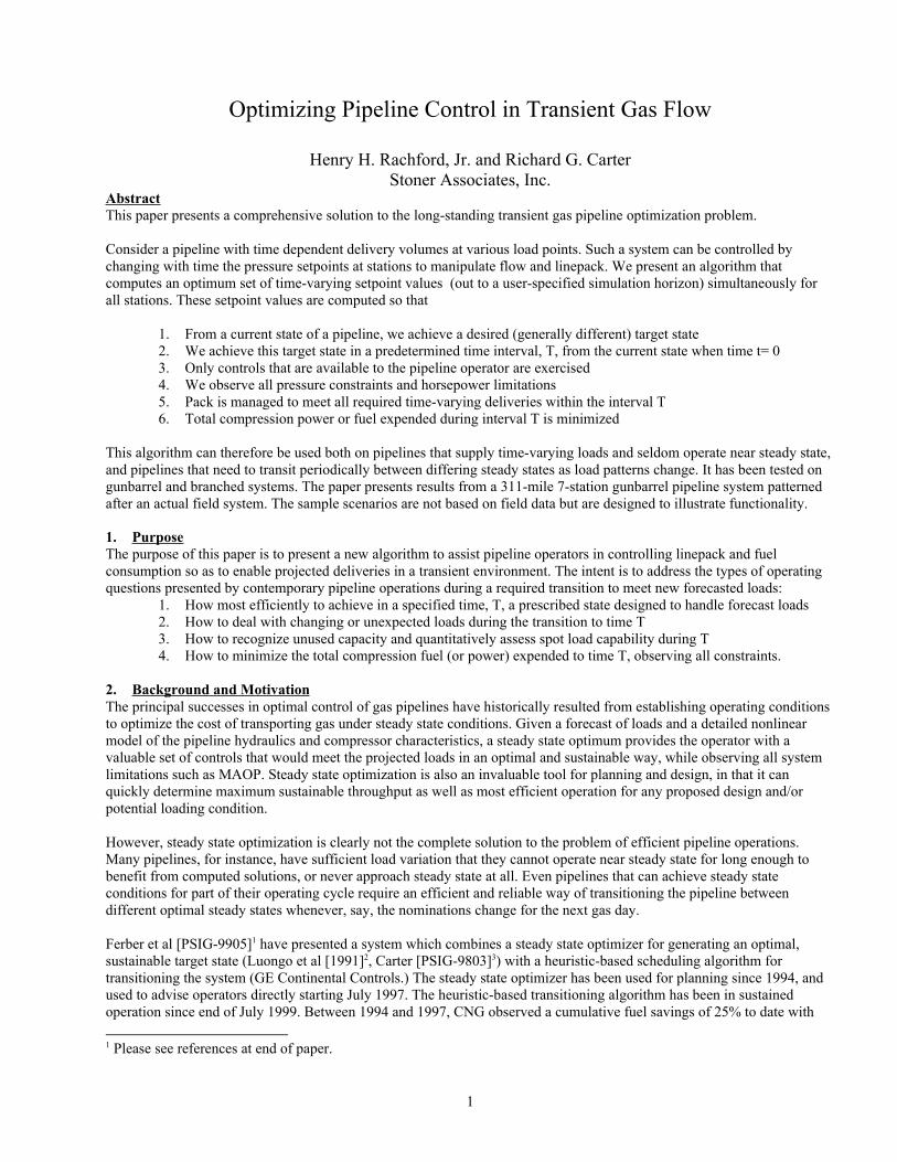
The results of the Scenario 1 simulation using the manual Control Set shown in Figure 2d are detailed in Figure 3 above. Figure 3a shows the fuel rate of usage by station for 16 hours operation. Here the fuel is related to theoretical compression power by Equations 1 and 2 with Cm taken as 0.6 and τm taken as 0.4. A plot of this function is given in Appendix A.

Recall the intent in the optimized Scenario 2 below is to achieve the target steady state in T=8 hours. As noted above the manual control set proposed here does not provide control of the time interval to achieve steady state: you take what you get. We observe that with this strategy the flow does not quite settle to the desired steady state in twice the desired time. As you can see in Figure 3 several other of the hydraulic consequences of the manual Control Set are noteworthy. This control quickly moves the discharge pressure set points to their target values. But the pressures do not track the setpoints. This results because there is inadequate power available at the stations.

For Scenario 2 the maximum available theoretical power at Stations 1 through 7 is, respectively, 12,500, 12,500, 7,500, 12,000, 8500, 8000, and 4500 HP. We note that the Scenario 1 strategy quickly causes each of the compressors to be constrained by the available power so that the discharge pressures at the stations do not track the set points. This is illustrated in Figure 3d. Please compare this Figure with Figure 2d. Indeed, with this control not all the set points were achieved until almost 8 hours into the transition. For completeness, recall the pressure constraints for all scenarios are: a maximum discharge pressure of 1000 psi, and a minimum pressure of 500 psi at all station suction/delivery points.

Another aspect of the simulation is the total fuel usage during the transition. It is computed using Equations 1 and 2. The aggregate fuel used during the time interval plotted is shown in Figure 3c. On the axis at the left in blue is the instantaneous fuel usage with time at all stations. On the axis at the right in red is the integral in time of the blue curve. Thus, the value at 16 hours of the red curve represents the total fuel usage in MMCF expended using Scenario 1 control strategy. That the cumulative fuel usage line (red) is almost straight emphasizes the fact that the fuel usage rate throughout the 16-hour interval remained at or very near the maximum usage possible.

Scenario 1 management of line pack during the 16 hours is shown in Figure 3b. The left axis shows the pack in MMCF (Millions of Standard Cubic Feet) by pipe, and the right axis shows the total pack in all the pipes of the 311-mile system. For comparisons to follow note the pack management with this control strategy ramps the total pack larger than will be needed in the final state. It is mostly the dissipation of this excess pack that seems to cause the transients in the system for the last 8 hours of the scenario.

Scenario 2 Optimized Control Set

For Scenario 2 we use the Control Set determined by the optimization algorithm with T=8 hours. This algorithm has as its goals: 1) Matching the target state at T, 2) Avoiding all constraints (minimum suction pressure, maximum discharge pressure, and maximum available power) and 3) Minimizing the total fuel consumed (Using Equations 1 and 2 to relate fuel rate to theoretical power). Deliveries are those of Figure 2c.

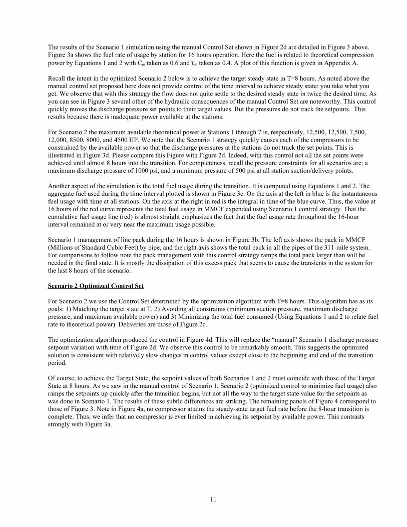
The optimization algorithm produced the control in Figure 4d. This will replace the “manual” Scenario 1 discharge pressure setpoint variation with time of Figure 2d. We observe this control to be remarkably smooth. This suggests the optimized solution is consistent with relatively slow changes in control values except close to the beginning and end of the transition period.

Of course, to achieve the Target State, the setpoint values of both Scenarios 1 and 2 must coincide with those of the Target State at 8 hours. As we saw in the manual control of Scenario 1, Scenario 2 (optimized control to minimize fuel usage) also ramps the setpoints up quickly after the transition begins, but not all the way to the target state value for the setpoints as was done in Scenario 1. The results of these subtle differences are striking. The remaining panels of Figure 4 correspond to those of Figure 3. Note in Figure 4a, no compressor attains the steady-state target fuel rate before the 8-hour transition is complete. Thus, we infer that no compressor is ever limited in achieving its setpoint by available power. This contrasts strongly with Figure 3a.

11

Figure 4. Results from Scenario 2 Control Set (Optimized Fuel Strategy)

4a. FUEL USE RATE BY STATION, SCENARIO 2

0

1

2

3

0 4 8 12 16

HOURS

FUEL

, MM

CFD

"FUEL1" "FUEL2" "FUEL3" "FUEL4" "FUEL5" "FUEL6" "FUEL7"

4b. PACK BY PIPE AND TOTAL PACK, SCENARIO 2

0

20

40

60

80

100

120

0 4 8 12 16

HOURS

PACK

, MMC

F

500

510

520

530

540

550

560

570

580

TOTA

L PA

CK, M

MCF

PACK1PACK2PACK3PACK4PACK5PACK6PACK7TOTPACK

4c. TOTAL AND CUMULTIVE FUEL RATES, SCENARIO 2

8

9

10

11

12

13

14

15

0 4 8 12 16

HOURS

0

2

4

6

8

10

12

TOTFUELCUMFUEL

4d. STATION DISCHARGE PRESSURES, SCENARIO 2

600

650

700

750

800

850

900

950

0 4 8 12 16

HOURS

STA1STA2STA3STA4STA5STA6STA7

Note also, the pack management in the upper right panel of Figure 4b is quite different from that in Figure 3b. After the first hour the total pack rather smoothly ramps to its final value over the next six hours, then smoothly curves into its asymptotic steady-state value without overshooting the final value at all. In fact, the only overshoot in the pack of consequence in any pipe is that in Pipe 7. It is seen to overpack significantly just before the end of the 8-hour transition period. The interpretation of these results will be discussed in more detail later.

Another observation of importance is seen in Figure 4c. Just as in Figure 3c for Scenario 1, this panel shows the total Scenario 2 instantaneous fuel usage for all stations (left axis in blue) as well as the integral of the fuel usage (right axis in red). Note that during the early part of the 8-hour transition, the total fuel rate is remarkably constant at a rate substantially less than the fuel rate at target conditions. This contrasts significantly with the corresponding panel Figure 3c which shows the fuel rate to be comparable to or greater than the target fuel rate for most of the transition time. The foregoing results are emphasized by observing the more marked break in the cumulative fuel line in red in Figure 4c as compared with that in Figure 3c. We note this means the rate of fuel usage is markedly lower below the transition time of 8 hours than at the target steady flow conditions after 8 hours.

The integral of the fuel usage over the 8-hour transition period for Scenario 2 is about 17% less than the fuel usage of Scenario 1, and indeed this excess fuel usage has not achieved the desired result. This, of course, is one of the benefits of optimization. However, insofar as Scenario 1 has not achieved the Target State at this time whereas Scenario 2 has the comparison at 8 hours is not quite appropriate. As time progresses, Scenario 1 eventually converges to the specified optimal

12

steady Target State, and consequently the Manual Control does eventually (around 16 hours) become close to optimal, but not before using a great deal more fuel during the first 8 hours. Despite this eventual convergence and the averaging effect of long time intervals, by sixteen hours the Optimal Control has still used 5% less fuel cumulatively than the Manual Control while supplying the same delivery schedule.

Another noteworthy observation is that even though there has been a major change in the delivery flow rate within the final hour of the transition, the optimal control successfully achieved the target steady state within quite close tolerances. This is seen by observing the fuel usage rate and the line packs to be essentially flat with time after 8 hours. This means the target steady state was approximated quite closely at that time by the control strategy from the algorithm. The most striking point is that the control shown in Figure 4d was still changing some values significantly during the period from 7 to 8 hours, yet the whole system settled quickly to the target steady state at the end of the 8-hour transition period.

To study the differences further, other comparisons are revealing. Consider that minimization of fuel usage using the Scenario 2 strategy is almost equivalent to the minimization of total theoretical power expended for compression. This follows because for most of the transition period the fuel rate is almost constant for each compressor except the small compressor at Station 7. This means that the fuel efficiencies as implied by Equations 1 and 2 are almost constant. Thus, for 6 of the compressors, the theoretical power is approximately a constant multiple of the fuel.

Figure 5. Comparison of Theoretical Power Usage between Scenarios 1 and 2.

5a. HORSEPOWER BY STATION, SCENARIO 1

0

2000

4000

6000

8000

10000

12000

14000

0 4 8 12 16

HOURS

HP1HP2HP3HP4HP5HP6HP7

5b. TOTAL AND CUMULATIVE POWER, SCENARIO 1

0

10000

20000

30000

40000

50000

60000

70000

0 4 8 12 16

HOURS

0

0.2

0.4

0.6

0.8

1

TOTPW

INTGRALPOW

5c. HORS EPOWER BY S TATION, SCENARIO 2

0

2000

4000

6000

8000

10000

12000

14000

0 4 8 12 16

HOURS

HP1

HP2

HP3

HP4

HP5

HP6

HP7

5d. TOTAL AND CUMULATIVE POWER, SCENARIO 2

0

10000

20000

30000

40000

50000

60000

70000

0 4 8 12 16

HOURS

0

0.2

0.4

0.6

0.8

1

TOTPW

INTGRALPOW

13

The results in terms of theoretical power are shown in Figure 5 above. The Figure 5a shows the theoretical power usage with time for each of the compressors using Scenario 1 (manual) control strategy. Figure 5b shows the total theoretical horsepower summed over all stations (in blue on the left axis) and the integral of the power over time T (in red on the right axis expressed as millions of horsepower hours). Figures 5c and 5d show the corresponding plots for the control strategy of Scenario 2 (fuel-use optimized). Observe in Figure 5 the close correspondence in Scenario 2 between the integral of total

horsepower used, the corresponding integral of total fuel usage and the integral of the theoretical power expended as observed in Figure 4.

The reason for introducing plots for the theoretical power is to enhance understanding how the power is used to carry out the required 8-hour task. For this it is helpful to focus attention on the frictional pressure losses. During the simulation sufficient information is captured to allow computing the frictional pressure loss throughout the gunbarrel. The frictional pressure drop for each pipe can be computed as the integral along the length of the pipe of the friction factor times the density times the square of the velocity divided by pipe diameter converted to pressure units. Integrating the product of the frictional pressure drop calculated above times the area times the local velocity in the pipe and adjusting units yields the rate of power loss due to friction along each pipe expressed as horsepower. Summing this power for all pipes yields the total instantaneous power loss due to friction. Integrating the latter with time yields the horsepower hours lost due to friction during the task. This puts this value on a basis comparable to the total theoretical horsepower expended by the stations. And it reveals how the power input is divided between losses due to friction and the potential energy delivered with the gas as pressure.

Figure 6. Comparing Frictional Losses and Station Pressure Differentials

6a. FRICTIONAL POWER LOSS, SCENARIO 1

0

20000

40000

60000

0 4 8 12 16

HOURS

0

0.2

0.4

0.6

0.8

"TOTFPL""INTGFPL"

6b. STATION PRESSURE DIFFERENTIALS, SCENARIO 1

-250

-125

0

125

250

0 4 8 12 16

HOURS

PD1

PD2

PD3

PD4

PD5

PD6

PD7

ZERO

14

6c. FRICTIONAL POWER LOSS, SCENARIO 2

0

20000

40000

60000

0 4 8 12 16

HOURS

0

0.2

0.4

0.6

0.8

"TOTFPL"

"INTGFPL"

6d. STATION PRESSURE DIFFERENTIALS, SCENARIO 2

-250

-125

0

125

250

0 4 8 12 16

HOURS

PD1

PD2

PD3

PD4

PD5

PD6

PD7

ZERO

This follows because the only ways in which theoretical power can be dissipated in the scenarios studied here (in which the flow is assumed to be isothermal through horizontal pipes) is 1) Dissipated through friction, 2) Stored as potential energy in line pack and 3) Delivered as potential energy in the delivered gas. Insofar as the required task begins and ends at prescribed states, and even Scenario 1 eventually ends in the required end state, the power budget must be made up of frictionally dissipated power and power delivered as potential energy in the delivered gas. In this particular example the end delivery pressure and rates are fixed functions of time, so that the only differences in potential energy in the delivered gas isthe suction pressures at the stations where deliveries are made. Thus, overpressuring the system at these points would add to power costs entering the optimization.

Figures 6a and 6c, above, show plots of the aforementioned frictional results for both Scenarios 1 and 2, respectively. The manual Control Set of Scenario 1 immediately produces a frictional power loss slightly in excess of the target state rate. This persists during the high packing rate shown in Figure 3b. It then tapers off, and does not rise again until close to 16 hours when the target steady state is finally approximated. By contrast, the optimized Scenario 2 early on produces somewhat less frictional power loss which quickly drops back to a nearly constant 75% of the target steady frictional horsepower cost, maintaining this lower value until close to the end of the transition. Toward the end of the transition, it rises quickly to the target value and, of course, must remain there. Of importance is the total integral of the frictional power loss at the end of 16 hours, insofar as at that time both scenarios have attained the target steady state. At this time, the integral of the frictional power loss in Scenario 1 is about 4% larger than that in Scenario 2. It is revealing to observe that the theoretical power expenditure by all stations was about 10% higher at the same 16 hours in Scenario 1 than in Scenario 2. But if we compare the frictional loss at the end of the transition time, 8 hours, we see that the frictional pressure horsepower loss in Scenario 1 is about 14% larger than in Scenario 2. From these observations collectively we conclude that the excess power goes to increase pack in Scenario 1 (Please recall Figure 3b) which is recovered to supply the frictional losses during the period between 8 and 16 hours. Another comparison is shown in Figure 6b and 6d. This is the pressure differential across stations, that is the difference between the discharge pressure and the suction pressure. The differentials generated by stations 1, 2 and 4 in Scenario 1 are initially higher than for Scenario 2, but the differentials across most of the other stations do not appear to be significantly different.

However, in the case of Station 7, the difference is striking. From the start until near the end of the 8-hour period the pressure differential at Station 7 in Scenario 2 is negative. This means that Station 7 throttles to maintain the discharge pressure, building pack in Pipe 7, as noted earlier. The throttling persists until shortly before the end of the transition when a release of the Pipe 7 pack occurs in a precisely controlled way. Such management of line pack might be considered to be highly counter-intuitive in view of the fact that there will be frictional losses associated with the throttling. However, in retrospect, building energy in Pipe 7 and releasing it in a controlled way to damp transients during the last hour of the transition period seems quite appropriate.

15

Scenario 3, A Shorter Transition Time

Recall the Manual Control yielded the target state in a 16-hour time interval which depended solely upon the hydraulic characteristics of the system. Scenario 2 achieved the target state on demand in an 8-hour transition period. The next scenario will examine the consequences of requiring the target state to be achieved in 6 hours instead of 8.

The comparison between Scenarios 1 and 2 shows the algorithm accomplishes some of its goals: achieving the required state in the required length of time and significantly lessening fuel and theoretical power usage. Scenario 2 showed that in moving from a low rate situation to a high rate in a period of 8 hours, the transition could be made without using more power at any station than was required at that station for the steady target state.

One of the purposes of studying the algorithm described in Section 4 is to examine its potential value as an aid in operations. So let us consider an operational question. Suppose the power limits of Scenarios 1 and 2 were based upon an operational decision to use only a certain set of available compressors which could just supply the power levels required in the target state.. Instead, now assume the operator actually has available more power than was considered for Scenario 2, but wants to achieve the Target State in a shorter time, say in 6 hours instead of 8. Four operational questions of importance in answering the question arise:

1. Can the Target State be achieved in 6 hours? 2. If so, what maximum of power is required by station and when is it applied? 3. What is the total amount of power (or fuel) that will be required? And finally, 4. How should the discharge pressures be adjusted to accomplish these goals?

To answer the question the algorithm was used to find a Control Set without imposing limits on the power usage by any station. However, a goal of minimizing total horsepower-hour usage during the transition replaced the fuel minimization goal. The required minimum and maximum pressure constraints were also continued. It was necessary to modify the supply/delivery rates shown in Figure 2c. This follows because changes in the Delivery at Station 6 and at the End Delivery station were still being made between 6 and 8 hours as seen in Figure 2c. These were moved earlier so as to occur before the 6th hour. Specifically, the End Delivery was ramped from 480 to 780 MMCFD between 5 and 5.5 hours, and then on to agree with the target rate between 5.5 hours and 6 hours. Delivery 6 was also ramped from 270 to 120 MMCFD between 5 and 5.5 hours. The scenario and results are summarized in Figures 7 and 8 below. The delivery schedule described above is shown graphically in Figure 8c, the second figure below. Note that in Figure 8 the time scale plotted is different from that of Figure 7 to allow for more detail in the graphs by removing some of the steady-state part of the results.

Figure 7. A Shorter Transition time. Scenario 3

7a. STATION POWER USAGE, SCENARIO 3

0

2000

4000

6000

8000

10000

12000

14000

16000

18000

0 2 4 6 8 10 12

HOURS, TRANSITION IS 6 HOURS

HP1HP2HP3HP4HP5HP6HP7

7b. PACK BY PIPE, TOTAL PACK

40

50

60

70

80

90

100

0 2 4 6 8 10 12

HOURS, TRANSITION IS 6 HOURS

500

520

540

560

580

PACK1

PACK2

PACK3

PACK4

PACK5

PACK6

PACK7

TOTPACK

TOTAL

16

7c. TOTAL AND CUMULATIVE POWER USAGE, SCENARIO 3

0

20000

40000

60000

80000

-3 2 7 12

HOURS , TRANS ITION IS 6 HOURS .

0

200000

400000

600000

800000

1000000

TOTHP

CUM.HP

7d. DISCHARGE PRESSURE SETPOINTS, SCENARIO 3

650

700

750

800

850

900

950

0 2 4 6 8 10 12

HOURS , TRANS ITION IS 6 HOURS

STA1

STA2

STA3

STA4

STA5

STA6

STA7

The Scenario 3 Control Set is shown in Figure 7d. We see it is qualitatively similar to that of Scenario 2. The resulting power usage is shown in Figure 7a. While similar to the usage shown for Scenario 2, we see here that the power used at each station at some time substantially exceeds its power in the target steady state. There is also substantially more variation with time of the power usage at Stations 4, 5, 6 and 7 than occurred in the longer transition period. (Please compare with Figure 5c.) It is helpful in studying power usage again to plot the instantaneous horsepower usage and the integral of the usage. This is shown for Scenario 3 for a 12-hour period (again twice the transition time) in Figure 7c. Observe that while the total power usage is initially lower than the usage rate in the target steady state, the usage rises steeply after about 4 hours, and oscillates until shortly before the end of the 6-hour period.

Again for insight, please observe the Scenario 3 linepack management in Figure 7b. Much like its counterpart in Figure 4b for Scenario 2 the pack very smoothly rises to its target steady state value without any overshoot. Comparing the linepack management between Scenarios 2 and 3 shows why Scenario 3 requires more power. In both cases the pack increases from 508 to 572, or 64 MMCF. In Scenario 2 this is distributed over 8 hours, for an average rate of 64 X 24 / 8 = 192 MMCFD added to the underlying deliveries. In Scenario 3 the extra pack is distributed over 6 hours which corresponds to 64 X 24 / 6 = 256 MMCFD, a substantial friction increase in the load.

Figure 8. Further Detail for Scenario 3 Operation

8a. FRICTIONAL POWER LOSS, SCENARIO 3

0

10000

20000

30000

40000

50000

60000

70000

0 2 4 6 8

HOURS , TRANS ITION TIME IS 6 HOURS

0

0.1

0.2

0.3

0.4

0.5

0.6

TOTFPL

INTGFPL

CUMULATIVE FRICTION LOS S

8b. SUCTION PRESSURES BY STATION, SCENARIO 3

550

600

650

700

750

800

850

0 1 2 3 4 5 6 7 8

HOURS, TRANSITION IS 6 HOURS

STA1

STA2

STA3

STA4

STA5

STA6

STA7

17

8c. SIDE, END DELIVERIES, SCENARIO 3

-400

-200

0

200

400

0 2 4 6 8

HOURS, TRANS ITION TIME IS 6 HOURS

0

100

200

300

400

500

600

700

800

900

DLY_1DLY_6ENDLY

S upply 1

Delivery 6

End Delivery

8d. STATION DELIVERY RATES , SCENARIO 3

0

200

400

600

800

1000

1200

1400

0 2 4 6 8

HOURS . TRANS ITION IS 6 HOURS

STA1

STA2

STA3

STA4

STA5

STA6

STA7

Again Pipe 7 pack is managed so as to achieve the necessary damping of transients in approaching the target. But in contrast to Scenario 2, in which only pipe 7 pack exceeded the target pack, in Scenario 3 pipes 4 and 5 also overpacked during the period T. Please observe, however, that even though pipes 4, 5, and 7 overpacked during Scenario 3, the total pack did not.

To complete the study of the 6-hour transition it is helpful again to examine the role of friction in the power budget expended in the transition. For this please see Figure 8a. Comparing this with the total theoretical power as shown inFigure 7c shows that frictional loss tracks the total power input quite closely. Again, in the interest of plotting detail, recall the time scale plotted in Figure 8 spans only 8 hours instead of the 12-hour span of Figure 7, but of course the transition time is 6 hours for this scenario. At the target state, friction accounts for about 85% of the power input. It is surprising that in this scenario, which minimizes theoretical power usage, it also roughly approximates that same ratio throughout the transition period. It is meaningful on this point to observe the discharge flow rates from all the compressor stations in Figure 8d. Because the initial and target states are so different, clearly the flow rates must change. But the striking observation of this figure is that apart from an initial surge, the flows through each of compressors 1, 2, and 3 (where heavy power inputs occur) maintain rates that are reasonably constant during the first 4 of the six-hour transition.

The foregoing observation is in retrospect quite plausible. Friction uses the dominant part of the power budget, and for a given throughput the frictional losses will be minimized if the flow is maintained at a constant rate rather than undergoing substantial changes. The latter statement follows because from elementary principles the frictional power loss over T is proportional to the integral over T of the cube of the flow divided by the square of the average density. There is of course the side relation that the integral of the flow over T be the required delivery. So to minimize the integral of the cube of flow subject to holding the integral of flow constant, we should maintain as nearly constant flow as possible. As remarked above, this is close to what we observe in the figure. It is interesting that the control found by the algorithm in this case produces flows consistent with the foregoing simple analysis of the frictional budget.

Also, please examine the suction pressures by station in Figure 8b. First, this shows that Scenario 3 does not violate the minimum pressure constraint at any station. Another point of this figure is to observe the use of pressure control at Station 7. Comparison of the suction and discharge pressures (Figure 7d) at Station 7 shows that for a time between 4 and 5 hours, Station 7 functions as a pressure reducing station rather than a compressor station, throttling gas to manage Pipe 7 line pack. This is reminiscent of the strategy of Scenario 2. Again, the pressure is built up in Pipe 7 in the period before the end of the transition for use in damping the transients through a precisely controlled release just before 6 hours.

Operationally, Scenario 3 demonstrates a capability of answering the practical questions raised earlier which impact the operability of the pipeline. The practical answers that could not in general be answered in advance otherwise are: 1) The Target State can in fact be achieved in 6 hours. 2) It cannot be achieved without increasing the horsepower above that required in the Target State, and it can be achieved if theoretical power is available at the seven stations, respectively, as

18

follows: 18000, 18500, 11500, 14500, 11500, 14500, and 9000 HP. 3) The theoretical power required is shown in Figure 7, and 4) The control pressures should be adjusted with time as shown also in Figure 7d to achieve the target. Providing such information in advance will enable the pipeline operator to make better-informed choices. Namely, does he want to do this?

Scenario 4, Can we Do the Deal?

Another operational problem the transient optimization algorithm might profitably address is examined with Scenario 4. Again, we use the same initial and target states shown in Figure 2. In this scenario, however, we assume the forecast is to increase the low initial flow over a 24-hour period (T=24), the high delivery rate coming late in the period. Scenario 4 will address the operational question of side stream transportation of gas during the transition period. This is akin to a frequently arising gas control problem concerning whether there is spare carrying capacity during a day.

In this scenario assume the forecast requires the high delivery associated with the Target State to begin only 3 hours before the end of the 24-hour transition period. Before that time it follows the curve up to time 7 hours shown on Figure 2c. Specifically, the schedule for the end delivery begins at 280 MMCFD, rises to 480 MMCFD between 0.75 hours and 1.5 hours, remaining at 480 MMCFD until 21 hours at which time it ramps from 480 to 827 MMCFD in a quarter-hour. The delivery at Station 6 will continue to follow the same pattern shown in Figure 2c. This delivery schedule leaves a lengthy period in which the system is only lightly loaded. Suppose there is a potential client offering to purchase gas transport today of 200 MMCF between Station 2 and Station 7. But the gas is to be delivered at station 7 before it is available as a supply at the suction of Station 2. It must be delivered at 400 MMCFD at station 7 for 12 hours beginning 4 hours into the transition. Gas can be supplied at Station 2 suction at 400 MMCFD at a pressure of 850 psig, but the supply at Station 2 cannot begin until 9 hours into the 24-hour transition period. This means that for five hours the client is borrowing from our line pack. (Receipts and deliveries are summarized in Figure 9c.)

The questions from the marketing office are “Can we make the deal, and if so, what will it cost?” Assuming all flows occur as proposed and the final Target State of the pipeline is not to be compromised, how should the questions be answered?

The first question of importance is whether the line and compression capacity exists to permit the transport under these conditions. The second would be how much power is required, and when. A third is whether the suction pressure at Station 2, where delivery of the 400 MMCF gas must be accepted, can be kept below 850 psig. The algorithm is again used. The side flow conditions are entered, and constraints are placed only on the minimum and maximum pressures, allowing the power utilization to be unconstrained, but again penalizing the total power usage.

As mentioned above Figure 9c shows the delivery schedule corresponding to the scenario. Recall delivery is plotted as a positive value, receipts are plotted with negative values. Again note that there is a supply (negative graph) at Station 1. This supply begins at 262 and ramps to 367 MMCFD between zero and 0.75 hours. It retains this value for the remainder of the scenario. The end delivery begins at 257 and ramps to 480 MMCFD at the end of 1.5 hours. It remains at this level until 19 hours at which time it increases to the target state value, 827 MMCFD. Note that at Station 6, as in scenario 3 there is an increase in the original delivery rate from 120 to 270 at 1.5 hours. At 5 hours this rate is reduced back to the target state value, 120.

Figure 9. Can We Make the Deal? What does it cost? Scenario 4.

19

9a. HORSEPOWER BY STATION, SCENARIO 4

0

4000

8000

12000

16000

0 12 24 36

HOURS. TRANSITION TIME IS 24 HOURS

S TA1S TA2S TA3S TA4S TA5S TA6S TA7

9b. STA. DISCHARGE PRESSURE SETPOINTS, SCENARIO 4

600

700

800

900

1000

0 12 24 36

HOURS . TRANS ITION IS 24 HOURS

STA1

STA2

STA3

STA4

STA5

STA6

STA7

9c. SIDE, END DELIVERIES, SCENARIO 4

-500

-400

-300

-200

-100

0

100

200

300

400

500

0 12 24 36

HOURS. TRANSITION IS 24 HOURS

0

100

200

300

400

500

600

700

800

900

DLY_1DLY_6DLY_7DLY_2ENDLY

SUPPLY 1

SUPPLY2

DELIVERY 7

DELIVERY 6

END DELIVERY

9d. STATION SUCTION PRESSURES. SCENARIO 4

600

650

700

750

800

850

900

950

0 5 10 15 20 25 30 35 40

HOURS . TRANS ITION IS 24 HOURS

STA1

STA2

STA3

STA4

STA5

STA6

STA7

The principal operational questions to be answered in this scenario are introduced by the side flows at Station 7 where a delivery at 400 MMCFD begins at 4 hours and persists to 16 hours for a total delivery of 200 MMCF. This gas is delivered from line inventory until the supply flow at Station 2 begins at the rate of 400 MMCFD at 9 hours. This supply persists until 21 hours at that rate, replacing the 200 MMCF. But 83 MMCF is borrowed from inventory insofar as receipt does not begin until 5 hours after the delivery begins. The most important question is feasibility. We must find if the system can hydraulically handle the delivery and receipt without violating minimum or maximum pressure constraints within the level of available power. The answer will again be determined by freeing all constraints on station power in applying the algorithm while continuing to penalize the total power utilization and apply pressure constraints. This is similar to the solution in Scenario 3. Figure 9 above shows the results of applying the algorithm with these goals.

The recommended control found by the algorithm for the 24-hour transition period is shown Figure 9b. The time values at which the control set is determined were spaced at 15-minute intervals, i.e., every 15 minutes a new discharge pressure was determined for each of the 7 stations. This means the control set consists of 7 X 24 X 60 / 15 or 672 variables. Again, the setpoints for the compressor stations were ramped linearly in time between control set values. Observe that because there are so many disturbances imposed on the system by the changing loads, the controls do not appear to be as smooth as they appeared in the earlier scenarios. Part of this is because the time scale is several times longer. Further the reaction of the pipeline system is related to its hydraulic time constants, and not to the transition period we choose. Thus, when we plot on the basis of the longer transition period the controls appear to move much faster.

20

Figure 9a shows the resulting power required as a function of time. The effects of the disturbances introduced by the changing loads and receipts show very clearly in the power-versus-time plots. For example, one can correlate power usage shown in the upper panel with the changes in the receipt/delivery plots in the panel immediately below. In particular, the total need for compression begins early, earlier in fact than the onset of the 400 MMCFD delivery at Station 7. This means the algorithm correctly prepared for a future situation. It produced a control to pack the system in advance to prepare for this delivery from linepack.

The need for compression drops quickly, especially at Station 1 immediately after the receipt of gas at Station 2 begins. Then as the delivery of the 400 MMCFD at Station 7 terminates, there is a marked diminution of power requirements until shortly before the end of the transition period. Note that the power usage for all compressors flattens out and each attains its steady target state value quickly at 24 hours. This proves the algorithm successfully made all deliveries as well as meeting the Target State.

Figure 9d, which shows suction pressures versus time, is important also for examining feasibility. Recall the gas received at Station 2 cannot be supplied to the system at pressures in excess of 850 psig. The delivery into the system begins at 9 hours and lasts through 21 hours. The suction pressure at Station 2, plotted in magenta, shows the pressure there peaks at less than 800 psig between 18 and 21 hours. Receipt of the replacement gas is thus seen to be feasible on the projected schedule.

Application of the algorithm has provided the physical answer to the question “Can we make the deal?” The method shows that it is possible hydraulically and, moreover, shows the level of power and fuel costs and the pattern of compressor usage required to make the proposed deliveries. The question then becomes “Should we make the deal?”, for it is now one of economics, not of playing the odds with the hydraulics.

6. Discussion of Possibilities

For brevity, these simple examples show just a few of the ways transient optimization might be used in contemporary pipeline operations as well as for “what if” studies. Many other variations are possible. Let us consider some other ways the method can be used, along with algorithmic extensions that we have already examined, and our expectations for the future.

Although the examples in this paper are gunbarrel pipelines, we have also optimized branched network operation by this approach. The character of observed solutions was very similar. Looped systems are expected to be a straightforward extension. Similarly, it is not a requirement that all time-dependent deliveries and receipts occur at station inlets, nor that stations be controlled by discharge pressure. These choices were purely arbitrary in generating the examples in this paper. Output of the transient optimization algorithm is consistent with station control by suction pressure, discharge pressure, or horsepower, as needed for optimum interfacing in individual Scada environments.

Setpoints were updated at 15-minute intervals in our examples, but less or more frequent updates are also perfectly permissible. The solution quality will decrease somewhat with less frequent updating, but the burden on operators will also decrease if the SCADA interface is not automated. To address this point with a quantitative example, please see a repeat of Scenario 2 as Scenario 2A in Appendix B. This shows the results of updating the setpoint values every hour during the 8-hour transition instead of the 15-minute intervals used in Scenario 2.

For our tests, we used either fuel or power as objectives to be minimized. These choices are traditional, but there is nothing special about them. Many other objective functions could be included just as easily. For instance, there is a growing trend to use electric power for compression. The unit cost of electricity frequently depends upon the time of day of power usage or on the previous average power usage. The electric power cost-dependence upon such variables can be written into the objective; this would then change the optimization goal from one of minimizing gas fuel usage to one of minimizing electric costs. This can be done locally by station in the event some stations are gas fired while others use electric power. Of course, the constraints on pressure and maximum power usage will continue to apply as appropriate.

Another significant cost of operation of pipelines is the regulatory penalty in some areas due to emission of flue gases, either greenhouse gases or more especially flue gases with concentrations of NOx, or oxides of nitrogen. The latter contribute in part to smog and acid rain. If emissions models are available for compressor usage (they are increasingly being supplied along with the machines themselves by manufacturers, especially in 2-cycle reciprocating engines) these can

21

be incorporated into the cost objective. Then the algorithm would minimize not only the cost of fuel, but at the same time the cost of penalties due to emission of exhaust gases.

Another extension that appears attractive is the planning of curtailment that might become necessary due to loss of equipment or supply, or some other contingency. During the delivery day for a pipeline, some event often leads to an upset of the planned operation. A supply might be lost. A compressor station may lose capacity through equipment failure. A sudden large load may appear, an increasingly frequent occurrence as the incidence of gas-fired electric generation plants proliferates. If the scheduled deliveries become infeasible with available resources as a result of such an event, the operator may be forced to curtail delivery to an interruptible client. The most important operational questions arising in this case take several forms: 1) Is any curtailment necessary? 2) If so, when should the curtailment take place? And the related question 3) Where should the curtailment take place, and how severe must it be?

The costs of curtailing interruptible delivery can readily be added in the cost objective in the algorithm. In addition to minimizing other costs as described earlier, the algorithm would then minimize the cost of curtailment while maintaining feasibility of delivery to the non-curtailed clients. This would allow an immediate response to foregoing questions which always must be answered, and usually without delay in the event of unexpected contingencies. This follows because the solution of the resulting scenario would then automatically point to the time and locations at which curtailment will incur at least cost, and provide the necessary control for achieving the minimum cost schedule.

Applications involving the use storage fields would also be a logical extension, which should in principle be straightforward. This follows because the cost of compressing gas to storage is well quantifiable in terms of the variables simulated during the transition time for any scenario. The principal costs to be quantified involve the line pressure at the suction of the injection compression station, the field back-pressure and the rate of injection. Thus, the average cost of gas compressed into the storage field can be quantified during any period where excess line capacity is available. This would lead to minimizing the cost of the stored gas. Given an average cost of stored gas, a similar set of questions could be answered in managing the use of stored gas to handle contingencies.

However, we hasten to point out that our numerical experience with the aforementioned extensions is yet slim. But we mention them because the potential value of success in such applications would appear attractive. For ideal usage, a transient optimizer would be part of a bigger picture. Current pipeline conditions are always needed as a starting point. Thus, these would need to be determined using SCADA data and pipeline state estimation software. Future loads need to be predicted using nominations, or forecasting software. The Target State needs to be computed using steady state optimization, which also needs future load estimates. These processes would all tie together to feed the transient optimizer. The results could then be passed into an advisory report environment for operators, planners, and marketers, or they could be passed on to other simulation packages for verification and display, as we have done in our examples.

What if predicted loads fluctuate due to changes in weather forecasts or market conditions? In such an event the transient optimization can quickly be rerun under the updated conditions to revise its previously computed control. Computing a revised solution will be substantially faster than the original computation because of the iterative nature of our solution process and the reuse of previous information. This will provide a significant logistical advantage for analyzing large systems.

Figure 10 below illustrates how the information flow amongst the programs would occur to provide the structure discussed above.

Figure 10. A Role for Transient Optimization

22

Using Transient OptimizationThe Role it Can PlayPipeline

Scada

State Finder

Load ForecastWeather, History

Steady StateOptimizer

TransientOptimizer

Changes:Now untilTime T

Target state

Predictor Display

Control

PreviewHours T

Opportunity Scenariop

Of perhaps most importance in the foregoing flow chart is the communication above called the “Opportunity Scenario.” This is similar to Scenario 4 in that it enables answering the question “Can we make the deal?” There will almost always be unused capacity in the pipeline. It might not be evident from a simple steady-state analysis, but there may be times during the day in which an opportunity can be seized if the timing is right and the tools available to detect it.

7. Conclusions

This paper has described a comprehensive transient optimization and pack management algorithm for the operation of a gas transmission pipeline. The algorithm is immune to the inventory depletion problem, and is fast enough to be practical on existing computers. It uses a rigorous transient model of the nonlinear pipeline hydraulics rather than any simplification. Tests on straight and branched systems have generated robust, non-intuitive solutions for achieving stressful fluctuating delivery schedules. And these are accomplished at substantial energy and fuel savings when compared with typical field controls.

In our examples optimization resulted not only in achieving the target state at the required transition time, T, but in doing so saved 17% of the fuel used during T by a typical manual control strategy which took over twice as long to achieve the target state.

Appendix A

In Section 4, the relation between fuel usage and theoretical power was discussed. The relation coded for the implementation of the algorithm was given as Equations 1 and 2. Two parameters appeared in these relations, a value of Cm

and τm. In the minimization of fuel usage in Scenario 2 these parameters were taken as 0.6 and 0.4, respectively. To aid in interpreting results, Figure 10 shows a plot of F/(Hm•NFR) versus H/ Hm. In the figure F is the fuel rate in SCFD, H is the theoretical power used, Hm is the maximum available theoretical power, and NFR is the nominal fuel rate in SCFD/HORSEPOWER.

23

Figure 10 Fraction Fuel VS Fraction Power

0

0.1

0.2

0.3

0.4

0.5

0.6

0.7

0.8

0.9

1

0 0.1 0.2 0.3 0.4 0.5 0.6 0.7 0.8 0.9 1

H/Hm

F/(H

m X

NFR

)

Series1

24

Appendix B

In the discussion above, the point was made that there is substantial flexibility in the choice of the time intervals during the transition time T on which the control values are determined. In Scenario 2, the control values for each station were determined on 15-minute intervals, as they were in all other of the Scenarios based upon optimization. The question naturally arises, “Do the results depend strongly upon this choice?” One reason for the question is that the burden of control with SCADA systems that are not automated might be considered excessive if the pressure control must be changed at each station every 15 minutes.

In Scenario 2A, presented here, the control was determined on 1-hour intervals. This means that 4 times fewer values were determined by the optimization, and only a fourth as many adjustments in target setpoints for the stations need be made. How much influence does this coarser granulation have on results? Figure B1 shows the same results for Scenario 2A as those shown in Figure 4.

Figure B1. Scenario 2A. Optimization Results using 1-Hour Control Intervals

B1a. FUEL USAGE RATE, SCENARIO 2A

0

1

2

3

0 4 8 12 16

HOURS , TRANS ITION IS 8 HOURS

FUEL1FUEL2FUEL3FUEL4FUEL5FUEL6FUEL7

B1b. PACK BY PIPE, TOTAL LINEPACK, SCENARIO 2A

40

50

60

70

80

90

100

110

0 4 8 12 16

HOURS. TRANSITION IS 8 HOURS

500

520

540

560

580

PACK1

PACK2

PACK3

PACK4

PACK5

PACK6

PACK7

TOTPACK

B1c. TOTAL FUEL RATE, CUMULATIVE FUEL, SCENARIO 2A

8

9

10

11

12

13

14

15

0 4 8 12 16

HOURS , TRANS ITION IS 8 HOURS

0

1

2

3

4

5

6

7

8

9

TOTFUEL

CUMFUEL

B1d. STATION DISCHARGE PRESSURE SETPOINTS, SCENARIO 2A

600

650

700

750

800

850

900

950

0 4 8 12 16

HOURS . TRANS ITION IS 8 HOURS

STA1STA2STA3STA4STA5STA6STA7

Comparing Figures B1d and 4d shows substantial similarities in control. It is clear that the control of Scenario 2A is a great deal coarser than that of Scenario 2. But this shows up in the quality of the optimized solution only slightly. For example, we see that the fuel rate undergoes somewhat more change following the 8-hour transition than does that of Scenario 2. One of the goals of the optimization is to achieve the target state. Insofar as the target state is steady, attaining it at T=8 hours would result in a constant fuel rate at 8 hours. While neither the fuel rates of Scenario 2 nor Scenario 2A is exactly constant at the end of the transition period, it changes more after 8 hours in Scenario 2A than it does in Scenario 2. Please compare Figures

25

B1a and 4a. This means that the state acquired by the control of Scenario 2 got closer to the target than that of Scenario 2A. Insofar as the states acquired by either Scenario 2 or 2A yield power changes following the 8-hour transition which are of no engineering consequence, other quantitative differences may be of greater operational importance. Comparing Figures B1c and 4c shows the effect on fuel required. The 8-hr fuel usage in Scenario 2 is 3.833 MMCF, while that of Scenario 2A is 3.990 MMCF, or 4% more.

Scenario 2B. For completeness in studying this issue, another scenario (Scenario 2B) was run using the same deliveries and target time as Scenario 2. Scenario 2B was run using 5-minute instead of 15-minute intervals for determining discharge setpoint values. Scenario 2B (which is not shown in this paper) shows the 8-hour fuel usage to be 3.799 MMCF, or approximately 0.9% less than that for Scenario 2. We conclude from this that control on 15-minute intervals uses only slightly more fuel than the best strategy we can likely use. The control of Scenario 2B is not appreciably different from that of Scenario 2. It has only a somewhat sharper rise in the control setpoints at the start, and a bit more fine structure near the end of the transition. It is favorable that the character of the solution is essentially unchanged between the 15-minute case which solves for 224 numbers and the 5-minute case (Scenario 2A) which determines 672 control set variables for the same physical situation.

References:

3Carter, R.; “Pipeline Optimization: Dynamic Programming after 30 Years,” [PSIG-9803]

1Ferber, P., Linden, P., Goodreau, M., Basu, U., and Venkataramanan, G.: “Gas Pipeline Optimization [PSIG-9905]

2Luongo, C. A., Yeung, W. C., and Gilmour, B. J.: “Optimizing the Operation of Gas Transmission Networks,”ASME International Computers in Engineering Conference, Santa Clara, California, August 1991

4Westhoff, M. A.: “Using Operating Data at Natural Gas Pipelines,”International Symposium on Transportation Recorders, Arlington, VA. May 1999

26