1

Optimizing large scale emergency medical system operations on highways

using the hypercube queuing model

Ana Paula Iannoni

Ecole Centrale Paris

Laboratoire Genie Industriel, Chatenay Malabry 92295, France iannoni93@hotmail.com

Reinaldo Morabito

Department of Production Engineering

Federal University of Sao Carlos, SP 13595-905, Brazil morabito@power.ufscar.br

Cem Saydam

Department of Business Information Systems and Operations Management

University of North Carolina at Charlotte, NC 28223, USA saydam@uncc.edu

Please send all correspondence to:

Professor Cem Saydam

Business Information Systems and Operations Management Department

The Belk College of Business

The University of North Carolina at Charlotte

Charlotte, NC 28223

Phone: 704-687-7616

Fax: 704-687-6330

Email: saydam@uncc.edu

Submitted to Socio-Economic Planning Sciences

May 2009

2

Optimizing large scale emergency medical system operations on highways using the

hypercube queuing model

Abstract: In this study we present straightforward optimization methods to address two

problems associated with designing large scale ambulance operations on highways; the question

of location and the issue of districting. Previous approaches tackled small scale problem instances

using exact hypercube queuing models integrated into optimization procedures mainly due to

excessive computer storage and runtime requirements of large problem instances. We overcome

these limitations by embedding a fast and accurate hypercube approximation algorithm adapted

for partial backup dispatch policies in single- and multi-start greedy heuristics. We apply the

proposed methods to a case study for comparisons and present computational results for large

scale problem instances of up to 100 ambulances. The results show that our straightforward

approach is a viable alternative for the analysis and configuration of large scale highway

emergency medical systems, providing reasonable accuracy and affordable running times.

Keywords: emergency medical systems, ambulance deployment, approximate hypercube

queuing model, multi-start greedy heuristic, probabilistic location and districting problems.

1. Introduction

Emergency response systems are in general server-to-customer systems with several

probabilistic aspects, such as the spatial and temporal distributions of emergency calls and server

locations, the availability of servers and the service times. The hypercube model [21, 24], which

is based on spatially distributed queuing theory and Markovian analysis approximations, has been

one of the most effective descriptive approaches used to analyze emergency response systems.

The idea is to expand the state space description of a multi-server queuing system (e.g., M/M/N/

or M/M/N/N system, where N is the number of servers [24]) in order to represent each server

individually and account for the spatial nature of these systems, such as interdistrict dispatching.

Since each server must be in one of two states, either idle or busy, the model requires the solution

of linear systems of O(2N) equations, where the variables are the equilibrium probabilities of the

possible states of the system. With these state probabilities, several important steady-state

3

performance metrics, such as mean user response times, server workloads and fraction of

dispatches of each server to each region, among others, can be estimated.

Examples of applications of the hypercube queuing model in urban emergency medical

systems (EMS) can be found in [6, 9, 10, 13, 21, 24, 25, 28, 32, 34]. Some studies have extended

the original model for application to emergency medical systems (EMS) on highways. For

example, Mendonça and Morabito [27] adapted the model to consider dispatching with partial

backup, Iannoni and Morabito [15] modified that model to consider multiple dispatching of

different types of servers, Atkinson et al. [1, 2] proposed heuristic methods to estimate the loss

probability for large-scale systems, and Budge et al. [8] used approximate hypercube models to

consider station-specific (rather than server-specific) busy fractions and dispatch probabilities,

while allowing for multiple servers at bases.

Although the hypercube queuing model is a descriptive model, it can be combined with

search procedures to optimize spatially distributed and stochastic operating systems. In Larson

(1979), there are several illustrations of research to support location decisions, such as optimal

allocation and dispatching of servers, districting, and short-term repositioning of servers. For

instance, Larson [23] describes how Berman [5] extended the N-median problem (where N is the

number of servers or facilities) using the hypercube model, taking into account server

unavailability and cooperation, in order to minimize the expected average travel time. Other

studies combining exact and approximate hypercube models with optimization procedures to

solve probabilistic location problems have been reported, e.g., in [4, 11, 12, 16-18, 29, 33].

In particular, Iannoni et al. [16] integrated a multiple dispatch partial backup hypercube

model into a genetic algorithm (GA) in order to determine the optimal response areas for the

ambulances (to address a districting problem). Iannoni et al. [17] extended this approach to

optimize two combined decisions: the location of the ambulances and their corresponding

coverage areas (districts), creating what was called a location and districting GA/hypercube

algorithm. Nevertheless, the main drawback of these optimization approaches is the excessive

computer storage and runtime requirements [16, 17]. Even when iterative methods are used to

solve the linear systems involved in the hypercube models, the required computer efforts of the

GA/hypercube algorithms become prohibitive for the analysis of larger systems (e.g., with more

than 30 ambulances) that are found in medium to large cities and highways.

4

Most of the aforementioned studies using exact hypercube models embedded into

optimization schemes focused on small-to-moderate sized applications, thus avoiding major

computational difficulties. In an effort to address larger problems, the present study explores the

benefits of using fast approximate hypercube algorithms embedded into simple greedy heuristics,

which were not explored in [16, 17]. We consider two different problems separately: determining

the location or relocation of ambulances along the highway (a location problem), and the sizes of

primary and secondary response areas (a districting problem). The optimization approaches use

recent hypercube approximations proposed by Atkinson et al. [1], which are based on the single

dispatch partial backup system analyzed in [27]. First, we apply a single-start greedy heuristic

algorithm using these approximations and the original system configuration as an initial solution.

Then, the approach is extended to a multi-start greedy algorithm for which other initial solutions

are randomly generated. It is worth mentioning that other optimization methods that exist in the

literature, such as the ones described in Larson [23], however, given the complexities related to

partial backup, non-homogeneous servers and linear schemes of these systems they cannot be

directly extended to analyze EMS on highways.

In order to directly compare the proposed approach with previous methods, we first

utilized data from a moderate-sized case study of a Brazilian highway. Second, we tested the

algorithms on randomly generated large problem instances with up to 100 ambulances. We intend

to test the strength of these methods by testing very large-scale systems (for example, in Brazil

there are highway EMS systems with relatively large number of ambulances). As we anticipated,

the proposed straightforward approach (using hypercube approximation) requires affordable run

times while providing reasonable accuracy for large problem instances.

This remainder of this paper is organized as follows: section 2 presents a short description

of EMS on Brazilian highways and the partial backup hypercube model used to analyze them.

Section 3 briefly reviews how approximate methods based on this hypercube model can be

derived and applied to the analysis of these systems. Section 4 describes the optimization

algorithms integrated with the approximate hypercube methods to optimize system performance

measures. Section 5 analyzes the outcomes from the application of the proposed methods to the

case study and to other much larger test problems. Finally, section 6 presents concluding remarks

and perspectives for future research.

5

2. The partial backup hypercube model for EMS on highways

The highway EMS considered in this paper was originally studied by Mendonça and

Morabito [27]. This system provides emergency medical treatments on a portion of the main

highway connecting the cities of Rio de Janeiro and Sao Paulo. It has six ambulances located in

six fixed bases along the highway and an operations center located in Rio de Janeiro. When a call

arrives in the operations center, the nearest ambulance is immediately dispatched to the call

location. If the nearest ambulance is busy, then the second nearest ambulance (called backup) is

dispatched. In cases when the two closest ambulances are busy, the call is considered lost to the

system (even if there are other ambulances available) and transferred to another system. This type

of dispatching policy is referred to as partial backup.

Figure 1 illustrates the original configuration of this EMS with its six ambulance bases

along the highway. The distance between two adjacent bases is divided into two districts (called

atoms), each with a specific dispatch preference list. According to this list, and except for

ambulances 1 and 6, each ambulance is dispatched as preferential to two atoms (immediately to

the left and right of its base), and as backup to the two atoms adjacent to the preferential ones

(right and left of the adjacent ambulances on its left and right, respectively). The reader can find

additional details related to this system in [27]. The main assumptions of the partial backup

hypercube model adapted for EMS on highways are:

- The highway is divided into AN geographical atoms (regions), which correspond to

independent sources of calls. Note in Figure 1 that 22 NNA , where N is the number of

ambulance bases. The calls in each atom j arrive according to a Poisson process with arrival rate

j and independently from the other atoms. Each atom has a fixed dispatch preference list

ranking the first and second (backup) ambulances to be dispatched. If both ambulances are busy,

the call is lost, even if there are other ambulances available.

- There are N ambulances spatially distributed along the highway and when idle, they wait for

calls from their bases. An ambulance’s preferential area consists of those atoms to which the

ambulance would be dispatched, if available, even if all other ambulances were also available.

Each ambulance can only be dispatched to its predetermined primary and backup atoms. The

service time of each ambulance includes the set-up time, the travel time and the on-scene time. In

6

general, each ambulance i has a distinct mean service time, i

1 , where i is the service rate. It

is assumed that the travel time between two regions is known or can be estimated by geometric

probability. Variations in the service time that are due to variations in travel time are supposed to

be of second order if compared to variations in set-up and on-scene times.

Figure 1 – Ambulance bases and atoms along the highway

As illustrated in Figure 1, the stretch of the highway under study is divided into NA = 10

atoms. Given that the EMS has N = 6 servers, there are 26 = 64 possible states. Larson [21]

showed that the hypercube queuing system is in a steady state, the flow into each state should be

equal to the flow out of that state. Using the preference list presented in [27], we can generate the

corresponding 64 steady-state equilibrium equations, representing the hypercube model for this

problem. For example, consider the following equilibrium expression for state 110001, where

ambulances 1, 2 and 6 are busy and ambulances 3, 4 and 5 are idle:

)()()()(

)()())((

51100114110101311100110110000

21010001321100001621109876543110001

pppp

ppp

This expression demonstrates a unique aspect of this system; unlike the original

hypercube model in [21], calls can be lost even though there are servers available. As defined in

this expression, the partial backup does not allow the EMS to send an ambulance based in atom 3

to either atom 1 or 2. Substituting any of the 64 equations by the normalizing equation (the sum

of all state probabilities should be equal to 1), we obtain a determined system with 64 linearly

independent equations.

3. The approximate partial backup hypercube model

As mentioned above, as the (exact) hypercube model requires solving a system of 2N

linear equations, the computer runtime requirements can be prohibitive for problems with large N

10 1

5

atom

2 4 6 1 3

2 3 4 5 6 7 9 8

base

7

(servers), especially when the model needs to be solved many times in an optimization procedure.

In order to reduce the runtime required to solve the hypercube model, Atkinson et al. [1]

proposed a heuristic based on this model to analyze systems similar to the case study described in

section 2 (i.e., with the same dispatch policy). This heuristic has a computational complexity that

is linear in N (instead of exponential in N). Further, this approximation is reasonably fast and

accurate in estimating both the loss probability of the system and ambulance specific busy

probabilities (workloads).

As mentioned, EMS on highways operate within a particular dispatching policy, which

considers, for example, partial backup, multiple dispatch, different types of servers and non-

homogeneous servers. Although there are other hypercube approximation methods (not based on

systems of O(2N) linear equations), such as the methods proposed in [8, 14, 19, 22], those cannot

be directly applied to EMS on highways considering their operational particularities.

Furthermore, these extensions are not straightforward. To the best of our knowledge, the

heuristics proposed in [1, 2] correspond to the first partial backup approximation procedures

applicable to EMS on highways (with partial backup, single dispatch and zero-line capacity).

Basically, the heuristic requires the solution of N sub-problems (where N is the number of

ambulances) involving three adjacent ambulances: 1,,1 iii (where i = 1,…,N). Each sub-

problem, which considers only the interactions between these ambulances and the atoms for

which they are either first or second preferences, involves the solution of a linear system with 23

equations, as illustrated in Figure 2 (based on Figures 1 and 2 of [1]). The approach assumes that

there are NNA 2 atoms in the system; furthermore, it assumes that the ambulances of Figure 1

are on a circular motorway. Note that in order to analyze the case study described in section 2

with only 22 NNA atoms, we can simply consider an equivalent system with atoms 0, 1, …,

12 N and with 00 and 012 N , which corresponds to arrival rates of preferential atoms of

ambulances 1 and 6, respectively. For example, for a given ambulance i , its preferential atoms

are 12 i and 22 i (see Figure 2).

8

Figure 2 – The general scheme of the heuristic considering the analysis of a set of N sub-

problems with three adjacent ambulances.

Note in Figure 2 that the heuristic breaks up the original problem into a set of 3-server

sub-problems that are solved successively. Since it considers the system as a circular motorway,

when ambulance 1i , ambulance N corresponds to ambulance 1i of the sub-problem

( 1,,1 iii ). Conversely, when ambulance Ni , ambulance 1 corresponds to ambulance 1i

of the sub-problem. In the figure, a full line represents the preferred ambulance and a dashed line

represents the backup. For example, in a 6-server system (as in the case study of section 2), when

2i , the sub-problem comprehends ambulances 1, 2 and 3, and the atoms analyzed are: 0, 1, 2,

3, 4, 5. The preferential atoms of ambulance 2 are atoms 2 and 3 ( 22 i and 12 i ). The

heuristic corrects for backup arrival rates from the areas not considered in the sub-problem.

According to Atkinson et al. [1] the approximate method can be briefly described as

follows. Let 2212 iii be the initial arrival rate for each ambulance i, iB be the parameter

that indicates if ambulance i is busy or idle in steady-state, and ),,( 11 iiii BBBp be the estimated

equilibrium probability of the system in state B when analyzing ambulance i. For each

ambulance i, the following procedure is defined:

(i) Calculate the equilibrium probabilities for the three-server system (i.e., with

ambulances 1,,1 iii ) with 23 = 8 states: )1,1,1(),...,0,0,1(),0,0,0( .

(ii) Compute overflows )2,1( iio and )2,1( iio as follows:

))1,1,1()1,0,1()0,1,1()0,0,1((1)1,2( 42142 iiiiiii ppppBPiio

))1,1,1()1,1,0()1,0,1()1,0,0((1)2,1( 12112 iiiiiii ppppBPiio

Ambulance

Atom

1 2 i-1 i i+1 N-1 N

2N-1 2N-2 2i+2 0 1 2i-5 2i-4 2i-3 2i-2 2i-1 2i 2i+1

Ambulance 1 Ambulance N

9

(iii) Replace i by *

i , where:

)1,2(1

*

1 iioii ; ii * ; )1,2(1

*

1 iioii

Once this is done for every i , find the values of )1,( iio and )1,( iio .

(iv) Use the new values above ( *

1i , *

i and *

1i ) within the steady-state equations to

recalculate the equilibrium probabilities (e.g., note that now *

2212 iii ), where

),,( 11 iiii BBBp are now denoted by ),,( 11

*

iiii BBBp .

By following this procedure for each ambulance i, we can use the estimated probabilities

to calculate different performance measures of the system. Atkinson et al. [1] presented

approximations for the server workloads and the system loss probability. In the present study, we

also calculate other performance measures, such as the fraction of dispatches of each server to

each atom and the mean system response time. For example, the workload of ambulance i can be

approximated by:

)1,1,1()1,1,0()0,1,1()0,1,0(1 ****

iiiiii ppppBP

The approximate value of the system loss probability is given by:

i

i

i

ii

lossp

1

The fraction of dispatches of each ambulance i to atom j is approximated by:

)1(

),0,()/( 11

*

loss

EB iiiij

ijp

BBBpf

ij

, where ijE corresponds to the set of states in

which server i is the first available server in atom j ’s preferential list. For example, if the

preference list of atom j has servers 1i and i , then )1,0,1(),0,0,1(ijE , that is, server 1i is

busy, server i is available, and server 1i is either busy or available. The mean system response

time is simply the set-up time plus the mean system travel time, since the system does not allow

queuing calls. The mean system travel time is defined by:

10

N

i

N

j

ij

N

i

N

j

ijij

A

A

f

tf

T

1 1

1 1 , where ijt is the mean travel time of server i to atom j (estimated from

the input travel times between atoms). In the present study, we calculated the matrix of travel

times ijt considering the distances from each ambulance base to the atoms’ centroid and the

average speed of each ambulance. The fraction of calls not serviced within 10 minutes (i.e.,

requiring more than 10 minutes of travel time) is:

N

i

N

j

ijijt

A

tpfP1 1

10 )10( , where the term )10( ijij tpf is the fraction of all dispatches of

server i to atom j in which the travel time exceeds 10 minutes, and )10( ijtp is the probability

that the travel time of server i to atom j is greater than 10 minutes. When the travel time data is

not available, we can estimate )10( ijtp by determining the portion of each atom j (call

location) that server i cannot reach in under 10 minutes (using geometric probability concepts;

[24]).

This measure has been used frequently by EMS analysts. For instance, the United States

EMS Act of 1973 states that 95% of the emergency medical responses should be serviced within

10 minutes in urban areas and within 30 minutes in rural areas [3]. In some EMS on Brazilian

highways, these statistics have been also used to evaluate the system’s performance - these

regulations are specified in the privatization contracts. Another interesting performance measure

is the standard deviation of ambulances’ workloads, which can be used to estimate the workload

imbalance. More details about the calculation of these and other performance measures can be

found in [1, 16, 17, 27].

In analyzing each configuration considered in the optimization procedures presented in

section 4, we apply the heuristic above to evaluate the main performance measures of the system.

When solving the districting problem, the heuristic is applied directly as previously described,

since the original location of the ambulances along the highway will not be modified.

Consequently, the number of atoms in the system is the same for all possible configurations and

only the sizes of the atoms can vary. Thus, we consider that each instance with N ambulances has

11

NNA 2 atoms, and each ambulance is the preferential server to 2 atoms (at its left and right)

and the backup to 2 atoms in the system (as shown in Figure 2).

On the other hand, when solving the location problem, we have to slightly modify the

original heuristic proposed by Atkinson et al. [1]. This is because some of the possible

configurations of the system have a different number of atoms than the original configuration, if

they do not have two ambulances located at the borders of the highway (as in Figure 1). To

generalize this heuristic for configurations with different numbers of atoms, we consider that

01 lc and DlcN (instead of 01 lc and Nlc = 0), where ilc is the location of ambulance i

along the highway in distance metric and D is the total length of the highway. For example, for a

given configuration, we consider that atom 1 corresponds to the distance between the left border

and 1lc and that atom NN A 2 corresponds to the distance between the right border and Nlc .

And, all configurations have 22 NN A atoms, including the two representative atoms

considered in the Atkinson et al.’s heuristic.

Moreover, the dispatching preference list should also be modified, since ambulances can

be preferential or backup for more than 2 atoms in the system (i.e., for ambulance i, the

preferential atoms may be not 22 i and 12 i ), and the number of atoms involved in each sub-

problem ( 1,,1 iii ) varies according to i. For example, ambulance 1 is now the preferential

server for atoms 0, 1 and 2, and backup for atoms 3 and 2N +1 (supposing the system is a

motorway), and in analyzing the set 31,2,11 iii , the atoms involved are: 0,1, 2, 3, 4, 5

and 6. Note that, in the original heuristic above, the dispatching preference list is fixed, since in

sub-problem ( 1,,1 iii ), there are always 6 atoms involved for all values of N (see Figure 2).

4. A simple optimization procedure embedding the hypercube model

In this section we present two straightforward greedy algorithms to solve the location and

districting problems: the first is a single-start heuristic using the original configuration as the

initial solution, and the second is a multi-start heuristic using several randomly generated initial

solutions. Each optimization procedure can be embedded with either the exact partial hypercube

model described in section 2, or the approximate hypercube model described in section 3. Recent

studies discussing greedy heuristics and their complexities and applications can be found, e.g., in

[7, 20, 26, 30, 31]. Note that, considering the complexities of the partial backup hypercube

12

algorithm and the highways EMS particularities, we could not directly apply a simple N-median

model or other “Locate-Allocate” heuristics applicable to some urban systems, such the ones

described by Larson [23] and Brandeau and Larson [6].

Districting problem: We define a procedure that modifies the sizes of the atoms to

produce different feasible system configurations for the districting problem, similar to the study

using GA in [16]. Each solution is represented as a vector ),...,,( 121 Nxxxx , where each ix is

the fraction of the distance between bases i and i+1. The size of the preferential atom for server i

is given by iidx , where id is the distance between bases i and i+1. The remaining distance

between bases i and i+1 becomes the first preferred atom for base i+1. As in [16], we impose that

0.2 ix 0.8, limiting the preferential area of each server i from 20 to 80 percent of the distance

id .

To generate possible system configurations in the multi-start greedy algorithm, we

conducted preliminary computational experiments which favored a continuous approach over a

discrete (finite) approach (used in [16, 17]). The continuous approach generates initial solutions

populated by a sorted set of continuous random numbers between 0.2 and 0.8 whereas the

discrete approach simply adds k to 0.2 (the lower limit of the interval), where ∆ is fixed and k

is an integer randomly sorted in the range ]/)2.08.0(,0[ M . Therefore, there are 1M

possible values for each ix . While searching for the optimal atom sizes, we preserved the arrival

rate distribution along the entire highway by proportionally re-distributing the initial arrival rates.

More details related to these procedures can be found in [16, 17].

Location problem: we also employed a continuous representation for the solutions of the

location problem. Instead of considering only a discrete set of candidate locations for the

ambulances along the highway, we assume that an ambulance could be located at any point on

the highway deemed appropriate. Each possible configuration is represented as a vector y = (y1,

y2, …, Ny ), where iy corresponds to the fraction of the highway being analyzed, and

Nyyy ...21 . The greedy multi-start algorithm utilizes a procedure to randomly generate the

initial solutions, assuming that 0 iy 1. Similar to the GA algorithm in the procedure takes

into account the additional restriction of the minimum distance mind between two bases,

13

depending on the operational condition of the system analyzed. For example, if the total length of

the highway being analyzed is D , then: Dd

ii yy min1 .

In generating the set of initial solutions in the multi-start greedy heuristic, again, we used

a continuous approach instead of the discrete procedure described in [17]. In the multi-start

greedy heuristic, each location iy is determined by randomly sorting the distance between two

adjacent bases ( id ) within an interval, based on the initial configuration of the system

considering that, Nii yyy ...1 and 0 iy 1. The lower and upper limit of this interval is

calculated using the average distance between the adjacent bases ( d ), computed as

)1/( NDd , and the lower and upper limits are given by: )1.0( dd and )1.0( dd ,

respectively. In each initial solution, we kept the locations of ambulances 1 and N the same as the

original configuration of the case study, i.e., in the extremities of the highway ( 01 y and )11 y ,

and the constraint of minimum distance )( mind was also considered.

When we reallocate the ambulance bases during the search of the greedy heuristics, the

algorithm re-divides the highway in atoms (or regions) and recalculates the arrival rates in each

atom, in order to preserve the demand distribution along the highway. For simplicity, the

algorithm divides the distance between two adjacent bases in two equal atoms except for the

extremities.

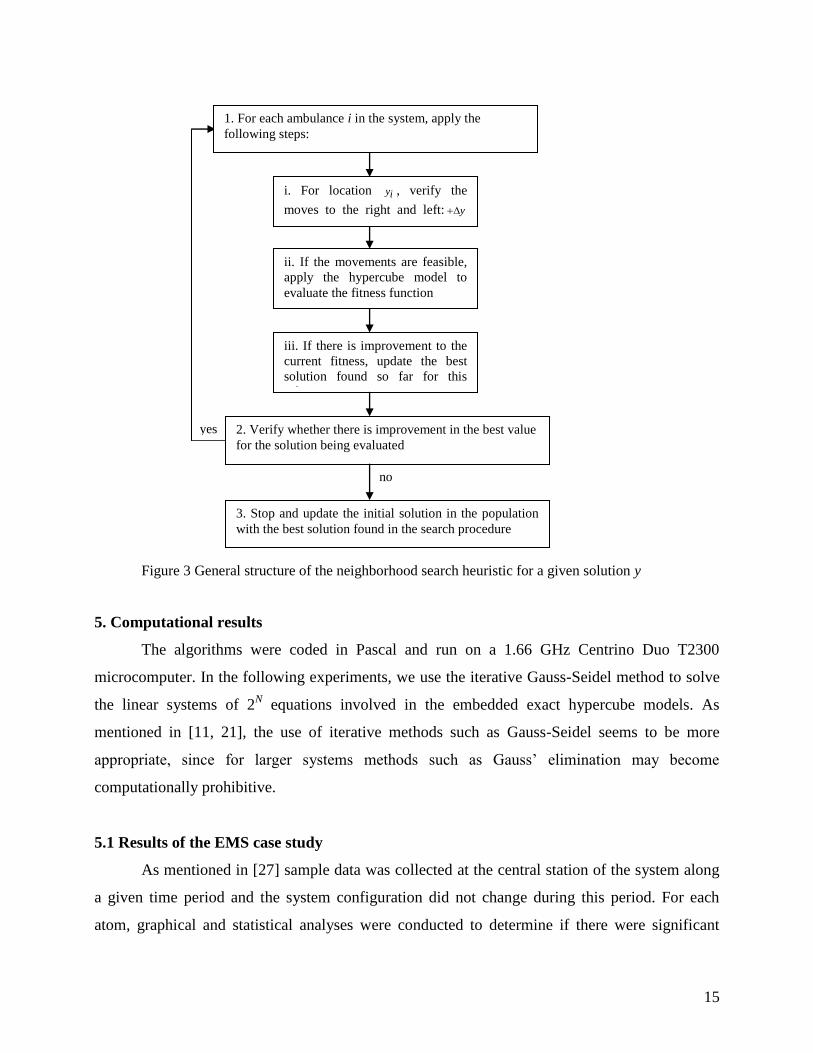
Single-start and multi-start greedy heuristics: we apply a simple single-start greedy

heuristic in order to evaluate the neighborhood of a single solution, which corresponds to the

original configuration of the system being analyzed. We also apply a simple multi-start greedy

algorithm that evaluates the neighborhood of a population of solutions generated according to the

procedures discussed before. In general, in a multi-start greedy heuristic a number of different

initial solutions are generated and typically improved by neighborhood search methods. We

apply both approaches to solve the two problems (location and districting) separately. For

example, considering the location problem, for a given solution y, we apply the following local

search procedure:

(i) For all ambulances i = 1, 2, …, N of the system, we analyze two possible movements: to

the left and the right of their current locations iy , i.e., modifying each location to yyi and

yyi , where y is an input parameter.

14

(ii) In this marginal analysis of each movement of each ambulance i, we preserve the original

location of the other ambulances in the system and we apply either the exact or approximate

hypercube model to evaluate the changes in the fitness function value. If there are improvements,

we update the incumbent solution with the best improvement and we repeat the above procedure;

otherwise, the procedure is finished.

(iii) In order to avoid cycles during the iterations of the procedure, we keep in a simple tabu

list the two best movements achieved in the last two iterations. Before moving to the next

candidate, we not only verify that it is not in the tabu list, but we also check the constraints of

minimum distance ( Dd

ii yy min

1 ) and (0 iy 1), and we evaluate the movement (solving the

hypercube model) only if these conditions are found.

For the districting problem, we follow the same procedure above for each solution x

(considering that each solution is a vector of 1N values, and the constraint 0.2 ix 0.8).

Figure 3 presents the general scheme of this simple local search heuristic. In setting the critical

parameters of these greedy algorithms, such as the precision y and the number of initial

solutions ( Pop - population size to be generated in the multi-start greedy heuristics), we ran

extensive preliminary tests varying the values of these parameters within certain ranges. The set

of values y = 0.005 and Pop = 10 and 20 yielded the best results in most of the tests for both

the location and districting problems, as discussed in section 5.

The evaluation procedure computes the performance measures for each configuration

using either the exact or approximate hypercube model outlined in sections 2 and 3, respectively.

We conducted different experiments to optimize separate measures (fitness function )(xf of

initial solution x) to evaluate each generated configuration. In these experiments, the objective

was to minimize the mean region-wide travel time (i.e., )()(min xTxf ), or to minimize the

fraction of calls not serviced within 10 minutes (i.e., )()(min 10 xPxf t ), or to reduce the

workload imbalance within the fleet by minimizing the standard deviation of server workloads

(i.e., )()(min xxf ).

15

Figure 3 General structure of the neighborhood search heuristic for a given solution y

5. Computational results

The algorithms were coded in Pascal and run on a 1.66 GHz Centrino Duo T2300

microcomputer. In the following experiments, we use the iterative Gauss-Seidel method to solve

the linear systems of 2N equations involved in the embedded exact hypercube models. As

mentioned in [11, 21], the use of iterative methods such as Gauss-Seidel seems to be more

appropriate, since for larger systems methods such as Gauss’ elimination may become

computationally prohibitive.

5.1 Results of the EMS case study

As mentioned in [27] sample data was collected at the central station of the system along

a given time period and the system configuration did not change during this period. For each

atom, graphical and statistical analyses were conducted to determine if there were significant

yes

no

i. For location iy , verify the

moves to the right and left: y

and y

ii. If the movements are feasible,

apply the hypercube model to

evaluate the fitness function

iii. If there is improvement to the

current fitness, update the best

solution found so far for this

solution

1. For each ambulance i in the system, apply the

following steps:

2. Verify whether there is improvement in the best value

for the solution being evaluated

3. Stop and update the initial solution in the population

with the best solution found in the search procedure

16

variations in the call data by month, week and day of the week. These analyses indicated that the

monthly and weekly user arrival rates remained approximately constant during this period, while

the system showed higher service demands on weekends than on workdays. Therefore, the

chosen periods of analysis were weekends. To test the validity of the steady-state assumption,

simulations were run showing that the required warm-up periods were relatively short and that

steady-state assumption would be acceptable for the study.

Results of exact vs. approximate hypercube models applied to the case study: we

applied the hypercube approximations discussed in section 3 to obtain the main performance

measures of the original configuration of the case study: T (mean travel time), 10tP (fraction of

calls not serviced within 10 minutes) and (mean standard deviation of workloads). In Table 1

we compare these results with the results obtained by the exact hypercube model. The original

configuration of the system based on atom size is represented by the vector ),,,,( 54321 xxxxxx

= (0.50, 0.50, 0.50, 0.50, 0.22), and the location of ambulances is represented by the vector y =

(y1, y2, y3, y4, y5, y6) = (0.0, 0.2192, 0.3315, 0.4973, 0.7807, 1.0). The stretch of highway in

Figure 1 is 187 km in length. The workloads calculated by the exact hypercube model are: 1 =

0.1352; 2 = 0.1928; 3 = 0.1612; 4 = 0.3026; 5 = 0.1833 and 6 = 0.1490, and the results

obtained by the approximate hypercube model are 1 = 0.1358; 2 = 0.1945; 3 = 0.1647; 4 =

0.3038; 5 = 0.1821 and 6 = 0.1476. Note in Table 1 that the results obtained by the exact and

approximate models are relatively close.

Table 1 – Results of the exact and approximate hypercube models to the original configuration of

the system

Measure Exact

Model

Approximate

model

%

deviation

T 7.912 7.907 -0.06%

10tP 0.299 0.300 0.33%

0.0551 0.0553 0.36%

Results of single-start and multi-start greedy algorithms: we conducted three

experiments individually optimizing each of the fitness functions discussed in section 4 for both

districting and location problems: )()(min xTxf , )()(min 10 xPxf t , and

17

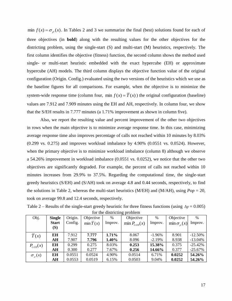
)()(min xxf . In Tables 2 and 3 we summarize the final (best) solutions found for each of

three objectives (in bold) along with the resulting values for the other objectives for the

districting problem, using the single-start (S) and multi-start (M) heuristics, respectively. The

first column identifies the objective (fitness) function, the second column shows the method used

single- or multi-start heuristic embedded with the exact hypercube (EH) or approximate

hypercube (AH) models. The third column displays the objective function value of the original

configuration (Origin. Config.) evaluated using the two versions of the heuristics which we use as

the baseline figures for all comparisons. For example, when the objective is to minimize the

system-wide response time (column four, )()(min xTxf ) the original configuration (baseline)

values are 7.912 and 7.909 minutes using the EH and AH, respectively. In column four, we show

that the S/EH results in 7.777 minutes (a 1.71% improvement as shown in column five).

Also, we report the resulting value and percent improvement of the other two objectives

in rows when the main objective is to minimize average response time. In this case, minimizing

average response time also improves percentage of calls not reached within 10 minutes by 8.03%

(0.299 vs. 0.275) and improves workload imbalance by 4.90% (0.0551 vs. 0.0524). However,

when the primary objective is to minimize workload imbalance (column 8) although we observe

a 54.26% improvement in workload imbalance (0.0551 vs. 0.0252), we notice that the other two

objectives are significantly degraded. For example, the percent of calls not reached within 10

minutes increases from 29.9% to 37.5%. Regarding the computational time, the single-start

greedy heuristics (S/EH) and (S/AH) took on average 4.8 and 0.44 seconds, respectively, to find

the solutions in Table 2, whereas the multi-start heuristics (M/EH) and (M/AH), using Pop = 20,

took on average 99.8 and 12.4 seconds, respectively.

Table 2 – Results of the single-start greedy heuristic for three fitness functions (using y = 0.005)

for the districting problem

Obj. Single

Start

(S)

Origin.

Config.

Objective

)(min xT

%

Improv.

Objective

)(min 10 xPt

%

Improv.

Objective

)(min x

%

Improv.

)(xT EH

AH

7.912

7.907 7.777

7.796

1.71%

1.40%

8.067

8.096

-1.96%

-2.19%

8.901

8.938

-12.50%

-13.04%

)(10 xPt EH

AH

0.299

0.300

0.275

0.277

8.03%

7.67% 0.253

0.256

15.38%

14.66%

0.375

0.377

-25.42%

-25.67%

)(x EH

AH

0.0551

0.0553

0.0524

0.0519

4.90%

6.15%

0.0514

0.0503

6.71%

9.04% 0.0252

0.0252

54.26%

54.26%

18

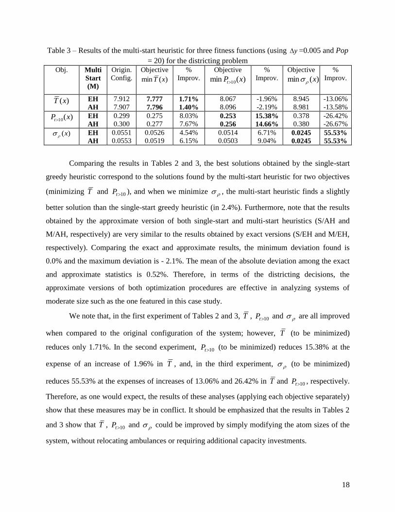
Table 3 – Results of the multi-start heuristic for three fitness functions (using y =0.005 and Pop

= 20) for the districting problem

Obj. Multi

Start

(M)

Origin.

Config.

Objective

)(min xT

%

Improv.

Objective

)(min 10 xPt

%

Improv.

Objective

)(min x

%

Improv.

)(xT EH

AH

7.912

7.907 7.777

7.796

1.71%

1.40%

8.067

8.096

-1.96%

-2.19%

8.945

8.981

-13.06%

-13.58%

)(10 xPt EH

AH

0.299

0.300

0.275

0.277

8.03%

7.67% 0.253

0.256

15.38%

14.66%

0.378

0.380

-26.42%

-26.67%

)(x EH

AH

0.0551

0.0553

0.0526

0.0519

4.54%

6.15%

0.0514

0.0503

6.71%

9.04% 0.0245

0.0245

55.53%

55.53%

Comparing the results in Tables 2 and 3, the best solutions obtained by the single-start

greedy heuristic correspond to the solutions found by the multi-start heuristic for two objectives

(minimizing T and 10tP ), and when we minimize , the multi-start heuristic finds a slightly

better solution than the single-start greedy heuristic (in 2.4%). Furthermore, note that the results

obtained by the approximate version of both single-start and multi-start heuristics (S/AH and

M/AH, respectively) are very similar to the results obtained by exact versions (S/EH and M/EH,

respectively). Comparing the exact and approximate results, the minimum deviation found is

0.0% and the maximum deviation is - 2.1%. The mean of the absolute deviation among the exact

and approximate statistics is 0.52%. Therefore, in terms of the districting decisions, the

approximate versions of both optimization procedures are effective in analyzing systems of

moderate size such as the one featured in this case study.

We note that, in the first experiment of Tables 2 and 3, T , 10tP and are all improved

when compared to the original configuration of the system; however, T (to be minimized)

reduces only 1.71%. In the second experiment, 10tP (to be minimized) reduces 15.38% at the

expense of an increase of 1.96% in T , and, in the third experiment, (to be minimized)

reduces 55.53% at the expenses of increases of 13.06% and 26.42% in T and 10tP , respectively.

Therefore, as one would expect, the results of these analyses (applying each objective separately)

show that these measures may be in conflict. It should be emphasized that the results in Tables 2

and 3 show that T , 10tP and could be improved by simply modifying the atom sizes of the

system, without relocating ambulances or requiring additional capacity investments.

19

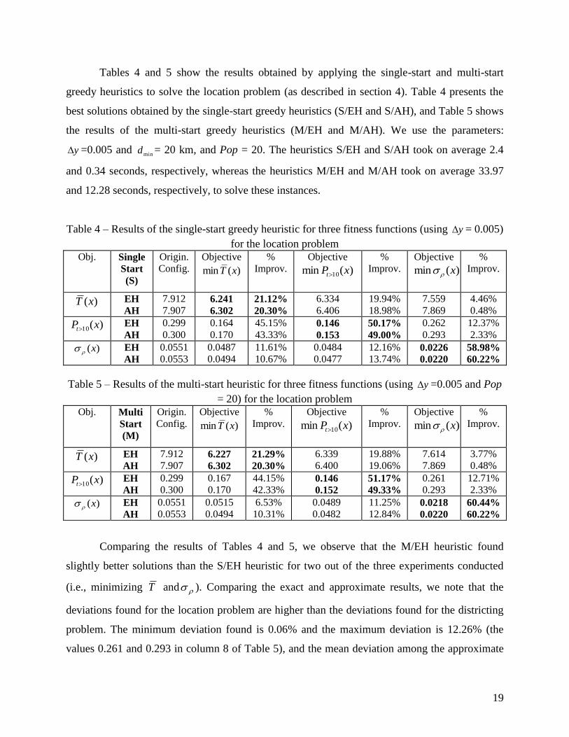
Tables 4 and 5 show the results obtained by applying the single-start and multi-start

greedy heuristics to solve the location problem (as described in section 4). Table 4 presents the

best solutions obtained by the single-start greedy heuristics (S/EH and S/AH), and Table 5 shows

the results of the multi-start greedy heuristics (M/EH and M/AH). We use the parameters:

y =0.005 and min

d = 20 km, and Pop = 20. The heuristics S/EH and S/AH took on average 2.4

and 0.34 seconds, respectively, whereas the heuristics M/EH and M/AH took on average 33.97

and 12.28 seconds, respectively, to solve these instances.

Table 4 – Results of the single-start greedy heuristic for three fitness functions (using y = 0.005)

for the location problem

Obj. Single

Start

(S)

Origin.

Config.

Objective

)(min xT

%

Improv.

Objective

)(min 10 xPt

%

Improv.

Objective

)(min x

%

Improv.

)(xT EH

AH

7.912

7.907 6.241

6.302

21.12%

20.30%

6.334

6.406

19.94%

18.98%

7.559

7.869

4.46%

0.48%

)(10 xPt EH

AH

0.299

0.300

0.164

0.170

45.15%

43.33% 0.146

0.153

50.17%

49.00%

0.262

0.293

12.37%

2.33%

)(x EH

AH

0.0551

0.0553

0.0487

0.0494

11.61%

10.67%

0.0484

0.0477

12.16%

13.74% 0.0226

0.0220

58.98%

60.22%

Table 5 – Results of the multi-start heuristic for three fitness functions (using y =0.005 and Pop

= 20) for the location problem

Obj. Multi

Start

(M)

Origin.

Config.

Objective

)(min xT

%

Improv.

Objective

)(min 10 xPt

%

Improv.

Objective

)(min x

%

Improv.

)(xT EH

AH

7.912

7.907 6.227

6.302

21.29%

20.30%

6.339

6.400

19.88%

19.06%

7.614

7.869

3.77%

0.48%

)(10 xPt EH

AH

0.299

0.300

0.167

0.170

44.15%

42.33% 0.146

0.152

51.17%

49.33%

0.261

0.293

12.71%

2.33%

)(x EH

AH

0.0551

0.0553

0.0515

0.0494

6.53%

10.31%

0.0489

0.0482

11.25%

12.84% 0.0218

0.0220

60.44%

60.22%

Comparing the results of Tables 4 and 5, we observe that the M/EH heuristic found

slightly better solutions than the S/EH heuristic for two out of the three experiments conducted

(i.e., minimizing T and ). Comparing the exact and approximate results, we note that the

deviations found for the location problem are higher than the deviations found for the districting

problem. The minimum deviation found is 0.06% and the maximum deviation is 12.26% (the

values 0.261 and 0.293 in column 8 of Table 5), and the mean deviation among the approximate

20

and corresponding exact statistics is 3.0%. Even so, if we consider only the objective function

values in bold, the results obtained by the approximate version of both heuristics (S/AH and

M/AH) are close to the results obtained by their corresponding exact versions (S/EH and M/EH,

respectively). We note that for the three experiments, T , 10tP and are all improved when

compared to the original configuration of the system. Furthermore, we note that the solutions

obtained for the location problem resulted in higher improvements in the main system

performance measures than the solutions obtained for the districting problem.

5.2 Results of large problem instances

Initially, we examine the performance of the exact and approximate algorithms for other

problem instances slightly larger than the case study of section 2, considering the districting and

location problems. We compare the results obtained by the exact and approximate versions for

testing problems with N = 6, 8, and 10 ambulances (bases), randomly generated, based on the

data set of the EMS case study in [27]. For example, the arrival rate j of each atom j was

randomly generated sorting a value in the interval ( maxmin ,ll ), where minl and maxl are determined

based on the minimum and maximum arrival rates in the case study ( min , max ) as follows:

2)(

minminminmax l and 2

)(maxmax

minmax l . Given that for this case study min = 0.00008

and max =0.00375, we set minl = 0 to avoid negative values for j . Similarly, the service rate i

of each server i was randomly sorted in the interval ( minm , maxm ), where 2)(

minminminmax mm ,

2)(

maxmaxminmax mm , and min = 0.0241 and max = 0.0101 are the minimum and maximum

service rates in the case study.

The initial location of each ambulance i was determined by a procedure similar to the one

described in section 4 to generate the initial solutions of the location multi-start greedy heuristics

(with 01 y and 1Ny ), and the total stretch length D for each instance of N ambulances was

determined as follows: 00)/( DNND , where 0D = 187 (total stretch length of the case study)

and 0N = 6 (number of ambulances in the case study). In addition, we assume that, for these

instances, the size of each atom corresponds to half of the distance between two adjacent bases.

In these experiments we optimize the two objective (fitness) functions discussed in section 3:

)()(min xTxf and )()(min xxf separately.

21

We summarize our findings of the single-start and multi-start greedy heuristics for the

districting and location problems in Tables 6 and 7, respectively. The tables present the objective

function values for the exact (EH) and approximate (AH) versions along with the corresponding

average runtimes. Observe in Table 6 that, for the districting problem, when we minimize )(xT ,

both heuristics find the same solution, whereas when we minimize )(x , the multi-start heuristic

finds better solutions than the single-start heuristic for some experiments albeit at the expense of

higher runtimes. Moreover, the deviations among the exact and approximate solutions in Table 6

are relatively small. The maximum deviation is 1.9%, the minimum deviation is 0.0%, and the

mean deviation is 0.96%.

Observe in Table 7 that, for the location problem, there are experiments for which the

multi-start heuristic finds better solutions than the single-start heuristic, although in the remaining

experiments it provides the same solution. Comparing the exact and approximate solutions of

both heuristics, we note that the deviations in Table 7 (the location problem) are higher than those

in Table 6 (the districting problem). For example, considering all measures in Table 7, the

maximum deviation is –12.6%, the minimum deviation is 0.40%, and the mean deviation is

4.41%, which is acceptable for the decisions involved in real life.

Table 6 – Results of the heuristics for the districting problem (with EH and AH, using y =0.005

and Pop = 20)

Problem

instance

Objective

Original

Config.

Single-

start

Percent

Improv.

Time

(sec)

Multi-

start

Percent

Improv

Time

(sec)

N = 6 )(min xT EH

AH

8.133

8.255

7.471

7.563

8.14%

8.38%

4.24

0.46

7.471

7.563

8.14%

8.38%

118.73

10.20

)(min x

EH

AH

0.1303

0.1293

0.0552

0.0552

57.64%

57.31%

7.14

0.74

0.0539

0.0543

58.63%

58.00%

122.23

14.21

N = 8 )(min xT

EH

AH

7.192

7.267

7.008

7.092

2.56%

2.41%

69.28

1.21

7.008

7.092

2.56%

2.41%

3326.49

29.30

)(min x

EH

AH

0.0824

0.0840

0.0676

0.0679

17.96%

19.17%

160.02

1.33

0.0676

0.0679

17.96%

19.17%

3686.51

36.21

N = 10 )(min xT

EH

AH

7.758

7.799

7.462

7.520

3.81%

3.58%

2314.4

2.25

7.462

7.520

3.81%

3.58%

33843.8

71.29

)(min x

EH

AH

0.1786

0.1798

0.1331

0.1310

25.4!%

27.14%

4536.2

3.44

0.1326

0.1310

25.76%

27.14%

35281.7

74.08

22

Table 7 – Results of the heuristics for the location problem (with EH and AH, using y = 0.005

and Pop = 20)

Problem

instance

Objective

Original

Config.

Single-

start

Percent

Improv.

Time

(sec)

Multi-

start

Percent

Improv

Time

(sec)

N = 6 )(min xT EH

AH

8.133

8.255

5.745

5.576

29.36%

32.45%

1.17

0.38

5.489

5.553

32.51%

32.73%

59.84

11.50

)(min x

EH

AH

0.1303

0.1293

0.0338

0.0304

74.06%

76.49%

1.58

0.58

0.0334

0.0304

74.37%

76.49%

56.42

12.42

N = 8 )(min xT

EH

AH

7.192

7.267

5.739

5.762

20.20%

20.71%

19.30

1.64

5.724

5.762

20.41%

20.71%

230.06

44.11

)(min x

EH

AH

0.0824

0.0840

0.0308

0.0276

62.62%

67.14%

26.90

1.81

0.0303

0.0276

63.23%

67.23%

176.14

18.72

N = 10 )(min xT

EH

AH

7.758

7.799

6.350

5.860

18.15%

24.86%

363.39

1.82

5.832

5.860

24.83%

24.86%

2218.31

61.03

)(min x

EH

AH

0.1786

0.1798

0.1286

0.1176

27.99%

34.59%

306.12

2.32

0.1162

0.1015

34.94%

43.55%

2431.57

42.06

It is important to emphasize that, even using an iterative method to solve the linear

systems of the hypercube model, the computer runtime requirements of the optimization

procedures using the exact hypercube model increase significantly for N 10 ambulances. In

contrast, the approximate versions of the algorithm require much less computational effort to find

ambulance locations and atom sizes with reasonably small deviation from the exact solutions.

Next, we investigate the use the optimization procedures to analyze much larger problem

instances, which are randomly generated as before with sizes varying from 12 to 100 ambulances.

Indeed, there are highway EMS systems in Brazil with relatively large number of ambulances.

For example, in Sao Paulo state there are systems with more than 20 ambulances (e.g., the EMS

Nova Dutra, run by a private firm contracted by the government to operate on the highway

linking the cities of Sao Paulo and Rio de Janeiro). Moreover, the methods we propose could be

extended for urban EMS usage, which usually corresponds to large systems in moderate to large

cities. For instance, the SAMU system in the urban area of Sao Paulo has more than 50

ambulance bases (with a total of more than 130 ambulances operating 24 hours per day).

The results for the objective function of each solution are presented in Tables 8 and 9 for

the districting and location problems, respectively. Note that in these cases we do not apply the

exact versions of the algorithms because of the high computational efforts required. For example,

for a system with N = 20 ambulances, the number of equations is 220

, which is in excess of one

23

million. In the following experiments we used y = 0.005 for both greedy heuristics and Pop = 20

for the multi-start heuristic.

Table 8 – Results of the heuristics for the districting problem

Problem

instance

Objective Original

Config.

Single-

start

Percent

Improv.

Time

(sec)

Multi-

start

Percent

Improv

Time

(sec)

N = 12 )(min xT 7.593 7.163 5.66% 4.24 7.163 5.66% 131.58

)(min x 0.1226 0.0791 35.48% 7.47 0.0787 35.81% 163.02

N = 18 )(min xT 6.985 6.864 1.73% 8.84 6.864 1.73% 488.67

)(min x 0.1133 0.0813 28.24% 27.89 0.0810 28.24% 584.64

N = 24 )(min xT 7.027 6.750 3.94% 28.36 6.750 3.94% 1123.22

)(min x 0.1206 0.0905 24.96% 62.89 0.0901 25.29% 1694.89

N = 30 )(min xT 7.038 6.809 3.25% 57.53 6.809 3.25% 2534.08

)(min x 0.1195 0.0851 28.79% 139.65 0.0848 29.04% 3162.81

N = 36 )(min xT 6.843 6.686 2.29% 82.89 6.686 2.29% 3496.44

)(min x 0.1024 0.0749 26.85% 265.65 0.0746 27.15% 5812.19

N = 42 )(min xT 6.774 6.641 1.96% 137.71 6.641 1.96% 6410.55

)(min x 0.1008 0.0673 33.23% 442.47 0.0670 33.53% 8769.15

N = 50 )(min xT 6.962 6.788 2.50% 304.72 6.788 2.50% 8133.97

)(min x 0.1475 0.1136 22.98% 756.90 0.1132 23.25% 9658.17

N = 60 )(min xT 6.944 6.814 1.87% 439.59 6.814 1.87% 15339.04

)(min x 0.1342 0.1062 20.86% 1344.16 0.1060 21.01% 23179.55

N = 100 )(min xT 6.866 6.642 3.26% 3356.28 6.638 3.32% 25379.65

)(min x 0.1386 0.1070 22.80% 7490.33 0.1068 22.94% 30998.43

Results in Table 8 suggest a few generalizations. We note that similar to the findings from the

experiments for the districting problem in section 5.1 the percentage of improvements when

minimizing T are smaller than the improvement when the objective is to minimize p . By

comparing the results of the single-start greedy heuristic with the multi-start greedy heuristic, we

observe that when minimizing T , there is very little to no improvement in the solution quality

when we switch from single-start to multi-start. Hence, if the objective is to minimize T single-

start approach will solve quickly and generate high quality solutions. If the objective is to

minimize p , the multi-start greedy heuristic found slightly better solutions than the single-start

greedy heuristic, however, these improvements came at the expense of much higher runtime

requirements.

24

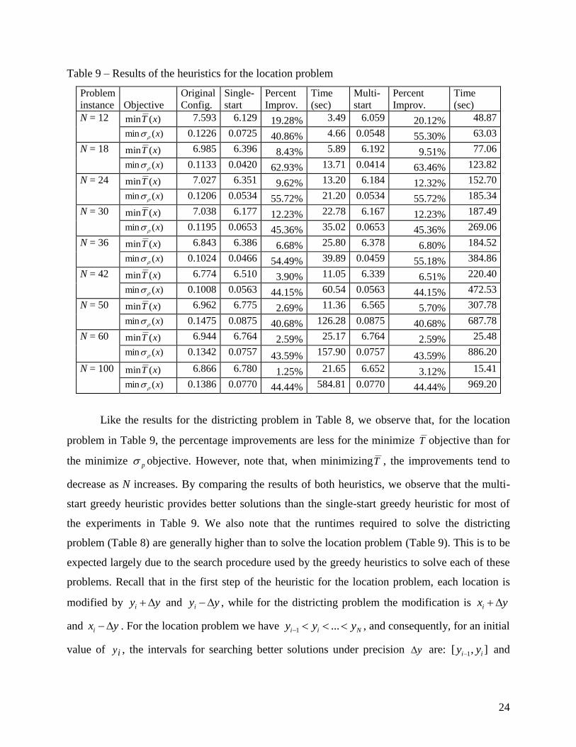
Table 9 – Results of the heuristics for the location problem

Problem

instance

Objective

Original

Config.

Single-

start

Percent

Improv.

Time

(sec)

Multi-

start

Percent

Improv.

Time

(sec)

N = 12 )(min xT 7.593 6.129 19.28% 3.49 6.059 20.12% 48.87

)(min x 0.1226 0.0725 40.86% 4.66 0.0548 55.30% 63.03

N = 18 )(min xT 6.985 6.396 8.43% 5.89 6.192 9.51% 77.06

)(min x 0.1133 0.0420 62.93% 13.71 0.0414 63.46% 123.82

N = 24 )(min xT 7.027 6.351 9.62% 13.20 6.184 12.32% 152.70

)(min x 0.1206 0.0534 55.72% 21.20 0.0534 55.72% 185.34

N = 30 )(min xT 7.038 6.177 12.23% 22.78 6.167 12.23% 187.49

)(min x 0.1195 0.0653 45.36% 35.02 0.0653 45.36% 269.06

N = 36 )(min xT 6.843 6.386 6.68% 25.80 6.378 6.80% 184.52

)(min x 0.1024 0.0466 54.49% 39.89 0.0459 55.18% 384.86

N = 42 )(min xT 6.774 6.510 3.90% 11.05 6.339 6.51% 220.40

)(min x 0.1008 0.0563 44.15% 60.54 0.0563 44.15% 472.53

N = 50 )(min xT 6.962 6.775 2.69% 11.36 6.565 5.70% 307.78

)(min x 0.1475 0.0875 40.68% 126.28 0.0875 40.68% 687.78

N = 60 )(min xT 6.944 6.764 2.59% 25.17 6.764 2.59% 25.48

)(min x 0.1342 0.0757 43.59% 157.90 0.0757 43.59% 886.20

N = 100 )(min xT 6.866 6.780 1.25% 21.65 6.652 3.12% 15.41

)(min x 0.1386 0.0770 44.44% 584.81 0.0770 44.44% 969.20

Like the results for the districting problem in Table 8, we observe that, for the location

problem in Table 9, the percentage improvements are less for the minimize T objective than for

the minimize p objective. However, note that, when minimizingT , the improvements tend to

decrease as N increases. By comparing the results of both heuristics, we observe that the multi-

start greedy heuristic provides better solutions than the single-start greedy heuristic for most of

the experiments in Table 9. We also note that the runtimes required to solve the districting

problem (Table 8) are generally higher than to solve the location problem (Table 9). This is to be

expected largely due to the search procedure used by the greedy heuristics to solve each of these

problems. Recall that in the first step of the heuristic for the location problem, each location is

modified by yyi and yyi , while for the districting problem the modification is yxi

and yxi . For the location problem we have Nii yyy ...1 , and consequently, for an initial

value of iy , the intervals for searching better solutions under precision y are: ],[ 1 ii yy and

25

],[ 1ii yy . In addition, each attempt is constrained to ( Dd

ii yy min

1 ) and (0 iy 1). In

contrast, for the districting problem, for an initial value of ix the intervals are: ],2.0[ ix and

]8.0,[ ix , which increase the search space compared to the location problem, and consequently,

the computational time required by the search procedure is higher.

6. Conclusions

In this paper, we present simple and straightforward greedy heuristic algorithms to

optimize the configuration and operation of large-scale EMS on highways. The main drawback of

previous approaches has been excessive computing requirements in part due to using exact

hypercube queuing models integrated into optimization procedures. We overcome these obstacles

with a straightforward algorithm which utilizes a fast and accurate hypercube approximation

method developed by Atkinson et al. [1]. The algorithms can be effective tools to support design

and operational decisions in these systems, for example, to determine the best locations of

ambulances and/or the best district sizes for a given system configuration so that the mean user

response time and the ambulances’ workload imbalances are minimized. The proposed

approaches are practical alternatives for the analysis of these systems, providing reasonable

accuracy and affordable running times.

We first tested our approaches on a well-documented case study of an EMS on a Brazilian

highway and then constructed a series of experiments with much larger problem instances with

the number of ambulances N varying up to 100. For the location and districting problems

analyzed, different system performance measures, such as the mean user response time, fraction

of calls not reached within 10 minutes, and the workload imbalance among the ambulances, were

improved by applying the methods. For example, for the districting problem, these performance

measures were improved by simply modifying the atom sizes of the system without relocating

ambulances and without requiring additional capacity investments. By using these methods for

relocating the ambulances of the system, the improvements in the performance measures (e.g.,

the mean region wide response time) were even higher than those achieved by solving the

districting problem.

26

An interesting perspective for future research is the refinement of the multi-start greedy

algorithms, for example, improving the procedures involved in generating the initial population.

Another line of research is the extension of the location and districting heuristic algorithms to

deal with EMS on highways involving different operational policies (e.g., different dispatch

preference lists, multiple dispatches of ambulances, and dynamic relocation of ambulances).

Finally, the methods could be extended to examine urban EMS, which usually correspond to

large systems in moderate to large cities, and deployment response systems to terrorist attacks

and other major emergencies.

References

[1] Atkinson JB, Kovalenko IN, Kuznetsov N, Mykhalevych KV. Heuristic solution methods for a

hypercube queuing model of the deployment of emergency systems. Cybernetics and Systems

Analysis 2006;42(3):379-391.

[2] Atkinson JB, Kovalenko IN, Kuznetsov N, Mykhalevych KV. A hypercube queuing loss model

with customer-dependent service rates. European Journal of Operational Research

2008;191(1):223-239.

[3] Ball MO, Lin LF. A reliability model applied to emergency service vehicle location. Operations

Research 1993;41:18-36.

[4] Batta R, Dolan JM, Krishnamurthy NN. The maximal expected covering location problem:

Revisited. Transportation Science 1989;23:277-287.

[5] Berman O. Dynamic positioning of mobile servers on networks. in MIT Operations Research

Center. 1978, MIT Operations Research Center: Cambridge, Mass.

[6] Brandeau M, Larson RC, Extending and applying the hypercube queuing model to deploy

ambulances in boston. In: Delivery of urban services, A.J. Swersey and E.J. Ingnall, Editors.

1986, Elsevier. p. 121-123.

[7] Bronmo G, Christiansen M, Fagerholt K, Nygreen B. A multi-start local search heuristic for ship

scheduling - a computational study. Computers & Operations Research 2007;34:900-917.

[8] Budge S, Ingolfsson A, Erkut E. Approximating vehicle dispatch probabilities for emergency

service systems with location-specific service times and multiple units per location. Operations

Research 2008;In press.

[9] Burwell T, Jarvis JP, McKnew MA. Modeling co-located servers and dispatch ties in the

hypercube model. Computers & Operations Research 1993;20:113-119.

27

[10] Chelst K, Barlach Z. Multiple unit dispatches in emergency services: Models to estimate system

performance. Management Science 1981;27(12):1390-1409.

[11] Chiyoshi FY, Galvao RD, Morabito R. A note on solutions to the maximal expected covering

location problem. Computers & Operations Research 2002;30:87-96.

[12] Galvao RD, Chiyoshi FY, Morabito R. Towards unified formulations and extensions of two

classical probabilistic location models. Computers & Operations Research 2005;32(1):15-33.

[13] Galvao RD, Morabito R. Emergency service systems: The use of the hypercube queueing model

in the solution of probabilistic location problems. International Transactions in Operation

Research 2008;15:1-25.

[14] Goldberg DE, Szidarovszky F. Methods for solving nonlinear equations used in evaluating

emergency vehicle busy probabilities. Operations Research 1991;39(6):903-916.

[15] Iannoni AP, Morabito R. A multiple dispatch and partial backup hypercube queuing model to

analyze emergency medical systems on highways. Transportation Research Part E 2007;43:775-

771.

[16] Iannoni AP, Morabito R, Saydam C. A hypercube queueing model embedded into a genetic

algorithm for ambulance deployment on highways. Annals of Operations Research 2008;157:207-

224.

[17] Iannoni AP, Morabito R, Saydam C. An optimization approach for ambulance location and the

districting of the response segments on highways. European Journal of Operational Research

2009;195(2):528-542.

[18] Ingolfsson A, Budge S, Erkut E. Optimal ambulance location with random delays and travel

times. Health Care Management Science 2008;11(3):262-274.

[19] Jarvis JP. Approximating the equilibrium behavior of multi-server loss systems. Management

Science 1985;31:235-239.

[20] Lan G, DePuy GW. On the effectiveness of incorporating randomness and memory into a multi-

start metaheuristic with application to the set covering problem. Computers & Industrial

Engineering 2006;51:362-374.

[21] Larson RC. A hypercube queuing model for facility location and redistricting in urban emergency

services. Computers & Operations Research 1974;1:67-95.

[22] Larson RC. Approximating the performance of urban emergency service systems. Operations

Research 1975;23:845-868.

[23] Larson RC, Structural system models for locational decisions: An example using the hypercube

queueing model. In: Operational research ’78, K.B. Haley, Editor. 1979, North-Holland

Publishing Co.: Amsterdam, Holland. p. 1054-1091.

28

[24] Larson RC. Urban operations research. Englewood Cliffs, N.J: Prentice-Hall; 1981.

[25] Larson RC. O.R. Models for homeland security. ORMS Today 2004;31:22-29.

[26] Martin R, Multi-start methods. In: Handbook of metaheuristics., F.W. Glover and G.A.

Kochenberger, Editors. 2003, Springer: Berlin. p. 355-368.

[27] Mendonça FC, Morabito R. Analyzing emergency service ambulance deployment on a brazilian

highway using the hypercube model. Journal of the Operational Research Society 2001;52:261-

270.

[28] Morabito R, Chiyoshi F, Galvao R. Non-homogeneous servers in emergency medical systems:

Practical applications using the hypercube queueing model. Socio-Economic Planning Sciences

2008;42:255-270.

[29] Rajagopalan HK, Saydam C, Xiao J. A multiperiod set covering location model for dynamic

redeployment of ambulances. Computers & Operations Research 2008;35:814-826.

[30] Resende MGC, Werneck RF. A hybrid heuristic for the p-median. Problem. Journal of Heuristics

2004;10(1):59-88.

[31] Resende MGC, Werneck RF. A hybrid multi-start heuristic for the uncapacitated facility location

problem. European Journal of Operational Research 2006;174:54-68.

[32] Sacks SR, Grief S. Orlando police department uses or/ms methodology, new software to design

patrol districts. ORMS Today 1994;21:30-32.

[33] Saydam C, Aytug H. Accurate estimation of expected coverage: Revisited. Socio-Economic

Planning Sciences 2003;37:69-80.

[34] Takeda RA, Widmer JA, Morabito R. Analysis of ambulance decentralization in an urban medical

emergency service using the hypercube queuing model. Computers & Operations Research

2007;34:727-741.

29

Ana Paula Iannoni is a post-doc researcher at Laboratoire Genie Industriel, Ecole

Centrale Paris, France. She received her B. S. and Ph. D. in production engineering from Federal

University of Sao Carlos, Brazil. She was a visiting Ph.D. student at Belk College of Business,

University of North Carolina at Charlotte and held a post-doc at Production Engineering

Department, Federal University of Sao Carlos. Her research interests lie in queuing theory,

simulation and probabilistic location problems applied to emergency medical systems, and

operations research applied to logistics and transportation systems. Dr. Iannoni’s work has

appeared in Transportation Research, Annals of Operational Research, and European Journal of

Operational Research.

Reinaldo Morabito is Associate Professor, Production Engineering Department,

Federal University of Sao Carlos, Brazil. He earned a B.S. in civil engineering from State

University of Campinas, an M.Sc. in operations research and a Ph.D. in transportation

engineering, both from University of Sao Paulo, Brazil. He was a visiting scholar at the Sloan

School of Management, M.I.T., Cambridge, MA. His research interests lie in primarily cutting

and packing problems, lot sizing and scheduling problems, queuing networks applied to

manufacturing systems, probabilistic location problems, and logistics and transportation

planning. His refereed work has appeared in a variety of journals, including Annals of Operations

Research, Asia-Pacific Journal of Operational Research, Canadian Journal of Operational

Research and Information Processing, Computers and Industrial Engineering, Computers and

Operations Research, European Journal of Operational Research, International Journal of

Production Research, International Transactions in Operational Research, Journal of the

Operational Research Society, Production and Operations Management, Socio-Economic

Planning Sciences and Transportation Research.

Cem Saydam is Professor of Operations Management, Belk College of Business,

University of North Carolina at Charlotte. He received his B.S. degree in industrial engineering

from Boğaziçi University, Turkey, and his Ph.D. in engineering management from Clemson

University, Clemson, SC. His teaching and research interests lie in primarily applied

mathematical modeling of emergency response services and operations management applied to

industrial firms. Professor Saydam has published articles in a variety of journals including Socio-

Economic Planning Sciences, Decision Sciences, Computers and Operations Research, European

Journal of Operational Research, Annals of Operations Research, Journal of Operations

Management, and International Journal of Production Research. He is a member of INFORMS

and Decision Sciences Institute.