Optimizing a constrained convex polygonal annulus

a

lus

awa,

SA

ms forology

thishe inner

izings to aoints.

ither thetationsfinding

and by

Canada

Journal of Discrete Algorithms 3 (2005) 1–26

www.elsevier.com/locate/jd

Optimizing a constrained convex polygonal annu

Gill Barequeta,∗,1, Prosenjit Boseb,2, Matthew T. Dickersonc,3,Michael T. Goodrichd,4

a Center for Graphics and Geometric Computing, Department of Computer Science,The Technion—Israel Institute of Technology, Haifa 32000, Israel

b School of Computer Science, Carleton University, Herzberg Room 5302, 1125 Colonel By Drive, OttOntario, Canada K1S 5B6

c Department of Mathematics and Computer Science, Middlebury College, Middlebury, VT 05753, Ud Center for Algorithm Engineering, Department of Computer Science, Johns Hopkins University,

Baltimore, MD 21218, USA

Available online 3 February 2004

Abstract

In this paper we give solutions to several constrained polygon annulus placement probleoffset and scaled polygons, providing new efficient primitive operations for computational metrand dimensional tolerancing. Given a convex polygonP and a planar point setS, the goal is to find thethinnest annulus region ofP containingS. Depending on the application, there are several waysproblem can be constrained. In the variants that we address the size of the polygon defining t(respectively, outer) boundary of the annulus is fixed, and the annulus is minimized by minim(respectively, maximizing) the outer (respectively, inner) boundary. We also provide solutionrelated known problem: finding the smallest homothetic copy of a polygon containing a set of pFor all of these problems, we solve for the cases where smallest and largest are defined by eoffsetting or scaling of a polygon. We also provide some experimental results from implemenof several competing approaches to a primitive operation important to all the above variants:the intersection ofn copies of a convex polygon. 2003 Elsevier B.V. All rights reserved.

* Corresponding author.E-mail addresses:[email protected] (G. Barequet), [email protected] (P. Bose),

[email protected] (M.T. Dickerson), [email protected] (M.T. Goodrich).1 Work of this author was supported in part by the Fund for the Promotion of Research at the Technion

a Fialkow Academic Lectureship.2 Work of this author was supported by the Natural Science and Engineering Research Council of

under grant OGP0183877.3 Work of this author was supported by NSF Grants CCR-9902032 and CCR-9732300.4 Work of this author was supported by NSF Grants CCR-9732300 and PHY-9980044.

1570-8667/$ – see front matter 2003 Elsevier B.V. All rights reserved.
doi:10.1016/j.jda.2003.12.004
http://www.elsevier.com/locate/jda

2 G. Barequet et al. / Journal of Discrete Algorithms 3 (2005) 1–26

Keywords:Offset; Annuli; Tolerancing; Optimization

re fo-”, and

rmin-

ng ma-straintsly andraints. Effi-in the,s the

manywidthtesting

nnulusimalityn

, thesedds of

lnulus

nceebeennce

1. Introduction

The research areas of computational metrology and dimensional tolerancing acused on developing repertories of basic tests, such as for “roundness”, “flatnessangle conformity, so as to build a systematic collection of efficient methods for deteing if manufactured parts conform to their design specifications[29,33]. After a part ismanufactured, its surface is sampled by a device known as a coordinate measurichine (CMM) and these sampled points are then tested against various design conto see if this part is conforming or not. The collection of tests that can be done simpefficiently is therefore a limiting factor on the richness and sophistication of the constthat designers can specify with confidence that their designs will be faithfully testedcient methods for several computational-metrology primitives have been presentedalgorithms and computational-geometry literatures (see, e.g.,[1,8,10,12,14–16,24,25,2730–32,34]). This paper provides methods for testing how well a set of points matcheboundary of a convex polygon.

1.1. Offset polygons and their properties

Computing optimal placements of annulus regions is a fundamental aspect ofcomputational metrology tests for quality control in manufacturing. For example, theof the thinnest circular annulus containing a set of points is the measure used for“roundness” by the American National Standards Institute (see[17, pp. 40–42]) and by theInternational Standards Organization. The usual goal is to find, for a certain type of aregion, a placement of the annulus that contains a given set or subset of points. Optof the placement can be measured either byminimizing the size of the annulus regionecessary to contain all (or a certain number) of the points, or bymaximizingthe numberof points contained in a fixed-size annulus. In addition to the tolerancing applicationsproblems also arise in pattern matching and robot localization[18]. Thus we are interestein extending the collection of simple and efficient tolerancing tests to include new kinminimum or maximum annulus placement constraints.

One set of such problems studied recently by Barequet et al. in[5] involves the optimaplacement ofpolygonalannulus regions. These authors noted that the polygonal ancan be defined as the difference region between twoscaledconcentric copies or twooffsetcopies of a convex polygonP . The scaled polygons correspond to the convex distafunctions (also called Minkowski functionals[20, p. 15]), which are extensions of thnotion of scaling circles (in the Euclidean case) to convex polygons. There haveseveral papers (e.g.,[13,23,26]) which explore the Voronoi diagram based on these distafunctions.

Let us define formally the offset of a convex polygon. A convex polygonP is the in-tersection of a collection of closed halfplanes{Hi}, each defined by an edge ofP . Theoffset polygon is the intersection of{Hi(ε)}, whereHi(ε) is the halfplane parallel toHi

G. Barequet et al. / Journal of Discrete Algorithms 3 (2005) 1–26 3

with bounding line translated by distanceε. Positive (respectively, negative) values ofε

well

al-axisut the

lforst theleton

nd we

thatithmsgrams.msg dis-l thanr of apro-

morescaledet op-ementis dis-asr the

. Most

nvext withecisionplace-ation,

er ofnnuluspply ag theualityside

stand for translating the edges outward (respectively, inward) from the polygon. It isknown that the offset operation moves the polygon vertices along themedial axisof thepolygon, so that an edge “disappears” when two polygon vertices meet on a medivertex. (This happens only when the polygon is offset inward.) We denote throughopaper the medial axis of a polygonP by MA(P ).

This offset operation was studied by Aichholzer et al.[3,4] in the context of a novepolygon skeleton, called thestraight skeleton. They discussed the straight skeletonboth convex and simple polygons. For convex polygons the straight skeleton is juwell-known medial axis. For nonconvex simple polygons, however, the straight skeand the medial axis are different. In this paper we deal with convex polygons only, awill refer to the offset skeleton as the polygon medial axis.

Barequet et al.[6] also studied the polygon-offset operation in a different context:of a new distance function and its related Voronoi diagram. They give efficient algorfor computing compact representations of the nearest- and furthest-neighbor diaPolygon offsets were also used in the solution to various annulus placement proble[5].In many applications, including those dealing with manufacturing processes, definintance in terms of an offset from a polygon (either inward or outward) is more naturascaling. This preference for offsetting is motivated by the fact that the absolute erroproduction tool (milling head, laser beam, etc.) is independent of the location of theduced feature relative to some artificial reference point (the origin). Thus, a tool islikely to allow (and expect) local errors bounded by some tolerance, rather thanerrors relative to some (arbitrary) center. For this reason, a study of the polygon-offseration, of the related distance function and its Voronoi diagram, and of annulus-placproblems for offset polygons, are particularly interesting. Theoretical aspects of thtance function and Voronoi diagram were studied in[6], and were used in that paperwell as in[5] in solutions to the offset versions of several problems involving one oother definitions of optimization given above.

1.2. Related results

In [5] several annulus placement problems are solved based on offset polygonsof the problems involved optimizing the placement by fixingδ (the width of the annulusregion) and maximizing the number of points contained. Algorithms are given for coand for simple polygons, and for translation only, as well as for a general placementranslation and rotation allowed. In that paper the authors also solve some related dproblems including an on-line variant. It is suggested that this approach to annulusment may provide a robust solution to various problems that arise in robot localizwith the presence of “noisy data” that need not be contained in the best placement.

As was noted earlier, a related optimization problem is fixing the minimum numbpoints to be contained (sometimes the entire set) and minimizing the size of the aneeded to contain those points. One approach to minimizing the annulus is to aconstraint that either the inner or outer boundary of the annulus is of fixed size. Fixinsize of the inner or outer boundary of an annulus is itself an important aspect of qcontrol. Consider, for example, manufacturing a part (like a cylinder) that must fit in


a corresponding manufactured sleeve. For the part that must fit inside the sleeve, the outersleeve

ientlyt of axingn by

ser-

blemst” weforpoly-

ems:

eus

eus

ef-t

ant of

t

boundary defining the annulus has an absolute maximum which is fixed. For theitself, however, it is the inner boundary that is crucial and must be fixed.

For the case where the annulus boundary is circular, it is shown in[8] that when theinner or outer circle is of fixed size, the placement problem can be solved more efficthan for the general annulus minimization problem. Likewise, we seek a placemenpolygonalannulus region that contains all points, but we follow the same idea of fione boundary of the annulus and minimizing the width (or tolerance) of the regiooffsetting or scaling the other boundary. In particular, we extend the approach of[8] topolygonal annulus regions, and also present some new approaches.

1.3. Problem statements

Throughout this paper we will have a setS of n points and a convex polygon whocomplexity ism. We will omit the definitions ofm andn wherever they are clearly undestood from the context.

In this paper we explore a new set of convex-polygon annulus placement prowhere one of the two annulus boundaries (inner or outer) is fixed. (By a “placemenmean atranslationof the annulus, where no rotation is allowed.) We solve problemspolygonal annulus regions defined for both the polygon-offset and the regular convexgon scaling distance function. In particular, we give algorithms for the following probl

Problem 1. Given a convex polygonP and a set of pointsS, find the largest possiblpolygonP ∗—an inner offset (or a scaled version) ofP —and a placement of the annuldefined byP andP ∗, such that all the points inS are covered by the annulus.

Problem 2. Given a convex polygonP and a set of pointsS, find the smallest possiblpolygonP ∗—an outer offset (or a scaled version) ofP —and a placement of the annuldefined byP andP ∗, such that all the points inS are covered by the annulus.

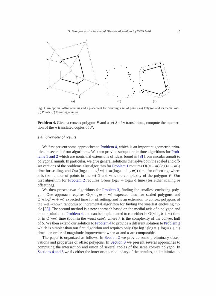
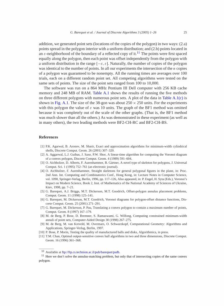
Fig. 1(a)shows a sample polygonP (solid) and an outer offset of it (dashed). For rerence, MA(P ) (the medial axis ofP ) is also shown in light lines.Fig. 1(b)shows a seof pointsS. Fig. 1(c)shows a solution toProblem 2for the givenP andS. That is, wesee an annulus region containing all the points ofS, whose fixed inner boundary isP andwhose outer boundary is the smallest possible offset ofP such thatS can be contained inthe annulus.

The following problem can be viewed as a special case ofProblem 2, when the innerpolygon (the polygon defining the inner boundary of the annulus) is null, or as a varithe famous “smallest enclosing circle” problem for convex polygons:

Problem 3. Given a convex polygonP and a set of pointsS, find the smallest offse(respectively, scaled) translation ofP containing all the points inS.

A substep of several approaches to the above problems is the following:


al axis.

c-

-

d off-

r

y-nds of

g cir-on and

ll

r-to

on. Ine its

(a) (b) (c)

Fig. 1. An optimal offset annulus and a placement for covering a set of points. (a) Polygon and its medi(b) Points. (c) Covering annulus.

Problem 4. Given a convex polygonP and a setS of n translations, compute the intersetion of then translated copies ofP .

1.4. Overview of results

We first present some approaches toProblem 4, which is an important geometric primitive in several of our algorithms. We then provide subquadratic-time algorithms forProb-lems 1 and 2which are nontrivial extensions of ideas found in[8] from circular annuli topolygonal annuli. In particular, we give general solutions that solve both the scaled anset versions of the problems. Our algorithm forProblem 1requires O((n+m) log(n + m))

time for scaling, and O(n(logn + log2 m) + m(logn + logm)) time for offsetting, wheren is the number of points in the setS andm is the complexity of the polygonP . Ourfirst algorithm forProblem 2requires O(nm(logn + logm)) time (for either scaling ooffsetting).

We then present two algorithms forProblem 3, finding the smallest enclosing polgon. One approach requires O(n logm + m) expected time for scaled polygons aO(n log2 m + m) expected time for offsetting, and is an extension to convex polygonthe well-known randomized incremental algorithm for finding the smallest enclosincle [36]. The second method is a new approach based on the medial axis of a polygon our solution toProblem 4, and can be implemented to run either in O(n logh + m) timeor in O(nm) time (both in the worst case), whereh is the complexity of the convex huof S. We then extend our solution toProblem 4to provide a different solution toProblem 2which is simpler than our first algorithm and requires only O(n logn(logn + logm) + m)

time—an order of magnitude improvement whenm andn are comparable.The paper is organized as follows. InSection 2we provide some preliminary obse

vations and properties of offset polygons. InSection 3we present several approachescomputing the intersection and union of several copies of the same convex polygSections 4 and 5we fix either the inner or outer boundary of the annulus, and minimiz


width. InSection 6we investigate further the problem of minimizing the polygon enclosinghe.

ties of

e point.lygon.h the

of theclet, so wepriate

n

ionpped

relatedknowne in-

ld trueis thatnovenality,ronoiwhichhaped) de-et is

wski)

t-n, these

nnected

a given set of points. InSection 7we describe an alternative algorithm for minimizing tannulus with a fixed inner boundary. We end inSection 8with some concluding remarks

2. Preliminary observations

In this section we present both some terminology and some additional properthe polygon-offset distance function. We first define what we mean by aplacementof apolygon. Throughout the paper we assume that each polygon has a fixed referencFor scaled polygons it is natural to assume the center of scaling is contained in the poFor offset polygons the natural reference is the offsetting center: the point to whicinner polygon collapses when the polygon is offset inward. (This point is the centermedial axis of the polygon[6].) In other words, this point is the center of the largest circontained in the polygon. In degenerate cases the offset center can be a segmenarbitrarily select a point in it as the center. (The median of the segment is an approchoice.) By translating a copy of the polygonP to some pointq, we mean the translatioof P that maps its center (reference point) toq. Similarly, when we speak of thereflectionof P , we mean the rotation ofP by π around its center point. The translation of a reflectof P to a pointq translates the polygon so that the center of the reflected copy is mato q.

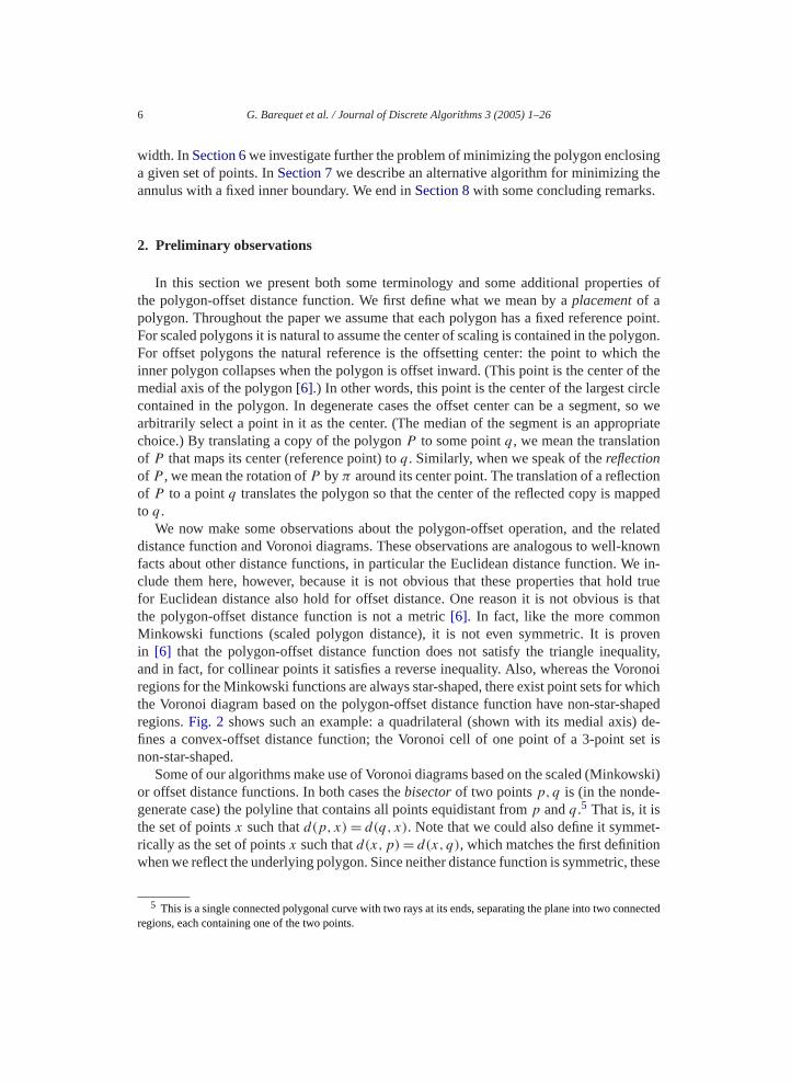
We now make some observations about the polygon-offset operation, and thedistance function and Voronoi diagrams. These observations are analogous to well-facts about other distance functions, in particular the Euclidean distance function. Wclude them here, however, because it is not obvious that these properties that hofor Euclidean distance also hold for offset distance. One reason it is not obviousthe polygon-offset distance function is not a metric[6]. In fact, like the more commoMinkowski functions (scaled polygon distance), it is not even symmetric. It is prin [6] that the polygon-offset distance function does not satisfy the triangle inequand in fact, for collinear points it satisfies a reverse inequality. Also, whereas the Voregions for the Minkowski functions are always star-shaped, there exist point sets forthe Voronoi diagram based on the polygon-offset distance function have non-star-sregions.Fig. 2 shows such an example: a quadrilateral (shown with its medial axisfines a convex-offset distance function; the Voronoi cell of one point of a 3-point snon-star-shaped.

Some of our algorithms make use of Voronoi diagrams based on the scaled (Minkoor offset distance functions. In both cases thebisectorof two pointsp,q is (in the nonde-generate case) the polyline that contains all points equidistant fromp andq.5 That is, it isthe set of pointsx such thatd(p,x) = d(q, x). Note that we could also define it symmerically as the set of pointsx such thatd(x,p) = d(x, q), which matches the first definitiowhen we reflect the underlying polygon. Since neither distance function is symmetric

5 This is a single connected polygonal curve with two rays at its ends, separating the plane into two coregions, each containing one of the two points.


and

e bi-lly

ies oftion(pointat the

es, the

ithms.ee

ontain

Fig. 2. A non-star-shaped Voronoi cell of a point (for the offset distance function).

two definitions result in different bisectors. However, all of the following observationslemmas hold regardless of which definition is used.

Observation 1 (Scale and offset).The bisector between two pointsp and q has ame-dian segments that contain all points that are equidistant fromp and q and such thatthis distance is the minimum of all points on the bisector. In both directions along thsector away froms, distances fromp and q to points on the bisector are monotonicanondecreasing.

This can be seen by examining the pair of smallest offset (or scaled) touching copthe polygonP placed at the pointsp andq. Since the polygons are convex, the intersecis a segment or a single point. As the polygons further grow outward, the medianor segment) is completely contained in the intersection of any larger copies. Note thmedian of a bisector ofp andq is analogous to the midpoint of the segmentpq in theEuclidean distance function. In case the defining polygon does not have parallel edgmedian is always a single point.

We may use the same idea to show the following:

Observation 2 (Scale and offset).Given a pointp, a line �, and a pointq on �, thereexists a direction along� from q such thatd(x,p) � d(q,p) for all pointsx on � in thatdirection.

Note that this is true ford(p,x) � d(p,q) as well as ford(x,p) � d(q,p), but thedirections might be different!

2.1. Feasible regions of placement

We now present more observations and lemmas that will be used in our algorIn particular, following the approach of[8], we aim to bound the region in which thfixed-size polygon (that is, its center) can be placed. ForProblem 1we seek the possiblplacements of the fixed-size outer polygon that contain all the points, and forProblem 2weseek the possible placements of the fixed-size inner polygon, that do not properly c


any of the points. We denote these regions as the sets of “feasible placements.” The fol-fferent

gen-

e-ofgtainsr off-

ion to

ent

n.n doesestng all

t sixson be-gramcom-

nd

lowing observations are well-known and have been used in several algorithms for dipolygon-placement problems[5].

Observation 3. Given a polygonP and two pointsp and q, a translation ofP to p

containsq if and only if a translation of the reflection ofP to q containsp.

This observation follows from simple vector arithmetic and leads to the followingeralizations:

Observation 4. A translation of a polygonP to a pointq contains all the points of a setSif and only if the intersection of then copies of the reflection ofP translated to the pointsof S containsq.

Observation 5. A translation of a polygonP to a pointq is empty of points from a setS,i.e., properly contains none of the points ofS, if and only ifq is not properly contained inthe union ofn copies of the reflection ofP translated to the points ofS.

Based onObservation 4, we define afeasible regionfor placements of the annulus rgion in Problem 1. The feasible region of placements is given by the intersectionnreflected copies ofP translated to each of the points inS. This feasible region, accordinto Observation 4, contains all possible placements where the fixed outer polygon conall the points inS. The goal then becomes to find the largest inner polygon (scaled oset) that can be placed inside this region without containing any point ofS. If the feasibleregion of the outer polygon is already empty, then there is no solution at all. A solutProblem 4thus provides us with the feasible region.

There is an analogous idea forProblem 2, where we are interested in finding a placemof the inner polygon such that it does not contain any point ofS. Based onObservation 5,we define a differentfeasible regionfor placements of the annulus region inProblem 2.The feasible region of placements is given by the complement of the union ofn reflectedcopies ofP translated to each of the points inS, plus the boundary edges of the regioThis feasible region consists of all possible placements where the fixed inner polygonot properly contain any of the points inS. The goal then becomes to find the smallouter polygon (scaled or offset) that can be placed inside this region while containipoints inS.

3. Computing intersections and unions of n copies of a convex m-gon

In this section we describe several alternative approaches to solvingProblem 4, com-puting the intersection ofn translated copies of a convex polygon. Since we presencompeting approaches to the same problem, we provide an experimental comparitween five of these approaches. (Although it is asymptotically fast, the Voronoi-diaapproach is impractical and was not included in the experiment.) We also discussputing and representing the union ofn copies of a convex polygon, both in explicit a


compact forms. As mentioned above, solutions to these two subproblems are important

con-lygon-e haveing ap-wingfllyrithms,

theirhich

e

onvexgon.is

ns and

ular,e

e

le newhen theed

primitives in many polygon placement algorithms.

3.1. Intersections

It is shown in[7] how the prune-and-search technique of Kirkpatrick and Snoeyink[22]can be used for efficiently finding the intersection points of two translated copies of avex polygon. We now describe several ways to compute all the vertices of the pothat is the intersection ofn translations of some input polygon withm vertices. These algorithms use well-known techniques but are included here for completeness as wnot previously seen them applied to this problem. There are several other competproaches as well which we do not outline here. The resulting running times of the folloapproaches are O(nm), O(n logh + m) (whereh is the complexity of the convex hull othe point set), or O(n(logn + logm) + m). The third approach is always asymptoticainferior to the second approach. We have implemented five versions of these algowhich we describe inAppendix A.

3.1.1. Brute force 1A “brute force” approach is to start with two copies of the polygon, and compute

intersection using any of several algorithms for intersecting convex polygons in time wis linear in the total number of vertices. Each of the remainingn − 2 polygons can then biteratively intersected with the polygon resulting from the previous step. LetP1, . . . ,Pn beour set ofn polygon translations. This algorithm is represented as follows:

(1) P ∗ := P1;(2) for i := 2, . . . , n do P ∗ := P ∗ ∩ Pi ;

The important observation is that after each step the resulting intersection is still a cpolygon with at mostm edges, each of which is parallel to an edge of the original polyThus each step requires O(m) time for a total of O(nm). This brute force approachnot only simple, but is linear inn, and thus is asymptotically efficient whenm is small.Note that the same running time can be obtained by repeatedly pairing the polygomerging.

3.1.2. Brute force 2A second brute force approach relies on a simple observation. Each edgeei in the output

polygonP ∗ is determined by a single translated polygon from the input set—in particby that polygon which is extremal in the direction orthogonal toei and toward the oppositside of the polygon fromei . The algorithm iterates through them edges ofP , and for eachedgeei determines in O(n) time which of then input polygons might contribute an edgei to the output by finding extremal points inS. We iteratively constructP ∗, adding oneedge at a time and eliminating edges that are cut off. Note that the addition of a singedge may eliminate more than one edge. If edges are added in rotational order, tcost of adding the edgeei is O(1 + ci), whereci is the number of earlier edges removby ei (possiblyci = 0). Since the total number of edges is at mostm, the sum of theci ’s is


alsom. In some sense, this second approach reverses the roles of the inner and outer loops

more

. De-

puting

f

ex hulltions”the,

te thehest-thm

the

hborneed

, andor

onrsec-

from the previous algorithm. The running time of this approach is also O(nm).

3.1.3. Using the convex hullWe can modify both approaches if we make use of the following lemma, and

importantly the corollary.

Lemma 6. A convex polygon contains all points in a setS if and only if it contains allvertices of the convex hull ofS.

Corollary 7. The intersection ofn translated copies of a polygonP placed at each ofnpoints from a setS is the same as the intersection ofh translated copies ofP placed at theh vertices of the convex hull ofS.

Corollary 7tells us that we can eliminate non-hull points in a preprocessing steppending on the relationship betweenh (the complexity of the convex hull ofS) andm,the speed-up in the latter computation may pay for the preprocessing cost of comthe convex hull. We compute the convex hull ofS in O(n logh) time [11,21]. Applyingthe first brute force approach only to theh hull points, we get a total running time oO(n logh + hm) which is an improvement ifm = ω(logh) andh = o(n).

The second brute force approach can be improved even further. Given the convof a set of points, we can compute in rotational order the extremal points in direcorthogonal to each of them edges ofP in O(m + h) time by using the “rotating-calipersmethod[35]. The output polygonP ∗ is still constructed one edge at a time. As inprevious method, the overall number of eliminated edges ism. The overall running timeincluding computing the convex hull ofS, is thus O(n logh + m).

3.1.4. A furthest-neighbor Voronoi diagram approachA final approach makes use of the furthest-neighbor Voronoi diagram to compu

intersection of then polygons. First we compute a compact representation of the furtneighbor Voronoi diagram of then points. For convex distance this is done by the algoriof [26] in O(n(logn+ logm)+m) time. For polygon-offset distance this could be done[6]slightly slower in O(n(logn + log2 m) + m) time, but as we mention below we can usefirst diagram for both distance functions.

Now, we follow the first step (out of three steps) of Lemma 2.1 of[16, p. 124], whichconstructs the intersection ofn congruent circles in O(n) time. Specifically, in[16] the au-thors find the portion of the intersection of the circles in each cell of the furthest-neigVoronoi diagram. They do that by a simple walking (on the diagram) method. All weto observe is that they amortize the number of jumps between cells of the diagramobtain (for the circles case) an O(n) time bound due to the complexity of the diagram. Fboth our distance functions we do this in O(n logm) time: from the compact representatiof the diagram we need to explicitly compute only the portions that belong to the intetion. This happens O(n) times, and for each we spend O(logm) time. The complexity


of the accumulated output is O(n logm). In total we have O(n(logn + logm) + m)- andns,

Sowhichdifiedower

s its

seudo-

ndary

lredpoly-e

-

mpact. Afteropiesns

ep of

at the

O(n(logn+ log2 m)+m)-time algorithms for the scaling and offsetting distance functiorespectively.

Since we are interested in the intersection of copies of theoriginal polygon, to whichthe unit scale or offset6 identify, it does not matter which distance function is used.we may prefer to choose the respective Voronoi diagram of the scaling function,provides a slightly faster algorithm. The Voronoi diagram approach may also be mowith the precomputation of the convex hull. However, the result is asymptotically slthan the second brute force approach when the convex hull is used.

3.2. Unions

A representation of the union ofn translated copies of a polygon is also needed, acomplement defines another feasibility region.

Since translated copies of the same convex polygon together define a set of pdisks, the union ofn translated copies of a convexm-gon has complexity O(nm), where“complexity” refers to the total number of edges (and vertices) possible on its bou(Kedem et al.[19]). The union can be computed in O(nm(logn + logm)) time by using aplane-sweep approach.

However, the complexity of the union is only O(n) in terms of the number of polygonaarcs (portions of the original polygonP ) and intersection points, and thus it may be stomore compactly using an implicit representation. Consider the boundary of a convexgonP = (e0, e1, . . . , em−1) as being defined by a set ofm edges listed in counterclockwisorder. We can represent any continuous portion of the boundary ofP as(p, i, q, j), wherep is the starting endpoint of the polygonal “arc”,ei is the edge containingp, q is theterminating endpoint of the polygonal “arc”, andej is the edge containingq. If we con-sistently represent maximal continuous portions of copies of a convex polygonP in thisway, then the bound of[19] regarding pseudo-disks implies that such acompact representation of the union ofn translated copies of a convexm-gon can be stored in O(n + m)

space.Moreover, by a simple divide-and-conquer algorithm, we can construct such a co

representation in much less time than that required for the explicit representationpreprocessingP in O(m) time (to be able to do intersection tests between translated cof the convex polygon), we have O(logn) steps in which we unite two intermediate unioU1,U2 bounded by O(n) polygonal arcs maintained in sorted order. From[19] we knowthatU1,U2 intersect O(n) times. We invoke a plane-sweep procedure in the merge stU1 andU2. Each time we compare two polygonal arcs it takes O(logm) time to determineif they intersect in zero, one, or two points. Thus, the merge takes O(n(logn + logm))

time, and the entire procedure requires O(n logn(logn + logm) + m) time.

6 We use the term “unit offset” instead of “zero offset”, since we normalize the offset operation so th0-offset makes the polygon shrink to its center, and the 1-offset leaves it unchanged.


4. Minimizing the annulus for a fixed outer polygon

uterhalgo-caled

gion

d in), butat the

ronoi. Weannu-

pointon.c-as

ax-eion.it is

e a

noi

enint,

4.1. The underlying theorem

We now address the problem of minimizing an annulus region by fixing the opolygon and maximizing the inner polygon (Problem 1). We solve this problem for botscaled and offset polygons. In the following theorem and corollary, upon which ourrithm is based, the Voronoi diagram is for the appropriate distance function: either s(Minkowski) or offset polygon.

Theorem 8. Given a convex feasible region of possible translations of a polygonP , thereexists a largest(scaled or offset) empty polygon( properly containing no points inS) thatis centered on one of the following points:

1. On a vertex of the nearest-neighbor Voronoi diagram ofS;2. On an intersection of an edge of this diagram with the boundary of the feasible re;3. At a vertex on the boundary of the feasible region.

Proof. Assume for contradiction that the minimum polygon annulus region is placethe feasible region (ensuring that all the points are contained in the outer polygonnot in any of the three possibilities listed in the stated theorem. That is, assume thcenter of the polygon is placed either inside a Voronoi region or at a point on a Voedge (that is not a Voronoi vertex), but not on the boundary of the feasible regionshow that the inner polygon could then be enlarged, thus shrinking the size of thelus region and contradicting the assumption. Suppose the polygon is placed at axinside a Voronoi region of a pointq ∈ S and not on the boundary of the feasible regiThis implies thatq is the nearest neighbor ofx, and the definition of our distance funtion further implies that the maximum inner polygon defining the annulus region hq

and no other point inS on its boundary. It is thus possible to movex in some directionfarther away fromq without x becoming closer to any other point inS than it is toq.In particular, place an offset (scaled) copy ofP at x sized to be tangent toq; moving x

in the direction orthogonal to the edge ofP tangent toq and away fromq increases thedistance fromx to its nearest neighborq, and in doing so increases the size of the mimum polygon placed atx containing no points inS, giving us a contradiction. Supposnext that the pointx is inside a Voronoi region, but on the boundary of the feasible regIf it is on a vertex of the polygon defining the feasible region, we are in case 3. Ifon an edge of the feasible region, then byObservation 2we can again movex in somedirection farther from its nearest neighborq ∈ S, and as in the previous case, we havcontradiction.

Suppose, finally, that the best placementx is on an edge of the nearest-neighbor Vorodiagram. Recall that an edge of the Voronoi diagram between the cells ofp andq is partof the bisector betweenp andq defined by the appropriate distance function. ByObser-vation 1there is a median point or segment that is equidistant fromp andq and containsthe closest points top andq of all such equidistant points. If the median is a point, ththere is some direction thatx can move along the bisector away from that median po


that will increase its distance to its nearest neighbors, and thus increase the size of thent theon,the me-

.ce be-e areare in

in this

ry isy

-

mputed

t fromhe

ighborgion

uted

largest possible polygon not containing any points. The only thing that would prevemovement ofx along this bisector is ifx also sits on the boundary of the feasible regiin which we are in case 2 and the theorem holds. In the degenerate case, whendian is a segment and not a unique point, andx is on this segment, we can movex alongthis median segment such that its distance to its nearest neighbors inS does not increaseWe continue either until we reach the end of the median segment and the distangins to increase (which is a contradiction) or until we reach a Voronoi vertex and win case 1, or until we reach a boundary of the feasible region, in which case wecase 2. �

Hence, we are able to characterize what constrains the inner annulus boundaryoptimization problem:

Corollary 9. The optimal placement of the annulus region, when its outer boundafixed, has at least three contact points between the setS and the inner or outer boundarof the annulus region, at least one of which is in contact with the inner boundary(themaximized inner polygon).

4.2. The algorithm

The algorithm for solvingProblem 1is based onTheorem 8. First we construct thefeasible region. This is done by computing the intersection ofn convex polygons of complexity m, which we do in O(nm) or O(n logh + m) time (seeSection 3.1). Next weconstruct the nearest-neighbor Voronoi diagram ofS with respect to the polygonP and theappropriate (scale or offset) distance function. Compact representations can be coin O(n(logn+ logm)+m) time (for the scaling case) or in O(n(logn+ log2 m)+m) time(for the offsetting case). Finally, we check a discrete set of at mostn Voronoi vertices, 2nintersections between Voronoi edges and the convex feasibility region (the farthesthe medians of the edges), andm vertices of the feasible region, to find which allows tmaximal polygon.

For a Voronoi vertex we can test containment in the feasibility region in O(logm) time.For a Voronoi edge we can find intersections with the feasibility region in O(logm) time. Tofind the maximal inner polygon, we just need to know the distance to the nearest nein S. For Voronoi vertices and edges, this is known. For vertices of the feasibility rewe can do point location in the compact Voronoi diagram in O(logn + logm) time, andcomputing the actual distance requires additional O(logm) time. The total running timefor checking the O(n + m) possible locations is therefore O(n logm + m(logn + logm))

time.

Theorem 10. The minimum polygon annulus with a fixed outer polygon can be compin O((m+n) log(m + n)) time( for scaling) or in O(n(logn+ log2 m)+m(logn+ logm))

time( for offsetting).


5. Minimizing the annulus for a fixed inner polygon

g the-, thecaled

he

vious

typeondon.

ersedint ofregion

tahison

nt rep-

e

5.1. The underlying theorem

In this section we address the problem of minimizing an annulus region by fixininner polygon and minimizing the outer polygon (Problem 2). As in the previous sections, the algorithms work both for the scaled and offset polygons. In what followsfurthest-neighbor Voronoi diagram is for the appropriate distance function, either s(Minkowski) or offset polygon. As before,S is the input point set, but nowP is the fixedinner polygon.

Lemma 11. The feasible region is the complement of the union of the interiors of tn

reflected copies ofP placed at points ofS.

Proof. Follows fromObservation 5. �Our first algorithm is a Voronoi-diagram approach, analogous to that of the pre

section. However, it has a different feasibility region as described inLemma 11. Notethat this (polygonal) feasible region may have two different types of vertices. One(denoted aP-vertex) is simply a vertex of a reflected copy of the polygon. The secvertex type (denoted anI-vertex) is an intersection of two copies of the reflected polygThe following observation follows from the definitions.

Observation 12. An I-vertex is equidistant from two points inS according to the polygondistance function.

Note that if we move counterclockwise around the feasible region, every travP-vertex is a left turn whereas I-vertices are right turns. In particular, from the poview of the feasible region, the angle around a P-vertex that belongs to the feasibleis greater thanπ . This yields the next observation:

Observation 13. If e is the edge of a feasible region adjacent to a P-vertex, and� is the linecontaining the edgee, then it is possible to move some distanceε > 0 in both directionsalong� from the P-vertex without leaving the feasible region.

Let U be the union of then reflected copies ofP placed at the points ofS. By Ob-servation 12, placingP at an I-vertex of the boundary ofU results inP having at leastwo points ofS on its boundary. This means that an I-vertex ofU is on an edge or onvertex of the nearest-neighbor Voronoi diagram ofS. Furthermore, since each edge of tdiagram corresponds to two points inS, and since the two copies of the reflected polygassociated with those points intersect in at most two points[19], each Voronoi edge cabe associated with at most two I-vertices. Since the Voronoi diagram (in its compacresentation) has O(n) edges (each of which may be a polyline of complexitym in the fullrepresentation) and O(n) vertices,U can have at most O(n) I-vertices. (This can also binferred from[19]. In contrast,n polygons can certainly intersect in�(n2) points, but only


O(n) of these points may be I-vertices of the boundary ofU . The rest are interior toU .)d-

n one

dian

heof the

gion.thenenterge of

inle.is a

ion.ee the

r

re,le to

intIf

There may also be at most O(nm) P-vertices. Therefore, the complexity of the bounary of U is O(nm). The polygonU can be computed in O(nm(logn + logm)) time (seeSection 3.2).

We summarize with the following:

Theorem 14. The unionU of n reflected copies ofP has O(n) I-vertices andO(nm)

P-vertices, and the complexity of its boundary isO(nm). It can be computed inO(nm(logn + logm)) time.

Given an edgee of the furthest-neighbor Voronoi diagram ofS, we refer to the twopoints ofS equidistant frome as thegeneratorsof e.

Theorem 15. The center of the smallest enclosing polygon is in the feasible region oof the following:

1. A vertex of the furthest-neighbor Voronoi diagram;2. A point on an edge of the furthest-neighbor Voronoi diagram provided it is the me

of the bisector of its generators(seeObservation1);3. The intersection point of an edgee of the furthest-neighbor Voronoi diagram and t

boundary of the feasible region that is closest to the median of the bisectorgenerators ofe; or

4. An I-vertex of the feasible region(seeObservation2).

Proof. Assume that the center of the minimum polygon annulus lies in the feasible reWe will show that if the center is not in one of the four places listed in the theorem,the outer polygon can always be shrunk and thus contradicts our assumption. The cc

lies in the feasible region and must lie either in the interior of a Voronoi cell, on an edthe furthest-neighbor Voronoi diagram, or on a vertex of this diagram. Ifc lies on a vertexof the diagram, we are in case 1. Ifc lies on an I-vertex of the feasible region, we arecase 4. Supposec is on an edgee of the Voronoi diagram and in the interior of the feasibregion. If c is on the median of the bisector of the generators ofe, then we are in case 2Otherwise, movingc toward the median reduces the size of the outer polygon, whichcontradiction.

Supposec is on an edgee of the Voronoi diagram and on an edge of the feasible regIf c is on the median of the bisector of the generators ofe, then we are in case 2. If wcan movec toward the median while remaining in the feasible region, then we reducsize of the outer polygon, which is a contradiction. If we cannot movec toward the medianwhile remaining in the feasible region, then we are in case 3. Suppose that the centec liesin the interior of the furthest-neighbor Voronoi cell of a pointq ∈ S and in the interior of thefeasible region. This implies thatq is on the boundary of the outer polygon. Furthermono other point ofS lies on the boundary of the outer polygon; therefore, it is possibreduce the size of the outer polygon by movingc towardq, which is a contradiction.

Finally, suppose thatc lies in the interior of the furthest-neighbor Voronoi cell of a poq ∈ S and is on the boundary of the feasible region. Ifc is on an I-vertex, we are in case 4.


c is on an edge, then byObservation 2there is a direction along which we can movec whilerly, if

an

ry isuswhich

ulus.nd, for

oof

is-

n

t ofry re-oi

ed insee

mctor ofof at

dian isor eached as a

rmne. Afterueue.

queue

reducing the size of the outer polygon, thereby contradicting our assumption. Similac is on a P-vertex, then byObservation 13there is also a direction along which we cmovec while reducing the size of the outer polygon. This completes the proof.�Corollary 16. The optimal placement of the annulus region, when its inner boundafixed, either has two contact points between the setS and the outer boundary of the annulregion, or has three contact points with both boundaries of the region, at least one ofis in contact with the outer boundary(the minimized outer polygon).

5.2. The algorithm

Theorem 15implies a natural approach to computing the minimum polygon annFirst, compute all the possible locations for the center as listed in the theorem. Secoeach location, compute the size of the annulus. Output the smallest of these annuli.

First, we need a way of deciding whether a pointx is in the feasible region. To dthis we compute a compact representation of the furthest-neighbor Voronoi diagramS

based on a reflection of a convex polygonP and the appropriate (scaled or offset) dtance function. The computation of the Voronoi diagram requires O(n(logn+ logm)+m)

time (for scaling) or O(n(logn + log2 m) + m) time (for offsetting). Alternatively, we cacompute explicit representation of the Voronoi diagram in O(nm(logn + logm)) time. Wepreprocess the diagram for planar point location. Once we know the closest poinS

to x, we can determine whether it is in the feasible region or not. Each such quequires O(logn + logm) time. There are O(n) vertices in the furthest-neighbor Vorondiagram. Containment in the feasible region can be checked in O(n(logn + logm)) time:there are O(n) medians in the furthest-neighbor Voronoi diagram, each can be verifiO(logn + logm) time. There are O(n) vertices on the boundary of the feasible region (Theorem 14). All of these vertices can be verified in O(n(logn + logm)) time.

To compute the intersection point of an edgee of the furthest-neighbor Voronoi diagraand the boundary of the feasible region that is closest to the median of the bisethe generators ofe, we note that each edge of the diagram is a polygonal chainmostm segments. If the median is one and is feasible, then no other candidate one issmaller (distance-wise). Therefore, we need only consider the edges where the menot feasible. In this case, we direct the segments of the edge toward the median. Fsegment we need only the first intersection with the feasible region. This can be viewray shooting query. For each directed segment−→

st , we seek its intersection point withU thatis closest tos. PreprocessingU for ray shooting queries is too costly. Instead, we perfotwo plane sweeps to compute the intersections betweenU and the directed segments, ofor the segments directed to the left and one for the segments directed to the rightthe first intersection for a given segment is found, we remove it from the event qTherefore, each segment is processed at most twice, once when it is placed in theand once for its first intersection. Since there are O(nm) segments and the boundary ofU

has O(nm) segments, each of the two sweeps takes O(nm(logn + logm)) time. All of thecandidates are generated and verified in O(nm(logn + logm)) time. We conclude with thefollowing:


Theorem 17. The minimum polygon annulus with a fixed inner polygon can be computed

min-tof theever

g the

d

f

-g

xisveto

at

on

e

enter)

nthe

in O(nm(logn + logm)) time.

6. Smallest enclosing polygon

In this section we solveProblem 3which is a special case ofProblem 2in whichthe inner “radius” of the annulus is set to 0. Namely, we seek the translation of aimum offset or scaled version of an input polygonP , so that it fully covers a given seS of n points. The problem could be solved by searching the vertices and edgesfurthest-neighbor Voronoi diagram of the respective polygon distance function. Howwe provide two algorithms for this problem that are more efficient than computinentire furthest-neighbor Voronoi diagram.

6.1. Shrinking the feasible region

Our first approach makes use of the results ofSection 3.1. We present the algorithm anthen explain both its correctness and running time.

1. Compute an offset (or scaled) version ofP (denoted asP ∗ = OP,δ), for someδ > 0large enough so that there exists a placement ofP ∗ containingS.

2. Compute the intersectionJ of then reflected copies ofP ∗ translated to the points oS.

3. ShrinkJ (by reducingδ) until it becomes a single pointc. Simultaneously shrinking P ∗ by the same amount and translating it toc produces the smallest containinpolygon.

The first step is straightforward. We find in O(n) time the axis-parallel bounding-boof S. Let C be the maximum of the height and width ofB. Then the diameter of the setat mostC

√2. If we offsetP outward byC

√2/2 in O(m) time we are guaranteed to ha

an offset polygonP ∗ that contains a circle of diameterC√

2 and thus is large enoughcontainS.

By Observation 4, it is guaranteed that the regionJ (computed in the second step), thcontains all placements ofP ∗ that fully coverS, is nonempty. Furthermore, the regionJ

is convex, with edges parallel to the original edges ofP ∗, and thus the complexity ofJ isO(m).

The crucial observation is that by reducingδ (during the third step), the above regishrinks too until it becomes a single point defining the placement and size of thesmallestcopy ofP that contains all the points ofS. This observation yields the algorithm. In thsecond step we compute the intersectionJ of the n reflections ofP ∗ (the region of allplacements ofP ∗ fully coveringS), and in the third step we decreaseδ until J shrinks intoa point. More specifically, we use the medial axis center (or the equivalent scaling cof J to determine the point (or segment) to which the polygon shrinks.

A solution to the second step was described inSection 3.1. The intersection polygoJ is computed in O(nm) or O(n logh + m) time. The third step depends on whether


polygon is offset or scaled. For the offset operation, the point to whichJ shrinks is the

ef a

rough,s:longerof theles

is

in

modi-art

.g.,esmall-

time

deeo theasibil-e, for

center of its medial axis. (This is easily seen when we model the effect of reducingδ onJ :the edges ofJ are portions of edges ofP translated to the points ofS.) This point can befound in O(m) time by using the method of Aggarwal et al.[2]. For scaled polygons wneed to slightly modify the method of[2]. The method observes that the medial axis oconvex polygon is actually the lower envelope of three-dimensional planes cutting ththe edges ofP at fixed angles to the planez = 0 that containsP . For the scaling operationall we need to do is to adjust theslopeof every plane. It is a function of three pointthe origin and the two endpoints of the respective edge. Namely, the slopes are nofixed but are proportional to the “speeds” by which the edges move. We keep trackoriginal copy ofP to which each edge inJ belongs, so we can compute all these angand solve the problem again in O(m) time. The total time complexity of this algorithmthus dominated by the second step.

In summary:

Theorem 18. The smallest enclosing(scaled or offset) polygon problem can be solvedeitherO(nm) or O(n logh + m) time.

6.2. A randomized incremental approach

Problem 3can also be solved by a randomized incremental approach, which is afied version of that described in[9, §4.7]for finding the smallest enclosing circle. We stwith finding the smallest enclosing polygonP3 of three pointsq1, q2, q3 ∈ S. We add pointqi at theith step (for 4� i � n). If qi is contained inPi−1, thenPi = Pi−1. If not, we com-putePi with the knowledge that the pointqi must be one of the constraining points (eqi lies on the boundary ofPi ). The reader is referred to[9] for details. The analysis of thexpected running time is the same as for circles except for one detail: computing theest (scaled or offset) polygon containing 3 points requires O(logm) time (for scaling)[22]or O(log2 m) time (for offsetting)[6], rather than O(1) time.

Theorem 19. The smallest enclosing polygon problem can be solved in expectedO(n logm + m) ( for scaling) or O(n log2 m + m) ( for offsetting).

7. A new solution to Problem 2

7.1. The algorithm

We now take our technique fromSection 6.1and show how it can be used to provia new solution toProblem 2. The idea is to find some initialδ large enough to guarantea containing annulus translation, and then to shrink it down as with our solution tsmallest enclosing polygon problem, except we are now constrained within some feity region that defines where the inner polygon remains empty of points. As beforsome large enoughδ > 0, we compute the intersection of then reflected copies ofOP,δ

translated to the points ofS. We call this intersectionIδ (omitting the dependency onP


e

ftion

-ion

s a

s

e

erva-

ugh tothis

(a) (b)

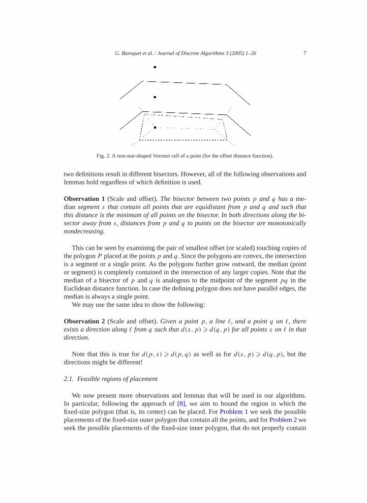
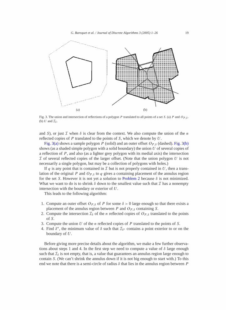
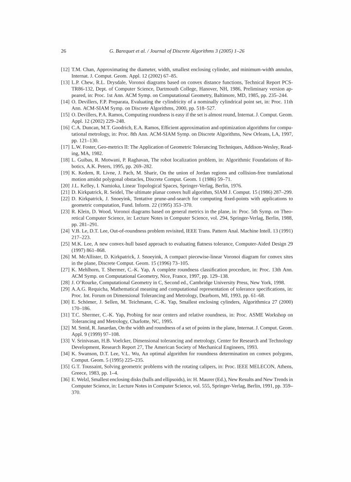
Fig. 3. The union and intersection of reflections of a polygonP translated to all points of a setS. (a)P andOP,δ .(b) U andIδ .

andS), or justI whenδ is clear from the context. We also compute the union of thn

reflected copies ofP translated to the points ofS, which we denote byU .Fig. 3(a)shows a sample polygonP (solid) and an outer offsetOP,δ (dashed).Fig. 3(b)

shows (as a shaded simple polygon with a solid boundary) the unionU of several copies oa reflection ofP , and also (as a lighter grey polygon with its medial axis) the intersecI of several reflected copies of the larger offset. (Note that the union polygonU is notnecessarily a single polygon, but may be a collection of polygons with holes.)

If q is any point that is contained inI but is not properly contained inU , then a translation of the originalP andOP,δ to q gives a containing placement of the annulus regfor the setS. However it is not yet a solution toProblem 2becauseδ is not minimized.What we want to do is to shrinkδ down to the smallest value such thatI has a nonemptyintersection with the boundary or exterior ofU .

This leads to the following algorithm:

1. Compute an outer offsetOP,δ of P for someδ > 0 large enough so that there existplacement of the annulus region betweenP andOP,δ containingS.

2. Compute the intersectionIδ of then reflected copies ofOP,δ translated to the pointof S.

3. Compute the unionU of then reflected copies ofP translated to the points ofS.4. Findδ∗, the minimum value ofδ such thatIδ∗ contains a point exterior to or on th

boundary ofU .

Before giving more precise details about the algorithm, we make a few further obstions about steps 1 and 4. In the first step we need to compute a value ofδ large enoughsuch thatIδ is not empty, that is, a value that guarantees an annulus region large enocontainS. (We can’t shrink the annulus down if it is not big enough to start with.) Toend we note that there is a semi-circle of radiusδ that lies in the annulus region betweenP


andOP,δ , and is centered inv, for every vertexv of P . Let w be the width of some axis-

ybeen

erly

with

e

tex of

ng the

e

at the

parallel bounding square that contains all ofS. Then, forδ = w√

5/2 there is a semi-circlecentered at the leftmost vertex ofP that lies in the annulus region betweenP andOP,δ

and which is large enough to contain the bounding square aroundS.7 Now we consider thefinal step. If we offsetIδ inward by some amount, sayα, the resulting polygon is simplIδ−α , the intersection polygon that would have resulted if the original outer offset hadδ − α instead ofδ. So in order to compute the minimal outer offsetδ∗, we really need onlycompute the value ofα that determines how far inward the polygonIδ can be offset.

This leads to a further observation. Equivalently to offsettingI inward until it no longercontains a point that is not properly contained inU , we could compute MA(I) and consideroffsettingI outward from its center until it contacts the first point that is not propcontained inU . (This approach is similar to that taken inSection 6.1.) Thus we have:

Lemma 20. Let the centerc of MA(I) be insideU . Consider an expanding offset ofIthat begins atc and grows outward. Then there is some pointx that is a first point on theboundary ofU hit by this expanding offset, andx is either a reflex vertex ofU or is on theintersection ofMA(I) and the boundary ofU .

Proof. We prove the claim by contradiction. Letx be a first point on the boundary ofU

that is hit by the expanding offset ofI. Suppose thatx is neither a reflex vertex ofU ,nor a point on MA(I). It follows thatx falls on some edgeei of the expandingI but noton a vertex ofI (since the vertices ofI move outward along MA(I)). Supposex is on avertex ofU . By our assumption, it is not a reflex vertex, and so it is a convex vertexrespect to the interior ofU . Thus at least one edge ofU adjacent tox is interior toI atthe moment the expandingei contactsx, but this would mean thatei intersected that edgbefore intersectingx, which is a contradiction of our assumption thatx is an initial contact.

Suppose instead, then, thatx is on an edgeeu of U , but is not a vertex ofU . If eu is notparallel toei , then one direction alongeu is closer to the inside ofI and thereforeei willintersecteu before it reachesx, which is a contradiction. However, ifei andeu are parallel,then the initial point of contact is a segment one of whose endpoints is either a verei (and thus on MA(I) which is a contradiction) or is a convex vertex ofeu, which weassumed was not the case.�

We now present a more detailed version of step 4 of the last algorithm, enhancidetails of the final step:

4. (a) Compute MA(I), and letc be its center.(b) Determine whetherc is properly contained inU . If it is not, then we are done. W

let α be the amount by which we offsetI inward until it degenerates to the pointc.Then ourδ − α is the width of the smallest annulus, andc is the translation of theannulus bounded byP andOP,δ−α that containsS.

7 √5/2 is the radius of a circle circumscribing a unit square, where the center of the circle is located

midpoint of one of the edges of the square.


(c) If c is properly contained inU , then we compute (usingLemma 20) the smallest

aref

cation

et

marize

case

flectedlces

ones

gy

n

e don’t

inner offsetα of I that contains a pointx not properly contained inU . Our optimalannulus region isδ − α and its containing translation is given byx.

7.2. Analysis

Step 1 requires O(n + m) time: O(n) time is required to compute a bounding squof S and O(m) time to offsetP by this much. In step 2 we compute the intersection on

copies of a convex polygon in O(n logn + m) time (or in O(n logh + m) time, whereh isthe size of the convex hull ofS).

In step 3 the union ofn copies of a convex polygon has complexity O(nm) and anexplicit version of it can be computed in O(nm(logn + logm)) time (Section 3.2). We cancompute MA(I) (in step 4) in O(m) time by using the technique of[2].

The last two parts of step 4 are the most complex. We can perform the point-loquery ofc in O(logn + logm) time. We then use ray-shooting for each of them edgesof MA(I) to determine where they intersectU . Conversely, we test each of then reflexvertices ofU to determine in which region of MA(I) it falls and then compute the offsat which the edge sweeps through it.

In the next section we provide one further enhancement of the algorithm and sumits running time.

7.3. Using a compact representation of the union

The running time of the algorithm can be reduced by almost a linear factor (in thewhenm andn are both large) by using a compact representation ofU : the union of thencopies of the reflection ofP . Note thatU has complexity O(nm), but only O(n) of thosevertices are reflex vertices representing the intersections of the boundaries of two recopies ofP , since the copies ofP form a family ofn pseudo-disks[19]. Furthermore, althe reflex vertices ofU are of these O(n) intersection-type vertices. The rest of the vertiare from some copy of the reflection ofP .

We want to compute a representation ofU that explicitly stores only these intersectivertices. As noted inSection 3.2, the portions ofU in between these intersection verticare just parts of chains of a copy of a reflection ofP and are stored implicitly with twopoints that specify what portion of a chain of which copy. This compact structureU∗ canbe computed in O(n logn(logn+ logm)+m) time by using a divide-and-conquer strate(Section 3.2). The reflex vertices needed in step 4(c) (seeLemma 20) are explicitly storedin U∗. It is only slightly more complex to compute the intersection of MA(I) with U . Weperform a O(logn)-time ray-shooting query onU∗ to determine which portion of a polygothe ray from MA(I) passes through, and then a second O(logm)-time ray-shooting queryon that particular portion of a polygon. (Note that these are not nested steps, since wneed to perform the second ray-shooting query until we know which region ofU∗ we aresearching.)

Thus, we have shown the following:


Theorem 21. Given a convexm-gonP and a setS of n points in the plane, we can deter-

withthere)

tvexlus isster.

solve

nulus

forn

ions to

ed inhullo findremalerous

itraryinter-

orted

mine the translation for the minimum outer offset ofP that contains all the points ofS inO(n logn(logn + logm) + m) time.

As in Section 6.1, this technique applies to scaled as well as offset annuli, butscaled polygons we replace the medial axis with the modified axis (as explainedbased on each edge moving at a different speed.

8. Conclusion and open problems

In this paper we give efficient algorithms forProblems 1 and 2, finding the smallesconstrained annulus containing a setS of n points, where the annulus is defined by a conm-gonP and the offset operation, and either the outer or inner boundary of the annufixed. These algorithms are simpler than previous approaches and asymptotically fa

We conclude by mentioning a few open problems:

Problem 5. Set a theoretical lower bound on the asymptotic running time required toProblem 2.

Problem 6. Give efficient solutions for the annulus placement problems when the anis defined by a simple polygon (not necessarily convex).

Problem 7. Give efficient solutions forProblem 2for polyhedra in 3-space.

Acknowledgements

The authors wish to thank Amy Briggs, Iuliana Marinov, and Jelena Ignjatovicwork on the implementations reported inAppendix A. Many thanks are also due to aanonymous referee for meticulously reading this manuscript and for many suggestimprove it.

Appendix A. Experimental results

As an experimental project, we implemented five of the six algorithms proposSection 3.1: Brute Force 1 (BF1), Brute Force 2 (BF2), Brute Force 1 with convex-preprocessing (BF1-CH), Brute Force 2 using convex hulls and rotating calipers textremal points (BF2-CH-RC), and Brute Force 2 using binary search to find extpoints (BF2-CH-BS). The algorithms were implemented in Java and tested on numtypes of polygons and point sets.

First, we implemented two procedures for computing the intersection of two arbconvex polygons (used in some of the methods). Our first procedure computes thesection by merging the list of halfplanes defining the convex polygons into a single s


ull ascode.

ter forich ise poly-

-BSt twocounts

ons. In

b

le-

(a) (b)

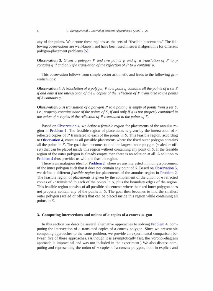
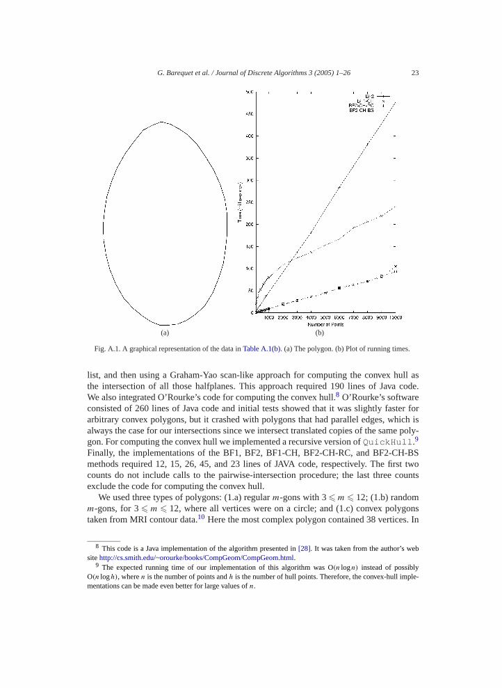
Fig. A.1. A graphical representation of the data inTable A.1(b). (a) The polygon. (b) Plot of running times.

list, and then using a Graham-Yao scan-like approach for computing the convex hthe intersection of all those halfplanes. This approach required 190 lines of JavaWe also integrated O’Rourke’s code for computing the convex hull.8 O’Rourke’s softwareconsisted of 260 lines of Java code and initial tests showed that it was slightly fasarbitrary convex polygons, but it crashed with polygons that had parallel edges, whalways the case for our intersections since we intersect translated copies of the samgon. For computing the convex hull we implemented a recursive version ofQuickHull.9

Finally, the implementations of the BF1, BF2, BF1-CH, BF2-CH-RC, and BF2-CHmethods required 12, 15, 26, 45, and 23 lines of JAVA code, respectively. The firscounts do not include calls to the pairwise-intersection procedure; the last threeexclude the code for computing the convex hull.

We used three types of polygons: (1.a) regularm-gons with 3� m � 12; (1.b) randomm-gons, for 3� m � 12, where all vertices were on a circle; and (1.c) convex polygtaken from MRI contour data.10 Here the most complex polygon contained 38 vertices

8 This code is a Java implementation of the algorithm presented in[28]. It was taken from the author’s wesitehttp://cs.smith.edu/~orourke/books/CompGeom/CompGeom.html.

9 The expected running time of our implementation of this algorithm was O(n logn) instead of possiblyO(n logh), wheren is the number of points andh is the number of hull points. Therefore, the convex-hull impmentations can be made even better for large values ofn.

http://cs.smith.edu/~orourke/books/CompGeom/CompGeom.html


00

15

,000

279021

00

05

3

,000

9519304

00

8770

,000

,377774153

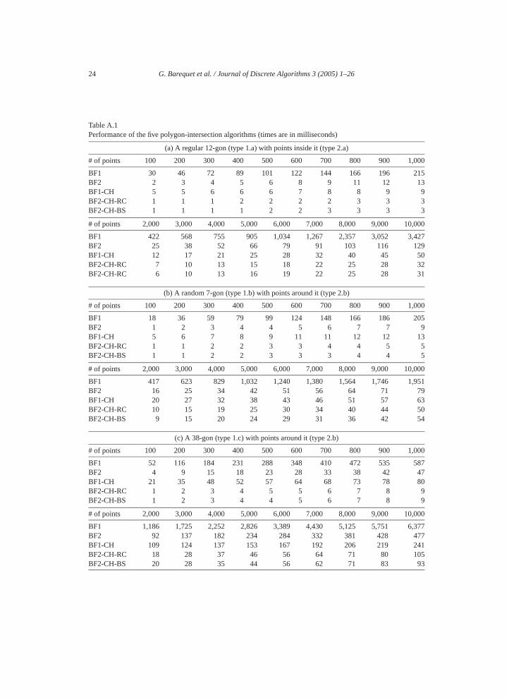
Table A.1Performance of the five polygon-intersection algorithms (times are in milliseconds)

(a) A regular 12-gon (type 1.a) with points inside it (type 2.a)

# of points 100 200 300 400 500 600 700 800 900 1,0

BF1 30 46 72 89 101 122 144 166 196 2BF2 2 3 4 5 6 8 9 11 12 13BF1-CH 5 5 6 6 6 7 8 8 9 9BF2-CH-RC 1 1 1 2 2 2 2 3 3 3BF2-CH-BS 1 1 1 1 2 2 3 3 3 3

# of points 2,000 3,000 4,000 5,000 6,000 7,000 8,000 9,000 10

BF1 422 568 755 905 1,034 1,267 2,357 3,052 3,4BF2 25 38 52 66 79 91 103 116 12BF1-CH 12 17 21 25 28 32 40 45 5BF2-CH-RC 7 10 13 15 18 22 25 28 3BF2-CH-RC 6 10 13 16 19 22 25 28 3

(b) A random 7-gon (type 1.b) with points around it (type 2.b)

# of points 100 200 300 400 500 600 700 800 900 1,0


# of points 2,000 3,000 4,000 5,000 6,000 7,000 8,000 9,000 10

BF1 417 623 829 1,032 1,240 1,380 1,564 1,746 1,BF2 16 25 34 42 51 56 64 71 7BF1-CH 20 27 32 38 43 46 51 57 6BF2-CH-RC 10 15 19 25 30 34 40 44 5BF2-CH-BS 9 15 20 24 29 31 36 42 5

(c) A 38-gon (type 1.c) with points around it (type 2.b)

# of points 100 200 300 400 500 600 700 800 900 1,0


# of points 2,000 3,000 4,000 5,000 6,000 7,000 8,000 9,000 10

BF1 1,186 1,725 2,252 2,826 3,389 4,430 5,125 5,751 6BF2 92 137 182 234 284 332 381 428 4BF1-CH 109 124 137 153 167 192 206 219 2BF2-CH-RC 18 28 37 46 56 64 71 80 10BF2-CH-BS 20 28 35 44 56 62 71 83 9


addition, we generated point sets (locations of the copies of the polygon) in two ways: (2.a)ed indn withon

er 100n the

cheds

tsttedethodwell as

rical

gram

ersal

: Proc.ience,ronoi’skraine,

lems,

, Dis-

points,

-width

s and

omput.

convex

points spread in the polygon interior with a uniform distribution; and (2.b) points locatanε-neighborhood of the boundary of a reflected copy of it.11 The points were first spaceequally along the polygon, then each point was offset independently from the polygoa uniform distribution in the range[−ε, ε]. Naturally, the number of copies of the polygwas identical to the number of points. In all our experiments the intersection of then copiesof a polygon was guaranteed to be nonempty. All the running times are averages ovtrials, each on a different random point set. All competing algorithms were tested osame sets of points. The size of the point sets ranged from 100 to 10,000.

The software was run on a 864 MHz Pentium III Dell computer with 256 KB camemory and 248 MB of RAM.Table A.1shows the results of running the five methoon three different polygons with numerous point sets. A plot of the data inTable A.1(c)isshown inFig. A.1. The size of the 38-gon was about 250× 250 units. For the experimenwith this polygon the value ofε was 10 units. The graph of the BF1 method was omibecause it was completely out of the scale of the other graphs. (That is, the BF1 mwas much slower than all the others.) As was demonstrated in these experiment (asin many others), the two leading methods were BF2-CH-RC and BF2-CH-BS.

References

[1] P.K. Agarwal, B. Aronov, M. Sharir, Exact and approximation algorithms for minimum-width cylindshells, Discrete Comput. Geom. 26 (2001) 307–320.

[2] A. Aggarwal, L.J. Guibas, J. Saxe, P.W. Shor, A linear-time algorithm for computing the Voronoi diaof a convex polygon, Discrete Comput. Geom. 4 (1989) 591–604.

[3] O. Aichholzer, D. Alberts, F. Aurenhammer, B. Gärtner, A novel type of skeleton for polygons, J. UnivComput. Sci. 1 (1995) 752–761 (an electronic journal).

[4] O. Aichholzer, F. Aurenhammer, Straight skeletons for general polygonal figures in the plane, in2nd Ann. Int. Computing and Combinatorics Conf., Hong Kong, in: Lecture Notes in Computer Scvol. 1090, Springer-Verlag, Berlin, 1996, pp. 117–126, Also appeared, in: P. Engel, H. Syta (Eds.), VoImpact on Modern Science, Book 2, Inst. of Mathematics of the National Academy of Sciences of UKiev, 1998, pp. 7–21.

[5] G. Barequet, A.J. Briggs, M.T. Dickerson, M.T. Goodrich, Offset-polygon annulus placement probComput. Geom. 11 (1998) 125–141.

[6] G. Barequet, M. Dickerson, M.T. Goodrich, Voronoi diagrams for polygon-offset distance functionscrete Comput. Geom. 25 (2001) 271–291.

[7] G. Barequet, M. Dickerson, P. Pau, Translating a convex polygon to contain a maximum number ofComput. Geom. 8 (1997) 167–179.

[8] M. de Berg, P. Bose, D. Bremner, S. Ramaswami, G. Wilfong, Computing constrained minimumannuli of point sets, Computer-Aided Design 30 (1998) 267–275.

[9] M. de Berg, M. van Kreveld, M. Overmars, O. Schwarzkopf, Computational Geometry: AlgorithmApplications, Springer-Verlag, Berlin, 1997.

[10] P. Bose, P. Morin, Testing the quality of manufactured balls and disks, Algorithmica, in press.[11] T.M. Chan, Optimal output-sensitive convex hull algorithms in two and three dimensions, Discrete C

Geom. 16 (1996) 361–368.

10 Available atftp://ftp.cs.technion.ac.il/pub/barequet/psdb.11 Here we don’t solve the annulus-matching problem, but only that of intersecting copies of the same

polygon.

ftp://ftp.cs.technion.ac.il/pub/barequet/psdb


[12] T.M. Chan, Approximating the diameter, width, smallest enclosing cylinder, and minimum-width annulus,

rt PCS-on ap-44.11th

. Geom.

mpu-997,

Read-

f Ro-

tional

299.ns to

Theo-, 1988,

1991)

sign 29

sites

h Ann.

98.ons, in:

2000)

hop on

t. Geom.

nology

gons,

thens,

nds inp. 359–

Internat. J. Comput. Geom. Appl. 12 (2002) 67–85.[13] L.P. Chew, R.L. Drysdale, Voronoi diagrams based on convex distance functions, Technical Repo

TR86-132, Dept. of Computer Science, Dartmouth College, Hanover, NH, 1986, Preliminary versipeared, in: Proc. 1st Ann. ACM Symp. on Computational Geometry, Baltimore, MD, 1985, pp. 235–2

[14] O. Devillers, F.P. Preparata, Evaluating the cylindricity of a nominally cylindrical point set, in: Proc.Ann. ACM-SIAM Symp. on Discrete Algorithms, 2000, pp. 518–527.

[15] O. Devillers, P.A. Ramos, Computing roundness is easy if the set is almost round, Internat. J. ComputAppl. 12 (2002) 229–248.

[16] C.A. Duncan, M.T. Goodrich, E.A. Ramos, Efficient approximation and optimization algorithms for cotational metrology, in: Proc. 8th Ann. ACM-SIAM Symp. on Discrete Algorithms, New Orleans, LA, 1pp. 121–130.

[17] L.W. Foster, Geo-metrics II: The Application of Geometric Tolerancing Techniques, Addison-Wesley,ing, MA, 1982.

[18] L. Guibas, R. Motwani, P. Raghavan, The robot localization problem, in: Algorithmic Foundations obotics, A.K. Peters, 1995, pp. 269–282.

[19] K. Kedem, R. Livne, J. Pach, M. Sharir, On the union of Jordan regions and collision-free translamotion amidst polygonal obstacles, Discrete Comput. Geom. 1 (1986) 59–71.

[20] J.L. Kelley, I. Namioka, Linear Topological Spaces, Springer-Verlag, Berlin, 1976.[21] D. Kirkpatrick, R. Seidel, The ultimate planar convex hull algorithm, SIAM J. Comput. 15 (1986) 287–[22] D. Kirkpatrick, J. Snoeyink, Tentative prune-and-search for computing fixed-points with applicatio

geometric computation, Fund. Inform. 22 (1995) 353–370.[23] R. Klein, D. Wood, Voronoi diagrams based on general metrics in the plane, in: Proc. 5th Symp. on

retical Computer Science, in: Lecture Notes in Computer Science, vol. 294, Springer-Verlag, Berlinpp. 281–291.

[24] V.B. Le, D.T. Lee, Out-of-roundness problem revisited, IEEE Trans. Pattern Anal. Machine Intell. 13 (217–223.

[25] M.K. Lee, A new convex-hull based approach to evaluating flatness tolerance, Computer-Aided De(1997) 861–868.

[26] M. McAllister, D. Kirkpatrick, J. Snoeyink, A compact piecewise-linear Voronoi diagram for convexin the plane, Discrete Comput. Geom. 15 (1996) 73–105.

[27] K. Mehlhorn, T. Shermer, C.-K. Yap, A complete roundness classification procedure, in: Proc. 13tACM Symp. on Computational Geometry, Nice, France, 1997, pp. 129–138.

[28] J. O’Rourke, Computational Geometry in C, Second ed., Cambridge University Press, New York, 19[29] A.A.G. Requicha, Mathematical meaning and computational representation of tolerance specificati

Proc. Int. Forum on Dimensional Tolerancing and Metrology, Dearborn, MI, 1993, pp. 61–68.[30] E. Schömer, J. Sellen, M. Teichmann, C.-K. Yap, Smallest enclosing cylinders, Algorithmica 27 (

170–186.[31] T.C. Shermer, C.-K. Yap, Probing for near centers and relative roundness, in: Proc. ASME Works

Tolerancing and Metrology, Charlotte, NC, 1995.[32] M. Smid, R. Janardan, On the width and roundness of a set of points in the plane, Internat. J. Compu

Appl. 9 (1999) 97–108.[33] V. Srinivasan, H.B. Voelcker, Dimensional tolerancing and metrology, Center for Research and Tech

Development, Research Report 27, The American Society of Mechanical Engineers, 1993.[34] K. Swanson, D.T. Lee, V.L. Wu, An optimal algorithm for roundness determination on convex poly

Comput. Geom. 5 (1995) 225–235.[35] G.T. Toussaint, Solving geometric problems with the rotating calipers, in: Proc. IEEE MELECON, A

Greece, 1983, pp. 1–4.[36] E. Welzl, Smallest enclosing disks (balls and ellipsoids), in: H. Maurer (Ed.), New Results and New Tre

Computer Science, in: Lecture Notes in Computer Science, vol. 555, Springer-Verlag, Berlin, 1991, p370.

Optimizing a constrained convex polygonal annulus

Documents

Transcript of Optimizing a constrained convex polygonal annulus