March 8, 2005 CBN 05-5

OPTIMIZED ANALYZING MAGNET FOR MEASUREMENTS OF POLARIZATION OF GAMMA QUANTS AT 10 MEV1

A. Mikhailichenko, Cornell University, LEPP, Ithaca NY 14853

Abstract. Described here are calculations and the test of the magnet for measurement of polarization of gammas by its helicity-dependent attenuation in magnetized iron. Magnet is a compact device which size is ~ten times smaller, than the worldwide analogues.

INTRODUCTION

Measurement of polarization of gammas in the energy range ~10MeV is a rather difficult task; however some procedures, including attenuation-dependence on polarization were developed and tested successfully. One of the mostly effective examples of usage of this method is probably [1], where helicity of neutrino was measured for the first time. Attenuation of 10 MeV-gammas is going mainly by two processes: electron-positron pair production and Compton scattering. Charged particles rapidly carry out energy of primary gamma beam. Electron-positron pair production occurs during interaction of gammas with nucleis of material, so it gives attenuation which does not depend on external magnetic field and pho ton polarization practically. Ratio of Compton cross section cσ to the cross section of pair creation pairσ (per atom) can be expressed

as αγσσ Zpairc /1/ ≅ [2], where γ stands for 2/ mcωγ h= , ce h/2=α , Z–is atomic number; for iron it is Z=26. For gammas with MeV10≅ωh , 20≅γ and the ratio goes to be

26.0/ ≅pairc σσ , i.e. pair creation dominates in attenuation. So the basics for measurements of polarization of gammas lies in spin dependence for cross-sections of Compton scattering only. By magnetizing the Iron target one can control spin orientation for electrons at outer shell. Electrons fill the orbits in Iron in the following way: 2, 8, 14 and 2. Unfortunately electrons at lower shells can not be polarized by external magnetic field. So we are talking about 2/26 of all electrons or ~7.7% of attenuation by Compton Effect (more exact number goes to 7.92%) and within this ~8% one needs to register spin dependent variation in attenuation of gammas passed through the magnetized target. Let see how it works. Total Compton cross section σ C can be written in the form [2]

+−

++−+

++=+= 20

22 )1(21

11

25

)1ln(2

12

22xx

xxxCpC

totC

σλξσσλξσσ (1)

whereσ π π0 02 2 2 2 25 22 5 10= = ≅ ⋅ −r e mc cm( / ) . , 2/2 mcx ωh= in the Lab frame, ( 4222 /4 cmx ωh=

in cm frame), λ = ±1 2/ is the electron helicity and ξ2 1= ± stands for helicity of the gamma beam. Unpolarized part can be described as the following [2]

1 Electronic version is available at http://www.lns.cornell.edu/public/CBN/2005/CBN05-5/cbn05-5.pdf. This work is supported by National Science Foundation.

2

+−+++

−−= 220

)1(218

21

)1ln(84

12

xxx

xxxCσ

σ

>>+

<<−=

1),(ln2

1),1(

21

20

203

8

xxxr

xxrππ

, (2)

and the polarization part in cross-section pσ can be seen from (1). Energy of the photon can be transferred to the electron in full with subtraction of the rest energy of electron, 2mcEe −= ωh . The ratio of a polarized component to an unpolarized one cp σσ / goes to be as represented in Fig. 1 below.

Figure 1: Ratio of polarized to unpolarized cross section, calculated with (1), (2) as function of x. In a case of our interest, MeV9≅ωh , 36≅x and ratio of these two components is~0.3. Summing up, the attenuation is going mostly by positron pair creation. Among full attenuation, ~21% is associated with Compton scattering. Within this 21%, ~7.9% of attenuation is associated with the polarization itself. Magnetic field dependence gives ~30% variation associated with spin, see Fig 1. So total variation in cross section associated in spin goes to be ~ 005.03.0079.021.0 ≅×× , i.e. ~0.5%. By flipping magnetic field direction this ratio can be raised to 1%. Meanwhile attenuation of flux is following the law

]2exp[)](exp[]exp[ 200 λξσσσσ pCpairtot nlnlFnlFF −×+×−×≅−×≅ , (3)

where l stands for the length of magnetized Iron target, n –is the number of Iron atoms per cm3. One can see from (3) that besides the absolute value of attenuation, asymmetry associated with magnetic field flip defined by spin dependent term only,

22 λξσδ pnlFFFF

≅+−

= −+

−+

, (4)

where signs + or – stand for sign of λ (in E-166 polarization of photons 2ξ is fixed and not flipped). So, this number depend on the target length, and in case of E-166, the asymmetry can reach 6% for Iron ~12 cm long [3].

3

Basically in E-166 there are two analyzing magnets with magnetized Iron: one for primary gamma-flux and the second one for gammas, re-converted from positrons, see Fig. 2. With this method polarization of positrons can be measured as well [3].

Figure 2: Equipment involved in measurement of positron polarization and gamma flux [3]. We represented here these formulas for better understanding the physical background of measurements with magnetized Iron. More detailed description of procedure one can find in E-166 project description [3].

SUGGESTED ANALYZING MAGNET FOR E-166

The basic idea here is that we wanted to make the coil as compact as possible with closest location to the core. This is due to the fact, that H

r defined by circulation around the feeding

current ∫ = NIldH π4.0rr

(H- in Gauss, dl-in cm, current I in Amperes, N stands for the number of

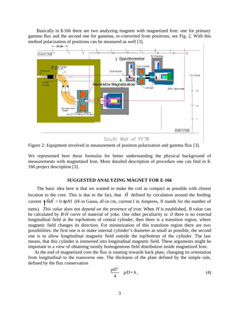
turns). This value does not depend on the presence of iron. When H is established, B value can be calculated by B-H curve of material of yoke. One other peculiarity is: if there is no external longitudinal field at the top/bottom of central cylinder, then there is a transition region, where magnetic field changes its direction. For minimization of this transition region there are two possibilities: the first one is to make internal cylinder’s diameter as small as possible, the second one is to allow longitudinal magnetic field outside the top/bottom of the cylinder. The last means, that this cylinder is immersed into longitudinal magnetic field. These arguments might be important in a view of obtaining mostly homogeneous field distribution inside magnetized Iron. At the end of magnetized core the flux is running towards back plate, changing its orientation from longitudinal to the transverse one. The thickness of the plate defined by the simple rule, defined by the flux conservation

hDD

×≅ ππ

4

2

, (4)

4

where D stands for diameter of the core, and h is the height of the plate. This yields 4/Dh ≅ i.e. half of radius. So the region of the core ~D/4 is lost for analyses. Situation can be improved if outside the core longitudinal Bx is present, so normal component is transferred from outside to inside region. This reguires configuration, when magnetized iron is sitting deep inside, so some fraction of the flux jumping out of iron (lowering in the plate in the Fig. 2 below must be deep).

Figure 2: Magnetized iron magnet.

Figure 3: Dimensions in millimeters.

5

All calculations carried out with MERMAID and results are represented below.

Figure 4: Field lines. ¼ of magnet is shown. The lines show equal-distant flux level.

Figure 5: Digital field map, kG

Figure 6: Enlarged digital map for the region around entrance.

6

Figure 7: Radial field as function of radial position. Numbers behind the filed B symbol mean the

radial distance in mm.

Figure 8: Longitudinal magnetic field values at different radiuses, left. Field amplitude B as

function of longitudinal distance for different radiuses, right. Field B at center as function of total current running in the coil is represented in Fig.9. One can see from there, that Iron is saturated at current ~4kA-turns and further growth is associated with raise of H field.

7

Figure 9: Maximal axes field, kG as a function of feeding current, kA-turns

So concluding, total current 10 kA-turns can be taken as maximal value for this magnet, although half of this value is enough for saturation.

ENGINEERING

Magnet yoke and core are made from annealed steel 1010. In this geometry, the total current, required for magnetization of core to ~23kG is ~10 kA. The coil made with n=12 × 4=48 turns, wound with single- length conductor having dimensions 4.76× 4.76 mm2 (3/16 × 3/16 in2) with a round hole for water flow measuring diameter 3.175 mm. Edges are rounded with radius 1mm (0.04 in). Total area of conductor’s cross-section is ~13.87 mm2. Average length of single turn is ~20 cm, yielding total conductor length ≅L 960 cm. Winding was done in two sets (so-called winding from the middle). First the main body of the coil was wound with exception of one-conductor thick radial layer. The volume occupied further with the coil was filled at this stage with a Teflon disc. Coil was impregnated by epoxy (Epotek T905). After this part of the coil was cured, the Teflon disc was removed and this radial spiral was filled with conductor kept in spare while winding first part of the coil. So after winding was finished, all ends were located at one external radial location. Resistance of conductor given in its specification is ft/408 Ωµρ ≅ or cm/38.13 Ωµ in metric units. So the total coil resistance goes to be

Ωρ 36 108.129601038.13 −− ⋅≅⋅×≅×= LR . (5)

As the saturated current taken is 10kA-turns, then the current running in conductor goes to be

8

An

II sat 208

4810000

1 ≅=≅ ,

and the power dissipated in all coils goes to be WRIP tot 5551028.1208 2221 ≅⋅×== − .

If we suggest, that water gains 10 degrees C passing through the coil, the flow rate in individual coil must be sec]/[012.0418610/][//][sec]/[ LWPcTWPLQ p ≅⋅== ∆ ≅ 12cm3/sec. The pressure drop P∆ in water channel, having length L can be defined from the following formula [4]

2/533 ][][

][104.6sec]/[ cmd

cmLatmP

cmQ∆

×≅ . (6)

This yields

psiatmd

LQatmP 1504.1

317.0101.496012

101.4][ 57

2

57

2

≅≅××

×≅

×××

≅∆

We expected that in reality the last number will be bigger, as the water hole becomes deformed while being wounded. The magnet fabricated is shown in Fig. 10.

Figure 10: Analyzing magnet.

9

TEST AND MEASUREMENTS

After fabrication the magnet was attached to the water line and powered up to 200 A. This current was limited by PC, however. PC voltage at 200 A goes to 9.4 V, so resistance is R=0.047O; this includes resistance associated with feeding cables. The water pressure at the input side was measured as 90 psi and at the out side it was 44 psi, so the pressure drop is somewhat 35 psi while water flow is 0.27gal/min. Remember, that calculations gave 15 psi pressure drop. So it is true, that conductor deformed its water hole. As one can see from (6), dependence on diameter is rather strong.

Figure 11: Measurements with Hall probe, installed on a movable cartridge.

Figure 12: Longitudinal field measured starting from the iron surface at the axis, see Fig. 11. Curves measured for 100 and 200A feeding current.

10

CONCLUSION

Usage of water-cooled conductor with moderate current density ~10A/mm2 allows compact design of analyzer with magnetized iron. That was proved by fabrication of such a magnet.

Figure 13: Our design, right, and the prototype, left, in comparison. The size of magnetized core is the same in these two magnets.

We made calculations of a prototype magnet, shown in Fig. 13, left and found that our magnet has the same properties concerning the magnetized core itself. Outer field in our magnet is a few times smaller, however. In conclusion Author thanks W.Trask for his help in assembling of this magnet.

REFERENCES

[1] M.Goldhaber, L.Grodzins, A.W.Sunyar,” Helicity of Neutrinos”, Phys.Rev.109:1015-1017, 1958. Available at http://prola.aps.org/pdf/PR/v109/i3/p1015_1.

[2] V.B. Berestetzky, E.M. Lifshits, L.P. Pitaevsky, “Quantum Electrodynamics”, Oxford, UK, Pergamon (1982) 652 p. (Course of Theoretical Physics, 4).

[3] SLAC-TN-04-018, “Undulator-Based Production of Polarized Positrons, A Proposal for the 50-GeV Beam in the FFTB”, (SLAC-PROPOSAL-E-166(bis)).

Available at http://www.slac.stanford.edu/pubs/slactns/slac-tn-04-018.html. [4] D.B. Montgomery, “Solenoid magnet design”, NY 1969.